EP3340203A1 - Traffic velocity estimation system - Google Patents
Traffic velocity estimation system Download PDFInfo
- Publication number
- EP3340203A1 EP3340203A1 EP16205483.7A EP16205483A EP3340203A1 EP 3340203 A1 EP3340203 A1 EP 3340203A1 EP 16205483 A EP16205483 A EP 16205483A EP 3340203 A1 EP3340203 A1 EP 3340203A1
- Authority
- EP
- European Patent Office
- Prior art keywords
- phase
- traffic
- velocity
- vehicle
- road network
- Prior art date
- Legal status (The legal status is an assumption and is not a legal conclusion. Google has not performed a legal analysis and makes no representation as to the accuracy of the status listed.)
- Granted
Links
Images



Classifications
-
- G—PHYSICS
- G08—SIGNALLING
- G08G—TRAFFIC CONTROL SYSTEMS
- G08G1/00—Traffic control systems for road vehicles
- G08G1/01—Detecting movement of traffic to be counted or controlled
- G08G1/0104—Measuring and analyzing of parameters relative to traffic conditions
- G08G1/0108—Measuring and analyzing of parameters relative to traffic conditions based on the source of data
- G08G1/0112—Measuring and analyzing of parameters relative to traffic conditions based on the source of data from the vehicle, e.g. floating car data [FCD]
-
- G—PHYSICS
- G08—SIGNALLING
- G08G—TRAFFIC CONTROL SYSTEMS
- G08G1/00—Traffic control systems for road vehicles
- G08G1/01—Detecting movement of traffic to be counted or controlled
- G08G1/0104—Measuring and analyzing of parameters relative to traffic conditions
- G08G1/0108—Measuring and analyzing of parameters relative to traffic conditions based on the source of data
- G08G1/0116—Measuring and analyzing of parameters relative to traffic conditions based on the source of data from roadside infrastructure, e.g. beacons
-
- G—PHYSICS
- G08—SIGNALLING
- G08G—TRAFFIC CONTROL SYSTEMS
- G08G1/00—Traffic control systems for road vehicles
- G08G1/01—Detecting movement of traffic to be counted or controlled
- G08G1/0104—Measuring and analyzing of parameters relative to traffic conditions
- G08G1/0108—Measuring and analyzing of parameters relative to traffic conditions based on the source of data
- G08G1/012—Measuring and analyzing of parameters relative to traffic conditions based on the source of data from other sources than vehicle or roadside beacons, e.g. mobile networks
-
- G—PHYSICS
- G08—SIGNALLING
- G08G—TRAFFIC CONTROL SYSTEMS
- G08G1/00—Traffic control systems for road vehicles
- G08G1/01—Detecting movement of traffic to be counted or controlled
- G08G1/0104—Measuring and analyzing of parameters relative to traffic conditions
- G08G1/0125—Traffic data processing
- G08G1/0129—Traffic data processing for creating historical data or processing based on historical data
-
- G—PHYSICS
- G08—SIGNALLING
- G08G—TRAFFIC CONTROL SYSTEMS
- G08G1/00—Traffic control systems for road vehicles
- G08G1/01—Detecting movement of traffic to be counted or controlled
- G08G1/0104—Measuring and analyzing of parameters relative to traffic conditions
- G08G1/0125—Traffic data processing
- G08G1/0133—Traffic data processing for classifying traffic situation
-
- G—PHYSICS
- G08—SIGNALLING
- G08G—TRAFFIC CONTROL SYSTEMS
- G08G1/00—Traffic control systems for road vehicles
- G08G1/01—Detecting movement of traffic to be counted or controlled
- G08G1/0104—Measuring and analyzing of parameters relative to traffic conditions
- G08G1/0137—Measuring and analyzing of parameters relative to traffic conditions for specific applications
- G08G1/0141—Measuring and analyzing of parameters relative to traffic conditions for specific applications for traffic information dissemination
-
- G—PHYSICS
- G08—SIGNALLING
- G08G—TRAFFIC CONTROL SYSTEMS
- G08G1/00—Traffic control systems for road vehicles
- G08G1/09—Arrangements for giving variable traffic instructions
- G08G1/0962—Arrangements for giving variable traffic instructions having an indicator mounted inside the vehicle, e.g. giving voice messages
- G08G1/0967—Systems involving transmission of highway information, e.g. weather, speed limits
- G08G1/096708—Systems involving transmission of highway information, e.g. weather, speed limits where the received information might be used to generate an automatic action on the vehicle control
- G08G1/096725—Systems involving transmission of highway information, e.g. weather, speed limits where the received information might be used to generate an automatic action on the vehicle control where the received information generates an automatic action on the vehicle control
-
- G—PHYSICS
- G08—SIGNALLING
- G08G—TRAFFIC CONTROL SYSTEMS
- G08G1/00—Traffic control systems for road vehicles
- G08G1/09—Arrangements for giving variable traffic instructions
- G08G1/0962—Arrangements for giving variable traffic instructions having an indicator mounted inside the vehicle, e.g. giving voice messages
- G08G1/0967—Systems involving transmission of highway information, e.g. weather, speed limits
- G08G1/096733—Systems involving transmission of highway information, e.g. weather, speed limits where a selection of the information might take place
- G08G1/096758—Systems involving transmission of highway information, e.g. weather, speed limits where a selection of the information might take place where no selection takes place on the transmitted or the received information
-
- G—PHYSICS
- G08—SIGNALLING
- G08G—TRAFFIC CONTROL SYSTEMS
- G08G1/00—Traffic control systems for road vehicles
- G08G1/09—Arrangements for giving variable traffic instructions
- G08G1/0962—Arrangements for giving variable traffic instructions having an indicator mounted inside the vehicle, e.g. giving voice messages
- G08G1/0967—Systems involving transmission of highway information, e.g. weather, speed limits
- G08G1/096766—Systems involving transmission of highway information, e.g. weather, speed limits where the system is characterised by the origin of the information transmission
- G08G1/096775—Systems involving transmission of highway information, e.g. weather, speed limits where the system is characterised by the origin of the information transmission where the origin of the information is a central station
Definitions
- the present invention relates to a system and method for accurate traffic velocity estimations.
- Modern navigation systems in vehicles include traffic flow estimation in order to provide users of vehicles with an estimated travel time for a particular route the user wants to take.
- traffic flow estimation is inaccurate and cumbersome since generally, only a limited number of sensors is available that provide sparse measurements of a real traffic situations in space and time.
- the main task in estimating the traffic flow is in processing these measurements and providing an estimate of a desired traffic variable for every position on a road and every point in time with the goal to reconstruct prevailing real traffic conditions most accurately.
- FCD Floating Car Data
- FCD Floating Car Data
- FCD Floating Car Data
- FCD Floating Car Data
- Another advantage of FCD is the ever-decreasing cost of retrieving said data such that FCD will be further increasingly available in the future.
- time intervals between two reported trajectories in a road segment of the road network can vary strongly.
- FCD usually do not explicitly contain traffic state data - e.g. data on a traffic density (traffic density data) and/or a traffic flow (traffic flow data).
- FCD is generally only sparsely available over the vehicle network. This sparsity of FCD and non-availability of traffic state data coupled with high spatiotemporal traffic dynamics along the road network are a major challenge for accurate traffic estimations.
- traffic flow estimation approaches have been introduced that take into consideration traffic dynamics.
- Said traffic flow estimation approaches can be classified into two categories.
- the first category comprises analytical flow models coupled with data assimilation techniques.
- traffic state data i.e. traffic flow data and traffic density data
- FCD traffic state data
- the second category of traffic flow estimation comprises estimation methods based on empirical traffic theory.
- one approach uses FCD for estimating velocities in the road network by classifying traffic on the road network into one of the following traffic phases: free-flow-phase, synchronized flow phase and wide moving jam phase.
- Other methods belonging to the second category of approaches apply basic filtering operations to measured data. They tend to unconditionally propagate low velocities up- and downstream although low velocities might be part of stationary congestion upstream a bottleneck. Hence, when only sparse probe data is available, the estimated velocities in stationary congestion patterns lack accuracy.
- a computer system for calculating accurate estimations of traffic velocity in a road network comprising:
- the at least one device may be e.g. an external device, e.g. a mobile device, which is assigned to a particular vehicle.
- the mobile device may be a smart phone that may run an appropriate application, app, providing the functionality to send the speed measurement data to the computational unit.
- the mobile device may send the speed measurement data to the computational unit e.g. whenever a connection allowing data transfer (e.g. Bluetooth, etc.) is established with the vehicle and the vehicle sends a notification to the device that it is in a driving mode.
- a connection allowing data transfer e.g. Bluetooth, etc.
- the computational unit may be a backend server. Alternatively or additionally, the computational unit may (at least partly) be located in a vehicle. Alternatively or additionally, the computational unit may be part of the road infrastructure corresponding to the road network.
- the at least one device may alternatively or additionally be a device integrated into the vehicle and providing the respective functionality for sending the speed measurement data, e.g. a navigation unit of the vehicle.
- the at least one device may be a traffic sensor located along a road in the road network operable to assess speed measurement data of vehicles passing the traffic sensor
- the at least one device may be integrated into a vehicle on the road providing speed measurement data of at least one other vehicle that is in the proximity of the vehicle the device is assigned to.
- the at least one device is a mobile device assessing speed measurement data of vehicles from above the road, e.g. a satellite, airplane, helicopter, quadrocopter.
- the speed measurement data may be sent when the vehicle is in a driving mode periodically, e.g. every 2 second (s), every 5 s, every 10s, every 20s, every 30s, or any other appropriate period of time for sending the speed measurement data.
- the speed measurement data may be floating car data, FCD.
- the speed measurement data may be sent each time a vehicle passes the traffic sensor.
- the external sensor measures the speed of a predetermined amount of vehicles passing the traffic sensor, calculate an average speed of the vehicles and send the calculated average speed as speed measurement data to the computational unit.
- FCD and speed measurement data will be used interchangeably hereinafter.
- Each region is defined as a part of a road segment of length L , wherein the size and the boundaries of said region may change over time. Over time, said region may further divide into two or more regions, or two or more regions may merge into one region.
- a road network may be a system of interconnecting lines and points (edges and nodes) that represent a system of streets or roads.
- the road network may be divided into one or more road segments. Further definitions for road network, road segment and region are provided below.
- each vehicle operating in an autonomous driving mode may use the data/information for determining a best route to a destination (e.g. if the velocity is rather low on one route, an alternative route with a better velocity may be autonomously chosen by the vehicle).
- the data/information on the velocity may be used in order to improve the security of all traffic participants in the road network, since the velocity data may be used by autonomous vehicles and/or by navigation systems of any vehicles to foresee road segments with low velocity and adapt the driving behavior accordingly.
- each speed measurement data comprises at least a location of a vehicle driving on the road network and a corresponding timestamp; and wherein each speed measurement data may further comprise:
- Each location of the vehicle may comprise a position of the vehicle at the road network.
- Each position may be obtained using navigation satellite systems comprising Global Positioning System (GPS), GLObal Navigation Satellite System (GLONASS), Galileo positioning system, and BeiDou Navigation Satellite System.
- GPS Global Positioning System
- GLONASS GLObal Navigation Satellite System
- Galileo positioning system Galileo positioning system
- BeiDou Navigation Satellite System BeiDou Navigation Satellite System.
- each position may be obtained from a respective module located in the vehicle.
- each GPS - position that may be determined by a GPS-Module located in the vehicle.
- each speed measurement data may comprise a current GPS-Position of the vehicle.
- the computational unit may track the position of the vehicle and determine position x along a corresponding road segment as part of the road network with x ⁇ [0, L ]. Each timestamp may correspond to a particular point in time t the vehicle was at the respective position x along the road segment.
- the GPS-Module may be located in the external device and in the traffic sensor, respectively (cf. above).
- the velocity of the vehicle may be calculated from the speed measurement data, as is explained in more detail below, or may be obtained from a speed sensor as e.g. located in the vehicle and/or in the traffic sensor.
- the direction of the vehicle c may be calculated from the speed measurement data or determined from a direction sensor that may be located in the vehicle.
- the lane the vehicle is currently driving on may be determined from further sensors, e.g. one or more cameras located in and/or on the vehicle and/or at the traffic sensor.
- the data on vehicles and their velocities surrounding the vehicle may be determined from further sensors, e.g. cameras, RAdio Detection And Ranging (RADAR) sensors, Light Detection And Ranging (LIDAR) sensors, photo sensors, thermal imaging cameras located in and/or on the vehicle, and/or any further appropriate sensors for providing the appropriate data.
- sensors e.g. cameras, RAdio Detection And Ranging (RADAR) sensors, Light Detection And Ranging (LIDAR) sensors, photo sensors, thermal imaging cameras located in and/or on the vehicle, and/or any further appropriate sensors for providing the appropriate data.
- identifying the regions comprises:
- calculating criteria probabilities P p i comprises the following: let P p 1 , P p 2 , ... , P p N k , P p i ⁇ R be N k p ⁇ N ⁇ 0 criteria that ( t , x ) needs to fulfill in order to belong to phase p, wherein each criterion is modelled as a fuzzy decider P p i ⁇ 0 1 .
- calculating accurate estimations of traffic velocity based on a prevailing traffic phase in the road network comprises:
- At least one of the vehicles driving on the road network supports an autonomous driving mode; wherein the computational unit is further operable to send the accurate estimations of traffic velocity to the vehicle supporting an autonomous driving mode; and wherein the vehicle supporting the autonomous driving mode is operable to take the accurate estimations of traffic velocity into account when operating in the autonomous driving mode.
- Vehicles comprising/supporting an autonomous driving mode for (at least in part) autonomously transporting passengers form one location to another are known.
- the autonomous driving mode is not yet available in a fully automated manner. Some vehicles require periodic input from an operator, e.g. a driver or passenger, whereas other vehicles and/or the driver of the vehicle may switch from a manual to an autonomous mode and vice versa, whenever applicable and/or allowable.
- the computational unit may send the accurate estimations of traffic velocity to all vehicles supporting an autonomous driving mode and previously registered via an appropriate application to the computational unit. Hence, the vehicles may use the accurate estimations of traffic velocity to the vehicles which may be taken into account of the respective vehicles for the autonomous driving mode.
- the computational unit may send the accurate estimations of traffic velocity to each vehicle previously registered at the computational unit, irrespective of whether the vehicle supports an autonomous driving mode.
- a navigation module of the vehicle may take the accurate estimations of traffic velocity into account for planning trips, warning drivers from jams and accurately predicting a time of arrival.
- a computer-implemented method for calculating accurate estimations of traffic velocity in a road network comprising:
- a computer program product comprising instructions thereon, which, when loaded and executed by at least one processor, cause the at least one processor to perform a method according to claim 13.
- a road network may be a system of interconnecting lines and points (edges and nodes) that represent a system of streets or roads.
- the road network may be divided into one or more road segments.
- each line (edge) between two interconnecting points (nodes) may be a road segment.
- the road network may be divided into road segments in any other appropriate manner.
- traffic on each road segment may be divided into three traffic phases.
- the first traffic phase is the free flow phase (in the following also referred to as: free flow).
- the free flow describes a state of traffic where traffic flow and traffic density are nearly in a linear relation. In the free flow, traffic demand is lower than a capacity of the respective road segment.
- the average velocity in free flow can be estimated to greater than or equal ( ⁇ ) 65 km/h (kilometers per hour) for roads with a speed limit greater of equal 85km/h or roads with unlimited speed limit.
- the second traffic phase is the synchronized flow phase (also referred to hereinafter as: synchronized) is characterized by high vehicle densities.
- the traffic demand corresponds to the capacity of the respective road segment.
- the average velocity of vehicles in synchronized flow is significantly lower than the average velocity of vehicles in free flow and can be estimated between 30km/h and 65 km/h.
- the variance of velocities among vehicles on different lanes of the road segment is lower than the variance of velocities in free flow traffic.
- a transition from free flow to synchronized flow can appear spontaneously on each road segment, e.g. due to local perturbations such as lane changing maneuvers and/or can be induced by moving jams propagating upstream.
- a transition from free flow to synchronized flow may infer a drop in the road capacity, e.g. at a bottleneck (e.g. an on/off-ramp), a closure of a lane and/or a beginning of a constructions site.
- a bottleneck e.g. an on/off-ramp
- the synchronized traffic phase may persist.
- the third traffic phase is the Wide Moving Jam (WMJ) - phase (in the following also referred to as WMJ).
- WMJ Wide Moving Jam
- the average velocity (hereinafter also referred to as mean velocity) in the WMJ can be estimated to lower than or equal ( ⁇ ) 30 km/h.
- the WMJ may occur spontaneously, e.g. when a vehicle in a synchronized decelerates stronger than necessary, resulting in a shockwave that propagates upstream (i.e. backwards from the decelerating vehicle) forming an upstream front of a WMJ.
- synchronized flow i.e. when vehicle density is high, it is likely that an over-deceleration happens. In this case, the average velocity can decrease down to 0 km/h.
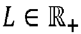
- a trajectory of a vehicle c ⁇ ⁇ 1, ...,N c ⁇ with N c a total number of vehicles (each vehicle corresponding to floating car data received at the computational unit), is a function x c ( t ) ⁇ [0, L ] denoting a position of vehicle c along a road segment with length L ⁇ R + at time t.
- Each road segment is a predefined part of the road network starting with a length unit (e.g. in m, km or any other appropriate unit of length) count of 0 and ending with length L ⁇ R + .
- An exemplary road segment is shown in Figure 4 , cf. 420.
- the derivative of the function x c ( t ) with respect to the time, v c (t), is the velocity of vehicle c at time (point in time) t.
- Each vehicle c passes a space-time domain [0, L ] ⁇ [0, T ] of a road segment with length L , observed for time period T , provides information about a part of the space-time domain.
- x 0 is the sum of a length of vehicle c (e.g. in centimeter cm, meter m, or any other appropriate unit of length representing the length of c) and a minimal distance to the preceding vehicle in queueing traffic.
- the minimal distance to the preceding vehicle in queueing traffic may be a constant, e.g. 1 m, 1.5m, 2m, 2.5m, 3m, 3.5 m or any other constant representing an appropriate or mandatory minimal distance to the preceding vehicle in queuing traffic.
- a "minimal space gap” is a non-constant space gap between a first vehicle to a preceding second vehicle that increases linearly with velocity v c ( t ) depending on time headway T 0 , wherein time headway T 0 is an elapsed time between a first point in time the preceding second vehicle finishes passing a fixed point at the road segment and the first vehicle starts to pass that fixed point at the road segment.
- PSM Phase-based Smoothing Method
- Figure 1 A shows an area ⁇ ( t, x ) (also referred to as area or area ⁇ ) represented by space interval [ x c ( t ), x c ( t ) + x 0 + T 0 ⁇ v c ( t )] at time t that vehicle c occupies.
- the occupied area ⁇ represented by space interval [ x c ( t ) , x c ( t ) + x 0 + T 0 ⁇ v c ( t )] in space-time (t, x) signifies that in this area ⁇ , only one vehicle c can exist on a single-laned road. Further, it is assumed that the vehicle's velocity is a representation of the traffic velocity in the occupied area.
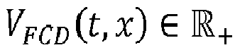
- V FCD t x ⁇ R + denotes the velocity data v c ( t ) reported by all (devices located in the corresponding) vehicles c combined into a single, two-dimensional function. This velocity is only valid in space-time ( t, x ) which is occupied by any vehicle c * (i.e.
- ⁇ t x ⁇ R denotes a kernel function and w t x ⁇ R a space-time-dependent weight of the input data, in this case the velocity measurements V FCD . Definitions of kernel functions and weightings are given further below.
- results of ⁇ V FCD need to be normalized.
- the normalization term is similar to the aforementioned convolution but omits velocity input V FCD :
- D w ⁇ t x ⁇ 0 T ⁇ 0 L ⁇ t ⁇ t ⁇ , x ⁇ x ⁇ ⁇ w t ⁇ x ⁇ ⁇ ⁇ t ⁇ x ⁇ d x ⁇ d t ⁇
- eq. (5) describes a common smoothing process, as depicted in Figure 1B . Then, for space-time ( t, x ) a weighted average velocity of all nearby velocities is computed (that are inside the occupied area ⁇ ( t , x )), where the weights depend on their distance to ( t, x ).
- FIG 2 shows the steps 200 performed for estimating accurate velocities V E 230 in the road network. These steps are performed using floating car data, FCD, but, however, may also be performed using any kind of speed measurement data. In particular, it is shown how the FCD (hereinafter also referred to as 'raw trajectory data') V FCD 210 is estimated into a continuous velocity estimate V E ( t, x ).
- FCD floating car data
- ⁇ ⁇ F,S,J ⁇ be the set of the phases 'Free Flow' (F), 'Synchronized Flow' (S) and 'Wide Moving Jam'; also referred to as 'WMJ' (J) (as outlined above).
- P p ( t, x ) ⁇ [0,1] with p ⁇ ⁇ denotes the probability for the traffic at time t and at position x to be in phase p.
- the FCD (also referred to herein as raw trajectory data) 210 is convolved with different smoothing kernels (cf. above, and equation (13)), resulting in smoothing data. Resulting values are evaluated to what extent they fulfill several fuzzy phase criteria. Respective criteria probabilities P p i t x denote the degree of fulfillment 221 at space-time (t, x).
- each traffic phase has different empirical characteristics, such as the aforementioned velocity ranges and respective traffic densities and traffic flows.
- the free flow phase has low traffic densities and high velocities, the synchronized flow phase lower velocities and higher densities and the Wide Moving Jam phase highest traffic densities and lowest velocity ranges.
- preliminary phase probability P p ′ is always lower or equal to the lowest criteria probability P p i .
- P p i the lowest criteria probability
- probability P U ⁇ [0,1] is estimated 223, which describes the level of uncertainty in assigning ( t, x ) to any of the phases.
- P U describes the probability that ( t, x ) does not belong to any of the phases:
- P U t x ⁇ p ⁇ ⁇ 1 ⁇ P p ′ t x
- a best-guess velocity V U For space-time (t, x) where the uncertainty is high a best-guess velocity V U needs to be assumed.
- the speed limit may be the best-guess velocity V U .
- other kinds of velocities e.g. historical averages, may be the best guess velocity V U .
- the dominance of the J-phase (WMJ-phase) is taken into account 224. Since P p ′ are independent, regions may occur especially in the presence of shockwaves, where both P J ′ and P S ′ or P F ′ estimate high probabilities. That is due to the different shapes of the convolution kernels and according velocities that are considered for the determination of the phase. Since WMJs can propagate through other phases without interruption (cf. equation (14)), plus, probability P J ′ is supported by more distinctive criteria, it is reasonable to assume that these regions rather belong to the J phase than to one of the others. Consequently, in those cases dominance of the J phase over the other phases is determined.
- P J t x P J ′ t x
- P S t x P S ′ t x ⁇ 1 ⁇ P J t x
- P F t x P F ′ t x ⁇ 1 ⁇ P J t x
- a velocity estimate V p H t x is computed 231.
- a fallback velocity V U ( t, x ) is assumed that serves as a best-guess velocity in case the uncertainty P U is high.
- the fallback velocity (also referred to herein as best-guess velocity) may be a speed limit. In another example, the fallback velocity may be a historical average velocity or any other appropriate velocity.
- V E ( t, x ) is determined 232 by aggregating the probabilities P p ( t, x ) and P U ( t, x ) and their respective velocity estimates V p H t x and V U ( t, x ).
- the first criterion is a velocity criterion P p 1 that uses velocity data of smoothed data for determining the phase probability.
- the second is a density criterion P p 2 .
- the density criterion P p 2 is applied to ensure that a phase hypothesis is supported by nearby data.
- density refers to the data or, in other word, the number of velocity measurements nearby.
- the velocity of vehicle c at time t v c ( t ) (herein also referred to as: 'velocity data') represents very important data for accurately determining to which traffic phase space-time (t, x) probably belongs to.
- the underlying idea of this criterion is to use velocity data measured in phase-characteristic directions around (t, x) and determine probability P p 1 .
- traffic breakdown is a probabilistic event triggered by perturbations.
- a traffic breakdown is usually connected to a capacity drop of the road infrastructure and a significant drop in average velocities. Consequently, velocity suits well to distinguish between free flow and congested flow.
- fuzzy thresholds v F thres and v S thres are applied.
- a fuzzy decider function ⁇ ( v, v thres , ⁇ ) (sigmoid function, i.e. a bounded differentiable real function that is defined for all real input values and has a positive derivative at each point) is applied that translates a velocity v into a probability P p 1 ⁇ 0 1 .
- Figure 3 shows the results of the sigmoid functions parameterized for free flow 310, synchronized flow 320 and WMJ 330 with respect to different velocities.
- V F t x V V FCD w 0 ⁇ F t x
- V S t x V V FCD w 0 ⁇ S t x with ⁇ F and ⁇ S denoting phase specific smoothing kernels, with characteristic speeds of v p dir and parameters ⁇ p and ⁇ p .
- the velocity criterion for the J phase is more distinct.
- ( t, x ) can only be assigned to the J phase if, both, up- and downstream of ( t, x ) low velocities are observed. Doing so ensures that WMJs are not extrapolated far beyond measurements in order to reduce wrongly estimated congested regions.
- ⁇ J u only considers data upstream of ( t, x )
- ⁇ J d only considers data downstream of ( t, x ). In that way data are smoothed in different directions.
- the combination of the sigmoid functions of the velocities V J u and V J d ensures that WMJs are only reconstructed in between low velocity measurements.
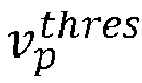
- eq. (13) uses different velocity thresholds v J thres and v S thres for the sigmoid functions. The difference stems from the expectation that once, due to downstream velocities below v J thres a WMJ is detected, this WMJ will propagate upstream as long as traffic upstream is in a state of critical flow-density (14). Since no density or flow data are available that state is assumed to be the congested region with the velocity threshold v S thres .
- the second criterion is a density criterion P p 2 t x that uses data density D (cf. equation (4) above) in order to quantify how well a phase hypothesis is supported by nearby data.
- This criterion enables coping with varying data density that comes along with FCD.
- P p 2 t x min 1 , D w 0 ⁇ p t x
- P p 2 equals to one if data is nearby, and converges to zero the greater the distance between ( t, x ) and the measurements.
- the validity of a measurement in space and time can be parametrized by adapting the kernel function or by modifying the weighting w 0 .
- phase probabilities P p ' is the product of all phase criteria P p 1 and P p 2 .
- a best-guess velocity V U ( t, x ) needs to be assumed.
- the speed limit is chosen in this example as best guess.
- other kinds of velocities can be chosen as best guess, e.g. historical velocity averages.
- the best-guess velocity V U ( t, x ) is used as fallback-velocity that serves as best-guess velocity in case the uncertainty is high.
- the raw trajectory data 210 was taken in order to calculate the appropriate traffic phases p in space and time using characteristic smoothing kernels and several criteria that allow distinguishing between them.
- the traffic phases p are taken to accurately calculating the traffic velocities.
- the traffic phases enable determining a region in space and time a velocity measurement has validity. For example, a low velocity measurement that is part of a Wide Moving Jam allows estimating the mean velocity of all vehicles that are part of the Wide Moving Jam. However, it does not enable a determination about a traffic velocity in an adjacent free flow or synchronized flow phase.
- V p H t x 1 V V FCD ⁇ 1 P p ⁇ p H t x
- V V FCD ⁇ 1 P p ⁇ p H t x denotes the convolution process (cf. equation (5)) smoothing the inverted trajectory velocities V V FCD ⁇ 1 with the convolution kernel ⁇ p H .
- V V FCD ⁇ 1 P p ⁇ p H t x denotes the convolution process (cf. equation (5)) smoothing the inverted trajectory velocities V V FCD ⁇ 1 with the convolution kernel ⁇ p H .
- a minimal velocity of 3 km / h is assumed. This enables that the smoothing process resembles a harmonic mean instead of an arithmetic one, which accounts for precision in travel time reconstruction (cf. equation (24)).
- the final phase probabilities P p are used as weights for the input data.
- each V p H mostly those measurements are taken into account that belong to phase p .
- convolution kernels ⁇ p H can be parametrized differently from the convolution kernels ⁇ p .
- the shapes of ⁇ p account for the characteristic propagation of phases, such as the propagation of J phases upstream and the stationary character of S phases.
- ⁇ p H on the other hand influence how data inside an already identified phase is smoothed, where data is weighted with respect to the final phase probabilities P p .
- a distinction between the parameters for example enables the reconstruction of a stationary synchronized flow phase with a large isotropic kernel ⁇ S and subsequently estimating velocities inside the phase with a smaller anisotropic kernel ⁇ S H that reconstructs minor shockwaves (narrow moving jams (14)) occurring inside the phase.
- Available sparse FCD consist of timestamps and GPS positions sampled anonymously by individual vehicles with sampling times between 20s and 30s.
- An installed filter in the processing unit of the equipped vehicles retains packages of data, wherein each package of data contains a plurality of FCD for covering the case that, the vehicle's velocity does not match an expected velocity.
- the expected velocity is a state machine that is influenced by individually recorded velocities and provided velocity estimates.
- the results are fractions of complete trajectories being reported, with the positive result that individuals cannot be tracked along their journey. That filter mechanism was introduced to ensure each driver's privacy. Still, in case of congestion, detailed velocity data was collected.
- Figure 4 shows raw trajectory data 210 for a road segment 420, 430 (i.e. the congestion on German highway A99 direction north) are displayed.
- the triangles 440 mark positions of on- and off-ramps along the road segment 420, 430.
- the pattern shows different characteristics often occurring in congested freeway traffic. As can be seen, around 7:45am, a moving jam phase emerged that evolved into a WMJ and induced a traffic breakdown at the on-ramp at position 10 km. The WMJ propagated further upstream and induced another traffic breakdown at a neighboring bottleneck. The pattern evolves into a General Pattern (GP) expanding over two bottlenecks where the downstream fronts of synchronized flow phases are fixed slightly downstream the on-ramp positions. In the pinch zone of the downstream synchronized flow phase a few WMJs originate and propagate upstream.
- GP General Pattern
- each tuple represents the mean velocity of the vehicle at space-time (t, x) referring to the center of the grid cell in space and time
- weight w E [0,1] is used to mark the part of the cell that is occupied by the vehicle. If two velocities of different trajectories are assigned to the same cell, their mean value is determined and the weights w are added.
- the discretization of the approach requires to discretize the continuous 2D convolution.
- An efficient implementation of the discrete 2D convolution can be performed e.g. using the Fast Fourier Transform.
- Figure 5 depicts the computation of the final phase probabilities P P (P J , P S and P F ) 510 computed with all available trajectories. Based on the final phase probabilities P P 510, for each phase p, a phase velocity V p H is computed 520. Finally, the velocity estimate V E 530 is shown. Next to V E 530, the probability (1 - P U ) 540 is depicted that can be interpreted as quality value, where a value of one means high and a value of zero means low certainty of the result.
- the first approach is the Generalized Adaptive Smoothing Method (GASM) that is based on the observation that shockwaves in congested traffic propagate upstream and shockwaves in free traffic propagate downstream.
- GASM Generalized Adaptive Smoothing Method
- the GASM is applied as described in " Treiber, M., and D. Helbing: An adaptive smoothing method for traffic state identification from incomplete information. Interface and Transport Dynamics, Vol. 32, 2003, pp. 343-360 " (Treiber) and van Lint, J. Empirical Evaluation of New Robust Travel Time Estimation Algorithms.
- FCD Transportation Research Record: Journal of the Transportation Research Board, 2160, 2010, pp. 50-59 " with an adaption to sparse FCD.
- the adaption describes how sparse FCD and a best-guess velocity can be fused in order to provide a continuous velocity estimate if no data is nearby.
- the weighting ratio of FC data to the velocity fallback is 1000:1.
- Parametrization is chosen according to Treiber. Further, an isotropic smoothing approach (na ⁇ ve approach) is applied that smooths data mostly in time and slightly in space.
- Applied PSM parameters are listed in Table 2.
- the velocity thresholds v p thres were explained above, the propagation directions v p dir have been set similar tomaschineer.
- the other parameters which are mainly the sizes of the kernels ⁇ p and ⁇ p H have been set with respect to typically observed properties of congestion: WMJs often have a higher spatial than temporal extent, thus ⁇ J is greater than ⁇ J .
- Synchronized flow phases are rather stationary or, if not, their downstream fronts usually stick to adjacent upstream bottlenecks and remain there.
- the kernel has a relatively high value ⁇ S compared to ⁇ S , which results in a larger temporal smoothing.
- Kernel ⁇ S H which is applied after identifying the S phase, is smaller in time but larger in space. Effectively, minor shockwaves are propagated correctly upstream.
- the kernels for the free flow phase are medium sized. In experiments, estimation accuracies were less sensitive to changes of these parameters.
- Table 2 Parameters for the presented approach (PSM) Parameter ⁇ Phase J S F ⁇ p 20s 300s 150s ⁇ p 500m 50m 100m v p dir -18 km/h 0 km/h 70 km/h v p thres 30 km/h 65 km/h 55 km/h ⁇ p 0.4 h/km 0.5 h/km 0.5 h/km ⁇ p H 20s 100s 150s ⁇ p H 500m 200m 100m v p dir , H -18 km/h -18 km/h 70 km/h
- Figure 6 shows the obtained estimation results applying the three approaches (PSM, GASM, na ⁇ ve) with limited data coverage, i.e. sparse FCD 610.
- the na ⁇ ve approach manages to estimate the stationary traffic upstream the two bottlenecks well but fails in reconstructing moving jams. It smooths the low velocities that actually propagate upstream in temporal direction only, such that the estimation of the congestion pattern s is inaccurate.
- the GASM-approach manages to reconstruct the moving jams more accurately than the na ⁇ ve approach, however, also here the estimation of velocities is wrong for many grid cells. For example, the latest moving jam is extrapolated further upstream than it actually propagated. Furthermore low velocities are smoothed slightly beyond the downstream bottleneck at kilometer 10. Further, the queueing traffic at the bottlenecks are not accurately estimated. Zones that are actually in congested state are estimated as free flow.
- the PSM-approach manages to accurately distinguish between the queueing traffic at the bottlenecks and the WMJs.
- the gaps in data that belong to moving jams are correctly classified as J phase and respective low velocities are estimated.
- Gaps in the stationary traffic upstream the bottlenecks are accurately reconstructed as synchronized flow phases such that appropriate velocities are estimated from data in the same phase.
- An expected estimation failure occurs at 8:00am where the moving synchronized flow is treated as stationary congestion and velocities are smoothed in temporal direction. That improves as the velocities drop further and a J phase is identified.
- estimated phase fronts by the PSM have sharper edges. This improved accuracy is very valuable feature for using the fronts for predictions in a navigation system and/or hazard warnings, especially for autonomous driving.
- the set of N c trajectories is divided into a training set and a test set.
- the training set is used in order to estimate velocities V E , and the test set is used to evaluate the accuracy of that estimate.
- N E ⁇ 1 ⁇ ⁇ N c
- ⁇ E denominates the number of trajectories per hour that are used for the estimation process.
- MAPE Mean Absolute Percentage Error
- Figure 7 shows the MAPE with respect to data densities ⁇ E between 10 traces/hour and 90 traces/hour for the na ⁇ ve approach 710, the GASM approach 720 and the PSM approach 730.
- the presented error values are the mean MAPE of 50 iterations with randomly assigned training and test set in order to ensure robustness of the results.
Landscapes
- Physics & Mathematics (AREA)
- General Physics & Mathematics (AREA)
- Chemical & Material Sciences (AREA)
- Analytical Chemistry (AREA)
- Life Sciences & Earth Sciences (AREA)
- Atmospheric Sciences (AREA)
- Traffic Control Systems (AREA)
Abstract

Description
- The present invention relates to a system and method for accurate traffic velocity estimations.
- Modern navigation systems in vehicles include traffic flow estimation in order to provide users of vehicles with an estimated travel time for a particular route the user wants to take. However, traffic flow estimation is inaccurate and cumbersome since generally, only a limited number of sensors is available that provide sparse measurements of a real traffic situations in space and time. The main task in estimating the traffic flow is in processing these measurements and providing an estimate of a desired traffic variable for every position on a road and every point in time with the goal to reconstruct prevailing real traffic conditions most accurately.
- In recent years, the availability of Floating Car Data (FCD) or other speed measurement data corresponding to the speed of a traffic flow in the road network has quickly spread and is increasingly available for traffic flow estimation in a road network. Using FCD is advantageous since it provides the possibility to obtain traffic data on each position along a road network. Besides this highly spatial resolution of available data, another advantage of FCD is the ever-decreasing cost of retrieving said data such that FCD will be further increasingly available in the future. However, time intervals between two reported trajectories in a road segment of the road network can vary strongly. In addition, FCD usually do not explicitly contain traffic state data - e.g. data on a traffic density (traffic density data) and/or a traffic flow (traffic flow data). Further, FCD is generally only sparsely available over the vehicle network. This sparsity of FCD and non-availability of traffic state data coupled with high spatiotemporal traffic dynamics along the road network are a major challenge for accurate traffic estimations.
- To address the above problems, traffic flow estimation approaches have been introduced that take into consideration traffic dynamics. Said traffic flow estimation approaches can be classified into two categories. The first category comprises analytical flow models coupled with data assimilation techniques. However, in practice, said traffic flow estimation approaches require traffic state data (i.e. traffic flow data and traffic density data) in addition to FCD, thereby limiting the applicability in large scale since it adds further complexity to data acquisition and data processing for traffic flow estimation. The second category of traffic flow estimation comprises estimation methods based on empirical traffic theory. In particular, one approach uses FCD for estimating velocities in the road network by classifying traffic on the road network into one of the following traffic phases: free-flow-phase, synchronized flow phase and wide moving jam phase. A major drawback, however, is that velocities within the traffic phases are estimated as constant over space and time. Doing so strongly limits the accuracy of the said traffic phase estimations. Other methods belonging to the second category of approaches apply basic filtering operations to measured data. They tend to unconditionally propagate low velocities up- and downstream although low velocities might be part of stationary congestion upstream a bottleneck. Hence, when only sparse probe data is available, the estimated velocities in stationary congestion patterns lack accuracy.
- Therefore, it is an object of the present invention to overcome the above-mentioned drawbacks by accurately estimating traffic velocity along a road network based on sparse probe data as input.
- This problem is solved by the independent claims. Preferred embodiments are described in the dependent claims.
- According to a first aspect, a computer system for calculating accurate estimations of traffic velocity in a road network, the system comprising:
- a plurality of devices, each device operable to deliver speed measurement data corresponding to the speed of a traffic flow in the road network; and
- at least one computational unit,
- wherein each of the plurality of devices sends speed measurement data to the computational unit, and
- wherein the computational unit is operable to calculate accurate estimations of traffic velocity in the road network by:
- identifying regions with varying sizes and moving boundaries under the condition that within each region, a corresponding traffic phase p is constant, wherein each traffic phase is one of a free-flow phase, a synchronized phase or a wide moving jam phase;
and - calculating (230) accurate estimations of traffic velocity in said regions based on the corresponding traffic phases.
- identifying regions with varying sizes and moving boundaries under the condition that within each region, a corresponding traffic phase p is constant, wherein each traffic phase is one of a free-flow phase, a synchronized phase or a wide moving jam phase;
- The at least one device may be e.g. an external device, e.g. a mobile device, which is assigned to a particular vehicle. E.g. the mobile device may be a smart phone that may run an appropriate application, app, providing the functionality to send the speed measurement data to the computational unit. The mobile device may send the speed measurement data to the computational unit e.g. whenever a connection allowing data transfer (e.g. Bluetooth, etc.) is established with the vehicle and the vehicle sends a notification to the device that it is in a driving mode.
- The computational unit may be a backend server. Alternatively or additionally, the computational unit may (at least partly) be located in a vehicle. Alternatively or additionally, the computational unit may be part of the road infrastructure corresponding to the road network.
The at least one device may alternatively or additionally be a device integrated into the vehicle and providing the respective functionality for sending the speed measurement data, e.g. a navigation unit of the vehicle. - Alternatively or additionally, the at least one device may be a traffic sensor located along a road in the road network operable to assess speed measurement data of vehicles passing the traffic sensor
- Alternatively or additionally, the at least one device may be integrated into a vehicle on the road providing speed measurement data of at least one other vehicle that is in the proximity of the vehicle the device is assigned to.
- Alternatively or additionally, the at least one device is a mobile device assessing speed measurement data of vehicles from above the road, e.g. a satellite, airplane, helicopter, quadrocopter.
- The speed measurement data may be sent when the vehicle is in a driving mode periodically, e.g. every 2 second (s), every 5 s, every 10s, every 20s, every 30s, or any other appropriate period of time for sending the speed measurement data. In the example where the at least one device is or comprises an external device (cf. above) or is integrated into the vehicle, the speed measurement data may be floating car data, FCD. In the example where the at least one device is or comprises a traffic sensor, the speed measurement data may be sent each time a vehicle passes the traffic sensor. Alternatively, the external sensor measures the speed of a predetermined amount of vehicles passing the traffic sensor, calculate an average speed of the vehicles and send the calculated average speed as speed measurement data to the computational unit. The terms FCD and speed measurement data will be used interchangeably hereinafter.
- Each region is defined as a part of a road segment of length L, wherein the size and the boundaries of said region may change over time. Over time, said region may further divide into two or more regions, or two or more regions may merge into one region.
- A road network may be a system of interconnecting lines and points (edges and nodes) that represent a system of streets or roads. The road network may be divided into one or more road segments. Further definitions for road network, road segment and region are provided below.
- Especially in view of the vehicles supporting an autonomous driving mode, the accurate estimation of traffic velocity is no longer just a tool for estimating a travel time for a particular route to a driver, but rather represents important data for road safety in view of improving the autonomous driving mode. In particular, on the one hand, each vehicle operating in an autonomous driving mode may use the data/information for determining a best route to a destination (e.g. if the velocity is rather low on one route, an alternative route with a better velocity may be autonomously chosen by the vehicle). On the other hand, the data/information on the velocity may be used in order to improve the security of all traffic participants in the road network, since the velocity data may be used by autonomous vehicles and/or by navigation systems of any vehicles to foresee road segments with low velocity and adapt the driving behavior accordingly.
- According to an embodiment,
each speed measurement data comprises at least a location of a vehicle driving on the road network and a corresponding timestamp; and
wherein each speed measurement data may further comprise: - a velocity of the vehicle at a point in time corresponding to the timestamp;
- a direction of the vehicle at the point in time corresponding to the timestamp;
- a lane the vehicle is driving on; and/or
- Each location of the vehicle may comprise a position of the vehicle at the road network. Each position may be obtained using navigation satellite systems comprising Global Positioning System (GPS), GLObal Navigation Satellite System (GLONASS), Galileo positioning system, and BeiDou Navigation Satellite System. In particular, each position may be obtained from a respective module located in the vehicle. In the example of the Global Positioning System, each GPS - position that may be determined by a GPS-Module located in the vehicle. In this example, each speed measurement data may comprise a current GPS-Position of the vehicle. Since the vehicle (or the device corresponding to the vehicle) transmits speed measurement data comprising corresponding GPS-data to the computational unit, the computational unit may track the position of the vehicle and determine position x along a corresponding road segment as part of the road network with x ∈ [0, L]. Each timestamp may correspond to a particular point in time t the vehicle was at the respective position x along the road segment. The GPS-Module may be located in the external device and in the traffic sensor, respectively (cf. above).
- The velocity of the vehicle may be calculated from the speed measurement data, as is explained in more detail below, or may be obtained from a speed sensor as e.g. located in the vehicle and/or in the traffic sensor.
- The direction of the vehicle c may be calculated from the speed measurement data or determined from a direction sensor that may be located in the vehicle.
- The lane the vehicle is currently driving on may be determined from further sensors, e.g. one or more cameras located in and/or on the vehicle and/or at the traffic sensor.
- The data on vehicles and their velocities surrounding the vehicle (sending the speed measurement data) may be determined from further sensors, e.g. cameras, RAdio Detection And Ranging (RADAR) sensors, Light Detection And Ranging (LIDAR) sensors, photo sensors, thermal imaging cameras located in and/or on the vehicle, and/or any further appropriate sensors for providing the appropriate data.
- According to a further embodiment, identifying the regions comprises:
- calculating, from the speed measurement data, criteria probabilities

- calculating, as the product of all criteria probabilities, the independent probability

- estimating the uncertainty probability PU ∈ [0,1], wherein PU describes a level of uncertainty in assigning (t, x) to any of the phases p;
- taking into account the dominance of the wide moving jam phase; and
- determining final phase probabilities Pp ;
- According to a further embodiment, calculating criteria probabilities


- According to a further embodiment, the independent probability


- According to a further embodiment, the uncertainty probability PU ∈ [0,1] that describes the probability that (t, x) does not belong to any of the phases Ω is calculated by:

- According to a further embodiment, if there is an occurrence of a high probability of a region belonging to


- According to yet a further embodiment, determining the final phase probabilities Pp while taking into account the dominance of


- According to a further embodiment, calculating accurate estimations of traffic velocity based on a prevailing traffic phase in the road network comprises:
- estimating phase-dependent velocity estimates

- aggregating final-phase probabilities Pp and corresponding velocity estimates

- According to a further embodiment, estimating phase-dependent velocity estimates


- According to another embodiment, aggregating final-phase probabilities Pp and the corresponding velocity estimates


- According to yet another embodiment, at least one of the vehicles driving on the road network supports an autonomous driving mode;
wherein the computational unit is further operable to send the accurate estimations of traffic velocity to the vehicle supporting an autonomous driving mode; and
wherein the vehicle supporting the autonomous driving mode is operable to take the accurate estimations of traffic velocity into account when operating in the autonomous driving mode. - Vehicles comprising/supporting an autonomous driving mode for (at least in part) autonomously transporting passengers form one location to another are known. However, the autonomous driving mode is not yet available in a fully automated manner. Some vehicles require periodic input from an operator, e.g. a driver or passenger, whereas other vehicles and/or the driver of the vehicle may switch from a manual to an autonomous mode and vice versa, whenever applicable and/or allowable. In order to improve the security and efficiency of autonomous driving modes, the computational unit may send the accurate estimations of traffic velocity to all vehicles supporting an autonomous driving mode and previously registered via an appropriate application to the computational unit. Hence, the vehicles may use the accurate estimations of traffic velocity to the vehicles which may be taken into account of the respective vehicles for the autonomous driving mode. The security and efficiency of the autonomous driving mode is hence greatly improved. Alternatively and/or additionally, the computational unit may send the accurate estimations of traffic velocity to each vehicle previously registered at the computational unit, irrespective of whether the vehicle supports an autonomous driving mode. In this example, a navigation module of the vehicle may take the accurate estimations of traffic velocity into account for planning trips, warning drivers from jams and accurately predicting a time of arrival.
- According to another aspect, a computer-implemented method for calculating accurate estimations of traffic velocity in a road network is provided, the method comprising:
- sending, by a plurality of devices, speed measurement data to a computational unit, wherein each speed measurement data corresponds to the speed of a traffic flow in the road network,
- and
- calculating, by the computational unit, accurate estimations of traffic velocity in the road network by:
- identifying regions with varying sizes and moving boundaries under the condition that within each region, a corresponding traffic phase p is constant, wherein each traffic phase is one of a free-flow phase, a synchronized phase or a wide moving jam phase; and
- calculating accurate estimations of traffic velocity in said regions based on the corresponding traffic phase.
- According to another aspect, a computer program product is provided comprising instructions thereon, which, when loaded and executed by at least one processor, cause the at least one processor to perform a method according to claim 13.
- The aspects defined above and further aspects of the present invention are apparent from the examples of embodiment to be described hereinafter and are explained with reference to the examples of embodiment. The invention will be described in more detail hereinafter with reference to examples of embodiment. However, it is apparent to the person skilled in the art that the invention is not limited to the examples of embodiment.
- Figure 1A
- shows an areaΨ(t, x) represented by a space interval [xc (t), xc (t) + x 0 + T 0 · vc (t)] of one vehicle at time t;
- Figure 1B
- shows a smoothing operation on FCD;
- Figure 2
- shows steps performed for estimating accurate velocities in a road network;
- Figure 3
- shows results of the sigmoid functions parameterized for free flow, synchronized flow and WMJ;
- Figure 4
- shows raw trajectory data for a road segment;
- Figure 5
- shows a computation of the final phase probabilities PP, the phase-dependent velocity estimates

- Figure 6
- shows obtained estimation results applying three approaches PSM, GASM and naïve; and
- Figure 7
- shows the MAPE with respect to data densities between 10 traces/hour and 90 traces/hour for the naïve approach, the GASM approach and the PSM approach.
- A road network may be a system of interconnecting lines and points (edges and nodes) that represent a system of streets or roads. The road network may be divided into one or more road segments. For example, each line (edge) between two interconnecting points (nodes) may be a road segment. However, the road network may be divided into road segments in any other appropriate manner. Moreover, traffic on each road segment may be divided into three traffic phases. The first traffic phase is the free flow phase (in the following also referred to as: free flow). The free flow describes a state of traffic where traffic flow and traffic density are nearly in a linear relation. In the free flow, traffic demand is lower than a capacity of the respective road segment. Therefore, there may exist a high spread of velocities between vehicles driving on different lanes of the road segment. The average velocity in free flow can be estimated to greater than or equal (≥) 65 km/h (kilometers per hour) for roads with a speed limit greater of equal 85km/h or roads with unlimited speed limit.
- The second traffic phase is the synchronized flow phase (also referred to hereinafter as: synchronized) is characterized by high vehicle densities. In particular, the traffic demand corresponds to the capacity of the respective road segment. The average velocity of vehicles in synchronized flow is significantly lower than the average velocity of vehicles in free flow and can be estimated between 30km/h and 65 km/h. Further, the variance of velocities among vehicles on different lanes of the road segment is lower than the variance of velocities in free flow traffic. A transition from free flow to synchronized flow can appear spontaneously on each road segment, e.g. due to local perturbations such as lane changing maneuvers and/or can be induced by moving jams propagating upstream. A transition from free flow to synchronized flow may infer a drop in the road capacity, e.g. at a bottleneck (e.g. an on/off-ramp), a closure of a lane and/or a beginning of a constructions site. When a maximum road capacity reduces and the traffic demand does to significantly change, the synchronized traffic phase may persist.
- The third traffic phase is the Wide Moving Jam (WMJ) - phase (in the following also referred to as WMJ). The average velocity (hereinafter also referred to as mean velocity) in the WMJ can be estimated to lower than or equal (≤) 30 km/h. The WMJ may occur spontaneously, e.g. when a vehicle in a synchronized decelerates stronger than necessary, resulting in a shockwave that propagates upstream (i.e. backwards from the decelerating vehicle) forming an upstream front of a WMJ. In synchronized flow, i.e. when vehicle density is high, it is likely that an over-deceleration happens. In this case, the average velocity can decrease down to 0 km/h.
- A trajectory of a vehicle c ∈ {1, ...,N c } with Nc = a total number of vehicles (each vehicle corresponding to floating car data received at the computational unit), is a function xc (t) ∈ [0, L] denoting a position of vehicle c along a road segment with length
- Each road segment is a predefined part of the road network starting with a length unit (e.g. in m, km or any other appropriate unit of length) count of 0 and ending with length

Figure 4 , cf. 420. - Accordingly, the derivative of the function xc (t) with respect to the time, vc(t), is the velocity of vehicle c at time (point in time) t.
- Each vehicle c passes a space-time domain [0, L] × [0, T] of a road segment with length L, observed for time period T, provides information about a part of the space-time domain.
- x 0 is the sum of a length of vehicle c (e.g. in centimeter cm, meter m, or any other appropriate unit of length representing the length of c) and a minimal distance to the preceding vehicle in queueing traffic. The minimal distance to the preceding vehicle in queueing traffic may be a constant, e.g. 1 m, 1.5m, 2m, 2.5m, 3m, 3.5 m or any other constant representing an appropriate or mandatory minimal distance to the preceding vehicle in queuing traffic.
- A "minimal space gap" is a non-constant space gap between a first vehicle to a preceding second vehicle that increases linearly with velocity vc (t) depending on time headway T
0 , wherein time headway T 0 is an elapsed time between a first point in time the preceding second vehicle finishes passing a fixed point at the road segment and the first vehicle starts to pass that fixed point at the road segment. - The present approach presented within this application is also referred to as novel Phase-based Smoothing Method (PSM) approach.
- In view of the above definitions,
Figure 1 A shows an area Ψ(t, x) (also referred to as area or area Ψ) represented by space interval [xc (t), xc (t) + x 0 + T 0·vc (t)] at time t that vehicle c occupies. The occupied area Ψ represented by space interval [xc (t), xc (t) + x 0 + T 0 ·vc (t)] in space-time (t, x) signifies that in this area Ψ, only one vehicle c can exist on a single-laned road. Further, it is assumed that the vehicle's velocity is a representation of the traffic velocity in the occupied area. - In other words, area Ψ(t, x) is a function that indicates whether at
time t 120, position x 110 (wherein x 110 is an arbitrary position along the road segment with x ∈ [0, L]) is occupied by any observed vehicle c:
time t 120, position x 110 is occupied) and 0 = false (i.e. attime t 120, position x 110 is not occupied), wherein
Ψ (t, x) has the following properties: - (a) if traffic density is high, all vehicles c keep a time headway of T 0 to their preceding vehicles and all vehicle positions x ∈ [0, L] at the road segment as well as velocities are known, then Ψ(t, x) = 1, ∀t ∈ [0, T], x ∈ [0, L].
- (b) if traffic density is low and gaps between vehicles are high, there are times and positions where Ψ(t, x) = 0;
- (c) if only for a part of all existent vehicles c their trajectories and velocities are known, then occupied part decreases the smaller the penetration rate of observed vehicles c.
- Accordingly,

- In order to process data locally, the two-dimensional convolution is a common and often used operation. The function


FCD need to be normalized. The normalization term is similar to the aforementioned convolution but omits velocity input VFCD :
- Later, applied kernel Φ(t, x) and weighting w(t, x) are chosen in such away that D(w,Φ,t,x) represents an estimate of the data density in the regions. The normalized convolution of weighted and velocity function Vc (t, x) with kernel Φ(t, x) is then stated as:

- For example, given a kernel function that returns only positive/zero values and has its maximum at (0,0), eq. (5) describes a common smoothing process, as depicted in
Figure 1B . Then, for space-time (t, x) a weighted average velocity of all nearby velocities is computed (that are inside the occupied area Ψ(t, x)), where the weights depend on their distance to (t, x). - The convolution kernel Φ allows a great variety of operations in general. Within the scope of the present subject-matter, the convolution kernel Φ is used for smoothing operations. For traffic related smoothing with characteristic wave speeds, the following simple and effective kernel formulation is also adopted here:

Figure 1B , a kernel with negative velocity vdir is depicted exemplarily as a discrete contourplot. Note that Φ is actually a continuous function. -
Figure 2 shows thesteps 200 performed for estimating accurate velocities VE 230 in the road network. These steps are performed using floating car data, FCD, but, however, may also be performed using any kind of speed measurement data. In particular, it is shown how the FCD (hereinafter also referred to as 'raw trajectory data')V FCD 210 is estimated into a continuous velocity estimate VE (t, x). - First, a calculation of final phase probabilities PP is performed 220.
- Let Ω = {F,S,J} be the set of the phases 'Free Flow' (F), 'Synchronized Flow' (S) and 'Wide Moving Jam'; also referred to as 'WMJ' (J) (as outlined above). Then, Pp (t, x) ∈ [0,1] with p ∈ Ω denotes the probability for the traffic at time t and at position x to be in phase p.
- In a first step, the FCD (also referred to herein as raw trajectory data) 210 is convolved with different smoothing kernels (cf. above, and equation (13)), resulting in smoothing data. Resulting values are evaluated to what extent they fulfill several fuzzy phase criteria. Respective criteria probabilities

fulfillment 221 at space-time (t, x). As described above, each traffic phase has different empirical characteristics, such as the aforementioned velocity ranges and respective traffic densities and traffic flows. The free flow phase has low traffic densities and high velocities, the synchronized flow phase lower velocities and higher densities and the Wide Moving Jam phase highest traffic densities and lowest velocity ranges. These empirical characteristics can be used in order to identify the phase p each space-time (t, x) probably belongs to.


- In a next step, the independent probability


- For each phase, different criteria are aggregated into preliminary phase probabilities Pp'. Consequently, the preliminary phase probability


- In a next step, probability PU ∈ [0,1] is estimated 223, which describes the level of uncertainty in assigning (t, x) to any of the phases. In other words PU describes the probability that (t, x) does not belong to any of the phases:

- For space-time (t, x) where the uncertainty is high a best-guess velocity VU needs to be assumed. The speed limit may be the best-guess velocity VU. In another example, other kinds of velocities, e.g. historical averages, may be the best guess velocity VU.
- Then, the dominance of the J-phase (WMJ-phase) is taken into
account 224. Since


- Finally, the final phase probabilities Pp are determined 225, taking into account the dominance of the J phase by:



- Based on these and raw trajectory data, for each phase and each point in space-time a velocity estimate

- Finally, the resulting estimate VE (t, x) is determined 232 by aggregating the probabilities Pp (t, x) and PU (t, x) and their respective velocity estimates

- The above steps are explained in the following example that is provided with respect to Table 1.
- Calculation of criteria probabilities

- For the sake of simplicity, an example is provided where two classes of
criteria 
- First Class of
Criteria 
- Back to the example: the first criterion is a velocity
criterion 
criterion 
criterion 
Table 1 Velocity Criterion 
Density Criterion 
Preliminary Phase Probability Final Phase Probability Free Flow 


Synchronized Flow 


Wide Moving Jam 


Uncertain State 
- The velocity of vehicle c at time t vc (t) (herein also referred to as: 'velocity data') represents very important data for accurately determining to which traffic phase space-time (t, x) probably belongs to. The underlying idea of this criterion is to use velocity data measured in phase-characteristic directions around (t, x) and determine
probability 


- The distinction between WMJ and synchronized as congested regimes is less obvious. In fact, the upper velocity of the WMJ is significantly smaller than the threshold to free flow. As outlined above, velocities in WMJ can decrease down to 0km/h, such that no lower bound is required.
- A fuzzy decider function σ(v, vthres, λ) (sigmoid function, i.e. a bounded differentiable real function that is defined for all real input values and has a positive derivative at each point) is applied that translates a velocity v into a
probability 

-
Figure 3 shows the results of the sigmoid functions parameterized forfree flow 310,synchronized flow 320 andWMJ 330 with respect to different velocities. - Probabilities


- Where


- The velocity criterion for the J phase is more distinct. In particular, (t, x) can only be assigned to the J phase if, both, up- and downstream of (t, x) low velocities are observed. Doing so ensures that WMJs are not extrapolated far beyond measurements in order to reduce wrongly estimated congested regions.
- In order to efficiently compute this condition, measurements up- and downstream of (t, x) smoothing data with differing kernels are identified and the probabilities are computed independently. Then, the product of both probabilities represents the need to fulfill both requirements. Therefore,


- Where


- The different applied kernel functions


- Note that


- By requiring both criteria to be fulfilled it is ensured that the J phase is only reconstructed between low velocity measurements but never extrapolated. Possibly, the moving jam emerged earlier than the time the first equipped vehicle perceived it and propagated further upstream than the last equipped vehicle passing through the moving jam. However, sparse data does not allow to get to know exactly when the WMJ emerged and when it dissolved. Extrapolating a shockwave upstream or downstream means to risk overestimating it. Thus, this approach can be described as cautious aiming at minimizing wrongly estimated low velocities.
- Second Class of
Criteria 
- The second criterion is a density criterion


- In that way,

- The phase probabilities Pp' is the product of all phase
criteria 

- After calculating the phase probabilities Pp', the uncertainty PU (t, x) is calculated. PU represents a probability that (t, x) does not belong to any of the phases:

- Since in space-time (t, x) the uncertainty is high, a best-guess velocity VU (t, x) needs to be assumed. The speed limit is chosen in this example as best guess. However, it is clear to the skilled person that other kinds of velocities can be chosen as best guess, e.g. historical velocity averages. As outlined above, for the case where the uncertainty PU (t, x) is high, the best-guess velocity VU (t, x) is used as fallback-velocity that serves as best-guess velocity in case the uncertainty is high.
- As outlined above, the independent phase probabilities


- Since WMJs can propagate through other phases without interruption (14) and since the independent phase probabilities

- In view of the above, final phase probabilities PP are set as:


- After the calculation of the final phase probabilities, now the velocities in space-time are calculated 230
- Phase-dependent velocity estimates

- As outlined above, the
raw trajectory data 210 was taken in order to calculate the appropriate traffic phases p in space and time using characteristic smoothing kernels and several criteria that allow distinguishing between them. - Now, the calculated traffic phases p are taken to accurately calculating the traffic velocities. The traffic phases enable determining a region in space and time a velocity measurement has validity. For example, a low velocity measurement that is part of a Wide Moving Jam allows estimating the mean velocity of all vehicles that are part of the Wide Moving Jam. However, it does not enable a determination about a traffic velocity in an adjacent free flow or synchronized flow phase.
- The calculation of phase-dependent velocities


- Where


- In addition, instead of a normal weighting w 0 as used in the smoothing for calculating the
phase probabilities 220, the final phase probabilities Pp are used as weights for the input data. - In other words, for the computation of each


- Finally, the phase probabilities Pp and respective velocities


- To prove the accuracy of the above-mentioned approach for estimating traffic speed, a study was conducted with sparse FCD. To do so, real FCD collected during a traffic jam on German freeway A99 on the 15th July, 2014, were used. First, available data and discretization of the approach are briefly described. Then, resulting probabilities and velocities applying the above are illustrated. Finally, the accuracy of the traffic speed estimation is compared to two other algorithms that are less accurate.
- Available sparse FCD consist of timestamps and GPS positions sampled anonymously by individual vehicles with sampling times between 20s and 30s. An installed filter in the processing unit of the equipped vehicles retains packages of data, wherein each package of data contains a plurality of FCD for covering the case that, the vehicle's velocity does not match an expected velocity. The expected velocity is a state machine that is influenced by individually recorded velocities and provided velocity estimates. The results are fractions of complete trajectories being reported, with the positive result that individuals cannot be tracked along their journey. That filter mechanism was introduced to ensure each driver's privacy. Still, in case of congestion, detailed velocity data was collected.
Figure 4 showsraw trajectory data 210 for aroad segment 420, 430 (i.e. the congestion on German highway A99 direction north) are displayed. Thetriangles 440 mark positions of on- and off-ramps along theroad segment 420, 430. - The pattern shows different characteristics often occurring in congested freeway traffic. As can be seen, around 7:45am, a moving jam phase emerged that evolved into a WMJ and induced a traffic breakdown at the on-ramp at
position 10 km. The WMJ propagated further upstream and induced another traffic breakdown at a neighboring bottleneck. The pattern evolves into a General Pattern (GP) expanding over two bottlenecks where the downstream fronts of synchronized flow phases are fixed slightly downstream the on-ramp positions. In the pinch zone of the downstream synchronized flow phase a few WMJs originate and propagate upstream. - In order to apply estimation methods, time and space dimension are discretized into intervals of length ΔL = 50m and ΔT = 10s called grid cells. Average velocities between GPS positions and respective timestamps are computed and the grid cells the vehicle occupies are determined. Then, each trajectory c = 1,..., Nc is written as a set of tuples r = {(t,x,v,w)1,..., (t,x,v,w) n
tr } where each tuple represents the mean velocity of the vehicle at space-time (t, x) referring to the center of the grid cell in space and time, and weight w E [0,1] is used to mark the part of the cell that is occupied by the vehicle. If two velocities of different trajectories are assigned to the same cell, their mean value is determined and the weights w are added. The discretization of the approach requires to discretize the continuous 2D convolution. An efficient implementation of the discrete 2D convolution can be performed e.g. using the Fast Fourier Transform. -
Figure 5 depicts the computation of the final phase probabilities PP (PJ, PS and PF) 510 computed with all available trajectories. Based on the finalphase probabilities P P 510, for each phase p, a phase velocity
velocity estimate V E 530 is shown. Next toV E 530, the probability (1 - PU ) 540 is depicted that can be interpreted as quality value, where a value of one means high and a value of zero means low certainty of the result. - For an objective evaluation of the accuracy of the calculated velocities, a comparison with other algorithms was performed. For comparison, two common approaches that do not require density or flow data are taken into consideration. The first approach is the Generalized Adaptive Smoothing Method (GASM) that is based on the observation that shockwaves in congested traffic propagate upstream and shockwaves in free traffic propagate downstream. Here, the GASM is applied as described in "Treiber, M., and D. Helbing: An adaptive smoothing method for traffic state identification from incomplete information. Interface and Transport Dynamics, Vol. 32, 2003, pp. 343-360" (Treiber) and van Lint, J. Empirical Evaluation of New Robust Travel Time Estimation Algorithms. Transportation Research Record: Journal of the Transportation Research Board, 2160, 2010, pp. 50-59" with an adaption to sparse FCD. The adaption describes how sparse FCD and a best-guess velocity can be fused in order to provide a continuous velocity estimate if no data is nearby. The weighting ratio of FC data to the velocity fallback is 1000:1. Parametrization is chosen according to Treiber. Further, an isotropic smoothing approach (naïve approach) is applied that smooths data mostly in time and slightly in space.
- Applied PSM parameters are listed in Table 2. The velocity thresholds


Table 2: Parameters for the presented approach (PSM) Parameter \ Phase J S F τ p 20s 300s 150s σ p 500m 50m 100m 
-18 km/ h 0 km/ h 70 km/h 
30 km/h 65 km/h 55 km/h λ p 0.4 h/km 0.5 h/km 0.5 h/km 
20s 100s 150s 
500m 200m 100m 
-18 km/h -18 km/ h 70 km/h - In the following, estimation accuracy of the PSM, the GASM and the naïve approach are compared qualitatively and quantitatively. Since data density has the most significant impact on the accuracy of the result, for both comparisons this parameter is varied.
-
Figure 6 shows the obtained estimation results applying the three approaches (PSM, GASM, naïve) with limited data coverage, i.e.sparse FCD 610. As can be seen inplot 620, the naïve approach manages to estimate the stationary traffic upstream the two bottlenecks well but fails in reconstructing moving jams. It smooths the low velocities that actually propagate upstream in temporal direction only, such that the estimation of the congestion pattern s is inaccurate. - As can be seen in
Plot 630, the GASM-approach manages to reconstruct the moving jams more accurately than the naïve approach, however, also here the estimation of velocities is wrong for many grid cells. For example, the latest moving jam is extrapolated further upstream than it actually propagated. Furthermore low velocities are smoothed slightly beyond the downstream bottleneck atkilometer 10. Further, the queueing traffic at the bottlenecks are not accurately estimated. Zones that are actually in congested state are estimated as free flow. - The PSM-approach manages to accurately distinguish between the queueing traffic at the bottlenecks and the WMJs. The gaps in data that belong to moving jams are correctly classified as J phase and respective low velocities are estimated. Gaps in the stationary traffic upstream the bottlenecks are accurately reconstructed as synchronized flow phases such that appropriate velocities are estimated from data in the same phase. An expected estimation failure occurs at 8:00am where the moving synchronized flow is treated as stationary congestion and velocities are smoothed in temporal direction. That improves as the velocities drop further and a J phase is identified. Comparing the reconstruction quality of moving jams calculated by the PSM approach and the GASM approach, estimated phase fronts by the PSM have sharper edges. This improved accuracy is very valuable feature for using the fronts for predictions in a navigation system and/or hazard warnings, especially for autonomous driving.
- In order to evaluate an algorithm quantitatively, the set of Nc trajectories is divided into a training set and a test set. The training set is used in order to estimate velocities VE, and the test set is used to evaluate the accuracy of that estimate. The size


- With α ∈]0,1[.The size NE of the training (estimation) set is the (1 - α) part of all trajectories. Additionally, that part is varied with another factor β ∈]0,1[that is used in order to simulate different data densities:

- For the sake of interpretation, NE is normalized with the analyzed time interval T, resulting in the data density δ E :

- Then, δ E denominates the number of trajectories per hour that are used for the estimation process.
- There exists a variety of quality measures. Since a deviation between estimate and ground truth is more critical in congested regimes than in free flow, here the Mean Absolute Percentage Error (MAPE) is applied as metric:

- Where TT = {tr 1, tr 2,..., trN
T } denotes the test set of trajectories tr, and

-
Figure 7 shows the MAPE with respect to data densities δ E between 10 traces/hour and 90 traces/hour for thenaïve approach 710, theGASM approach 720 and thePSM approach 730. The presented error values are the mean MAPE of 50 iterations with randomly assigned training and test set in order to ensure robustness of the results. - The results show that all approaches achieve more accurate results with higher data densities.
However, the gain using the naïve approach is significantly lower than the gain achieved by the GASM approach, which itself is significantly lower than the gain achieved by the PSM approach. Compared to the other two approaches, the PSM-approach shows the lowest error values for all data densities and thus, can be entitled as the most accurate algorithm.
Claims (14)
- Computer system for calculating accurate estimations of traffic velocity in a road network, the system comprising:a plurality of devices, each device operable to deliver speed measurement data (210) corresponding to the speed of a traffic flow in the road network; andat least one computational unit,wherein each of the plurality of devices sends speed measurement data (210) to the computational unit, andwherein the computational unit is operable to calculate accurate estimations of traffic velocity in the road network by:- identifying (220) regions with varying sizes and moving boundaries under the condition that within each region, a corresponding traffic phase p is constant, wherein each traffic phase is one of a free-flow phase, a synchronized phase or a wide moving jam phase; and- calculating (230) accurate estimations of traffic velocity in said regions based on the corresponding traffic phases.
- System according to claim 1, wherein each speed measurement data (210) comprises at least a location of a vehicle driving on the road network and a corresponding timestamp; and
wherein each speed measurement data (210) may further comprise:- a velocity of the vehicle at a point in time corresponding to the timestamp;- a direction of the vehicle at the point in time corresponding to the timestamp;- a lane the vehicle is driving on; and/ordata on vehicles and their velocities surrounding the vehicles. - System according to any one of the preceding claims, wherein the identifying (220) of the regions comprises:- calculating (221), from the speed measurement data (210), criteria probabilities
 - calculating (222), as the product of all criteria probabilities, the independent probability independent probability
 - estimating (223) the uncertain probability PU ∈ [0,1], wherein PU describes a level of uncertainty in assigning (t, x) to any of the phases p;- taking (224) into account the dominance of the wide moving jam phase; and- determining (225) final phase probabilities Pp;wherein P denotes probability; and p denotes phase.
 - System according to claim 3, wherein calculating (221) criteria probabilities
 let
let


- System according to claim 3 or claim 4, wherein the independent probability


- System according to any one of claims 3 to 5, wherein the uncertain probability PU ∈ [0,1] describes the probability that (t, x) does not belong to a phase is calculated by:

- System according to any one of claims 3 to 6, wherein:if there is an occurrence of a high probability of a region belonging to (

 taking (224) into account the dominance of
- System according to claim 7, wherein determining (225) the final phase probabilities Pp while taking into account the dominance of


- System according to any one of the preceding claims, wherein calculating (230) accurate estimations of traffic velocity based on a prevailing traffic phase in the road network comprises:estimating (231) phase-dependent velocity estimates
 aggregating (232) final-phase probabilities Pp and corresponding velocity estimates
- System according to claim 9, wherein estimating (231) phase-dependent velocity estimates


- System according to claim 9 or claim 10, wherein aggregating (232) final-phase probabilities Pp and the corresponding velocity estimates


- System according to any one of the preceding claims, wherein at least one vehicle driving on the road network supports an autonomous driving mode;
wherein the computational unit is further operable to send the accurate estimations of traffic velocity to the vehicle supporting the autonomous driving mode; and
wherein the vehicle supporting the autonomous driving mode is operable to take the accurate estimations of traffic velocity into account when operating in the autonomous driving mode. - Computer-implemented method for calculating accurate estimations of traffic velocity in a road network, the method comprising:sending, by a plurality of devices, speed measurement data (210) to a computational unit, wherein each speed measurement data corresponds to the speed of a traffic flow in the road network, andcalculating, by the computational unit, accurate estimations of traffic velocity in the road network by:- identifying (220) regions with varying sizes and moving boundaries under the condition that within each region, a corresponding traffic phase p is constant, wherein each traffic phase is one of a free-flow phase, a synchronized phase or a wide moving jam phase; and- calculating (230) accurate estimations of traffic velocity in said regions based on the corresponding traffic phases.
- Computer program product comprising instructions thereon, which, when loaded and executed by at least one processor, cause the at least one processor to perform a method according to claim 13.
Priority Applications (1)
| Application Number | Priority Date | Filing Date | Title |
|---|---|---|---|
| EP16205483.7A EP3340203B1 (en) | 2016-12-20 | 2016-12-20 | Traffic velocity estimation system |
Applications Claiming Priority (1)
| Application Number | Priority Date | Filing Date | Title |
|---|---|---|---|
| EP16205483.7A EP3340203B1 (en) | 2016-12-20 | 2016-12-20 | Traffic velocity estimation system |
Publications (2)
| Publication Number | Publication Date |
|---|---|
| EP3340203A1 true EP3340203A1 (en) | 2018-06-27 |
| EP3340203B1 EP3340203B1 (en) | 2024-12-04 |
Family
ID=57737579
Family Applications (1)
| Application Number | Title | Priority Date | Filing Date |
|---|---|---|---|
| EP16205483.7A Active EP3340203B1 (en) | 2016-12-20 | 2016-12-20 | Traffic velocity estimation system |
Country Status (1)
| Country | Link |
|---|---|
| EP (1) | EP3340203B1 (en) |
Cited By (8)
| Publication number | Priority date | Publication date | Assignee | Title |
|---|---|---|---|---|
| CN109712394A (en) * | 2019-01-15 | 2019-05-03 | 青岛大学 | A kind of congestion regions discovery method |
| CN111028511A (en) * | 2019-12-25 | 2020-04-17 | 亚信科技(中国)有限公司 | Method and device for early warning of traffic congestion |
| US20210294352A1 (en) * | 2020-03-20 | 2021-09-23 | Glydways, Inc. | Vehicle control schemes for autonomous vehicle system |
| CN114613137A (en) * | 2022-03-07 | 2022-06-10 | 同盾科技有限公司 | Congestion index determination method, device, medium and equipment applied to expressway |
| CN115985088A (en) * | 2022-11-30 | 2023-04-18 | 东南大学 | Traffic flow stability improvement method based on vehicle collision time feedback |
| US11958516B2 (en) | 2018-02-12 | 2024-04-16 | Glydways, Inc. | Autonomous rail or off rail vehicle movement and system among a group of vehicles |
| US12013707B2 (en) | 2017-02-28 | 2024-06-18 | Glydways Inc. | Transportation system |
| CN119028154A (en) * | 2024-10-25 | 2024-11-26 | 黑龙江大学 | A vehicle density estimation method based on perception message broadcasting and probability inference |
Citations (1)
| Publication number | Priority date | Publication date | Assignee | Title |
|---|---|---|---|---|
| US20160071411A1 (en) * | 2014-09-09 | 2016-03-10 | Here Global B.V. | Reporting Traffic Conditions on Road Segments Containing a Bottleneck |
Family Cites Families (3)
| Publication number | Priority date | Publication date | Assignee | Title |
|---|---|---|---|---|
| DE19606258C1 (en) * | 1996-02-06 | 1997-04-30 | Mannesmann Ag | Vehicle autonomous traffic jam detection method |
| DE19944075C2 (en) * | 1999-09-14 | 2002-01-31 | Daimler Chrysler Ag | Traffic condition monitoring method for a traffic network with effective bottlenecks |
| DE10036789A1 (en) * | 2000-07-28 | 2002-02-07 | Daimler Chrysler Ag | Method for determining the traffic condition in a traffic network with effective bottlenecks |
-
2016
- 2016-12-20 EP EP16205483.7A patent/EP3340203B1/en active Active
Patent Citations (1)
| Publication number | Priority date | Publication date | Assignee | Title |
|---|---|---|---|---|
| US20160071411A1 (en) * | 2014-09-09 | 2016-03-10 | Here Global B.V. | Reporting Traffic Conditions on Road Segments Containing a Bottleneck |
Non-Patent Citations (4)
| Title |
|---|
| MARTIN TREIBER ET AL: "An adaptive smoothing method for traffic state identification from incomplete information", ARXIV.ORG, CORNELL UNIVERSITY LIBRARY, 201 OLIN LIBRARY CORNELL UNIVERSITY ITHACA, NY 14853, 2 October 2002 (2002-10-02), XP080097270 * |
| REMPE FELIX ET AL: "Online Freeway Traffic Estimation with Real Floating Car Data", 2016 IEEE 19TH INTERNATIONAL CONFERENCE ON INTELLIGENT TRANSPORTATION SYSTEMS (ITSC), IEEE, 1 November 2016 (2016-11-01), pages 1838 - 1843, XP033028589, DOI: 10.1109/ITSC.2016.7795854 * |
| TREIBER, M.; D. HELBING: "An adaptive smoothing method for traffic state identification from incomplete information", INTERFACE AND TRANSPORT DYNAMICS, vol. 32, 2003, pages 343 - 360 |
| VAN LINT, J.: "Empirical Evaluation of New Robust Travel Time Estimation Algorithms", TRANSPORTATION RESEARCH RECORD: JOURNAL OF THE TRANSPORTATION RESEARCH BOARD, vol. 2160, 2010, pages 50 - 59 |
Cited By (14)
| Publication number | Priority date | Publication date | Assignee | Title |
|---|---|---|---|---|
| US12379728B2 (en) | 2017-02-28 | 2025-08-05 | Glydways Inc. | Transportation system |
| US12013707B2 (en) | 2017-02-28 | 2024-06-18 | Glydways Inc. | Transportation system |
| US11958516B2 (en) | 2018-02-12 | 2024-04-16 | Glydways, Inc. | Autonomous rail or off rail vehicle movement and system among a group of vehicles |
| CN109712394A (en) * | 2019-01-15 | 2019-05-03 | 青岛大学 | A kind of congestion regions discovery method |
| CN111028511B (en) * | 2019-12-25 | 2021-10-15 | 亚信科技(中国)有限公司 | Traffic jam early warning method and device |
| CN111028511A (en) * | 2019-12-25 | 2020-04-17 | 亚信科技(中国)有限公司 | Method and device for early warning of traffic congestion |
| US20210294352A1 (en) * | 2020-03-20 | 2021-09-23 | Glydways, Inc. | Vehicle control schemes for autonomous vehicle system |
| US12019454B2 (en) * | 2020-03-20 | 2024-06-25 | Glydways Inc. | Vehicle control schemes for autonomous vehicle system |
| US12366867B2 (en) | 2020-03-20 | 2025-07-22 | Glydways Inc. | Vehicle control schemes for autonomous vehicle system |
| CN114613137B (en) * | 2022-03-07 | 2023-02-21 | 同盾科技有限公司 | Congestion index determination method, device, medium and equipment applied to expressway |
| CN114613137A (en) * | 2022-03-07 | 2022-06-10 | 同盾科技有限公司 | Congestion index determination method, device, medium and equipment applied to expressway |
| CN115985088A (en) * | 2022-11-30 | 2023-04-18 | 东南大学 | Traffic flow stability improvement method based on vehicle collision time feedback |
| CN115985088B (en) * | 2022-11-30 | 2024-01-26 | 东南大学 | Traffic flow stability improvement method based on vehicle collision time feedback |
| CN119028154A (en) * | 2024-10-25 | 2024-11-26 | 黑龙江大学 | A vehicle density estimation method based on perception message broadcasting and probability inference |
Also Published As
| Publication number | Publication date |
|---|---|
| EP3340203B1 (en) | 2024-12-04 |
Similar Documents
| Publication | Publication Date | Title |
|---|---|---|
| EP3340203B1 (en) | Traffic velocity estimation system | |
| Choudhary et al. | Impacts of speed variations on freeway crashes by severity and vehicle type | |
| Stipancic et al. | Vehicle manoeuvers as surrogate safety measures: Extracting data from the gps-enabled smartphones of regular drivers | |
| Seo et al. | Estimation of flow and density using probe vehicles with spacing measurement equipment | |
| US9940836B2 (en) | Estimating transit queue volume using probe ratios | |
| US9336448B2 (en) | Variable speed sign value prediction and confidence modeling | |
| Ahmed et al. | The viability of using automatic vehicle identification data for real-time crash prediction | |
| Wang et al. | Safety modeling of urban arterials in Shanghai, China | |
| US9449508B2 (en) | Filtering road traffic condition data obtained from mobile data sources | |
| JP2023074043A (en) | Information processing method, information processing device, and program | |
| Wang et al. | Speed variation during peak and off-peak hours on urban arterials in Shanghai | |
| US10147315B2 (en) | Method and apparatus for determining split lane traffic conditions utilizing both multimedia data and probe data | |
| US11110860B2 (en) | Prediction of intention of path deviance for vehicles | |
| JP2019032174A (en) | Information processing system and information processing method | |
| US10719899B1 (en) | Method and apparatus for utilizing estimated patrol properties and historic patrol records | |
| JP2009529187A (en) | Assessment of road traffic conditions using data from mobile data sources | |
| JPWO2018180688A1 (en) | Congestion estimating apparatus, congestion estimating method, and recording medium storing the program | |
| Stipancic et al. | Impact of congestion and traffic flow on crash frequency and severity: application of smartphone-collected GPS travel data | |
| Rompis et al. | Probe vehicle lane identification for queue length estimation at intersections | |
| US10109191B2 (en) | Method of quickly detecting road distress | |
| Malaghan et al. | Exploring maximum and minimum operating speed positions on road geometric elements using continuous speed data | |
| JP7091620B2 (en) | Computer program, road judgment method, road judgment device and in-vehicle device | |
| US12461532B2 (en) | Robust behavior prediction neural networks through non-causal agent based augmentation | |
| WO2021150166A1 (en) | Determining a route between an origin and a destination | |
| Ahsani et al. | Improving probe-based congestion performance metrics accuracy by using change point detection |
Legal Events
| Date | Code | Title | Description |
|---|---|---|---|
| PUAI | Public reference made under article 153(3) epc to a published international application that has entered the european phase |
Free format text: ORIGINAL CODE: 0009012 |
|
| STAA | Information on the status of an ep patent application or granted ep patent |
Free format text: STATUS: THE APPLICATION HAS BEEN PUBLISHED |
|
| AK | Designated contracting states |
Kind code of ref document: A1 Designated state(s): AL AT BE BG CH CY CZ DE DK EE ES FI FR GB GR HR HU IE IS IT LI LT LU LV MC MK MT NL NO PL PT RO RS SE SI SK SM TR |
|
| AX | Request for extension of the european patent |
Extension state: BA ME |
|
| STAA | Information on the status of an ep patent application or granted ep patent |
Free format text: STATUS: REQUEST FOR EXAMINATION WAS MADE |
|
| 17P | Request for examination filed |
Effective date: 20180927 |
|
| RBV | Designated contracting states (corrected) |
Designated state(s): AL AT BE BG CH CY CZ DE DK EE ES FI FR GB GR HR HU IE IS IT LI LT LU LV MC MK MT NL NO PL PT RO RS SE SI SK SM TR |
|
| STAA | Information on the status of an ep patent application or granted ep patent |
Free format text: STATUS: EXAMINATION IS IN PROGRESS |
|
| 17Q | First examination report despatched |
Effective date: 20210514 |
|
| P01 | Opt-out of the competence of the unified patent court (upc) registered |
Effective date: 20230502 |
|
| GRAP | Despatch of communication of intention to grant a patent |
Free format text: ORIGINAL CODE: EPIDOSNIGR1 |
|
| STAA | Information on the status of an ep patent application or granted ep patent |
Free format text: STATUS: GRANT OF PATENT IS INTENDED |
|
| INTG | Intention to grant announced |
Effective date: 20240813 |
|
| GRAS | Grant fee paid |
Free format text: ORIGINAL CODE: EPIDOSNIGR3 |
|
| GRAA | (expected) grant |
Free format text: ORIGINAL CODE: 0009210 |
|
| STAA | Information on the status of an ep patent application or granted ep patent |
Free format text: STATUS: THE PATENT HAS BEEN GRANTED |
|
| AK | Designated contracting states |
Kind code of ref document: B1 Designated state(s): AL AT BE BG CH CY CZ DE DK EE ES FI FR GB GR HR HU IE IS IT LI LT LU LV MC MK MT NL NO PL PT RO RS SE SI SK SM TR |
|
| REG | Reference to a national code |
Ref country code: GB Ref legal event code: FG4D |
|
| REG | Reference to a national code |
Ref country code: CH Ref legal event code: EP |
|
| REG | Reference to a national code |
Ref country code: DE Ref legal event code: R096 Ref document number: 602016090483 Country of ref document: DE |
|
| REG | Reference to a national code |
Ref country code: IE Ref legal event code: FG4D |
|
| P02 | Opt-out of the competence of the unified patent court (upc) changed |
Free format text: CASE NUMBER: APP_64718/2024 Effective date: 20241206 |
|
| REG | Reference to a national code |
Ref country code: LT Ref legal event code: MG9D |
|
| REG | Reference to a national code |
Ref country code: NL Ref legal event code: MP Effective date: 20241204 |
|
| PG25 | Lapsed in a contracting state [announced via postgrant information from national office to epo] |
Ref country code: HR Free format text: LAPSE BECAUSE OF FAILURE TO SUBMIT A TRANSLATION OF THE DESCRIPTION OR TO PAY THE FEE WITHIN THE PRESCRIBED TIME-LIMIT Effective date: 20241204 |
|
| PG25 | Lapsed in a contracting state [announced via postgrant information from national office to epo] |
Ref country code: FI Free format text: LAPSE BECAUSE OF FAILURE TO SUBMIT A TRANSLATION OF THE DESCRIPTION OR TO PAY THE FEE WITHIN THE PRESCRIBED TIME-LIMIT Effective date: 20241204 |
|
| PG25 | Lapsed in a contracting state [announced via postgrant information from national office to epo] |
Ref country code: BG Free format text: LAPSE BECAUSE OF FAILURE TO SUBMIT A TRANSLATION OF THE DESCRIPTION OR TO PAY THE FEE WITHIN THE PRESCRIBED TIME-LIMIT Effective date: 20241204 |
|
| PG25 | Lapsed in a contracting state [announced via postgrant information from national office to epo] |
Ref country code: ES Free format text: LAPSE BECAUSE OF FAILURE TO SUBMIT A TRANSLATION OF THE DESCRIPTION OR TO PAY THE FEE WITHIN THE PRESCRIBED TIME-LIMIT Effective date: 20241204 |
|
| PG25 | Lapsed in a contracting state [announced via postgrant information from national office to epo] |
Ref country code: NO Free format text: LAPSE BECAUSE OF FAILURE TO SUBMIT A TRANSLATION OF THE DESCRIPTION OR TO PAY THE FEE WITHIN THE PRESCRIBED TIME-LIMIT Effective date: 20250304 |
|
| PG25 | Lapsed in a contracting state [announced via postgrant information from national office to epo] |
Ref country code: LV Free format text: LAPSE BECAUSE OF FAILURE TO SUBMIT A TRANSLATION OF THE DESCRIPTION OR TO PAY THE FEE WITHIN THE PRESCRIBED TIME-LIMIT Effective date: 20241204 Ref country code: GR Free format text: LAPSE BECAUSE OF FAILURE TO SUBMIT A TRANSLATION OF THE DESCRIPTION OR TO PAY THE FEE WITHIN THE PRESCRIBED TIME-LIMIT Effective date: 20250305 |
|
| PG25 | Lapsed in a contracting state [announced via postgrant information from national office to epo] |
Ref country code: RS Free format text: LAPSE BECAUSE OF FAILURE TO SUBMIT A TRANSLATION OF THE DESCRIPTION OR TO PAY THE FEE WITHIN THE PRESCRIBED TIME-LIMIT Effective date: 20250304 |
|
| PG25 | Lapsed in a contracting state [announced via postgrant information from national office to epo] |
Ref country code: NL Free format text: LAPSE BECAUSE OF FAILURE TO SUBMIT A TRANSLATION OF THE DESCRIPTION OR TO PAY THE FEE WITHIN THE PRESCRIBED TIME-LIMIT Effective date: 20241204 |
|
| REG | Reference to a national code |
Ref country code: AT Ref legal event code: MK05 Ref document number: 1749003 Country of ref document: AT Kind code of ref document: T Effective date: 20241204 |
|
| PG25 | Lapsed in a contracting state [announced via postgrant information from national office to epo] |
Ref country code: SM Free format text: LAPSE BECAUSE OF FAILURE TO SUBMIT A TRANSLATION OF THE DESCRIPTION OR TO PAY THE FEE WITHIN THE PRESCRIBED TIME-LIMIT Effective date: 20241204 |
|
| PG25 | Lapsed in a contracting state [announced via postgrant information from national office to epo] |
Ref country code: PL Free format text: LAPSE BECAUSE OF FAILURE TO SUBMIT A TRANSLATION OF THE DESCRIPTION OR TO PAY THE FEE WITHIN THE PRESCRIBED TIME-LIMIT Effective date: 20241204 |
|
| PG25 | Lapsed in a contracting state [announced via postgrant information from national office to epo] |
Ref country code: IS Free format text: LAPSE BECAUSE OF FAILURE TO SUBMIT A TRANSLATION OF THE DESCRIPTION OR TO PAY THE FEE WITHIN THE PRESCRIBED TIME-LIMIT Effective date: 20250404 |
|
| PG25 | Lapsed in a contracting state [announced via postgrant information from national office to epo] |
Ref country code: PT Free format text: LAPSE BECAUSE OF FAILURE TO SUBMIT A TRANSLATION OF THE DESCRIPTION OR TO PAY THE FEE WITHIN THE PRESCRIBED TIME-LIMIT Effective date: 20250404 |
|
| PG25 | Lapsed in a contracting state [announced via postgrant information from national office to epo] |
Ref country code: EE Free format text: LAPSE BECAUSE OF FAILURE TO SUBMIT A TRANSLATION OF THE DESCRIPTION OR TO PAY THE FEE WITHIN THE PRESCRIBED TIME-LIMIT Effective date: 20241204 |
|
| PG25 | Lapsed in a contracting state [announced via postgrant information from national office to epo] |
Ref country code: RO Free format text: LAPSE BECAUSE OF FAILURE TO SUBMIT A TRANSLATION OF THE DESCRIPTION OR TO PAY THE FEE WITHIN THE PRESCRIBED TIME-LIMIT Effective date: 20241204 Ref country code: AT Free format text: LAPSE BECAUSE OF FAILURE TO SUBMIT A TRANSLATION OF THE DESCRIPTION OR TO PAY THE FEE WITHIN THE PRESCRIBED TIME-LIMIT Effective date: 20241204 |
|
| PG25 | Lapsed in a contracting state [announced via postgrant information from national office to epo] |
Ref country code: SK Free format text: LAPSE BECAUSE OF FAILURE TO SUBMIT A TRANSLATION OF THE DESCRIPTION OR TO PAY THE FEE WITHIN THE PRESCRIBED TIME-LIMIT Effective date: 20241204 |
|
| PG25 | Lapsed in a contracting state [announced via postgrant information from national office to epo] |
Ref country code: CZ Free format text: LAPSE BECAUSE OF FAILURE TO SUBMIT A TRANSLATION OF THE DESCRIPTION OR TO PAY THE FEE WITHIN THE PRESCRIBED TIME-LIMIT Effective date: 20241204 |
|
| PG25 | Lapsed in a contracting state [announced via postgrant information from national office to epo] |
Ref country code: IT Free format text: LAPSE BECAUSE OF FAILURE TO SUBMIT A TRANSLATION OF THE DESCRIPTION OR TO PAY THE FEE WITHIN THE PRESCRIBED TIME-LIMIT Effective date: 20241204 |
|
| REG | Reference to a national code |
Ref country code: CH Ref legal event code: PL |
|
| PG25 | Lapsed in a contracting state [announced via postgrant information from national office to epo] |
Ref country code: LU Free format text: LAPSE BECAUSE OF NON-PAYMENT OF DUE FEES Effective date: 20241220 |
|
| REG | Reference to a national code |
Ref country code: DE Ref legal event code: R097 Ref document number: 602016090483 Country of ref document: DE |
|
| PG25 | Lapsed in a contracting state [announced via postgrant information from national office to epo] |
Ref country code: SE Free format text: LAPSE BECAUSE OF FAILURE TO SUBMIT A TRANSLATION OF THE DESCRIPTION OR TO PAY THE FEE WITHIN THE PRESCRIBED TIME-LIMIT Effective date: 20241204 |
|
| PG25 | Lapsed in a contracting state [announced via postgrant information from national office to epo] |
Ref country code: MC Free format text: LAPSE BECAUSE OF FAILURE TO SUBMIT A TRANSLATION OF THE DESCRIPTION OR TO PAY THE FEE WITHIN THE PRESCRIBED TIME-LIMIT Effective date: 20241204 |
|
| REG | Reference to a national code |
Ref country code: BE Ref legal event code: MM Effective date: 20241231 |
|
| PG25 | Lapsed in a contracting state [announced via postgrant information from national office to epo] |
Ref country code: DK Free format text: LAPSE BECAUSE OF FAILURE TO SUBMIT A TRANSLATION OF THE DESCRIPTION OR TO PAY THE FEE WITHIN THE PRESCRIBED TIME-LIMIT Effective date: 20241204 |
|
| PLBE | No opposition filed within time limit |
Free format text: ORIGINAL CODE: 0009261 |
|
| STAA | Information on the status of an ep patent application or granted ep patent |
Free format text: STATUS: NO OPPOSITION FILED WITHIN TIME LIMIT |
|
| PG25 | Lapsed in a contracting state [announced via postgrant information from national office to epo] |
Ref country code: BE Free format text: LAPSE BECAUSE OF NON-PAYMENT OF DUE FEES Effective date: 20241231 |
|
| PG25 | Lapsed in a contracting state [announced via postgrant information from national office to epo] |
Ref country code: CH Free format text: LAPSE BECAUSE OF NON-PAYMENT OF DUE FEES Effective date: 20241231 |
|
| PG25 | Lapsed in a contracting state [announced via postgrant information from national office to epo] |
Ref country code: IE Free format text: LAPSE BECAUSE OF NON-PAYMENT OF DUE FEES Effective date: 20241220 |
|
| 26N | No opposition filed |
Effective date: 20250905 |
|
| PGFP | Annual fee paid to national office [announced via postgrant information from national office to epo] |
Ref country code: DE Payment date: 20251203 Year of fee payment: 10 |
|
| PGFP | Annual fee paid to national office [announced via postgrant information from national office to epo] |
Ref country code: GB Payment date: 20251218 Year of fee payment: 10 |
|
| PGFP | Annual fee paid to national office [announced via postgrant information from national office to epo] |
Ref country code: FR Payment date: 20251217 Year of fee payment: 10 |
|
| PG25 | Lapsed in a contracting state [announced via postgrant information from national office to epo] |
Ref country code: CY Free format text: LAPSE BECAUSE OF FAILURE TO SUBMIT A TRANSLATION OF THE DESCRIPTION OR TO PAY THE FEE WITHIN THE PRESCRIBED TIME-LIMIT Effective date: 20241204 |