EP3252423B1 - Adaptive method for detecting a target with a radar device in the presence of stationary interference, and radar and missile seeker implementing such a method - Google Patents
Adaptive method for detecting a target with a radar device in the presence of stationary interference, and radar and missile seeker implementing such a method Download PDFInfo
- Publication number
- EP3252423B1 EP3252423B1 EP17172380.2A EP17172380A EP3252423B1 EP 3252423 B1 EP3252423 B1 EP 3252423B1 EP 17172380 A EP17172380 A EP 17172380A EP 3252423 B1 EP3252423 B1 EP 3252423B1
- Authority
- EP
- European Patent Office
- Prior art keywords
- doppler
- mled
- vector
- approximation
- steering
- Prior art date
- Legal status (The legal status is an assumption and is not a legal conclusion. Google has not performed a legal analysis and makes no representation as to the accuracy of the status listed.)
- Active
Links
Images


Classifications
-
- G—PHYSICS
- G01—MEASURING; TESTING
- G01S—RADIO DIRECTION-FINDING; RADIO NAVIGATION; DETERMINING DISTANCE OR VELOCITY BY USE OF RADIO WAVES; LOCATING OR PRESENCE-DETECTING BY USE OF THE REFLECTION OR RERADIATION OF RADIO WAVES; ANALOGOUS ARRANGEMENTS USING OTHER WAVES
- G01S13/00—Systems using the reflection or reradiation of radio waves, e.g. radar systems; Analogous systems using reflection or reradiation of waves whose nature or wavelength is irrelevant or unspecified
- G01S13/66—Radar-tracking systems; Analogous systems
- G01S13/72—Radar-tracking systems; Analogous systems for two-dimensional tracking, e.g. combination of angle and range tracking, track-while-scan radar
-
- G—PHYSICS
- G01—MEASURING; TESTING
- G01S—RADIO DIRECTION-FINDING; RADIO NAVIGATION; DETERMINING DISTANCE OR VELOCITY BY USE OF RADIO WAVES; LOCATING OR PRESENCE-DETECTING BY USE OF THE REFLECTION OR RERADIATION OF RADIO WAVES; ANALOGOUS ARRANGEMENTS USING OTHER WAVES
- G01S13/00—Systems using the reflection or reradiation of radio waves, e.g. radar systems; Analogous systems using reflection or reradiation of waves whose nature or wavelength is irrelevant or unspecified
- G01S13/02—Systems using reflection of radio waves, e.g. primary radar systems; Analogous systems
- G01S13/50—Systems of measurement based on relative movement of target
- G01S13/52—Discriminating between fixed and moving objects or between objects moving at different speeds
- G01S13/522—Discriminating between fixed and moving objects or between objects moving at different speeds using transmissions of interrupted pulse modulated waves
- G01S13/524—Discriminating between fixed and moving objects or between objects moving at different speeds using transmissions of interrupted pulse modulated waves based upon the phase or frequency shift resulting from movement of objects, with reference to the transmitted signals, e.g. coherent MTi
- G01S13/5244—Adaptive clutter cancellation
-
- G—PHYSICS
- G01—MEASURING; TESTING
- G01S—RADIO DIRECTION-FINDING; RADIO NAVIGATION; DETERMINING DISTANCE OR VELOCITY BY USE OF RADIO WAVES; LOCATING OR PRESENCE-DETECTING BY USE OF THE REFLECTION OR RERADIATION OF RADIO WAVES; ANALOGOUS ARRANGEMENTS USING OTHER WAVES
- G01S7/00—Details of systems according to groups G01S13/00, G01S15/00, G01S17/00
- G01S7/02—Details of systems according to groups G01S13/00, G01S15/00, G01S17/00 of systems according to group G01S13/00
- G01S7/40—Means for monitoring or calibrating
- G01S7/4004—Means for monitoring or calibrating of parts of a radar system
- G01S7/4026—Antenna boresight
-
- F—MECHANICAL ENGINEERING; LIGHTING; HEATING; WEAPONS; BLASTING
- F41—WEAPONS
- F41G—WEAPON SIGHTS; AIMING
- F41G7/00—Direction control systems for self-propelled missiles
- F41G7/20—Direction control systems for self-propelled missiles based on continuous observation of target position
- F41G7/22—Homing guidance systems
- F41G7/2246—Active homing systems, i.e. comprising both a transmitter and a receiver
-
- F—MECHANICAL ENGINEERING; LIGHTING; HEATING; WEAPONS; BLASTING
- F41—WEAPONS
- F41G—WEAPON SIGHTS; AIMING
- F41G7/00—Direction control systems for self-propelled missiles
- F41G7/20—Direction control systems for self-propelled missiles based on continuous observation of target position
- F41G7/22—Homing guidance systems
- F41G7/2273—Homing guidance systems characterised by the type of waves
- F41G7/2286—Homing guidance systems characterised by the type of waves using radio waves
-
- G—PHYSICS
- G01—MEASURING; TESTING
- G01S—RADIO DIRECTION-FINDING; RADIO NAVIGATION; DETERMINING DISTANCE OR VELOCITY BY USE OF RADIO WAVES; LOCATING OR PRESENCE-DETECTING BY USE OF THE REFLECTION OR RERADIATION OF RADIO WAVES; ANALOGOUS ARRANGEMENTS USING OTHER WAVES
- G01S13/00—Systems using the reflection or reradiation of radio waves, e.g. radar systems; Analogous systems using reflection or reradiation of waves whose nature or wavelength is irrelevant or unspecified
- G01S13/02—Systems using reflection of radio waves, e.g. primary radar systems; Analogous systems
- G01S2013/0236—Special technical features
- G01S2013/0245—Radar with phased array antenna
-
- G—PHYSICS
- G01—MEASURING; TESTING
- G01S—RADIO DIRECTION-FINDING; RADIO NAVIGATION; DETERMINING DISTANCE OR VELOCITY BY USE OF RADIO WAVES; LOCATING OR PRESENCE-DETECTING BY USE OF THE REFLECTION OR RERADIATION OF RADIO WAVES; ANALOGOUS ARRANGEMENTS USING OTHER WAVES
- G01S13/00—Systems using the reflection or reradiation of radio waves, e.g. radar systems; Analogous systems using reflection or reradiation of waves whose nature or wavelength is irrelevant or unspecified
- G01S13/02—Systems using reflection of radio waves, e.g. primary radar systems; Analogous systems
- G01S2013/0236—Special technical features
- G01S2013/0272—Multifunction radar
Definitions
- the present invention relates to a method for adaptive detection of a target by a radar device in the presence of stationary interference.
- the invention is in particular in the field of airborne radars and missile seeker implementing adaptive space-time processing.
- Airborne radars are responsible for detecting targets in the presence of parasitic echoes and / or interference.
- the ground echoes are found in angle and distance, and in Doppler due to the movement of the carrier.
- An adaptive spatio-temporal processing is a filtering which exploits the echoes of a network antenna with phase control on several coherent pulses. Such processing allows the detection of a target moving at low speed in a ground clutter or electronic jamming. It analyzes the spatial and temporal variations of the echoes. Unlike filtering methods using algorithms based on the first statistical order of the characteristics of the echoes, an adaptive spatio-temporal processing uses the second order of these statistics.
- Said statistical characteristic is for example based on the estimation of the maximum likelihood.
- the spatial approximation in the vicinity of a pointing vector is for example carried out by a Lagrange interpolation of said vector.
- the temporal approximation in the vicinity of a pointing vector is for example obtained by a first order Taylor expansion of the Doppler pointing hypothesis of said vector.
- the invention also relates to an airborne radar and / or a missile seeker capable of implementing such a method.
- the usual modeling of ground echoes includes the temporal pulse-to-pulse correlation of ground returns, supposed to be stationary.
- the space-time vectors X n are (N-L + 1).
- N ' N-L + 1.
- the reference test corresponds to the test obtained by supposing to know the autocorrelation matrix Q (cf. ( 4 )) then by substituting for it an estimate R ⁇ in the sense of maximum likelihood.
- Q autocorrelation matrix
- AMF Adaptive Matched Filter
- the target must have a low power compared to the power of the parasites to allow as a first approximation to neglect its contribution in the estimation of Q. This assumption is generally verified for usual targets at medium or long distance. However, the above approach reaches its limits when the power of the target becomes large and the parameters of the target (u, v, f) are not exactly equal to the Doppler and angular hypotheses (u 0 , v 0 , f 0 ), which is always the case in practice.
- the figure 2 represents 100 values calculated according to ( 13 ) from random draws of ground echoes, marked by circles.
- the values of the signal-to-clutter ratio obtained directly are represented for the same ground echo prints.
- a dotted line 31 is also indicated for a typical thermal noise detection threshold value, corresponding to a probability of false alarm of 10 -4 (ie a threshold of 0.23 calculated elsewhere).
- a probability of false alarm of 10 -4 ie a threshold of 0.23 calculated elsewhere.
- the same threshold value 31 as on the figure 3 is carried over to the figure 4 .
- the probability of detection drops to 0 which shows that the detector ( 8 ) is not robust to Doppler errors. It is also not robust to angular errors because if it is assumed that the target is offset for example by 8.7 mrad (0.5 °) and 5.2 mrad (0.3 °) relative to the line of sight of the radar, the empirical density of test ( 8 ) is concentrated around very low values (of the order of 10 -7 ) as shown in the figure 5 .
- the threshold value is not indicated on the figure 5 because it is too far from the values taken by the test.
- Doppler errors the probability of detection in the presence of angular errors drops to 0, which shows the non-robustness of the angular error test.
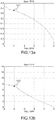
- the figure 6a represents the probability of detection as a function of the signal-to-noise ratio, for a probability of a false alarm of 10 -4 in a typical airborne case in the presence of ground clutter.
- the radar band is 2 MHz which provides 5 distance resolutions per pulse duration and 50 distance resolutions per recurrence.
- the figure 6a represents the map of ground echoes in distance and Doppler frequency in the sum channel of the antenna.
- a target is assumed to be in distance gate No. 32 and the Doppler filter No. 33 as shown in dotted lines, which is a location where the ground clutter is relatively large.
- the four curves shown on the figure 6b correspond to cases without pointing errors (curve 61), with a Doppler pointing error of 12.5% of filter width (curve 62), with errors of angular pointing in elevation and deposit of 34% and 17% opening respectively (curve 63), and with Doppler and angular pointing errors (curve 64).
- curve 61 cases without pointing errors
- curve 62 errors of angular pointing in elevation and deposit of 34% and 17% opening respectively
- curve 64 Doppler and angular pointing errors
- the probability of detection in this example tends to the value 0.8 due to ( 13 ).
- Doppler and / or angle errors in addition to the mismatch losses, the probability of detection quickly drops back to 0 without exceeding 0.1 in the worst case above.
- a simple approximation, for detection consists in replacing the parameters of the target (u, v, f) by the Doppler and angular hypotheses (u 0 , v 0 , f 0 ), as in the reference processing ( 8 ) for example.
- H is the single column matrix equal to C (u 0 , v 0 , f 0 ), calibrated at a certain level of quantification of the angular hypotheses for a given wavelength
- ⁇ is the function to a single component, constant and equal to 1. This is a “constant by pieces” approximation.
- the k u v f with the multivariate extension of the following Lagrange interpolator polynomials:
- the i u v f ⁇ r : u r ⁇ u i u - u r u i - u r ⁇ s : v s ⁇ v i v - v s v i - v s ⁇ t : f t ⁇ f i f - f t f i - f t i - f t
- Lagrange interpolation is a simple and direct way to approach the angular response of the network locally, requiring calibration of the antenna in a few reference angles around the viewing angle.
- a judicious choice by default is to take the roots of the Tchebychev polynomials [ 4 , 6 ] on each of the neighborhoods of the parameters taken individually, because this choice guarantees good approximation by limiting the maximum approximation error by a value tending rapidly to 0 with the number of interpolation points for a large class of functions. It is a choice which avoids being confronted with the Runge phenomenon [ 6 ] characterized by strong oscillations of the interpolating polynomials between two reference points.
- the disadvantage is to lose flexibility in the sampling of the angle / Doppler domain since the dimension of the approximation (ie the columns of H in ( 14 )) is the product of the dimensions of the spatial and temporal approximations (ie the columns of H s and H t in ( 24 )).
- Figures 7a, 7b , 8a and 8b represent the relative errors:
- the display dynamics were limited to the relative error of 10%.
- the matrix H r depends on the Doppler score f 0 .
- the collection of vectors X n given by ( 26 ) is then written: X 0 , ... , X NOT - The ⁇ ⁇ HB H r T + V 0 , ... , V NOT -
- B ⁇ u v f ⁇ r T f , which is a matrix function, generally non-linear, of the triplet of unknown parameters (u, v, f) associated with the target, and valid in the vicinity of the pointing (u 0 , v 0 , f 0 ).
- the identity matrix with the numerator and the denominator is of size equal to the number of columns of H r in ( 28 ), ie the dimension of approximation of the time stamping vector along the burst C r ( 27 ).
- Solution ( 30 ) has essentially two limitations. The first is that it does not provide optimal performance in terms of probability of detection, uniformly for all signal to noise values (test not uniformly more powerful [12]). The other limitation of ( 30 ) is linked to the degrees of freedom consumed by the approximations made via H and H r . In return for the robustness to angular and Doppler errors, the detection performance degrades all the more as the approximations are precise and the columns of H and H r numerous.
- the figure 9a illustrates the compromise between performance and robustness against ( 30 ) on a case where the target is present with the same Doppler as the ground echoes vertical to the carrier, case of the "altitude line", in the range door # 16 and the Doppler filter # 4 marked with white dotted lines on the figure 9a .
- the pointing vector is approached by Lagrange interpolation on 9 points and the time pointing vector C r at the scale of the burst ( 27 ) is approached by Taylor expansion in the 1st order.
- the MLED is seen as a kind of GLRT in two stages corresponding to a simplification of the GMLED, the latter being considered (without justification) as the GLRT of the detection problem without secondary data and without pointing errors formulated through ( 6 ).
- H C
- solution ( 30 ) is simplified by: VS 0 * S f 0 - 1 Z f 0 2 VS 0 * S f 0 - 1 VS 0 1 + Z f 0 * S f 0 - 1 Z f 0
- C 0 the pointing vector in the targeted direction C (u 0 , v 0 , f 0 ) and where Z f 0 in ( 31 ) has here only one column (it is a vector) .
- Expression ( 34 ) coincides with the GMLED detector reported in [ 15 ] for example.
- the equivalent expression ( 35 ) allows a more efficient implementation because the matrix R ⁇ is calculated and inverted only once while S f 0 in ( 34 ) is calculated and inverted for each Doppler hypothesis f 0 .
- the GMLED is indeed the GLRT of the detection problem without secondary data restricted to the case without pointing errors.
- AMF processing ( 8 ) the presence of a quadratic form in the denominator in ( 35 ) improves the robustness of the detector even with small pointing errors.
- the disadvantage, compared to ( 8 ), is the additional computation load which represents the quadratic form having to be evaluated for each Doppler frequency f 0 treated.
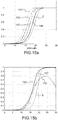
- the Figures 10a and 10b show a comparison of the performances between the AMF ( 8 ) and GMLED ( 35 ) detectors on the same scenario as the Figures 6a and 6b .
- the curves of the figure 10a are taken from the figure 6b for ease of reading.
- the GMLED detector without pointing errors has a probability of detection 101 which converges to 1 unlike the AMF where the latter 61 converges to 0.8.
- the robustness of the GMLED is clearly visible in the presence of Doppler errors which generate a loss of the order of dB, or angular 104 which generate a loss of a few dB (according to the SNR).
- the probability of detection 102 drops to 0 from an SNR of 60 dB.
- the GMLED is more robust than the AMF since the probability of detection 103 reaches 0.8 around 25 dB of SNR (whereas it does not exceed 0.1 with the AMF) but falls quickly to 0 for larger SNRs.
- the robustness of the GMLED is therefore better without being sufficient at medium / high signal to noise ratio.
- detectors without secondary data MLED and GMLED their higher sensitivity compared to detectors with secondary data, as well as their hyper-resolving properties, are studied theoretically and by simulations in [ 14 ] with complements in [ 16 ], as well than on real data in [ 17 ]. It appears in particular from this work that, in general, detectors without secondary data are less robust to pointing errors in Doppler than to angular errors. The pointing error on the angular part has more impact on the performance of the GMLED than on that of the MLED, but conversely the GMLED is more robust to pointing errors in Doppler compared to the MLED.
- the GMLED is more efficient at low SNR while the MLED prevails over the GMLED at high SNR.
- GIP criterion Generalized Inner Product
- ACE Adaptive Coherence Estimator
- the temporal part of the approximation is for example carried out by means of the matrix H r .
- the spatial part of the approximation is for example performed by the Lagrange interpolation.
- the new detectors thus defined are not uniformly more powerful. They significantly improve detection performance at medium / strong SNR but can be used in conjunction with other detectors. For example, the detector according to relation ( 30 ) being sometimes better at low SNR, it may be necessary to implement a mixed device between a detector according to ( 30 ) and TSA-MLED or ASA-MLED.
- C 0 being the pointing vector in the targeted direction C (u 0 , v 0 , f 0 ), u 0 , v 0 being the angular pointing hypotheses.
- the vector ⁇ r ( f ) in ( 28 ) has two components which are [1, (ff 0 )] T and the matrix Z f 0 in ( 31 ) or above in ( 37 ) also has two columns.
- the matrix S f 0 is always given by ( 33 ).
- the figure 11 shows schematically a preferred variant of TSA-MLED implementation.
- the angular pointing hypotheses (u 0 , v 0 ) of the vector C 0 make it possible to carry out the measurements 111 and to obtain the data cube X, according to the 3 characteristic dimensions of the radar, arranged according to ( 32 ).
- This data cube makes it possible to estimate the covariance 112 by calculating R ⁇ according to ( 10 ), as well as to calculate the two columns (vectors) z 1 and z 2 of the matrix Z f 0 by means of a Fourier transformation modified 113 described in ( 31 ) with the Doppler hypothesis f 0 and the approximation matrix H r of which ( 38 ) is a preferred variant.
- the Doppler hypothesis f 0 and the pointing angles (u 0 , v 0 ) moreover make it possible to calculate 116 the pointing vector C 0 , for the pointing in speed (calculation of the replica of the pointing vector C 0 ).
- the calculation 114 of the coefficients of the TSA-MLED is then carried out from the elements R ⁇ , z 1 , z 2 , and C 0 . More precisely, these coefficients are the parameters a 1 , a 2 , q 1 , q 2 , y, ⁇ and g obtained by equations ( 41 ) to ( 48 ), leading to the calculation of l TSA-MLED .
- Adaptive processing is applied by the TSA-MLED 115 filtering defined by l TSA-MLED . More particularly, the detector l TSA-MLED is compared with a given threshold.
- GMLED ( 35 ) and TSA-MLED ( 40 ) we want to avoid having to calculate and invert the matrix S f 0 for each Doppler hypothesis f 0 .
- the figure 12 schematizes a preferred and advantageous variant of implementation of ASA-MLED.
- several pointing vectors are used, that is to say several angular references.
- the angular pointing hypotheses make it possible to carry out the measurements and obtain the data cube X arranged according to ( 32 ). This last makes it possible to estimate 112 the covariance by calculating R ⁇ according to ( 10 ), as well as to calculate 122 the Fourier transform of the signal in each of the space-time channels via ( 9 ) with the Doppler hypothesis f 0 , giving the vector X f 0 .
- the Fourier transform is not extended, because we do not make the approximation on the burst.
- the Doppler hypothesis f 0 and the pointing angles (u 0 , v 0 ) moreover make it possible to calculate 121 the approximation matrix H of the pointing vector as described in a previous paragraph on taking into account pointing errors.
- the elements X f 0 , R ⁇ , and H then allow the calculation 123 of the coefficients of q 1 , q 2 of the ASA-MLED detector by equations ( 52 ) and ( 53 ).
- the adaptive processing is obtained by this filtering 124 (comparison of the detector l ASA-MLED to a given threshold).
- the opening of the antenna being for example 51 mrad in both directions, the relative angular pointing errors are 34% and 17% and the pointing error in Doppler is 40% (strong errors).
- the relative error between the pointing vector associated with the target and the pointing vector associated with the angular hypotheses tainted with errors is 36%.
- FIGS. 13a and 13b show the values of empirical thresholds estimated by Monte-Carlo draws as a function of the desired P fa , with 5.10 5 draws of the “temporal” GLRT ( 37 ) and TSA-MLED ( 39 ) detectors both implemented with Taylor interpolation .
- the threshold retained 131 for the GLRT ( figure 13a ) and the threshold retained 132 for TSA-MLED ( figure 13b ) are 0.66 and 7.27 respectively.
- the Figures 14a and 14b show the detection probabilities as a function of the SNR of the two detectors, GLRT and TSA-MLED.
- curves are represented on the same figure: they correspond to the case without errors (curve 141), with Doppler error only (curve 142), with angular error only (curve 143) and errors in angle and in Doppler (curve 144).
- the performances obtained in the sum channel are represented by a curve ⁇ .
- the two detectors clearly improve the performance of the GLRT ( 30 ) with approximations in the spatial and temporal domains (to be compared with the figure 9b ).
- the GLRT with approximation in the time domain ( figure 14a ) provides a maximum gain of more than 5 dB compared to the sum channel when there are no errors on the pointing vector, for all SNRs.
- it is very robust to pointing error in Doppler, since desensitization is negligible except at high SNR where it can reach around 2 dB.
- the proposed detector TSA-MLED shows a maximum gain compared to the sum channel a little less important ( ⁇ 4 dB) than the GLRT but a robustness to errors on the pointing vector much higher.
- the TSA-MLED makes it possible to conserve a gain of 2 to 3 dB from the weak SNR compared to the sum channel, up to the strong SNR.
- the performance of the APES Stop-Band would be a little better than that of the TSA-MLED: for example for an SNR of 15 dB the P d would be almost 0.6 against 0.4 on the figure 14b .
- the results are in favor of the TSA -MLED since the latter saves about 1.5 to 2 dB more than the APES Stop-Band compared to the sum channel for all SNRs.
- TSA-MLED and GLRT detectors are naturally complementary: neither is uniformly better than the other for all SNRs. At low / medium SNR it is the GLRT which wins while at medium / strong SNR it is the TSA-MLED.
- the latter can thus be used in combination with the GLRT to form a hybrid TSA-MLED / GLRT detector, at low cost in terms of computational load because the GLRT can be implemented in an optimized manner with the same quantities as those used.
- l there g ⁇ where y, g and ⁇ are given by ( 48 ), ( 45 ), and ( 47 ) respectively.
- the invention advantageously allows the estimation of angle pointing errors to take them into account in future pointing, in particular for the auto-calibration of the radar system.
Description
La présente invention concerne un procédé de détection adaptative d'une cible par un dispositif radar en présence d'interférences stationnaires. L'invention se situe notamment dans le domaine des radars aéroportés et des autodirecteurs de missiles mettant en œuvre des traitements adaptatifs spatio-temporels.The present invention relates to a method for adaptive detection of a target by a radar device in the presence of stationary interference. The invention is in particular in the field of airborne radars and missile seeker implementing adaptive space-time processing.
Les radars aéroportés ont pour mission de détecter des cibles en présence d'échos parasites et/ou de brouillage. Les échos de sol se retrouvent en angle et en distance, et en Doppler en raison du déplacement du porteur. Un traitement adaptatif spatio-temporel est un filtrage qui exploite les échos d'une antenne réseau à commande de phase sur plusieurs impulsions cohérentes. Un tel traitement permet la détection d'une cible se déplaçant à basse vitesse dans un fouillis de sol ou un brouillage électronique. Il analyse les variations spatiales et temporelles des échos. A la différence de méthodes de filtrage utilisant des algorithmes basés sur le premier ordre statistique des caractéristiques des échos, un traitement adaptatif spatio-temporel utilise le second ordre de ces statistiques. En effet, la détection d'une cible dans une porte distance n'est pas confinée à l'analyse des données dans cette porte distance mais utilise les données des portes distances adjacentes (données secondaires).
Ces traitements adaptatifs présentent cependant des inconvénients. En particulier, un problème à résoudre est la désensibilisation de ces traitements lorsqu'un signal utile provenant d'une cible est présent dans les données d'estimation de la fonction de corrélation des parasites. En effet, le signal utile est alors lui-même considéré comme un signal parasite.Airborne radars are responsible for detecting targets in the presence of parasitic echoes and / or interference. The ground echoes are found in angle and distance, and in Doppler due to the movement of the carrier. An adaptive spatio-temporal processing is a filtering which exploits the echoes of a network antenna with phase control on several coherent pulses. Such processing allows the detection of a target moving at low speed in a ground clutter or electronic jamming. It analyzes the spatial and temporal variations of the echoes. Unlike filtering methods using algorithms based on the first statistical order of the characteristics of the echoes, an adaptive spatio-temporal processing uses the second order of these statistics. Indeed, the detection of a target in a distance door is not confined to the analysis of the data in this distance door but uses the data of the adjacent distance doors (secondary data).
These adaptive treatments have drawbacks, however. In particular, a problem to be solved is the desensitization of these treatments when a useful signal originating from a target is present in the data for estimating the correlation function of the parasites. Indeed, the useful signal is then itself considered as a spurious signal.
Dans l'état de l'art ce problème est résolu en utilisant les portes distances voisines de la porte distance où est effectuée la détection. Cette solution n'est pas applicable aux formes d'ondes où une seule porte distance est disponible, par exemple avec des facteurs de formes élevés, supérieurs à 25%, et en absence de modulations. Quand elle est applicable, la solution est mise en défaut principalement dans les deux cas de figure suivants :
- Les parasites dans les données d'estimation ne sont pas suffisamment représentatifs de ceux de la porte distance sous test, ce qui arrive notamment avec les formes d'onde présentant beaucoup d'ambiguïtés en distance ou dans certaines zones des cartes de mesures du radar ;
- Le rapport signal à bruit est suffisamment élevé pour générer des lobes secondaires en distance qui ne sont pas négligeables dans les données d'estimation.
D'autres approches dites « sans données secondaires » ou « à unique jeu de données » proposent des traitements qui résolvent partiellement le problème. Avec ces approches, la désensibilisation du radar reste importante, notamment à moyen ou fort rapport signal à bruit et en présence d'erreurs, même faibles, de pointage angulaire du radar sur la cible, d'hypothèse Doppler ou de calibrage du réseau.
Un
- The parasites in the estimation data are not sufficiently representative of those of the distance gate under test, which happens in particular with waveforms having a lot of ambiguities in distance or in certain areas of the radar measurement maps;
- The signal to noise ratio is high enough to generate side lobes in distance which are not negligible in the estimation data.
Other approaches called “without secondary data” or “with a single data set” propose treatments which partially solve the problem. With these approaches, the desensitization of the radar remains important, in particular at medium or high signal to noise ratio and in the presence of errors, even small, of angular pointing of the radar on the target, of Doppler hypothesis or of network calibration.
A
Un but de l'invention est notamment de pallier les inconvénients précités.
A cet effet, l'invention a pour objet un procédé de détection adaptative d'une cible par un dispositif radar en présence d'interférences stationnaires, ledit radar étant équipé d'une antenne réseau, le procédé comportant :
- une étape de détermination d'un ensemble de vecteurs de pointage décrivant chacun une hypothèse d'arrivée angulaire et une hypothèse de pointage Doppler d'un signal utile reçu ;
- pour chaque vecteur de pointage, une étape d'approximation d'un signal utile reçu dans un voisinage en angle et en Doppler autour dudit vecteur produisant un modèle spatio-temporel approximé au voisinage de chacun desdits vecteurs de pointage ;
- une étape de détection par comparaison, avec un seuil donné, d'une caractéristique statistique d'un signal reçu de ladite cible au voisinage d'un vecteur de pointage avec le modèle spatio-temporel correspondant audit voisinage ;
To this end, the subject of the invention is a method of adaptive detection of a target by a radar device in the presence of stationary interference, said radar being equipped with a network antenna, the method comprising:
- a step of determining a set of pointing vectors each describing an angular arrival hypothesis and a Doppler pointing hypothesis of a useful signal received;
- for each pointing vector, a step of approximating a useful signal received in an angle and Doppler vicinity around said vector producing an approximate space-time model in the vicinity of each of said pointing vectors;
- a step of detection by comparison, with a given threshold, of a statistical characteristic of a signal received from said target in the vicinity of a pointing vector with the space-time model corresponding to said neighborhood;
ledit modèle étant temporel, ladite caractéristique statistique, notée ℓTSA-MLED, étant définie comme suit : ![]()
![]()
![]()
![]()
![]()
![]()
![]()
![]()
![]()
- C 0 étant le vecteur de pointage défini par ses hypothèses angulaires (u0, v0) et son hypothèse de pointage Doppler (f0) ;
- R̂ étant la matrice de covariance estimée des données spatio-temporelles X du signal reçu ;
- z1 et z2 étant les deux colonnes de la
matrice 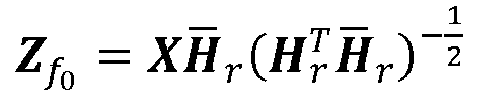
- H r étant une matrice d'approximation à deux colonnes, la première colonne étant constituée des composantes dudit développement de Taylor au premier ordre de l'hypothèse de pointage Doppler f0 et la deuxième colonne étant constituée des composantes de la dérivée par rapport à la fréquence audit pointage Doppler.
- C 0 being the pointing vector defined by its angular hypotheses (u 0 , v 0 ) and its Doppler pointing hypothesis (f 0 );
- R̂ being the estimated covariance matrix of the space-time data X of the received signal;
- z 1 and z 2 being the two columns of the
matrix - H r being a two-column approximation matrix, the first column consisting of the components of said first-order Taylor expansion of the Doppler pointing hypothesis f 0 and the second column consisting of the components of the derivative with respect to the frequency of Doppler scoring.
Ladite caractéristique statistique est par exemple basée sur l'estimation du maximum de vraisemblance. L'approximation spatiale au voisinage d'un vecteur de pointage est par exemple effectuée par une interpolation de Lagrange dudit vecteur. L'approximation temporelle au voisinage d'un vecteur de pointage est par exemple obtenue par un développement de Taylor au premier ordre de l'hypothèse de pointage Doppler dudit vecteur.Said statistical characteristic is for example based on the estimation of the maximum likelihood. The spatial approximation in the vicinity of a pointing vector is for example carried out by a Lagrange interpolation of said vector. The temporal approximation in the vicinity of a pointing vector is for example obtained by a first order Taylor expansion of the Doppler pointing hypothesis of said vector.
Ladite caractéristique statistique, notée ℓASA-MLED, peut être également définie comme suit : ![]()
![]()
![]()
- R̂ étant la matrice de covariance estimée des données spatio-temporelles X du signal reçu ;
-
X f0 est la transformée de Fourier en l'hypothèse de pointage Doppler f0 ; - H est une matrice d'approximation obtenue par approximation comme définie précédemment.
- R̂ being the estimated covariance matrix of the space-time data X of the received signal;
-
X f 0 is the Fourier transform in the Doppler pointing hypothesis f 0 ; - H is an approximation matrix obtained by approximation as defined above.
L'invention a également pour objet un radar aéroporté et/ou un autodirecteur de missile aptes à mettre en œuvre un tel procédé.The invention also relates to an airborne radar and / or a missile seeker capable of implementing such a method.
D'autres caractéristiques et avantages de l'invention apparaîtront à l'aide de la description qui suit, faite en regard de dessins annexés qui représentent :
- La
figure 1 , une structure d'antenne à 8 sous-réseaux ; - La
figure 2 , des valeurs du rapport signal à fouillis pour 100 tirages d'échos de sol ; - La
figure 3 , la densité empirique de test avec une cible de SNR de 100 dB et une valeur typique de seuil ; - La
figure 4 , la densité empirique de test, pour un SNR de 100 dB, la cible étant décalée en vitesse d'1/4 de filtre (visée et cible dans l'axe) ; - La
figure 5 , la densité empirique de test avec une cible de SNR de 100 dB, décalée en angle (visée dans l'axe) ; - Les
figures 6a et 6b , respectivement une carte des échos de sol en distance/Doppler dans la voie somme et la probabilité de détection en fonction du SNR pour AMF sans données secondaires ; - Les
figures 7a et 7b , respectivement des erreurs relatives d'interpolation constante et linéaire ; - Les
figures 8a et 8b , respectivement des erreurs relatives d'interpolation deLagrange 4 points et 9 points ; - Les
figures 9a et 9b , respectivement une carte des échos de sol en distance/Doppler dans la voie somme et la probabilité de détection en fonction du SNR ; - Les
figures 10a et 10b , respectivement les performances AMF et GMLED ; - La
figure 11 , un schéma d'une première mise en œuvre du TSA-MELD ; - La
figure 12 , un schéma d'une deuxième mise en œuvre du TSA-GMLED ; - Les
figures 13a et 13b , la relation empirique du seuil par rapport à la probabilité de fausse alarme Pfa estimée sur 5.105 tirages pour un détecteur GLRT temporel et pour un détecteur TSA- MELD ; - Les
figures 14a et 14b , la probabilité de détection Pd en fonction du SNR pour un détecteur GLRT temporel et pour un détecteur TSA- MELD ; - Les
figures 15a et 15b , Pd en fonction du SNR pour un détecteur du type « Stop-Band APES », et pour des détecteurs GLRT, TSA-MLED et hybride.
- The
figure 1 , an antenna structure with 8 sub-networks; - The
figure 2 , values of the signal-to-clutter ratio for 100 ground echo prints; - The
figure 3 , the empirical test density with an SNR target of 100 dB and a typical threshold value; - The
figure 4 , the empirical test density, for an SNR of 100 dB, the target being shifted in speed by 1/4 of the filter (aim and target in the axis); - The
figure 5 , the empirical test density with an SNR target of 100 dB, offset in angle (aimed in the axis); - The
Figures 6a and 6b , respectively a map of the ground echoes in distance / Doppler in the sum channel and the probability of detection as a function of the SNR for AMF without secondary data; - The
Figures 7a and 7b , respectively relative errors of constant and linear interpolation; - The
Figures 8a and 8b , respectively 4-point and 9-point lagrange interpolation errors; - The
Figures 9a and 9b , respectively a map of distance / Doppler ground echoes in the sum channel and the probability of detection as a function of the SNR; - The
Figures 10a and 10b , respectively AMF and GMLED performance; - The
figure 11 , a diagram of a first implementation of the TSA-MELD; - The
figure 12 , a diagram of a second implementation of the TSA-GMLED; - The
Figures 13a and 13b , the empirical relation of the threshold compared to the probability of false alarm P fa estimated on 5.10 5 draws for a temporal GLRT detector and for a TSA-MELD detector; - The
Figures 14a and 14b , the probability of detection P d as a function of the SNR for a temporal GLRT detector and for a TSA-MELD detector; - The
Figures 15a and 15b , P d as a function of the SNR for a “Stop-Band APES” type detector, and for GLRT, TSA-MLED and hybrid detectors.
Avant de décrire plus en détail l'invention, on commence par exposer de façon plus précise le problème de la détection adaptative sans données secondaires. Dans un premier temps on définit les notations employées par la suite, puis on montre les limites d'un traitement standard de détection adaptative sans données secondaires quand le pointage sur la cible est imparfait.Before describing the invention in more detail, we begin by explaining more precisely the problem of adaptive detection without secondary data. First, we define the notations used by next, then we show the limits of a standard adaptive detection processing without secondary data when the aiming on the target is imperfect.
On considère un radar à antenne active avec P voies spatiales de réception. Pour fixer les idées, on peut considérer l'exemple de la découpe spatiale amsar issue de [1] où P voies sont réparties sur une surface rayonnante approximativement circulaire de diamètre 60cm, comme illustré sur la
Après filtrage et échantillonnage à la bande passante du radar, le signal Y n à la récurrence n dans une porte distance s'écrit : ![]()
- N est le nombre d'impulsions ;
- α est l'amplitude complexe (inconnue) de la cible ;
- G est le vecteur des gains complexes des sous-réseaux dans la direction de la cible ;
- v est la fréquence Doppler associée à la cible ;
- Tr est la période de récurrence des impulsions et ;
- W n est le signal des échos de sol classiquement supposé Gaussien, centré, et stationnaire, sa matrice d'autocorrélation étant notée Q 0 .
- N is the number of pulses;
- α is the complex (unknown) amplitude of the target;
- G is the vector of the complex gains of the subnets in the direction of the target;
- v is the Doppler frequency associated with the target;
- T r is the period of recurrence of the pulses and;
- W n is the signal for ground echoes classically assumed to be Gaussian, centered, and stationary, its autocorrelation matrix being noted Q 0 .
La modélisation habituelle des échos de sol comprend la corrélation temporelle d'impulsion à impulsion des retours de sol, supposés stationnaires. La matrice de corrélation entre W n et W n+s est notée Q δ et ne dépend pas de l'indice temporel n. Si on désigne par P le nombre de sous réseaux (par exemple P=8), les vecteurs Y n, G et W n sont de taille P et les matrices Q 0, Q δ sont de taille PxP. Dans le cas d'un brouillage à bruit, le signal d'interférence est habituellement supposé dé-corrélé temporellement ce qui signifie que dans ce cas Q δ = 0 pour δ >0.The usual modeling of ground echoes includes the temporal pulse-to-pulse correlation of ground returns, supposed to be stationary. The correlation matrix between W n and W n + s is noted Q δ and does not depend on the time index n . If we denote by P the number of sub-networks (for example P = 8), the vectors Y n , G and W n are of size P and the matrices Q 0 , Q δ are of size PxP. In the case of noise interference, the interference signal is usually assumed to be temporally uncorrelated, which means that in this case Q δ = 0 for δ> 0.
Pour prendre en compte les corrélations temporelles des échos parasites tels que les échos de sol, on se donne classiquement un horizon temporel glissant de L récurrences au-delà duquel on néglige la corrélation des retours de sol. Généralement L est très inférieur à N (L<<N), L étant généralement de l'ordre de la dizaine voire moins alors que N est de l'ordre de la centaine voire plus. Les données spatio-temporelles X n dans cet horizon sont constituées des vecteurs (Y n, ..., Y N+L-1) concaténés en un seul vecteur de taille PL : ![]()
![]()
On définit de même le vecteur de pointage (« steering vector ») spatio-temporel, C, et la matrice d'autocorrélation spatio-temporelle associée au fouillis, Q, avec une notation par blocs : ![]()

![]()
De même les échantillons spatio-temporels de fouillis sont (V 0, ..., V N-L) tels que : ![]()
![]()
![]()
![]()
Avec une fenêtre glissante de taille L, les vecteurs spatio-temporels X n sont au nombre de (N-L+1). Dans toute la suite on notera N' = N-L+1. Le vecteur de pointage C dépend de la direction (u,v) de la cible et de son Doppler v. Cette dépendance peut être explicitée en écrivant C = C(u,v,f) où par commodité on note f la fréquence Doppler ramenée au pas de quantification (NTr)-1 en fréquence, soit ![]()
![]()
Pour des hypothèses angulaires (u0, v0) et une hypothèse Doppler f0/(NTr), avec f0 = 0,...,N-1, le traitement classique consiste à comparer le nombre T suivant à un seuil : où ![]()
![]()
![]()
![]()
![]()
![]()
A un facteur constant près, le test de référence correspond au test obtenu en supposant connaître la matrice d'autocorrélation Q (cf.(4)) puis en lui substituant une estimation R̂ au sens du maximum de vraisemblance. C'est un traitement du type rapport de vraisemblance généralisé en deux étapes connu dans les publications sous le nom de « Adaptive Matched Filter » (AMF) [2] dans le cas où des données secondaires d'estimation de Q sont disponibles en nombre suffisant.With a constant constant factor, the reference test corresponds to the test obtained by supposing to know the autocorrelation matrix Q (cf. ( 4 )) then by substituting for it an estimate R̂ in the sense of maximum likelihood. It is a treatment of the generalized likelihood ratio type in two stages known in the publications under the name of “ Adaptive Matched Filter” (AMF) [ 2 ] in the case where secondary data of estimation of Q are available in sufficient number .
Ici, on se place dans une application du traitement AMF « sans données secondaires » puisqu'on utilise les mêmes données pour estimer Q et tester la présence d'une cible. Cette approche est pertinente en particulier dans les modes air/air très ambigus en distance pour lesquels la matrice Q n'est pas homogène d'une porte distance à l'autre (les données d'une porte distance ne pouvant alors pas être utilisées pour estimer Q dans une autre porte distance), ou encore dans certains autodirecteurs de missiles où les formes d'onde sont telles qu'une seule porte distance est disponible pour assurer les boucles de poursuite.Here, we place ourselves in an application of AMF processing "without secondary data" since we use the same data to estimate Q and test the presence of a target. This approach is relevant in particular in very ambiguous air / air modes in distance for which the matrix Q is not homogeneous from one distance door to another (the data from a distance door cannot then be used to estimate Q in another range), or in some missile seekers where the shapes waveforms are such that only one distance gate is available to provide tracking loops.
La cible doit avoir une puissance faible par rapport à la puissance des parasites pour permettre en première approximation de négliger sa contribution dans l'estimation de Q. Cette hypothèse est généralement vérifiée pour des cibles usuelles à moyenne ou grande distance. Cependant, l'approche ci-dessus atteint ses limites quand la puissance de la cible devient grande et que les paramètres de la cible (u,v,f) ne sont pas exactement égaux aux hypothèses Doppler et angulaire (u0,v0,f0), ce qui est toujours le cas en pratique.The target must have a low power compared to the power of the parasites to allow as a first approximation to neglect its contribution in the estimation of Q. This assumption is generally verified for usual targets at medium or long distance. However, the above approach reaches its limits when the power of the target becomes large and the parameters of the target (u, v, f) are not exactly equal to the Doppler and angular hypotheses (u 0 , v 0 , f 0 ), which is always the case in practice.
A titre d'illustration, on suppose dans un premier temps que les hypothèses Doppler et angulaires du traitement coïncident exactement avec les paramètres de la cible, et que le vecteur de pointage C est parfaitement connu (calibré). Dans ce cas particulier, on peut calculer le rapport entre la puissance du signal cible et la puissance du signal de parasite (rapport signal à fouillis). On montre que celui-ci est une fonction F de l'amplitude complexe α de la cible, du vecteur de pointage C = C(u,v,f) = C(u0,v0,f0), de la transformée de Fourier ![]()
![]()
![]()
![]()
Si on s'intéresse au cas où la puissance de la cible devient très grande, c'est à dire quand |α|2 → ∞, on montre que le rapport signal à fouillis F tend vers la valeur suivante qui est non nulle : 
Par exemple la ![]()
![]()
Les valeurs calculées des deux manières coïncident ce qui permet de valider (13). On s'aperçoit que les plus petites valeurs sont de l'ordre de 4 dB ce qui doit permettre de conserver une bonne probabilité de détection aux Pfa (probabilité de fausses alarmes) usuelles.The values calculated in the two ways coincide, which makes it possible to validate ( 13 ) . It can be seen that the smallest values are of the order of 4 dB, which must make it possible to maintain a good probability of detection at the usual P fa (probability of false alarms).
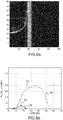
La
Sur l'histogramme on indique de plus en traits pointillés 31 une valeur typique de seuil de détection sur bruit thermique, correspondant à une probabilité de fausse alarme de 10-4 (soit un seuil de 0.23 calculé par ailleurs). On constate que dans la majorité des cas la cible est détectée. Un calcul plus précis montre que sur cet exemple la probabilité de détection est de 0.998, ce qui est une désensibilisation négligeable due à la présence de la cible.On the histogram, a dotted
Les résultats précédents sont valables quand le vecteur de pointage C est parfaitement connu. En pratique ce n'est pas le cas, d'une part en raison de la quantification des paramètres angulaires et Doppler (la position de la cible n'est jamais exactement une des valeurs quantifiées pour faire le test de détection), et d'autre part en raison d'un calibrage plus ou moins bon du réseau qui implique une incertitude sur les gains complexes des sous-réseaux. Quand le vecteur de pointage associé à la cible diffère légèrement du vecteur de pointage utilisé pour détecter, la perte de performance n'est plus négligeable comme le montre l'exemple illustré par la
Si on suppose que la cible, de SNR 100 dB, est décalée en vitesse d'un quart de filtre Doppler par rapport à l'hypothèse Doppler du radar (f = f0 + 1/4), on obtient la densité empirique du test (8) représentée par cette
La même valeur de seuil 31 que sur la
La valeur du seuil n'est pas indiquée sur la
Enfin, la
La
Les quatre courbes représentées sur la
Pour conserver les avantages de l'approche sans données secondaires, il faut tenir compte des erreurs de pointage dans la modélisation du signal, de manière à limiter le plus possible les pertes associées. Dans les lignes qui suivent, on explique un moyen général d'y parvenir, avec les traitements existants et leurs limitations.To keep the advantages of the approach without secondary data, it is necessary to take into account the errors of pointing in the modeling of the signal, in order to limit as much as possible the associated losses. In the following lines, we explain a general way to achieve this, with existing treatments and their limitations.
Comme cela sera décrit par la suite, pour tenir compte des erreurs de pointage, la solution selon l'invention consiste à remplacer, dans le modèle classique (1) ou (6), le vecteur de pointage C, vu comme une fonction vectorielle inconnue, par une approximation locale bien choisie. En fonction des conditions d'utilisation de l'invention et des moyens de calibrage, entre autres, différents choix sont possibles. D'une manière générale, l'approximation de C s'écrit sous la forme suivante, dans un voisinage V(u0,v0,f0) des hypothèses (u0,v0,f0) : ![]()
- une matrice H connue et fixée à l'avance, soit par modélisation ou calcul, soit par calibrage du réseau antennaire (à coût significativement moindre que la calibration de la totalité de la fonction C), et ;
- une fonction vectorielle φ dont le nombre de composantes est généralement beaucoup plus petit que celui de C et dont la forme (i.e. l'expression analytique) est connue.
- a matrix H known and fixed in advance, either by modeling or calculation, or by calibration of the antenna array (at significantly lower cost than the calibration of the entire function C ), and;
- a vector function φ whose number of components is generally much smaller than that of C and whose form (ie the analytical expression) is known.
Par exemple, une approximation simple, pour la détection, consiste à remplacer les paramètres de la cible (u,v,f) par les hypothèses Doppler et angulaires (u0,v0,f0), comme dans le traitement de référence (8) par exemple. Dans ce cas, H est la matrice à une seule colonne égale à C(u0,v0,f0), calibrée à un certain niveau de quantification des hypothèses angulaires pour une longueur d'onde donnée, et φ est la fonction à une seule composante, constante et égale à 1. Il s'agit d'une approximation « constante par morceaux ».For example, a simple approximation, for detection, consists in replacing the parameters of the target (u, v, f) by the Doppler and angular hypotheses (u 0 , v 0 , f 0 ), as in the reference processing ( 8 ) for example. In this case, H is the single column matrix equal to C (u 0 , v 0 , f 0 ), calibrated at a certain level of quantification of the angular hypotheses for a given wavelength, and φ is the function to a single component, constant and equal to 1. This is a “constant by pieces” approximation.
Une autre approximation qui peut être faite, pour les mesures d'écartométries angulaires, consiste à substituer à C(u,v,f) son développement de Taylor au voisinage des hypothèses (u0,v0,f0), comme dans [3] par exemple. Si on néglige l'erreur de Doppler (f≈f0), H est une matrice à 3 colonnes : ![]()

![]()
Si on veut prendre en compte les erreurs Doppler, il suffit de rajouter les éléments correspondants dans une quatrième colonne de H et une quatrième composante de φ. Avec P=8 voies et L=6 retards, le vecteur de pointage C a 48 composantes alors que φ n'en a qu'au plus 4. L'avantage de l'approximation de Taylor est son caractère linéaire : la linéarité de la fonction φ la rend simple à inverser pour retrouver les mesures d'écartométries à partir d'une estimation de φ. Son inconvénient est que l'approximation devient trop grossière sur les bords de l'ouverture d'antenne. C'est pourquoi d'autres approximations peuvent être envisagées. Par exemple, si on veut une erreur d'approximation nulle pour k+1 hypothèses prédéfinies (u0,v0,f0), ..., (uk,vk,fk) dans le voisinage V(u0,v0,f0), une approximation intéressante est l'interpolation de Lagrange [4]. Dans ce cas la matrice H possède k+1 colonnes qui sont les vecteurs de pointage calibrés aux k+ 1 hypothèses de référence : ![]()

![]()
![]()
![]()
L'interpolation de Lagrange est une manière simple et directe d'approcher localement la réponse angulaire du réseau, nécessitant le calibrage de l'antenne en quelques angles de référence autour de l'angle de visée. En absence de contrainte ou de préconisation particulière sur le choix des points de référence, un choix judicieux par défaut est de prendre les racines des polynômes de Tchebychev [4,6] sur chacun des voisinages des paramètres pris individuellement, car ce choix garantit une bonne approximation en bornant l'erreur maximale d'approximation par une valeur tendant rapidement vers 0 avec le nombre de points d'interpolation pour une large classe de fonctions. C'est un choix qui évite d'être confronté au phénomène de Runge [6] caractérisé par de fortes oscillations des polynômes interpolateurs entre deux points de référence. Les racines des polynômes de Tchebychev sont explicites - on montre que pour k+1 points d'interpolation sur [-1 ; 1] elles sont égales à ![]()
![]()
Un autre choix possible provient du fait que la réponse d'une cible en fréquence Doppler est plus particulière et mieux connue que la réponse angulaire du réseau car elle correspond à un déphasage d'impulsion à impulsion crée par la cinématique entre le radar et la cible [8]. On peut ainsi séparer le paramètre f des paramètres angulaires u et ven notant : ![]()
![]()
![]()
![]()
Sa taille est le nombre L de retards. En approchant les approximations temporelles et spatiales de manière similaire à (14) : ![]()
![]()
![]()
![]()
![]()
![]()
![]()
![]()
L'avantage de séparer les paramètres de fréquence et d'angles permet d'utiliser des méthodes d'approximation adaptées à chacune des composantes C t et C s. Ainsi, l'interpolation de Lagrange se prête bien à une calibration de la réponse mal connue C s du réseau en quelques points de visée, alors que la forme connue de C t (au paramètre f près) permet une approximation par des méthodes optimales, comme par exemple le développement de Karhunen-Loève [9] si on cherche une approximation optimale en moindre carrés. L'inconvénient est de perdre en souplesse dans l'échantillonnage du domaine angle/Doppler puisque la dimension de l'approximation (i.e. les colonnes de H dans (14)) est le produit des dimensions des approximations spatiale et temporelle (i.e. les colonnes de H s et H t dans (24)).The advantage of separating the frequency and angle parameters makes it possible to use approximation methods adapted to each of the components C t and C s . Thus, the Lagrange interpolation lends itself well to a calibration of the poorly known response C s of the network at a few points of target, while the known form of C t (with the parameter f close) allows an approximation by optimal methods, such as for example the development of Karhunen-Loève [ 9 ] if one seeks an optimal approximation in least squares. The disadvantage is to lose flexibility in the sampling of the angle / Doppler domain since the dimension of the approximation (ie the columns of H in ( 14 )) is the product of the dimensions of the spatial and temporal approximations (ie the columns of H s and H t in ( 24 )).
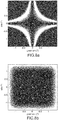
Pour illustrer l'approximation du la partie spatiale C s du vecteur de pointage, les
Sur la
Si on reporte l'approximation locale (14) du vecteur de pointage C dans le modèle du signal reçu (6), on obtient : ![]()
![]()
![]()
![]()
![]()
![]()
De même que H t dans (22), la matrice H r dépend du pointage Doppler f0 . La collection des vecteurs X n donnés par (26) s'écrit alors : ![]()
![]()
![]()
![]()
Le problème de détection qu'on veut résoudre consiste alors à tester la nullité du paramètre complexe inconnu α dans (29), pour des paramètres (u,v,f) dans un voisinage d'une hypothèse (u0,v0,f0), et avec un signal parasite (V n)n=0...N-L Gaussien complexe centré de matrice d'autocorrélation Q inconnue.The detection problem that we want to solve then consists in testing the nullity of the unknown complex parameter α in ( 29 ), for parameters (u, v, f) in the vicinity of a hypothesis (u 0 , v 0 , f 0 ), and with a parasitic signal ( V n ) n = 0 ... N - L Gaussian complex centered with unknown autocorrelation matrix Q.
Formulé par l'intermédiaire de (29), le problème technique rentre dans le cadre très général de la détection de signaux multidimensionnels, traité en profondeur dans un travail de Kelly en 1989 [10] basé sur le principe du rapport de vraisemblance généralisé (GLRT, Generalized Likelihood Ratio Test) [11]. Sous l'hypothèse (fausse mais nécessaire pour surmonter les difficultés d'établissement d'un traitement de détection) que les vecteurs de fouillis de sol V 0 , ..., V N-L sont indépendants, la solution générale consiste à comparer le quotient de déterminants ci-dessous à un seuil : ![]()
![]()
Dans l'expression ci-dessus la matrice identité au numérateur et au dénominateur est de taille égale au nombre de colonnes de H r dans (28), i.e. la dimension d'approximation du vecteur de pointage temporel le long de la rafale C r (27). La matrice Z f0 est une sorte de généralisation de la transformée de Fourier des données au voisinage de l'hypothèse Doppler f0 : ![]()
![]()
![]()
![]()
Sa dépendance au pointage Doppler f0 est due à la matrice H r elle-même dépendante de f0 . De même, la matrice S f0 est une sorte d'estimation de l'autocorrélation des données : ![]()
![]()
Enfin, la matrice P au dénominateur de (30) apparaît dans les calculs reportés dans [10] et son expression réalise une sorte de couplage entre l'approximation du vecteur de pointage C (via H) et l'approximation du vecteur de pointage temporel C r le long de la rafale (via H r dans S f0) : ![]()
![]()
Son expression est implicitement dépendante de la visée (u0,v0,f0) par l'intermédiaire de H.Its expression is implicitly dependent on the target (u 0 , v 0 , f 0 ) via H.
La solution (30) a essentiellement deux limitations. La première est qu'elle ne fournit pas les performances optimales en termes de probabilité de détection, uniformément pour toutes les valeurs de signal à bruit (test non uniformément plus puissant [12]). L'autre limitation de (30) est liée aux degrés de liberté que consomment les approximations effectuées via H et H r. En contrepartie de la robustesse aux erreurs angulaires et Doppler, les performances de détection se dégradent d'autant plus que les approximations sont précises et les colonnes de H et H r nombreuses. La
Sur la
Un lien intéressant peut être établi entre (30) et une grande part des travaux sur la détection sans données secondaires réalisés par Aboutanious et Mulgrew à la fin des années 2000, reportés dans les références [13] à [18]. On y trouve l'étude détaillée de deux détecteurs, basée sur l'estimation du maximum de vraisemblance pour l'un, noté MLED (Maximum Likelihood Estimation Detector) et basé sur l'estimation du maximum de vraisemblance généralisé pour l'autre, noté GMLED (Generalized Maximum Likelihood Estimation Detector). Tous deux sont présentés comme des détecteurs du GLRT dans le cas simplifié où l'on ne tient pas compte des erreurs de pointage. Le MLED est vu comme une sorte de GLRT en deux temps correspondant à une simplification du GMLED, ce dernier étant considéré (sans justification) comme le GLRT du problème de détection sans données secondaire et sans erreurs de pointage formulées par l'intermédiaire de (6). Si l'on replace la modélisation (29) dans le cas où il n'y a pas d'erreurs de pointage, on a avec les notations précédentes H = C, B = 1, Hr = Cr, et après quelques calculs élémentaires on montre que la solution (30) se simplifie en : 
![]()
![]()
![]()
![]()
![]()
![]()
L'expression (34) coïncide avec le détecteur GMLED reporté dans [15] par exemple. L'expression équivalente (35) permet une mise en œuvre plus efficace car la matrice R̂ n'est calculée et inversée qu'une seule fois alors que S f0 dans (34) est calculée et inversée pour chaque hypothèse Doppler f0 . Ainsi, le GMLED est bien le GLRT du problème de détection sans données secondaire restreint au cas sans erreurs de pointage. Par rapport au traitement AMF (8), la présence d'une forme quadratique au dénominateur dans (35) permet d'améliorer la robustesse du détecteur même avec de petites erreurs de pointage. L'inconvénient, par rapport à (8), est la charge de calcul supplémentaire que représente la forme quadratique devant être évaluée pour chaque fréquence Doppler f0 traitée. Les
Sur la
Une variante simplifiée du détecteur GMLED, le MLED (Maximum Likelihood Estimator Detector) a également été proposée et étudiée dans [13-18]. Son expression est établie dans [13] à partir de travaux antérieurs sur l'algorithme APES (Amplitude and Phase EStimation) pour l'estimation spectrale en imagerie radar [20], basés sur le critère des moindres carrés. Elle est similaire à (34) où la forme quadratique du dénominateur est supprimée : 
Les performances des détecteurs sans données secondaires MLED et GMLED, leur sensibilité plus forte par rapport aux détecteurs avec données secondaires, ainsi que leurs propriétés hyper-résolvantes, sont étudiées théoriquement et par simulations dans [14] avec des compléments dans [16], ainsi que sur données réelles dans [17]. Il ressort notamment de ces travaux que, d'une manière générale, les détecteurs sans données secondaires sont moins robustes aux erreurs de pointage en Doppler qu'aux erreurs angulaires. L'erreur de pointage sur la partie angulaire a plus d'impact sur les performances du GMLED que sur celles du MLED, mais inversement le GMLED est plus robuste aux erreurs de pointage en Doppler par rapport au MLED. Avec des erreurs de pointage dans les deux domaines angulaires et Doppler, le GMLED est plus performant à faible SNR alors que le MLED l'emporte sur le GMLED à fort SNR.
Quand des données secondaires sont disponibles mais ne sont pas rigoureusement homogènes aux données testées, une approche combinant la détection avec et sans données secondaires a été proposée dans [15] et [18]. L'approche est basée sur l'utilisation du critère GIP (Generalized Inner Product) comme mesure d'hétérogénéité [21] entre données testées et données secondaires, et constitue une alternative à d'autres détecteurs comme ACE (Adaptive Coherence Estimator) [22] ou son extension multidimensionnelle [23] qui possèdent des propriétés d'invariance et d'optimalité dans des cas d'hétérogénéité particuliers [24- 26].The performance of detectors without secondary data MLED and GMLED, their higher sensitivity compared to detectors with secondary data, as well as their hyper-resolving properties, are studied theoretically and by simulations in [ 14 ] with complements in [ 16 ], as well than on real data in [ 17 ]. It appears in particular from this work that, in general, detectors without secondary data are less robust to pointing errors in Doppler than to angular errors. The pointing error on the angular part has more impact on the performance of the GMLED than on that of the MLED, but conversely the GMLED is more robust to pointing errors in Doppler compared to the MLED. With pointing errors in both areas angular and Doppler, the GMLED is more efficient at low SNR while the MLED prevails over the GMLED at high SNR.
When secondary data are available but are not strictly consistent with the data tested, an approach combining detection with and without secondary data has been proposed in [ 15 ] and [ 18 ]. The approach is based on the use of the GIP criterion ( Generalized Inner Product ) as a measure of heterogeneity [ 21 ] between tested data and secondary data, and constitutes an alternative to other detectors such as ACE ( Adaptive Coherence Estimator ) [ 22 ] or its multidimensional extension [ 23 ] which have invariance and optimality properties in particular cases of heterogeneity [ 24 - 26 ].
Compte tenu des limitations des détecteurs sans données secondaires en présence d'erreurs de pointage, une manière de prendre ces dernière en compte dans le MLED est décrite dans [27,28] avec le détecteur SB-APES (Stop-Band APES). Partant d'une interprétation du MLED comme une minimisation d'énergie dans un sous-espace, l'approche consiste à compenser les propriétés d'hyper-résolution en interpolant le vecteur de pointage temporel (27) à l'échelle de la rafale C r par interpolation de Lagrange en 3 points que sont le Doppler testé et ses demi-résolutions supérieures et inférieures. En reprenant la démarche de minimisation d'énergie avec l'interpolation de C r, les auteurs parviennent à un détecteur similaire au MLED (36) avec une matrice S f0 modifiée. L'approche a montré des résultats prometteurs sur données synthétiques bien qu'elle ne parvienne pas à éliminer entièrement les échos de sol. Elle a été étendue récemment dans [29] pour prendre en compte les aspects déterministes de la relation angle-Doppler vérifiée par les échos de sol, afin notamment de garantir une bonne maîtrise de la fausse alarme.Given the limitations of detectors without secondary data in the presence of pointing errors, a way of taking these into account in the MLED is described in [ 27 , 28 ] with the detector SB-APES ( Stop-Band APES ). Starting from an interpretation of MLED as a minimization of energy in a subspace, the approach consists in compensating for the properties of hyper-resolution by interpolating the time-stamping vector ( 27 ) on the scale of the burst C r by Lagrange interpolation at 3 points which are the Doppler tested and its upper and lower half-resolutions. Using the energy minimization approach with the interpolation of C r , the authors arrive at a detector similar to MLED ( 36 ) with a modified S f 0 matrix. The approach has shown promising results on synthetic data, although it does not entirely eliminate ground echoes. It was recently extended in [ 29 ] to take into account the deterministic aspects of the angle-Doppler relationship verified by ground echoes, in particular to guarantee good control of the false alarm.
Toutes ces solutions ne sont pas satisfaisantes et résolvent de façon insatisfaisante le problème posé, à savoir la désensibilisation du traitement adaptatif en présence de cible utile dans les données de test.
Plus particulièrement, la déposante a mis en évidence que ce sont des erreurs de mesures, même infimes, en distance, en angle ou en Doppler (vitesse) qui produisent la désensibilisation. Ce problème surgit dès que les signaux reçus différent du modèle de signal que l'on cherche à détecter, et cela même si la différence est très faible, infime. En effet, dès qu'un signal reçu diffère de son modèle, il est considéré comme parasite par le traitement. Partant de constat, l'invention prend en compte la possibilité de présence d'un signal utile dans les données d'estimation avec une incertitude sur sa position angulaire et dans le spectre Doppler. Cette approche se traduit par une approximation paramétrique locale de la réponse du réseau au voisinage des directions angulaires visées et/ou de l'hypothèse Doppler testée (plusieurs variantes étant possibles), et à la mise en œuvre d'un traitement spécifique qui est une généralisation originale des traitements « sans données secondaires ».All these solutions are not satisfactory and solve in an unsatisfactory manner the problem posed, namely the desensitization of the adaptive treatment in the presence of a useful target in the test data.
More particularly, the applicant has highlighted that these are measurement errors, even minute, in distance, angle or Doppler (speed) that produce desensitization. This problem arises as soon as the signals received differ from the signal model that we are trying to detect, even if the difference is very small, very small. Indeed, as soon as a received signal differs from its model, it is considered to be parasitic by the processing. Starting from observation, the invention takes into account the possibility of the presence of a useful signal in the estimation data with uncertainty about its angular position and in the Doppler spectrum. This approach results in a local parametric approximation of the response of the network in the vicinity of the target angular directions and / or of the Doppler hypothesis tested (several variants being possible), and to the implementation of a specific processing which is a original generalization of processing "without secondary data".
L'invention utilise ainsi avantageusement les réponses calibrées de l'antenne radar et de l'évolution de phase due au Doppler des cibles pour les détecter quand leur position spatiale diffère de la direction de visée d'une fraction du pas de quantification des hypothèses angulaire du modèle du signal attendu, et leur Doppler diffère de l'hypothèse Doppler d'une fraction du pas de quantification fréquentielle, sans subir les désensibilisation classiquement liées aux erreurs de pointage. En d'autres termes, au lieu de chercher un signal utile avec des paramètres figés et précis par rapport à un modèle, rigide comme dans (1) ou (6) notamment, le traitement selon l'invention cherche à détecter un signal dont les paramètres sont dans un voisinage autour d'un modèle cible en vitesse et en angle. Pour faire cette approximation le mieux possible, le procédé décrit collectivement l'ensemble des vecteurs de pointage qui sont susceptibles d'arriver, dépendant notamment de l'antenne réseau et des moyens de calibration. Ce voisinage comporte une partie temporelle et une partie spatiale. La partie temporelle du voisinage est obtenue par la matrice d'approximation Hr (par développement de Taylor par exemple) et la partie spatiale est obtenue par une interpolation de Lagrange.
Pour chaque hypothèse de pointage on obtient une valeur du détecteur, à comparer à un seuil.
On peut donc caractériser le procédé selon l'invention par les étapes suivantes :
- une étape de détermination d'un ensemble de vecteurs de pointage décrivant chacun une hypothèse d'arrivée angulaire et une hypothèse de pointage Doppler d'un signal utile reçu ;
- pour chaque vecteur de pointage, une étape d'approximation d'un signal utile reçu dans un voisinage en angle et en Doppler autour dudit vecteur produisant un modèle spatio-temporel approximé au voisinage de chacun desdits vecteurs de pointage ;
- une étape de détection par comparaison, avec un seuil donné, d'une caractéristique statistique de vraisemblance d'un signal reçu au voisinage d'un vecteur de pointage avec le modèle spatio-temporel correspondant audit voisinage.
For each pointing hypothesis, a detector value is obtained, to be compared to a threshold.
The process according to the invention can therefore be characterized by the following steps:
- a step of determining a set of pointing vectors each describing an angular arrival hypothesis and a Doppler pointing hypothesis of a useful signal received;
- for each pointing vector, a step of approximating a useful signal received in an angle and Doppler vicinity around said vector producing an approximate space-time model in the vicinity of each of said pointing vectors;
- a step of detection by comparison, with a given threshold, of a statistical plausibility characteristic of a signal received in the vicinity of a pointing vector with the space-time model corresponding to said neighborhood.
Comme précisé ci-dessus, la partie temporelle de l'approximation est par exemple effectuée au moyen de la matrice H r. La partie spatiale de l'approximation est par exemple effectuée par l'interpolation de Lagrange.As specified above, the temporal part of the approximation is for example carried out by means of the matrix H r . The spatial part of the approximation is for example performed by the Lagrange interpolation.
On décrit par la suite deux exemples de détecteurs. Pour la détermination de ces deux détecteurs, l'invention fait judicieusement la synthèse des avantages constatés de l'approche du GLRT tenant compte des erreurs de pointage selon la relation (30) et de l'approche par moindres carrés du MLED selon la relation (36) et SB-APES. Ces deux détecteurs sont deux extensions du MLED, dénommés TSA-MLED (Temporal Steering-vector Approximation - MLED) et ASA-MLED (Augmented Steering-vector Approximation -MLED). Ces extensions :
- 1) restreignent la relation (30) respectivement aux erreurs de pointage en Doppler et aux erreurs sur la réplique spatio-temporelle, permettant de minimiser les degrés de liberté consommés ;
- 2) suppriment un terme analogue à la forme quadratique du GMLED pour augmenter la robustesse et les performances à fort SNR.
- 1) restrict the relation ( 30 ) respectively to pointing errors in Doppler and errors in the space-time replica, making it possible to minimize the degrees of freedom consumed;
- 2) remove a term similar to the quadratic form of GMLED to increase robustness and performance at high SNR.
De même que dans la relation (30) les nouveaux détecteurs ainsi définis ne sont pas uniformément plus puissants. Ils améliorent significativement les performances de détection à moyen / fort SNR mais peuvent être utilisés en conjonction avec d'autres détecteurs. Par exemple, le détecteur selon la relation (30) étant parfois meilleur à faible SNR, on peut être amené à implémenter un dispositif mixte entre un détecteur selon (30) et TSA-MLED ou ASA- MLED.As in relation ( 30 ) the new detectors thus defined are not uniformly more powerful. They significantly improve detection performance at medium / strong SNR but can be used in conjunction with other detectors. For example, the detector according to relation ( 30 ) being sometimes better at low SNR, it may be necessary to implement a mixed device between a detector according to ( 30 ) and TSA-MLED or ASA-MLED.
Dans ce cas, pour faire une approximation économique, l'approximation n'est réalisée que sur la partie temporelle. Il n'y a pas d'approximation spatiale et on prend le vecteur de pointage, noté C 0, sans approximation.In this case, to make an economic approximation, the approximation is only carried out on the temporal part. There is no spatial approximation and we take the pointing vector, denoted C 0 , without approximation.
En restreignant les approximations faites à celles du vecteur de pointage temporel C r à l'échelle de la rafale (27), l'expression générale du rapport de vraisemblance généralisé GLRT (30) se particularise de la manière suivante : ![]()
![]()
C 0 étant le vecteur de pointage dans la direction visée C(u0,v0,f0), u0,v0 étant les hypothèses angulaires de pointage. C 0 being the pointing vector in the targeted direction C (u 0 , v 0 , f 0 ), u 0 , v 0 being the angular pointing hypotheses.
Quand on approche le vecteur de pointage temporel C r à l'échelle de la rafale (27) avec un développement de Taylor au 1er ordre au voisinage de l'hypothèse Doppler f0, la matrice H r de (28) possède deux colonnes qui sont la composante Doppler du vecteur de pointage C r(f0) et sa dérivée en f0 : 
Le vecteur ϕ r (f) dans (28) quant à lui a deux composantes qui sont [1, (f-f0)]T et la matrice Z f0 dans (31) ou ci-dessus dans (37) possède également deux colonnes. La matrice S f0 est toujours donnée par (33).The vector ϕ r ( f ) in ( 28 ) has two components which are [1, (ff 0 )] T and the matrix Z f 0 in ( 31 ) or above in ( 37 ) also has two columns. The matrix S f 0 is always given by ( 33 ).
Si on approchait le vecteur de pointage temporel C r à l'échelle de la rafale (27) avec une interpolation de Lagrange en 3 points à l'instar de [27, 28], la matrice Z f0 aurait alors trois colonnes.If we approach the time stamping vector C r on the scale of the burst ( 27 ) with a Lagrange interpolation in 3 points like [ 27 , 28 ], the matrix Z f 0 would then have three columns.
Etant donnés la robustesse apportée par le détecteur MLED en supprimant la forme quadratique ![]()
![]()
![]()
![]()
![]()
![]()
De même que pour le GMLED (35) on cherche à éviter de devoir calculer et inverser la matrice S f0 pour chaque hypothèse Doppler f0 . Dans le cas d'une approximation par développement de Taylor les deux colonnes de Z f0 dans (39) et (31) sont notées z 1 et z 2 : on montre que TSA-MLED peut être formulé de la manière suivante où n'interviennent que z 1, z 2, le vecteur de pointage C 0 au point de visé, et la matrice de covariance R̂ empirique des données définies en (10) : ![]()
![]()
![]()
![]()
![]()
![]()
![]()
![]()
![]()
![]()
![]()
![]()
![]()
![]()
![]()
![]()
![]()
![]()
La
Ce cube de données permet d'estimer la covariance 112 en calculant R̂ selon (10), ainsi que de calculer les deux colonnes (vecteurs) z 1 et z 2 de la matrice Z f0 par l'intermédiaire d'une transformation de Fourier modifiée 113 décrite dans (31) avec l'hypothèse Doppler f0 et la matrice d'approximation H r dont (38) est une variante préférée. L'hypothèse Doppler f0 et les angles de pointage (u0,v0) permettent par ailleurs de calculer 116 le vecteur de pointage C 0, pour le pointage en vitesse (calcul de la réplique du vecteur de pointage C 0).This data cube makes it possible to estimate the
Le calcul 114 des coefficients du TSA-MLED est ensuite effectué à partir des éléments R̂ , z 1, z 2, et C 0. Plus précisément ces coefficients sont les paramètres a1, a2, q1, q2, y, Δ et g obtenus par les équations (41) à (48), conduisant au calcul de ℓTSA-MLED.The
Le traitement adaptatif est appliqué par le filtrage TSA-MLED 115 défini par ℓTSA-MLED. Plus particulièrement, le détecteur ℓTSA-MLED est comparé à un seuil donné.Adaptive processing is applied by the TSA-
En restreignant les approximations faites à celles du vecteur de pointage C pour le pointage du radar comme dans (14) avec une matrice d'approximation H, l'expression générale du GLRT selon (30) se particularise de la manière suivante : ![]()
![]()
Contrairement au cas du détecteur TSA-MLED, on n'a pas fait ici d'approximation sur le vecteur de pointage temporel C r à l'échelle de la rafale (27). La quantité Z f0 coïncide alors avec ![]()
![]()
![]()
![]()
En suivant la même démarche que pour le détecteur TSA-MLED, on supprime la forme quadratique au dénominateur de (49) ce qui donne l'expression du nouveau détecteur ASA-MLED : ![]()
![]()
De même que pour le GMLED (35) et le TSA-MLED (40) on veut éviter de devoir calculer et inverser la matrice S f0 pour chaque hypothèse Doppler f0 . Quelques calculs élémentaires basés encore une fois sur la formule de Sherman-Morrison [19] permettent de formuler le ASA-MLED en fonction de deux formes quadratiques dépendant seulement de la transformée de Fourier ![]()
![]()
![]()
![]()
![]()
![]()
La
Les hypothèses angulaires de pointage (u0,v0) permettent de réaliser les mesures et obtenir le cube de données X agencé selon (32). Ce dernier permet d'estimer 112 la covariance en calculant R̂ selon (10), ainsi que de calculer 122 la transformée de Fourier du signal dans chacune des voies spatio-temporelle par l'intermédiaire de (9) avec l'hypothèse Doppler f0, donnant le vecteur
L'hypothèse Doppler f0 et les angles de pointage (u0,v0) permettent par ailleurs de calculer 121 la matrice d'approximation H du vecteur de pointage tel que décrit dans un paragraphe précédent sur la prise en compte des erreurs de pointage. Les éléments
On illustre ci-après l'apport du détecteur TSA-MLED en comparaison de l'état de l'art pour une cible en concurrence avec les échos d'altitude du porteur (cf.
L'ouverture de l'antenne étant par exemple 51 mrad dans les deux directions, les erreurs de pointage angulaire relatives sont de 34% et 17% et l'erreur de pointage en Doppler est de 40% (erreurs fortes). L'erreur relative entre le vecteur de pointage associé à la cible et le vecteur de pointage associé aux hypothèses angulaires entachées d'erreurs est 36%.The opening of the antenna being for example 51 mrad in both directions, the relative angular pointing errors are 34% and 17% and the pointing error in Doppler is 40% (strong errors). The relative error between the pointing vector associated with the target and the pointing vector associated with the angular hypotheses tainted with errors is 36%.
Les
Avec une Pfa de 10-4 le seuil retenu 131 pour le GLRT (
D'après les
Sans erreur de pointage, les performances du Stop-Band APES seraient un peu meilleures que celles du TSA-MLED : par exemple pour un SNR de 15 dB la Pd serait de presque 0.6 contre 0.4 sur la
Enfin, on peut remarquer que les détecteurs TSA-MLED et GLRT sont naturellement complémentaires : aucun des deux n'est uniformément meilleur que l'autre pour tous les SNR. A faible/moyen SNR c'est le GLRT qui l'emporte alors qu'à SNR moyen/fort c'est le TSA-MLED. Ce dernier peut ainsi être utilisé en combinaison avec le GLRT pour former un détecteur hybride TSA-MLED / GLRT, à peu de frais en terme de charge de calcul car le GLRT peut être mis en œuvre de manière optimisée avec les mêmes quantités que celles intervenant dans la mise en œuvre optimisée du TSA-MLED, décrite précédemment dans le paragraphe relative à l'implémentation du TSA- MLED : ![]()
![]()
Enfin, il est à noter que l'invention permet avantageusement l'estimation des erreurs de pointage en angle pour les prendre en compte dans des pointages futurs, notamment pour l'auto-calibration du système radar.Finally, it should be noted that the invention advantageously allows the estimation of angle pointing errors to take them into account in future pointing, in particular for the auto-calibration of the radar system.
-
[1]
J.-L. Milin et al., "AMSAR : A European Success Story in AESA Radar", Proc. International Radar Conference, Bordeaux, France, 12-16 Oct. 2009 J.-L. Milin et al., "AMSAR: A European Success Story in AESA Radar", Proc. International Radar Conference, Bordeaux, France, 12-16 Oct. 2009 -
[2]
F.C. Robey et al., "A CFAR Adaptive Matched Filter Detector", IEEE Trans. Aerosp. Eelectron. Systems, vol.28, pp.208-216, Jan. 1992 FC Robey et al., "A CFAR Adaptive Matched Filter Detector", IEEE Trans. AEROSP. Eelectron. Systems, vol.28, pp.208-216, Jan. 1992 -
[3]
C. Enderli, J.-Y. Delabbaye, M. Montecot, « Méthode pour estimer avec un radar les paramètres angulaires et/ou Doppler d'une cible située à une distance donnée » FR 09/03428 C. Enderli, J.-Y. Delabbaye, M. Montecot, "Method for estimating with a radar the angular and / or Doppler parameters of a target located at a given distance" FR 09/03428 -
[4]
G. Leborgne, « Interpolation polynomiale, intégration numérique, résolution numérique d'équations différentielles », notes de cours de l'ISIMA, 1ère année, http://www.isima.fr/~leborgne, 5 juin 2012 G. Leborgne, “Polynomial interpolation, numerical integration, numerical resolution of differential equations”, ISIMA course notes, 1st year, http://www.isima.fr/~leborgne, June 5, 2012 -
[5]
C. Vancea et al., "On Double Interpolation in Polar Coordinates", Journal of Computer Science & Control Systems, vol.2, no.2, pp.70-73, Oct. 2009 C. Vancea et al., "On Double Interpolation in Polar Coordinates", Journal of Computer Science & Control Systems, vol.2, no.2, pp.70-73, Oct. 2009 -
[6]
J.F. Epperson, "On the Runge Example", J. American Mathematical Monthly, vol.94, no.4, pp.329-341, April 1987 JF Epperson, "On the Runge Example", J. American Mathematical Monthly, vol.94, no.4, pp.329-341, April 1987 -
[7]
W. Fraser, "A Survey of Methods of Computing Minimax and Near-Minimax Polynomial Approximations for Functions of a Single Independent Variable", Journal of the ACM, vol.12, no.3, pp.295-314, July 1965 W. Fraser, "A Survey of Methods of Computing Minimax and Near-Minimax Polynomial Approximations for Functions of a Single Independent Variable", Journal of the ACM, vol.12, no.3, pp.295-314, July 1965 -
[8]
F. Le Chevalier, « Principe de Traitement des Signaux Radar et Sonar », Masson, Paris, 1989 F. Le Chevalier, "Principle of Radar and Sonar Signal Processing", Masson, Paris, 1989 -
[9]
L. Wang, "Karhunen-Loève Expansions and Their Applications", Ph.D. Thesis, London School of Economics and Political Science, UK, 2008 L. Wang, "Karhunen-Loève Expansions and Their Applications", Ph.D. Thesis, London School of Economics and Political Science, UK, 2008 -
[10]
E.J. Kelly, K.M. Forsythe, "Adaptive Detection and Parameter Estimation for Multidimensional Signal Models", Technical Report 848, Massachusetts Institute of Technology, Lincoln Laboratory, 19 April 1989 EJ Kelly, KM Forsythe, "Adaptive Detection and Parameter Estimation for Multidimensional Signal Models", Technical Report 848, Massachusetts Institute of Technology, Lincoln Laboratory, April 19, 1989 -
[11]
A. Stuart et al., "Kendall's Advanced Theory of Statistics", 6th edition, Arnold Publishers, London, 1999 A. Stuart et al., "Kendall's Advanced Theory of Statistics", 6th edition, Arnold Publishers, London, 1999 -
[12]
E.L. Lehman, "Testing Statistical Hypotheses", Springer, New York, USA, 2005 EL Lehman, "Testing Statistical Hypotheses", Springer, New York, USA, 2005 -
[13]
E. Aboutanious, B. Mulgrew, "A STAP Algorithm for Radar Target Detection in Heterogeneous Environments", Proc. IEEE Workshop on Statistical Signal Processing, pp.966-971, Bordeaux, France, 17-20 July 2005 E. Aboutanious, B. Mulgrew, "A STAP Algorithm for Radar Target Detection in Heterogeneous Environments", Proc. IEEE Workshop on Statistical Signal Processing, pp.966-971, Bordeaux, France, 17-20 July 2005 -
[14]
E. Aboutanious, B. Mulgrew, "Assessment of the Single Data Set Detection Algorithms under Template Mismatch", Proc. IEEE International Symposium on Signal Processing and Information Technology (ISSPIT), Athens, Greece, 18-21 Dec. 2005 E. Aboutanious, B. Mulgrew, "Assessment of the Single Data Set Detection Algorithms under Template Mismatch", Proc. IEEE International Symposium on Signal Processing and Information Technology (ISSPIT), Athens, Greece, 18-21 Dec. 2005 -
[15]
E. Aboutanious, B. Mulgrew, "A Hybrid STAP Approach for Radar Target Detection in Heterogeneous Environments", Proc. 14th European Signal Processing Conference (EuSiPCo), Florence, Italy, 4-8 Sept. 2006 E. Aboutanious, B. Mulgrew, "A Hybrid STAP Approach for Radar Target Detection in Heterogeneous Environments", Proc. 14th European Signal Processing Conference (EuSiPCo), Florence, Italy, 4-8 Sept. 2006 -
[16]
C.H. Lim et al., "Adaptive Array Detection Algorithms with Steering Vector Mismatch", Proc. European Signal Processing Conference (EuSiPCo), Florence, Italy, 4-8 Sept. 2006 CH Lim et al., "Adaptive Array Detection Algorithms with Steering Vector Mismatch", Proc. European Signal Processing Conference (EuSiPCo), Florence, Italy, 4-8 Sept. 2006 -
[17]
E. Aboutanious, B. Mulgrew, "Evaluation of the Single and Two Data Set STAP Detection Algorithms Using Measured Data", Proc. International Geoscience and Remote Sensing Symposium (IGARSS), pp.494-498, Barcelona, Spain, 23-28 July 2007 E. Aboutanious, B. Mulgrew, "Evaluation of the Single and Two Data Set STAP Detection Algorithms Using Measured Data", Proc. International Geoscience and Remote Sensing Symposium (IGARSS), pp.494-498, Barcelona, Spain, 23-28 July 2007 -
[18]
E. Aboutanious, B. Mulgrew, "Hybrid Detection Approach for STAP in Heterogeneous Clutter", IEEE Trans. Aerosp. Electron. Systems, vol.46, no.3, July 2010 E. Aboutanious, B. Mulgrew, "Hybrid Detection Approach for STAP in Heterogeneous Clutter", IEEE Trans. AEROSP. Electron. Systems, vol.46, no.3, July 2010 -
[19]
G.H. Golub, C.F. Van Loan, "Matrix Computations", The John Hopkins University Press, Baltimore, MA, USA, 1983 GH Golub, CF Van Loan, "Matrix Computations", The John Hopkins University Press, Baltimore, MA, USA, 1983 -
[20]
J. Li, P. Stoica, "An Adaptive Filtering Approach to Spectral Estimation and SAR Imaging", IEEE Trans. Signal Processing, vol.44, no.6, pp.1469-1483, June 1996 J. Li, P. Stoica, "An Adaptive Filtering Approach to Spectral Estimation and SAR Imaging", IEEE Trans. Signal Processing, vol.44, no.6, pp.1469-1483, June 1996 -
[21]
M. Rangaswamy et al., "Statistical Analysis of the Non-Homogeneity Detector for STAP Applications", Digital Signal Processing: A Review Journal, vol. 14, no.3, pp.253-257, May 2004 M. Rangaswamy et al., "Statistical Analysis of the Non-Homogeneity Detector for STAP Applications", Digital Signal Processing: A Review Journal, vol. 14, no.3, pp.253-257, May 2004 -
[22]
L.L. Scharf, T. McWhorter, "Adaptive Matched Subspace Detectors and Adaptive Coherence Estimators", Proc. 30th Asilomar Conference Signals Systems Computers, pp.1114-1117, Pacific Grove, CA, USA, 3-6 Nov. 1996 LL Scharf, T. McWhorter, "Adaptive Matched Subspace Detectors and Adaptive Coherence Estimators", Proc. 30th Asilomar Conference Signals Systems Computers, pp.1114-1117, Pacific Grove, CA, USA, 3-6 Nov. 1996 -
[23]
S.K. Kraut et al., "Adaptive Subspace Detectors", IEEE Trans. Signal Processing, vol.49, no.1, Jan. 2001 SK Kraut et al., "Adaptive Subspace Detectors", IEEE Trans. Signal Processing, vol.49, no.1, Jan. 2001 -
[24]
S.K. Kraut et al., "The Adaptive Coherence Estimator: A Uniformly Most-Powerful-Invariant Adaptive Detection Statistic", IEEE Trans. Signal Processing, vol.53, no.2, pp.427-438, Feb. 2005 SK Kraut et al., "The Adaptive Coherence Estimator: A Uniformly Most-Powerful-Invariant Adaptive Detection Statistic", IEEE Trans. Signal Processing, vol.53, no.2, pp.427-438, Feb. 2005 -
[25]
S. Bidon et al., "The Adaptive Coherence Estimator is the Generalized Likelihood Ratio Test for a Class of Heterogeneous Environments", IEEE Signal Processing Letters, vol.15, pp.281-284, 2008 S. Bidon et al., "The Adaptive Coherence Estimator is the Generalized Likelihood Ratio Test for a Class of Heterogeneous Environments", IEEE Signal Processing Letters, vol.15, pp.281-284, 2008 -
[26]
S. Kraut, L.L. Scharf, "The CFAR Adaptive Subspace Detector is a Scale-Invariant GLRT", IEEE Trans. Signal Processing, vol.47, no.9, pp.2538-2541, Sept. 1999 S. Kraut, LL Scharf, "The CFAR Adaptive Subspace Detector is a Scale-Invariant GLRT", IEEE Trans. Signal Processing, vol.47, no.9, pp.2538-2541, Sept. 1999 -
[27]
L. Savy, J.-F. Degurse, « Stop-Band APES: Traitement STAP sur données fortement hétérogènes », Traitement du Signal, n°1-2/2001, pp.231-256, 2011 L. Savy, J.-F. Degurse, “Stop-Band APES: STAP processing on highly heterogeneous data”, Signal Processing, n ° 1-2 / 2001, pp.231-256, 2011 -
[28]
J.-F. Degurse et al., "An Extended Formulation of the Maximum Likelihood Estimation Algorithm. Application to Space-Time Adaptive Processing", Proc. International Radar Symposium, pp.763-768, Leipzig, Germany, 7-9 Sept. 2011 J.-F. Degurse et al., "An Extended Formulation of the Maximum Likelihood Estimation Algorithm. Application to Space-Time Adaptive Processing", Proc. International Radar Symposium, pp. 763-768, Leipzig, Germany, September 7-9, 2011 -
[29]
J.-F. Degurse et al., "Single Dataset Methods and Deterministic-Aided STAP for Heterogeneous Environments", Proc. International Radar Conference, Lille, France, Oct. 2014 J.-F. Degurse et al., "Single Dataset Methods and Deterministic-Aided STAP for Heterogeneous Environments", Proc. International Radar Conference, Lille, France, Oct. 2014 -
[30]
T.H. Joo, Detection Statistics for Multichannel Data, RLE Technical Report No. 550, Research Laboratory of Electronics, Massachusetts Institute of Technology, Cambride (MA), USA, Dec. 1989 TH Joo, Detection Statistics for Multichannel Data, RLE Technical Report No. 550, Research Laboratory of Electronics, Massachusetts Institute of Technology, Cambride (MA), USA, Dec. 1989
Claims (7)
- A method for adaptive detection of a target using a radar device in the presence of stationary interference, said radar being equipped with an array antenna, comprising:- a step of determining a set of steering vectors each describing an angular arrival hypothesis and a Doppler steering hypothesis of a received useful signal;- for each steering vector, a step of approximating a received useful signal in a neighbourhood by angle and by Doppler around said vector producing an approximate space-time model in the neighbourhood of each of said steering vectors;- a step of detecting by comparing, with a given threshold, a statistical feature (114, 123) of a signal received from said target in the neighbourhood of a steering vector with the space-time model corresponding to said neighbourhood,the method being characterised in that, with said model being temporal, said statistical feature, denoted ℓTSA-MLED, is defined as follows:


 with C 0 being the steering vector defined by its angular hypotheses (u0, v0) and its Doppler steering hypothesis (f0);R̂ being the estimated covariance matrix of the space-time data X of the received signal;z1 and z2 being the two columns of the matrix
 H r being a two-column approximation matrix, the first column being formed by components of said first-order Taylor expansion of the Doppler steering hypothesis f0 and the second column being formed by components of the drift relative to the frequency on said Doppler steering.
 - The method as claimed in claim 1, characterised in that said statistical feature is based on the maximum likelihood estimation.
- The method as claimed in any one of the preceding claims, characterised in that the spatial approximation in the neighbourhood of a steering vector is carried out by a Lagrange interpolation of said vector.
- The method as claimed in any one of the preceding claims, characterised in that the temporal approximation in the neighbourhood of a steering vector is obtained by a first order Taylor expansion of the Doppler steering hypothesis of said vector.
- The method as claimed in any one of the preceding claims, characterised in that said statistical feature, denoted ℓASA-MLED, is defined as follows:

 with R̂ being the estimated covariance matrix of the space-time data X of the received signal;
X f0 is the Fourier transform in the Doppler steering hypothesis f0 ;H is an approximation matrix obtained by approximation as claimed in claims 3 and 4. - An airborne radar, characterised in that it is able to implement a method as claimed in any one of the preceding claims.
- A missile homing device, characterised in that it is able to implement a method as claimed in any one of claims 1 to 2.
Applications Claiming Priority (1)
| Application Number | Priority Date | Filing Date | Title |
|---|---|---|---|
| FR1600880A FR3051918B1 (en) | 2016-05-31 | 2016-05-31 | METHOD FOR THE ADAPTIVE DETECTION OF A TARGET BY A RADAR DEVICE IN THE PRESENCE OF STATIONARY INTERFERENCE, AND RADAR AND MISSILE SELF-DIRECTING IMPLEMENTING SUCH A METHOD |
Publications (2)
| Publication Number | Publication Date |
|---|---|
| EP3252423A1 EP3252423A1 (en) | 2017-12-06 |
| EP3252423B1 true EP3252423B1 (en) | 2020-01-15 |
Family
ID=57184507
Family Applications (1)
| Application Number | Title | Priority Date | Filing Date |
|---|---|---|---|
| EP17172380.2A Active EP3252423B1 (en) | 2016-05-31 | 2017-05-23 | Adaptive method for detecting a target with a radar device in the presence of stationary interference, and radar and missile seeker implementing such a method |
Country Status (2)
| Country | Link |
|---|---|
| EP (1) | EP3252423B1 (en) |
| FR (1) | FR3051918B1 (en) |
Families Citing this family (3)
| Publication number | Priority date | Publication date | Assignee | Title |
|---|---|---|---|---|
| CN108535708A (en) * | 2018-01-26 | 2018-09-14 | 西安电子科技大学昆山创新研究院 | Radar target self-adapting detecting method based on anti-symmetric transformations |
| CN109326172B (en) * | 2018-12-10 | 2020-12-04 | 中船重工(武汉)凌久电子有限责任公司 | Radar training simulator based on model architecture |
| CN113759334B (en) * | 2021-07-27 | 2023-12-26 | 西安电子科技大学 | Polarization time reversal detection method based on time-varying channel |
Family Cites Families (1)
| Publication number | Priority date | Publication date | Assignee | Title |
|---|---|---|---|---|
| FR3011085B1 (en) * | 2013-09-20 | 2016-05-06 | Thales Sa | METHOD OF DETECTING TARGETS AND MULTIFUNCTION RADAR THEREOF |
-
2016
- 2016-05-31 FR FR1600880A patent/FR3051918B1/en not_active Expired - Fee Related
-
2017
- 2017-05-23 EP EP17172380.2A patent/EP3252423B1/en active Active
Non-Patent Citations (1)
| Title |
|---|
| None * |
Also Published As
| Publication number | Publication date |
|---|---|
| FR3051918B1 (en) | 2020-02-28 |
| FR3051918A1 (en) | 2017-12-01 |
| EP3252423A1 (en) | 2017-12-06 |
Similar Documents
| Publication | Publication Date | Title |
|---|---|---|
| Gini et al. | Multibaseline cross-track SAR interferometry: A signal processing perspective | |
| EP3047298B1 (en) | Method for detecting targets and associated multifunction radar | |
| CN108051812B (en) | Satellite-borne SAR moving target detection method based on two-dimensional speed search | |
| EP3252423B1 (en) | Adaptive method for detecting a target with a radar device in the presence of stationary interference, and radar and missile seeker implementing such a method | |
| FR2925169A1 (en) | METHOD AND SYSTEM FOR ASSISTING ENVIRONMENTAL CHARACTERIZATION WITH ULTRA BROADBAND RADIO FREQUENCY SIGNALS. | |
| EP3203267B1 (en) | Method for calibrating a satellite radionavigation receiver | |
| EP3811109B1 (en) | Method for measuring wave height by means of an airborne radar | |
| EP3022573B1 (en) | Device for detecting electromagnetic signals | |
| EP3671250B1 (en) | Digital interferometer with sub-sampling | |
| Makhoul et al. | Evaluation of the precision of different Delay-Doppler Processor (DDP) algorithms using CryoSat-2 data over open ocean | |
| EP2544020B1 (en) | Method and device for detecting a target masked by high-energy reflectors | |
| EP3036840B1 (en) | Method for the detection of an electromagnetic signal by an antenna array, and device implementing said method | |
| EP3538916B1 (en) | Method for testing the electromagnetic compatibility of a radar detector with at least one onboard pulse signal transmitter | |
| WO2009101139A1 (en) | Method of three‑dimensional radioelectric location during multistatic operation | |
| EP3605145B1 (en) | High-resolution remote processing method | |
| FR3018915A1 (en) | METHOD FOR DETECTING A TARGET SIGNAL IN A MEASUREMENT SIGNAL OF AN ON-BOARD INSTRUMENT IN A SPATIAL DEVICE AND A MEASURING SYSTEM | |
| EP3538917B1 (en) | Method for testing the electromagnetic compatibility of a radar detector with at least one onboard pulse signal transmitter | |
| EP3538919B1 (en) | Method for testing the electromagnetic compatibility of a radar detector with at least one onboard pulse signal transmitter | |
| WO2022123136A1 (en) | Method and device for generating an optimized 3d point cloud of an elongate object from images generated by a multipath synthetic-aperture radar | |
| FR2769373A1 (en) | Method of detection of Doppler effect of low speed targets | |
| EP4330722A1 (en) | Radar system and associated method for optimising the elimination of radar clutter | |
| EP4254008A1 (en) | Method for detecting buried longitudinal structures using ground penetrating radar | |
| FR2736728A1 (en) | Pulse repetition optimisation process for mobile pulse doppler ground radars | |
| EP2687863B1 (en) | Method for filtering radar images polluted by remote ambiguous echoes | |
| WO2002084319A2 (en) | Method for determining bathymetric characteristics of a surface, sonar and corresponding applications |
Legal Events
| Date | Code | Title | Description |
|---|---|---|---|
| PUAI | Public reference made under article 153(3) epc to a published international application that has entered the european phase |
Free format text: ORIGINAL CODE: 0009012 |
|
| STAA | Information on the status of an ep patent application or granted ep patent |
Free format text: STATUS: THE APPLICATION HAS BEEN PUBLISHED |
|
| AK | Designated contracting states |
Kind code of ref document: A1 Designated state(s): AL AT BE BG CH CY CZ DE DK EE ES FI FR GB GR HR HU IE IS IT LI LT LU LV MC MK MT NL NO PL PT RO RS SE SI SK SM TR |
|
| AX | Request for extension of the european patent |
Extension state: BA ME |
|
| STAA | Information on the status of an ep patent application or granted ep patent |
Free format text: STATUS: REQUEST FOR EXAMINATION WAS MADE |
|
| 17P | Request for examination filed |
Effective date: 20180522 |
|
| RBV | Designated contracting states (corrected) |
Designated state(s): AL AT BE BG CH CY CZ DE DK EE ES FI FR GB GR HR HU IE IS IT LI LT LU LV MC MK MT NL NO PL PT RO RS SE SI SK SM TR |
|
| RIC1 | Information provided on ipc code assigned before grant |
Ipc: G01S 13/02 20060101ALN20190711BHEP Ipc: F41G 7/22 20060101AFI20190711BHEP Ipc: G01S 13/524 20060101ALI20190711BHEP Ipc: G01S 7/40 20060101ALI20190711BHEP Ipc: G01S 13/72 20060101ALI20190711BHEP |
|
| GRAP | Despatch of communication of intention to grant a patent |
Free format text: ORIGINAL CODE: EPIDOSNIGR1 |
|
| STAA | Information on the status of an ep patent application or granted ep patent |
Free format text: STATUS: GRANT OF PATENT IS INTENDED |
|
| RIC1 | Information provided on ipc code assigned before grant |
Ipc: G01S 13/02 20060101ALN20190717BHEP Ipc: G01S 7/40 20060101ALI20190717BHEP Ipc: G01S 13/524 20060101ALI20190717BHEP Ipc: F41G 7/22 20060101AFI20190717BHEP Ipc: G01S 13/72 20060101ALI20190717BHEP |
|
| INTG | Intention to grant announced |
Effective date: 20190816 |
|
| GRAS | Grant fee paid |
Free format text: ORIGINAL CODE: EPIDOSNIGR3 |
|
| GRAJ | Information related to disapproval of communication of intention to grant by the applicant or resumption of examination proceedings by the epo deleted |
Free format text: ORIGINAL CODE: EPIDOSDIGR1 |
|
| GRAL | Information related to payment of fee for publishing/printing deleted |
Free format text: ORIGINAL CODE: EPIDOSDIGR3 |
|
| STAA | Information on the status of an ep patent application or granted ep patent |
Free format text: STATUS: REQUEST FOR EXAMINATION WAS MADE |
|
| GRAR | Information related to intention to grant a patent recorded |
Free format text: ORIGINAL CODE: EPIDOSNIGR71 |
|
| STAA | Information on the status of an ep patent application or granted ep patent |
Free format text: STATUS: GRANT OF PATENT IS INTENDED |
|
| GRAA | (expected) grant |
Free format text: ORIGINAL CODE: 0009210 |
|
| STAA | Information on the status of an ep patent application or granted ep patent |
Free format text: STATUS: THE PATENT HAS BEEN GRANTED |
|
| INTC | Intention to grant announced (deleted) | ||
| RIC1 | Information provided on ipc code assigned before grant |
Ipc: F41G 7/22 20060101AFI20191125BHEP Ipc: G01S 7/40 20060101ALI20191125BHEP Ipc: G01S 13/72 20060101ALI20191125BHEP Ipc: G01S 13/02 20060101ALN20191125BHEP Ipc: G01S 13/524 20060101ALI20191125BHEP |
|
| INTG | Intention to grant announced |
Effective date: 20191203 |
|
| AK | Designated contracting states |
Kind code of ref document: B1 Designated state(s): AL AT BE BG CH CY CZ DE DK EE ES FI FR GB GR HR HU IE IS IT LI LT LU LV MC MK MT NL NO PL PT RO RS SE SI SK SM TR |
|
| REG | Reference to a national code |
Ref country code: CH Ref legal event code: EP Ref country code: GB Ref legal event code: FG4D Free format text: NOT ENGLISH |
|
| REG | Reference to a national code |
Ref country code: IE Ref legal event code: FG4D Free format text: LANGUAGE OF EP DOCUMENT: FRENCH |
|
| REG | Reference to a national code |
Ref country code: DE Ref legal event code: R096 Ref document number: 602017010833 Country of ref document: DE |
|
| REG | Reference to a national code |
Ref country code: AT Ref legal event code: REF Ref document number: 1225520 Country of ref document: AT Kind code of ref document: T Effective date: 20200215 |
|
| REG | Reference to a national code |
Ref country code: NL Ref legal event code: MP Effective date: 20200115 |
|
| REG | Reference to a national code |
Ref country code: LT Ref legal event code: MG4D |
|
| PG25 | Lapsed in a contracting state [announced via postgrant information from national office to epo] |
Ref country code: NO Free format text: LAPSE BECAUSE OF FAILURE TO SUBMIT A TRANSLATION OF THE DESCRIPTION OR TO PAY THE FEE WITHIN THE PRESCRIBED TIME-LIMIT Effective date: 20200415 Ref country code: FI Free format text: LAPSE BECAUSE OF FAILURE TO SUBMIT A TRANSLATION OF THE DESCRIPTION OR TO PAY THE FEE WITHIN THE PRESCRIBED TIME-LIMIT Effective date: 20200115 Ref country code: NL Free format text: LAPSE BECAUSE OF FAILURE TO SUBMIT A TRANSLATION OF THE DESCRIPTION OR TO PAY THE FEE WITHIN THE PRESCRIBED TIME-LIMIT Effective date: 20200115 Ref country code: RS Free format text: LAPSE BECAUSE OF FAILURE TO SUBMIT A TRANSLATION OF THE DESCRIPTION OR TO PAY THE FEE WITHIN THE PRESCRIBED TIME-LIMIT Effective date: 20200115 Ref country code: PT Free format text: LAPSE BECAUSE OF FAILURE TO SUBMIT A TRANSLATION OF THE DESCRIPTION OR TO PAY THE FEE WITHIN THE PRESCRIBED TIME-LIMIT Effective date: 20200607 |
|
| PG25 | Lapsed in a contracting state [announced via postgrant information from national office to epo] |
Ref country code: BG Free format text: LAPSE BECAUSE OF FAILURE TO SUBMIT A TRANSLATION OF THE DESCRIPTION OR TO PAY THE FEE WITHIN THE PRESCRIBED TIME-LIMIT Effective date: 20200415 Ref country code: GR Free format text: LAPSE BECAUSE OF FAILURE TO SUBMIT A TRANSLATION OF THE DESCRIPTION OR TO PAY THE FEE WITHIN THE PRESCRIBED TIME-LIMIT Effective date: 20200416 Ref country code: IS Free format text: LAPSE BECAUSE OF FAILURE TO SUBMIT A TRANSLATION OF THE DESCRIPTION OR TO PAY THE FEE WITHIN THE PRESCRIBED TIME-LIMIT Effective date: 20200515 Ref country code: SE Free format text: LAPSE BECAUSE OF FAILURE TO SUBMIT A TRANSLATION OF THE DESCRIPTION OR TO PAY THE FEE WITHIN THE PRESCRIBED TIME-LIMIT Effective date: 20200115 Ref country code: LV Free format text: LAPSE BECAUSE OF FAILURE TO SUBMIT A TRANSLATION OF THE DESCRIPTION OR TO PAY THE FEE WITHIN THE PRESCRIBED TIME-LIMIT Effective date: 20200115 Ref country code: HR Free format text: LAPSE BECAUSE OF FAILURE TO SUBMIT A TRANSLATION OF THE DESCRIPTION OR TO PAY THE FEE WITHIN THE PRESCRIBED TIME-LIMIT Effective date: 20200115 |
|
| REG | Reference to a national code |
Ref country code: DE Ref legal event code: R097 Ref document number: 602017010833 Country of ref document: DE |
|
| PG25 | Lapsed in a contracting state [announced via postgrant information from national office to epo] |
Ref country code: ES Free format text: LAPSE BECAUSE OF FAILURE TO SUBMIT A TRANSLATION OF THE DESCRIPTION OR TO PAY THE FEE WITHIN THE PRESCRIBED TIME-LIMIT Effective date: 20200115 Ref country code: SK Free format text: LAPSE BECAUSE OF FAILURE TO SUBMIT A TRANSLATION OF THE DESCRIPTION OR TO PAY THE FEE WITHIN THE PRESCRIBED TIME-LIMIT Effective date: 20200115 Ref country code: RO Free format text: LAPSE BECAUSE OF FAILURE TO SUBMIT A TRANSLATION OF THE DESCRIPTION OR TO PAY THE FEE WITHIN THE PRESCRIBED TIME-LIMIT Effective date: 20200115 Ref country code: CZ Free format text: LAPSE BECAUSE OF FAILURE TO SUBMIT A TRANSLATION OF THE DESCRIPTION OR TO PAY THE FEE WITHIN THE PRESCRIBED TIME-LIMIT Effective date: 20200115 Ref country code: LT Free format text: LAPSE BECAUSE OF FAILURE TO SUBMIT A TRANSLATION OF THE DESCRIPTION OR TO PAY THE FEE WITHIN THE PRESCRIBED TIME-LIMIT Effective date: 20200115 Ref country code: DK Free format text: LAPSE BECAUSE OF FAILURE TO SUBMIT A TRANSLATION OF THE DESCRIPTION OR TO PAY THE FEE WITHIN THE PRESCRIBED TIME-LIMIT Effective date: 20200115 Ref country code: SM Free format text: LAPSE BECAUSE OF FAILURE TO SUBMIT A TRANSLATION OF THE DESCRIPTION OR TO PAY THE FEE WITHIN THE PRESCRIBED TIME-LIMIT Effective date: 20200115 Ref country code: EE Free format text: LAPSE BECAUSE OF FAILURE TO SUBMIT A TRANSLATION OF THE DESCRIPTION OR TO PAY THE FEE WITHIN THE PRESCRIBED TIME-LIMIT Effective date: 20200115 |
|
| REG | Reference to a national code |
Ref country code: AT Ref legal event code: MK05 Ref document number: 1225520 Country of ref document: AT Kind code of ref document: T Effective date: 20200115 |
|
| PLBE | No opposition filed within time limit |
Free format text: ORIGINAL CODE: 0009261 |
|
| STAA | Information on the status of an ep patent application or granted ep patent |
Free format text: STATUS: NO OPPOSITION FILED WITHIN TIME LIMIT |
|
| 26N | No opposition filed |
Effective date: 20201016 |
|
| PG25 | Lapsed in a contracting state [announced via postgrant information from national office to epo] |
Ref country code: CH Free format text: LAPSE BECAUSE OF NON-PAYMENT OF DUE FEES Effective date: 20200531 Ref country code: LI Free format text: LAPSE BECAUSE OF NON-PAYMENT OF DUE FEES Effective date: 20200531 Ref country code: MC Free format text: LAPSE BECAUSE OF FAILURE TO SUBMIT A TRANSLATION OF THE DESCRIPTION OR TO PAY THE FEE WITHIN THE PRESCRIBED TIME-LIMIT Effective date: 20200115 Ref country code: AT Free format text: LAPSE BECAUSE OF FAILURE TO SUBMIT A TRANSLATION OF THE DESCRIPTION OR TO PAY THE FEE WITHIN THE PRESCRIBED TIME-LIMIT Effective date: 20200115 |
|
| PG25 | Lapsed in a contracting state [announced via postgrant information from national office to epo] |
Ref country code: PL Free format text: LAPSE BECAUSE OF FAILURE TO SUBMIT A TRANSLATION OF THE DESCRIPTION OR TO PAY THE FEE WITHIN THE PRESCRIBED TIME-LIMIT Effective date: 20200115 Ref country code: SI Free format text: LAPSE BECAUSE OF FAILURE TO SUBMIT A TRANSLATION OF THE DESCRIPTION OR TO PAY THE FEE WITHIN THE PRESCRIBED TIME-LIMIT Effective date: 20200115 |
|
| REG | Reference to a national code |
Ref country code: BE Ref legal event code: MM Effective date: 20200531 |
|
| PG25 | Lapsed in a contracting state [announced via postgrant information from national office to epo] |
Ref country code: LU Free format text: LAPSE BECAUSE OF NON-PAYMENT OF DUE FEES Effective date: 20200523 |
|
| PG25 | Lapsed in a contracting state [announced via postgrant information from national office to epo] |
Ref country code: IE Free format text: LAPSE BECAUSE OF NON-PAYMENT OF DUE FEES Effective date: 20200523 |
|
| PG25 | Lapsed in a contracting state [announced via postgrant information from national office to epo] |
Ref country code: BE Free format text: LAPSE BECAUSE OF NON-PAYMENT OF DUE FEES Effective date: 20200531 |
|
| PG25 | Lapsed in a contracting state [announced via postgrant information from national office to epo] |
Ref country code: TR Free format text: LAPSE BECAUSE OF FAILURE TO SUBMIT A TRANSLATION OF THE DESCRIPTION OR TO PAY THE FEE WITHIN THE PRESCRIBED TIME-LIMIT Effective date: 20200115 Ref country code: MT Free format text: LAPSE BECAUSE OF FAILURE TO SUBMIT A TRANSLATION OF THE DESCRIPTION OR TO PAY THE FEE WITHIN THE PRESCRIBED TIME-LIMIT Effective date: 20200115 Ref country code: CY Free format text: LAPSE BECAUSE OF FAILURE TO SUBMIT A TRANSLATION OF THE DESCRIPTION OR TO PAY THE FEE WITHIN THE PRESCRIBED TIME-LIMIT Effective date: 20200115 |
|
| PG25 | Lapsed in a contracting state [announced via postgrant information from national office to epo] |
Ref country code: MK Free format text: LAPSE BECAUSE OF FAILURE TO SUBMIT A TRANSLATION OF THE DESCRIPTION OR TO PAY THE FEE WITHIN THE PRESCRIBED TIME-LIMIT Effective date: 20200115 Ref country code: AL Free format text: LAPSE BECAUSE OF FAILURE TO SUBMIT A TRANSLATION OF THE DESCRIPTION OR TO PAY THE FEE WITHIN THE PRESCRIBED TIME-LIMIT Effective date: 20200115 |
|
| P01 | Opt-out of the competence of the unified patent court (upc) registered |
Effective date: 20230517 |
|
| PGFP | Annual fee paid to national office [announced via postgrant information from national office to epo] |
Ref country code: IT Payment date: 20230427 Year of fee payment: 7 Ref country code: FR Payment date: 20230421 Year of fee payment: 7 Ref country code: DE Payment date: 20230418 Year of fee payment: 7 |
|
| PGFP | Annual fee paid to national office [announced via postgrant information from national office to epo] |
Ref country code: GB Payment date: 20230413 Year of fee payment: 7 |