EP3234629B1 - Method for passively locating a non-movable transmitter - Google Patents
Method for passively locating a non-movable transmitter Download PDFInfo
- Publication number
- EP3234629B1 EP3234629B1 EP15801131.2A EP15801131A EP3234629B1 EP 3234629 B1 EP3234629 B1 EP 3234629B1 EP 15801131 A EP15801131 A EP 15801131A EP 3234629 B1 EP3234629 B1 EP 3234629B1
- Authority
- EP
- European Patent Office
- Prior art keywords
- pulses
- transmitter
- stations
- receiving
- station
- Prior art date
- Legal status (The legal status is an assumption and is not a legal conclusion. Google has not performed a legal analysis and makes no representation as to the accuracy of the status listed.)
- Active
Links
- 238000000034 method Methods 0.000 title claims description 49
- 238000007476 Maximum Likelihood Methods 0.000 claims description 17
- 230000000737 periodic effect Effects 0.000 claims description 7
- 230000001360 synchronised effect Effects 0.000 claims description 4
- 230000033001 locomotion Effects 0.000 claims description 3
- 238000005259 measurement Methods 0.000 description 24
- 230000005540 biological transmission Effects 0.000 description 10
- 239000011159 matrix material Substances 0.000 description 10
- 230000014509 gene expression Effects 0.000 description 9
- 239000013598 vector Substances 0.000 description 9
- 230000004807 localization Effects 0.000 description 8
- 238000004364 calculation method Methods 0.000 description 4
- 239000000969 carrier Substances 0.000 description 2
- 238000004891 communication Methods 0.000 description 2
- 230000015556 catabolic process Effects 0.000 description 1
- 238000007796 conventional method Methods 0.000 description 1
- 230000007547 defect Effects 0.000 description 1
- 238000006731 degradation reaction Methods 0.000 description 1
- 238000006073 displacement reaction Methods 0.000 description 1
- 230000008030 elimination Effects 0.000 description 1
- 238000003379 elimination reaction Methods 0.000 description 1
- 238000012886 linear function Methods 0.000 description 1
- 238000005457 optimization Methods 0.000 description 1
- 238000011176 pooling Methods 0.000 description 1
- 230000000135 prohibitive effect Effects 0.000 description 1
Images


Classifications
-
- G—PHYSICS
- G01—MEASURING; TESTING
- G01S—RADIO DIRECTION-FINDING; RADIO NAVIGATION; DETERMINING DISTANCE OR VELOCITY BY USE OF RADIO WAVES; LOCATING OR PRESENCE-DETECTING BY USE OF THE REFLECTION OR RERADIATION OF RADIO WAVES; ANALOGOUS ARRANGEMENTS USING OTHER WAVES
- G01S5/00—Position-fixing by co-ordinating two or more direction or position line determinations; Position-fixing by co-ordinating two or more distance determinations
- G01S5/02—Position-fixing by co-ordinating two or more direction or position line determinations; Position-fixing by co-ordinating two or more distance determinations using radio waves
- G01S5/06—Position of source determined by co-ordinating a plurality of position lines defined by path-difference measurements
-
- G—PHYSICS
- G01—MEASURING; TESTING
- G01S—RADIO DIRECTION-FINDING; RADIO NAVIGATION; DETERMINING DISTANCE OR VELOCITY BY USE OF RADIO WAVES; LOCATING OR PRESENCE-DETECTING BY USE OF THE REFLECTION OR RERADIATION OF RADIO WAVES; ANALOGOUS ARRANGEMENTS USING OTHER WAVES
- G01S1/00—Beacons or beacon systems transmitting signals having a characteristic or characteristics capable of being detected by non-directional receivers and defining directions, positions, or position lines fixed relatively to the beacon transmitters; Receivers co-operating therewith
- G01S1/02—Beacons or beacon systems transmitting signals having a characteristic or characteristics capable of being detected by non-directional receivers and defining directions, positions, or position lines fixed relatively to the beacon transmitters; Receivers co-operating therewith using radio waves
- G01S1/08—Systems for determining direction or position line
- G01S1/20—Systems for determining direction or position line using a comparison of transit time of synchronised signals transmitted from non-directional antennas or antenna systems spaced apart, i.e. path-difference systems
- G01S1/24—Systems for determining direction or position line using a comparison of transit time of synchronised signals transmitted from non-directional antennas or antenna systems spaced apart, i.e. path-difference systems the synchronised signals being pulses or equivalent modulations on carrier waves and the transit times being compared by measuring the difference in arrival time of a significant part of the modulations, e.g. LORAN systems
- G01S1/245—Details of receivers cooperating therewith, e.g. determining positive zero crossing of third cycle in LORAN-C
-
- G—PHYSICS
- G01—MEASURING; TESTING
- G01S—RADIO DIRECTION-FINDING; RADIO NAVIGATION; DETERMINING DISTANCE OR VELOCITY BY USE OF RADIO WAVES; LOCATING OR PRESENCE-DETECTING BY USE OF THE REFLECTION OR RERADIATION OF RADIO WAVES; ANALOGOUS ARRANGEMENTS USING OTHER WAVES
- G01S5/00—Position-fixing by co-ordinating two or more direction or position line determinations; Position-fixing by co-ordinating two or more distance determinations
- G01S5/02—Position-fixing by co-ordinating two or more direction or position line determinations; Position-fixing by co-ordinating two or more distance determinations using radio waves
- G01S5/0278—Position-fixing by co-ordinating two or more direction or position line determinations; Position-fixing by co-ordinating two or more distance determinations using radio waves involving statistical or probabilistic considerations
Definitions
- the present invention relates to the field of electromagnetic listening.
- the present invention more particularly relates to a method of passive location of a non-mobile transmitter.
- the emitter passive location can be performed by various methods such as by measurement of angle of arrival (AOA or for "Angle Of Arrival”) phase of evolution on a large base (or LBI for "long base Interferometer” or LBPDE for “long base Phase difference Evolution”), differences in arrival time (or TDOA for "time difference of arrival”) between at least two carriers, or by Lobe Shift Time Difference (or DTPL).
- AOA angle of arrival
- LBI long base Interferometer
- LBPDE long base Phase difference Evolution
- TDOA time difference of arrival
- DTPL Lobe Shift Time Difference
- Angle of arrival measurements are commonly used for passive location of transmitters. They require that the receivers are equipped with either an amplitude goniometer or an interferometer. The main defect of location by angle of arrival measurement is its lack of precision when the time allocated to the location is short.
- LBPDE measurements can be used, however, these measurements are subject to ambiguities.
- current phase-based localization techniques based on a large base or a difference in arrival time do not take into account the periodic nature of the most frequently encountered radar waveforms. As a result, for these waveforms suboptimal performance is achieved both in terms of location accuracy and in terms of computing load and bandwidth utilization between carriers.
- a problem with the passive location of transmitters using pulse arrival times comes from the number of measurements to be processed.
- a measurement of TOA is associated with each received pulse.
- the number of impulses intercepted, therefore of pulse arrival time measurements quickly becomes very large because these pulses are transmitted at a very high rate.
- calculating a location from the TOA involves estimating the arrival time of each pulse.
- the asymptotic complexity is given by 0 ( I 2 M ) with I the number of unknown parameters to estimate and M the number of measurements.
- ⁇ TDOA ⁇ TOA 2 ⁇ 2 1 ... 1 1 2 ... 1 1 1 ⁇ ⁇ 1 1 ... 2
- ⁇ TOA ⁇ TOA 2 ⁇ 1 0 ... 0 0 1 ... 0 0 0 ⁇ ⁇ 0 0 ... 1
- Another problem of passive localization by TOA or TDOA is related to communications between the platforms. Either of the above two methods involves communication between the platforms to calculate the results of the location. The information transmitted from one platform to the other are the arrival times of the received pulses. Since the number of pulses received is important and the arrival times must be accurately transmitted (coded over a large number of bits), there is therefore a strong constraint on the data link bit rate. Moreover these transmissions penalize the discretion of the platforms.
- a document FR 3 000 223 A1 discloses a method of counting or of passive location of radar transmitters.
- An object of the invention is in particular to correct all or part of the disadvantages of the prior art by proposing a solution for improving the location accuracy of a non-mobile transmitter without penalizing the discretion of the detectors.
- the subject of the invention is a method of passive location of a non-mobile ground transmitter implemented by a group of at least two receiving stations, each of the receiving stations comprising a radar detector and a reference of time, the set of time references being synchronized with each other and said transmitter emitting a set of periodic pulses, the duration of a pulse train being short enough so that each of the receiving stations always has a trajectory similar to a movement uniform rectilinear, each receiving station being configured to measure arrival times pulses of the transmitter and calculate a mean time of arrival of said pulses, said method being characterized in that a first estimate of the position of said transmitter is performed by the Bancroft method from the average arrival times of the pulses emitted by the transmitter at the level of station of the group of at least two receiving stations, the result obtained then being used as the initialization point of a maximum likelihood method in order to converge towards the position of said transmitter.
- the receiving station or stations are airborne receiving stations.
- the receiving station or stations are spatial receiver stations.
- the advantages provided relate to the limited amount of data exchanged between the receiving stations as well as to the location accuracy achievable in a time as short as a train. radar pulses. Furthermore, an important advantage provided by the invention is a relevant initialization of the iterative algorithms for estimating the position from the arrival time measurements.
- the principle of passive location according to the invention is based on an estimate of the position of a non-mobile transmitter on the ground in two stages using two different calculation methods.
- the calculation of the position of an issuer is performed using a maximum likelihood estimate.
- This method is difficult to apply directly because it involves complicated nonlinear equations to solve.
- the estimator maximizes a function that has several local maxima.
- this algorithm is very sensitive to initial conditions and needs to have good initialization to converge towards the global maximum of likelihood.
- the invention proposes to perform in two stages the optimization of the maximum likelihood criterion.
- a first summary estimate is made with the Bancroft method known to those skilled in the art in particular by " An Algebraic Solution of the GPS Equations "by Stephen Bancroft (IEEE Transactions AES VOL.AES-21, NO.7 JANUARY 1985 ). This first estimate is made assuming that the measurements are not noisy.
- the Bancroft method has the advantage of being explicit and therefore non-iterative. It reduces the equations to a least squares problem. The resulting estimate is then used as the initialization point for the iterative maximum likelihood algorithm.
- the use of a first summary estimate has the advantage of providing an initialization point, for the maximum likelihood algorithm, which is sufficiently close to the solution to converge towards the global maximum and not towards a local maximum. In addition, this reduces the number of iterations of the maximum likelihood algorithm.
- Mobile receiving stations are considered, for example airborne or space-borne receiver stations, with P being any positive integer.
- Each receiving station 10 comprises a radar detector and a time reference configured so that the set of time references are synchronized with each other.
- the emitter 15 emits a train of N periodic pulses (N representing a strictly positive integer) with a recurrence period denoted T.
- N represents a strictly positive integer
- T a recurrence period
- the number of odd pulses N will be considered.
- the reasoning can be generalized to any integer number N strictly positive.
- the model (2) will make it possible to estimate the recurrence period of the pulses T and the mean arrival time of the pulses on the receiving station with index p, p varying from 1 to P.
- ? 1 represents the estimate of the average arrival time of the pulses on the receiving station and the transmitter and T represents the estimation of the recursion period.
- the vectors ⁇ P , ⁇ P and w P are of size NP and the matrix H P is of size NPx (P + 1).
- p represents the estimate of the average arrival time of the pulses on the receiving station of index p and the transmitter and T represents the estimate of the period of recurrence of the pulses.
- the expressions obtained show that the estimation method can be implemented by calculating the mean arrival time on each of the stations and then pooling the results obtained to derive an estimate of the position of the target.
- the estimate of the recurrence period is given by the average of the estimates made individually by each station.
- the estimation of the position of the transmitter is carried out in two stages.
- a rough first estimate is calculated by the Bancroft method.
- the result obtained is then used as an initialization point for a maximum likelihood method (also known as MLE for the "Maximum Likelihood Estimator").
- Bancroft's method consists in adjusting the unknown parameters, namely the position (x, y, z) of the transmitter and the transmission time t 0 , to the values of p by neglecting the noise, via the relation linking the distances r 0p to the positions of the transmitter and the P receiving stations.
- r 0p x - x p 2 + there - there p 2 + z - z p 2 .
- r 0 p vs at ⁇ p - t 0 .
- the estimated altitude will be close to the surface of the earth.
- the position found by the Bancroft method is then used as the initialization point for a maximum likelihood estimate.
- ⁇ ⁇ at 2 ⁇ 0 0 ⁇ ⁇ ⁇ ⁇ 0 ⁇ ⁇ at 2 0 0 ⁇ 0 ⁇ d 0 2 / vs 2
- This matrix variable ⁇ represents the approximation error at the current iteration.
- the first column represents the approximation error in x, the second in y, the third in z and the last in t 0 .
- the procedure is repeated until ⁇ , the displacement vector to the new position, is less than a predetermined threshold.
- ⁇ the displacement vector to the new position
- a predetermined threshold one can choose as constraint, for example, ⁇ ⁇ 1 m .
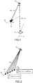
- the figure 3 represents possible steps of the passive locating method according to the invention in the case where it is implemented by at least two receiving stations 10. As seen previously, it is assumed that each receiving station 10 includes a time reference and that all Time references are synchronized with each other.
- the method comprises a first step Etp1 for receiving the pulses and measuring the arrival times of each pulse of the transmitter 15 by each of the receiving stations 10.
- the average arrival time of the pulses at the receiving stations 10 is then calculated by each receiving station during a step Etp2. During this step, each receiving station compresses the received pulses by calculating the average of the arrival times.
- each average time calculated by each receiving station 10 is transmitted to a predetermined receiving station.
- This predetermined station will be responsible for estimating the position of the transmitter from the average times transmitted during an Etp4 calculation step using the Bancroft method and the maximum likelihood method.
- each receiving station 10 other than said predetermined receiving station 10, transmits not each of the arrival times of the received pulses (t np ) but the mean arrival times ( p ). This reduces the data rate between receiving station and therefore allows greater discretion.
- the figure 4 illustrates the geometric configuration associated with the results presented.
- a non-mobile transmitter and a group of P receiving stations 10. It is assumed that the receiving stations 10 are uniformly distributed on a basis of 10 km x 10 km. Of course this example is in no way limiting and the various stations 10 may be distributed in a non-uniform manner.
- D is the distance between the center of this base and the emitter 15.
- Tables 1 and 2 present the standard errors of error on the coordinates [xy ] of the position of the transmitter for a number of pulses N respectively equal to 30 and 3.
- E-TOA The performances of the method according to the invention (denoted E-TOA) are compared with those (denoted E-TDOA) of a standard likelihood maximum TDOA-type estimator for different numbers of receiver stations P and different base-transmitter distances D .
- the figure 5 illustrates examples of ellipses at 90% confidence obtained using the method according to the invention denoted E-TOA, with the aid of an estimator using the method of the maximum likelihood known as E-TDOA and with the Bancroft method noted E-BAN.
- E-TOA 8 receiver stations
- N 10 pulses
- D 200 km.
- the center of the base containing the receiving stations is located in (0, 0).
- Tables 1 and 2 and the figure 5 highlight the best location accuracy of the method according to the invention compared to conventional methods.
Description
La présente invention concerne le domaine de l'écoute électromagnétique. La présente invention concerne plus particulièrement un procédé de localisation passive d'un émetteur non mobile.The present invention relates to the field of electromagnetic listening. The present invention more particularly relates to a method of passive location of a non-mobile transmitter.
Dans un contexte aéroporté ou spatial, la localisation passive d'émetteur peut être effectuée par différentes méthodes comme par exemple, par des mesures d'angle d'arrivée (ou AOA pour « Angle Of Arrival »), d'évolution de phase sur une grande base (ou LBI pour « Long Base Interferometer » ou LBPDE pour «Long Base Phase Difference Evolution »), de différences de temps d'arrivée (ou TDOA pour « Time Difference Of Arrival ») entre au moins deux porteurs, ou encore par Différence de Temps de Passage de Lobe (ou DTPL).In an airborne or spatial context, the emitter passive location can be performed by various methods such as by measurement of angle of arrival (AOA or for "Angle Of Arrival") phase of evolution on a large base (or LBI for "long base Interferometer" or LBPDE for "long base Phase difference Evolution"), differences in arrival time (or TDOA for "time difference of arrival") between at least two carriers, or by Lobe Shift Time Difference (or DTPL).
Les mesures d'angle d'arrivée sont couramment utilisées pour la localisation passive d'émetteurs. Elles nécessitent que les récepteurs soient équipés soit d'un goniomètre d'amplitude, soit d'un interféromètre. Le défaut principal de la localisation par mesure d'angle d'arrivée est son manque de précision quand le temps alloué à la localisation est court.Angle of arrival measurements are commonly used for passive location of transmitters. They require that the receivers are equipped with either an amplitude goniometer or an interferometer. The main defect of location by angle of arrival measurement is its lack of precision when the time allocated to the location is short.
Si l'on dispose d'un interféromètre sur grande base, on peut utiliser des mesures de LBPDE cependant, ces mesures sont sujettes à des ambigüités. De plus, les techniques actuelles de localisation par évolution de phase sur une grande base ou par différence de temps d'arrivée, ne prennent pas en compte le caractère périodique des formes d'onde radar les plus fréquemment rencontrées. Il en résulte, pour ces formes d'ondes, des performances sous-optimales aussi bien en termes de précision de localisation qu'en termes de charge de calcul et d'utilisation de la bande passante entre les porteurs.If a large base interferometer is available, LBPDE measurements can be used, however, these measurements are subject to ambiguities. In addition, current phase-based localization techniques based on a large base or a difference in arrival time do not take into account the periodic nature of the most frequently encountered radar waveforms. As a result, for these waveforms suboptimal performance is achieved both in terms of location accuracy and in terms of computing load and bandwidth utilization between carriers.
Il est connu de l'art antérieur, notament par "
Un problème avec la localisation passive d'émetteurs à l'aide des temps d'arrivée des impulsions (ou TOA pour « Time Of Arrival » ) vient du nombre de mesures à traiter. Lors de l'interception d'un signal, une mesure de TOA est associée à chaque impulsion reçue. Le nombre d'impulsions interceptées, donc de mesures de temps d'arrivée d'impulsions, devient rapidement très grand car ces impulsions sont émises à une cadence très élevée. De plus, avec les solutions existantes, calculer une localisation à partir des TOA implique d'estimer le temps d'arrivée de chaque impulsion.A problem with the passive location of transmitters using pulse arrival times (or TOA for " Time Of Arrival " ) comes from the number of measurements to be processed. When intercepting a signal, a measurement of TOA is associated with each received pulse. The number of impulses intercepted, therefore of pulse arrival time measurements, quickly becomes very large because these pulses are transmitted at a very high rate. In addition, with existing solutions, calculating a location from the TOA involves estimating the arrival time of each pulse.
La complexité du problème d'estimation va donc croitre rapidement avec le nombre d'impulsions. Par exemple, pour un algorithme explicite basé sur la méthode des moindres carrés linéaires, la complexité asymptotique est donnée par 0(I2M) avec I le nombre de paramètres inconnus à estimer et M le nombre de mesures. Dans le cas d'estimation avec les temps d'arrivée on a M=P (nombre de récepteurs) x N (nombre d'impulsions) et I=3 (dimensions spatiales) +N (nombre de dates d'émission inconnues, soit nombre d'impulsions) soit une complexité asymptotique en 0(N 3 P) qui est prohibitive au vu du nombre d'impulsions susceptibles d'être reçues.The complexity of the estimation problem will therefore increase rapidly with the number of pulses. For example, for an explicit algorithm based on the linear least squares method, the asymptotic complexity is given by 0 ( I 2 M ) with I the number of unknown parameters to estimate and M the number of measurements. In the case of estimation with arrival times we have M = P (number of receivers) x N (number of pulses) and I = 3 (spatial dimensions) + N (number of unknown transmission dates, ie number of pulses) is an asymptotic complexity at 0 (N 3 P ) which is prohibitive in view of the number of pulses that can be received.
Concernant la localisation basée sur les différences de temps d'arrivée des impulsions, comme on calcule une différence entre les mesures, on n'a plus à estimer les dates d'émission de chaque impulsion. Cependant, le calcul de cette différence augmente la variance des mesures de TDOA par rapport à celles de TOA et fait apparaitre des corrélations entre les mesures. La matrice de covariance des mesures de différences de temps d'arrivée des impulsions est : 

L'augmentation des termes diagonaux et l'introduction de termes hors-diagonale dans la matrice de covariance des mesures conduit à une légère dégradation des performances de localisation.The increase of the diagonal terms and the introduction of off-diagonal terms in the covariance matrix of the measures leads to a slight degradation of the localization performances.
De plus, l'élimination du paramètre "date d'émission " correspondant à la date de début d'émission des impulsions, enlève la possibilité d'introduire une connaissance a priori sur ce paramètre. Or un a priori permet d'introduire de l'information supplémentaire dans l'estimateur ce qui permet d'améliorer les performances de la localisation finale.In addition, the elimination of the "date of issue" parameter corresponding to the start date of transmission of the pulses, removes the possibility of introducing knowledge a priori on this parameter. However, a priori makes it possible to introduce additional information into the estimator, which improves the performance of the final location.
Un autre problème de la localisation passive par TOA ou TDOA est lié aux communications entre les plateformes. L'une ou l'autre des deux méthodes précédentes implique une communication entre les plateformes pour calculer les résultats de la localisation. Les informations transmises d'une plateforme vers l'autre sont les temps d'arrivée des impulsions reçues. Comme le nombre d'impulsions reçues est important et que les temps d'arrivée doivent être transmis précisément (codés sur un nombre de bits importants), on a donc une forte contrainte sur le débit de la liaison de données. De plus ces transmissions pénalisent la discrétion des plateformes.Another problem of passive localization by TOA or TDOA is related to communications between the platforms. Either of the above two methods involves communication between the platforms to calculate the results of the location. The information transmitted from one platform to the other are the arrival times of the received pulses. Since the number of pulses received is important and the arrival times must be accurately transmitted (coded over a large number of bits), there is therefore a strong constraint on the data link bit rate. Moreover these transmissions penalize the discretion of the platforms.
Un document
Un but de l'invention est notamment de corriger tout ou partie des inconvénients de l'art antérieur en proposant une solution permettant d'améliorer la précision de localisation d'un émetteur non mobile sans pénaliser la discrétion des détecteurs.An object of the invention is in particular to correct all or part of the disadvantages of the prior art by proposing a solution for improving the location accuracy of a non-mobile transmitter without penalizing the discretion of the detectors.
A cet effet, l'invention a pour objet un procédé de localisation passive d'un émetteur non mobile au sol mis en oeuvre par un groupe d'au moins deux stations réceptrices, chacune des stations réceptrices comprenant un détecteur de radars et une référence de temps, l'ensemble des références de temps étant synchronisées entre elles et ledit émetteur émettant un ensemble d'impulsions périodiques, la durée d'un train d'impulsions étant suffisamment courte pour que chacune des stations réceptrices ait toujours une trajectoire assimilable à un mouvement rectiligne uniforme, chaque station réceptrice étant configurée pour mesurer des temps d'arrivés des impulsions de l'émetteur et calculer un temps moyen d'arrivée desdites impulsions, ledit procédé étant caractérisé en ce qu'une première estimation de la position dudit émetteur est réalisée par la méthode de Bancroft à partir des temps moyens d'arrivée des impulsions émise par l'émetteur au niveau de chaque station du groupe d'au moins deux stations réceptrices, le résultat obtenu étant ensuite utilisé comme point d'initialisation d'une méthode de maximum de vraisemblance afin de converger vers la position dudit émetteur.For this purpose, the subject of the invention is a method of passive location of a non-mobile ground transmitter implemented by a group of at least two receiving stations, each of the receiving stations comprising a radar detector and a reference of time, the set of time references being synchronized with each other and said transmitter emitting a set of periodic pulses, the duration of a pulse train being short enough so that each of the receiving stations always has a trajectory similar to a movement uniform rectilinear, each receiving station being configured to measure arrival times pulses of the transmitter and calculate a mean time of arrival of said pulses, said method being characterized in that a first estimate of the position of said transmitter is performed by the Bancroft method from the average arrival times of the pulses emitted by the transmitter at the level of station of the group of at least two receiving stations, the result obtained then being used as the initialization point of a maximum likelihood method in order to converge towards the position of said transmitter.
Selon une variante de mise en oeuvre, le procédé est mis en oeuvre par au moins deux stations réceptrices et ledit procédé comprend :
- Une étape Etp1 de mesure des temps d'arrivés des impulsions de l'émetteur par chaque station réceptrice,
- Une étape Etp2 de calcul du temps moyen d'arrivée des impulsions par chaque station réceptrice,
- Une étape Etp3 de transmission des temps moyens d'arrivée des impulsions calculés à une station réceptrice prédéterminée,
- Une étape Etp4 de calcul, par ladite station réceptrice prédéterminée, de la localisation de l'émetteur à partir de tous les temps moyens d'arrivée des impulsions à l'aide de la méthode de Bancroft puis de la méthode du maximum de vraisemblance.
- A step Etp1 for measuring the arrival times of the pulses of the transmitter by each receiving station,
- An Etp2 step of calculating the average arrival time of the pulses by each receiving station,
- A step Etp3 transmitting the average arrival times of the pulses calculated at a predetermined receiving station,
- An Etp4 step of calculating, by said predetermined receiving station, the location of the transmitter from all mean arrival times of the pulses using the Bancroft method and then the maximum likelihood method.
Selon une variante de mise en oeuvre, la ou les stations réceptrices sont sont des stations réceptrices aéroportées.According to an alternative embodiment, the receiving station or stations are airborne receiving stations.
Selon une variante de mise en oeuvre, la ou les stations réceptrices sont des stations réceptrices spatiales.According to an implementation variant, the receiving station or stations are spatial receiver stations.
Les avantages fournis, outre l'optimalité de l'estimation dans les cas des émetteurs périodiques, sont relatifs à la quantité restreinte de données échangées entre les stations réceptrices ainsi qu'à la précision de localisation atteignable en un temps aussi court qu'un train d'impulsions radar. Par ailleurs un avantage important apporté par l'invention est une initialisation pertinente des algorithmes itératifs d'estimation de la position à partir des mesures de temps d'arrivée.The advantages provided, besides the optimality of the estimation in the case of periodic transmitters, relate to the limited amount of data exchanged between the receiving stations as well as to the location accuracy achievable in a time as short as a train. radar pulses. Furthermore, an important advantage provided by the invention is a relevant initialization of the iterative algorithms for estimating the position from the arrival time measurements.
D'autres particularités et avantages de la présente invention apparaîtront plus clairement à la lecture de la description ci-après, donnée à titre illustratif et non limitatif, et faite en référence aux dessins annexés, dans lesquels :
- La
figure 1 illustre un exemple de mise en oeuvre du procédé de localisation selon l'invention ; - La
figure 2 représente les temps d'arrivées d'impulsions au niveau d'une station réceptrice à différents instants ; - La
figure 3 illustre des étapes possibles du procédé de localisation selon l'invention ; - La
figure 4 représente la configuration utilisée pour les résultats présentés ; - La
figure 5 représente des exemples d'ellipses à 90% de confiance obtenues à l'aide du procédé selon l'invention.
- The
figure 1 illustrates an example of implementation of the localization method according to the invention; - The
figure 2 represents the arrival times of pulses at a receiving station at different times; - The
figure 3 illustrates possible steps of the locating method according to the invention; - The
figure 4 represents the configuration used for the results presented; - The
figure 5 represents examples of ellipses at 90% confidence obtained using the method according to the invention.
Le principe de la localisation passive selon l'invention repose sur une estimation de la position d'un émetteur non mobile au sol en deux temps à l'aide de deux méthodes de calcul différentes.The principle of passive location according to the invention is based on an estimate of the position of a non-mobile transmitter on the ground in two stages using two different calculation methods.
Classiquement, le calcul de la position d'un émetteur est effectué à l'aide d'une estimation du maximum de vraisemblance. Le problème est que cette méthode est difficile à appliquer directement car elle implique des équations non linéaires compliquées à résoudre. L'estimateur maximise une fonction qui comporte plusieurs maxima locaux. De plus, cet algorithme est très sensible aux conditions initiales et a besoin d'avoir une bonne initialisationpour converger vers le maximum global de vraisemblance.Conventionally, the calculation of the position of an issuer is performed using a maximum likelihood estimate. The problem is that this method is difficult to apply directly because it involves complicated nonlinear equations to solve. The estimator maximizes a function that has several local maxima. In addition, this algorithm is very sensitive to initial conditions and needs to have good initialization to converge towards the global maximum of likelihood.
L'invention propose d'effectuer en deux temps l'optimisation du critère de maximum de vraisemblance. Une première estimation sommaire est faite avec la méthode de Bancroft connue de l'homme du métier notamment par "
L'utilisation d'une première estimation sommaire a pour avantage de fournir un point d'initialisation, pour l'algorithme de maximum de vraisemblance, qui est suffisamment proche de la solution pour converger vers le maximum global et non vers un maximum local. De plus, cela permet de réduire le nombre d'itérations de l'algorithme de maximum de vraisemblance.The use of a first summary estimate has the advantage of providing an initialization point, for the maximum likelihood algorithm, which is sufficiently close to the solution to converge towards the global maximum and not towards a local maximum. In addition, this reduces the number of iterations of the maximum likelihood algorithm.
En référence aux
On suppose que l'émetteur 15 émet un train de N impulsions périodiques (N représentant un entier strictement positif) avec une période de récurrence notée T. Dans ces conditions, le temps d'émission de la nième impulsion peut s'écrire : ![]()
![]()
![]()
![]()
Le temps d'arrivée tn,p de l'impulsion d'indice n sur la pième station réceptrice (avec p=1,...,P) est le temps d'émission de l'impulsion ajouté au temps de propagation vers la station, avec un bruit de mesure. Ce temps d'arrivée peut s'écrire : ![]()
- Où : c représente la vitesse de propagation,
- rp(tn,p) représente la distance entre l'émetteur et la pième station réceptrice au temps d'arrivée tn,p
- t0 représente le temps d'émission de l'impulsion,
- T représente la période de répétition des impulsions
- wn,p représente le bruit de mesure supposé gaussien, centré et indépendant en n (d'une mesure à l'autre) et en p (d'un récepteur à l'autre) de variance
notée 
- Where: c represents the speed of propagation,
- r p (t n, p ) represents the distance between the transmitter and the p th receiving station at the arrival time t n, p
- t 0 represents the emission time of the pulse,
- T represents the repetition period of the pulses
- w n, p represents the measurement noise assumed Gaussian, centered and independent in n (from one measurement to another) and in p (from one receiver to another) of variance noted
On suppose que la durée d'un train d'impulsions est suffisamment courte pour que chacune des P stations réceptrices ait toujours une trajectoire 12 assimilable à un mouvement rectiligne uniforme. Sous ces hypothèses on peut vérifier que : ![]()
![]()
- r0,p représente la distance entre l'émetteur et la pième station réceptrice au milieu de sa trajectoire,
- T représente la période de récurrence ou période de répétition des impulsions ;
- wn,p représente le bruit lié à la nième impulsion sur la pième station réceptrice.
- r 0, p represents the distance between the transmitter and the p th receiving station in the middle of its trajectory,
- T represents the recurrence period or repetition period of the pulses;
- w n, p represents the noise related to the n th pulse on the p th receiver station.
Le modèle (2) va permettre d'estimer la période de récurrence des impulsions T et le temps moyen d'arrivée des impulsions sur la station réceptrice d'indice p, p variant de 1 à P.The model (2) will make it possible to estimate the recurrence period of the pulses T and the mean arrival time of the pulses on the receiving station with index p, p varying from 1 to P.
La relation non linéaire entre (ap)p=1...P et les coordonnées de l'émetteur, implicites dans r0,p, pourra ensuite être inversée par un algorithme explicite ce qui fournira une initialisation pertinente des algorithmes itératifs d'estimation fine de la position de la cible.The nonlinear relation between (a p ) p = 1 ... P and the emitter coordinates, implied in r 0, p , can then be inverted by an explicit algorithm which will provide a relevant initialization of the iterative algorithms of Fine estimate of the position of the target.
On considère le cas particulier de la localisation passive d'un émetteur 15 par une seule station réceptrice 10. Si P=1 on peut mettre les équations (2) sous la forme vectorielle suivante : ![]()

![]()
Les vecteurs τ1, θ 1 et w 1, sont de taille N et la matrice H1 est de taille Nx2. Les composantes du bruit w1 étant Gaussiennes, centrées et indépendantes, l'estimation du maximum de vraisemblance pour les paramètres θ 1 est donnée par la résolution du problème des moindres carrés dont la solution est classiquement donnée par : ![]()
![]()


![]()
![]()
Où â 1 représente l'estimation du temps moyen d'arrivée des impulsions sur la station réceptrice et l'émetteur et T̂ représente l'estimation de la période de récurence.Where ? 1 represents the estimate of the average arrival time of the pulses on the receiving station and the transmitter and T represents the estimation of the recursion period.
On considère maintenant le cas d'un nombre de stations réceptrices 10 au moins égal à 2.We now consider the case of a number of receiving
Si P>1, on peut mettre les équations (2) sous une forme vectorielle similaire à l'équation (3) précédente de la manière suivante : ![]()


![]()
Les vecteurs τP, θP et wP sont de taille NP et la matrice HP est de taille NPx(P+1). De même que dans le cas précédent où P=1, les composantes du bruit wP sont Gaussiennes, centrées et indépendantes. Si leur variance est la même pour toutes les stations, l'estimation du maximum de vraisemblance pour les paramètres θ p est encore donnée par la résolution du problème des moindres carrés dont la solution est : ![]()


![]()
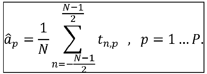
Où âp représente l'estimation du temps moyen d'arrivée des impulsions sur la station réceptrice d'indice p et l'émetteur et T̂ représente l'estimation de la période de récurrence des impulsions.Where p represents the estimate of the average arrival time of the pulses on the receiving station of index p and the transmitter and T represents the estimate of the period of recurrence of the pulses.
Les expressions obtenues montrent que le procédé d'estimation peut être mis en oeuvre en calculant le temps moyen d'arrivée sur chacune des stations puis en mettant en commun les résultats obtenus pour en déduire une estimation de la position de la cible.The expressions obtained show that the estimation method can be implemented by calculating the mean arrival time on each of the stations and then pooling the results obtained to derive an estimate of the position of the target.
L'estimation de la période de récurrence est donnée quant à elle par la moyenne des P estimations faites individuellement par chaque station.The estimate of the recurrence period is given by the average of the estimates made individually by each station.
Si la variance du bruit n'est pas la même d'une station à l'autre, l'estimation de θ p est modifiée en la résolution du problème des moindres carrés pondérés, ce qui ne change que l'expression finale de T̂ où la moyenne devient une moyenne pondérée, mais pas celles de â p, p =1...P.If the variance of the noise is not the same from one station to another, the estimation of θ p is modified in the resolution of the weighted least squares problem, which only changes the final expression of T where the average becomes a weighted average, but not those of â p , p = 1 ... P.
Comme vu précédemment, l'estimation de la position de l'émetteur est réalisée en deux temps. Une première estimation grossière est calculée par la méthode de Bancroft. Le résultat obtenu est ensuite utilisée comme point d'initialisation pour une méthode du maximum de vraisemblance (également connue sous le sigle anglo saxon MLE pour " Maximum Likelihood Estimator ").As seen above, the estimation of the position of the transmitter is carried out in two stages. A rough first estimate is calculated by the Bancroft method. The result obtained is then used as an initialization point for a maximum likelihood method (also known as MLE for the "Maximum Likelihood Estimator").
Les expressions de âp obtenues précédemment correspondent à des réalisations de variables aléatoires de moyenne ![]()
![]()
![]()
![]()
La relation entre r0p, la position (x,y,z) de l'émetteur, et la position (xp,yp,zp) de la pième station est : ![]()
![]()
![]()
![]()
En élevant les deux expressions de r0p au carré, on obtient pour tout p=1...P : 
Cette dernière expression fait apparaître la fonctionnelle de Minkowski notée <.|.> telle que pour tous vecteurs de dimension quatre v=(v1,v2,v3,v4) et w=(w1,w2,w3,w4) on ait : ![]()
![]()
Si on place les informations liées à une station réceptrice p dans un vecteur sp et les inconnues dans un vecteur u : 


![]()
![]()
Le système ci-dessus est sur-dimensionné pour un nombre de stations réceptrices supérieur à 4 (P équations pour 4 inconnues). Ce système peut être résolu avec la pseudo-inverse B+ de la matrice B en supposant Λ connu dans un premier temps : ![]()
![]()
![]()
![]()
En utilisant cette dernière expression de u pour développer l'expression de Λ=<u|u>, on obtient un trinôme du second degré en Λ : ![]()
![]()
Ce dernier fournit deux solutions candidates pour Λ, notées Λ1 et Λ2, conduisant à deux solutions possibles u1 et u2 au problème : ![]()
![]()
Une de ces deux solutions sera cohérente par rapport à la situation. Par exemple, l'altitude estimée sera proche de la surface de la terre.One of these two solutions will be consistent with the situation. For example, the estimated altitude will be close to the surface of the earth.
Comme vu précédemment, la position trouvée par la méthode de Bancroft est ensuite utilisée comme point d'initialisation pour une estimation du maximum de vraisemblance.As seen previously, the position found by the Bancroft method is then used as the initialization point for a maximum likelihood estimate.
Dans cette deuxième estimation, On prend maintenant en compte le bruit wn dans les mesures de temps d'arrivée des impulsions. L'expression des ![]()
![]()
- Où : c représente la vitesse de propagation des impulsions,
- (x, y, z) représente les coordonnées de la position de l'émetteur,
- (xp, yp, zp) représente les coordonnées de la position de la pième station réceptrice,
- t0 représente la date de début d'émission des impulsions,
- fp représente une fonction non linéaire qui relie la position de l'émetteur et la date de début d'émission. Cette fonction fp représente le temps d'arrivée de l'impulsion sans bruit au niveau de la pieme station,
- wn représente le bruit de mesure considéré comme un bruit gaussien de variance

avec 
- Where: c represents the speed of propagation of the pulses,
- (x, y, z) represents the coordinates of the position of the transmitter,
- (x p , y p , z p ) represents the coordinates of the position of the p th receiving station,
- t 0 represents the start date of transmission of the pulses,
- f p represents a non-linear function that links the position of the transmitter and the start date of transmission. This function f p represents the arrival time of the impulse without noise at the p th station,
- w n represents the measurement noise considered as a Gaussian noise of variance
Suivant un mode de mise en oeuvre de l'invention la méthode du maximum de vraisemblance peut contenir un a priori sur le paramètre t 0 correspondant à la date d'émission de l'impulsion au centre du train d'impulsions émis par l'émetteur. On peut considérer, sans perte de généralité, que les impulsions sont datées en prenant comme origine la date de réception de l'impulsion centrale par la première station réceptrice (10) : ![]()
![]()
Ainsi si l'on considère que les distances émetteur-stations réceptrices sont très supérieures aux distances entre les stations réceptrices (cas des bases courtes : par exemple la distance entre l'émetteur et la stations peut être de l'ordre de 200 km alors que la distance entre les stations peut être de l'ordre du km), on peut considérer que la distance ![]()
![]()
![]()
![]()
![]()
![]()
On choisit ![]()
![]()
En pratique, même si l'émetteur est très proche des stations réceptrices, cet a priori n'introduit quasiment pas de biais car l'information qu'il apporte devient de plus en plus négligeable comparée à l'information apportée par les mesures réelles au fur et à mesure que l'émetteur se rapproche.In practice, even if the transmitter is very close to the receiving stations, this a priori introduces almost no bias because the information it provides becomes more and more negligible compared to the information provided by the actual measurements. as the transmitter gets closer.
Pour les P stations réceptrices on a le vecteur de mesures suivant : 
La matrice de covariance liée à ces mesures (supposées indépendantes) est: 
Si on fait une approximation linéaire au point ( x i , y i, z i, t 0 i ) pour les fonctions f p on obtient : 


Cette variable matricielle ε représente l'erreur d'approximation à l'itération courante. La première colonne représente l'erreur d'approximation en x, la deuxième en y, la troisième en z et la dernière en t0.This matrix variable ε represents the approximation error at the current iteration. The first column represents the approximation error in x, the second in y, the third in z and the last in t 0 .
On minimise le critère c défini par : ![]()
![]()
Cela revient à minimiser la norme du vecteur d'erreur pondéré par la matrice ∑ qui contient les variances des estimateurs ![]()
![]()
On obtient donc une nouvelle estimation de la position avec : ![]()
![]()
On réitère la procédure jusqu'à ce que Δ, le vecteur de déplacement vers la nouvelle position, soit inférieur à un seuil prédéterminé. Suivant un mode de mis en oeuvre, on peut choisir comme contrainte, par exemple, ∥Δ∥ < 1 m.The procedure is repeated until Δ, the displacement vector to the new position, is less than a predetermined threshold. According to one mode of implementation, one can choose as constraint, for example, ∥Δ∥ <1 m .
La
Le procédé comprend une première étape Etp1 de réception des impulsions et de mesure des temps d'arrivés de chaque impulsion de l'émetteur 15 par chacune des stations réceptrices 10.The method comprises a first step Etp1 for receiving the pulses and measuring the arrival times of each pulse of the
Le temps moyen d'arrivée des impulsions au niveau des stations réceptrices 10 est ensuite calculé par chaque station réceptrice au cours d'une étape Etp2. Lors de cette étape, chaque station réceptrice effectue une compression des impulsions reçues en calculant la moyenne des temps d'arrivée.The average arrival time of the pulses at the receiving
Au cours d'une étape Etp3 de transmission, chaque temps moyen calculé par chaque station réceptrice 10 est transmis à une station réceptrice prédéterminée. Cette station prédéterminée sera chargée d'estimer la position de l'émetteur à partir des temps moyens transmis au cours d'une étape de calcul Etp4 à l'aide de la méthode de Bancroft puis de la méthode du maximum de vraisemblance.During a transmission step Etp3, each average time calculated by each receiving
De façon avantageuse, chaque station réceptrice 10, autre que ladite station réceptrice 10 prédéterminée, transmet non pas chacun des temps d'arrivée des impulsions reçues (tnp) mais les temps moyens d'arrivée (âp ). Ceci permet de réduire le débit de données entre station réceptrice et donc permet une plus grande discrétion.Advantageously, each receiving
Les tableaux 1 et 2 ci-dessous, illustrent des exemples de résultats obtenus en appliquant le procédé selon l'invention.Tables 1 and 2 below illustrate examples of results obtained by applying the method according to the invention.
La
Dans ces mesures, les paramètres fixés sont :
- σTOA = 30 ns : bruit de mesure du TOA sur chaque récepteur,
-

- σ d
0 = 50 km : écart-type de l'a priori, - Problème ramené à deux dimensions.
- σ TOA = 30 ns: measurement noise of the TOA on each receiver,
-
- σ d
0 = 50 km: standard deviation of the prior, - Problem reduced to two dimensions.
Les tableaux 1 et 2 présentent les écarts types d'erreur sur les coordonnées [x y] de la position de l'émetteur pour un nombre d'impulsions N respectivement égal à 30 et 3.Tables 1 and 2 present the standard errors of error on the coordinates [xy ] of the position of the transmitter for a number of pulses N respectively equal to 30 and 3.
Les performances du procédé selon l'invention (notées E-TOA) sont comparées avec celles (notées E-TDOA) d'un estimateur du type TDOA par maximum de vraisemblance classique pour différents nombres de stations réceptrices P et différentes distances base-émetteur D.
La
Les tableaux 1 et 2 ainsi que la
Comme vu précédemment, le fait de transmettre les temps moyen d'arrivée des impulsions plutôt que toutes les impulsions reçues permet de réduire la quantité de données échangées entre les stations réceptrices et permet donc une plus grande discrétion des stations.As seen previously, the fact of transmitting the average arrival times of the pulses rather than all the pulses received makes it possible to reduce the amount of data exchanged between the receiving stations and thus allows a greater discretion of the stations.
Le tableau ci-dessous présente le nombre de transfert de données entre deux stations réceptrices pour N=3 et N=100 impulsions dans le cas du procédé selon l'invention (E-TOA) et celui d'un estimateur utilisant la méthode du maximum de vraisemblance classique (E-TDOA).
Claims (4)
- A method for passively locating a non-movable transmitter (15) on the ground implemented by a group of at least two receiving stations (10), each of the receiving stations (10) comprising a detector of radars and a time reference, the set of time references being mutually synchronized, said transmitter (15) transmitting a set of periodic pulses, the duration of a pulse train being sufficiently short for each of the receiving stations (10) to always have a trajectory (12) that can be regarded as a uniform rectilinear motion, each receiving station (10) being configured to measure arrival times of the pulses of the transmitter (15) and to compute a mean arrival time of said pulses, said method being characterized in that a first estimation of the position of said transmitter (15) is carried out by the Bancroft scheme on the basis of the mean arrival times of the pulses transmitted by the transmitter (15) at the level of each station (10) of the group of at least two receiving stations (10),
the result obtained being used thereafter as point for initializing a maximum likelihood scheme so as to converge toward the position of said transmitter. - The method as claimed in the preceding claim, implemented by at least two receiving stations (10) in which said method comprises:- A step Etp1 of measuring the arrival times of the pulses of the transmitter (15) by each receiving station (10),- A step Etp2 of computing the mean arrival time of the pulses by each receiving station (10),- A step Etp3 of dispatching the computed mean arrival times of the pulses to a predetermined receiving station (10),- A step Etp4 of computing, by said predetermined receiving station (10), the location of the transmitter (15) on the basis of all the mean arrival times of the pulses with the aid of the Bancroft scheme and then of the maximum likelihood scheme.
- The method as claimed in one of the preceding claims, in which the receiving station or stations (10) are airborne receiving stations.
- The method as claimed in one of claims 1 or 2, in which the receiving station or stations (10) are space receiving stations.
Applications Claiming Priority (2)
| Application Number | Priority Date | Filing Date | Title |
|---|---|---|---|
| FR1402710A FR3029300A1 (en) | 2014-11-28 | 2014-11-28 | PASSIVE LOCATION METHOD OF NON-MOBILE TRANSMITTER |
| PCT/EP2015/076227 WO2016083124A1 (en) | 2014-11-28 | 2015-11-10 | Method for passively locating a non-movable transmitter |
Publications (2)
| Publication Number | Publication Date |
|---|---|
| EP3234629A1 EP3234629A1 (en) | 2017-10-25 |
| EP3234629B1 true EP3234629B1 (en) | 2018-12-26 |
Family
ID=53008560
Family Applications (1)
| Application Number | Title | Priority Date | Filing Date |
|---|---|---|---|
| EP15801131.2A Active EP3234629B1 (en) | 2014-11-28 | 2015-11-10 | Method for passively locating a non-movable transmitter |
Country Status (4)
| Country | Link |
|---|---|
| US (1) | US10156630B2 (en) |
| EP (1) | EP3234629B1 (en) |
| FR (1) | FR3029300A1 (en) |
| WO (1) | WO2016083124A1 (en) |
Families Citing this family (2)
| Publication number | Priority date | Publication date | Assignee | Title |
|---|---|---|---|---|
| FR3104735B1 (en) | 2019-12-11 | 2021-11-12 | Thales Sa | PROCESS FOR PASSIVE LOCATION OF TRANSMITTERS BY MEASURING DIFFERENTIAL TIME OF ARRIVAL (TDOA) |
| CN115825863B (en) * | 2022-12-16 | 2023-12-29 | 南京航空航天大学 | Method for rapidly and directly positioning non-circular signal under impact noise |
Family Cites Families (10)
| Publication number | Priority date | Publication date | Assignee | Title |
|---|---|---|---|---|
| US5740048A (en) * | 1992-08-07 | 1998-04-14 | Abel; Jonathan S. | Method and apparatus for GPS positioning, filtering and integration |
| US6330452B1 (en) * | 1998-08-06 | 2001-12-11 | Cell-Loc Inc. | Network-based wireless location system to position AMPs (FDMA) cellular telephones, part I |
| US7132982B2 (en) * | 1999-03-05 | 2006-11-07 | Rannock Corporation | Method and apparatus for accurate aircraft and vehicle tracking |
| US6408246B1 (en) * | 2000-10-18 | 2002-06-18 | Xircom Wireless, Inc. | Remote terminal location algorithm |
| US20050175038A1 (en) * | 2004-01-12 | 2005-08-11 | John Carlson | Method and apparatus for synchronizing wireless location servers |
| DE102008032983A1 (en) * | 2008-07-08 | 2010-02-25 | Fraunhofer-Gesellschaft zur Förderung der angewandten Forschung e.V. | Method and device for determining the changing position of a mobile transmitter |
| US7453400B2 (en) * | 2007-02-02 | 2008-11-18 | Bae Systems Information And Electronic Systems Integration Inc. | Multiplatform TDOA correlation interferometer geolocation |
| CH699326A1 (en) * | 2008-08-13 | 2010-02-15 | Thales Suisse Sa | Transmitter i.e. airplane, position determining time difference of arrival method for military application, involves outputting calculated transmitter positions when results of physical consistency check is positive |
| ES2615269T3 (en) * | 2012-02-21 | 2017-06-06 | Karlsruher Institut für Technologie | Procedure and system of calibration of receivers and location of simultaneous objects for multilateration |
| FR3000223B1 (en) * | 2012-12-21 | 2020-01-10 | Thales | METHOD AND PASSIVE ENUMERATION AND / OR LOCATION OF RADAR TRANSMITTERS AND ASSOCIATED SYSTEM |
-
2014
- 2014-11-28 FR FR1402710A patent/FR3029300A1/en active Pending
-
2015
- 2015-11-10 US US15/526,751 patent/US10156630B2/en active Active
- 2015-11-10 EP EP15801131.2A patent/EP3234629B1/en active Active
- 2015-11-10 WO PCT/EP2015/076227 patent/WO2016083124A1/en active Application Filing
Non-Patent Citations (1)
| Title |
|---|
| None * |
Also Published As
| Publication number | Publication date |
|---|---|
| EP3234629A1 (en) | 2017-10-25 |
| WO2016083124A1 (en) | 2016-06-02 |
| FR3029300A1 (en) | 2016-06-03 |
| US10156630B2 (en) | 2018-12-18 |
| US20170336492A1 (en) | 2017-11-23 |
Similar Documents
| Publication | Publication Date | Title |
|---|---|---|
| US9407317B2 (en) | Differential ultra-wideband indoor positioning method | |
| CN107678050B (en) | GLONASS phase inter-frequency deviation real-time tracking and precise estimation method based on particle filtering | |
| EP2469361B1 (en) | Method for underwater time service and synchronization and system thereof | |
| EP1712930B1 (en) | System and procedure for determining the instantaneous speed of an object | |
| CN104199280B (en) | A kind of time synchronization error measuring method based on differential GPS | |
| EP2929364B1 (en) | Method for the passive localization of radar transmitters | |
| EP2626723B1 (en) | Method for estimating the incoming direction of navigation signals in a receiver after reflecting off walls in a satellite positioning system | |
| KR20010098736A (en) | Obtaining pilot phase offset time delay parameter for a wireless terminal of an integrated wireless-global positioning system | |
| EP2410352A1 (en) | Antenna device with synthetic opening for receiving signals of a system including a carrier and a means for determining the trajectory thereof | |
| FR2979710A1 (en) | ACOUSTIC POSITIONING DEVICE AND METHOD | |
| CN111149018A (en) | Method and system for calibrating system parameters | |
| Wann et al. | NLOS mitigation with biased Kalman filters for range estimation in UWB systems | |
| EP3234629B1 (en) | Method for passively locating a non-movable transmitter | |
| EP3391072B1 (en) | Method for locating sources emitting electromagnetic pulses | |
| FR2801682A1 (en) | Satellite telecommunications parasitic transmission position location technique having interferometric frequency difference measurement providing detection satellite/line parasitic transmitter/satellite angle | |
| KR100899545B1 (en) | All-in-view time transfer by use of code and carrier phase measurements of GNSS satellites | |
| CA2901647C (en) | Sonar device and process for determining displacement speed of a naval vehicle on the sea bed | |
| FR3070515A1 (en) | METHOD FOR DETERMINING THE TRACK OF A MOBILE OBJECT, PROGRAM AND DEVICE SUITABLE FOR THE IMPLEMENTATION OF SAID METHOD | |
| EP4073536B1 (en) | Method for passively locating transmitters by means of time difference of arrival (tdoa) | |
| FR2874095A1 (en) | METHOD FOR ANGULAR CALIBRATION OF AN ANTENNA BY MEASURING THE RELATIVE DISTANCE | |
| EP2626725B1 (en) | Method for determining a confidence indicator relating to the path taken by a mobile | |
| EP3492943A1 (en) | Method and system for position estimation by collaborative repositioning using landmarks with imprecise positions | |
| FR3003961A1 (en) | METHOD FOR SIGNAL BEAM FORMATION OF A SIGNAL RECEIVER OF A SATELLITE NAVIGATION SYSTEM FOR IMPROVING INTERFERENCE RESISTANCE. | |
| EP4361661A1 (en) | Method for precisely time broadcasting by fuzzy position beacon network | |
| EP2439556B1 (en) | Method for identifying emitters by a terminal in an iso-frequency network |
Legal Events
| Date | Code | Title | Description |
|---|---|---|---|
| STAA | Information on the status of an ep patent application or granted ep patent |
Free format text: STATUS: THE INTERNATIONAL PUBLICATION HAS BEEN MADE |
|
| PUAI | Public reference made under article 153(3) epc to a published international application that has entered the european phase |
Free format text: ORIGINAL CODE: 0009012 |
|
| STAA | Information on the status of an ep patent application or granted ep patent |
Free format text: STATUS: REQUEST FOR EXAMINATION WAS MADE |
|
| 17P | Request for examination filed |
Effective date: 20170517 |
|
| AK | Designated contracting states |
Kind code of ref document: A1 Designated state(s): AL AT BE BG CH CY CZ DE DK EE ES FI FR GB GR HR HU IE IS IT LI LT LU LV MC MK MT NL NO PL PT RO RS SE SI SK SM TR |
|
| AX | Request for extension of the european patent |
Extension state: BA ME |
|
| DAV | Request for validation of the european patent (deleted) | ||
| DAX | Request for extension of the european patent (deleted) | ||
| GRAP | Despatch of communication of intention to grant a patent |
Free format text: ORIGINAL CODE: EPIDOSNIGR1 |
|
| STAA | Information on the status of an ep patent application or granted ep patent |
Free format text: STATUS: GRANT OF PATENT IS INTENDED |
|
| INTG | Intention to grant announced |
Effective date: 20181005 |
|
| GRAS | Grant fee paid |
Free format text: ORIGINAL CODE: EPIDOSNIGR3 |
|
| GRAA | (expected) grant |
Free format text: ORIGINAL CODE: 0009210 |
|
| STAA | Information on the status of an ep patent application or granted ep patent |
Free format text: STATUS: THE PATENT HAS BEEN GRANTED |
|
| AK | Designated contracting states |
Kind code of ref document: B1 Designated state(s): AL AT BE BG CH CY CZ DE DK EE ES FI FR GB GR HR HU IE IS IT LI LT LU LV MC MK MT NL NO PL PT RO RS SE SI SK SM TR |
|
| REG | Reference to a national code |
Ref country code: GB Ref legal event code: FG4D Free format text: NOT ENGLISH |
|
| REG | Reference to a national code |
Ref country code: CH Ref legal event code: EP |
|
| REG | Reference to a national code |
Ref country code: AT Ref legal event code: REF Ref document number: 1082169 Country of ref document: AT Kind code of ref document: T Effective date: 20190115 |
|
| REG | Reference to a national code |
Ref country code: DE Ref legal event code: R096 Ref document number: 602015022477 Country of ref document: DE |
|
| REG | Reference to a national code |
Ref country code: IE Ref legal event code: FG4D Free format text: LANGUAGE OF EP DOCUMENT: FRENCH |
|
| PG25 | Lapsed in a contracting state [announced via postgrant information from national office to epo] |
Ref country code: LV Free format text: LAPSE BECAUSE OF FAILURE TO SUBMIT A TRANSLATION OF THE DESCRIPTION OR TO PAY THE FEE WITHIN THE PRESCRIBED TIME-LIMIT Effective date: 20181226 Ref country code: HR Free format text: LAPSE BECAUSE OF FAILURE TO SUBMIT A TRANSLATION OF THE DESCRIPTION OR TO PAY THE FEE WITHIN THE PRESCRIBED TIME-LIMIT Effective date: 20181226 Ref country code: LT Free format text: LAPSE BECAUSE OF FAILURE TO SUBMIT A TRANSLATION OF THE DESCRIPTION OR TO PAY THE FEE WITHIN THE PRESCRIBED TIME-LIMIT Effective date: 20181226 Ref country code: BG Free format text: LAPSE BECAUSE OF FAILURE TO SUBMIT A TRANSLATION OF THE DESCRIPTION OR TO PAY THE FEE WITHIN THE PRESCRIBED TIME-LIMIT Effective date: 20190326 Ref country code: NO Free format text: LAPSE BECAUSE OF FAILURE TO SUBMIT A TRANSLATION OF THE DESCRIPTION OR TO PAY THE FEE WITHIN THE PRESCRIBED TIME-LIMIT Effective date: 20190326 Ref country code: FI Free format text: LAPSE BECAUSE OF FAILURE TO SUBMIT A TRANSLATION OF THE DESCRIPTION OR TO PAY THE FEE WITHIN THE PRESCRIBED TIME-LIMIT Effective date: 20181226 |
|
| REG | Reference to a national code |
Ref country code: NL Ref legal event code: MP Effective date: 20181226 |
|
| REG | Reference to a national code |
Ref country code: LT Ref legal event code: MG4D |
|
| PG25 | Lapsed in a contracting state [announced via postgrant information from national office to epo] |
Ref country code: AL Free format text: LAPSE BECAUSE OF FAILURE TO SUBMIT A TRANSLATION OF THE DESCRIPTION OR TO PAY THE FEE WITHIN THE PRESCRIBED TIME-LIMIT Effective date: 20181226 Ref country code: SE Free format text: LAPSE BECAUSE OF FAILURE TO SUBMIT A TRANSLATION OF THE DESCRIPTION OR TO PAY THE FEE WITHIN THE PRESCRIBED TIME-LIMIT Effective date: 20181226 Ref country code: GR Free format text: LAPSE BECAUSE OF FAILURE TO SUBMIT A TRANSLATION OF THE DESCRIPTION OR TO PAY THE FEE WITHIN THE PRESCRIBED TIME-LIMIT Effective date: 20190327 Ref country code: RS Free format text: LAPSE BECAUSE OF FAILURE TO SUBMIT A TRANSLATION OF THE DESCRIPTION OR TO PAY THE FEE WITHIN THE PRESCRIBED TIME-LIMIT Effective date: 20181226 |
|
| REG | Reference to a national code |
Ref country code: AT Ref legal event code: MK05 Ref document number: 1082169 Country of ref document: AT Kind code of ref document: T Effective date: 20181226 |
|
| PG25 | Lapsed in a contracting state [announced via postgrant information from national office to epo] |
Ref country code: NL Free format text: LAPSE BECAUSE OF FAILURE TO SUBMIT A TRANSLATION OF THE DESCRIPTION OR TO PAY THE FEE WITHIN THE PRESCRIBED TIME-LIMIT Effective date: 20181226 |
|
| PG25 | Lapsed in a contracting state [announced via postgrant information from national office to epo] |
Ref country code: PT Free format text: LAPSE BECAUSE OF FAILURE TO SUBMIT A TRANSLATION OF THE DESCRIPTION OR TO PAY THE FEE WITHIN THE PRESCRIBED TIME-LIMIT Effective date: 20190426 Ref country code: CZ Free format text: LAPSE BECAUSE OF FAILURE TO SUBMIT A TRANSLATION OF THE DESCRIPTION OR TO PAY THE FEE WITHIN THE PRESCRIBED TIME-LIMIT Effective date: 20181226 Ref country code: ES Free format text: LAPSE BECAUSE OF FAILURE TO SUBMIT A TRANSLATION OF THE DESCRIPTION OR TO PAY THE FEE WITHIN THE PRESCRIBED TIME-LIMIT Effective date: 20181226 Ref country code: PL Free format text: LAPSE BECAUSE OF FAILURE TO SUBMIT A TRANSLATION OF THE DESCRIPTION OR TO PAY THE FEE WITHIN THE PRESCRIBED TIME-LIMIT Effective date: 20181226 |
|
| PG25 | Lapsed in a contracting state [announced via postgrant information from national office to epo] |
Ref country code: SM Free format text: LAPSE BECAUSE OF FAILURE TO SUBMIT A TRANSLATION OF THE DESCRIPTION OR TO PAY THE FEE WITHIN THE PRESCRIBED TIME-LIMIT Effective date: 20181226 Ref country code: IS Free format text: LAPSE BECAUSE OF FAILURE TO SUBMIT A TRANSLATION OF THE DESCRIPTION OR TO PAY THE FEE WITHIN THE PRESCRIBED TIME-LIMIT Effective date: 20190426 Ref country code: SK Free format text: LAPSE BECAUSE OF FAILURE TO SUBMIT A TRANSLATION OF THE DESCRIPTION OR TO PAY THE FEE WITHIN THE PRESCRIBED TIME-LIMIT Effective date: 20181226 Ref country code: RO Free format text: LAPSE BECAUSE OF FAILURE TO SUBMIT A TRANSLATION OF THE DESCRIPTION OR TO PAY THE FEE WITHIN THE PRESCRIBED TIME-LIMIT Effective date: 20181226 Ref country code: EE Free format text: LAPSE BECAUSE OF FAILURE TO SUBMIT A TRANSLATION OF THE DESCRIPTION OR TO PAY THE FEE WITHIN THE PRESCRIBED TIME-LIMIT Effective date: 20181226 |
|
| REG | Reference to a national code |
Ref country code: DE Ref legal event code: R097 Ref document number: 602015022477 Country of ref document: DE |
|
| PG25 | Lapsed in a contracting state [announced via postgrant information from national office to epo] |
Ref country code: AT Free format text: LAPSE BECAUSE OF FAILURE TO SUBMIT A TRANSLATION OF THE DESCRIPTION OR TO PAY THE FEE WITHIN THE PRESCRIBED TIME-LIMIT Effective date: 20181226 Ref country code: DK Free format text: LAPSE BECAUSE OF FAILURE TO SUBMIT A TRANSLATION OF THE DESCRIPTION OR TO PAY THE FEE WITHIN THE PRESCRIBED TIME-LIMIT Effective date: 20181226 |
|
| PLBE | No opposition filed within time limit |
Free format text: ORIGINAL CODE: 0009261 |
|
| STAA | Information on the status of an ep patent application or granted ep patent |
Free format text: STATUS: NO OPPOSITION FILED WITHIN TIME LIMIT |
|
| 26N | No opposition filed |
Effective date: 20190927 |
|
| PG25 | Lapsed in a contracting state [announced via postgrant information from national office to epo] |
Ref country code: SI Free format text: LAPSE BECAUSE OF FAILURE TO SUBMIT A TRANSLATION OF THE DESCRIPTION OR TO PAY THE FEE WITHIN THE PRESCRIBED TIME-LIMIT Effective date: 20181226 |
|
| PG25 | Lapsed in a contracting state [announced via postgrant information from national office to epo] |
Ref country code: TR Free format text: LAPSE BECAUSE OF FAILURE TO SUBMIT A TRANSLATION OF THE DESCRIPTION OR TO PAY THE FEE WITHIN THE PRESCRIBED TIME-LIMIT Effective date: 20181226 |
|
| REG | Reference to a national code |
Ref country code: CH Ref legal event code: PL |
|
| PG25 | Lapsed in a contracting state [announced via postgrant information from national office to epo] |
Ref country code: MC Free format text: LAPSE BECAUSE OF FAILURE TO SUBMIT A TRANSLATION OF THE DESCRIPTION OR TO PAY THE FEE WITHIN THE PRESCRIBED TIME-LIMIT Effective date: 20181226 Ref country code: LI Free format text: LAPSE BECAUSE OF NON-PAYMENT OF DUE FEES Effective date: 20191130 Ref country code: LU Free format text: LAPSE BECAUSE OF NON-PAYMENT OF DUE FEES Effective date: 20191110 Ref country code: CH Free format text: LAPSE BECAUSE OF NON-PAYMENT OF DUE FEES Effective date: 20191130 |
|
| REG | Reference to a national code |
Ref country code: BE Ref legal event code: MM Effective date: 20191130 |
|
| PG25 | Lapsed in a contracting state [announced via postgrant information from national office to epo] |
Ref country code: IE Free format text: LAPSE BECAUSE OF NON-PAYMENT OF DUE FEES Effective date: 20191110 |
|
| PG25 | Lapsed in a contracting state [announced via postgrant information from national office to epo] |
Ref country code: BE Free format text: LAPSE BECAUSE OF NON-PAYMENT OF DUE FEES Effective date: 20191130 |
|
| PG25 | Lapsed in a contracting state [announced via postgrant information from national office to epo] |
Ref country code: CY Free format text: LAPSE BECAUSE OF FAILURE TO SUBMIT A TRANSLATION OF THE DESCRIPTION OR TO PAY THE FEE WITHIN THE PRESCRIBED TIME-LIMIT Effective date: 20181226 |
|
| PG25 | Lapsed in a contracting state [announced via postgrant information from national office to epo] |
Ref country code: HU Free format text: LAPSE BECAUSE OF FAILURE TO SUBMIT A TRANSLATION OF THE DESCRIPTION OR TO PAY THE FEE WITHIN THE PRESCRIBED TIME-LIMIT; INVALID AB INITIO Effective date: 20151110 Ref country code: MT Free format text: LAPSE BECAUSE OF FAILURE TO SUBMIT A TRANSLATION OF THE DESCRIPTION OR TO PAY THE FEE WITHIN THE PRESCRIBED TIME-LIMIT Effective date: 20181226 |
|
| PG25 | Lapsed in a contracting state [announced via postgrant information from national office to epo] |
Ref country code: MK Free format text: LAPSE BECAUSE OF FAILURE TO SUBMIT A TRANSLATION OF THE DESCRIPTION OR TO PAY THE FEE WITHIN THE PRESCRIBED TIME-LIMIT Effective date: 20181226 |
|
| P01 | Opt-out of the competence of the unified patent court (upc) registered |
Effective date: 20230516 |
|
| PGFP | Annual fee paid to national office [announced via postgrant information from national office to epo] |
Ref country code: GB Payment date: 20231019 Year of fee payment: 9 |
|
| PGFP | Annual fee paid to national office [announced via postgrant information from national office to epo] |
Ref country code: IT Payment date: 20231026 Year of fee payment: 9 Ref country code: FR Payment date: 20231024 Year of fee payment: 9 Ref country code: DE Payment date: 20231017 Year of fee payment: 9 |