EP3229207A2 - Warp models for registering multi-spectral imagery - Google Patents
Warp models for registering multi-spectral imagery Download PDFInfo
- Publication number
- EP3229207A2 EP3229207A2 EP17162280.6A EP17162280A EP3229207A2 EP 3229207 A2 EP3229207 A2 EP 3229207A2 EP 17162280 A EP17162280 A EP 17162280A EP 3229207 A2 EP3229207 A2 EP 3229207A2
- Authority
- EP
- European Patent Office
- Prior art keywords
- warp
- data
- uncertainty
- reduced noise
- input
- Prior art date
- Legal status (The legal status is an assumption and is not a legal conclusion. Google has not performed a legal analysis and makes no representation as to the accuracy of the status listed.)
- Pending
Links
Images


Classifications
-
- G—PHYSICS
- G06—COMPUTING; CALCULATING OR COUNTING
- G06F—ELECTRIC DIGITAL DATA PROCESSING
- G06F17/00—Digital computing or data processing equipment or methods, specially adapted for specific functions
- G06F17/10—Complex mathematical operations
- G06F17/11—Complex mathematical operations for solving equations, e.g. nonlinear equations, general mathematical optimization problems
-
- G—PHYSICS
- G06—COMPUTING; CALCULATING OR COUNTING
- G06T—IMAGE DATA PROCESSING OR GENERATION, IN GENERAL
- G06T7/00—Image analysis
- G06T7/30—Determination of transform parameters for the alignment of images, i.e. image registration
- G06T7/32—Determination of transform parameters for the alignment of images, i.e. image registration using correlation-based methods
-
- G—PHYSICS
- G06—COMPUTING; CALCULATING OR COUNTING
- G06F—ELECTRIC DIGITAL DATA PROCESSING
- G06F17/00—Digital computing or data processing equipment or methods, specially adapted for specific functions
- G06F17/10—Complex mathematical operations
- G06F17/16—Matrix or vector computation, e.g. matrix-matrix or matrix-vector multiplication, matrix factorization
-
- G—PHYSICS
- G06—COMPUTING; CALCULATING OR COUNTING
- G06T—IMAGE DATA PROCESSING OR GENERATION, IN GENERAL
- G06T2207/00—Indexing scheme for image analysis or image enhancement
- G06T2207/10—Image acquisition modality
- G06T2207/10032—Satellite or aerial image; Remote sensing
- G06T2207/10036—Multispectral image; Hyperspectral image
-
- G—PHYSICS
- G06—COMPUTING; CALCULATING OR COUNTING
- G06T—IMAGE DATA PROCESSING OR GENERATION, IN GENERAL
- G06T2207/00—Indexing scheme for image analysis or image enhancement
- G06T2207/20—Special algorithmic details
- G06T2207/20172—Image enhancement details
- G06T2207/20182—Noise reduction or smoothing in the temporal domain; Spatio-temporal filtering
Definitions
- the present disclosure relates to imagery, and more particularly to registration of multiple images such as used in multi-modality and multi-spectral imagery.
- bands of multi-spectral imagery e.g., acquired by an airborne or space sensor
- Registration between the different bands of multi-spectral imagery, e.g., acquired by an airborne or space sensor, is particularly challenging as the bands that are spectrally far apart do not correlate very well across the image.
- bands deep in the IR region have both a reflective and an emissive component whereas the bands in the visual region are purely reflective.
- a method for modeling warp for registration of images includes receiving input warp data and performing a fitting process on the input warp data to produce at least one of reduced noise warp data or reduced noise warp uncertainty.
- the warp for at the at least one of reduced noise warp data or reduced noise warp uncertainty is modeled with components including an offset that varies in time and a non-linear distortion that does not vary with time.
- the method also includes outputting at the least one of reduced noise warp data or reduced noise warp uncertainty.
- the warp can be modeled with components including a slope that varies in time.
- Performing the fitting process can include modeling the slope and offset as splines.
- Performing the fitting process can include modeling the non-linear distortion as a polynomial.
- the method can include receiving input warp data uncertainty for the input warp data, wherein performing the fitting process includes using the input warp data uncertainty in producing the reduced noise warp data.
- Performing the fitting process can include correcting errors in the input warp data uncertainty by performing a robust fitting process on the input warp data.
- the method can include predicting reduced noise warp uncertainty and utilizing the reduced noise warp uncertainty to generate a refined warp by incorporating motion data, and registering a warped band using the refined warp. It is also contemplated that the method can include predicting reduced noise warp uncertainty using the input warp data uncertainty and utilizing the reduced noise warp uncertainty to generate a refined warp by incorporating motion data, and registering a warped band using the refined warp.
- a sensor model can be used to produce warp data from motion and motion warp uncertainty, wherein the refined warp is produced by combining the reduced noise warp, the reduced noise warp uncertainty, the warp data from motion, and the motion warp uncertainty.
- ⁇ d ⁇ is the reduced noise warp uncertainty
- ⁇ denotes the motion warp uncertainty.
- the method can also include:
- a smoothing model for slope and offset spline coefficients can be incorporated in the fitting process. Incorporating a smoothing model in the fitting process can include minimizing curvature of the offset and slope splines.
- the splines can have non-uniformly placed knots.
- the splines can be cubic.
- d x ( ⁇ , ⁇ ) and d y ( ⁇ , ⁇ ) are x and y components of the warp, respectively
- s x ( ⁇ ) and c x ( ⁇ ) denote slope and offset as a function of time for the x component of the warp
- s y ( ⁇ ) and c y ( ⁇ ) denote the slope and offset as a function of time for the y component of the warp
- o x ( ⁇ ) and o y ( ⁇ ) denote distortion that is constant in time but varies along a sensor array
- y in the functions denotes time and x in the functions denotes distance along the sensor array.
- a method for registration of images includes receiving a reference image and a warped image, correlating the reference and warped images to produce noisy warp data, and performing a fitting process on the noisy warp data to produce reduced noise warp data.
- the warp for the reduced noise warp data is modeled with components including an offset that varies in time, and a non-linear distortion that does not vary with time.
- the method also includes resampling the warped image using the reduced noise warp data to produce a registered image that is registered to the reference image.
- Correlating the reference and warped images can include producing warp data uncertainty.
- Performing the fitting process can include generating reduced noise warp uncertainty.
- the method can include receiving motion data and combining the motion data with the reduced noise warp and the reduced noise warp uncertainty to produce a refined warp, wherein resampling the warped image using the reduced noise warp data includes using the refined warp to produce the registered image.
- a system includes a module configured to implement machine readable instructions to perform any embodiment of the methods described above.
- FIG. 3 a partial view of an exemplary embodiment of a method in accordance with the disclosure is shown in Fig. 3 and is designated generally by reference character 10.
- Other embodiments of methods in accordance with the disclosure, or aspects thereof, are provided in Figs. 1A-1D , 2 and 4-6 , as will be described.
- the systems and methods described herein can be used for multi-modal/multi-spectral image registration.
- ⁇ x w , y w ⁇ denote the coordinates in a warped band image that correspond to the coordinates ⁇ x, y ⁇ in a reference band image.
- the images of the reference and warped bands are acquired by two linear sensor arrays displaced from each other spatially.
- the sensor arrays are mounted on an airborne or space platform and the images are obtained by scanning the arrays in time as the platform moves.
- the platform motion may not be perfectly uniform in time and this causes a time-dependent warping between the bands.
- o x ( ⁇ ) and ⁇ y ( ⁇ ) denote the relative optical distortion between the warped and the reference band along the sensor array for the x and y component respectively.
- B j , k o ⁇ either for the spline basis or the polynomial basis.
- the number and location of the knots need to be specified along with the order of the spline.
- the knots sequence be denoted as t 1 ⁇ t 2 ⁇ ... ⁇ t n , where n is the number of knots.
- the B-spline basis functions for any order k is generated recursively from the previous order basis functions.
- the matrix p has all the spline coefficients
- the matrix d has all the data
- the matrix A is constructed based on the model structure.
- the spline basis functions have a compact local support and this makes the matrix A to be sparse. Note that bold case letters will be used to represent matrices. Subscripts on matrices will be used to identify rows (first index) and columns (second index) with * denoting all indices. For example, A i ⁇ denotes the i th row and A ⁇ j denotes the j th column of matrix A.
- the first and second columns of p and d matrices contain the model coefficients and data for x and y respectively. Hence we will also use p ⁇ v or d ⁇ v with v taking values ⁇ x, y ⁇ to denote the column vectors corresponding to x and y .
- Equation (10) compactly represents the warp model evaluated at the tie point grid where warping data is available either through image correlation or some other means.
- the data from the image correlation process will be noisy either due to measurement process or correlation model mismatch as the image content may not match very well between the warped band and the master band.
- the spline coefficients that minimize the mean square error C is obtained by differentiating Eq.
- the warping model matrix A can end up being badly scaled and ill-conditioned leading to a host of numerical issues in the solution of the model spline coefficients.
- the large range of x makes the basis functions for the optical distortion model given by Eq. (6) to have a very large dynamic range if the polynomial model is chosen. With finite precision, the matrices will become rank deficient making it difficult to fit the data correctly. To overcome this problem, it is advisable to first normalize the range of the x and y between 0 and 1. The warping model is then fitted in the normalized domain and the results scaled back to the original domain for subsequent processing.
- the noise in the data can be modeled as Gaussian.
- the noise is very much image content dependent.
- the image correlation model may break down. Both of these factors can lead to large impulsive kind of noise that is not very well modeled by a unimodal normal distribution.
- the quadratic penalty resulting from the Gaussian assumption tends to be overly sensitive to outliers and the resulting least-squares solution can end up significantly biased. Towards this end, we would like to replace the quadratic penalty with alternative penalty functions that reduce the cost the model associates with large outlying values in the data.
- the optimal shape of the penalty function is given by actual probability distribution function of the noise in the data. In practice, it is difficult to come up with an accurate description of the noise. However, any penalty function that reduces the cost associated with large outlying values will tend to perform better in the case the data is corrupted by impulsive or heavier tail distributions.
- weighted least squares method One advantage of the weighted least squares method is that the solution comes out to be closed form. This will not be case if an alternative robust penalty function is employed. However, we can leverage the closed form solution for weighted least squares to come up with an iterative solution that assigns varying weights to each data point based on a determination of how well it fits the Gaussian distribution assumption. The weights vary during the iterative process as the model moves to fit the normally distributed data points and reject the outlying data values that do not fit the model very well.
- the robust fitting method proceeds by assigning weights to each of the data points at each iteration based on its determination of how likely the point is an outlier or not.
- the weights at each iteration l are put into a diagonal weighting matrix denoted as W ( l ) .
- the quantity (1- P ii ) is known as the leverage for data sample i .
- the factor 1.4826 is chosen such that if the samples are drawn from a Gaussian distribution with no outliers, the robust estimate is equal to the ML estimate.
- the normalized residuals are then passed through a weighting function ⁇ ( ⁇ ) that assigns weights to each data sample.
- ⁇ weighting function
- the smoothness of the slope and offset profiles in time is implicitly determined by the choice of the number of spline coefficients and their placement.
- a small number of evenly spaced knots constrains the profiles to be smooth. Increasing the number of knots frees up the profiles to change more quickly.
- choosing a large number of knots can make the results vary wildly in areas where there is no data to constrain the solution.
- the numerical solutions proposed in Section 1.2 do not guarantee a minimum norm solution.
- D n 1 ⁇ 1 ⁇ 1 2 ⁇ 1 ⁇ ⁇ ⁇ ⁇ 1 2 ⁇ 1 ⁇ 1 1 ⁇ ⁇ n columns n rows , to be a matrix that operates on a vector of length n and computes the second order finite difference.
- D n is approximately a Toeplitz matrix with the first and last rows adjusted to sum to zero.
- D ⁇ s D n s 0 n s ⁇ n c 0 n s ⁇ n o 0 n c ⁇ n s ⁇ c D n c 0 n c ⁇ n o , that can directly operate on the model parameter vector p ⁇ x or p ⁇ y to obtain the second order finite differences of the slope and offset spline coefficients.
- the notation 0 n s xn o denotes a n s x n o matrix of all zeros.
- the prescription given in Sec. 1.2.6 can be followed using the augmented model matrix A and data vector d with the user supplied weights folded in. Note that this will treat the additional n s + n c constraints given by matrix D as data points and obtain robust weights for them depending on how well the constraints can be satisfied. If this is not desirable, then a procedure similar to that outlined in Sec. 1.2.6 can be formulated that obtains robust weights for only the data points and then computes the model parameters using the robust weights and the smoothing model.
- MSE expected mean square error
- the input data covariance estimated from image correlation process may be inaccurate for some number of points.
- the robust fitting procedure of Sec. 1.2.5 is designed precisely to identity such outlier data points.
- the robust fitting weights can be regarded as corrections to the weights derived from the supplied input data covariance matrix.
- the overall weight matrix W which includes the robust fitting weights, is a refined estimate of the inverse covariance of the input data up to a scale factor.
- the absolute scale of the input covariance cannot be estimated as part of the robust fitting procedure since only the relative weights between the data points matter in the fitting procedure.
- the data weights are usually normalized to unity mean to make them unitless.
- the noise estimate given by Eq. (60) can potentially be biased lower when robust fitting is performed. Large outliers are suppressed by dialing down the robust weights but in the process other sample points that fall in the true distribution are also de-weighted significantly if they are far away from the mean of the distribution.
- the exact expression for the bias is difficult to compute analytically when robust fitting is performed without making simplifying assumptions that are typically not valid in practice. Instead, we will use our intuition to come up with a correction factor that accounts for this bias and verify the resulting expression via Monte Carlo simulations.
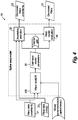
- Fig. 3 shows an exemplary data flow of the overall registration method 10.
- the image correlation process 18 done block-wise fashion across the image provides the warp estimates between the two bands, e.g. reference image 12 and warped image 14. These data estimates are noisy due to imperfect correlation and may be grossly off when the image content does not correlate well across the two spectral bands.
- the image correlation process may optionally also esimate the uncertainty associated with the estimated warp data.
- Any suitable method for estimating the warp and the associated uncertainty from image data can be used.
- These noisy warp data 20 estimates along with the uncertainty information 21 is fed to the separable spline warp model 16 to optimally filter the data (as explained above in Sec. 1) and correct the errors made in the image correlation process 18.
- the spline warp model produces reduced noise or de-noised warp estimates 22 and the associated uncertainty 23 with the data. These estimates may optionally be combined 25 with an independent warp estimate obtained from platform motion data to produce refined warp 27. Details of how the motion data is incoporated into the warp estimate is provided in Fig. 6 , as described below.
- the refined warp data 27 is then fed to an image resampling module 24 that resamples the warped band/image 14 to produce the final registered image 26.
- the internal data flow within the spline warp model 16 is shown in Fig. 4 .
- the warp model is first fitted 126 to the data 20 to obtain the unknown model parameters 28. If no uncertainty estimates are available for the warp data, the model fitting is performed using regular least squares as in eq. (13). If uncertainty estimates 21 are available, then either eqs. (17) or (19) are employed. If the input uncertainty estimates 21 are unreliable and the warp data has outliers, a robust fitting procedure is employed and eq. (23) is used after the robust fitting procedure has converged. If the smoothing model is employed for the spline coefficients then fitting is done using eq. (45) when the input uncertainty information is not available and eq.
- the warp model is then evaulated 30 at the grid locations required by the image resampling routine to dewarp the warped image 14 and register it to the reference image 12 (shown in Fig. 3 ).
- the estimated parameters 28 are used in eqs. (4), (5) and (6) to compute the slope, offset, and optical distortion profiles respectively and then eq. (3) is used to compute the de-noised warp 22 at the desired grid locations.
- the uncertainty of the de-noised warp 23 is predicted 32 using the fitted model parameters 28, the noisy warp data 20 and its associated uncertainty 21.
- Fig. 5 shows the details for the uncertainty estimation process 32 for predicting the uncertainty of the de-noised warp 22.
- robust fitting is performed, first the warp data uncertainties 21 are corrected 50 using the robust fitting weights 36 that identify the outliers to produce the corrected relative uncertainties 38.
- the robust fitting weights are given by eq. (30). This correction process is skipped if no robust fitting is performed.
- the fitted model parameters are used to obtain the filtering matrix in eq. (51), which is then applied to the corrected relative uncertainty 38 using eq. (52) by process 52 to obtain the de-noised warp relative uncertainty 40.
- the noise on the input warp data is estimated 42 by comparing the de-noised warp data 48, e.g., which can be the same as the de-noised warp 22 of Fig. 4 , to the input noisy warp data 20 with the knowledge of the fitted parameters 49, e.g., which can be the same as the parameters 28 of Fig. 4 , and the corrected relative uncertainty 38.
- the noise variance is estimated using eq. (60) when no robust fitting is performed and eqs. (62) or (63) is used when robust fitting is performed. This noise estimate is multiplied 54 with the de-noised warp relative uncertainty 40 to obtain the final de-noised warp uncertainty 23.
- Fig. 6 shows an exemplary embodiment where the de-noised warp uncertainty 23 of the predicted de-noised warp 22 can be utilized to further refine the warp if there is an alternate method of computing the warp.
- This refined warp 27 can be used instead of the de-noised warp 22 to perform the image resampling and register the warped image 14 with respect to the reference image 12.
- motion data 56 is available for the platform, e.g., an aircraft/space platform
- an estimate of the warp 60 between the reference and warp image can be obtained by utilizing a sensor model 58.
- a sensor model Such a method of using a sensor model to produce a warp is understood by those skilled in the art.
- the knowledge of the noise in the measurements of the platform motion can also be utilized to obtain the uncertainty 62 of the warp computed from the motion data 56. It has been explained above how the de-noised warp data and its associated uncertainty can be obtained from image data. These two independent estimates of the warps and their associated uncertainty can be optimally combined 29 to produce a final refined warp 27. Let denote the warp estimate obtained from motion data and let ⁇ ⁇ denote the associated uncertainty of this data.
- h ⁇ ⁇ ⁇ d ⁇ ⁇ 1 + ⁇ g ⁇ ⁇ 1 ⁇ 1 ⁇ d ⁇ ⁇ 1 d ⁇ ⁇ + ⁇ g ⁇ ⁇ 1 g ⁇ ⁇
- ⁇ d ⁇ is the associated uncertainty of this data obtained from eq. (54).
- a system for registering images can include a module configured to implement machine readable instructions to perform one or more of the method embodiments described above.
- aspects of the present embodiments may be embodied as a system, method or computer program product. Accordingly, aspects of the present embodiments may take the form of an entirely hardware embodiment, an entirely software embodiment (including firmware, resident software, micro-code, etc.) or an embodiment combining software and hardware aspects that may all generally be referred to herein as a "circuit,” “module” or “system.” Furthermore, aspects of the present disclosure may take the form of a computer program product embodied in one or more computer readable medium(s) having computer readable program code embodied thereon.
- the computer readable medium may be a computer readable signal medium or a computer readable storage medium.
- a computer readable storage medium may be, for example, but not limited to, an electronic, magnetic, optical, electromagnetic, infrared, or semiconductor system, apparatus, or device, or any suitable combination of the foregoing.
- a computer readable storage medium may be any tangible medium that can contain, or store a program for use by or in connection with an instruction execution system, apparatus, or device.
- a computer readable signal medium may include a propagated data signal with computer readable program code embodied therein, for example, in baseband or as part of a carrier wave. Such a propagated signal may take any of a variety of forms, including, but not limited to, electro-magnetic, optical, or any suitable combination thereof.
- a computer readable signal medium may be any computer readable medium that is not a computer readable storage medium and that can communicate, propagate, or transport a program for use by or in connection with an instruction execution system, apparatus, or device.
- Program code embodied on a computer readable medium may be transmitted using any appropriate medium, including but not limited to wireless, wireline, optical fiber cable, RF, etc., or any suitable combination of the foregoing.
- Computer program code for carrying out operations for aspects of the present disclosure may be written in any combination of one or more programming languages, including an object oriented programming language such as Java, Smalltalk, C++ or the like and conventional procedural programming languages, such as the "C" programming language or similar programming languages.
- the program code may execute entirely on the user's computer, partly on the user's computer, as a stand-alone software package, partly on the user's computer and partly on a remote computer or entirely on the remote computer or server.
- the remote computer may be connected to the user's computer through any type of network, including a local area network (LAN) or a wide area network (WAN), or the connection may be made to an external computer (for example, through the Internet using an Internet Service Provider).
- LAN local area network
- WAN wide area network
- Internet Service Provider for example, AT&T, MCI, Sprint, EarthLink, MSN, GTE, etc.
- These computer program instructions may also be stored in a computer readable medium that can direct a computer, other programmable data processing apparatus, or other devices to function in a particular manner, such that the instructions stored in the computer readable medium produce an article of manufacture including instructions which implement the function/act specified in the flowchart and/or block diagram block or blocks.
- the computer program instructions may also be loaded onto a computer, other programmable data processing apparatus, or other devices to cause a series of operational steps to be performed on the computer, other programmable apparatus or other devices to produce a computer implemented process such that the instructions which execute on the computer or other programmable apparatus provide processes for implementing the functions/acts specified in a flowchart and/or block diagram block or blocks
Landscapes
- Engineering & Computer Science (AREA)
- Physics & Mathematics (AREA)
- General Physics & Mathematics (AREA)
- Mathematical Physics (AREA)
- Theoretical Computer Science (AREA)
- Pure & Applied Mathematics (AREA)
- Data Mining & Analysis (AREA)
- Mathematical Analysis (AREA)
- Mathematical Optimization (AREA)
- Computational Mathematics (AREA)
- Algebra (AREA)
- Databases & Information Systems (AREA)
- Software Systems (AREA)
- General Engineering & Computer Science (AREA)
- Computer Vision & Pattern Recognition (AREA)
- Computing Systems (AREA)
- Operations Research (AREA)
- Image Processing (AREA)
- Gyroscopes (AREA)
- Studio Devices (AREA)
Abstract
Description
- This invention was made with government support under a Contract awarded by an agency. The government has certain rights in the invention.
- The present disclosure relates to imagery, and more particularly to registration of multiple images such as used in multi-modality and multi-spectral imagery.
- Registration between the different bands of multi-spectral imagery, e.g., acquired by an airborne or space sensor, is particularly challenging as the bands that are spectrally far apart do not correlate very well across the image. For example, bands deep in the IR region have both a reflective and an emissive component whereas the bands in the visual region are purely reflective.
- Simple phase correlation to obtain the warp is not very effective in these instances. Similarly, registering images acquired using different modalities such as LiDAR, narrow band spectral, and broad band visual photographic imagery present the same issues.
- Conventional methods and systems have generally been considered satisfactory for their intended purpose. However, there is still a need in the art for improved image registration for multi-modal and multi-spectral images. The present disclosure provides a solution for this need.
- A method for modeling warp for registration of images includes receiving input warp data and performing a fitting process on the input warp data to produce at least one of reduced noise warp data or reduced noise warp uncertainty. The warp for at the at least one of reduced noise warp data or reduced noise warp uncertainty is modeled with components including an offset that varies in time and a non-linear distortion that does not vary with time. The method also includes outputting at the least one of reduced noise warp data or reduced noise warp uncertainty.
- The warp can be modeled with components including a slope that varies in time. Performing the fitting process can include modeling the slope and offset as splines. Performing the fitting process can include modeling the non-linear distortion as a polynomial.
- The method can include receiving input warp data uncertainty for the input warp data, wherein performing the fitting process includes using the input warp data uncertainty in producing the reduced noise warp data. Performing the fitting process can include correcting errors in the input warp data uncertainty by performing a robust fitting process on the input warp data.
- The method can include predicting reduced noise warp uncertainty and utilizing the reduced noise warp uncertainty to generate a refined warp by incorporating motion data, and registering a warped band using the refined warp. It is also contemplated that the method can include predicting reduced noise warp uncertainty using the input warp data uncertainty and utilizing the reduced noise warp uncertainty to generate a refined warp by incorporating motion data, and registering a warped band using the refined warp.
- A sensor model can be used to produce warp data from motion and motion warp uncertainty, wherein the refined warp is produced by combining the reduced noise warp, the reduced noise warp uncertainty, the warp data from motion, and the motion warp uncertainty. Combining the reduced noise warp, the reduced noise warp uncertainty, the warp data from motion, and the motion warp uncertainty can include obtaining the refined warpas

 is the reduced noise warp, Σ d̂ is the reduced noise warp uncertainty,
 denotes the warp data from motion, and Σĝ denotes the motion warp uncertainty.
- The method can also include:
- using the input warp data uncertainty to produce relative input warp data uncertainty;
- using the relative input warp data uncertainty in a warp model robust fit to produce fit weights;
- using the fit weights and relative input warp data uncertainty to produce corrected relative input warp data uncertainty;
- predicting relative reduced noise warp data uncertainty from the corrected relative input warp data uncertainty;
- using the reduced noise warp data and the input warp data to estimate input noise variance; and
- multiplying the relative reduced noise warp data uncertainty and the input noise variance to produce the reduced noise warp data uncertainty.
- A smoothing model for slope and offset spline coefficients can be incorporated in the fitting process. Incorporating a smoothing model in the fitting process can include minimizing curvature of the offset and slope splines. The splines can have non-uniformly placed knots. The splines can be cubic.
- The fitting process can include modeling the warp as


- A method for registration of images includes receiving a reference image and a warped image, correlating the reference and warped images to produce noisy warp data, and performing a fitting process on the noisy warp data to produce reduced noise warp data. The warp for the reduced noise warp data is modeled with components including an offset that varies in time, and a non-linear distortion that does not vary with time. The method also includes resampling the warped image using the reduced noise warp data to produce a registered image that is registered to the reference image.
- Correlating the reference and warped images can include producing warp data uncertainty. Performing the fitting process can include generating reduced noise warp uncertainty. The method can include receiving motion data and combining the motion data with the reduced noise warp and the reduced noise warp uncertainty to produce a refined warp, wherein resampling the warped image using the reduced noise warp data includes using the refined warp to produce the registered image.
- A system includes a module configured to implement machine readable instructions to perform any embodiment of the methods described above.
- These and other features of the systems and methods of the subject disclosure will become more readily apparent to those skilled in the art from the following detailed description of the preferred embodiments taken in conjunction with the drawings.
- So that those skilled in the art to which the subject disclosure appertains will readily understand how to make and use the devices and methods of the subject disclosure without undue experimentation, preferred embodiments thereof will be described in detail herein below with reference to certain figures, wherein:
-
Figs. 1A-1D are a set of graphs showing spline basis functions in accordance with an exemplary embodiment of the present disclosure; -
Fig. 2 is a graph showing three exemplary functions for assigning weights to data samples in accordance with an exemplary embodiment of the present disclosure; -
Fig. 3 is a data flow diagram of an exemplary embodiment of image registration in accordance with the present disclosure; -
Fig. 4 is a data flow diagram of an exemplary embodiment of a method of modeling warp for image registration in accordance with the present disclosure; -
Fig. 5 is a data flow diagram of uncertainty estimation in accordance with an embodiment of the present disclosure; and -
Fig. 6 is a data flow diagram for an exemplary embodiment of estimating warp with motion data. - Reference will now be made to the drawings wherein like reference numerals identify similar structural features or aspects of the subject disclosure. For purposes of explanation and illustration, and not limitation, a partial view of an exemplary embodiment of a method in accordance with the disclosure is shown in
Fig. 3 and is designated generally byreference character 10. Other embodiments of methods in accordance with the disclosure, or aspects thereof, are provided inFigs. 1A-1D ,2 and4-6 , as will be described. The systems and methods described herein can be used for multi-modal/multi-spectral image registration. - Let {xw , yw } denote the coordinates in a warped band image that correspond to the coordinates {x, y} in a reference band image. Let


- In the subsequent treatment, we will use v = {x, y} as an index for x or y . Since the equations are similar for the translations in x and y , this makes for compact notation. Assuming the platform motion is more or less steady, the slope and offset, s ∗(·) and c ∗(·), will be smooth functions of time, y . We choose to model them as B-splines and they can written as a summation of a set of basis functions as


- The optical distortion can either be modeled as a B-spline or a polynomial


- To generate the B-spline functions, the number and location of the knots need to be specified along with the order of the spline. Let the knots sequence be denoted as t 1 ≤ t 2 ≤ ... ≤ tn , where n is the number of knots. Let k denote the order of the spline where k = 1 denotes the 0 th order spline. The B-spline basis functions for any order k is generated recursively from the previous order basis functions. The knots sequence is augmented for each order k as follows

- The recursion of the B-spline at any order k > 1 is given as


-
Figs. 1A-1D show this recursion from k = 1 to k = 4 to generate the cubic splines (k = 4) for a non-uniformly spaced knots sequence [0,0.25,0.4,0.8,1]. - The unknown spline coefficients for slope, offset, and optical distortion need to estimated. This is achieved by fitting the warping model Eq. (3) to the warping data obtained by the image correlation algorithm at a discrete set of tie points. To obtain the warp data at the tie points, methods such as phase correlation on local images of the warped band and the master band centered on the tie points may be empolyed. Such methods are known to those skilled in the art. Let {xi , yi }, i = 1,..., m denote a set of m grid points at which the warp has been estimated. To facilitate the estimation of the unknown coefficient, we rewrite Eq. (3) in vector-matrix notation


- Equation (10) compactly represents the warp model evaluated at the tie point grid where warping data is available either through image correlation or some other means. In general, the data from the image correlation process will be noisy either due to measurement process or correlation model mismatch as the image content may not match very well between the warped band and the master band. We would like to adjust the unknown spline coefficient to minimize the mean square error between the model predictions and the data. The least-squares estimate can be obtained in closed form and is given as

- The solution of Eq. (13) assumes that the noise is uniformly distributed across all the m data points and that the two components in x and y are independent. However, depending on how the data values are obtained for the warping, the noise may be quite variable between the data points and also coupled between the two components. Let W(i) denote the 2x2 weighting matrix for data point i based on the confidence we have on the estimate for that point. The inverse of the noise covariance matrix can be chosen as the weighting matrix. The weighted mean square error across all m data points in vector-matrix notation is given as


p and setting it equal to zero
- If the x and y components are uncorrelated (weighting matrices W(i) are diagonal), then Eq. (17) can be simplified since the spline coefficient for x and y can be estimated independently. Let


- The warping model matrix A can end up being badly scaled and ill-conditioned leading to a host of numerical issues in the solution of the model spline coefficients. The problem arises because the range of x and y may be large and quite different from each other. The large range of x makes the basis functions for the optical distortion model given by Eq. (6) to have a very large dynamic range if the polynomial model is chosen. With finite precision, the matrices will become rank deficient making it difficult to fit the data correctly. To overcome this problem, it is advisable to first normalize the range of the x and y between 0 and 1. The warping model is then fitted in the normalized domain and the results scaled back to the original domain for subsequent processing.
- Also note the solutions in Eqs. (13), (17), and (19), require a matrix inverse. Although they have been written in that form, it is not advisable to compute the explicit inverse both from a numerical accuracy and performance considerations. Instead, it is better to take the inverted matrix to the other side of the equation and solve the resulting set of linear equations using Gaussian elimination.
- The previous Sections assumes that the noise in the data can be modeled as Gaussian. However, in practice if the data are generated using an image correlation procedure, the noise is very much image content dependent. Furthermore, if the image registration is being done between two different imaging modalities or very different spectral bands, the image correlation model may break down. Both of these factors can lead to large impulsive kind of noise that is not very well modeled by a unimodal normal distribution. The quadratic penalty resulting from the Gaussian assumption tends to be overly sensitive to outliers and the resulting least-squares solution can end up significantly biased. Towards this end, we would like to replace the quadratic penalty with alternative penalty functions that reduce the cost the model associates with large outlying values in the data. The optimal shape of the penalty function is given by actual probability distribution function of the noise in the data. In practice, it is difficult to come up with an accurate description of the noise. However, any penalty function that reduces the cost associated with large outlying values will tend to perform better in the case the data is corrupted by impulsive or heavier tail distributions.
- One advantage of the weighted least squares method is that the solution comes out to be closed form. This will not be case if an alternative robust penalty function is employed. However, we can leverage the closed form solution for weighted least squares to come up with an iterative solution that assigns varying weights to each data point based on a determination of how well it fits the Gaussian distribution assumption. The weights vary during the iterative process as the model moves to fit the normally distributed data points and reject the outlying data values that do not fit the model very well.
- This Section lays out the robust solution when the x and y components are uncorrelated. In this case, the model fitting in x and y can be carried out independently. For notational simplicity, we will drop the subscripts x and y on the matrices in this Section and give the robust solution for the general problem

d is the data vector andp is the vector of unknown model coefficients. Note that the general formulation given by Eq. (21) includes the case where we have a weighting matrix W. The effect of the weighting is incorporated in the model matrix and the data vector as follows:
- The robust fitting method proceeds by assigning weights to each of the data points at each iteration based on its determination of how likely the point is an outlier or not. Let l denote the iteration index and let


- The normalized residuals are then passed through a weighting function ρ(·) that assigns weights to each data sample. For robustness, we would like to dial down the weights as the normalized residual gets large signaling an outlier. There are numerous functions in the literature that achieve this purpose.
Fig. 2 shows three of the most commonly used functions for this purpose. Large residual error signals a model misfit and is given lower weight in the fitting process to achieve robustness to outliers. We will use the bisquare function given as

Fig. 2 . - The procedure outlined in this Section is repeated until the estimate of the unknown model coefficients given by Eq. (23) converges or the maximum number of iterations are exceeded.
- The smoothness of the slope and offset profiles in time is implicitly determined by the choice of the number of spline coefficients and their placement. A small number of evenly spaced knots constrains the profiles to be smooth. Increasing the number of knots frees up the profiles to change more quickly. Ideally, we would like the splines to be flexible enough to fit all the good data. However, choosing a large number of knots can make the results vary wildly in areas where there is no data to constrain the solution. The numerical solutions proposed in Section 1.2 do not guarantee a minimum norm solution.
- The implicit specification of smoothing is undesirable since it shifts the difficultly to optimal estimation of the number and placement of knots. Instead, we use an explicit smoothing model in the optimization problem. The original cost function minimized the mean square error between the model and the data. We add to this function a roughness penalty that will favor smoother solutions. We formulate the roughness penalty as the integrated square of the second derivative of the slope and offset functions given as


notation 0 ns xno denotes a ns x no matrix of all zeros. The overall cost function to be minimized for the x and y model is given as


W v denotes the weight matrix augmented by the weights for the smoothing constraints
- To obtain a robust solution, the prescription given in Sec. 1.2.6 can be followed using the augmented model matrix
A and data vectord with the user supplied weights folded in. Note that this will treat the additional ns + nc constraints given by matrix D as data points and obtain robust weights for them depending on how well the constraints can be satisfied. If this is not desirable, then a procedure similar to that outlined in Sec. 1.2.6 can be formulated that obtains robust weights for only the data points and then computes the model parameters using the robust weights and the smoothing model. - In this Section,the subscript v denoting x or y will be dropped for notational simplicity as the equations are same for both x and y . E[·] denotes the expectation operator and bold case is used to specify the random variables over which the expectation is computed and for denoting matrices. Since the expectation in this Section is always computed on vectors (denoted with →), there should be no confusion between the two. Estimated quantities will be denoted by a ^ and matrices and vectors augmented by the smoothing constraints denoted by a-.
- We are interested in computing the expected mean square error (MSE) between the warp model predictionsand the ground truth warp

d t as a measure of accuracy of the model output. In practice, the ground truth warp is not available but it will not be required if the model predictions are unbiased as shown below
- Assuming the warp formulated in Sec. 1 models physical reality closely, the model predictions based on image correlation data will be unbiased making Eq. (49) valid. In practice, the bias term will be small and the covariance of the model output will accurately predict the MSE.
- We will derive the expression for Σ d̂ for the most general case including the smoothing model and robust fitting. Reducing to the special cases of no smoothing model with and without robust fitting is then trivial. Let W denote the weighting matrix for the data points that is obtained by multiplying the specified weights (if any), which are ideally set to the inverse covariance matrix of the input data for optimality, with the weights obtained during robust fitting (if enabled). If the input data has no specified weights and robust fitting is not performed, this will be the identity matrix. As before,
W denotes the augmented matrix with the smoothing weights included if the smoothing model is employed. Then the model prediction can be obtained using Eqs. (10) and (47)


d is the covariance of the input augmented data. If we trust the input data covariance supplied by the user (no robust fitting performed), Eq. (52) gives us the covariance of the prediction for the most general case. - However, in practice, the input data covariance estimated from image correlation process may be inaccurate for some number of points. The robust fitting procedure of Sec. 1.2.5 is designed precisely to identity such outlier data points. The robust fitting weights can be regarded as corrections to the weights derived from the supplied input data covariance matrix. In essence, the overall weight matrix
W , which includes the robust fitting weights, is a refined estimate of the inverse covariance of the input data up to a scale factor. The absolute scale of the input covariance cannot be estimated as part of the robust fitting procedure since only the relative weights between the data points matter in the fitting procedure. In practice, the data weights are usually normalized to unity mean to make them unitless. This makes it easier to specify a fixed amount of smoothing through the smoothing weights independent of the scale of the input data. The estimated input data covariance in terms of the weights is given as


- 1.4.1 Estimation of

- The residual of the augmented data is given as


F Σd =F Σd F t . Rearranging the terms in Eq. (57) gives


F is a full matrix, the residuals are very strongly correlated (at least locally) and nowhere close to independent. However, in practice, approximating the residuals to be independent for the purpose of estimating
F , which is a large (m + na )x(m + na ) matrix. There are numerical issues involved in the inversion of I -F as well since it does not have full rank. A pseudo inverse can be employed but in practice it is better to approximate it as a diagonal matrix and just invert the diagonal entries for the purpose of estimating scale. Approximating independence and restricting the trace to the data portion yields
- 1.4.2 Unbiased estimate of

- The noise estimate given by Eq. (60) can potentially be biased lower when robust fitting is performed. Large outliers are suppressed by dialing down the robust weights but in the process other sample points that fall in the true distribution are also de-weighted significantly if they are far away from the mean of the distribution. The exact expression for the bias is difficult to compute analytically when robust fitting is performed without making simplifying assumptions that are typically not valid in practice. Instead, we will use our intuition to come up with a correction factor that accounts for this bias and verify the resulting expression via Monte Carlo simulations.
- When computing statistics from N independent samples, we know that the variance of the esimated statistic goes down as 1/N, i.e., each sample has an effective contribution of 1. In robust fitting, we have a weight assigned to each sample i at iteration l,


- Also, note that an estimate of the input data noise similar to that given by Eq. (60) was obtained as part of robust fitting. See Sec. 1.2.6 and the robust estimate of noise given by Eq. (28). We can utilize this estimate along with the heuristic correction factor K to obtain an unbiased estimate


-
Fig. 3 shows an exemplary data flow of theoverall registration method 10. Theimage correlation process 18 done block-wise fashion across the image provides the warp estimates between the two bands,e.g. reference image 12 andwarped image 14. These data estimates are noisy due to imperfect correlation and may be grossly off when the image content does not correlate well across the two spectral bands. The image correlation process may optionally also esimate the uncertainty associated with the estimated warp data. Those skilled in the art will readily appreciate that that any suitable method for estimating the warp and the associated uncertainty from image data can be used. Thesenoisy warp data 20 estimates along with theuncertainty information 21 is fed to the separablespline warp model 16 to optimally filter the data (as explained above in Sec. 1) and correct the errors made in theimage correlation process 18. Details of this estimation process are provided inFigs. 4 and5 as described below. The spline warp model produces reduced noise or de-noised warp estimates 22 and the associateduncertainty 23 with the data. These estimates may optionally be combined 25 with an independent warp estimate obtained from platform motion data to produce refinedwarp 27. Details of how the motion data is incoporated into the warp estimate is provided inFig. 6 , as described below. Therefined warp data 27 is then fed to animage resampling module 24 that resamples the warped band/image 14 to produce the finalregistered image 26. - The internal data flow within the
spline warp model 16 is shown inFig. 4 . The warp model is first fitted 126 to thedata 20 to obtain theunknown model parameters 28. If no uncertainty estimates are available for the warp data, the model fitting is performed using regular least squares as in eq. (13). If uncertainty estimates 21 are available, then either eqs. (17) or (19) are employed. If the input uncertainty estimates 21 are unreliable and the warp data has outliers, a robust fitting procedure is employed and eq. (23) is used after the robust fitting procedure has converged. If the smoothing model is employed for the spline coefficients then fitting is done using eq. (45) when the input uncertainty information is not available and eq. (47) when either the input uncertainty is available or reconstructed using robust fitting. The warp model is then evaulated 30 at the grid locations required by the image resampling routine to dewarp thewarped image 14 and register it to the reference image 12 (shown inFig. 3 ). The estimatedparameters 28 are used in eqs. (4), (5) and (6) to compute the slope, offset, and optical distortion profiles respectively and then eq. (3) is used to compute thede-noised warp 22 at the desired grid locations. The uncertainty of thede-noised warp 23 is predicted 32 using the fittedmodel parameters 28, thenoisy warp data 20 and its associateduncertainty 21. -
Fig. 5 shows the details for theuncertainty estimation process 32 for predicting the uncertainty of thede-noised warp 22. If robust fitting is performed, first thewarp data uncertainties 21 are corrected 50 using the robustfitting weights 36 that identify the outliers to produce the correctedrelative uncertainties 38. The robust fitting weights are given by eq. (30). This correction process is skipped if no robust fitting is performed. The fitted model parameters are used to obtain the filtering matrix in eq. (51), which is then applied to the correctedrelative uncertainty 38 using eq. (52) byprocess 52 to obtain the de-noised warprelative uncertainty 40. Finally, the noise on the input warp data is estimated 42 by comparing thede-noised warp data 48, e.g., which can be the same as thede-noised warp 22 ofFig. 4 , to the inputnoisy warp data 20 with the knowledge of the fittedparameters 49, e.g., which can be the same as theparameters 28 ofFig. 4 , and the correctedrelative uncertainty 38. In particular, the noise variance is estimated using eq. (60) when no robust fitting is performed and eqs. (62) or (63) is used when robust fitting is performed. This noise estimate is multiplied 54 with the de-noised warprelative uncertainty 40 to obtain the finalde-noised warp uncertainty 23. -
Fig. 6 shows an exemplary embodiment where thede-noised warp uncertainty 23 of the predictedde-noised warp 22 can be utilized to further refine the warp if there is an alternate method of computing the warp. Thisrefined warp 27 can be used instead of thede-noised warp 22 to perform the image resampling and register thewarped image 14 with respect to thereference image 12. Ifmotion data 56 is available for the platform, e.g., an aircraft/space platform, an estimate of thewarp 60 between the reference and warp image can be obtained by utilizing asensor model 58. Such a method of using a sensor model to produce a warp is understood by those skilled in the art. The knowledge of the noise in the measurements of the platform motion can also be utilized to obtain theuncertainty 62 of the warp computed from themotion data 56. It has been explained above how the de-noised warp data and its associated uncertainty can be obtained from image data. These two independent estimates of the warps and their associated uncertainty can be optimally combined 29 to produce a finalrefined warp 27. Letdenote the warp estimate obtained from motion data and let Σ ĝ denote the associated uncertainty of this data. Then the optimal estimate of the overall warp (refined warp) is obtained as
 is the de-noised warp estimate from image data obtained from eq. (50) and Σ d̂ is the associated uncertainty of this data obtained from eq. (54).
- Those skilled in the art will readily appreciate that a system for registering images can include a module configured to implement machine readable instructions to perform one or more of the method embodiments described above.
- As will be appreciated by those skilled in the art, aspects of the present embodiments may be embodied as a system, method or computer program product. Accordingly, aspects of the present embodiments may take the form of an entirely hardware embodiment, an entirely software embodiment (including firmware, resident software, micro-code, etc.) or an embodiment combining software and hardware aspects that may all generally be referred to herein as a "circuit," "module" or "system." Furthermore, aspects of the present disclosure may take the form of a computer program product embodied in one or more computer readable medium(s) having computer readable program code embodied thereon.
- Any combination of one or more computer readable medium(s) may be utilized. The computer readable medium may be a computer readable signal medium or a computer readable storage medium. A computer readable storage medium may be, for example, but not limited to, an electronic, magnetic, optical, electromagnetic, infrared, or semiconductor system, apparatus, or device, or any suitable combination of the foregoing. More specific examples (a non-exhaustive list) of the computer readable storage medium would include the following: an electrical connection having one or more wires, a portable computer diskette, a hard disk, a random access memory (RAM), a read-only memory (ROM), an erasable programmable read-only memory (EPROM or Flash memory), an optical fiber, a portable compact disc read-only memory (CD-ROM), an optical storage device, a magnetic storage device, or any suitable combination of the foregoing. In the context of this document, a computer readable storage medium may be any tangible medium that can contain, or store a program for use by or in connection with an instruction execution system, apparatus, or device.
- A computer readable signal medium may include a propagated data signal with computer readable program code embodied therein, for example, in baseband or as part of a carrier wave. Such a propagated signal may take any of a variety of forms, including, but not limited to, electro-magnetic, optical, or any suitable combination thereof. A computer readable signal medium may be any computer readable medium that is not a computer readable storage medium and that can communicate, propagate, or transport a program for use by or in connection with an instruction execution system, apparatus, or device.
- Program code embodied on a computer readable medium may be transmitted using any appropriate medium, including but not limited to wireless, wireline, optical fiber cable, RF, etc., or any suitable combination of the foregoing.
- Computer program code for carrying out operations for aspects of the present disclosure may be written in any combination of one or more programming languages, including an object oriented programming language such as Java, Smalltalk, C++ or the like and conventional procedural programming languages, such as the "C" programming language or similar programming languages. The program code may execute entirely on the user's computer, partly on the user's computer, as a stand-alone software package, partly on the user's computer and partly on a remote computer or entirely on the remote computer or server. In the latter scenario, the remote computer may be connected to the user's computer through any type of network, including a local area network (LAN) or a wide area network (WAN), or the connection may be made to an external computer (for example, through the Internet using an Internet Service Provider).
- Aspects of the present disclosure are described above with reference to flowchart illustrations and/or block diagrams of methods, apparatus (systems) and computer program products according to embodiments of the embodiments. It will be understood that each block of the flowchart illustrations and/or block diagrams, and combinations of blocks in the flowchart illustrations and/or block diagrams, can be implemented by computer program instructions. These computer program instructions may be provided to a processor of a general purpose computer, special purpose computer, or other programmable data processing apparatus to produce a machine, such that the instructions, which execute via the processor of the computer or other programmable data processing apparatus, create means for implementing the functions/acts specified in the flowchart and/or block diagram block or blocks.
- These computer program instructions may also be stored in a computer readable medium that can direct a computer, other programmable data processing apparatus, or other devices to function in a particular manner, such that the instructions stored in the computer readable medium produce an article of manufacture including instructions which implement the function/act specified in the flowchart and/or block diagram block or blocks.
- The computer program instructions may also be loaded onto a computer, other programmable data processing apparatus, or other devices to cause a series of operational steps to be performed on the computer, other programmable apparatus or other devices to produce a computer implemented process such that the instructions which execute on the computer or other programmable apparatus provide processes for implementing the functions/acts specified in a flowchart and/or block diagram block or blocks
- The methods and systems of the present disclosure, as described above and shown in the drawings, provide for imagery with superior properties including improved multi-band/multi-spectral image registration. While the apparatus and methods of the subject disclosure have been shown and described with reference to preferred embodiments, those skilled in the art will readily appreciate that changes and/or modifications may be made thereto without departing from the scope of the subject disclosure.
Claims (15)
- A method for modeling warp for registration of images comprising:receiving input warp data; andperforming a fitting process on the input warp data to produce at least one of reduced noise warp data or reduced noise warp uncertainty, wherein the warp for at the at least one of reduced noise warp data or reduced noise warp uncertainty is modeled with components including:an offset that varies in time; anda non-linear distortion that does not vary with time; andoutputting the at least one of reduced noise warp data or reduced noise warp uncertainty.
- A method as recited in claim 1, wherein the warp is modeled with components including a slope that varies in time;
optionally wherein performing the fitting process includes modeling the slope and offset as splines and/or wherein performing the fitting process includes modeling the non-linear distortion as a polynomial. - A method as recited in claim 1 or 2, further comprising:receiving input warp data uncertainty for the input warp data, wherein performing the fitting process includes using the input warp data uncertainty in producing the reduced noise warp data.
- A method as recited in claim 3, wherein performing the fitting process includes correcting errors in the input warp data uncertainty by performing a robust fitting process on the input warp data.
- A method as recited in any preceding claim, further comprising:predicting reduced noise warp uncertainty and utilizing the reduced noise warp uncertainty to generate a refined warp by incorporating motion data; andregistering a warped band using the refined warp;optionally wherein the step of predicting reduced noise warp uncertainty uses the input warp data uncertainty.
- A method as recited in claim 5, using a sensor model to produce warp data from motion and motion warp uncertainty, wherein the refined warp is produced by combining the reduced noise warp, the reduced noise warp uncertainty, the warp data from motion, and the motion warp uncertainty;
optionally wherein combining the reduced noise warp, the reduced noise warp uncertainty, the warp data from motion, and the motion warp uncertainty includes obtaining the refined warpas
 denotes the warp data from motion, and Σ ĝ denotes the motion warp uncertainty.
- A method as recited in claim 3, further comprising
using the input warp data uncertainty to produce relative input warp data uncertainty;
using the relative input warp data uncertainty in a warp model robust fit to produce fit weights;
using the fit weights and relative input warp data uncertainty to produce corrected relative input warp data uncertainty;
predicting relative reduced noise warp data uncertainty from the corrected relative input warp data uncertainty;
using the reduced noise warp data and the input warp data to estimate input noise variance; and
multiplying the relative reduced noise warp data uncertainty and the input noise variance to produce the reduced noise warp data uncertainty. - A method as recited in claim 2, wherein a smoothing model for slope and offset spline coefficients is incorporated in the fitting process; optionally wherein incorporating a smoothing model in the fitting process includes minimizing curvature of the offset and slope splines.
- A method as recited in claim 2, wherein the splines have non-uniformly placed knots, or wherein the splines are cubic.
- A method as recited in claim 2, wherein the fitting process includes modeling the warp as


- A system including:a module configured to implement machine readable instructions to perform the method recited in any preceding claim.
- A system as recited in claim 11, wherein the module is configured to implement machine readable instructions including instructions to:receive a reference image and a warped image;correlate the reference and warped images to produce noisy warp data;perform a fitting process on the noisy warp data to produce reduced noise warp data,wherein the warp for the reduced noise warp data is modeled with components including:an offset that varies in time; anda non-linear distortion that does not vary with time; andresampling the warped image using the reduced noise warp data to produce a registered image that is registered to the reference image.
- A method for registration of images comprising:receiving a reference image and a warped image;correlating the reference and warped images to produce noisy warp data;performing a fitting process on the noisy warp data to produce reduced noise warp data, wherein the warp for the reduced noise warp data is modeled with components including:an offset that varies in time; anda non-linear distortion that does not vary with time; andresampling the warped image using the reduced noise warp data to produce a registered image that is registered to the reference image.
- A method as recited in claim 13, wherein correlating the reference and warped images includes producing warp data uncertainty and/or wherein performing the fitting process includes generating reduced noise warp uncertainty.
- A method as recited in claim 14, further comprising:receiving motion data; andcombining the motion data with the reduced noise warp and the reduced noise warp uncertainty to produce a refined warp, wherein resampling the warped image using the reduced noise warp data includes using the refined warp to produce the registered image.
Applications Claiming Priority (1)
| Application Number | Priority Date | Filing Date | Title |
|---|---|---|---|
| US15/094,123 US10223331B2 (en) | 2016-04-08 | 2016-04-08 | Warp models for registering multi-spectral imagery |
Publications (2)
| Publication Number | Publication Date |
|---|---|
| EP3229207A2 true EP3229207A2 (en) | 2017-10-11 |
| EP3229207A3 EP3229207A3 (en) | 2017-11-15 |
Family
ID=58464173
Family Applications (1)
| Application Number | Title | Priority Date | Filing Date |
|---|---|---|---|
| EP17162280.6A Pending EP3229207A3 (en) | 2016-04-08 | 2017-03-22 | Warp models for registering multi-spectral imagery |
Country Status (2)
| Country | Link |
|---|---|
| US (1) | US10223331B2 (en) |
| EP (1) | EP3229207A3 (en) |
Cited By (3)
| Publication number | Priority date | Publication date | Assignee | Title |
|---|---|---|---|---|
| CN110213325A (en) * | 2019-04-02 | 2019-09-06 | 腾讯科技(深圳)有限公司 | Data processing method and data push method |
| CN112100574A (en) * | 2020-08-21 | 2020-12-18 | 西安交通大学 | Resampling-based AAKR model uncertainty calculation method and system |
| CN112927161A (en) * | 2021-03-12 | 2021-06-08 | 新疆大学 | Method and device for enhancing multispectral remote sensing image and storage medium |
Families Citing this family (1)
| Publication number | Priority date | Publication date | Assignee | Title |
|---|---|---|---|---|
| CN109255171B (en) * | 2018-08-29 | 2023-09-05 | 深圳十沣科技有限公司 | Method for automatically judging convergence of numerical simulation calculation |
Family Cites Families (12)
| Publication number | Priority date | Publication date | Assignee | Title |
|---|---|---|---|---|
| US7298869B1 (en) | 2003-07-21 | 2007-11-20 | Abernathy Donald A | Multispectral data acquisition system and method |
| JP4072108B2 (en) | 2003-10-07 | 2008-04-09 | オリンパス株式会社 | Image display device and image display method |
| US7298922B1 (en) | 2004-07-07 | 2007-11-20 | Lockheed Martin Corporation | Synthetic panchromatic imagery method and system |
| FR2879791B1 (en) | 2004-12-16 | 2007-03-16 | Cnes Epic | METHOD FOR PROCESSING IMAGES USING AUTOMATIC GEOREFERENCING OF IMAGES FROM A COUPLE OF IMAGES TAKEN IN THE SAME FOCAL PLAN |
| US7813586B2 (en) | 2006-08-07 | 2010-10-12 | Mela Sciences, Inc. | Reducing noise in digital images |
| KR100944462B1 (en) | 2008-03-07 | 2010-03-03 | 한국항공우주연구원 | Satellite image fusion method and system |
| US8194952B2 (en) * | 2008-06-04 | 2012-06-05 | Raytheon Company | Image processing system and methods for aligning skin features for early skin cancer detection systems |
| US9635285B2 (en) | 2009-03-02 | 2017-04-25 | Flir Systems, Inc. | Infrared imaging enhancement with fusion |
| EP2567359B1 (en) * | 2010-05-06 | 2014-10-29 | Koninklijke Philips N.V. | Image data registration for dynamic perfusion ct |
| US9223021B2 (en) | 2012-10-22 | 2015-12-29 | The United States Of America As Represented By The Secretary Of The Army | Method and system for motion compensated target detection using acoustical focusing |
| US9483816B2 (en) | 2013-09-03 | 2016-11-01 | Litel Instruments | Method and system for high accuracy and reliability registration of multi modal imagery |
| AU2015202937A1 (en) * | 2015-05-29 | 2016-12-15 | Canon Kabushiki Kaisha | Systems and methods for registration of images |
-
2016
- 2016-04-08 US US15/094,123 patent/US10223331B2/en active Active
-
2017
- 2017-03-22 EP EP17162280.6A patent/EP3229207A3/en active Pending
Non-Patent Citations (1)
| Title |
|---|
| None |
Cited By (4)
| Publication number | Priority date | Publication date | Assignee | Title |
|---|---|---|---|---|
| CN110213325A (en) * | 2019-04-02 | 2019-09-06 | 腾讯科技(深圳)有限公司 | Data processing method and data push method |
| CN112100574A (en) * | 2020-08-21 | 2020-12-18 | 西安交通大学 | Resampling-based AAKR model uncertainty calculation method and system |
| CN112927161A (en) * | 2021-03-12 | 2021-06-08 | 新疆大学 | Method and device for enhancing multispectral remote sensing image and storage medium |
| CN112927161B (en) * | 2021-03-12 | 2022-07-01 | 新疆大学 | Method and device for enhancing multispectral remote sensing image and storage medium |
Also Published As
| Publication number | Publication date |
|---|---|
| US10223331B2 (en) | 2019-03-05 |
| US20170293590A1 (en) | 2017-10-12 |
| EP3229207A3 (en) | 2017-11-15 |
Similar Documents
| Publication | Publication Date | Title |
|---|---|---|
| Carron et al. | Maximum a posteriori CMB lensing reconstruction | |
| EP3229207A2 (en) | Warp models for registering multi-spectral imagery | |
| Tasse | Nonlinear Kalman filters for calibration in radio interferometry | |
| Rau et al. | A multi-scale multi-frequency deconvolution algorithm for synthesis imaging in radio interferometry | |
| Wang et al. | Kalman filtering through the feedback adaption of prior error covariance | |
| US8532951B2 (en) | Method for calibrating a transducer array | |
| Stompor et al. | Making maps of the cosmic microwave background: The MAXIMA example | |
| CN100583144C (en) | Multi-frame self-adaptive optical image high-resolution restoration method by using wavefront data | |
| Bocquet et al. | Expanding the validity of the ensemble Kalman filter without the intrinsic need for inflation | |
| Xu et al. | A refined strategy for removing composite errors of SAR interferogram | |
| US20190251215A1 (en) | Accurate estimation of upper atmospheric density using satellite observations | |
| Fisher | Estimation of entropy reduction and degrees of freedom for signal for large variational analysis systems | |
| US10769801B2 (en) | Fast multi-spectral image registration by modeling platform motion | |
| CN110688763A (en) | Multipath effect compensation method based on depth and light intensity images of pulse type ToF camera | |
| Reyes et al. | A variable high-order shock-capturing finite difference method with GP-WENO | |
| US20210241428A1 (en) | Image Reconstruction using Artificial Intelligence (Ai) Modules Agnostic to Image Acquisition Settings | |
| Wang et al. | Location and estimation of multiple outliers in weighted total least squares | |
| Morgan et al. | Sites: Solar iterative temperature emission solver for differential emission measure inversion of EUV observations | |
| Hólm | Lecture notes on assimilation algorithms | |
| Chang et al. | A composite likelihood approach to computer model calibration with high-dimensional spatial data | |
| Li et al. | Single image noise level estimation by artificial noise | |
| Bevilacqua et al. | Whiteness-based parameter selection for Poisson data in variational image processing | |
| Dautov et al. | Abstract theory of hybridizable discontinuous Galerkin methods for second-order quasilinear elliptic problems | |
| Wang et al. | A robust direction-of-arrival estimation method for impulsive noise environments | |
| WO2019104702A1 (en) | Adaptive joint sparse coding-based parallel magnetic resonance imaging method and apparatus and computer readable medium |
Legal Events
| Date | Code | Title | Description |
|---|---|---|---|
| PUAI | Public reference made under article 153(3) epc to a published international application that has entered the european phase |
Free format text: ORIGINAL CODE: 0009012 |
|
| STAA | Information on the status of an ep patent application or granted ep patent |
Free format text: STATUS: THE APPLICATION HAS BEEN PUBLISHED |
|
| AK | Designated contracting states |
Kind code of ref document: A2 Designated state(s): AL AT BE BG CH CY CZ DE DK EE ES FI FR GB GR HR HU IE IS IT LI LT LU LV MC MK MT NL NO PL PT RO RS SE SI SK SM TR |
|
| AX | Request for extension of the european patent |
Extension state: BA ME |
|
| PUAL | Search report despatched |
Free format text: ORIGINAL CODE: 0009013 |
|
| AK | Designated contracting states |
Kind code of ref document: A3 Designated state(s): AL AT BE BG CH CY CZ DE DK EE ES FI FR GB GR HR HU IE IS IT LI LT LU LV MC MK MT NL NO PL PT RO RS SE SI SK SM TR |
|
| AX | Request for extension of the european patent |
Extension state: BA ME |
|
| RIC1 | Information provided on ipc code assigned before grant |
Ipc: G06T 7/32 20170101AFI20171012BHEP |
|
| STAA | Information on the status of an ep patent application or granted ep patent |
Free format text: STATUS: REQUEST FOR EXAMINATION WAS MADE |
|
| 17P | Request for examination filed |
Effective date: 20180515 |
|
| RBV | Designated contracting states (corrected) |
Designated state(s): AL AT BE BG CH CY CZ DE DK EE ES FI FR GB GR HR HU IE IS IT LI LT LU LV MC MK MT NL NO PL PT RO RS SE SI SK SM TR |
|
| STAA | Information on the status of an ep patent application or granted ep patent |
Free format text: STATUS: EXAMINATION IS IN PROGRESS |
|
| 17Q | First examination report despatched |
Effective date: 20210211 |
|
| STAA | Information on the status of an ep patent application or granted ep patent |
Free format text: STATUS: EXAMINATION IS IN PROGRESS |
|
| P01 | Opt-out of the competence of the unified patent court (upc) registered |
Effective date: 20230922 |