EP3040887A1 - Magnetization analysis apparatus, magnetization analysis method, and magnetization analysis program - Google Patents
Magnetization analysis apparatus, magnetization analysis method, and magnetization analysis program Download PDFInfo
- Publication number
- EP3040887A1 EP3040887A1 EP15172063.8A EP15172063A EP3040887A1 EP 3040887 A1 EP3040887 A1 EP 3040887A1 EP 15172063 A EP15172063 A EP 15172063A EP 3040887 A1 EP3040887 A1 EP 3040887A1
- Authority
- EP
- European Patent Office
- Prior art keywords
- magnetization
- calculation unit
- field
- vector
- magnetic field
- Prior art date
- Legal status (The legal status is an assumption and is not a legal conclusion. Google has not performed a legal analysis and makes no representation as to the accuracy of the status listed.)
- Withdrawn
Links
Images


Classifications
-
- G—PHYSICS
- G06—COMPUTING OR CALCULATING; COUNTING
- G06F—ELECTRIC DIGITAL DATA PROCESSING
- G06F30/00—Computer-aided design [CAD]
- G06F30/20—Design optimisation, verification or simulation
- G06F30/23—Design optimisation, verification or simulation using finite element methods [FEM] or finite difference methods [FDM]
-
- G—PHYSICS
- G01—MEASURING; TESTING
- G01R—MEASURING ELECTRIC VARIABLES; MEASURING MAGNETIC VARIABLES
- G01R33/00—Arrangements or instruments for measuring magnetic variables
-
- G—PHYSICS
- G01—MEASURING; TESTING
- G01R—MEASURING ELECTRIC VARIABLES; MEASURING MAGNETIC VARIABLES
- G01R33/00—Arrangements or instruments for measuring magnetic variables
- G01R33/0064—Arrangements or instruments for measuring magnetic variables comprising means for performing simulations, e.g. of the magnetic variable to be measured
-
- G—PHYSICS
- G06—COMPUTING OR CALCULATING; COUNTING
- G06F—ELECTRIC DIGITAL DATA PROCESSING
- G06F2111/00—Details relating to CAD techniques
- G06F2111/10—Numerical modelling
Definitions
- the embodiments discussed herein are related to a magnetization analysis apparatus, a magnetization analysis method, and a computer-readable recording medium.
- Micromagnetic simulation in which a magnetic substance is modeled as an assembly of small magnets and the domain state is numerically simulated is known as a technology for analyzing the magnetization behavior of a magnetic substance.
- Micromagnetic simulation is used to analyze the domain state of a micromagnetic device, such as a magnetic head of a hard disk drive (HDD) or a magnetoresistive random access memory (MRAM), and a magnetic material, such as a permanent magnet or a magnetic steel sheet.
- a micromagnetic device such as a magnetic head of a hard disk drive (HDD) or a magnetoresistive random access memory (MRAM)
- MRAM magnetoresistive random access memory
- FIG. 13 is a diagram for explaining modeling of a magnetic substance by micromagnetization.
- the micromagnetization refers to individual small magnets.
- a magnetic vector 92 is calculated per micromagnetization 91 in micromagnetic simulation.
- the mesh size is adjusted such that the angles formed by magnetization vectors of meshes adjacent to each other are small angles so that the magnetization directions are regarded as approximately continuous.
- the mesh size is requested to be smaller than an exchange length.
- the exchange length decreases to approximately one nanometer (nm).
- the exchange length represents the diameter of a crystal grain where an exchange occurs.
- an effective magnetic field that acts on each element to be analyzed is calculated using, as a fixed value, a magnetic field calculated by magnetic field analysis using a finite element method and a magnetization vector in each element is calculated using the calculated effective magnetic field, so that the speed of analyzing the characteristics of a magnetic substance is increased.
- Micromagnetic simulation has a problem in that an increase in the mesh size worsens the calculation accuracy. For this reason, a technology that allows accurate simulations even with a mesh size that worsens the calculation accuracy is important.
- a magnetization analysis apparatus includes: an intermediate magnetization calculation unit that calculates, using a magnetization vector of each of elements obtained by mesh division in which a magnetic substance is divided into a plurality of meshes and a magnetization vector of an element adjacent to each element, intermediate magnetization that is a magnetization vector at the halfway point between each element and an element adjacent to each element; an effective magnetic field calculation unit that calculates an effective magnetic field using the intermediate magnetization calculated by the intermediate magnetization calculation unit; and a magnetization calculation unit that calculates a magnetization vector of each element after a unit time based on the effective magnetic field calculated by the effective magnetic field calculation unit.
- the magnetization analysis apparatus is an apparatus that performs micromagnetic simulations and that calculates a magnetization vector for a given time at each given time step and displays the magnetization vector.
- the present invention is not limited to the embodiment and it can be widely applied to magnetization analysis.
- FIG. 1 is a functional block diagram illustrating a configuration of a magnetization analysis apparatus according to the embodiment.
- a magnetization apparatus 1 includes an input unit 2, a display unit 3, a storage unit 4, and a control unit 5.
- the input unit 2 is an input device for a user who performs an analysis to input various types of information and instructions to the magnetization analysis apparatus 1.
- the input unit 2 corresponds to a keyboard, a mouse, and a touch panel.
- the display unit 3 is a display device that displays various types of information.
- the display unit 3 corresponds to a display.
- the storage unit 4 is a semiconductor memory device, such as a random access memory (RAM) or a flash memory, or a storage device, such as a hard disk or an optical disk.
- the storage unit 4 stores mesh data 41, calculation condition data 42, and result data 43.
- the mesh data 41 is data consisting of a plurality of elements obtained by dividing a region of a magnetic substance to be analyzed into a finite number of regions by a finite element method or a finite difference method.
- An element is a region of a minimum unit that is obtained by dividing the region to be analyzed and consists of a plurality of nodes.
- the calculation condition data 42 is data on calculation conditions for magnetization analysis.
- the calculation condition data 42 contains, for example, the number of individual elements of meshes that are dealt with by a finite element method or a finite difference method and the value of a time step.
- the result data 43 is data illustrating the result of magnetization analysis, i.e., micromagnetic simulation.
- the result data 43 contains the value of calculation of a magnetic vector of each element for a given time at each time step.
- the control unit 5 corresponds to an electronic circuit, such as a central processing unit (CPU).
- the control unit 5 includes an internal memory for storing programs defining various processing procedures and control data and executes various types of processing according to the programs and control data.
- the control unit 5 executes magnetization analysis processing.
- the mesh data 41 and the calculation condition data 42 are read from the storage unit 4 and calculations are started.
- magnetization vectors are arranged at respective elements of the mesh data 41 and the arranged magnetization vectors are saved as data at spots (e.g. magnetic fields) in the storage unit 4.
- the control unit 5 includes an effective magnetic field calculation unit 6, a magnetization calculation unit 7, and a result output unit 8.
- the effective magnetic field calculation unit 6 calculates an effective magnetic field of each element at each time step.
- the magnetization calculation unit 7 calculates a magnetization vector at each time step from the effective magnetic field that is calculated by the effective magnetic field calculation unit 6 and stores the calculation result as result data 42 in the storage unit 4. Using the result data 42, the result output unit 8 outputs the magnetization vector for a given time to the display unit 3.
- Equation (1) is an equation (control equation) that controls the motion of micromagnetization and that is referred to as the Landau-Lifshitz-Gilbert equation.
- Equation (1) m added with " ⁇ " above its top, y, ⁇ , and H eff added with “ ⁇ ” above its top are a magnetization vector, a gyromagnetic ratio, a coefficient of friction, and an effective magnetic field, respectively.
- ⁇ denotes a vector.
- ⁇ denoting a vector is used in only equations and will be omitted in other descriptions.
- x represents a cross product.
- the effective magnetic field H eff is a synthesis of a plurality of magnetic field vectors.
- the magnetic fields acting on the micro magnetization are an outer magnetic field H out , a demagnetizing field H demag , an anisotropy field H an , and an exchange field H ex .
- Each of the demagnetizing field H demag , the anisotropy field H an , and the exchange field H ex are calculated according to Equations (3), (4) and (5), respectively.
- ⁇ is a magnetostatic potential
- M s is saturation magnetization
- K u is a magnetic anisotropy constant
- u ani is a magnetic anisotropy vector
- A is an exchange constant.
- the exchange field H ex is a force acting between atoms that are originally adjacent to each other.
- the effective magnetic field calculation unit 6 includes an outer magnetic field calculation unit 9, a demagnetizing field calculation unit 10, and an intermediate magnetization utilization unit 11.
- the outer magnetic field calculation unit 9 calculates an outer magnetic field H out at each time step.
- the demagnetizing field calculation unit 10 calculates a demagnetizing field H demag at each time step.
- the intermediate magnetization utilization unit 11 calculates an anisotropy field H an and an exchange field H ex using intermediate magnetization.
- the intermediate magnetization is virtual magnetization that is arranged at the halfway point between sets of magnetization adjacent to each other.
- the magnitude of the magnetization vector of the intermediate magnetization is 1.
- FIG. 2 is a diagram illustrating a one-dimensional magnetization arrangement
- FIG. 3 is a diagram illustrating a one-dimensional intermediate magnetization arrangement.
- magnetization in an area from a coordinate xn(i) to a coordinate xn(i+1) is denoted as a magnetization vector m(i), and m(i) is arranged at a center positon x(i) of the interval.
- an exchange field H ex and an anisotropy field H an are calculated according to the following Equations (6) and (7).
- the intermediate magnetization utilization unit 11 arranges intermediate magnetization as illustrated in FIG. 3 .
- the intermediate magnetization utilization unit 11 arranges intermediate magnetization m'(i-1/2) at a center position xn(i) between x(i-1) and x(i) and arranges intermediate magnetization m'(i+1/2) at a center position xn(i+1) between x(i) and x(i+1).
- Equation (8) represents the intermediate magnetization
- Equation (9) represents the coordinate of the position of the intermediate magnetization.
- the intermediate magnetization utilization unit 11 calculates an exchange field H ex using the intermediate magnetization according to Equation (10) and calculate an anisotropy field H an according to Equations (11) to (13).
- H ⁇ e x i 2 A M s m ⁇ ⁇ i + 1 2 - m ⁇ ⁇ i x ⁇ i + 1 2 - x i - m ⁇ i - m ⁇ ⁇ i - 1 2 x i - x ⁇ i - 1 2 2 x ⁇ i + 1 2 - x ⁇ i - 1 2 Equation 11
- H ⁇ a n i - 1 d x i ⁇ ⁇ m ⁇ i E a n i m ⁇ ⁇ i - 1 2 d x i - 1 2 2 M s + ⁇ ⁇ m ⁇ i E a n i m ⁇ i d x i
- FIG. 4 is a schematic diagram of two-dimensionally distributed discrete elements and magnetization. It is supposed that, as illustrated in FIG. 4 , there is spatially discrete magnetization. According to FIG. 4 , a two-dimensional space is divided into triangular elements and the magnetization on each triangular element i is m(i) and m(i) is arranged at the center of gravity of each element. In a normal two-dimensional finite volume method, an exchange field H ex and anisotropy field H an are calculated according to the following Equations (14) and (15).
- V i is the area of a triangular element i and S ij is the length of a side shared between an element i and its adjacent element j, and l(i,j) and n(i,j) are an adjacent-elements centroid distance vector and a normal vector at a side shared with the adjacent element.
- FIG. 5 is a diagram for explaining an adjacent-elements centroid distance vector and a normal vector at a side shared with an adjacent element.
- an adjacent-elements centroid distance vector l(i,j) is a vector from the center of gravity g i of an element i and toward the center of gravity g j of an element j.
- a normal vector n(i,j) at a side shared with the adjacent element is a vector from a side s shared with the adjacent element and toward the center of gravity g j of the element j, which is a vector perpendicular to the shared side s.
- the adjacent-elements centroid distance vector and the normal vector at the side shared with the adjacent element are toward the adjacent element.
- FIG. 6 is a diagram for explaining intermediate magnetization of an exchange field. Equation (16) represents intermediate magnetization m'(i,j) and Equation (17) represents an exchange field H ex .
- l 0 (i,j) is, as illustrated in FIG. 6 , a vector parallel to the vector of an adjacent element, connecting to the intersection with the shared side, and toward the adjacent element.
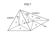
- FIG. 7 is a diagram for explaining intermediate magnetization of an anisotropy field.
- V i j is a certain area that is determined from an adjacent element and the center of gravity.
- Equation (18) represents two sets of intermediate magnetization m'(i,j) and m'(j,i) and Equations (19) to (22) represents an anisotropy field H an .
- the intermediate magnetization utilization unit 11 divides an element i into three elements V i j as illustrated in FIG. 7 and calculates an anisotropy field H an using intermediate magnetization corresponding to each element.
- the intermediate magnetization utilization unit 11 includes an intermediate magnetization calculation unit 21, an exchange field calculation unit 22, and an anisotropy field calculation unit 23.
- the intermediate magnetization calculation unit 21 calculates intermediate magnetization.
- the exchange field calculation unit 22 calculates an exchange field using the intermediate magnetization calculated by the intermediate magnetization calculation unit 21.
- the anisotropy field calculation unit 23 calculates an anisotropy field using the intermediate magnetization calculated by the intermediate magnetization calculation unit 21.
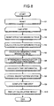
- FIG. 8 is a flowchart illustrating the flow of the magnetization analysis processing according to the embodiment. As illustrated in FIG. 8 , the magnetization analysis apparatus 1 first performs resetting for magnetization analysis (step S1).
- the magnetization analysis apparatus 1 then repeatedly performs the processing between step S2 and step S9 on all magnetization vectors m(i) for a given time at each time step.
- the effective magnetic field calculation unit 6 resets the effective magnetic field (step S3).
- the outer magnetic field calculation unit 9 calculates an outer magnetic field (step S4) and adds the outer magnetic field to the effective magnetic field.
- the demagnetizing field calculation unit 10 calculates a demagnetizing field (step S5) and adds the demagnetizing field to the effective magnetic field.
- the intermediate magnetization utilization unit 11 performs intermediate magnetization utilization processing of calculating an exchange field and an anisotropy field and adding the exchange field and the anisotropy field to the effective magnetic field (step S6).
- the magnetization calculation unit 7 calculates a time differential of a magnetization vector using the effective magnetic field (step S7) and updates the magnetization vector using the time differential of the magnetization vector (step S8).
- the result output unit 8 displays the calculation result (step S10). In other words, the result output unit 8 displays the result of simulating magnetization vectors on the display unit 3.
- FIG. 9 is a flowchart illustrating the flow of the intermediate magnetization utilization processing. As illustrated in FIG. 9 , the intermediate magnetization utilization unit 11 performs the processing between step S21 and step S29 as processing on an element i on all elements while changing i.
- the intermediate magnetization utilization unit 11 calculates a magnetization vector m(i) (step S22). As for each adjacent element j adjacent to an element i, the intermediate magnetization utilization unit 11 performs processing between step S23 and step S27.
- the intermediate magnetization calculation unit 21 performs intermediate magnetization with an adjacent element j (step S24).
- the exchange field calculation unit 22 then calculates an exchange field between elements i and j, i.e., an element i and an element j, and adds the exchange field to the exchange field of the element i (step S25).
- the anisotropy field calculation unit 23 then calculates an anisotropy field between the elements i and j and adds the anisotropy field to the anisotropy field of the element i (step S26).
- the intermediate magnetization utilization unit 11 adds the exchange field and the anisotropy field of the element i to the effective magnetic field of m(i) (step S28). Once the intermediate magnetization utilization unit 11 calculates an effective magnetic field as for each element i, the process ends (step S29).
- the intermediate magnetization utilization unit 11 calculates an exchange field and an an anisotropy field, which can improve the accuracy of calculating a magnetization vector.
- a pinning field H pin is an outer magnetic field at a time when an outer magnetic field is applied to a magnetic substance consisting of an A phase, a B phase, and a C phase and the domain near the B phase is withdrawn to the A phase.
- FIG. 10 is a diagram illustrating a domain wall pinning field calculation model. As illustrated in FIG. 10 , this model consists of three phases of an A phase, a B phase, and a C phase. The size of the B phase is 12 nm. The A, B, and C phases are different from one another in any one of parameters M s , K u , and A representing the magnetic properties of the magnetic material. When there is such spatial non-uniformity in the magnetic properties, domain wall pinning occurs.
- FIG. 11 is a diagram illustrating mesh-size dependency of a pinning field.
- the vertical axis represents H pin /H k and the horizontal axis represents the mesh interval, where H k is an anisotropy field (2K u /M s ).
- H k is an anisotropy field (2K u /M s ).
- the pinning field increases due to the numerical difference.
- the pinning filed is approximately the same as that of Theoretical solution (1), so that it is possible to calculate a pinning field highly accurately. This allows magnetization analysis apparatuses having the same specification to perform micromagnetic calculations in a much wider range.
- the intermediate magnetization calculation unit 21 calculates a magnetization vector at the halfway point between elements adjacent to each other as intermediate magnetization, and the exchange field calculation unit 22 and the anisotropy field calculation unit 23 calculate an exchange field and an anisotropy field, respectively, using the intermediate magnetization.
- the intermediate magnetization calculation unit 21 sets the magnitude of the magnetization vector of the intermediate magnetization at 1. Accordingly, the magnetization analysis apparatus 1 can calculate an exchange field and an anisotropy field accurately and calculate an effective magnetic field accurately. Thus, the magnetization analysis apparatus 1 can calculate magnetization vectors accurately, which improves the calculation accuracy of micromagnetic simulations.
- the magnetization analysis apparatus When simulations are performed with the halved mesh size, the magnetization analysis apparatus has to store the double amount of information at each dimension. On the other hand, when intermediate magnetization is used, it suffices if the magnetization analysis apparatus stores only information relevant to elements for which magnetization vectors are calculated, which allows a simulation with a smaller amount of memory than that in a case of the half mesh size.
- FIG. 12 is a diagram of an exemplary computer that executes the magnetization analysis program.
- a computer 200 includes a CPU 203 that executes various arithmetic operations, an input device 215 that receives input of data from a user, and a display control unit 207 that controls a display device 209.
- the computer 200 further includes a drive device 213 that reads a program, etc. from a storage medium and a communication control unit 217 that gives and receives data to and from other computers via a network.
- the computer 200 includes a memory 201 that temporarily stores various types of information and an HDD 205.
- the memory 201, the CPU 203, the HDD 205, the display control unit 207, the drive device 213, the input device 215, and the communication control unit 217 are connected via a bus 219.
- the drive device 213 is a device for, for example, a removable disk 211.
- the HDD 205 stores a magnetization analysis program 205a and magnetization analysis relevant information 205b.
- the CPU 203 reads and loads the magnetization analysis program 205a into a memory 201 and executes the magnetization analysis program 205a as a process.
- the magnetization analysis relevant information 205b corresponds to, for example, the mesh data 41, calculation condition data 42, and result data 43.
- the removable disk 211 stores each type of information, such as the magnetization analysis program 205a.
- the magnetization analysis program 205a is not necessarily stored in the HDD 205 in advance.
- the magnetization analysis program 205a may be stored in a "portable physical medium", such as a flexible disk (FD), a CD-ROM, a DVD disk, magneto-optical disk, or an IC card, that is inserted into the computer 200 and the computer 200 may read the magnetization analysis program 205a from the portable physical disk and execute the program.
- a "portable physical medium” such as a flexible disk (FD), a CD-ROM, a DVD disk, magneto-optical disk, or an IC card
Landscapes
- Physics & Mathematics (AREA)
- General Physics & Mathematics (AREA)
- Engineering & Computer Science (AREA)
- Condensed Matter Physics & Semiconductors (AREA)
- Theoretical Computer Science (AREA)
- General Engineering & Computer Science (AREA)
- Geometry (AREA)
- Evolutionary Computation (AREA)
- Computer Hardware Design (AREA)
- Measuring Magnetic Variables (AREA)
- Data Mining & Analysis (AREA)
- Mathematical Physics (AREA)
- Algebra (AREA)
- Computational Mathematics (AREA)
- Mathematical Analysis (AREA)
- Mathematical Optimization (AREA)
- Pure & Applied Mathematics (AREA)
- Databases & Information Systems (AREA)
- Software Systems (AREA)
Abstract
Description
- The embodiments discussed herein are related to a magnetization analysis apparatus, a magnetization analysis method, and a computer-readable recording medium.
- Micromagnetic simulation in which a magnetic substance is modeled as an assembly of small magnets and the domain state is numerically simulated is known as a technology for analyzing the magnetization behavior of a magnetic substance. Micromagnetic simulation is used to analyze the domain state of a micromagnetic device, such as a magnetic head of a hard disk drive (HDD) or a magnetoresistive random access memory (MRAM), and a magnetic material, such as a permanent magnet or a magnetic steel sheet.
-
FIG. 13 is a diagram for explaining modeling of a magnetic substance by micromagnetization. The micromagnetization refers to individual small magnets. As illustrated inFIG. 13 , amagnetic vector 92 is calculated permicromagnetization 91 in micromagnetic simulation. - In micromagnetic simulation, in order to ensure the calculation accuracy, the mesh size is adjusted such that the angles formed by magnetization vectors of meshes adjacent to each other are small angles so that the magnetization directions are regarded as approximately continuous. The mesh size is requested to be smaller than an exchange length. Particularly, in domain analysis on a permanent magnet with great magnetic anisotropy, the exchange length decreases to approximately one nanometer (nm). The exchange length represents the diameter of a crystal grain where an exchange occurs.
- When calculations are performed according to the tissue structure of a permanent magnet, because the permanent magnet has a crystal grain size of few micrometers (µm), the number of meshes increases with a mesh size of approximately 1 nm. If the mesh size is increased, flexibility used for calculations lowers, which can shorten the calculation time; however, because the angles formed by magnetization vectors adjacent to each other increase, the calculation accuracy significantly worsens. For this reason, if the mesh size is increased without consideration, the calculation accuracy is not ensured.
- Thus, there is a related technology in which the angle of rotation between two magnetization vectors arranged at the centers of elements (meshes) adjacent to each other is interpolated with reference to the rotation axis perpendicular to the two magnetization vectors and an exchange field is calculated.
- There is another related technology in which an effective magnetic field that acts on each element to be analyzed is calculated using, as a fixed value, a magnetic field calculated by magnetic field analysis using a finite element method and a magnetization vector in each element is calculated using the calculated effective magnetic field, so that the speed of analyzing the characteristics of a magnetic substance is increased.
- There is still another related technology in which a magnetic substance is divided into an analysis region and a non-analysis region and the non-analysis region is coarse grained using a representative region, so that the time for calculating the demagnetizing field from the non-analysis region acting on the magnetization in the analysis region and the calculation resources are reduced.
- Patent Document 1: Japanese Laid-open Patent Publication No.
2012-033116 - Patent Document 2: Japanese Laid-open Patent Publication No.
2013-131072 - Patent Document 3: Japanese Laid-open Patent Publication No.
2013-196462 - Micromagnetic simulation has a problem in that an increase in the mesh size worsens the calculation accuracy. For this reason, a technology that allows accurate simulations even with a mesh size that worsens the calculation accuracy is important.
- Accordingly, it is desirable to provide the calculation accuracy of micromagnetic simulation.
- According to an aspect of the embodiments, a magnetization analysis apparatus includes: an intermediate magnetization calculation unit that calculates, using a magnetization vector of each of elements obtained by mesh division in which a magnetic substance is divided into a plurality of meshes and a magnetization vector of an element adjacent to each element, intermediate magnetization that is a magnetization vector at the halfway point between each element and an element adjacent to each element; an effective magnetic field calculation unit that calculates an effective magnetic field using the intermediate magnetization calculated by the intermediate magnetization calculation unit; and a magnetization calculation unit that calculates a magnetization vector of each element after a unit time based on the effective magnetic field calculated by the effective magnetic field calculation unit.
-
-
FIG. 1 is a functional block diagram illustrating a configuration of a magnetization analysis apparatus according to an embodiment; -
FIG. 2 is a diagram illustrating a one-dimensional magnetization arrangement; -
FIG. 3 is a diagram illustrating a one-dimensional intermediate magnetization arrangement; -
FIG. 4 is a schematic diagram of two-dimensionally distributed discrete elements and magnetization; -
FIG. 5 is a diagram for explaining an adjacent-elements centroid distance vector and a normal vector at a side shared with an adjacent element; -
FIG. 6 is a diagram for explaining intermediate magnetization of an exchange field; -
FIG. 7 is a diagram for explaining intermediate magnetization of an anisotropy field; -
FIG. 8 is a flowchart illustrating a flow of magnetization analysis processing according to the embodiment; -
FIG. 9 is a flowchart illustrating a flow of intermediate magnetization utilization processing; -
FIG. 10 is a diagram illustrating a domain wall pinning field calculation model; -
FIG. 11 is a diagram illustrating mesh-size dependency of a pinning field; -
FIG. 12 is a diagram illustrating an exemplary computer that executes a magnetization analysis program; and -
FIG. 13 is a diagram for explaining modeling of a magnetic substance by micromagnetization. - Preferred embodiments will be explained, by way of example only, with reference to accompanying drawings. The magnetization analysis apparatus is an apparatus that performs micromagnetic simulations and that calculates a magnetization vector for a given time at each given time step and displays the magnetization vector. The present invention is not limited to the embodiment and it can be widely applied to magnetization analysis.
-
FIG. 1 is a functional block diagram illustrating a configuration of a magnetization analysis apparatus according to the embodiment. As illustrated inFIG. 1 , amagnetization apparatus 1 includes aninput unit 2, adisplay unit 3, astorage unit 4, and acontrol unit 5. - The
input unit 2 is an input device for a user who performs an analysis to input various types of information and instructions to themagnetization analysis apparatus 1. For example, theinput unit 2 corresponds to a keyboard, a mouse, and a touch panel. Thedisplay unit 3 is a display device that displays various types of information. For example, thedisplay unit 3 corresponds to a display. - The
storage unit 4 is a semiconductor memory device, such as a random access memory (RAM) or a flash memory, or a storage device, such as a hard disk or an optical disk. Thestorage unit 4stores mesh data 41,calculation condition data 42, and resultdata 43. - The
mesh data 41 is data consisting of a plurality of elements obtained by dividing a region of a magnetic substance to be analyzed into a finite number of regions by a finite element method or a finite difference method. An element is a region of a minimum unit that is obtained by dividing the region to be analyzed and consists of a plurality of nodes. - The
calculation condition data 42 is data on calculation conditions for magnetization analysis. Thecalculation condition data 42 contains, for example, the number of individual elements of meshes that are dealt with by a finite element method or a finite difference method and the value of a time step. - The
result data 43 is data illustrating the result of magnetization analysis, i.e., micromagnetic simulation. Theresult data 43 contains the value of calculation of a magnetic vector of each element for a given time at each time step. - The
control unit 5 corresponds to an electronic circuit, such as a central processing unit (CPU). Thecontrol unit 5 includes an internal memory for storing programs defining various processing procedures and control data and executes various types of processing according to the programs and control data. For example, thecontrol unit 5 executes magnetization analysis processing. In the magnetization analysis processing, themesh data 41 and thecalculation condition data 42 are read from thestorage unit 4 and calculations are started. In the magnetization analysis processing, during the calculation process, magnetization vectors are arranged at respective elements of themesh data 41 and the arranged magnetization vectors are saved as data at spots (e.g. magnetic fields) in thestorage unit 4. - The
control unit 5 includes an effective magneticfield calculation unit 6, amagnetization calculation unit 7, and aresult output unit 8. The effective magneticfield calculation unit 6 calculates an effective magnetic field of each element at each time step. Themagnetization calculation unit 7 calculates a magnetization vector at each time step from the effective magnetic field that is calculated by the effective magneticfield calculation unit 6 and stores the calculation result asresult data 42 in thestorage unit 4. Using theresult data 42, theresult output unit 8 outputs the magnetization vector for a given time to thedisplay unit 3. - The method of calculating a magnetization vector and an effective magnetic field will be described here. Equation (1) is an equation (control equation) that controls the motion of micromagnetization and that is referred to as the Landau-Lifshitz-Gilbert equation.

- In Equation (1), m added with "→" above its top, y, α, and Heff added with "→" above its top are a magnetization vector, a gyromagnetic ratio, a coefficient of friction, and an effective magnetic field, respectively. "→" denotes a vector. Hereinafter, "→" denoting a vector is used in only equations and will be omitted in other descriptions. "x" represents a cross product.
- As represented by Equation (2), the effective magnetic field Heff is a synthesis of a plurality of magnetic field vectors. The magnetic fields acting on the micro magnetization are an outer magnetic field Hout, a demagnetizing field Hdemag, an anisotropy field Han, and an exchange field Hex. Each of the demagnetizing field Hdemag, the anisotropy field Han, and the exchange field Hex are calculated according to Equations (3), (4) and (5), respectively.


- In the equations, φ is a magnetostatic potential, Ms is saturation magnetization, Ku is a magnetic anisotropy constant, uani is a magnetic anisotropy vector, and A is an exchange constant. The exchange field Hex is a force acting between atoms that are originally adjacent to each other. In order to perform an analysis while maintaining the calculation accuracy using an analysis model that is generated using mesh division that is division into a plurality of meshes each in a size larger than the distance between atoms, it is preferable to perform mesh division such that the change between the angles of magnetization vectors adjacent to each other is kept small to some extent.
- The following descriptions refer back to
FIG. 1 . The effective magneticfield calculation unit 6 includes an outer magneticfield calculation unit 9, a demagnetizingfield calculation unit 10, and an intermediatemagnetization utilization unit 11. The outer magneticfield calculation unit 9 calculates an outer magnetic field Hout at each time step. The demagnetizingfield calculation unit 10 calculates a demagnetizing field Hdemag at each time step. - The intermediate
magnetization utilization unit 11 calculates an anisotropy field Han and an exchange field Hex using intermediate magnetization. The intermediate magnetization is virtual magnetization that is arranged at the halfway point between sets of magnetization adjacent to each other. The magnitude of the magnetization vector of the intermediate magnetization is 1.FIG. 2 is a diagram illustrating a one-dimensional magnetization arrangement andFIG. 3 is a diagram illustrating a one-dimensional intermediate magnetization arrangement. - It is supposed that, as illustrated in
FIG. 2 , there is spatially discrete magnetization. According toFIG. 2 , magnetization in an area from a coordinate xn(i) to a coordinate xn(i+1) is denoted as a magnetization vector m(i), and m(i) is arranged at a center positon x(i) of the interval. In a normal one-dimensional finite volume method, an exchange field Hex and an anisotropy field Han are calculated according to the following Equations (6) and (7).

- On the other hand, the intermediate
magnetization utilization unit 11 arranges intermediate magnetization as illustrated inFIG. 3 . For example, the intermediatemagnetization utilization unit 11 arranges intermediate magnetization m'(i-1/2) at a center position xn(i) between x(i-1) and x(i) and arranges intermediate magnetization m'(i+1/2) at a center position xn(i+1) between x(i) and x(i+1). Equation (8) represents the intermediate magnetization and Equation (9) represents the coordinate of the position of the intermediate magnetization.

- The intermediate
magnetization utilization unit 11 calculates an exchange field Hex using the intermediate magnetization according to Equation (10) and calculate an anisotropy field Han according to Equations (11) to (13).
Equation 11


-
FIG. 4 is a schematic diagram of two-dimensionally distributed discrete elements and magnetization. It is supposed that, as illustrated inFIG. 4 , there is spatially discrete magnetization. According toFIG. 4 , a two-dimensional space is divided into triangular elements and the magnetization on each triangular element i is m(i) and m(i) is arranged at the center of gravity of each element. In a normal two-dimensional finite volume method, an exchange field Hex and anisotropy field Han are calculated according to the following Equations (14) and (15).

- In those equations, Vi is the area of a triangular element i and Sij is the length of a side shared between an element i and its adjacent element j, and l(i,j) and n(i,j) are an adjacent-elements centroid distance vector and a normal vector at a side shared with the adjacent element.
-
FIG. 5 is a diagram for explaining an adjacent-elements centroid distance vector and a normal vector at a side shared with an adjacent element. As illustrated inFIG. 5 , an adjacent-elements centroid distance vector l(i,j) is a vector from the center of gravity gi of an element i and toward the center of gravity gj of an element j. A normal vector n(i,j) at a side shared with the adjacent element is a vector from a side s shared with the adjacent element and toward the center of gravity gj of the element j, which is a vector perpendicular to the shared side s. In other words, the adjacent-elements centroid distance vector and the normal vector at the side shared with the adjacent element are toward the adjacent element. - On the other hand, the intermediate
magnetization utilization unit 11 calculates an exchange field and an anisotropy field.FIG. 6 is a diagram for explaining intermediate magnetization of an exchange field. Equation (16) represents intermediate magnetization m'(i,j) and Equation (17) represents an exchange field Hex.

- In the equations, l0(i,j) is, as illustrated in
FIG. 6 , a vector parallel to the vector of an adjacent element, connecting to the intersection with the shared side, and toward the adjacent element. -
FIG. 7 is a diagram for explaining intermediate magnetization of an anisotropy field. Vi j is a certain area that is determined from an adjacent element and the center of gravity. Equation (18) represents two sets of intermediate magnetization m'(i,j) and m'(j,i) and Equations (19) to (22) represents an anisotropy field Han. When calculating an anisotropy field, because an anisotropy field is formulated as a differential of energy per element volume, the intermediatemagnetization utilization unit 11 divides an element i into three elements Vi j as illustrated inFIG. 7 and calculates an anisotropy field Han using intermediate magnetization corresponding to each element.


- The following descriptions refer back to
FIG. 1 . The intermediatemagnetization utilization unit 11 includes an intermediatemagnetization calculation unit 21, an exchangefield calculation unit 22, and an anisotropyfield calculation unit 23. The intermediatemagnetization calculation unit 21 calculates intermediate magnetization. The exchangefield calculation unit 22 calculates an exchange field using the intermediate magnetization calculated by the intermediatemagnetization calculation unit 21. The anisotropyfield calculation unit 23 calculates an anisotropy field using the intermediate magnetization calculated by the intermediatemagnetization calculation unit 21. - The flow of the magnetization analysis processing according to the embodiment will be described here.
FIG. 8 is a flowchart illustrating the flow of the magnetization analysis processing according to the embodiment. As illustrated inFIG. 8 , themagnetization analysis apparatus 1 first performs resetting for magnetization analysis (step S1). - The
magnetization analysis apparatus 1 then repeatedly performs the processing between step S2 and step S9 on all magnetization vectors m(i) for a given time at each time step. Specifically, the effective magneticfield calculation unit 6 resets the effective magnetic field (step S3). The outer magneticfield calculation unit 9 calculates an outer magnetic field (step S4) and adds the outer magnetic field to the effective magnetic field. The demagnetizingfield calculation unit 10 calculates a demagnetizing field (step S5) and adds the demagnetizing field to the effective magnetic field. The intermediatemagnetization utilization unit 11 performs intermediate magnetization utilization processing of calculating an exchange field and an anisotropy field and adding the exchange field and the anisotropy field to the effective magnetic field (step S6). Themagnetization calculation unit 7 calculates a time differential of a magnetization vector using the effective magnetic field (step S7) and updates the magnetization vector using the time differential of the magnetization vector (step S8). - When the repetition for the given time completes, the
result output unit 8 displays the calculation result (step S10). In other words, theresult output unit 8 displays the result of simulating magnetization vectors on thedisplay unit 3. -
FIG. 9 is a flowchart illustrating the flow of the intermediate magnetization utilization processing. As illustrated inFIG. 9 , the intermediatemagnetization utilization unit 11 performs the processing between step S21 and step S29 as processing on an element i on all elements while changing i. - As for each element i, the intermediate
magnetization utilization unit 11 calculates a magnetization vector m(i) (step S22). As for each adjacent element j adjacent to an element i, the intermediatemagnetization utilization unit 11 performs processing between step S23 and step S27. - As for each adjacent element j, the intermediate
magnetization calculation unit 21 performs intermediate magnetization with an adjacent element j (step S24). The exchangefield calculation unit 22 then calculates an exchange field between elements i and j, i.e., an element i and an element j, and adds the exchange field to the exchange field of the element i (step S25). The anisotropyfield calculation unit 23 then calculates an anisotropy field between the elements i and j and adds the anisotropy field to the anisotropy field of the element i (step S26). - When the processing on all adjacent elements j completes, the intermediate
magnetization utilization unit 11 adds the exchange field and the anisotropy field of the element i to the effective magnetic field of m(i) (step S28). Once the intermediatemagnetization utilization unit 11 calculates an effective magnetic field as for each element i, the process ends (step S29). - As described above, the intermediate
magnetization utilization unit 11 calculates an exchange field and an an anisotropy field, which can improve the accuracy of calculating a magnetization vector. - In order to indicate the advantage of the embodiment, the mesh-size dependency of a domain wall pinning field of a material with great magnetic anisotropy will be described here. A pinning field Hpin is an outer magnetic field at a time when an outer magnetic field is applied to a magnetic substance consisting of an A phase, a B phase, and a C phase and the domain near the B phase is withdrawn to the A phase.
-
FIG. 10 is a diagram illustrating a domain wall pinning field calculation model. As illustrated inFIG. 10 , this model consists of three phases of an A phase, a B phase, and a C phase. The size of the B phase is 12 nm. The A, B, and C phases are different from one another in any one of parameters Ms, Ku, and A representing the magnetic properties of the magnetic material. When there is such spatial non-uniformity in the magnetic properties, domain wall pinning occurs. -
FIG. 11 is a diagram illustrating mesh-size dependency of a pinning field. InFIG. 11 , the vertical axis represents Hpin/Hk and the horizontal axis represents the mesh interval, where Hk is an anisotropy field (2Ku/Ms). As illustrated inFIG. 11 , in Related method (2), when the mesh interval increases, the pinning field increases due to the numerical difference. On the other hand, in the case of (3) where the intermediate magnetization according to the embodiment is used, even when the mesh interval is increased to approximately 2 nm, the pinning filed is approximately the same as that of Theoretical solution (1), so that it is possible to calculate a pinning field highly accurately. This allows magnetization analysis apparatuses having the same specification to perform micromagnetic calculations in a much wider range. - As described above, according to the embodiment, the intermediate
magnetization calculation unit 21 calculates a magnetization vector at the halfway point between elements adjacent to each other as intermediate magnetization, and the exchangefield calculation unit 22 and the anisotropyfield calculation unit 23 calculate an exchange field and an anisotropy field, respectively, using the intermediate magnetization. The intermediatemagnetization calculation unit 21 sets the magnitude of the magnetization vector of the intermediate magnetization at 1. Accordingly, themagnetization analysis apparatus 1 can calculate an exchange field and an anisotropy field accurately and calculate an effective magnetic field accurately. Thus, themagnetization analysis apparatus 1 can calculate magnetization vectors accurately, which improves the calculation accuracy of micromagnetic simulations. - When simulations are performed with the halved mesh size, the magnetization analysis apparatus has to store the double amount of information at each dimension. On the other hand, when intermediate magnetization is used, it suffices if the magnetization analysis apparatus stores only information relevant to elements for which magnetization vectors are calculated, which allows a simulation with a smaller amount of memory than that in a case of the half mesh size.
- Various types of processing described in the embodiment can be implemented by executing a program prepared in advance by a computer, such as a personal computer or a work station. An exemplary computer that executes a magnetic analysis program that implements the same functions as those of the
magnetization analysis apparatus 1 illustrated inFIG. 1 will be described below.FIG. 12 is a diagram of an exemplary computer that executes the magnetization analysis program. - As illustrated in
FIG. 12 , acomputer 200 includes aCPU 203 that executes various arithmetic operations, aninput device 215 that receives input of data from a user, and adisplay control unit 207 that controls adisplay device 209. Thecomputer 200 further includes adrive device 213 that reads a program, etc. from a storage medium and acommunication control unit 217 that gives and receives data to and from other computers via a network. Thecomputer 200 includes amemory 201 that temporarily stores various types of information and anHDD 205. Thememory 201, theCPU 203, theHDD 205, thedisplay control unit 207, thedrive device 213, theinput device 215, and thecommunication control unit 217 are connected via abus 219. - The
drive device 213 is a device for, for example, aremovable disk 211. TheHDD 205 stores amagnetization analysis program 205a and magnetization analysisrelevant information 205b. - The
CPU 203 reads and loads themagnetization analysis program 205a into amemory 201 and executes themagnetization analysis program 205a as a process. The magnetization analysisrelevant information 205b corresponds to, for example, themesh data 41,calculation condition data 42, and resultdata 43. For example, theremovable disk 211 stores each type of information, such as themagnetization analysis program 205a. - The
magnetization analysis program 205a is not necessarily stored in theHDD 205 in advance. For example, themagnetization analysis program 205a may be stored in a "portable physical medium", such as a flexible disk (FD), a CD-ROM, a DVD disk, magneto-optical disk, or an IC card, that is inserted into thecomputer 200 and thecomputer 200 may read themagnetization analysis program 205a from the portable physical disk and execute the program. - As the embodiment, a case where an exchange field and an anisotropy field using intermediate magnetization has been described; however, the present invention is not limited to this. The present invention can be applied to, for example, a case where only an exchange filed or an anisotropy field is calculated using intermediate magnetization.
- According to the embodiment, it is possible to improve the calculation accuracy of micromagnetic simulations.
Claims (6)
- A magnetization analysis apparatus (1) comprising:an intermediate magnetization calculation unit (21) configured to calculate, using a magnetization vector of each of elements obtained by mesh division in which a magnetic substance is divided into a plurality of meshes and a magnetization vector of an element adjacent to each element, intermediate magnetization that is a magnetization vector at the halfway point between each element and an element adjacent to each element;an effective magnetic field calculation unit (6) configured to calculate an effective magnetic field using the intermediate magnetization calculated by the intermediate magnetization calculation unit; anda magnetization calculation unit (7) configured to calculate a magnetization vector of each element after a unit time based on the effective magnetic field calculated by the effective magnetic field calculation unit.
- The magnetization analysis apparatus (1) according to claim 1, wherein the effective magnetic field calculation unit (6) is configured to calculate an effective magnetic field by calculating an exchange field and an anisotropy field using the intermediate magnetization.
- The magnetization analysis apparatus (1) according to claim 1 or 2, wherein the intermediate magnetization calculation unit (21) is configured to calculate intermediate magnetization including a magnitude of 1.
- The magnetization analysis apparatus (1) according to claim 2, wherein
the intermediate magnetization calculation unit (21) is configured to calculate, in a case of two dimensions, two sets of intermediate magnetization to calculate the anisotropy field, and
the effective magnetic field calculation unit (6) is configured to calculate the anisotropy field using the two sets of intermediate magnetization. - A magnetization analysis method for a computer (200) to execute a process comprising:first calculating, using a magnetization vector of each of elements obtained by mesh division in which a magnetic substance is divided into a plurality of meshes and a magnetization vector of an element adjacent to each element, intermediate magnetization that is a magnetization vector at the halfway point between each element and an element adjacent to each element;second calculating an effective magnetic field using the intermediate magnetization calculated at the first calculating; andthird calculating a magnetization vector of each element after a unit time based on the effective magnetic field calculated at the second calculating.
- A magnetization analysis program (205a) that causes a computer (200) to execute a process comprising:first calculating, using a magnetization vector of each of elements obtained by mesh division in which a magnetic substance is divided into a plurality of meshes and a magnetization vector of an element adjacent to each element, intermediate magnetization that is a magnetization vector at the halfway point between each element and an element adjacent to each element;second calculating an effective magnetic field using the intermediate magnetization calculated at the first calculating; andthird calculating a magnetization vector of each element after a unit time based on the effective magnetic field calculated at the second calculating.
Applications Claiming Priority (1)
| Application Number | Priority Date | Filing Date | Title |
|---|---|---|---|
| JP2014164980A JP6384189B2 (en) | 2014-08-13 | 2014-08-13 | Magnetization analysis apparatus, magnetization analysis method, and magnetization analysis program |
Publications (1)
| Publication Number | Publication Date |
|---|---|
| EP3040887A1 true EP3040887A1 (en) | 2016-07-06 |
Family
ID=53434244
Family Applications (1)
| Application Number | Title | Priority Date | Filing Date |
|---|---|---|---|
| EP15172063.8A Withdrawn EP3040887A1 (en) | 2014-08-13 | 2015-06-15 | Magnetization analysis apparatus, magnetization analysis method, and magnetization analysis program |
Country Status (3)
| Country | Link |
|---|---|
| US (1) | US9824168B2 (en) |
| EP (1) | EP3040887A1 (en) |
| JP (1) | JP6384189B2 (en) |
Cited By (1)
| Publication number | Priority date | Publication date | Assignee | Title |
|---|---|---|---|---|
| CN106295036A (en) * | 2016-08-16 | 2017-01-04 | 京磁材料科技股份有限公司 | A kind of computational methods of neodymium iron boron magnetic body anisotropy field |
Families Citing this family (2)
| Publication number | Priority date | Publication date | Assignee | Title |
|---|---|---|---|---|
| JP7053999B2 (en) * | 2018-06-12 | 2022-04-13 | 富士通株式会社 | Information processing device, closed magnetic path calculation method, and closed magnetic path calculation system |
| CN114265122B (en) * | 2021-12-22 | 2024-12-03 | 中南大学 | A magnetic signal response analysis method and system based on an arbitrary polyhedron model of linear magnetization |
Citations (3)
| Publication number | Priority date | Publication date | Assignee | Title |
|---|---|---|---|---|
| US20120029849A1 (en) * | 2010-08-02 | 2012-02-02 | Fujitsu Limited | Magnetic exchange coupling energy calculating method and apparatus |
| JP2013131072A (en) | 2011-12-21 | 2013-07-04 | Fujitsu Ltd | Program, apparatus and method for magnetic body property analysis |
| JP2013196462A (en) | 2012-03-21 | 2013-09-30 | Hitachi Ltd | Magnetic characteristic calculation method, magnetization motion visualization device and program for the same |
Family Cites Families (7)
| Publication number | Priority date | Publication date | Assignee | Title |
|---|---|---|---|---|
| JPH10124479A (en) * | 1996-10-24 | 1998-05-15 | Sony Corp | Analysis method of magnetization distribution |
| US7868404B2 (en) * | 2007-11-01 | 2011-01-11 | Nve Corporation | Vortex spin momentum transfer magnetoresistive device |
| JP2010277654A (en) | 2009-05-29 | 2010-12-09 | Fuji Electric Device Technology Co Ltd | Accelerated simulation method for thermal relaxation process of magnetization |
| EP2549396A4 (en) * | 2010-03-18 | 2017-12-06 | Fujitsu Limited | Method for simulating magnetic material, and program |
| US8849627B2 (en) * | 2010-07-19 | 2014-09-30 | Terje Graham Vold | Computer simulation of electromagnetic fields |
| JP5589665B2 (en) * | 2010-08-18 | 2014-09-17 | 富士通株式会社 | Analysis device, analysis program, and analysis method |
| JP6221688B2 (en) * | 2013-11-27 | 2017-11-01 | 富士通株式会社 | Magnetic body analysis apparatus, magnetic body analysis program, and magnetic body analysis method |
-
2014
- 2014-08-13 JP JP2014164980A patent/JP6384189B2/en active Active
-
2015
- 2015-06-12 US US14/737,537 patent/US9824168B2/en active Active
- 2015-06-15 EP EP15172063.8A patent/EP3040887A1/en not_active Withdrawn
Patent Citations (4)
| Publication number | Priority date | Publication date | Assignee | Title |
|---|---|---|---|---|
| US20120029849A1 (en) * | 2010-08-02 | 2012-02-02 | Fujitsu Limited | Magnetic exchange coupling energy calculating method and apparatus |
| JP2012033116A (en) | 2010-08-02 | 2012-02-16 | Fujitsu Ltd | Calculation program, calculation method and calculation apparatus of magnetic exchange coupling energy |
| JP2013131072A (en) | 2011-12-21 | 2013-07-04 | Fujitsu Ltd | Program, apparatus and method for magnetic body property analysis |
| JP2013196462A (en) | 2012-03-21 | 2013-09-30 | Hitachi Ltd | Magnetic characteristic calculation method, magnetization motion visualization device and program for the same |
Non-Patent Citations (2)
| Title |
|---|
| BOTTAUSCIO O ET AL: "A Finite Element Procedure for Dynamic Micromagnetic Computations", IEEE TRANSACTIONS ON MAGNETICS, IEEE SERVICE CENTER, NEW YORK, NY, US, vol. 44, no. 11, 1 November 2008 (2008-11-01), pages 3149 - 3152, XP011240034, ISSN: 0018-9464, DOI: 10.1109/TMAG.2008.2001666 * |
| LOPEZ-DIAZ L ET AL: "Topical Review;Micromagnetic simulations using Graphics Processing Units;Micromagnetic simulations using Graphics Processing Units", JOURNAL OF PHYSICS D: APPLIED PHYSICS, INSTITUTE OF PHYSICS PUBLISHING LTD, GB, vol. 45, no. 32, 27 July 2012 (2012-07-27), pages 323001, XP020226739, ISSN: 0022-3727, DOI: 10.1088/0022-3727/45/32/323001 * |
Cited By (2)
| Publication number | Priority date | Publication date | Assignee | Title |
|---|---|---|---|---|
| CN106295036A (en) * | 2016-08-16 | 2017-01-04 | 京磁材料科技股份有限公司 | A kind of computational methods of neodymium iron boron magnetic body anisotropy field |
| CN106295036B (en) * | 2016-08-16 | 2019-08-02 | 京磁材料科技股份有限公司 | A kind of calculation method of neodymium iron boron magnetic body anisotropy field |
Also Published As
| Publication number | Publication date |
|---|---|
| US20160048617A1 (en) | 2016-02-18 |
| JP2016042216A (en) | 2016-03-31 |
| JP6384189B2 (en) | 2018-09-05 |
| US9824168B2 (en) | 2017-11-21 |
Similar Documents
| Publication | Publication Date | Title |
|---|---|---|
| Lee et al. | Vibrations of Timoshenko beams with isogeometric approach | |
| Guo et al. | On solving the 3-D phase field equations by employing a parallel-adaptive mesh refinement (Para-AMR) algorithm | |
| Beleggia et al. | On the computation of the demagnetization tensor field for an arbitrary particle shape using a Fourier space approach | |
| Chang et al. | FastMag: Fast micromagnetic simulator for complex magnetic structures | |
| Wu et al. | Statistical moving load identification including uncertainty | |
| Katz et al. | High aspect ratio grid effects on the accuracy of Navier–Stokes solutions on unstructured meshes | |
| JP5785533B2 (en) | Brain current calculation method, calculation device, and computer program | |
| EP2607913A2 (en) | Magnetic property analyzing method and apparatus | |
| EP2416169B1 (en) | Magnetic exchange coupling energy calculating method and apparatus | |
| US9117041B2 (en) | Magnetic property analyzing apparatus and method | |
| EP2270694A2 (en) | Magnetic-field analyzing apparatus and magnetic-field analyzing program | |
| EP3040887A1 (en) | Magnetization analysis apparatus, magnetization analysis method, and magnetization analysis program | |
| Kim et al. | Numerical study of viscosity and inertial effects on tank-treading and tumbling motions of vesicles under shear flow | |
| Rhee et al. | Dislocation stress fields for dynamic codes using anisotropic elasticity: methodology and analysis | |
| KR20140110336A (en) | Semiconductor device simulation system and method for simulating semiconductor device using it | |
| Gerrits et al. | Towards Glyphs for Uncertain Symmetric Second‐Order Tensors | |
| Bottauscio et al. | Parallelized micromagnetic solver for the efficient simulation of large patterned magnetic nanostructures | |
| JP6015761B2 (en) | Magnetic body simulation program, simulation apparatus, and simulation method | |
| Spillmann et al. | Inextensible elastic rods with torsional friction based on Lagrange multipliers | |
| US20170068762A1 (en) | Simulation device, simulation program, and simulation method | |
| JP6065616B2 (en) | Simulation program, simulation method, and simulation apparatus | |
| JP2021110997A (en) | Simulation method, simulation device, and program | |
| JP6891613B2 (en) | Magnetic material simulation program, magnetic material simulation device, and magnetic material simulation method | |
| JP6540193B2 (en) | INFORMATION PROCESSING APPARATUS, PROGRAM, AND INFORMATION PROCESSING METHOD | |
| Manzin et al. | A 2.5 D micromagnetic solver for randomly distributed magnetic thin objects |
Legal Events
| Date | Code | Title | Description |
|---|---|---|---|
| PUAI | Public reference made under article 153(3) epc to a published international application that has entered the european phase |
Free format text: ORIGINAL CODE: 0009012 |
|
| AK | Designated contracting states |
Kind code of ref document: A1 Designated state(s): AL AT BE BG CH CY CZ DE DK EE ES FI FR GB GR HR HU IE IS IT LI LT LU LV MC MK MT NL NO PL PT RO RS SE SI SK SM TR |
|
| AX | Request for extension of the european patent |
Extension state: BA ME |
|
| 17P | Request for examination filed |
Effective date: 20161010 |
|
| RBV | Designated contracting states (corrected) |
Designated state(s): AL AT BE BG CH CY CZ DE DK EE ES FI FR GB GR HR HU IE IS IT LI LT LU LV MC MK MT NL NO PL PT RO RS SE SI SK SM TR |
|
| STAA | Information on the status of an ep patent application or granted ep patent |
Free format text: STATUS: THE APPLICATION HAS BEEN WITHDRAWN |
|
| 18W | Application withdrawn |
Effective date: 20171030 |