EP2867894B1 - Device, method and computer program for freely selectable frequency shifts in the sub-band domain - Google Patents
Device, method and computer program for freely selectable frequency shifts in the sub-band domain Download PDFInfo
- Publication number
- EP2867894B1 EP2867894B1 EP13737170.4A EP13737170A EP2867894B1 EP 2867894 B1 EP2867894 B1 EP 2867894B1 EP 13737170 A EP13737170 A EP 13737170A EP 2867894 B1 EP2867894 B1 EP 2867894B1
- Authority
- EP
- European Patent Office
- Prior art keywords
- frequency
- coefficients
- mdct
- subband
- signal
- Prior art date
- Legal status (The legal status is an assumption and is not a legal conclusion. Google has not performed a legal analysis and makes no representation as to the accuracy of the status listed.)
- Active
Links
- 238000000034 method Methods 0.000 title claims description 133
- 238000004590 computer program Methods 0.000 title claims description 20
- 238000001228 spectrum Methods 0.000 claims description 127
- 239000011159 matrix material Substances 0.000 claims description 103
- 230000003595 spectral effect Effects 0.000 claims description 73
- 230000005236 sound signal Effects 0.000 claims description 59
- 238000001914 filtration Methods 0.000 claims description 25
- 230000002829 reductive effect Effects 0.000 claims description 17
- 230000001419 dependent effect Effects 0.000 claims description 16
- 230000006978 adaptation Effects 0.000 claims description 14
- 230000015572 biosynthetic process Effects 0.000 claims description 13
- 238000003786 synthesis reaction Methods 0.000 claims description 12
- 230000001131 transforming effect Effects 0.000 claims 2
- 230000009466 transformation Effects 0.000 description 115
- 230000006870 function Effects 0.000 description 53
- 230000004044 response Effects 0.000 description 33
- 238000004364 calculation method Methods 0.000 description 29
- 238000012545 processing Methods 0.000 description 27
- 230000008569 process Effects 0.000 description 25
- 238000004422 calculation algorithm Methods 0.000 description 21
- 238000007792 addition Methods 0.000 description 17
- 238000004458 analytical method Methods 0.000 description 14
- 238000000844 transformation Methods 0.000 description 14
- 239000013598 vector Substances 0.000 description 14
- 230000000873 masking effect Effects 0.000 description 13
- 230000010076 replication Effects 0.000 description 12
- 230000008901 benefit Effects 0.000 description 11
- 230000005540 biological transmission Effects 0.000 description 10
- 238000005457 optimization Methods 0.000 description 10
- 230000009467 reduction Effects 0.000 description 10
- 238000000354 decomposition reaction Methods 0.000 description 9
- 238000011156 evaluation Methods 0.000 description 9
- 238000013139 quantization Methods 0.000 description 9
- 238000005070 sampling Methods 0.000 description 9
- 238000012546 transfer Methods 0.000 description 9
- 238000010586 diagram Methods 0.000 description 8
- 230000002123 temporal effect Effects 0.000 description 8
- 238000005516 engineering process Methods 0.000 description 7
- 230000036961 partial effect Effects 0.000 description 7
- 230000000694 effects Effects 0.000 description 6
- 238000006243 chemical reaction Methods 0.000 description 5
- 238000007906 compression Methods 0.000 description 5
- 230000006835 compression Effects 0.000 description 5
- 238000009795 derivation Methods 0.000 description 5
- 230000002452 interceptive effect Effects 0.000 description 5
- 230000008447 perception Effects 0.000 description 5
- 238000013459 approach Methods 0.000 description 4
- 230000008859 change Effects 0.000 description 4
- 238000013144 data compression Methods 0.000 description 4
- 229910003460 diamond Inorganic materials 0.000 description 4
- 239000010432 diamond Substances 0.000 description 4
- 238000012986 modification Methods 0.000 description 4
- 230000004048 modification Effects 0.000 description 4
- 230000001629 suppression Effects 0.000 description 4
- 238000012360 testing method Methods 0.000 description 4
- OVOUKWFJRHALDD-UHFFFAOYSA-N 2-[2-(2-acetyloxyethoxy)ethoxy]ethyl acetate Chemical compound CC(=O)OCCOCCOCCOC(C)=O OVOUKWFJRHALDD-UHFFFAOYSA-N 0.000 description 3
- 238000001514 detection method Methods 0.000 description 3
- 238000011835 investigation Methods 0.000 description 3
- 239000000463 material Substances 0.000 description 3
- 230000010355 oscillation Effects 0.000 description 3
- 241000282412 Homo Species 0.000 description 2
- 230000003321 amplification Effects 0.000 description 2
- 210000000721 basilar membrane Anatomy 0.000 description 2
- 238000004891 communication Methods 0.000 description 2
- 125000004122 cyclic group Chemical group 0.000 description 2
- 230000006378 damage Effects 0.000 description 2
- 238000011161 development Methods 0.000 description 2
- 238000006073 displacement reaction Methods 0.000 description 2
- 238000003199 nucleic acid amplification method Methods 0.000 description 2
- 230000000737 periodic effect Effects 0.000 description 2
- 238000004321 preservation Methods 0.000 description 2
- 230000001052 transient effect Effects 0.000 description 2
- QDGIAPPCJRFVEK-UHFFFAOYSA-N (1-methylpiperidin-4-yl) 2,2-bis(4-chlorophenoxy)acetate Chemical compound C1CN(C)CCC1OC(=O)C(OC=1C=CC(Cl)=CC=1)OC1=CC=C(Cl)C=C1 QDGIAPPCJRFVEK-UHFFFAOYSA-N 0.000 description 1
- 101100171060 Caenorhabditis elegans div-1 gene Proteins 0.000 description 1
- 241000819038 Chichester Species 0.000 description 1
- 108010076504 Protein Sorting Signals Proteins 0.000 description 1
- 108010063499 Sigma Factor Proteins 0.000 description 1
- 230000003044 adaptive effect Effects 0.000 description 1
- 238000007630 basic procedure Methods 0.000 description 1
- 230000006399 behavior Effects 0.000 description 1
- 230000008033 biological extinction Effects 0.000 description 1
- 230000000903 blocking effect Effects 0.000 description 1
- 239000000872 buffer Substances 0.000 description 1
- 229910052799 carbon Inorganic materials 0.000 description 1
- 238000012512 characterization method Methods 0.000 description 1
- 239000012141 concentrate Substances 0.000 description 1
- 230000021615 conjugation Effects 0.000 description 1
- 230000001186 cumulative effect Effects 0.000 description 1
- 230000003247 decreasing effect Effects 0.000 description 1
- 230000003111 delayed effect Effects 0.000 description 1
- 238000013461 design Methods 0.000 description 1
- 230000003203 everyday effect Effects 0.000 description 1
- 238000002474 experimental method Methods 0.000 description 1
- 230000030279 gene silencing Effects 0.000 description 1
- 230000010354 integration Effects 0.000 description 1
- 230000002427 irreversible effect Effects 0.000 description 1
- 238000012423 maintenance Methods 0.000 description 1
- 238000010295 mobile communication Methods 0.000 description 1
- 238000010606 normalization Methods 0.000 description 1
- 230000003287 optical effect Effects 0.000 description 1
- 230000010363 phase shift Effects 0.000 description 1
- 238000011084 recovery Methods 0.000 description 1
- 238000009877 rendering Methods 0.000 description 1
- 230000000717 retained effect Effects 0.000 description 1
- 230000002441 reversible effect Effects 0.000 description 1
- 230000003068 static effect Effects 0.000 description 1
- 230000036962 time dependent Effects 0.000 description 1
- 230000007704 transition Effects 0.000 description 1
- 230000017105 transposition Effects 0.000 description 1
Images


Classifications
-
- G—PHYSICS
- G10—MUSICAL INSTRUMENTS; ACOUSTICS
- G10L—SPEECH ANALYSIS OR SYNTHESIS; SPEECH RECOGNITION; SPEECH OR VOICE PROCESSING; SPEECH OR AUDIO CODING OR DECODING
- G10L25/00—Speech or voice analysis techniques not restricted to a single one of groups G10L15/00 - G10L21/00
- G10L25/03—Speech or voice analysis techniques not restricted to a single one of groups G10L15/00 - G10L21/00 characterised by the type of extracted parameters
- G10L25/18—Speech or voice analysis techniques not restricted to a single one of groups G10L15/00 - G10L21/00 characterised by the type of extracted parameters the extracted parameters being spectral information of each sub-band
-
- G—PHYSICS
- G10—MUSICAL INSTRUMENTS; ACOUSTICS
- G10L—SPEECH ANALYSIS OR SYNTHESIS; SPEECH RECOGNITION; SPEECH OR VOICE PROCESSING; SPEECH OR AUDIO CODING OR DECODING
- G10L19/00—Speech or audio signals analysis-synthesis techniques for redundancy reduction, e.g. in vocoders; Coding or decoding of speech or audio signals, using source filter models or psychoacoustic analysis
- G10L19/02—Speech or audio signals analysis-synthesis techniques for redundancy reduction, e.g. in vocoders; Coding or decoding of speech or audio signals, using source filter models or psychoacoustic analysis using spectral analysis, e.g. transform vocoders or subband vocoders
-
- G—PHYSICS
- G10—MUSICAL INSTRUMENTS; ACOUSTICS
- G10L—SPEECH ANALYSIS OR SYNTHESIS; SPEECH RECOGNITION; SPEECH OR VOICE PROCESSING; SPEECH OR AUDIO CODING OR DECODING
- G10L21/00—Processing of the speech or voice signal to produce another audible or non-audible signal, e.g. visual or tactile, in order to modify its quality or its intelligibility
- G10L21/02—Speech enhancement, e.g. noise reduction or echo cancellation
- G10L21/038—Speech enhancement, e.g. noise reduction or echo cancellation using band spreading techniques
- G10L21/0388—Details of processing therefor
-
- H—ELECTRICITY
- H03—ELECTRONIC CIRCUITRY
- H03G—CONTROL OF AMPLIFICATION
- H03G3/00—Gain control in amplifiers or frequency changers without distortion of the input signal
-
- G—PHYSICS
- G10—MUSICAL INSTRUMENTS; ACOUSTICS
- G10L—SPEECH ANALYSIS OR SYNTHESIS; SPEECH RECOGNITION; SPEECH OR VOICE PROCESSING; SPEECH OR AUDIO CODING OR DECODING
- G10L19/00—Speech or audio signals analysis-synthesis techniques for redundancy reduction, e.g. in vocoders; Coding or decoding of speech or audio signals, using source filter models or psychoacoustic analysis
- G10L19/02—Speech or audio signals analysis-synthesis techniques for redundancy reduction, e.g. in vocoders; Coding or decoding of speech or audio signals, using source filter models or psychoacoustic analysis using spectral analysis, e.g. transform vocoders or subband vocoders
- G10L19/0204—Speech or audio signals analysis-synthesis techniques for redundancy reduction, e.g. in vocoders; Coding or decoding of speech or audio signals, using source filter models or psychoacoustic analysis using spectral analysis, e.g. transform vocoders or subband vocoders using subband decomposition
Definitions
- the present invention relates to audio signal processing and, more particularly, to an apparatus, method and computer program for arbitrary frequency shifts in the subband domain.
- Audio signal processing is becoming increasingly important.
- audio coders on the market, e.g. realized by algorithms for digital processing of audio material for storage or transmission.
- the goal of any encoding process is to compress the information content of a signal in such a way that it requires a minimum of storage space while maintaining the highest possible reproduction quality.
- the efficiency of modern audio coders depends primarily on the required storage space and, among other things, on the required calculation effort of the algorithm.
- a digital audio coder is in principle an instrument for transferring audio signals into a format suitable for storage or transmission. This happens on the transmitter side of the audio encoder (encoder). The data thus generated are then returned to their original form in the receiver (decoder) and ideally correspond to the original data except for a constant delay (English: Delay).
- the general goal of audio coders is to minimize the amount of data needed to represent the audio signal while maximizing perceived ones Playback quality.
- Developing an audio coder requires a number of factors such as fidelity, data rate, and complexity.
- the delay added by processing the signal also plays an important role (Bosi and Goldberg, 2003).
- Another aspect is the quality of the reproduced coded audio signals.
- Many audio coders reduce the amount of data via Irrelevanzredulement. In this case, signal components are lost depending on the data rate. At low data rates, this reduces the quality of reproduced audio signals.
- the lossless audio coding on the receiver side allows an exact reconstruction of the original signal.
- the lossy process via a model of subjective perception causes irreversible deviations from the original signal (Zölzer, 2005).
- the lossless audio coding is based on the reduction of the redundancy contained in the signal to be coded.
- One common method is, for example, Linear Predictive Coding (LPC) in conjunction with subsequent entropy coding.
- LPC Linear Predictive Coding
- Such audio coding methods allow bit-accurate reconstruction of the input signal from the coded bitstream.
- Linear prediction uses statistical dependencies between successive samples of the signal to predict future values. This is due to the fact that successive samples are more similar as more distant.
- the prediction is realized by a linear prediction filter which estimates the current sample by a series of previous samples. However, it is not this estimate itself that is processed further, but the difference between this value and the actual sample at this point.
- the goal of linear prediction is to minimize the energy of this error signal through optimized filters and to transmit this error signal, which requires only a small bandwidth (Weinzierl, 2008).
- the error signal is entropy coded.
- the entropy is a measure of the average information content of a signal and indicates the theoretical minimum of the bits required for the encoding.
- a typical method is the Huffman coding. In this case, individual sample values are assigned specific code words as a function of their statistical probability of occurrence. Frequently occurring samples are assigned short symbols and rarely occurring signal values are represented by long code words. On average, the coded signal is represented by the smallest possible number of bits (Bosi and Goldberg, 2003).
- Both the linear prediction and the entropy coding are reversible and thus remove no information from the signal. By combining both methods, only redundancies are removed from the signal to be coded. Since such lossless approaches depend strongly on the signal characteristic, the coding gain is comparatively low.
- the achieved compression rate ie the ratio of input bit rate and bit rate of the encoded signal, is in the range of 1.5: 1 to 3: 1 (Weinzierl, 2008).
- the lossy audio coding is based on the principle of irrelevance reduction. These methods require a model of human perception that describes psychoacoustic phenomena of hearing in terms of time and frequency resolution. Therefore, lossy audio coding is also referred to as perceptual or psychoacoustic coding. In the field of audio coding, all signal components that are not perceivable by humans and therefore inaudible are called irrelevant (Zölzer, 2005). In order to understand the functionality of a perception-adapted audio coder in more detail, a sound knowledge of psychoacoustics is of great importance.
- the human ear analyzes a sound event by breaking it up into frequency groups. These frequency groups are represented on the Bark scale and referred to in the English literature as Critical Bands. Each of these frequency groups combines a frequency range that is evaluated jointly by the ear. In this case, a frequency range corresponds to a local area on the Basilar membrane. A total of 24 critical bands are assigned to the basilar membrane, whose bandwidth increases with increasing frequency (Fastl and Zwicker, 2007). Lossy audio coders adopt this model of frequency groups to break broadband signals into subbands and code each band individually (Zölzer, 2005). Often, this model is adjusted and instead of the Bark scale a linear frequency distribution with more than 24 bands used.
- Another important feature of auditory perception is the frequency-dependent loudness perception of tones of the same sound pressure level. This results in two characteristics of the hearing. On the one hand, tones of different frequencies but with the same sound pressure level are perceived as having different loudnesses, on the other hand there is a frequency-dependent threshold from which sounds can still be perceived (Fastl and Zwicker, 2007). This threshold is also referred to as the absolute hearing threshold or rest hearing threshold and is in Fig. 22 shown. Two conclusions can be drawn for audio coding. Signals whose levels are below the absolute threshold of hearing, need not be processed, since they are not perceived anyway. In addition, the number of required quantization steps per frequency band can be determined from the distance between the quiet auditory threshold and the signal level (Zölzer, 2005).
- Fig. 21 shows a schematic representation of a temporal masking. Specially shows Fig. 21 schematically the areas of the pre- and Postmaskings and in each case the level under which signals are hidden. Temporal occlusion may be used in audio coding to reduce the noise produced by the encoding process, such as quantization noise from high level signal sequences To hide (transients).
- Fig. 22 shows a schematic representation of the frequency-dependent masking in human hearing. As can be seen, the masked sound lies below the masking threshold of the masker and is therefore inaudible. This effect is exploited in lossy audio coding. Signal components that lie below the frequency-dependent listening threshold are removed from the signal and not further processed (Zölzer, 2005).
- Fig. 23 The general structure of a typical perceptual encoder is in Fig. 23 shown. It shows Fig. 23 a block diagram of a psychoacoustic audio encoder.
- the PCM signal to be coded is split into frequency bands by the analysis filterbank and fed to the psychoacoustic model. Therein, a time-dependent listening threshold is determined by the described psychoacoustic properties of the hearing, which regulates the accuracy of the quantization for the different frequency bands.
- important, so well perceptible, frequency bands are quantized very high resolution and unimportant are displayed with a few bits of resolution.
- entropy coding is performed for data reduction.
- the bitstream multiplexer assembles the actual bit stream.
- the coding gain in lossy audio coders is achieved here by the combination of quantization and entropy coding (Zölzer, 2005). Depending on the quality to be achieved, the copression rate is between 4: 1 and 50: 1 (Weinzierl, 2008).
- the decoder is comparatively simple. First, the received bit stream is again divided by a demultiplexer into signal data and control parameters. Thereafter, entropy decoding and inverse quantization are performed. The control parameters control the inverse quantization of the Payload.
- the subband signals obtained in this way are now transferred to the synthesis filter bank for the reconstruction of the broadband PCM signal (Zölzer, 2005).
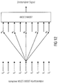
- the accompanying block diagram of a psychoacoustic audio decoder is in Fig. 24 to see.
- the Fourier transform is the most important method for analyzing the harmonic structure of a signal. It is part of the Fourier analysis and named after the French mathematician and physicist Jean-Baptiste-Joseph Fourier (1768-1830), who introduced it for the first time.
- the Fourier transform is a function for converting a time signal into its representation in the frequency domain. It is used, among other things, to describe and predict the behavior of linear time-invariant (LTI) systems (Burrus and Parks, 1985). For example, it plays a major role in acoustics and in the characterization of human hearing.
- x (t) is the signal to be analyzed in the time domain and X ( f ) is the corresponding Fourier spectrum in the frequency domain. It should be noted that the result is complex, although a real signal is transformed. Using Euler's relation in Equation 2.2, it can be shown that the real part of X ( f ) corresponds to the cosine pattern of x ( t ) and the imaginary part corresponds to the sine components.
- DFT discrete Fourier transform
- X [ k ] is the discrete, periodic spectrum of x [n] with ⁇ k . n ⁇ N .
- the period length of the spectrum corresponds to the transformation length N and normalized frequencies in the interval [0, 2 ⁇ ] are mapped.
- DFT For real input signals, DFT has an important property. It is not calculated as in the general case N independent frequency coefficients, but only half as many. This property can be exploited, for example, for the storage or transmission of the data.
- the computational effort of the DFT and IDFT is N 2 complex multiplications and additions. If symmetries are used in the calculation, the number of computation steps required is reduced to N ID N and the complexity corresponds to O ( N log N ). However, in the fast methods, the transformation length N must correspond to a power of two.
- the fast Fourier transformation is called FFT (Kiencke and Jäkel, 2005).
- the discrete Fourier transform has not prevailed in the field of data compression.
- the big disadvantages of the DFT are the high computational effort and the redundancy contained in the spectrum.
- efficient methods of calculating the DFT exist in the form of FFT, a complex spectrum is always generated.
- N complex values are calculated from N transformation values.
- only the first N / 2 spectral values contain new information.
- DCT Discrete Cosine Transform
- the DCT-II is primarily used as a transformation of image data. She is the first in the literature described type of DCT. Thus, the term “DCT” generally refers to DCT-II (Ahmed et al., 1974).
- the DCT-III is the inverse transformation to the DCT-II and vice versa.
- the DCT-IV is of particular importance. It is the basis of the modified discrete cosine transformation.
- the DFT calculates only N / 2 independent frequency coefficients from a real-valued signal of length N. Conversely, this means that 2 N values in the time domain are needed to obtain N spectral values. However, if only N time values are available, the signal must be continued in a suitable manner. Here, the symmetrical extension by reflection of the entire signal offers. The extended signal thus appears to be repeated with a period length of 2N. This has the advantage that the disturbing leakage effect of the DFT is suppressed with truncated signals (Kiencke and Jäkel, 2005).
- the DCT in contrast to the DFT, is a purely real transformation. This results in two advantages. Firstly, complex multiplications and additions do not need to be computed, and secondly, only half of the storage space is needed to store the data because there are no complex value pairs. Furthermore, it is noticeable that the DCT requires exactly N values for the transformation in order to calculate N independent frequency coefficients. The frequencies are all in the interval [0, ⁇ ]. In contrast to the DFT, the redundancy contained in the spectrum for real-valued input signals has disappeared and thus the frequency resolution is twice as high. The disadvantage, however, is that the DCT spectrum can not be converted into magnitude and phase.
- the signal contains frequencies that correspond to the DCT basis functions (see equations 2.14a to 2.14d), but are rotated by 90 ° in proportion to their phase. These frequencies are then not represented by the DCT, ie the DCT coefficient in question is zero. For these reasons, DCT is well suited for effective and fast data compression, but less for signal analysis (Malvar, 1992).
- DST discrete sine transformation
- the signal length of x [n] here corresponds to bN.
- block artifacts occur due to the quantization.
- a well-known example of such artifacts is the JPEG compression method.
- the origin of the block artifacts lies in the border continuations to be performed for the periodization. They do not correspond to the originally assumed signal continuations (see Equation 2.16).
- the result is discontinuities at the block boundaries that shift the energy to high frequencies in the frequency domain (Malvar, 1992). Jumps in an audio signal are perceptible as clicks. For such artifacts, human hearing is very sensitive. They must therefore be avoided.
- MDCT Modified discrete cosine transformation
- the redundancy can be removed by the overlap-add (OLA) method.
- OLA overlap-add
- the resulting blocks are superimposed to 50% and added up, this procedure is called Overlap Add.
- the frequency resolution of the MDCT can be further improved by weighting the input sequence x [ n + bN ] with a window function.
- the window corresponds to a rectangular function that cuts out the current block b from the total signal. In the frequency domain, this corresponds to a convolution with the si function.
- Equation 2.20 By substituting the window function w [2 N - 1 - n ] into Equation 2.20, another important property of the MDCT can be seen. The result corresponds to the discrete convolution of x [ n + bN ] with the modulated window function w [ n ].
- ⁇ k ⁇ [0, N - 1] Schottamp, 1996):
- the window function corresponds to the low-pass prototype FIR filter, which is modulated with the cosine kernel and thus represents the frequency bands of the filter bank. It follows that the input sequence x [ n + bN ] is decomposed into exactly N subbands. In connection with the TDA property, the MDCT meets the requirements of a so-called "critically sampled filter bank".
- Such a critically sampled filter bank is in Fig. 25 to see.
- Fig. 25 an N- band critically sampled PR filter bank with a system delay of n d samples.
- Such filter banks are particularly important for audio coding because they describe a signal with the least number of samples as accurately and completely as possible (Rao and Yip, 2001).
- ⁇ N corresponds to a reduction of the sampling rate by a factor of 1 / N and ⁇ N of a magnification by a factor of N.
- the signal after the synthesis filter bank x [ n ] x [ n -n d ] is identical to the input signal x [ n ] before the analysis filter bank are identical except for a constant delay of n d samples.
- h k [ n ] is the modulated window function w k [ n ] in the case of MDCT. Since w [ n ] satisfies the PR conditions, the analysis filters h k are identical to the synthesis filters g k .
- the operator T characterizes the transposition.
- the transformation rule can also be represented as a matrix.
- Every column of forms the MDCT spectrum of the respective block with index b in x .
- this form of MDCT needs 2N 2 multiplies and additions.
- the calculation effort can be significantly reduced.
- a FIR filter h [ n ] can always be in M ⁇ N Phases are divided if the length of the filter corresponds to an integer multiple of M.
- the m-th stage p m [n] h [n] is generated by h [n] delayed by z -m and the sampling rate is reduced by the factor M (Malvar, 1992).
- M Mem-var, 1992
- the MDCT is considered to be implemented according to the polyphase approach.
- BWE Bandwidth Extension
- Fig. 27 shows bandwidth extension categories (Larsen and Aarts, 2004).
- top left is shown low-frequency psychoacoustic BWE.
- High-frequency psychoacoustic BWE can be seen on the top right.
- bottom left is low-frequency BWE shown.
- lower right high-frequency BWE shown.
- the energy of band 'a' (dashed line) is pushed into band 'b' (dotted line).
- the spectral band replication is known from the prior art, as it is used inter alia in HE-AAC.
- SBR spectral band replication with SBR
- correlations between low and high frequency signal components are exploited to spectrally expand the low pass signal provided by the encoder.
- the low frequency bands of the underlying filter bank are copied to the missing high bands and the spectral envelope adjusted.
- This copying process causes perceptible artifacts, such as roughness and unwanted tone color change, especially at low cut-off frequencies. These are mainly caused by the lack of harmonic continuation of the spectrum at the boundary between baseband and the algorithmically generated high frequency bands.
- a prior art SBR audio coder uses pQMF subband decomposition of the signal, thus ensuring high coding efficiency [Ekstrand 2002]. This is achieved by transmitting only the lower frequency bands while reconstructing the higher frequency components using side information and the aforementioned frequency shift of the lower bands.
- Spectral band replication is currently the most widely used method for bandwidth expansion. It is used among others in HE-AAC and mp3PRO.
- SBR was developed by Coding Technologies to increase the efficiency of existing audio encoders. This is achieved by processing only frequencies below a certain corner frequency f g of an encoder. In the These examples use mp3 and AAC encoders as core encoders. Frequencies above the cutoff frequency are only described by a few parameters. Depending on the quality to be achieved, this is between 5kHz and 13kHz. In the receiver, the high frequency components are then reconstructed with the aid of this side information and the decoded band-limited signal (Ekstrand, 2002).
- Fig. 28 shows the block diagram of an extended SBR encoder.
- the sampling rate of the input signal is lowered and then fed to the actual encoder.
- the signal is analyzed by a complex quadrature mirror filter bank (QMF) and an energy calculation is performed.
- QMF quadrature mirror filter bank
- the used QMF consists of 64 subbands. From this, the required parameters for the estimation of the spectral envelopes can then be derived. Other parameters make it possible to respond to the specific characteristics of the input signal.
- the knowledge of the SBR encoder about high frequency band generation allows it to detect large differences between the original and synthesized high frequency (RF) components.
- the generated page information is inserted in the outgoing bit stream in addition to the actual audio data (Larsen and Aarts, 2004).
- Fig. 29 Figure 4 shows the block diagram of the associated SBR extended decoder.
- the band-limited audio data is decoded by the decoder and the control parameters are extracted from the bitstream. Subsequently, the audio data for the reconstruction of the high frequency components are returned to a QMF filter bank. Within this filter bank, the baseband is copied and inserted above the cutoff frequency (cf. Fig. 30 , Left).
- Fig. 30 schematically shows the magnitude frequency response. It is Fig. 30 a schematic representation of the SBR-RF reconstruction. In Fig. 30 , on the left a copying and moving of the baseband is shown. In Fig. 30 , right is a spectrum after the adjustment of the spectral envelope shown.
- the spectral envelope information generated in the SBR encoder is now used to match the envelope of the copied spectrum to the original one.
- This adaptation is based on the transmitted control parameters and the energy of the respective QMF band. Diverge the properties of the reconstructed spectrum of In addition to the original signal, additional tonal components or noise are added to the signal (Larsen and Aarts, 2004). In Fig. 30 On the right is the adapted reconstructed spectrum.
- the band-limited signal and the reconstructed high-frequency signal are combined and transferred through the synthesis filter bank in the time domain. In this way a bandwidth-extended signal has been created, which can now be reproduced.
- Fig. 31 shows a destruction of the harmonic structure in SBR.
- Fig. 31 on the left an original broadband spectrum is shown.
- Fig. 31 On the right is a spectrum after SBR RF reconstruction.
- harmonic signals such as a pitch pipe generates the SBR and equivalent bandwidth expansion techniques thereby avoiding unwanted artifacts such as tonal roughness and unsightly tones, as the harmonic structure of the signal is not completely preserved.
- using the SBR will introduce unwanted artifacts such as roughness and timbre changes.
- bandwidth extension techniques that avoid the problem of inharmonic spectral continuation.
- two of these methods are presented. In essence, these methods replace the RF generator of the SBR decoder Fig. 29 and thus represent an alternative to the simple copying process.
- the adjustment of the spectral envelope and the tonality remain unchanged. Since the input signal must be in the time domain, these methods are also referred to as bandwidth broadening time domain.
- the harmonic bandwidth extension can be called.
- Harmonic Bandwidth Extension uses a phase vocoder to produce the high frequency range.
- the spectrum is stretched.
- the baseband is spread to the maximum signal frequency f max and the frequency range between the cutoff frequency and f max . cut out.
- the spectrum then consists of this section and the baseband (cf. Fig. 32 , right).
- the envelope is adjusted as in SBR (Nagel and Disch, 2009).
- Fig. 32 is a schematic representation of HBE RF reconstruction.
- Fig. 32 on the left a stretching of the baseband by a factor of 2 is shown.
- Fig. 32 right is a spectrum after the adjustment of the spectral envelope shown.
- the disadvantage is that the spacing between the partials in the HF range changes with the extension factor as a result of the spread of the spectrum Fig. 33 can be seen.
- complex calculations are necessary to spread the spectrum. These include high-resolution DFT, phase adjustment and sample rate conversion (Dolson, 1986). If the audio signal is divided into blocks, an overlap add structure is additionally required in order to be able to continue the phase of the neighboring blocks continuously. For very tonal signals very good results can be achieved with the phase vocoder technique, but in the case of percussive signals the transients smear and it becomes necessary to perform a separate transient treatment (Wilde, 2009).
- Fig. 33 shows a harmonic structure in HBE.
- Fig. 33 on the left an original broadband spectrum is shown.
- Fig. 33 right spectrum is shown after the HBE RF reconstruction.
- CM-BWE Continuous Modulated Bandwidth Extension
- Fig. 34 shows a schematic representation of the CM-BWE-HF reconstruction.
- a modulation of the baseband with the frequency f mod is shown.
- Fig. 34 right is a spectrum after the adjustment of the spectral envelope shown.
- the modulation frequency must be adjusted for each modulation by choosing its nearest integer multiple (Nagel et al., 2010).
- the baseband must be filtered by a low-pass filter according to the modulation frequency so that the maximum possible signal frequency f max is not exceeded after the modulation. Similar to the methods already presented, the spectral envelope is subsequently formed and the tonality adjusted.
- CM-BWE In Fig. 35 the harmonic structure is to be seen, as it arises in a CM-BWE extended signal.
- Fig. 35 On the left is an original broadband spectrum.
- Fig. 35 right is a spectrum after the CM-BWE RF reconstruction shown.
- CM-BWE lacks a harmonic part-tone in the Spectrum. However, this is not disturbing because the harmonic structure is retained per se.
- the perceived quality of the reproduced audio signal should be comparable to the CD standard (sampling frequency 44100 Hz at 16-bit quantization depth). The quality should be maximized with decreasing data rate.
- the object of the present invention is achieved by a device according to claim 1, by a method according to claim 23 and by a computer program according to claim 24.
- a device for generating a frequency-shifted audio signal based on an audio input signal is provided.
- the audio input signal can be represented by one or more first subband values for a plurality of first subbands.
- the device comprises an interface and a frequency shifting unit.
- the interface is set up to receive the audio input signal.
- the frequency shifting unit is arranged to generate the frequency-shifted audio signal, wherein the frequency-shifted audio signal for a plurality of second subbands each has one or more second subband values. Further, each of the first and second subband values has information about each phase angle.
- the frequency shifting unit is further configured to generate one of the second subband values based on one of the first subband values such that the second phase angle of this second subband value is different from the first phase angle of this first subband value by a phase angle difference , wherein the phase angle difference depends on frequency information indicating which frequency difference the audio input signal is to be shifted to obtain the frequency shifted audio signal, and wherein the phase angle difference depends on a frequency bandwidth of one of the first subbands.
- Embodiments provide improved concepts for bandwidth extension, these improved concepts being referred to hereinafter as “harmonic spectral band extension” or “HSBE”.
- This developed harmonic bandwidth extension in the frequency domain makes it possible to suppress unwanted artifacts.
- the replicated spectrum is modulated so that the original harmonic structure is preserved.
- HSBE can be based on signal representation in the MDCT area, thus allowing an efficient implementation.
- the harmonically correct bandwidth expansion is achieved by copying the spectral values with subsequent modulation.
- the subband domain of MDCT is used, which is usually already implemented in audio encoders. In this way, the transformation does not add complexity or delay.
- the subband signals of lower frequencies are shifted to the corresponding higher frequency bands.
- every other sample of the subband signals to be copied is reversed in sign (increasing block index, in the direction of time). In this way, the Alias Cancellation Property of the MDCT Filterbank also works for the frequency shifted and copied signal.
- convolution-like processing is performed between adjacent subband signals, adding a weighted version of the one subband signal to the subband signal of a sub-band adjacent to it, so that it is the opposite Sign of the aliasing component has there, and so that the aliasing is compensated or reduced.
- the weights are chosen so that they correspond to the desired fractional frequency shift.
- an FIR filter structure for aliasing cancellation is provided in embodiments.
- the filter impulse responses required for this purpose are optimized by means of successive approximation and stored, for example, as a look-up table.
- the concepts provided build on and enhance existing bandwidth expansion methods. With this new method, it is possible to increase the quality of the reproduced audio material while maintaining the memory requirements. It is not affected the encoding process, but further developed the decoder. The developed method realizes a harmonic bandwidth extension. It builds on spectral band replication (SBR), as used in HE-AAC technology.
- SBR spectral band replication
- the provided inventive efficient spectral band replication concepts preserve the harmonic structure of the original spectrum and thus reduce the described artifacts of the known SBR technology.
- the harmonic spectral band enhancement presented here provides a powerful and efficient way to extend the band-limited spectrum of an audio signal while continuing the harmonic structure.
- the transformation of the MDCT coefficients into MDST spectral values constitutes another important element of the harmonic spectral band extension.
- Modern audio coders work exclusively in the MDCT area. Although the signal is described sufficiently accurately in its spectral representation, this information is not sufficient for the replication of the spectrum with HSBE.
- the required phase curve can only be modified by additional MDST coefficients.
- a transformation is introduced which allows a constant delay to be used to calculate the missing MDST coefficients as effectively as possible from the known MDCT values. In addition to an exact solution, a flawed but resource-saving alternative is presented.
- the modulation of the spectrum is important for the efficient replication of the spectrum.
- the spectrum is shifted by integer MDCT subbands and on the other hand for a fine resolution a modulation within the bandwidth of an MDCT subband performed.
- the resolution achieved with this technique is approximately 0.5 Hz. This allows the harmonic structure of the spectrum to be replicated very accurately.
- the lag frequency necessary for the determination of the modulation frequency may, for example, be provided by the encoder.
- a system, apparatus, or method or computer program is provided to generate a frequency shifted signal using subband decomposition, wherein for fractional subband bandwidth shifts, the subbands are multiplied by multiplication by a complex exponential function.
- the aliasing components are compensated or at least reduced by performing butterfly processing between adjacent subband signals.
- the frequency shift is performed in the subband domain of an audio coding system.
- the frequency shift is used to satisfy missing frequency components and / or spectral holes of a frequency representation of a signal in an audio coding system.
- the frequency shift in combination with the sample rate conversion is used to vary the playback speed while maintaining the pitch.
- the frequency is first increased by shifting the frequency and then the playback speed is reduced, the playback time of a certain amount of audio data is lengthened while the pitch remains the same. If, for example, the frequency is first reduced by shifting the frequency, and then the playing time of the particular amount of audio data is increased, then the playing time is shortened while the pitch remains the same.
- the concepts are used to finely tune a music signal.
- the concepts provided can be used to particular advantage in the context of Auto Tune. For example, should only small pitch changes of a digital music signal, for example frequency changes smaller than the bandwidth of a sub-band, such as smaller than an MDCT or a QMF sub-band, the concepts provided are particularly advantageous.
- the concepts are used to generate higher frequencies of a spectrum by copying or frequency shifting lower frequency portions of a spectrum.
- subband decomposition is Modified Discrete Cosine Transform (MDCT).
- MDCT Modified Discrete Cosine Transform
- the subband decomposition is a polyphase quadrature mirror filter bank (QMF).
- QMF quadrature mirror filter bank
- the concepts provided in the above embodiments may be realized, among others, as a system, a device or a method or a computer program.
- a method for generating a frequency-shifted audio signal based on an audio input signal, wherein the audio input signal for a plurality of first sub-bands can be represented by one or more first sub-band values.
- the method comprises:
- the frequency-shifted audio signal for a plurality of second subbands each having one or more second subband values, each of the first and second subband values having information about each phase angle, and wherein one of the second subband values is generated based on one of the first subband values such that the second phase angle of this second subband value may differ from the first phase angle of this first subband value by one phase angle difference, wherein the phase angle difference Difference depends on frequency information indicating by what frequency difference the audio input signal is to be shifted in order to obtain the frequency shifted audio signal, and wherein the phase angle difference depends on a frequency bandwidth of one of the first subbands.
- Fig. 1a shows a device 100 for generating a frequency-shifted audio signal based on an audio input signal.
- the audio input signal can be represented by one or more first subband values for a plurality of first subbands.
- the device comprises an interface 110 and a frequency shifting unit 120.
- the interface 110 is adapted to receive the audio input signal.
- the frequency shifting unit 120 is arranged to generate the frequency-shifted audio signal, wherein the frequency-shifted audio signal for a plurality of second subbands each has one or more second subband values. Further, each of the first and second subband values has information about each phase angle.
- the frequency shifting unit 120 is further configured to generate one of the second subband values based on one of the first subband values such that the second phase angle of this second subband value is a phase angle difference from the first phase angle of this first subband value the phase angle difference depends on a frequency information indicating which frequency difference the audio input signal is to be shifted, eg by what frequency difference the first subband values of the subbands of the audio input signal are to be shifted in order to obtain the frequency-shifted audio signal, and wherein the phase angle difference depends on a frequency bandwidth of one of the first subbands.
- the interface may be configured to receive the frequency information indicating which frequency difference the first subband values of the subbands of the audio input signal are to shift.
- Fig. 1b shows a device 150 according to an embodiment.
- the device 150 is adapted to generate a frequency-broadened audio signal.
- the device 150 is configured to generate the frequency-broadened audio signal by the device 150 generating the second subband values of the frequency-shifted audio signal, the frequency-broadened audio signal comprising the first subband values of the audio input signal and the second subband values of the frequency shifted audio signal.
- HSBE harmonic spectral band extension
- the harmonic spectral band extension uses a copy of the baseband to generate the RF component.
- the baseband is reproduced via a copying process in the high-frequency range.
- the baseband shift in HSBE is extended.
- the baseband is first copied also upwardly so that the frequency from 0 Hz to f then lies g.
- the resulting gap between the last harmonic of the frequency f ⁇ fg in the baseband and the frequency fg is then equalized by shifting the copied baseband down again, so that the harmonic structure is again continuous.
- a gap is avoided by omitting a harmonic part as in the time domain method.
- the bandwidth expansion process consists of two parts. One part is realized by a copying process in the MDCT area. The low-frequency MDCT coefficients are replicated by simple copying. The other part of the bandwidth extension, ie the preservation of the harmonic structure, is achieved by manipulating the phase. Therefore, phase information must be present for this step.
- the harmonic spectral band extension basically works with purely real MDCT coefficients. To change phase information, therefore, a transfer into a complex spectrum takes place. This is achieved by the MDCT MDST transformation provided here.
- the HF band is subjected to high-pass filtering.
- This filtering is very simple by presenting the signal as an MDCT coefficient, since the unwanted coefficients can be set to zero.
- this type of shift causes a band limitation of the synthesized signal.
- the original maximum signal frequency f max is not reached, but only the frequency f syn .
- the occurring gap between f max and f syn can be filled with noise if necessary.
- Fig. 2 the copying process including the harmonic adaptation is shown schematically. It shows Fig. 2 a schematic representation of the HSBE-HF reconstruction. In Fig. 2 , on the left a copy and move the baseband shown. In Fig. 2 , right is a spectrum after the adjustment of the spectral envelope shown.
- the necessary adaptation of the phase causes additional interference components in the signal. These are created by the advanced anti-aliasing filtering of complex MDCT / MDST spectral values suppressed. Finally, the spectral envelope is adapted to its original course by a suitable method.
- Fig. 3 is an HSBE decoder, so a HSBE extended decoder shown that results with the above procedure.
- Fig. 3 1 shows a device 300 for generating a frequency-shifted audio signal according to an embodiment.
- it may be an HSBE decoder, that is, a HSBE extended decoder.
- the device 300 has an interface 310 and a frequency shifting unit 320.
- the device 300 Between the interface 310 and the frequency shifting unit 320 is an MDCT / MDST transformation unit 315. Furthermore, the device 300 has a filter unit 330. Furthermore, the device 300 has a synthesis transformation unit 340, for example in the form of a filter bank and an envelope adaptation unit 350. Furthermore, the device 300 in the embodiment of the Fig. 3 a unit for calculating ⁇ and ⁇ (318).
- the MDCT / MDST transform unit 315 may be configured to obtain one or more first MDCT coefficients of the audio input signal, which are coefficients of Modified Discrete Cosine Transform of the audio input signal. These first MDCT coefficients may be obtained by the MDCT / MDST transformation unit 315 from the interface 310, for example.
- the MDCT / MDST transform unit 315 is configured to determine, based on one or more of the first MDCT coefficients of the audio input signal, one or more first MDST coefficients of the audio input signal which are coefficients of a Modified Discrete Sine Transform.
- the frequency shifting unit 320 may then be configured to generate second subband values based on each of the first subband values, wherein each of the first subband values is based on one of the first MDCT coefficients and one of the first MDST coefficients based on this first MDCT coefficient.
- the illustrated structure of the device 300 depends on the implemented algorithms. For use of this decoder in other environments, it may be necessary to perform the envelope reconstruction in the frequency domain.
- the corresponding block is then located directly in front of the MDCT / MDST synthesis filter bank.
- other components can be integrated, such as the tonality adjustment used in SBR.
- these methods have no effect on the general functional principle of the harmonic spectral band extension.
- Fig. 3 also results in the decoding process of a signal according to an embodiment that has been encoded in the MDCT domain.
- the decoded MDCT coefficients are first transformed into a combined MDCT / MDSE representation. This is helpful because the modulation of a complex spectrum will produce larger aliasing components only in every other subband. Therefore, compensation is required only in every other subband, this compensation being performed by means of the proposed aliasing compensation method.
- the RF generator shifts the complex frequency inputs from the MDCT / MDST transformation representation according to the desired shift, either decoded from the bitstream or at the decoder, or by external processes.
- the modulation term used is: e - jb ⁇ ⁇ 180 ° .
- b is the block index
- ⁇ is the frequency shift in degrees (a frequency shift of 180 ° corresponds to shifting to the middle of the next subband).
- the modulation term used is a complex exponential function.
- ⁇ is an angle in degrees which depends on the frequency difference by which the first subband values of the subbands are to be shifted.
- the single-sideband modulation to preserve the harmonic structure is realized in part by manipulating the phase.
- the phase response is of crucial importance.
- HSBE generally works in the real MDCT sector.
- the encoder provides only MDCT coefficients, so that the MDR coefficients are additionally required for the phase response.
- the conversion of the MDCT coefficients into the corresponding MDST coefficients is possible and will be explained below.
- the MDCT has a corresponding function for calculating the sine components in the signal: the Discrete Modified Sine Transform (MDST).
- MDST Discrete Modified Sine Transform
- a complex transfer function calculated from a combination of MDCT and MDST spectra is necessary, for example, to manipulate the phase response.
- the following presents the implemented method for converting the MDCT spectrum into MDST coefficients.
- X ⁇ MDST T ⁇ DST ⁇ D ⁇ ⁇ F ⁇ sin ⁇ F ⁇ T ⁇ D ⁇ - 1 ⁇ T ⁇ - 1 ⁇ X ⁇
- H ⁇ H ⁇ 0 z 0 + H ⁇ 1 z - 1 + H ⁇ 2 z - 2
- the three sub-matrices have characteristic features that lead to an efficient calculation.
- the matrix is a sparse matrix with the elements 0.5 and -0.5. Between the matrices and there is a direct connection, so that the matrix as a reflection of the elements of at their side diagonal produce. The exact shape and a detailed calculation of these matrices will be shown later.
- the matrices Upon closer examination of the matrices and It is noticeable that they contain very many values that tend towards zero.
- the coefficients with the largest values in value concentrate on a narrow area near the main diagonal of the matrices. It therefore makes sense to set the remaining coefficients to zero in order to save both computing power and memory requirements.
- the values on the diagonals are very similar. They differ essentially only by their sign from each other. Only in the areas near the corners do the coefficients take on larger values.
- a simplified matrix is now determined whose values are from the middle column of the matrix be removed. For this purpose, an area is cut from the middle column, which includes the element of the main diagonal and any number of other elements below the main diagonal. This section is called h [ n ].
- the middle column of the new matrix will be formed around the of h [n] and a point reflection of h [n] on the main axis member h i j, the rest of the column is zero.
- the other columns of the simplified matrix are now formed by a cyclic shift of this column. The sign of every other column is adjusted.
- the required storage space for the transformation matrix has dropped to 20% by mirroring the values of h [ n ].
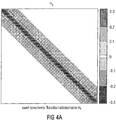
- Fig. 4A and 4B represent an estimate of the MDCT MDST transformation matrix.
- Fig. 4A is the fully occupied matrix to see and compare in Fig. 4B the simplified matrix H ⁇ 0 ' in symmetrical Toeplitz-like structure.
- the simplification makes a large part of the coefficients away from the main diagonal of H ⁇ 0 ' equals zero.
- An advantage of the HSBE process is the maintenance of the harmonic structure after bandwidth expansion. As already mentioned, this is done by a phase manipulation in the complex MDCT / MDST range.
- B f max - f g .
- the aim is to shift the spectrum downwards so that the first harmonic in this band (for example, at the frequency f H, n > f g ) after the shift at the highest harmonic frequency in the baseband has the frequency f H, ⁇ ⁇ f g comes to rest.
- the spacing of the frequencies f H, n and f H, ⁇ is referred to as lag frequency f lag . This frequency regulates the adaptation of the harmonic structure.
- This frequency can also be represented as a corresponding integer and non-integer multiple of MDCT subbands by which the frequency band is to be shifted down. This provides maximum flexibility of the developed process allows. After the above condition is reached, all MDCT coefficients with a discrete frequency less than f g are set to zero so that baseband and shifted band do not overlap.
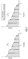
- Fig. 7 shows the desired result of the HSBE method for a tonal signal.
- Fig. 7 shows the harmonic structure at HSBE.
- Fig. 7 on the left the original broadband spectrum is shown.
- Fig. 7 On the right the spectrum is shown after the HSBE HF reconstruction.
- the preservation of the harmonic structure is complicated when an MDCT band has a high bandwidth compared to the frequency difference of successive partials of the harmonic structure. If the modulation is performed only at frequencies which are an integer multiple of the bandwidth of an MDCT band, the resolution of the harmonic reconstruction is then severely limited, and hence a fine harmonic structure can not be restored. It is therefore necessary to allow high accuracy of the modulation so that the spectrum of the baseband can be modulated not only by integer multiples of the MDCT band bandwidth but also by fractions thereof.
- the following approach makes it possible to shift the spectrum within the bandwidth of an MDCT subband.
- the method is based on a modification of the phase of the complex MDCT / MDST spectrum.
- the phase is rotated as a function of the time profile of the signal by a normalized frequency shift ⁇ .
- This temporal rotation of the phase angle thus allows a very fine shift of the spectrum.
- X mod b X b ⁇ e - j ⁇ b ⁇ ⁇ ⁇ ⁇ 180 °
- X (b) is the b-th column of the complex matrix
- X ⁇ X ⁇ MDCT + j ⁇ X ⁇ MDST and ⁇ the normalized frequency shift in degrees.
- ⁇ arbitrary angles are possible for ⁇ , but for practical reasons, the range of values is very limited and is in the interval - 90 . 90 ⁇ Z , It is possible with this interval to compute modulations covering the bandwidth of an MDCT band. By setting the normalized frequency shift to the specified interval, the spectrum can be shifted by half the MDCT band bandwidth to either high or low frequencies.
- ⁇ is an angle in degrees which depends on the frequency difference by which the first subband values of the subbands are to be shifted.
- a second subband value to be determined can then be determined by multiplying one of the first subband values in X ( b ) by the result value.
- the limited value range of the phase angle ⁇ allows with the introduced modulation only the shift of the spectrum of at most the bandwidth of an MDCT band. For shifts in the spectrum of the bandwidth of an MDCT band, this shift is split into two parts, an integer multiple of the MDCT band bandwidth and a fraction of that bandwidth. First, the spectrum is modulated by the necessary frequency smaller than the bandwidth of an MDCT band according to Equation 4.12 and then the spectrum is shifted by whole spectral values.
- This vector element cut corresponds to the high-pass filtering of the complex MDCT / MDST spectrum discussed above.
- the modulation frequency as a function of f lag is converted into the modulation index ⁇ and the phase angle ⁇ .
- the frequency f lag is normalized to half the sampling frequency f s .
- the patch ratio is the ratio of the maximum possible signal frequency f max to the cutoff frequency of the baseband fg.
- a patch ratio of 2: 1 for example states that a single copy of the baseband is created and modulated (cf. Fig. 2 ). Patch ratios greater than 2: 1 occur at low or fluctuating transmission rates. Such ratios are realized similar to the CM-BWE (see above) by copying and modulating the baseband several times.
- CM-BWE see above
- Fig. 8 represents a scheme of extended HSBE-RF reconstruction. In Fig. 8 on the left is copying and moving the baseband. In Fig. 8 , right is the spectrum after the adjustment of the spectral envelope to see.
- the following describes concepts for suppressing occurring interference components.
- the concepts described here can be used, for example, in the filter unit 330 of FIG Fig. 3 come into use.
- the frequency of the original sinusoid ( y ref ) corresponds to the band center of the 12th MDCT band.
- the entire spectrum is modulated by the selected phase angle by a quarter of the bandwidth of an MDCT band towards high frequencies.
- the eight dominant aliasing components lie in every second band below and above the 12th MDCT band. This property of aliasing components is given for any signal. This is because each signal can be decomposed into a weighted sum of sine and cosine oscillations (see above).
- Equation 4.12 For each of these partial oscillations, the modulation according to Equation 4.12 produces this special pattern of the aliasing components. With this knowledge, a method can be developed that allows to free any signal from the unwanted spurious components. It is sufficient to analyze and cancel the aliasing components resulting from the modulation of a sinusoidal signal.
- the following provides concepts for anti-aliasing filtering.
- the temporal overlap of the blocks for the TDA generates additional signal components in the frequency domain. These are present as interference components in the spectrum of the bandwidth-expanded signal, since they are not extinguished during the inverse transformation due to the shift in the frequency domain.
- These interferers which are recognizable as peaks in the FFT spectrum (cf. Fig. 9 ) are represented in MDCT by the small stopband attenuation of the DCT-IV filter bank of only about 15 dB by a sum of contributions in several of the overlapping MDCT bands.
- the energy of the interferers in the high-resolution DFT spectrum can therefore be regarded as a summation of the energy of several MDCT bands.
- a filter is provided to reduce the noise components in the MDCT area.
- the filter is based on a sequential summation of the frequency values weighted by the filter coefficients.
- the expansion of the filter by a centered frequency value represents the frequency range in which the interference components are extinguished.
- Each dominant aliasing component requires a filter coefficient that minimizes it.
- H ( ⁇ ) is the real anti-aliasing filter for a given phase angle ⁇ and X (b) is the complex MDCT / MDST spectrum.
- the spectrum after filtering ( X A ntiAlias (b) ) is longer than the original spectrum X (b). Therefore, the spectrum should be trimmed so that it again corresponds to the transformation length N. It removes the part of the spectrum where the filter goes in and out. This will be on At the beginning and at the end, the folding product in the complex MDCT / MDST area is cut by half the filter length.
- AAF anti-aliasing filter
- the filter coefficients of Fig. 10 thus have an orderly order. Each filter coefficient in this order, following a non-zero filter coefficient, has the value zero.
- the successive approximation is an iteration method of numerical mathematics and describes the process of the gradual approximation of a computational problem to the exact solution.
- a calculation method is used repeatedly and the result one step as the initial value for the next step.
- the result of the results should converge. If the acceptable error for the exact solution is minimal, the result is determined with sufficient accuracy (Jordan-Engeln and Reutter, 1978).
- an analysis signal with equation 4.12 is modulated by a specific phase angle ⁇ .
- the analysis signal is a sine wave for the reasons mentioned above.
- the frequency of the sound is ideally one quarter of the underlying sampling frequency. This has the advantage that the resulting aliasing components up to the fourth order have the greatest possible distance to the edges of the spectrum and do not interfere with other noise components.
- an MDCT transformation length of 32 samples is ideal.
- the frequency of the sine wave corresponds to the band center of the sixteenth MDCT band.
- the restriction to this transformation length offers some advantages. This reduces the calculation effort of the MDCT.
- the aliasing components are generated up to the fourth order without interference with maximum distance from each other. This is particularly advantageous for the necessary signal peak detection.
- the signal peak detection automatically detects the aliasing components to be suppressed in the high-resolution DFT magnitude frequency response.
- the aliasing components are successively optimized in an alternating sequence. This is necessary because the interfering components influence each other. It proceeds from the weakest fourth-order component to the most dominant first order. This ensures that the first-order aliasing components receive the greatest possible attenuation.
- the direct component ie the spectral value for which the aliasing components are to be canceled, a one is set in the filter. This value is not changed during optimization.
- the actual numerical optimization takes place according to the illustrated principle of successive approximation.
- An initial value is assigned to the filter coefficient to be optimized, all other coefficients except the direct component remain zero.
- the complex MDCT / MDST spectrum is folded with this filter and the magnitude frequency response is examined for a reduction of the relevant interference component. If this is the case, the filter coefficient is increased according to the set increment. This investigation and increase procedure is repeated until no more suppression of this aliasing component is possible. Subsequently, the following filter coefficients are used in the same way, where already optimized filter coefficients are maintained.
- X AntiAlias is a filtered signal with suppressed interfering components.
- X Alias is the spectrum of the modulated signal and X AntiAlias that of the modulated signal, folded with the optimized filter for the corresponding phase angle.
- the peaks in the spectrum marked with peak recognition are the aliasing components detected by the signal peak detection , including the direct component (fourth detected peak from the left).
- the numerical optimization of the filters reduces the noise components in this example on average to -103 dB.
- the required filter can then be loaded from a database.
- the filter coefficients of the filter can be read out of a database or a memory of a device for generating a frequency-shifted audio signal as a function of the phase angle.
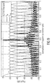
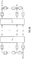
- Fig. 12 shows the butterfly structure. The weights are determined by successive approximations.
- Fig. 12 shows the aliasing reduction for the subband X 4 (black line). The same procedure should be followed for all modified subbands. To reduce caused by the modulation of X 4 of the aliasing component, X 4 is where to be multiplied with the weights to w 4 to the sub-band signals X 0, X 2, X 4, X 6 and X 8 add. It should be noted that the weight w 2 is always 1.
- this means: In order to produce a filtered subband value of one of the subbands, a sum of the unfiltered subband value of this subband and further summands is to be formed. (the weight / filter coefficient w 2 applied to the unfiltered subband value of this subband is w 2 1).
- the further summands are weighted subband values, namely in each case a subband value of other subbands, which have been multiplied or weighted by the other weights / filter coefficients.
- the reconstruction of the spectral envelopes takes place via LPC filtering.
- the tonal components of the signal are removed in the encoder by a linear prediction filter and transmitted separately as LPC coefficients.
- the required filter coefficients can be calculated by Levinson-Durbin recursion (Larsen and Aarts, 2004).
- the baseband in the decoder acquires a white spectral characteristic.
- an inverse filtering with the LPC coefficients is carried out, so that the original spectral envelope is impressed on the signal again.
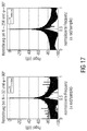
- Fig. 13 shows an HSBE-LPC envelope adjustment.
- X represents a BWE signal before the envelope adjustment .
- X iLPC is a BWE signal after the envelope adjustment .
- Fig. 13 to see the DFT magnitude frequency responses of an HSBE bandwidth-expanded signal.
- the signal X Before the reconstruction of the spectral envelope, the signal X has the mentioned white signal characteristic.
- the envelope After the adaptation of the envelope by the inverse LPC filtering, the envelope corresponds to the original spectral characteristic.
- Bandwidth expansion using continuous single-sideband modulation is a time domain method. Therefore, a time signal is always required for the application. Since envelope and tonality matching takes place after the bandwidth expansion, for which in each case a signal in the spectral range is required, the bandwidth-expanded signal must be transformed back into the frequency range when using the CM-BWE method. This transformation into the time domain and again into the frequency domain is omitted in the harmonic spectral band extension, since it works in the MDCT / MDST range.
- the time signal must be converted to an analytic signal prior to application of continuous single-sideband modulation.
- the calculation of the required analytical signal is problematic since it is realized via a Hilbert transformer.
- the ideal transfer function of the Hilbert transform is the sign function. This function can only be displayed in the time domain with an infinitely long filter. With a realizable finite impulse response filter, only approximation of the ideal Hilbert transformer is possible.
- the signal is not perfectly analytic after the approximate Hilbert transform. The quality of the calculated pseudo-analytic signal therefore depends on the length of the filter used.
- the efficiency of the new harmonic spectral band extension depends on the required computational effort and storage space. The investigation of these factors is based on the implementation of the algorithm in the programming language C. In the algorithmic implementation, much emphasis is placed on minimizing the number of calculation steps. Nevertheless, the most computationally intensive steps include the transformation of the MDCT coefficients into MDST spectral values as well as the anti-aliasing filtering.
- the modulation for harmonically correct replication of the spectrum is comparatively simple since the shift by the modulation index ⁇ corresponds to only one copying process and the phase rotation by the angle ⁇ can be reduced to a complex multiplication per spectral value.
- the adaptation of the spectral envelope is not included in this consideration. Since no evaluation is an integral part of the HSBE process, it is not implemented algorithmically.
- Table 5.1 summarizes the spectrum modulation and filtering results. They refer to the function local_HSBEpatching (), in which the corresponding algorithms are implemented. Table 5.1 N 2 4 8th 16 32 64 128 256 512 1024 2048 ADD 4 8th 16 32 64 128 256 512 1024 2048 4096 SECTION 1 1 1 1 1 1 1 1 1 1 1 MULT 6 12 24 48 96 192 384 768 1536 3042 6144 MAC 16 32 64 128 256 512 1024 2048 4096 8192 16384
- Table 5.1 tabulates the complexity of HSBE modulation and anti-aliasing filtering.
- the listing includes the number of relevant operations as a function of transformation length N.
- N 2048, of which 2 N additions and 3 N multiplications. Much higher is the cost of the required aliasing cancellation out.
- 16384 MAC operations are performed. This corresponds to the number of non-zero elements of the anti-aliasing filter multiplied by the transformation length, in this case 8 N (compare the comments on anti-aliasing filtering above). This result results in a linear relationship with the complexity O ( N ) for the computation effort of the modulation and the AAF.
- Fig. 14 this relationship is shown graphically. It puts Fig. 14 the complexity of HSBE modulation and anti-aliasing filtering.
- Fig. 15 shows the complexity of fast MDCT / MDST. It should be noted that two inverse transformations must be calculated for the transition of the signal from the complex MDCT / MDST range to the time domain. The number of required operations is doubled.
- Table 5.5 - Memory usage by HSBE module elements Size in bytes Size in KiB hsbelib 20480 81920 80 Hmatrix 4194304 (205) 16777216 (820) 16384 (0.80) hsbeCanv 15 60 0.05 fastDCSTIV 3072 12288 12 fastDCSTIII 4096 16384 16 AAFdatabase 2715 10860 10.61 total 4224682 (30583) 16898728 (122332) 16502,66 (119,46)
- the harmonic spectral band extension implementation is based on single-precision floating-point arithmetic (single precision), so a floating-point number is represented as 32 bits.
- the number given in Table 5.5 thus refers to the number of floating-point numbers needed in this module.
- the memory utilization for the actual HSBE algorithm with about 109 KiB for the modulation, aliasing-canelation and MDCT / MDST is comparatively low.
- the database for the anti-aliasing filters is stored as a look-up table and requires just under 11 KiB for the total of 2715 filter coefficients.
- the decisive influence on the memory requirement is formed by the transformation matrix This matrix uses about 16 MiB of memory.
- the transformation length N represents a positive integer power of the number two.
- the maximum possible block length is limited to 2 11 , ie 2048, based on AAC.
- HSBE it is also possible to vary the block length during runtime. This is especially necessary for transient treatment in modern audio coders.
- the SNR is largely determined by the block length. It is true that large transformation lengths lead to a better result than very short block lengths. This is due to the modulation aliasing components. Although the anti-aliasing filtering suppresses interferers up to the fourth order, some unwanted components remain in the signal.
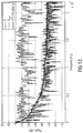
- Fig. 17 shows a residual disturbance in HSBE as a function of the transformation length.
- the harmonic spectral band extension provides a very accurate reconstruction of the harmonic structure of the signal.
- the resolution of the developed method is in the range of approximately 0.5 Hz. This means that the spectrum can be accurately modulated to a half hertz. For smaller sampling frequencies or larger block lengths, the resolution increases and the modulation is feasible in even finer areas.
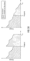
- the result of applying HSBE to a multi-sine wave signal is in Fig. 18 shown.
- Fig. 18 shows a comparison of the HSBE with the SBR.
- REF FreqGang denotes a spectrum of the original multi-sine signal.
- SBR FreqGang denotes an SBR bandwidth-expanded signal;
- HSBE FreqGang refers to a bandwidth-enhanced signal using HSBE.
- the spectrum is exactly reconstructed with the developed HSBE method.
- HSBE FreqGang band-limited signal with HSBE
- the spectrum is exactly above the original spectrum (REF FreqGang).
- the corresponding spectrum is shown, which is not harmonically adjusted (SBR FreqGang).
- SBR FreqGang harmonically adjusted
- the DCT-II is derived from the DFT in Equation 2.10 with Equation 2.12 (see also Rao and Yip, 2001).
- This relationship can also be used to calculate the DCT effectively using FFT (see Ahmed et al., 1974).
- the folding matrices needed to calculate the MDCT (see Equation 2.35) , and consisted of a delay matrix and the window matrix together.
- the window matrix contains the coefficients of the window function w [ n ] arranged in diamond structure.
- the inverse delay matrix is multiplied by the delay z -1 .
- the delay of the MDCT filter bank is justified therein (Schuller and Smith, 1996).
- the transformation matrix is required to convert the MDCT spectrum into the associated MDST spectrum.
- H ⁇ T ⁇ DST ⁇ D ⁇ ⁇ F ⁇ sin ⁇ F ⁇ T ⁇ D ⁇ - 1 ⁇ T ⁇ - 1
- H ⁇ z H ⁇ ⁇ F ⁇ ' ⁇ T ⁇ ' - 1 z
- a .11 a T ⁇ ' z 0 + T ⁇ ' z - 1 ⁇ F ⁇ ' ⁇ T ⁇ ' - 1 z 0 + T ⁇ ' - 1 z - 1
- a .11 b T ⁇ ' z 0 ⁇ F ⁇ ' + T ⁇ ' z - 1 - F ⁇ ' ⁇ T ⁇ ' - 1 z 0 + T ⁇ ' - 1 z - 1
- a .11 c T ⁇ ' z 0 ⁇ F ⁇ ' + T ⁇ ' - 1 z 0 + T ⁇ ' z - 1 - F ⁇ ' ⁇ T ⁇ ' - 1 z 0 + ⁇ + T ⁇ ' z 0 ⁇ + T ⁇ ' z -
- H ⁇ z 0 T ⁇ z 0 ⁇ F ⁇ ' ⁇ T ⁇ ' - 1 z 0
- H ⁇ 2 ⁇ ⁇ N ⁇ H ⁇ 0 T ⁇ ⁇ ⁇ N
- ⁇ ⁇ N 0 ... 0 1 0 ... 1 0 ⁇ , , ⁇ ⁇ 1 ... 0 0
- Equation A.16 can be considered as a reflection of the values of matrix on its side diagonal be interpreted. With these properties can now be the effort to calculate from operations that were originally 4 N 3 (see Equation A.11d) to a quarter of them.
- the implementation of the DCT-IV is based on the fast DCT-IV algorithm.
- the advantage of this implementation is the efficient calculation of the transformation and the associated short algorithmic delay.
- At the heart of DCT-IV are two parallel DCT-III transformations according to Equation 2.14c. This is similar to the FFT of a so-called butterfly and a pipeline structure together (Rao and Yip, 2001).
- the complexity of this algorithm is O ( N log N ) and is comparable to the required computational effort of the FFT.
- the exact structure of the DCT-III is in Fig. 19 shown. Specially shows Fig. 19 a fast universal DCT-III / DST-III structure (Rao and Yip, 2001)
- the input sequence x n thus becomes the DCT-II spectral values transferred. Since DCT-III is the inverse transformation to DCT-II, both transformations can be calculated using this structure.
- This universal structure for the calculation of the DCT-III / DST-III and the associated inverse transformations DCT-II and DST-II forms the basis for the DCT-IV according to Equation 2.14d.
- Fig. 20 the structure of the implemented DCT-IV can be seen. It shows Fig. 20 a fast DCT-IV structure (Rao and Yip, 2001)
- the structures shown can be implemented, for example, in the programming language C.
- the corresponding functions are dct_processor () for the universal DCT-III / DST-III (DCT-II / DST-II) as well as fdcstivld () for the fast DCT-IV / DST-IV.
- Matlab does not implement a fast version of these transformations because the performance of the algorithm is irrelevant.
- decoder_hsbe is a harmonic spectral band extension (HSBE) decoder.
- HSBE harmonic spectral band extension
- [y varargout] decoder_hsbe (X_core, T_idct, G, sideinfo, ... aaf_dat, b_noisefill, b_useMDST);
- the filters are available as FIR filters in a database.
- the database is saved as a .mat file and contains a one-dimensional struct. Each entry in the database consists of the angle specification for which the FIR filter is to be used and the filter coefficient as a vector.
- AAFoptimizer generates an anti-aliasing filter (AAF) as an FIR filter.
- AAF anti-aliasing filter
- fir x_antialias AAFoptimizer x .
- HSBEprocessing is the main interface of the created static library hsbe.lib for the bandwidth extension via HSBE.
- a signal excerpt in the time domain is transformed by MDCT / MDST and spectrally so extended to maintain the harmonious structure.
- the complex bandwidth-extended signal is again transferred to the time domain and output.
- Envelope reconstruction as in the Matlab function decoder_hsbe () does not take place.
- HSBE_RESULT HSBEprocessing (HSBE_HANDLE HSBEhandle, ... float * pSamplesIn, float * pSamplesOut, ... unsigned short nSamplesIn, float frequencyOffset);
- HSBEinit is the function to initialize HSBE.
- the required memory is reserved, the window function calculated and the MDCT-MDST transformation matrix calculated.
- all required parameters for HSBEprocessing () are entered in the handle.
- HSBE_RESULT HSBEinit (HSBE_HANDLE * HSBEhandle, ... unsigned short nSamplesIn, float f_core, float f_hsbe, ... unsigned char windowtype, char flags);
- HSBEfree releases the resources requested by HSBEinit ().
- embodiments of the invention may be implemented in hardware or in software.
- the implementation may be performed using a digital storage medium, such as a floppy disk, a DVD, a Blu-ray Disc, a CD, a ROM, a PROM, an EPROM, an EEPROM or FLASH memory, a hard disk, or other magnetic disk or optical memory are stored on the electronically readable control signals that can cooperate with a programmable computer system or cooperate such that the respective method is performed. Therefore, the digital storage medium can be computer readable.
- some embodiments according to the invention include a data carrier having electronically readable control signals capable of interacting with a programmable computer system such that one of the methods described herein is performed.
- embodiments of the present invention may be implemented as a computer program product having a program code, wherein the program code is operable to perform one of the methods when the computer program product runs on a computer.
- the program code can also be stored, for example, on a machine-readable carrier.
- an embodiment of the method according to the invention is thus a computer program which has a program code for performing one of the methods described herein when the computer program runs on a computer.
- a further embodiment of the inventive method is thus a data carrier (or a digital storage medium or a computer-readable medium) on which the computer program is recorded for carrying out one of the methods described herein.
- a further embodiment of the method according to the invention is thus a data stream or a sequence of signals, which represent the computer program for performing one of the methods described herein.
- the data stream or the sequence of signals may be configured, for example, to be transferred via a data communication connection, for example via the Internet.
- Another embodiment includes a processing device, such as a computer or a programmable logic device, that is configured or adapted to perform one of the methods described herein.
- a processing device such as a computer or a programmable logic device, that is configured or adapted to perform one of the methods described herein.
- Another embodiment includes a computer on which the computer program is installed to perform one of the methods described herein.
- Another embodiment according to the invention comprises a device or system adapted to transmit a computer program for performing at least one of the methods described herein to a receiver.
- the transmission can be done for example electronically or optically.
- the receiver may be, for example, a computer, a mobile device, a storage device or a similar device.
- the device or system may include a file server for transmitting the computer program to the recipient.
- a programmable logic device eg, a field programmable gate array, an FPGA
- a field programmable gate array may cooperate with a microprocessor to perform one of the methods described herein.
- the methods are performed by any hardware device. This may be a universal hardware such as a computer processor (CPU) or hardware specific to the process, such as an ASIC.
Description
Die vorliegende Erfindung bezieht sich auf Audiosignalverarbeitung und, im Speziellen, auf eine Vorrichtung, ein Verfahren und ein Computerprogramm für beliebige Frequenzverschiebungen in der Subband-Domäne.The present invention relates to audio signal processing and, more particularly, to an apparatus, method and computer program for arbitrary frequency shifts in the subband domain.
In der von neuen Medien geprägten Gesellschaft sind rechnergestützte Datenverarbeitungssysteme ein fester Bestandteil des täglichen Lebens. Schon seit einiger Zeit finden sich fast in jedem Haushalt Systeme zum Konsum neuer Medien wieder. Beispiele für solche Systeme, die Daten in digitaler Form übermitteln und wiedergeben, sind Abspielgeräte für Video- und Audiodaten, wie etwa für die DVD und BluRay, für die CD und das Dateiformat mp3. Diese Wiedergabesysteme zeichnen sich durch nahezu verlustfreie Reproduktion der medialen Inhalte aus. Neben der klassischen Telekommunikation stellt das Internet ein wichtiges Portal für die Kommunikation, beispielsweise mittels VoIP, dar. Die genannten Technologien werden alle durch die zugrundeliegende digitale Signalverarbeitung verbunden. Sie ist für die Qualität der Wiedergabe und Effizienz der digitalen Technologien von entscheidender Bedeutung.In a society dominated by new media, computer-aided data processing systems are an integral part of everyday life. Already for some time, almost every household has systems for the consumption of new media. Examples of such systems which transmit and reproduce data in digital form are video and audio data players such as the DVD and BluRay, the CD and the mp3 file format. These playback systems are characterized by almost lossless reproduction of the media content. In addition to classical telecommunications, the Internet is an important portal for communication, for example by means of VoIP. The above-mentioned technologies are all connected by the underlying digital signal processing. It is crucial for the quality of the reproduction and efficiency of digital technologies.
Audiosignalverarbeitung wird dabei immer wichtiger. Derzeit gibt es auf dem Markt eine Vielzahl an Audiocodern, z.B. realisiert durch Algorithmen zur digitalen Aufbereitung von Audiomaterial zur Speicherung oder Übertragung. Ziel jedes Codier-Verfahrens ist es, den Informationsgehalt eines Signals so zu komprimieren, dass es ein Minimum an Speicherplatz benötigt und gleichzeitig eine größtmögliche Reproduktionsqualität erhalten bleibt. Die Effizienz moderner Audiocoder richtet sich in erster Linie nach dem benötigten Speicherplatz und unter anderem nach dem benötigten Rechenaufwand des Algorithmus.Audio signal processing is becoming increasingly important. Currently, there are a variety of audio coders on the market, e.g. realized by algorithms for digital processing of audio material for storage or transmission. The goal of any encoding process is to compress the information content of a signal in such a way that it requires a minimum of storage space while maintaining the highest possible reproduction quality. The efficiency of modern audio coders depends primarily on the required storage space and, among other things, on the required calculation effort of the algorithm.
Ein digitaler Audiocoder ist prinzipiell ein Instrument zur Überführung von Audiosignalen in ein zur Speicherung oder Übertragung geeignetes Format. Dies geschieht auf Senderseite des Audiocoders (Encoder). Die so erzeugten Daten werden dann im Empfänger (Decoder) wieder in ihre ursprüngliche Form zurückgeführt und entsprechen im Idealfall den Originaldaten bis auf eine konstante Verzögerung (engl. Delay). Das generelle Ziel von Audiocodern ist die Minimierung der zur Repräsentation des Audiosignals benötigten Datenmenge bei gleichzeitiger Maximierung der empfundenen Wiedergabequalität. Bei der Entwicklung von Audiocodern muss also auf eine Reihe von Faktoren wie Wiedergabetreue, Datenrate und Komplexität geachtet werden. Daneben spielt auch das durch die Bearbeitung des Signals hinzugefügte Delay (die hinzugefügte Verzögerung) eine wichtige Rolle (Bosi und Goldberg, 2003).A digital audio coder is in principle an instrument for transferring audio signals into a format suitable for storage or transmission. This happens on the transmitter side of the audio encoder (encoder). The data thus generated are then returned to their original form in the receiver (decoder) and ideally correspond to the original data except for a constant delay (English: Delay). The general goal of audio coders is to minimize the amount of data needed to represent the audio signal while maximizing perceived ones Playback quality. Developing an audio coder requires a number of factors such as fidelity, data rate, and complexity. In addition, the delay added by processing the signal (the added delay) also plays an important role (Bosi and Goldberg, 2003).
Gerade in den Anfängen der Audiocodierung war die Effizienz der Verfahren von großer Bedeutung, da nur sehr begrenzt Speicher und Rechenleistung zur Verfügung standen. Heutzutage scheint dieser Anspruch nicht mehr gegeben. Selbst Heim-PCs oder Laptops können aufwändige Algorithmen mühelos in Echtzeit berechnen und Breitband-Internetverbindungen stellen ausreichend Bandbreite für die Übertragung von codiertem Audiomaterial zur Verfügung. Dennoch ist die Weiterentwicklung von Audiocodierverfahren von besonderer Bedeutung. Im Bereich der mobilen Kommunikation und der Satellitenübertragung ist die Bandbreite stark begrenzt. Es ist wichtig, die zu übertragende Datenmenge zu reduzieren. Es wird zudem in diesen Bereichen viel Wert auf die Effizienz der verwendeten Codier-Technologie gelegt. Die zugrundeliegenden Algorithmen müssen einfach strukturiert sein, um Rechenleistung und Stromverbrauch zu minimieren.Especially in the early days of audio coding, the efficiency of the processes was of great importance, since only very limited memory and computing power were available. Nowadays, this claim does not seem to exist anymore. Even home PCs or laptops can effortlessly compute complex algorithms in real-time, and broadband Internet connections provide sufficient bandwidth for the transmission of encoded audio material. Nevertheless, the further development of audio coding is of particular importance. In the area of mobile communication and satellite transmission, the bandwidth is very limited. It is important to reduce the amount of data to be transferred. In addition, in these areas, much emphasis is placed on the efficiency of the coding technology used. The underlying algorithms need to be simply structured to minimize computational power and power consumption.
Ein anderer Aspekt ist die Qualität der reproduzierten codierten Audiosignale. Viele Audiocoder reduzieren die Datenmenge über Irrelevanzreduktion. Dabei gehen in Abhängigkeit der Datenrate Signalanteile verloren. Bei niedrigen Datenraten sinkt damit die Qualität wiedergegebener Audiosignale.Another aspect is the quality of the reproduced coded audio signals. Many audio coders reduce the amount of data via Irrelevanzreduktion. In this case, signal components are lost depending on the data rate. At low data rates, this reduces the quality of reproduced audio signals.
Generell kann zwischen zwei Arten der Audiocodierung unterschieden werden, der verlustfreien und der verlustbehafteten Audiocodierung. Die verlustfreie Audiocodierung ermöglicht auf Empfängerseite eine exakte Rekonstruktion des ursprünglichen Signals. Dagegen verursacht das verlustbehaftete Verfahren über ein Modell der subjektiven Wahrnehmung irreversible Abweichungen gegenüber dem Originalsignal (Zölzer, 2005).In general, two types of audio coding can be distinguished, lossless and lossy audio coding. The lossless audio coding on the receiver side allows an exact reconstruction of the original signal. In contrast, the lossy process via a model of subjective perception causes irreversible deviations from the original signal (Zölzer, 2005).
Die verlustfreie Audiocodierung basiert auf der Verminderung der Redundanz, die im zu codierenden Signal enthaltenen ist. Ein gängiges Verfahren dazu ist zum Beispiel die lineare Prädiktion (engl. Linear Predictive Coding, LPC) in Verbindung mit nachfolgender Entropiecodierung. Solche Audiocodierverfahren ermöglichen die bitgenaue Rekonstruktion des Eingangssignals aus dem codierten Bitstrom.The lossless audio coding is based on the reduction of the redundancy contained in the signal to be coded. One common method is, for example, Linear Predictive Coding (LPC) in conjunction with subsequent entropy coding. Such audio coding methods allow bit-accurate reconstruction of the input signal from the coded bitstream.
Die lineare Prädiktion nutzt statistische Abhängigkeiten zwischen aufeinanderfolgenden Abtastwerten (engl. Samples) des Signals, um zukünftige Werte vorhersagen zu können. Dem liegt die Tatsache zugrunde, dass sich aufeinanderfolgende Samples ähnlicher sind als weiter entfernte. Die Vorhersage wird durch ein lineares Prädiktionsfilter realisiert, welches den aktuellen Abtastwert durch eine Reihe vorhergehender Samples schätzt. Es wird aber nicht diese Schätzung selbst weiterverarbeitet, sondern die Differenz zwischen diesem Wert und dem eigentlichen Abtastwert an dieser Stelle. Ziel der linearen Prädiktion ist es, die Energie dieses Fehlersignals durch optimierte Filter zu minimieren und dieses Fehlersignal, das nur eine geringe Bandbreite benötigt, zu übertragen (Weinzierl, 2008).Linear prediction uses statistical dependencies between successive samples of the signal to predict future values. This is due to the fact that successive samples are more similar as more distant. The prediction is realized by a linear prediction filter which estimates the current sample by a series of previous samples. However, it is not this estimate itself that is processed further, but the difference between this value and the actual sample at this point. The goal of linear prediction is to minimize the energy of this error signal through optimized filters and to transmit this error signal, which requires only a small bandwidth (Weinzierl, 2008).
Anschließend wird das Fehlersignal entropiecodiert. Die Entropie ist ein Maß für den mittleren Informationsgehalt eines Signals und gibt das theoretische Minimum der für die Codierung benötigten Bits an. Ein typisches Verfahren dazu ist die Huffman-Codierung. Dabei werden einzelnen Abtastwerten in Abhängigkeit ihrer statistischen Auftrittswahrscheinlichkeit bestimmte Codewörter zugewiesen. Häufig auftretenden Abtastwerten werden kurze Symbolen zugewiesen und selten auftretende Signalwerte werden durch lange Codewörter repräsentiert. Im Mittel wird so das codierte Signal durch die kleinstmögliche Anzahl an Bits dargestellt (Bosi und Goldberg, 2003).Subsequently, the error signal is entropy coded. The entropy is a measure of the average information content of a signal and indicates the theoretical minimum of the bits required for the encoding. A typical method is the Huffman coding. In this case, individual sample values are assigned specific code words as a function of their statistical probability of occurrence. Frequently occurring samples are assigned short symbols and rarely occurring signal values are represented by long code words. On average, the coded signal is represented by the smallest possible number of bits (Bosi and Goldberg, 2003).
Sowohl die lineare Prädiktion als auch die Entropiecodierung sind reversibel und entfernen somit aus dem Signal keine Information. Es werden durch Kombination beider Verfahren lediglich Redundanzen aus dem zu codierenden Signal entfernt. Da solche verlustfreien Ansätze stark von der Signalcharakteristik abhängen, ist der Codiergewinn vergleichsweise gering. Die erzielte Kompressionsrate, also das Verhältnis von Eingangsbitrate und Bitrate des codierten Signals, liegt im Bereich von 1,5 : 1 bis 3 : 1 (Weinzierl, 2008).Both the linear prediction and the entropy coding are reversible and thus remove no information from the signal. By combining both methods, only redundancies are removed from the signal to be coded. Since such lossless approaches depend strongly on the signal characteristic, the coding gain is comparatively low. The achieved compression rate, ie the ratio of input bit rate and bit rate of the encoded signal, is in the range of 1.5: 1 to 3: 1 (Weinzierl, 2008).
Die verlustbehaftete Audiocodierung basiert auf dem Prinzip der Irrelevanzreduktion. Diese Verfahren benötigen ein Modell der menschlichen Wahrnehmung, welches psychoakustische Phänomene des Gehörsinns bezüglich Zeit- und Frequenzauflösung beschreibt. Daher wird die verlustbehaftete Audiocodierung auch als wahrnehmungsangepasste oder psychoakustische Codierung bezeichnet. Im Bereich der Audiocodierung werden alle Signalanteile als irrelevant bezeichnet, die durch den Menschen nicht wahrgenommen werden können und somit unhörbar sind (Zölzer, 2005). Um die Funktionsweise eines wahrnehmungsangepassten Audiocoders genauer zu verstehen, ist ein fundiertes Wissen über die Psychoakustik von großer Bedeutung.The lossy audio coding is based on the principle of irrelevance reduction. These methods require a model of human perception that describes psychoacoustic phenomena of hearing in terms of time and frequency resolution. Therefore, lossy audio coding is also referred to as perceptual or psychoacoustic coding. In the field of audio coding, all signal components that are not perceivable by humans and therefore inaudible are called irrelevant (Zölzer, 2005). In order to understand the functionality of a perception-adapted audio coder in more detail, a sound knowledge of psychoacoustics is of great importance.
Das menschliche Gehör analysiert ein Schallereignis durch Zerlegung in Frequenzgruppen. Diese Frequenzgruppen werden in der Bark-Skala dargestellt und in der englischsprachigen Literatur als Critical Bands bezeichnet. Jede dieser Frequenzgruppen fasst dabei einen Frequenzbereich zusammen, der durch das Gehör gemeinsam ausgewertet wird. Dabei entspricht ein Frequenzbereich einem örtlichen Bereich auf der Basilarmembran. Insgesamt werden 24 Critical Bands der Basilarmembran zugeordnet, deren Bandbreite mit steigender Frequenz zunimmt (Fastl und Zwicker, 2007). Verlustbehaftete Audiocoder übernehmen dieses Modell der Frequenzgruppen, um breitbandige Signale in Teilbänder zu zerlegen und jedes Band einzeln zu codieren (Zölzer, 2005). Oftmals wird dieses Modell angepasst und statt der Bark-Skala eine lineare Frequenzeinteilung mit mehr als 24 Bändern verwendet.The human ear analyzes a sound event by breaking it up into frequency groups. These frequency groups are represented on the Bark scale and referred to in the English literature as Critical Bands. Each of these frequency groups combines a frequency range that is evaluated jointly by the ear. In this case, a frequency range corresponds to a local area on the Basilar membrane. A total of 24 critical bands are assigned to the basilar membrane, whose bandwidth increases with increasing frequency (Fastl and Zwicker, 2007). Lossy audio coders adopt this model of frequency groups to break broadband signals into subbands and code each band individually (Zölzer, 2005). Often, this model is adjusted and instead of the Bark scale a linear frequency distribution with more than 24 bands used.
Ein weiteres wichtiges Merkmal der auditiven Wahrnehmung ist das frequenzabhängige Lautstärkeempfinden von Tönen gleichen Schalldruckpegels. Daraus ergeben sich zwei Eigenschaften des Gehörs. Zum einen werden Töne unterschiedlicher Frequenz aber mit gleichem Schalldruckpegel als unterschiedlich laut empfunden, zum anderen gibt es eine frequenzabhängige Schwelle, ab welcher Töne gerade noch wahrgenommen werden können (Fastl und Zwicker, 2007). Diese Schwelle wird auch als absolute Hörschwelle oder Ruhehörschwelle bezeichnet und ist in
Den größten Einfluss auf die Audiocodierung haben die Verdeckungs- oder Maskierungseffekte. Hier kann zwischen zeitlicher und frequenzabhängiger Maskierung unterschieden werden. Als Maskierer wird in beiden Fällen ein Schallereignis bezeichnet, durch das ein anderes Schallereignis verdeckt wird. Das maskierte Ereignis ist also unhörbar. Bei zeitlicher Maskierung wird ein Ereignis vor beziehungsweise nach dem Maskierer verdeckt. Vorverdeckung (engl. Premasking) ist unabhängig von der Dauer des Maskieres und verdeckt Schallereignisse bis 50ms vor der Wahrnehmung des Maskierers selbst (Yost, 1994). Dagegen ist Nachverdeckung (engl. Postmasking) abhängig von der Dauer des Maskierers. Hier werden Schallereignisse nach Verstummen des Maskierers verdeckt. In Abhängigkeit der Dauer des Maskierers können bis zu 200ms vergehen, bis das Gehör wieder für Signale im Bereich der Ruhehörschwelle empfänglich ist (Fastl und Zwicker, 2007).The biggest impact on audio coding is the masking or masking effects. Here, a distinction can be made between temporal and frequency-dependent masking. As a masker in both cases a sound event is called, by which another sound event is covered. The masked event is therefore inaudible. With temporal masking, an event is masked before or after the masker. Pre-masking is independent of the masker's duration and obscures sound events up to 50ms before the masker himself perceives it (Yost, 1994). In contrast, post-masking depends on the duration of the masker. Here, sound events are obscured after silencing the masker. Depending on the duration of the masker, it may take up to 200ms before the ear is again susceptible to signals in the range of the threshold hearing threshold (Fastl and Zwicker, 2007).
Maskierungseffekte im Frequenzbereich spielen eine weit größere Rolle als zeitliche Verdeckungseffekte. Die frequenzabhängige Maskierung beschreibt die Veränderung der Ruhehörschwelle für Einzeltöne und Schmalbandrauschen. Diese Signale verzerren durch ihre spezifische Mithörschwelle die Ruhehörschwelle deutlich. Signale, deren Pegel kleiner als die Mithörschwelle des Maskierers ist, und die sich im Wirkbereich dieser Schwelle befinden, können nicht wahrgenommen werden (Fastl und Zwicker, 2007). In
Der generelle Aufbau eines typischen wahrnehmungsangepassten Encoders ist in
Der Decoder ist vergleichsweise einfach aufgebaut. Zunächst wird der empfangene Bitstrom durch einen Demultiplexer wieder in Signaldaten und Kontrollparameter aufgeteilt. Danach werden eine Entropiedecodierung und eine inverse Quantisierung durchgeführt. Dabei steuern die Kontrollparameter die inverse Quantisierung der Nutzdaten. Die so gewonnenen Teilbandsignale werden nun auf die Synthesefilterbank zur Rekonstruktion des breitbandigen PCM-Signals gegeben (Zölzer, 2005). Das dazugehörende Blockschaltbild eines psychoakustischen Audiodecoders ist in
Nachfolgend werden auf eine Reihe von Signaltransformationen aus dem Stand der Technik eingegangen. Da die Quantisierung in vielen Audiocodern auf einem Wahrnehmungsmodell basiert, das die Wahrnehmung des Menschen im Frequenzbereich beschreibt, ist es notwendig, das zu codierende Signal ebenfalls in den Frequenzbereich zu überführen. Dafür gibt es eine große Anzahl an Transformationen mit unterschiedlichen Charakteristiken und Anwendungsbereichen. Im Folgenden werden die für die Audiocodierung relevanten Transformationen vorgestellt und der Aufbau einer Filterbank gezeigt.In the following, a number of signal transformations from the prior art will be discussed. Since the quantization in many audio coders is based on a perceptual model that describes the perception of humans in the frequency domain, it is necessary to also convert the signal to be coded into the frequency domain. There are a large number of transformations with different characteristics and application areas. In the following, the transformations relevant for the audio coding are presented and the structure of a filter bank is shown.
Die Fouriertransformation ist das bedeutendste Verfahren für die Analyse der harmonischen Struktur eines Signals. Sie ist Teil der Fourieranalyse und nach dem französischen Mathematiker und Physiker Jean-Baptiste-Joseph Fourier (1768 bis 1830) benannt, der diese erstmalig einführte. Bei der Fouriertransformation handelt es sich um eine Funktion zur Überführung eines Zeitsignals in seine Repräsentation im Frequenzbereich. Sie wird unter anderem genutzt, um das Verhalten von linearen, zeitinvarianten (LTI) Systemen zu beschreiben und vorhersagen zu können (Burrus und Parks, 1985). Sie spielt daher beispielsweise eine große Rolle in der Akustik und in der Charakterisierung des menschlichen Gehörs. Das grundlegende Vorgehen der Fouriertransformation ist die Zerlegung eines Zeitsignals in eine gewichtete Summe von Sinus- und Cosinusschwingungen. Für aperiodische, kontinuierliche Signale wird sie wie folgt berechnet (Bosi und Goldberg, 2003): 
Dabei ist x(t) das zu analysierende Signal im Zeitbereich und X(f) das dazu gehörende Fourierspektrum im Frequenzbereich. Es ist zu beachten, dass das Ergebnis komplex ist, obwohl ein reelles Signal transformiert wird. Mit Hilfe der Eulerschen Relation in Gleichung 2.2 lässt sich zeigen, dass dabei der Realteil von X(f) den Cosinustermen von x ( t ) und der Imaginärteil den Sinuskomponenten entspricht. Mit Hilfe von: 


Da sich Sinus und Cosinus nur in ihrer Phase voneinander unterscheiden, kann aus dem Verhältnis der entsprechenden Terme auf die Phase des Signals geschlossen werden. Es gilt: 


Dabei wird |X(f)| als Betragsfrequenzgang und ϕ ( f ) als Phasenfrequenzgang oder einfach als Phase bezeichnet.Where | X ( f ) | as the magnitude frequency response and φ ( f ) as the phase frequency response or simply as the phase.
Durch die inverse Fouriertransformation (Gleichung 2.9) wird das transformierte Signal wieder in seine ursprüngliche Darstellung im Zeitbereich überführt. Es ist zu beachten, dass sich die Fouriertransformation und ihre Inverse durch einen konstanten Vorfaktor und dem Vorzeichen der Exponentialfunktion unterscheiden (Burrus und Parks, 1985). 
Im Folgenden wird auf die Diskrete Fouriertransformation eingegangen.The following section deals with the discrete Fourier transformation.
In der Praxis treten bei Verwendung der Fouriertransformation in Digitalrechnern Probleme auf. Zum einen liegt das daran, dass nur endlich viele Zeitwerte verarbeitet werden können, zum anderen muss neben der Zeitvariablen auch die Frequenzvariable diskret abgetastet werden. Die Lösung dieser Probleme stellt die diskrete Fouriertransformation (DFT) dar. Mit Hilfe der DFT wird ein endliches, zeitdiskretes Signal in ein diskretes, periodisches Spektrum überführt. Sie ist damit eine der wichtigsten Transformationen in der digitalen Signalverarbeitung. Der Ursprung der DFT liegt in der Fouriertransformation, eine genaue Herleitung ist in (Lochmann, 1990) zu finden. Die DFT eines zeitdiskreten Signals x[n] der Länge N ist definiert als (Burrus und Parks, 1985): 


Dabei ist X[k] das diskrete, periodische Spektrum von x[n] mit ![]()
![]()
Für reelle Eingangssignale weist die DFT eine wichtige Eigenschaft auf. Es werden hier nicht wie im allgemeinen Fall N unabhängige Frequenzkoeffizienten berechnet, sondern nur halb so viele. Diese Eigenschaft kann zum Beispiel für die Speicherung oder Übertragung der Daten ausgenutzt werden. Für die Rücktransformation werden dann die zweiten N/2 Werte über folgenden Zusammenhang berechnet (Rao und Yip, 2001): 
Der Operator * kennzeichnet dabei in Formel 2.13 die komplexe Konjugation. Damit ist X[k]* die konjugiert-komplexe Wertefolge zu X[k].The operator * in formula 2.13 denotes the complex conjugation. Thus X [ k ] * is the conjugate-complex value sequence to X [ k ].
Der Berechnungsaufwand der DFT und IDFT liegt bei N2 komplexen Multiplikationen und Additionen. Werden Symmetrien in der Berechnung genutzt, wird die Anzahl der benötigten Rechenschritte auf NIDN reduziert und die Komplexität entspricht O(Nlog N). Allerdings muss bei den schnellen Verfahren die Transformationslänge N einer Potenz der Zahl Zwei entsprechen. Die schnelle Fouriertransformation wird als FFT bezeichnet (Kiencke und Jäkel, 2005).The computational effort of the DFT and IDFT is N 2 complex multiplications and additions. If symmetries are used in the calculation, the number of computation steps required is reduced to N ID N and the complexity corresponds to O ( N log N ). However, in the fast methods, the transformation length N must correspond to a power of two. The fast Fourier transformation is called FFT (Kiencke and Jäkel, 2005).
Die diskrete Fouriertransformation hat sich nicht im Bereich der Datenkompression durchsetzen können. Die großen Nachteile der DFT sind der hohe Rechenaufwand und die im Spektrum enthaltene Redundanz. Obwohl es in Form der FFT effiziente Verfahren zur Berechnung der DFT existieren, wird immer ein komplexes Spektrum erzeugt. Es werden also aus N Transformationswerten N komplexe Wertepaare berechnet. Zudem beinhalten nur die ersten N/2 Spektralwerte neue Information.The discrete Fourier transform has not prevailed in the field of data compression. The big disadvantages of the DFT are the high computational effort and the redundancy contained in the spectrum. Although efficient methods of calculating the DFT exist in the form of FFT, a complex spectrum is always generated. Thus N complex values are calculated from N transformation values. In addition, only the first N / 2 spectral values contain new information.
Nachfolgend wird auf die Diskrete Cosinus- und Sinustransformation eingegangen.The discussion below discusses the discrete cosine and sine transformations.
Eine Lösung der oben angesprochenen Probleme der DFT stellt die diskrete Cosinustransformation (DCT) dar. Die DCT ist eine reelle, diskrete, lineare und orthogonale Transformation. Gerade durch diese Eigenschaften ist sie die meistgenutzte Transformation in der digitalen Datenkomprimierung (Britanak u. a., 2007).One solution to the above-discussed problems of DFT is Discrete Cosine Transform (DCT). The DCT is a real, discrete, linear, and orthogonal transform. It is precisely these properties that make it the most widely used transformation in digital data compression (Britanak et al., 2007).
Die DCT ist eine diskrete trigonometrische Transformation. Insgesamt wird zwischen acht DCT-Formen unterschieden. In Abhängigkeit ihrer Randfortsetzung teilen sie sich in gerade und ungerade Transformationen sowie in die Typen I, II, III und IV auf. Für die digitale Signalverarbeitung sind aber nur die geraden Typen der DCT von Bedeutung. Diese sind im Folgenden aufgeführt (Rao und Yip, 2001): 


Jede dieser Formen hat seine eigene Anwendung in der Codierung. Die DCT-II wird primär als Transformation von Bilddaten eingesetzt. In der Literatur ist sie der erste beschriebene Typ der DCT. Daher bezeichnet allgemein der Begriff "DCT" die DCT-II (Ahmed u. a., 1974). Die DCT-III ist bis auf einen Vorfaktor die inverse Transformation zur DCT-II und umgekehrt. Für die Audiocodierung ist die DCT-IV von besonderer Bedeutung. Sie ist Grundlage der modifizierten diskreten Cosinustransformation.Each of these forms has its own application in coding. The DCT-II is primarily used as a transformation of image data. She is the first in the literature described type of DCT. Thus, the term "DCT" generally refers to DCT-II (Ahmed et al., 1974). The DCT-III is the inverse transformation to the DCT-II and vice versa. For audio coding, the DCT-IV is of particular importance. It is the basis of the modified discrete cosine transformation.
Um wichtige Eigenschaften der DCT aufzeigen zu können, wird im Folgenden ein Zusammenhang zwischen DFT und DCT hergestellt. Wie oben dargestellt wurde, berechnet die DFT aus einem reellwertigen Signal der Länge N nur N/2 unabhängige Frequenzkoeffizienten. Umgekehrt bedeutet dies, dass 2N Werte im Zeitbereich benötigt werden, um N Spektralwerte zu erhalten. Stehen aber nur N Zeitwerte zur Verfügung, muss das Signal auf eine geeignete Art fortgesetzt werden. Hier bietet sich die symmetrische Erweiterung durch Spiegelung des gesamten Signals an. Das erweiterte Signal scheint sich somit mit einer Periodenlänge von 2N zu wiederholen. Das hat den Vorteil, dass der störende Leckeffekt der DFT bei beschnittenen Signalen unterdrückt wird (Kiencke und Jäkel, 2005).In order to demonstrate important features of the DCT, a connection between DFT and DCT is made below. As illustrated above, the DFT calculates only N / 2 independent frequency coefficients from a real-valued signal of length N. Conversely, this means that 2 N values in the time domain are needed to obtain N spectral values. However, if only N time values are available, the signal must be continued in a suitable manner. Here, the symmetrical extension by reflection of the entire signal offers. The extended signal thus appears to be repeated with a period length of 2N. This has the advantage that the disturbing leakage effect of the DFT is suppressed with truncated signals (Kiencke and Jäkel, 2005).
Ein beliebiges reelles Signal x[n] der Länge N wird symmetrisch erweitert, so dass gilt: ![]()

![]()
Wird dieses Ergebnis mit der DCT-II in Gleichung 2.14b verglichen, fällt auf, dass sich die zwei Gleichungen nur um den Phasenterm ![]()
![]()
Aus diesem Ergebnis lassen sich nun einige Schlüsse ziehen. Zunächst fällt auf, dass die DCT im Gegensatz zur DFT eine rein reelle Transformation ist. Daraus ergeben sich zwei Vorteile. Erstens müssen keine komplexen Multiplikationen und Additionen zur Berechnung durchgeführt werden und zweitens wird zur Speicherung der Daten nur die Hälfte an Speicherplatz benötigt, da keine komplexen Wertepaare vorliegen. Des Weiteren fällt auf, dass die DCT zur Berechnung von N unabhängigen Frequenzkoeffizienten genau N Werte für die Transformation benötigt. Die Frequenzen liegen alle im Intervall [0, π]. Im Gegensatz zur DFT ist die für reellwertige Eingangssignale im Spektrum enthaltene Redundanz verschwunden und damit die Frequenzauflösung doppelt so hoch. Von Nachteil ist allerdings, dass sich das DCT-Spektrum nicht in Betrag und Phase umwandeln lässt. Außerdem kann es vorkommen, dass im Signal Frequenzen enthalten sind, die zwar den DCT-Basisfunktionen (vgl. Gleichung 2.14a bis 2.14d) entsprechen, aber im Verhältnis dazu in ihrer Phase um 90° gedreht sind. Diese Frequenzen werden dann nicht durch die DCT dargestellt, d.h. der betreffende DCT-Koeffizient ist Null. Aus diesen Gründen eignet sich die DCT gut zur effektiven und schnellen Datenkompression, aber weniger zur Signalanalyse (Malvar, 1992).From this result can now draw some conclusions. First, it is noticeable that the DCT, in contrast to the DFT, is a purely real transformation. This results in two advantages. Firstly, complex multiplications and additions do not need to be computed, and secondly, only half of the storage space is needed to store the data because there are no complex value pairs. Furthermore, it is noticeable that the DCT requires exactly N values for the transformation in order to calculate N independent frequency coefficients. The frequencies are all in the interval [0, π ]. In contrast to the DFT, the redundancy contained in the spectrum for real-valued input signals has disappeared and thus the frequency resolution is twice as high. The disadvantage, however, is that the DCT spectrum can not be converted into magnitude and phase. In addition, it may happen that the signal contains frequencies that correspond to the DCT basis functions (see equations 2.14a to 2.14d), but are rotated by 90 ° in proportion to their phase. These frequencies are then not represented by the DCT, ie the DCT coefficient in question is zero. For these reasons, DCT is well suited for effective and fast data compression, but less for signal analysis (Malvar, 1992).
Neben der diskreten Cosinustransformation existiert noch die diskrete Sinustransformation (DST). Insgesamt werden ebenfalls acht Formen der DST unterschieden. Hier ist lediglich die DST-IV von Bedeutung. Sie entspricht in ihrer Form sowie ihren Eigenschaften der DCT-IV (Rao und Yip, 2001): 
Wird ein Signal sowohl mit der DCT-IV als auch der DST-IV transformiert, enthält das durch Kombination der beiden reellen Spektren entstandene komplexe Spektrum wieder Informationen über Betrag und Phase. Die Frequenzauflösung ist dabei immer noch doppelt so groß wie bei der DFT, es werden also N Frequenzen im Intervall [0, π] abgebildet (Malvar, 1992).When a signal is transformed with both DCT-IV and DST-IV, the complex spectrum resulting from the combination of the two real spectra again contains information about magnitude and phase. The frequency resolution is still twice as large as in the DFT, so N frequencies are mapped in the interval [0, π ] (Malvar, 1992).
Für die Signalverarbeitung langer Audiosignale ist es nicht möglich, das Signal als Ganzes zu transformieren. Zum einen steigt dabei der Berechnungsaufwand enorm, da auch für die Berechnung der DCT N 2 Rechenoperationen benötigt werden. Zum anderen ist es nicht möglich, das Signal in Echtzeit zu verarbeiten, da immer auf die Übertragung des gesamten Datenstroms gewartet werden muss, bis das Signal rekonstruiert werden kann. Folglich ist es notwendig, das Signal in Blöcke zu unterteilen. In diesem Fall wird die DCT als sogenannte Blocktransformation angewendet (Rao und Yip, 2001). Mit dem Blockindex ![]()

![]()
Die Signallänge von x[n] entspricht hier bN. Bei Blocktransformationen treten durch die Quantisierung Blockartefakte auf. Ein bekanntes Beispiel, bei dem solche Artefakte zu erkennen sind, ist das JPEG-Kompressionsverfahren. Der Ursprung der Blockartefakte liegt in den zur Periodisierung durchzuführenden Randfortsetzungen. Sie entsprechen nicht den ursprünglich angenommenen Signalfortsetzungen (vgl. Gleichung 2.16). Das Resultat sind Sprungstellen an den Blockgrenzen, die im Frequenzbereich die Energie zu hohen Frequenzen hin verschieben (Malvar, 1992). Sprungstellen in einem Audiosignal sind als Knacken wahrnehmbar. Für solche Artefakte ist das menschliche Gehör sehr empfindlich. Sie müssen daher unbedingt vermieden werden.The signal length of x [n] here corresponds to bN. In block transformations block artifacts occur due to the quantization. A well-known example of such artifacts is the JPEG compression method. The origin of the block artifacts lies in the border continuations to be performed for the periodization. They do not correspond to the originally assumed signal continuations (see Equation 2.16). The result is discontinuities at the block boundaries that shift the energy to high frequencies in the frequency domain (Malvar, 1992). Jumps in an audio signal are perceptible as clicks. For such artifacts, human hearing is very sensitive. They must therefore be avoided.
Nachfolgend wird die modifizierte diskrete Cosinustransformation erläutert.The modified discrete cosine transformation will be explained below.
Die modifizierte diskrete Cosinustransformation (MDCT) ist die zentrale Transformation für die Audiokompression. Sie wird unter anderem bei mp3, AAC und Dolby Digital (ac-3) eingesetzt. Die MDCT ist eine reelle, diskrete, lineare und orthogonale Transformation und eine Modifikation der DCT-IV. Sie ist wie folgt definiert (Rao und Yip, 2001): 
Ein Vorteil der MDCT gegenüber der DCT-IV liegt in der Vermeidung von Blockartefakten. Dies wird in erster Linie durch die Überlappung mehrerer aufeinanderfolgender Blöcke erreicht. Diese Art der Transformation ist auch als Lapped Orthogonal Transform (LOT) bekannt (Malvar und Staelin, 1989).One advantage of the MDCT over the DCT-IV is the avoidance of block artifacts. This is achieved primarily by the overlap of several consecutive blocks. This type of transformation is also known as Lapped Orthogonal Transform (LOT) (Malvar and Staelin, 1989).
Die Redundanz kann durch das Overlap-Add (OLA) Verfahren wieder entfernt werden. Dabei werden bei der inversen Transformation die entstehenden Blöcke zu 50% überlagert und aufaddiert, dieses Vorgehen wird als Overlap-Add bezeichnet.The redundancy can be removed by the overlap-add (OLA) method. In the inverse transformation, the resulting blocks are superimposed to 50% and added up, this procedure is called Overlap Add.
Die Frequenzauflösung der MDCT kann durch die Gewichtung der Eingangsfolge x[n + bN] mit einer Fensterfunktion weiter verbessert werden. In Gleichung 2.20 entspricht das Fenster einer Rechteckfunktion, die den aktuellen Block b aus dem Gesamtsignal herausschneidet. Im Frequenzbereich entspricht dies einer Faltung mit der si-Funktion. Durch Anpassen dieser Fensterfunktion kann die schlechte Sperrbanddämpfung der si-Funktion verbessert und so eine erhöhte Frequenzselektivität erreicht werden. Damit die MDCT weiterhin perfekt rekonstruiert, muss die Fensterfunktion w[n] der Länge 2N den Princen-Bradley-Bedingungen (PR-Bedingungen) genügen (Princen u. a.,1987): ![]()
![]()
![]()
![]()
Ein einfaches Fenster, das diesen Bedingungen genügt und ausreichend Sperrbanddämpfung besitzt, ist das Sinushalbwellenfenster. Es wird unter anderem bei mp3 und AAC eingesetzt und ist wie folgt definiert (Malvar, 1992): 
Durch Einsetzen der Fensterfunktion w[2N - 1 - n] in Gleichung 2.20 ist eine weitere wichtige Eigenschaft der MDCT zu erkennen. Das Ergebnis entspricht der diskreten Faltung von x[n + bN] mit der modulierten Fensterfunktion w[n]. Damit gilt für ∀k ∈ [0, N - 1] (Schuller und Smith, 1996): 
So kann die MDCT nicht nur als Blocktransformation, sondern auch als modulierte Filterbank gesehen werden (Malvar, 1992). Dabei entspricht die Fensterfunktion dem Tiefpassprototyp-FIR-Filter, das mit dem Cosinus-Kernel moduliert wird und damit die Frequenzbänder der Filterbank darstellt. Daraus folgt, dass die Eingangsfolge x[n + bN] in genau N Subbänder zerlegt wird. In Zusammenhang mit der TDA-Eigenschaft erfüllt die MDCT die Voraussetzungen einer sogenannten "critically sampled Filterbank".So the MDCT not only as a block transformation, but also as a modulated Filter Bank are seen (Malvar, 1992). The window function corresponds to the low-pass prototype FIR filter, which is modulated with the cosine kernel and thus represents the frequency bands of the filter bank. It follows that the input sequence x [ n + bN ] is decomposed into exactly N subbands. In connection with the TDA property, the MDCT meets the requirements of a so-called "critically sampled filter bank".
Eine solche critically sampled Filterbank ist in
Das Symbol ↓ N entspricht einer Verringerung der Abtastrate um den Faktor 1/N und ↑ N einer Vergrößerung um den Faktor N. Das Signal nach der Synthese-Filterbank x̂[n] = x[n - nd ] ist mit dem Eingangssignal x[n] vor der Analyse-Filterbank bis auf ein konstantes Delay von nd Samples identisch. hk [n] ist im Fall der MDCT die modulierte Fensterfunktion wk [n]. Da w[n] den PR-Bedingungen genügt, sind die Analysefilter hk identisch zu den Synthesefiltern gk.The symbol ↓ N corresponds to a reduction of the sampling rate by a factor of 1 / N and ↑ N of a magnification by a factor of N. The signal after the synthesis filter bank x [ n ] = x [ n -n d ] is identical to the input signal x [ n ] before the analysis filter bank are identical except for a constant delay of n d samples. h k [ n ] is the modulated window function w k [ n ] in the case of MDCT. Since w [ n ] satisfies the PR conditions, the analysis filters h k are identical to the synthesis filters g k .
Aus mathematischer Sicht bietet es sich an, lineare Gleichungssysteme, darunter alle bisher genannten Transformationen, in der Vektor-Matrix-Schreibweise zu formulieren. Ein Signal x[n] der Länge bN wird als Spaltenvektor x = [x[0],x[1],..., x[bN - 1]]T angegeben. Der Operator T kennzeichnet dabei die Transposition. Die Blockbildung lässt sich als Matrix darstellen, in der jede Spalte der Matrix einen Block von x[n] enthält: 
Die Transformationsvorschrift kann ebenfalls als Matrix dargestellt werden. Die modulierten Fensterfunktionen bilden hier die Zeilen der Matrix. Es gilt für ∀k ∈ [0, N - 1], ∀n ∈ [0, 2N - 1]: 
Um die MDCT von x berechnen zu können, muss die Blockstruktur von ![]()


![]()
Jede Spalte von ![]()
![]()
Für die Berechnung eines Blocks benötigt diese Form der MDCT 2N2 Multiplikationen und Additionen. Der Berechnungsaufwand kann aber deutlich reduziert werden.To compute a block, this form of MDCT needs 2N 2 multiplies and additions. The calculation effort can be significantly reduced.
Dazu ist es notwendig, die Filterbank in
Ein FIR-Filter h[n] kann immer in ![]()

![]()
Mit dieser Zerlegung und der z-Transformation lässt sich das Filter h[n] wie folgt darstellen (Malvar, 1992): 
Anstelle der Summenschreibweise wird auch hier die Vektorschreibweise bevorzugt. Gleichung 2.30 lässt sich damit als N-dimensionaler Vektor darstellen: 

Diese Polyphasenzerlegung kann nun auf jedes Filter der MDCT-Filterbank angewendet werden. Das Ergebnis ist die schon erwähnte äquivalente Polyphasendarstellung der Filterbank in
Durch Ausnutzung von Symmetrien im MDCT-Kernel und der TDA-Eigenschaft lassen sich die Analyse- und Synthesepolyphasenfiltermatrizen ![]()
![]()
![]()
![]()


![]()
![]()
![]()
![]()
Die genaue Form und die Aufspaltung der Foldingmatrizen wird weiter unten gezeigt. Die Transformationsmatrizen entsprechen der DCT-IV Matrix: 

Mit diesen Matrizen wird das MDCT-Spektrum des in Blöcke aufgeteilten Eingangssignals![]()


![]()
Diese Lösung biete einige Vorteile gegenüber der Berechnung der MDCT nach Gleichung 2.26. Zunächst ist die Entstehung des Time Domain Aliasing leichter zu erkennen. Mit der Polyphasendarstellung der Foldingmatrix in Gleichung 2.33a kann der Vorgang als Umklappen gewichteter Signalanteile des Blocks (b - 1) auf den aktuellen Block b interpretiert werden. Durch die Addition dieser Signalanteile entsteht das TDA. Der größte Vorteil der Berechnung der MDCT über Polyphasen ist der deutlich reduzierte Berechnungsaufwand. Durch die Verwendung der quadratischen DCT-IV Matrix und der schwachbesetzten Foldingmatrix reduziert sich der Berechnungsaufwand auf N(N + 2) Multiplikationen und Additionen. Durch Verwendung schneller Implementierungen der DCT ähnlich der FFT kann die Anzahl der benötigten Operationen bis auf N(logN + 2) und damit die Komplexität auf O(N log N) gesenkt werden (Rao und Yip, 2001). Aus diesen Gründen wird die MDCT hier als nach dem Polyphasenansatz implementiert angesehen.This solution offers some advantages over the calculation of MDCT according to equation 2.26. First, the emergence of time domain aliasing is easier to recognize. With the polyphase representation of the folding matrix in Equation 2.33a, the process can be interpreted as flipping weighted signal components of block (b- 1) onto the current block b . The addition of these signal components results in the TDA. The biggest advantage of calculating the MDCT over polyphases is the significantly reduced computation effort. By using the quadratic DCT-IV matrix and the sparse Folding matrix, the computational effort is reduced to N ( N + 2) multiplications and additions. By using fast implementations of the DCT similar to the FFT, the number of operations required can be reduced to N (log N + 2), and thus the complexity to O ( N log N ) (Rao and Yip, 2001). For these reasons, the MDCT is considered to be implemented according to the polyphase approach.
Im Rahmen der Audiosignalverarbeitung kann es notwendig sein, ein Signal einer geringen Frequenz in höhere Frequenzen zu verschieben, wobei diese Frequenzverschiebung frei wählbar und präzise sein soll. Dieses Problem stellt sich für Audiocoder, die die höheren Frequenzen eines Signals wiederherstellen wollen. Moderne Audiocodiertechnologien verwenden Verfahren der Bandbreitenerweiterung zur effizienteren Komprimierung von Audiodaten. Neben den psychoakustischen Eigenschaften des menschlichen Gehörs wird die Korrelation der niederfrequenten Signalanteile zu den hochfrequenten Anteilen zur Datenreduktion ausgenutzt.In the context of audio signal processing, it may be necessary to shift a signal of a low frequency to higher frequencies, this frequency shift should be arbitrary and precise. This problem arises for audio coders that want to recover the higher frequencies of a signal. Modern audio coding technologies use bandwidth expansion techniques for more efficient compression of audio data. In addition to the psychoacoustic properties of human hearing, the correlation of the low-frequency signal components to the high-frequency components for data reduction is exploited.
Ein Beispiel für die Realisierung einer Bandbreitenerweiterung ist in
Trotz zahlreicher Möglichkeiten zur Reduktion der Datenrate durch die Audiocodierung geraten aktuelle Audiocoder bei gewünschten niedrigen Bitraten an ihre Grenzen. Gerade die psychoakustischen Verfahren produzieren dann unerwünschte Verfälschungen des Signals. Das zeigt sich in Form von störenden Artefakten wie fehlenden Höhen, verschmierten Transienten oder künstlichem Zischeln des wiedergegebenen Audiosignals. In vielen Anwendungsfällen steht aber nur begrenzt Übertragungsbandbreite zur Verfügung. Eine Lösung dieser Probleme bietet die Bandbreitenerweiterung (engl. Bandwidth Extension, BWE). Generell vereint die Bandbreitenerweiterung eine Reihe von Verfahren, mit denen ein bandbegrenztes Audiosignal spektral ausgeweitet werden kann, um wieder die ursprüngliche Bandbreite zu erhalten. Insgesamt wird zwischen vier Kategorien von Verfahren zur Bandbreitenerweiterung unterschieden (Larsen und Aarts, 2004). Diese sind in
Für die Audiocodierung ist nur die Kategorie III (unten rechts in
Aus dem Stand der Technik ist dabei die Spektralbandreplikation (englisch: Spectral Band Replication; SBR) bekannt, wie sie unter anderem in HE-AAC eingesetzt wird. Bei der Spektralbandreplikation mit SBR werden Korrelationen zwischen nieder- und hochfrequenten Signalanteilen ausgenutzt, um das durch den Encoder bereitgestellte Tiefpasssignal spektral aufzuweiten. Die niedrigen Frequenzbänder der zugrundeliegenden Filterbank werden auf die fehlenden hohen Bänder kopiert und die spektrale Einhüllende angepasst. Dieser Kopierprozess verursacht, insbesondere bei niedrigen Grenzfrequenzen, wahrnehmbare Artefakte wie Rauigkeit und unerwünschte Klangfarbenänderung. Diese werden hauptsächlich durch die fehlende harmonische Fortsetzung des Spektrums an der Grenze zwischen Basisband und den algorithmisch erzeugten hohen Frequenzbändern hervorgerufen.The spectral band replication (SBR) is known from the prior art, as it is used inter alia in HE-AAC. In spectral band replication with SBR, correlations between low and high frequency signal components are exploited to spectrally expand the low pass signal provided by the encoder. The low frequency bands of the underlying filter bank are copied to the missing high bands and the spectral envelope adjusted. This copying process causes perceptible artifacts, such as roughness and unwanted tone color change, especially at low cut-off frequencies. These are mainly caused by the lack of harmonic continuation of the spectrum at the boundary between baseband and the algorithmically generated high frequency bands.
Ein SBR Audiocoder aus dem Stand der Technik verwendet eine pQMF Subbandzerlegung des Signals und gewährleistet auf diese Weise eine hohe Codiereffizienz [Ekstrand 2002]. Dies wird dadurch erreicht, dass lediglich die unteren Frequenzbänder übertragen werden, während die höheren Frequenzanteile unter Hilfe von Seiteninformation und der zuvor erwähnten Frequenzverschiebung der unteren Bänder rekonstruiert werden.A prior art SBR audio coder uses pQMF subband decomposition of the signal, thus ensuring high coding efficiency [Ekstrand 2002]. This is achieved by transmitting only the lower frequency bands while reconstructing the higher frequency components using side information and the aforementioned frequency shift of the lower bands.
Die Spectralbandreplikation ist das zurzeit am weitesten verbreitete Verfahren zur Bandbreitenerweiterung. Es wird unter anderem in HE-AAC und mp3PRO eingesetzt. Entwickelt wurde SBR von dem Unternehmen Coding Technologies mit dem Ziel, die Effizienz vorhandener Audiocoder zu erhöhen. Das wird erreicht, indem nur Frequenzen unterhalb einer bestimmten Eckfrequenz fg von einem Encoder verarbeitet werden. In den genannten Beispielen werden mp3- und AAC-Encoder als Core-Coder eingesetzt. Frequenzen, die über der Eckfrequenz liegen, werden nur durch wenige Parameter beschrieben. Je nach zu erreichender Qualität liegt diese zwischen 5kHz und 13kHz. Im Empfänger werden dann mit Hilfe dieser Seiteninformationen und dem decodierten bandbegrenzten Signal die hohen Frequenzanteile rekonstruiert (Ekstrand, 2002).Spectral band replication is currently the most widely used method for bandwidth expansion. It is used among others in HE-AAC and mp3PRO. SBR was developed by Coding Technologies to increase the efficiency of existing audio encoders. This is achieved by processing only frequencies below a certain corner frequency f g of an encoder. In the These examples use mp3 and AAC encoders as core encoders. Frequencies above the cutoff frequency are only described by a few parameters. Depending on the quality to be achieved, this is between 5kHz and 13kHz. In the receiver, the high frequency components are then reconstructed with the aid of this side information and the decoded band-limited signal (Ekstrand, 2002).
Sind im Signal beispielsweise stark ausgeprägte Einzeltöne oberhalb der Grenzfrequenz vorhanden, so werden diese durch zusätzliche Parameter beschrieben und können dem rekonstruierten Signal wieder zugeführt werden. Die erzeugten Seiteninformationen wird neben den eigentlichen Audiodaten in den ausgehenden Bitstrom eingefügt (Larsen und Aarts, 2004).If, for example, pronounced individual tones above the cutoff frequency are present in the signal, these are described by additional parameters and can be fed back to the reconstructed signal. The generated page information is inserted in the outgoing bit stream in addition to the actual audio data (Larsen and Aarts, 2004).
Die im SBR-Encoder erzeugte Information über die spektrale Einhüllende wird nun verwendet, um die Hüllkurve des kopierten Spektrums an die ursprüngliche anzugleichen. Diese Adaption erfolgt anhand der übertragenen Kontrollparameter und der Energie des jeweiligen QMF-Bands. Weichen die Eigenschaften des rekonstruierten Spektrums von den ursprünglichen ab, werden dem Signal zusätzlich tonale Komponenten oder Rauschen hinzugefügt (Larsen und Aarts, 2004). In
Abschließend werden das bandbegrenzte Signal und das rekonstruierte hochfrequente Signal zusammengeführt und durch die Synthese-Filterbank in den Zeitbereich überführt. Auf diese Weise ist ein bandbreitenerweitertes Signal entstanden, das nun wiedergegeben werden kann.Finally, the band-limited signal and the reconstructed high-frequency signal are combined and transferred through the synthesis filter bank in the time domain. In this way a bandwidth-extended signal has been created, which can now be reproduced.
Bei dieser Art der Bandbreitenerweiterung entstehen Probleme bei sehr tonalen Signalen mit einer stark ausgeprägten harmonischen Struktur. Auch wenn das SBR-Verfahren Techniken zur tonalen Anpassung des Spektrums vorsieht, reichen diese nicht aus, um eine zerstörte harmonische Struktur wiederherzustellen. Das Resultat ist eine wahrnehmbare Rauigkeit (engl. roughness) im Signal (Wilde, 2009). Dieses Artefakt ist für den Hörer sehr unangenehm. Der Ursprung liegt im Kopierprozess des SBR-Decoders. Hier wird keine Rücksicht auf die harmonische Feinstruktur des Signals gelegt und einfach das Basisband repliziert. Das Ergebnis ist in
Es ist deutlich zu erkennen, dass im Bereich oberhalb der Grenzfrequenz die Harmonischen zum ursprünglichen Spektrum verschoben sind. Zwar ist das rekonstruierte HF-Spektrum in sich harmonisch, jedoch ist die harmonische Struktur bei der Grenzfrequenz um einen zusätzlichen Frequenzhub flag gespreizt. Zudem werden durch die Rekonstruktion der Hüllkurve die Amplitudenverhältnisse der harmonischen Teiltöne verzerrt. Dieser Effekt tritt bei allen harmonischen Signalen auf, wie sie beispielsweise durch Musikinstrumente entstehen.It can be clearly seen that in the range above the cutoff frequency the harmonics are shifted to the original spectrum. Although the reconstructed RF spectrum is harmonic in itself, but the harmonic structure in the cut-off frequency by an additional frequency shift is f was spread. In addition, the reconstruction of the envelope distorts the amplitude ratios of the harmonic partials. This effect occurs with all harmonic signals, such as those produced by musical instruments.
Für harmonische Signale, wie z.B. eine Pitch-Pipe erzeugt die SBR und äquivalente Bandbreitenerweiterungsverfahren dabei unerwünschte Artefakte, wie z.B. klangliche Rauheit und unschöne Klangfarben, da die harmonische Struktur des Signals nicht vollständig erhalten bleibt. Für Signale, die eine ausgeprägte harmonische Struktur aufweisen, treten bei Anwendung der SBR unerwünschte Artefakte wie Rauigkeit und Timbreänderungen auf.For harmonic signals, such as a pitch pipe generates the SBR and equivalent bandwidth expansion techniques thereby avoiding unwanted artifacts such as tonal roughness and unsightly tones, as the harmonic structure of the signal is not completely preserved. For signals that have a pronounced harmonic structure, using the SBR will introduce unwanted artifacts such as roughness and timbre changes.
Deshalb wurden zwei Zeitdomänen-Bandbreitenerweiterungsverfahren (englisch: Bandwidth Extension) entwickelt, die diese Strukturen erhalten: Die Phasen Vocoder-gesteuerte harmonische Bandbreitenerweiterung (englisch: Harmonie Bandwidth Extension; HBE) und die kontinuierliche Modulation (Continuous Modulation; CM)-BWE, die einzelne Seitenband-Modulation verwendet [Nagel und Disch 2009], [Nagel u. a. 2010]. Besonders die CM-BWE erzielt eine gute harmonische Wiederherstellung wegen der kontinuierlichen Modulation mit frei wählbaren Frequenzen.Therefore, two time-domain bandwidth extension schemes have been developed which preserve these structures: the phase vocoder-driven Harmony Bandwidth Extension (HBE) and Continuous Modulation (CM) -BWE using single sideband modulation [Nagel and Disch 2009], [Nagel et al., 2010]. Especially the CM-BWE achieves a good harmonic recovery because of the continuous modulation with freely selectable frequencies.
Es existieren einige alternative Bandbreitenerweiterungsverfahren, die das Problem der unharmonischen spektralen Fortsetzung vermeiden. Im Folgenden werden zwei dieser Verfahren vorgestellt. Im Wesentlichen ersetzen diese Verfahren den HF-Generator des SBR-Decoders in
Zunächst kann die Harmonische Bandbreitenerweiterung genannt werden. Die harmonische Bandbreitenerweiterung (engl. Harmonic Bandwidth Extension, HBE) nutzt einen Phasenvocoder zur Erzeugung des Hochtonbereichs. Durch die Anwendung eines Phasenvocoders wird das Spektrum gestreckt. Wie in
Durch die Nutzung von ganzzahligen Streckungsfaktoren ![]()

![]()
Von Nachteil ist, dass sich durch die Spreizung des Spektrums der Abstand zwischen den Teiltönen im HF-Bereich mit dem Streckungsfaktor ändert, wie in
Im Folgenden wird die kontinuierliche Einseitenbandmodulation dargestellt.The following shows the continuous single-sideband modulation.
Die kontinuierliche Einseitenbandmodulation (engl. Continuously Modulated Bandwidth Extension, CM-BWE) ist ein weiteres Zeitbereichsverfahren zur Bandbreitenerweiterung. Bei diesem Verfahren wird das Basisband mittels Einseitenbandmodulation mit der Frequenz fmod moduliert und so an einen anderen spektralen Ort verschoben, wie in
Neben dem in
In
Nachteile dieses Verfahrens liegen in der Berechnung der Einseitenbandmodulation. Für eine korrekte Berechnung wird ein analytisches Signal benötigt, also ein Signal, das nur positive Frequenzen aufweist. Für die Berechnung eines solchen Signals ist ein Hilbert-Transformator erforderlich. Dabei handelt es sich im Wesentlichen um ein akausales Filter mit unendlicher Impulsantwort. Ein solches Filter lässt sich nicht realisieren und muss vereinfacht werden. Um dennoch bei einer minimalen Ordnung des Filters eine möglichst hohe Sperrbanddämpfung zu erreichen, wird dem Signal ein nicht vernachlässigbares Delay durch die Kausalisierung des Filters hinzugefügt (Wilde, 2009).Disadvantages of this method lie in the calculation of the single-sideband modulation. For a correct calculation, an analytical signal is needed, ie a signal that has only positive frequencies. To calculate such a signal, a Hilbert transformer is required. Essentially, this is an acausal filter with an infinite impulse response. Such a filter can not be realized and must be simplified. Nevertheless, in order to achieve the highest possible stopband attenuation with a minimum order of the filter, a non-negligible delay due to the causality of the filter is added to the signal (Wilde, 2009).
Wird die Frequenzverschiebung aber in der Zeitdomäne realisiert, kann sich dies sehr komplex darstellen. Die Realisierung der Verschiebung in der Subband-Domäne eines Subband-Audiocodierers kann dagegen dazu führen, dass die Frequenzauflösung zu grob für die benötigten Frequenzverschiebungen ist.But if the frequency shift is realized in the time domain, this can be very complex. Conversely, realizing the shift in the subband domain of a subband audio encoder may cause the frequency resolution to be too coarse for the required frequency offsets.
Wünschenswert ist, den durch die Codierung von Audiosignalen den benötigten Speicherbedarf der digitalen Daten, beziehungsweise die benötigte Bandbreite zur Übertragung dieser Daten, zu minimieren. Gleichzeitig soll die wahrgenommene Qualität des reproduzierten Audiosignals mit dem CD-Standard (Abtastfrequenz 44100 Hz bei 16 Bit Quantisierungstiefe) vergleichbar sein. Dabei soll bei sinkender Datenrate die Qualität maximiert werden.It is desirable to minimize by the encoding of audio signals the required memory requirements of the digital data, or the required bandwidth for the transmission of these data. At the same time, the perceived quality of the reproduced audio signal should be comparable to the CD standard (sampling frequency 44100 Hz at 16-bit quantization depth). The quality should be maximized with decreasing data rate.
Es ist daher eine Aufgabe der vorliegenden Erfindung, verbesserte Konzepte für frei wählbare Frequenzverschiebungen in der Subband-Domäne bereitzustellen. Die Aufgabe der vorliegenden Erfindung wird durch eine Vorrichtung nach Anspruch 1, durch ein Verfahren nach Anspruch 23 und durch ein Computerprogramm nach Anspruch 24 gelöst.It is therefore an object of the present invention to provide improved concepts for arbitrary frequency shifts in the subband domain. The object of the present invention is achieved by a device according to
Eine Vorrichtung zur Erzeugung eines frequenzverschobenen Audiosignals basierend auf einem Audioeingangssignal wird bereitgestellt. Das Audioeingangssignal ist dabei für eine Mehrzahl von ersten Subbändern durch einen oder mehrere erste Subband-Werte darstellbar. Die Vorrichtung umfasst eine Schnittstelle und eine Frequenzverschiebungseinheit. Die Schnittstelle ist zum Empfang des Audioeingangssignals eingerichtet. Die Frequenzverschiebungseinheit ist zur Erzeugung des frequenzverschobenen Audiosignals eingerichtet, wobei das frequenzverschobene Audiosignal für eine Mehrzahl von zweiten Subbändern jeweils einen oder mehrere zweite Subband-Werte aufweist. Ferner weist jeder der ersten und der zweiten Subband-Werte Information über jeweils einen Phasenwinkel auf.A device for generating a frequency-shifted audio signal based on an audio input signal is provided. The audio input signal can be represented by one or more first subband values for a plurality of first subbands. The device comprises an interface and a frequency shifting unit. The interface is set up to receive the audio input signal. The frequency shifting unit is arranged to generate the frequency-shifted audio signal, wherein the frequency-shifted audio signal for a plurality of second subbands each has one or more second subband values. Further, each of the first and second subband values has information about each phase angle.
Die Frequenzverschiebungseinheit ist ferner dafür eingerichtet, einen der zweiten Subband-Werte basierend auf einem der ersten Subband-Werte so zu erzeugen, dass der zweite Phasenwinkel dieses zweiten Subband-Werts sich von dem ersten Phasenwinkel dieses ersten Subband-Werts um eine Phasenwinkel-Differenz unterscheiden kann, wobei die Phasenwinkel-Differenz von einer Frequenzinformation abhängt, die angibt, um welche Frequenzdifferenz das Audioeingangssignal zu verschieben ist, um das frequenzverschobene Audiosignal zu erhalten, und wobei die Phasenwinkel-Differenz von einer Frequenz-Bandbreite von einem der ersten Subbänder abhängt.The frequency shifting unit is further configured to generate one of the second subband values based on one of the first subband values such that the second phase angle of this second subband value is different from the first phase angle of this first subband value by a phase angle difference , wherein the phase angle difference depends on frequency information indicating which frequency difference the audio input signal is to be shifted to obtain the frequency shifted audio signal, and wherein the phase angle difference depends on a frequency bandwidth of one of the first subbands.
Ausführungsformen stellen verbesserte Konzepte zur Bandbreitenerweiterung bereit, wobei diese verbesserten Konzepte im Folgenden als "harmonische Spektralbanderweiterung" oder "HSBE" bezeichnet werden. Diese entwickelte harmonische Bandbreitenerweiterung im Frequenzbereich ermöglicht es, unerwünschte Artefakte zu unterdrücken. Das replizierte Spektrum wird dabei so moduliert, dass die ursprüngliche harmonische Struktur erhalten bleibt. HSBE kann dabei im Gegensatz zu anderen Verfahren auf der Signaldarstellung im MDCT-Bereich basieren, und erlaubt damit eine effiziente Implementierung. Die harmonisch korrekte Bandbreitenerweiterung wird durch einen Kopiervorgang der Spektralwerte mit anschließender Modulation erreicht.Embodiments provide improved concepts for bandwidth extension, these improved concepts being referred to hereinafter as "harmonic spectral band extension" or "HSBE". This developed harmonic bandwidth extension in the frequency domain makes it possible to suppress unwanted artifacts. The replicated spectrum is modulated so that the original harmonic structure is preserved. In contrast to other methods, HSBE can be based on signal representation in the MDCT area, thus allowing an efficient implementation. The harmonically correct bandwidth expansion is achieved by copying the spectral values with subsequent modulation.
Gemäß einer Ausführungsform wird die Subband-Domäne der MDCT verwendet, die üblicherweise bereits in Audiocodierern realisiert wird. Auf diese Weise führt die Transformation nicht zu zusätzlicher Komplexität oder Verzögerung.According to one embodiment, the subband domain of MDCT is used, which is usually already implemented in audio encoders. In this way, the transformation does not add complexity or delay.
In Ausführungformen werden, wenn das Signal um ein gerades ganzzahliges Vielfaches der Subband-Bandbreite verschoben wird, die Subband-Signale unterer Frequenzen in die entsprechenden höheren Frequenzbänder verschoben.In embodiments, when the signal is shifted by an even integer multiple of the subband bandwidth, the subband signals of lower frequencies are shifted to the corresponding higher frequency bands.
Wenn das Signal um ein ungerades ganzzahliges Vielfaches zu verschieben ist, wird in Ausführungsformen jeder zweite Abtastwert der Subband-Signale, die zu kopieren sind, mit umgekehrten Vorzeichen versehen (ansteigender Blockindex, in Richtung der Zeit). Auf diese Weise funktioniert die Aliasing-Kompensationseigenschaft (englisch: Alias Cancellation Property) der MDCT Filterbank auch noch für das Frequenz-verschobene und kopierte Signal.In embodiments, if the signal is to be shifted by an odd integer multiple, every other sample of the subband signals to be copied is reversed in sign (increasing block index, in the direction of time). In this way, the Alias Cancellation Property of the MDCT Filterbank also works for the frequency shifted and copied signal.
Wenn die Signale unterer Frequenzen um ein nicht-ganzzahliges Vielfaches der Subband-Bandbreite verschoben werden, werden in Ausführungsformen komplexwertige Versionen der Subbänder unterer Frequenzen erzeugt, es wird eine Kopie von diesen genommen und diese werden mit einer komplexen Exponentialfunktion moduliert (multipliziert), wobei diese komplexe Exponentialfunktion eine Frequenz hat, die der Differenz der Frequenz des nächsten ganzzahligen Vielfachen der Subband-Bandbreite entspricht (es liegt eine gebrochene Subband-Bandbreitenverschiebung vor). Hierdurch wird jedoch die Aliasing-Kompensationseigenschaft der MDCT Filterbank beeinträchtigt bzw. zerstört.In embodiments, when the lower-frequency signals are shifted by a non-integer multiple of the subband bandwidth, in embodiments, complex-valued versions of the lower-frequency subbands are generated, a copy of which is taken, and these are modulated (multiplied) with a complex exponential function this complex exponential function has a frequency equal to the difference in the frequency of the next integer multiple of the subband bandwidth (there is a fractional subband bandwidth shift). However, this will affect or destroy the Aliasing Compensation feature of the MDCT Filterbank.
Um die resultierende Frequenzverzerrung zu verhindern oder zu reduzieren, wird ein faltungs-ähnliches Verarbeiten zwischen benachbarten Subband-Signalen durchgeführt, wobei eine gewichtete Version des einen Subband-Signals zu dem Subband-Signal einer in seiner Nachbarschaft befindlichen Subbands hinzuaddiert, so dass es das umgekehrte Vorzeichen der Aliasing-Komponente dort hat, und so dass das Aliasing kompensiert oder reduziert wird. In einer Ausführungsform werden die Gewichte dabei so gewählt, dass sie der gewünschten gebrochenen Frequenzverschiebung entsprechen.To prevent or reduce the resulting frequency distortion, convolution-like processing is performed between adjacent subband signals, adding a weighted version of the one subband signal to the subband signal of a sub-band adjacent to it, so that it is the opposite Sign of the aliasing component has there, and so that the aliasing is compensated or reduced. In one embodiment, the weights are chosen so that they correspond to the desired fractional frequency shift.
Durch die Modulation des Spektrums wird also die TDAC-Eigenschaft der MDCT verletzt, so dass Aliasing-Komponenten auftreten. Um diese zu eliminieren, wird in Ausführungsformen eine FIR-Filterstruktur zur Aliasing-Cancelation bereitgestellt. Die dazu benötigten Filterimpulsantworten werden mittels sukzessiver Approximation optimiert und beispielsweise als Look-Up-Tabelle hinterlegt.Modulation of the spectrum thus violates the TDAC property of the MDCT, causing aliasing components to occur. In order to eliminate these, an FIR filter structure for aliasing cancellation is provided in embodiments. The filter impulse responses required for this purpose are optimized by means of successive approximation and stored, for example, as a look-up table.
Für die Anwendbarkeit der hier vorgestellten Konzepte ist es nicht erforderlich, den Encodierungsprozess, also das Komprimieren der Daten beispielsweise über Anwendung eines psychoakustischen Modells anzupassen.For the applicability of the concepts presented here, it is not necessary to adapt the encoding process, ie the compression of the data, for example by using a psychoacoustic model.
Die bereitgestellten Konzepte setzen auf bereits vorhandenen Bandbreitenerweiterungsverfahren auf und verbessern diese. Mit diesem neuen Verfahren ist es möglich, die Qualität des wiedergegebenen Audiomaterials bei gleichbleibendem Speicherbedarf zu erhöhen. Es wird dabei nicht der Encodierprozess beeinflusst, sondern der Decoder weiterentwickelt. Das entwickelte Verfahren realisiert eine harmonische Bandbreitenerweiterung. Es baut dabei auf der Spektralbandreplikation (SBR) auf, wie sie in der HE-AAC-Technologie verwendet wird.The concepts provided build on and enhance existing bandwidth expansion methods. With this new method, it is possible to increase the quality of the reproduced audio material while maintaining the memory requirements. It is not affected the encoding process, but further developed the decoder. The developed method realizes a harmonic bandwidth extension. It builds on spectral band replication (SBR), as used in HE-AAC technology.
Die bereitgestellten erfinderischen, effizienten Spektralbandreplikations-Konzepte erhalten die harmonische Struktur des ursprünglichen Spektrums und reduzieren somit die beschriebenen Artefakte der bekannten SBR Technologie.The provided inventive efficient spectral band replication concepts preserve the harmonic structure of the original spectrum and thus reduce the described artifacts of the known SBR technology.
Konzepte für die harmonischen Spektralbanderweiterung (HSBE) werden bereitgestellt. Da gerade die Effizienz eine entscheidende Rolle spielt, wird die zugrundeliegende Signalverarbeitung von der verwendeten Filterbank bis hin zur Unterdrückung von Artefakten durch FIR-Filter beschrieben.Concepts for harmonic spectral band extension (HSBE) are provided. Since the efficiency plays a crucial role, the underlying signal processing from the filter bank used to the suppression of Artifacts described by FIR filter.
Die hier vorgestellte harmonische Spektralbanderweiterung schafft eine leistungsfähige und effiziente Möglichkeit, das bandbegrenzte Spektrum eines Audiosignals unter Fortsetzung der harmonischen Struktur zu erweitern.The harmonic spectral band enhancement presented here provides a powerful and efficient way to extend the band-limited spectrum of an audio signal while continuing the harmonic structure.
Es wird gezeigt, dass bei der harmonischen Spektralbanderweiterung zahlreiche Problemstellungen zu beachten sind, damit das Spektrum korrekt harmonisch fortgesetzt werden kann. Auch wenn schon einige Verfahren zur Rekonstruktion der harmonischen Struktur des Spektrums bekannt sind, ist es dennoch sinnvoll, neue und effizientere Techniken zu entwickeln. Gerade für die Integration in moderne Audiocoder-Strukturen wie AAC oder USAC ist eine Anpassung an die dort geltenden Rahmenbedingungen unabdingbar.It is shown that in the harmonic spectral band extension numerous problems have to be considered, so that the spectrum can be continued harmoniously. Although some techniques for reconstructing the harmonic structure of the spectrum are known, it still makes sense to develop new and more efficient techniques. Especially for integration into modern audio codec structures such as AAC or USAC, an adaptation to the prevailing framework conditions is indispensable.
Ein wesentlicher Bestandteil zur erfolgreichen harmonischen Spektralbanderweiterung ist die Unterdrückung auftretender Störkomponenten. Gerade deswegen liegt ein Schwerpunkt hier auf der Funktionsweise und Optimierung der dafür entworfenen Aliasing-Cancelation. Es zeigt sich, dass durch die Wahl geeigneter FIR-Filter die unerwünschten Signalanteile stark reduziert werden können. Dabei wird nicht wie bei der klassischen Filterung ein Zeitsignal mit der Filterimpulsantwort gefaltet, sondern die komplexen MDCT/MDST-Koeffizienten. Auch wenn durch dieses Verfahren nicht alle auftretenden Aliasing-Komponenten ausgelöscht werden können, so genügt es, einige dominante Störanteile zu eliminieren.An essential part of the successful harmonic spectral band extension is the suppression of occurring interference components. For this reason, one focus here is on the functioning and optimization of the aliasing cancellation designed for this purpose. It turns out that by choosing suitable FIR filters, the unwanted signal components can be greatly reduced. It is not folded as with the classical filtering time signal with the filter impulse response, but the complex MDCT / MDST coefficients. Although not all occurring aliasing components can be extinguished by this method, it is sufficient to eliminate some dominant noise components.
Daneben bildet die Transformation der MDCT-Koeffizienten in MDST-Spektralwerte ein weiteres wichtiges Element der harmonischen Spektralbanderweiterung. Moderne Audiocoder arbeiten ausschließlich im MDCT-Bereich. Zwar wird das Signal ausreichend genau in seiner spektralen Darstellung beschrieben, trotzdem reicht diese Information für die Replikation des Spektrums mit HSBE nicht aus. Der benötigte Phasenverlauf kann erst durch zusätzliche MDST-Koeffizienten modifiziert werden. Hierfür wird eine Transformation eingeführt, die es mit einem konstanten Delay ermöglicht, aus den bekannten MDCT-Werten möglichst effektiv die fehlenden MDST-Koeffizienten zu berechnen. Neben einer exakten Lösung wird eine fehlerbehaftete aber ressourcensparende Alternative vorgestellt.In addition, the transformation of the MDCT coefficients into MDST spectral values constitutes another important element of the harmonic spectral band extension. Modern audio coders work exclusively in the MDCT area. Although the signal is described sufficiently accurately in its spectral representation, this information is not sufficient for the replication of the spectrum with HSBE. The required phase curve can only be modified by additional MDST coefficients. For this purpose, a transformation is introduced which allows a constant delay to be used to calculate the missing MDST coefficients as effectively as possible from the known MDCT values. In addition to an exact solution, a flawed but resource-saving alternative is presented.
Wichtig bei der HSBE ist die Modulation des Spektrums. Hier zeigt sich, dass zur effizienten Replikation des Spektrums zwei Schritte sinnvoll sind. Zum einen wird das Spektrum um ganzzahlige MDCT-Teilbänder verschoben und zum anderen für eine Feinauflösung eine Modulation innerhalb der Bandbreite eines MDCT-Teilbands durchgeführt. Für Signale in CD-Qualität liegt die erzielte Auflösung mit dieser Technik bei circa 0,5 Hz. Damit kann die harmonische Struktur des Spektrums sehr genau repliziert werden.Important for the HSBE is the modulation of the spectrum. This shows that two steps are useful for the efficient replication of the spectrum. On the one hand the spectrum is shifted by integer MDCT subbands and on the other hand for a fine resolution a modulation within the bandwidth of an MDCT subband performed. For signals in CD quality, the resolution achieved with this technique is approximately 0.5 Hz. This allows the harmonic structure of the spectrum to be replicated very accurately.
Die für die Bestimmung der zur Modulation notwendigen Lag-Frequenz kann zum Beispiel durch den Encoder bereitgestellt werden.The lag frequency necessary for the determination of the modulation frequency may, for example, be provided by the encoder.
In Ausführungsformen werden ein System, eine Vorrichtung oder ein Verfahren oder ein Computerprogramm bereitgestellt, um ein Frequenz-verschobenes Signal zu erzeugen, wobei Subbandzerlegung verwendet wird, wobei für gebrochene Subband-Bandbreitenverschiebungen die Subbänder durch Multiplikation mit einer komplexen Exponentialfunktion multipliziert werden.In embodiments, a system, apparatus, or method or computer program is provided to generate a frequency shifted signal using subband decomposition, wherein for fractional subband bandwidth shifts, the subbands are multiplied by multiplication by a complex exponential function.
In Ausführungsformen werden die Aliasing-Komponenten kompensiert oder zumindest reduziert, indem eine Butterfly-Verarbeitung zwischen benachbarten Subband-Signalen durchgeführt wird.In embodiments, the aliasing components are compensated or at least reduced by performing butterfly processing between adjacent subband signals.
Gemäß weiterer Ausführungsformen wird die Frequenzverschiebung in der Subband-Domäne eines Audiocodiersystems durchgeführt.According to further embodiments, the frequency shift is performed in the subband domain of an audio coding system.
In Ausführungsformen wird die Frequenzverschiebung verwendet, um fehlende Frequenzanteile und/oder spektrale Löcher einer Frequenzdarstellung eines Signals in einem Audiocodiersystem zu erfüllen.In embodiments, the frequency shift is used to satisfy missing frequency components and / or spectral holes of a frequency representation of a signal in an audio coding system.
Gemäß Ausführungsformen wird die Frequenzverschiebung in Kombination mit der Abtastraten-Umwandlung verwendet, um die Abspielgeschwindigkeit zu verändern, wobei der Pitch erhalten bleibt.According to embodiments, the frequency shift in combination with the sample rate conversion is used to vary the playback speed while maintaining the pitch.
Erhöht man beispielsweise durch Frequenzverschiebung zunächst die Frequenz und verringert man sodann die Abspielgeschwindigkeit, verlängert sich die Abspielzeit einer bestimmten Menge Audiodaten bei gleichbleibendem Pitch. Verringert man beispielsweise umgekehrt durch Frequenzverschiebung zunächst die Frequenz und erhöht man sodann die Abspielzeit der bestimmten Menge Audiodaten, so verkürzt sich die Abspielzeit bei gleichbleibendem Pitch.If, for example, the frequency is first increased by shifting the frequency and then the playback speed is reduced, the playback time of a certain amount of audio data is lengthened while the pitch remains the same. If, for example, the frequency is first reduced by shifting the frequency, and then the playing time of the particular amount of audio data is increased, then the playing time is shortened while the pitch remains the same.
In weiteren Ausführungsformen werden die Konzepte dafür verwendet, ein Musiksignal fein einzustellen. Die bereitgestellten Konzepte können beispielsweise besonders vorteilhaft im Rahmen von Auto Tune eingesetzt werden. Sollen zum Beispiel nur kleine Tonhöhenänderungen eines digitalen Musiksignals realisiert werden, beispielsweise Frequenzänderungen, die kleiner als die Bandbreite eines Subbands sind, wie zum Beispiel kleiner als ein MDCT- oder ein QMF-Subband, sind die bereitgestellten Konzepte besonders vorteilhaft.In further embodiments, the concepts are used to finely tune a music signal. For example, the concepts provided can be used to particular advantage in the context of Auto Tune. For example, should only small pitch changes of a digital music signal, for example frequency changes smaller than the bandwidth of a sub-band, such as smaller than an MDCT or a QMF sub-band, the concepts provided are particularly advantageous.
Gemäß Ausführungsformen werden die Konzepte verwendet, um höhere Frequenzen eines Spektrums zu erzeugen, indem geringere Frequenzanteile eines Spektrums kopiert oder Frequenz-verschoben werden.According to embodiments, the concepts are used to generate higher frequencies of a spectrum by copying or frequency shifting lower frequency portions of a spectrum.
In Ausführungsformen ist die Subband-Zerlegung eine modifizierte diskrete CosinusTransformation (englisch: Modified Discrete Cosine Transform; MDCT).In embodiments, subband decomposition is Modified Discrete Cosine Transform (MDCT).
In weiteren Ausführungsformen ist die Subband-Zerlegung eine Polyphasen Quadratische Spiegelfilterbank (englisch: Quadrature Mirror Filterbank; QMF).In further embodiments, the subband decomposition is a polyphase quadrature mirror filter bank (QMF).
Die in obigen Ausführungsformen bereitgestellten Konzepte können unter anderem sowohl als ein System, eine Vorrichtung oder ein Verfahren oder ein Computerprogramm realisiert werden.The concepts provided in the above embodiments may be realized, among others, as a system, a device or a method or a computer program.
Auf Basis der bereitgestellten entwickelten Algorithmen und Funktionsprinzipien ist eine lauffähige Implementierung der harmonischen Spektralbanderweiterung entstanden. Eine echtzeitfähige Implementierung in Matlab oder in der Programmiersprache C oder in einer anderen Programmiersprache ist möglich. Die Anwendung der bereitgestellten Konzepte in Echtzeitsystemen ist somit möglich. Es ist zu erwarten, dass sich durch diese Verfahren die Qualität des reproduzierten Signals erhöht, wie es auch bei SBR der Fall ist.On the basis of the provided developed algorithms and functional principles an executable implementation of the harmonic spectral band extension developed. A real-time implementation in Matlab or in the programming language C or in another programming language is possible. The application of the concepts provided in real-time systems is thus possible. It is expected that these methods will increase the quality of the reproduced signal, as is the case with SBR.
Die Analyse der Komplexität der Modulation des Spektrums gemäß den bereitgestellten Konzepten liefert sehr gute Werte. Dabei hängt der Rechenaufwand maßgeblich von der MDCT-MDST-Transformation ab.The analysis of the complexity of the modulation of the spectrum according to the concepts provided provides very good values. The computational effort depends significantly on the MDCT-MDST transformation.
Des Weiteren wird ein Verfahren zur Erzeugung eines frequenzverschobenen Audiosignals basierend auf einem Audioeingangssignal bereitgestellt, wobei das Audioeingangssignal für eine Mehrzahl von ersten Subbändern durch einen oder mehrere erste Subband-Werte darstellbar ist.Furthermore, a method is provided for generating a frequency-shifted audio signal based on an audio input signal, wherein the audio input signal for a plurality of first sub-bands can be represented by one or more first sub-band values.
Empfangen des Audioeingangssignals, und
Erzeugen des frequenzverschobenen Audiosignals, wobei das frequenzverschobene Audiosignal für eine Mehrzahl von zweiten Subbändern jeweils einen oder mehrere zweite Subband-Werte aufweisen,
wobei jeder der ersten und der zweiten Subband-Werte Information über jeweils einen Phasenwinkel aufweist, und
wobei einer der zweiten Subband-Werte basierend auf einem der ersten Subband-Werte so erzeugt wird, dass der zweite Phasenwinkel dieses zweiten Subband-Werts sich von dem ersten Phasenwinkel dieses ersten Subband-Werts um eine Phasenwinkel-Differenz unterscheiden kann, wobei die Phasenwinkel-Differenz von einer Frequenzinformation abhängt, die angibt, um welche Frequenzdifferenz das Audioeingangssignal zu verschieben ist, um das frequenzverschobene Audiosignal zu erhalten, und wobei die Phasenwinkel-Differenz von einer Frequenz-Bandbreite von einem der ersten Subbänder abhängt.Receiving the audio input signal, and
Generating the frequency-shifted audio signal, the frequency-shifted audio signal for a plurality of second subbands each having one or more second subband values,
each of the first and second subband values having information about each phase angle, and
wherein one of the second subband values is generated based on one of the first subband values such that the second phase angle of this second subband value may differ from the first phase angle of this first subband value by one phase angle difference, wherein the phase angle difference Difference depends on frequency information indicating by what frequency difference the audio input signal is to be shifted in order to obtain the frequency shifted audio signal, and wherein the phase angle difference depends on a frequency bandwidth of one of the first subbands.
Ferner wird ein Computerprogramm zur Durchführung des obigen Verfahrens, wenn das Computerprogramm auf einem Computer oder Signalprozessor ausgeführt wird, bereitgestellt.Further, a computer program for performing the above method when the computer program is executed on a computer or signal processor is provided.
Bevorzugte Ausführungsformen finden sich in den abhängigen Ansprüchen.Preferred embodiments can be found in the dependent claims.
Im Folgenden werden bevorzugte Ausführungsformen unter Bezugnahme auf die Zeichnungen beschrieben, in denen:
- Fig. 1a
- eine Vorrrichtung zur Bandbreitenerweiterung gemäß einer Ausführungsform zeigt,
- Fig. 1b
- eine Vorrichtung gemäß einem Ausführungsbeispiel, bei der die Vorrichtung dafür eingerichtet ist, ein frequenzverbreitertes Audiosignal zu erzeugen, zeigt,
- Fig. 2
- eine schematische Darstellung der HSBE-HF-Rekonstruktion gemäß einer Ausführungsform zeigt,
- Fig. 3
eine Vorrichtung 300 zur Erzeugung zur Erzeugung eines frequenzverschobenen Audiosignals gemäß einer Ausführungsform zeigt,- Fig. 4A, 4B
- eine Abschätzung der MDCT-MDST-Transformationsmatrix gemäß einer Ausführungsform zeigt,
- Fig. 5
- Impulsantworten der MDCT-MDST-Transformationsmatrizen gemäß einer Ausführungsform darstellt,
- Fig. 6
- eine Schätzung des MDST-Spektrums für weißes Rauschen zeigt,
- Fig. 7
- eine harmonische Struktur bei HSBE gemäße einer Ausführungsform zeigt,
- Fig.8
- ein Schema der erweiterten HSBE-HF-Rekonstruktion gemäß einer Ausführungsform darstellt,
- Fig. 9
- Aliasing-Komponenten für ϕ = 45° darstellt,
- Fig. 10
- eine Filterimpulsantwort eines Anti-Aliasing-Filters gemäß einem Ausführungsbeispiel für ϕ = 90 ° darstellt,
- Fig. 11
- den Einfluss der Anti-Aliasing-Filterung auf ein Sinussignal für ϕ = 90° gemäß einer Ausführungsform zeigt,
- Fig. 12
- eine Butterfly-Struktur zur Aliasing-Reduzierung gemäß einer Ausführungsform zeigt,
- Fig. 13
- eine HSBE-LPC-Hüllkurvenanpassung gemäß einer Ausführungsform zeigt,
- Fig. 14
- die Komplexität der Modulation und Anti-Aliasing-Filterung von HSBE darstellt,
- Fig. 15
- die Komplexität der schnellen MDCT/MDST darstellt,
- Fig. 16
- eine Darstellung zur Komplexität der MDCT-MDST-Transformation ist,
- Fig. 17
- eine Reststörung bei HSBE in Abhängigkeit der Transformationslänge ist,
- Fig. 18
- einen Vergleich der HSBE mit der SBR zeigt,
- Fig. 19
- eine schnelle universelle DCT-III/DST-III Struktur zeigt,
- Fig. 20
- eine schnelle DCT-IV Struktur darstellt,
- Fig. 21
- eine schematische Darstellung einer zeitlichen Maskierung zeigt,
- Fig. 22
- eine schematische Darstellung der frequenzabhängigen Maskierung im menschlichen Gehör zeigt,
- Fig. 23
- ein Blockschaltbild eines psychoakustischen Audioencoders zeigt,
- Fig. 24
- ein Blockschaltbild eines psychoakustischen Audiodecoders zeigt,
- Fig. 25
- eine Filterbank mit einer Systemverzögerung von nd Samples darstellt,
- Fig. 26
- eine Polyphasenfilterbank darstellt,
- Fig. 27
- Kategorien der Bandbreitenerweiterung zeigt,
- Fig. 28
- ein Blockschaltbild eines erweiterten SBR-Encoders zeigt,
- Fig. 29
- ein Blockschaltbild eines mit SBR erweiterten Decoders zeigt,
- Fig. 30
- eine schematische Darstellung der SBR-HF-Rekonstruktion zeigt,
- Fig. 31
- eine Zerstörung der harmonischen Struktur bei SBR zeigt,
- Fig. 32
- eine schematische Darstellung der HBE-HF-Rekonstruktion ist,
- Fig. 33
- eine harmonische Struktur bei HBE darstellt,
- Fig. 34
- eine schematische Darstellung der CM-BWE-HF-Rekonstruktion zeigt, und
- Fig. 35
- harmonische Struktur bei CM-BWE darstellt.
- Fig. 1a
- shows a bandwidth expansion apparatus according to an embodiment,
- Fig. 1b
- A device according to an embodiment in which the device is adapted to generate a frequency-broadened audio signal shows,
- Fig. 2
- 1 shows a schematic representation of the HSBE-HF reconstruction according to an embodiment,
- Fig. 3
- shows a
device 300 for generating a frequency-shifted audio signal according to an embodiment, - Fig. 4A, 4B
- an estimation of the MDCT MDST transformation matrix according to an embodiment,
- Fig. 5
- Represents impulse responses of MDCT MDST transformation matrices according to an embodiment,
- Fig. 6
- shows an estimate of the MDST spectrum for white noise,
- Fig. 7
- shows a harmonic structure in HSBE according to one embodiment,
- Figure 8
- FIG. 4 illustrates a schematic of the enhanced HSBE RF reconstruction according to one embodiment; FIG.
- Fig. 9
- Aliasing components for φ = 45 °,
- Fig. 10
- represents a filter impulse response of an anti-aliasing filter according to an embodiment for φ = 90 °,
- Fig. 11
- shows the influence of anti-aliasing filtering on a sine signal for φ = 90 °, according to one embodiment,
- Fig. 12
- shows a butterfly structure for aliasing reduction according to an embodiment,
- Fig. 13
- shows an HSBE-LPC envelope adaptation according to an embodiment,
- Fig. 14
- represents the complexity of HSBE modulation and anti-aliasing filtering,
- Fig. 15
- the complexity of fast MDCT / MDST,
- Fig. 16
- is an illustration of the complexity of the MDCT MDST transformation,
- Fig. 17
- a residual disturbance in HSBE depending on the transformation length,
- Fig. 18
- shows a comparison of the HSBE with the SBR,
- Fig. 19
- shows a fast universal DCT-III / DST-III structure,
- Fig. 20
- represents a fast DCT-IV structure,
- Fig. 21
- shows a schematic representation of a temporal masking,
- Fig. 22
- shows a schematic representation of the frequency-dependent masking in human hearing,
- Fig. 23
- shows a block diagram of a psychoacoustic audio encoder,
- Fig. 24
- a block diagram of a psychoacoustic audio decoder shows
- Fig. 25
- represents a filter bank with a system delay of n d samples,
- Fig. 26
- represents a polyphase filter bank,
- Fig. 27
- Shows bandwidth extension categories,
- Fig. 28
- shows a block diagram of an extended SBR encoder,
- Fig. 29
- shows a block diagram of an SBR extended decoder,
- Fig. 30
- shows a schematic representation of the SBR-RF reconstruction,
- Fig. 31
- shows a destruction of the harmonic structure in SBR,
- Fig. 32
- is a schematic representation of the HBE-HF reconstruction,
- Fig. 33
- represents a harmonic structure in HBE,
- Fig. 34
- shows a schematic representation of the CM-BWE-HF reconstruction, and
- Fig. 35
- harmonic structure in CM-BWE.
In manchen Ausführungsformen kann die Schnittstelle dafür eingerichtet sein, die Frequenzinformation zu empfangen, die angibt, um welche Frequenzdifferenz die ersten Subband-Werte der Subbänder des Audioeingangssignals zu verschieben sind.In some embodiments, the interface may be configured to receive the frequency information indicating which frequency difference the first subband values of the subbands of the audio input signal are to shift.
Im Folgenden werden Konzepte zur Bandbreitenerweiterung gemäß Ausführungsformen eingeführt, die als sogenannte harmonische Spektralbanderweiterung (engl. Harmonic Spectral Bandwidth Extension, HSBE) bezeichnet werden. Dabei handelt es sich um Konzepte, die die Vorteile von SBR mit denen der kontinuierlichen Einseitenbandmodulation verbindet. Es basiert auf der Signaldarstellung im MDCT-Bereich. Damit kann HSBE direkt in aktuellen Audiocodern wie HE-AAC oder USAC eingebunden werden, ohne wie bei SBR eine zusätzliche QMF Filterbank zu verwenden. Im Gegensatz zu den Zeitbereichsverfahren ist eine hochauflösende DFT zu berechnen und es wird kein analytisches Signal benötigt.Hereinafter, bandwidth extension concepts are introduced according to embodiments called harmonic spectral band extension (HSBE). These are concepts that combine the advantages of SBR with those of continuous single-sideband modulation. It is based on the signal representation in the MDCT area. Thus, HSBE can be integrated directly into current audio coders such as HE-AAC or USAC, without using an additional QMF filter bank as with SBR. In contrast to the time domain method, a high-resolution DFT is to be calculated and no analytical signal is needed.
Nachfolgend wird Funktionsprinzip der harmonischen Spektralbanderweiterung erläutert. Die harmonische Spektralbanderweiterung nutzt eine Kopie des Basisbands zur Generierung des HF-Anteils. Das Basisband wird über einen Kopierprozess im hochfrequenten Bereich nachgebildet. Im Gegensatz zu CM-BWE, wo durch das Kopieren eine Lücke entsteht, in der einzelne harmonische Teiltöne fehlen, wird die Verschiebung des Basisbandes bei HSBE erweitert. Das Basisband wird zunächst ebenfalls nach oben kopiert, so dass die Frequenz von 0 Hz danach auf fg liegt. Die so entstandene Lücke zwischen der letzten Harmonischen der Frequenz f < fg im Basisband und der Frequenz fg wird dann ausgeglichen, indem das kopierte Basisband wieder nach unten verschoben wird, so dass die harmonische Struktur wieder kontinuierlich verläuft. So wird eine Lücke durch Auslassen eines harmonischen Teiltons wie bei den Zeitbereichsverfahren vermieden. Der Bandbreitenerweiterungsprozess setzt sich dabei aus zwei Teilen zusammen. Der eine Teil wird durch einen Kopierprozess im MDCT-Bereich realisiert. Die tieffrequenten MDCT-Koeffizienten werden durch ein simples Kopieren repliziert. Der andere Teil der Bandbreitenerweiterung, also die Erhaltung der harmonischen Struktur, wird über eine Manipulation der Phase erreicht. Für diesen Schritt müssen daher Phaseninformationen vorhanden sein. Die harmonische Spektralbanderweiterung arbeitet grundsätzlich mit rein reellen MDCT-Koeffizienten. Zur Veränderung von Phaseninformationen findet daher eine Überführung in ein komplexes Spektrum statt. Dies wird durch die hier bereitgestellte MDCT-MDST-Transformation erreicht.The functional principle of the harmonic spectral band extension is explained below. The harmonic spectral band extension uses a copy of the baseband to generate the RF component. The baseband is reproduced via a copying process in the high-frequency range. In contrast to CM-BWE, where copying creates a gap in which individual harmonic partials are missing, the baseband shift in HSBE is extended. The baseband is first copied also upwardly so that the frequency from 0 Hz to f then lies g. The resulting gap between the last harmonic of the frequency f < fg in the baseband and the frequency fg is then equalized by shifting the copied baseband down again, so that the harmonic structure is again continuous. Thus, a gap is avoided by omitting a harmonic part as in the time domain method. The bandwidth expansion process consists of two parts. One part is realized by a copying process in the MDCT area. The low-frequency MDCT coefficients are replicated by simple copying. The other part of the bandwidth extension, ie the preservation of the harmonic structure, is achieved by manipulating the phase. Therefore, phase information must be present for this step. The harmonic spectral band extension basically works with purely real MDCT coefficients. To change phase information, therefore, a transfer into a complex spectrum takes place. This is achieved by the MDCT MDST transformation provided here.
Damit sich während der Anpassung die hohen Frequenzen des Basisbands nicht mit den Frequenzen des replizierten Bandes überlagern, wird das HF-Band einer Hochpassfilterung unterworfen. Diese Filterung ist durch die Darstellung des Signals als MDCT-Koeffizienten sehr einfach, da die unerwünschten Koeffizienten zu Null gesetzt werden können. Diese Art der Verschiebung verursacht allerdings eine Bandbegrenzung des synthetisierten Signals. Es wird also nach der Rekonstruktion des HF-Bands nicht die ursprüngliche maximale Signalfrequenz fmax erreicht, sondern nur die Frequenz fsyn . Die auftretende Lücke zwischen fmax und fsyn kann bei Bedarf mit Rauschen gefüllt werden.So that the high frequencies of the baseband do not interfere with the frequencies of the replicated band during the adaptation, the HF band is subjected to high-pass filtering. This filtering is very simple by presenting the signal as an MDCT coefficient, since the unwanted coefficients can be set to zero. However, this type of shift causes a band limitation of the synthesized signal. Thus, after the reconstruction of the HF band, the original maximum signal frequency f max is not reached, but only the frequency f syn . The occurring gap between f max and f syn can be filled with noise if necessary.
In
Die notwendige Adaption der Phase verursacht zusätzliche Störkomponenten im Signal. Diese werden durch die entwickelte Anti-Aliasing-Filterung der komplexen MDCT-/ MDST-Spektralwerte unterdrückt. Abschließend wird die spektrale Einhüllende durch ein geeignetes Verfahren wieder ihrem ursprünglichen Verlauf angepasst.The necessary adaptation of the phase causes additional interference components in the signal. These are created by the advanced anti-aliasing filtering of complex MDCT / MDST spectral values suppressed. Finally, the spectral envelope is adapted to its original course by a suitable method.
In
Die Vorrichtung 300 weist eine Schnittstelle 310 und eine Frequenzverschiebungseinheit 320 auf.The
Zwischen der Schnittstelle 310 und der Frequenzverschiebungseinheit 320 befindet sich eine MDCT-/MDST-Transformationseinheit 315. Ferner weist die Vorrichtung 300 eine Filtereinheit 330 auf. Des Weiteren weist die Vorrichtung 300 eine Synthese-Transformationseinheit 340, z.B. in Form einer Filterbank und eine Hüllkurvenanpassungseinheit 350 auf. Ferner umfasst die Vorrichtung 300 in dem Ausführungsbeispiel der
Die MDCT-/MDST-Transformationseinheit 315 kann dafür eingerichtet sein, einen oder mehrere erste MDCT-Koeffizienten des Audioeingangssignals zu erhalten, die Koeffizienten einer Modifizierten Diskreten Kosinustransformation des Audioeingangssignals sind. Diese ersten MDCT-Koeffizienten kann die MDCT-/MDST-Transformationseinheit 315 zum Beispiel von der Schnittstelle 310 erhalten.The MDCT /
Die MDCT-/MDST-Transformationseinheit 315 ist dafür eingerichtet, basierend auf einem oder mehreren der ersten MDCT-Koeffizienten des Audioeingangssignals einen oder mehrere erste MDST-Koeffizienten des Audioeingangssignals zu bestimmen, die Koeffizienten einer Modifizierten Diskreten Sinustransformation sind.The MDCT /
Die Frequenzverschiebungseinheit 320 kann dann dafür eingerichtet sein, zweite Subband-Werte basierend auf jeweils einem der ersten Subband-Werte zu erzeugen, wobei jeder der ersten Subband-Werte auf einem der ersten MDCT-Koeffizienten und einem der ersten MDST-Koeffizienten, der basierend auf diesem ersten MDCT-Koeffizienten bestimmt wurde, basiert.The
Die gezeigte Struktur der Vorrichtung 300, z.B. realisiert als ein HSBE-Decoder, richtet sich nach den implementierten Algorithmen. Für die Verwendung dieses Decoders in anderen Umgebungen kann es erforderlich sein, die Hüllkurvenrekonstruktion im Frequenzbereich vorzunehmen. Der entsprechende Block befindet sich dann direkt vor der MDCT-/MDST-Synthesefilterbank. An dieser Stelle können auch weitere Komponenten eingebunden werden, wie die in SBR genutzte Tonalitätsanpassung. Auf das allgemeine Funktionsprinzip der harmonischen Spektralbanderweiterung haben diese Verfahren allerdings keine Auswirkung.The illustrated structure of the
Aus
Der HF-Generator verschiebt die komplexen Frequenzeingaben aus der MDCT/MDST Transformations-Repräsentation entsprechend der gewünschten Verschiebung, entweder decodiert aus dem Bitstrom oder am Decodierer bestimmt oder durch externe Prozesse. Der verwendete Modulationsterm ist: ![]()
![]()
Danach wird die Aliasing-Reduzierung durchgeführt, und dann wird das komplexe Spektrum invers in die Zeitdomäne zurück transformiert und abgespielt.Thereafter, the aliasing reduction is performed, and then the complex spectrum is inversely transformed back into the time domain and played back.
Der verwendete Modulationsterm ist eine komplexe Exponentialfunktion. ϕ ist ein Winkel in Grad, der von der Frequenzdifferenz abhängt, um die die ersten Subband-Werte der Subbänder zu verschieben sind.The modulation term used is a complex exponential function. φ is an angle in degrees which depends on the frequency difference by which the first subband values of the subbands are to be shifted.
Nun wird die Überführung der MDCT zur MDST erläutert.Now the transfer of the MDCT to the MDST will be explained.
Die Einseitenbandmodulation zur Erhaltung der harmonischen Struktur wird zum Teil über eine Manipulation der Phase realisiert. Für die harmonische Spektralbanderweiterung ist daher der Phasengang von entscheidender Bedeutung. Wie bereits erläutert, arbeitet HSBE generell im reellen MDCT-Bereich.The single-sideband modulation to preserve the harmonic structure is realized in part by manipulating the phase. For the harmonic spectral band extension, therefore, the phase response is of crucial importance. As already explained, HSBE generally works in the real MDCT sector.
Der Encoder stellt nur MDCT-Koeffizienten zur Verfügung, so dass für den Phasengang zusätzlich die MDST-Koeffizienten benötigt werden. Die Überführung der MDCT-Koeffizienten in die entsprechenden MDST-Koeffizienten ist möglich und wird nachfolgend erläutert.The encoder provides only MDCT coefficients, so that the MDR coefficients are additionally required for the phase response. The conversion of the MDCT coefficients into the corresponding MDST coefficients is possible and will be explained below.
Im Folgenden wird die exakte Berechnung der MDST erläutert.The following explains the exact calculation of the MDST.
Wie bei der DCT existiert bei der MDCT eine korrespondierende Funktion zur Berechnung der Sinusanteile im Signal: die diskrete modifizierte Sinustransformation (MDST). Für die MDST gelten die gleichen Eigenschaften wie für die MDCT, allerdings wird sie in der Audiocodierung kaum verwendet.As with the DCT, the MDCT has a corresponding function for calculating the sine components in the signal: the Discrete Modified Sine Transform (MDST). The MDST has the same characteristics as the MDCT, but it is rarely used in audio encoding.
Für manche Anwendungen, wie beispielsweise bei HSBE, ist es aber dennoch sinnvoll, das MDST-Spektrum eines Signals zu berechnen. Durch die Kombination beider Spektren wird ein genaues Betrags- und Phasenspektrum erhalten (Cheng, 2004).However, for some applications, such as HSBE, it makes sense to compute the MDST spectrum of a signal. The combination of both spectra gives an exact magnitude and phase spectrum (Cheng, 2004).
Die MDST wird ähnlich der MDCT in Gleichung 2.35 berechnet. Unterschiede bestehen in der Transformationsmatrix ![]()
![]()
![]()
![]()
![]()
![]()
![]()
![]()
Aufgrund anderer Symmetrieeigenschaften und anderer Randfortsetzungen der DST-IV im Vergleich zur DCT-IV müssen die Foldingmatrizen daran angepasst werden. Die Modifikation besteht in einem Vorzeichenwechsel des zweiten und vierten Quadranten der Fenstermatrix ![]()

![]()
Mit diesen Anpassungen lässt sich die MDST eines in Blöcke unterteilten Signals ![]()
![]()
![]()
![]()
Für die inverse Transformation gilt dann: ![]()
![]()
Eine aus Kombination von MDCT- und MDST-Spektren berechnete komplexe Übertragungsfunktion ist notwendig, um beispielsweise den Phasengang zu manipulieren. Im Folgenden wird das implementierte Verfahren zur Überführung des MDCT-Spektrums in MDST-Koeffizienten vorgestellt.A complex transfer function calculated from a combination of MDCT and MDST spectra is necessary, for example, to manipulate the phase response. The following presents the implemented method for converting the MDCT spectrum into MDST coefficients.
Eine triviale und rechenintensive Methode ist die Überführung des Signals im MDCT-Bereich zurück in den Zeitbereich mit anschließender MDST: ![]()
![]()
Diese Berechnung kann vereinfacht werden, um den benötigten Aufwand zu reduzieren. Dazu wird zunächst die Polyphasenmatrix ![]()
![]()
![]()
![]()
Die Elemente der Matrix ![]()
![]()
![]()
![]()
![]()
![]()
Die drei Teilmatrizen ![]()
![]()
![]()
![]()
![]()
![]()
![]()
![]()
![]()
![]()
![]()
![]()
![]()
![]()
![]()
![]()
![]()
![]()
Dabei ist X (b) die b-te Spalte der Matrix ![]()
![]()
Nachfolgend wird nun eine vereinfachte Berechnung der MDST erläutert.Below is a simplified calculation of the MDST explained.
Auch wenn nach dem hergeleiteten Verfahren die Berechnung der MDST stark vereinfacht ist, ist die Berechnung dieser Transformation sehr rechenintensiv. Zudem wird viel Speicherplatz zur Speicherung der Matrix ![]()
![]()
Bei genauerer Untersuchung der Matrizen ![]()
![]()
![]()
![]()
Zur Vereinfachung wird zudem angenommen, dass die Werte unter- und oberhalb der Hauptdiagonalen gleich sind, also dass eine Achsensymmetrie der Matrix zur Hauptdiagonalen besteht. Es wird nun eine vereinfachte Matrix bestimmt, deren Werte aus der mittleren Spalte der Matrix ![]()
![]()
![]()
![]()
![]()
![]()
![]()
![]()
Dabei ist i der Zeilen- und j der Spaltenindex der Matrix ![]()
![]()

![]()
![]()
Es ist zu beachten, dass beginnend mit der ersten Spalte jede zweite Spalte mit -1 multipliziert ist. In den folgenden Betrachtungen entspricht der Fensterindex σ circa 10% der Transformationslänge N, also σ = ┌0, 1·N┘. Damit ist der benötigte Speicherplatz für die Transformationsmatrix durch die Spiegelung der Werte von h[n] auf 20% gesunken.Note that starting with the first column, every other column is multiplied by -1. In the following considerations, the window index σ corresponds to approximately 10% of the transformation length N, ie σ = ┌0, 1 · N ┘. Thus, the required storage space for the transformation matrix has dropped to 20% by mirroring the values of h [ n ].
![]()
![]()
![]()
![]()
In ![]()
![]()
![]()
![]()
![]()
Diese Art der Vereinfachung der MDCT-MDST-Transformation liefert nicht das exakte MDST-Spektrum, wie es durch die Berechnung nach Gleichung 4.8 entsteht. Durch die durchgeführten Vereinfachung der Matrizen ![]()
![]()
Nun wird die Anpassung der harmonischen Struktur des Frequenzspektrums erläutert.
Ein Vorteil des HSBE-Verfahrens ist die Beibehaltung der harmonischen Struktur nach der Bandbreitenerweiterung. Wie bereits erwähnt, geschieht dies durch eine Phasenmanipulation im komplexen MDCT-/MDST-Bereich. Betrachtet wird dazu das kopierte Spektralband mit der Bandbreite B = fmax - fg. Ziel ist es, das Spektrum so nach unten zu verschieben, dass die erste Harmonische in diesem Band (beispielsweise mit der Frequenz fH,n > fg ) nach der Verschiebung auf der Frequenz der höchsten Harmonischen im Basisband der Frequenz fH,α < fg zu liegen kommt. Der Abstand der Frequenzen fH,n und fH,α wird als Lag-Frequenz flag bezeichnet.
Über diese Frequenz wird die Anpassung der harmonischen Struktur geregelt. Diese Frequenz kann auch als entsprechendes ganzzahliges und nichtganzzahliges Vielfaches von MDCT-Teilbändern dargestellt werden, um die das Frequenzband nach unten zu verschieben ist. Damit wird eine maximale Flexibilität des entwickelten Verfahrens ermöglicht. Nachdem die oben genannte Bedingung erreicht ist, werden alle MDCT-Koeffizienten mit einer diskreten Frequenz kleiner fg auf Null gesetzt, damit sich Basisband und verschobenes Band nicht überlagern.In ![]()
![]()
![]()
![]()
![]()
This type of simplification of the MDCT-MDST transformation does not provide the exact MDST spectrum as calculated by Equation 4.8. Through the simplification of the matrices ![]()
![]()
Now the adaptation of the harmonic structure of the frequency spectrum will be explained.
An advantage of the HSBE process is the maintenance of the harmonic structure after bandwidth expansion. As already mentioned, this is done by a phase manipulation in the complex MDCT / MDST range. Consider the copied spectral band with bandwidth B = f max - f g . The aim is to shift the spectrum downwards so that the first harmonic in this band (for example, at the frequency f H, n > f g ) after the shift at the highest harmonic frequency in the baseband has the frequency f H, α < f g comes to rest. The spacing of the frequencies f H, n and f H, α is referred to as lag frequency f lag .
This frequency regulates the adaptation of the harmonic structure. This frequency can also be represented as a corresponding integer and non-integer multiple of MDCT subbands by which the frequency band is to be shifted down. This provides maximum flexibility of the developed process allows. After the above condition is reached, all MDCT coefficients with a discrete frequency less than f g are set to zero so that baseband and shifted band do not overlap.
In
Dabei bleibt die ursprüngliche harmonische Struktur erhalten. Durch die erläuterte Verschiebung des hochfrequenten replizierten Bandes zu Frequenzen kleiner der Grenzfrequenz fg wird kein harmonischer Teilton ausgelassen. Die Verschiebung des Spektrums kann damit als Einseitenbandmodulation des hochpassgefilterten Basisbandsignals mit der Modulationsfrequenz fmod interpretiert werden. Es gilt: ![]()
![]()
Es ist dabei darauf zu achten, dass bei Frequenzen flag größer der halben Bandbreite eines MDCT-Bands durch die Verschiebung MDCT-Koeffizient nahe f = fmax zu Null werden. Diese können mit Rauschen aufgefüllt werden. Ist die Frequenz flag kleiner der halben Bandbreite eines MDCT-Bands ist dies nicht nötig, da kein MDCT-Koeffizient zu Null gesetzt wird.It should be noted that at frequencies f lag greater than half the bandwidth of an MDCT band by the shift MDCT coefficient near f = f max to zero. These can be filled with noise. If the frequency f lag is less than half the bandwidth of an MDCT band, this is not necessary since no MDCT coefficient is set to zero.
Nachfolgend wird die Anpassung nicht-ganzzahliger Teilbänder erläutert.The following section explains how to adjust non-integer subbands.
Die Erhaltung der harmonischen Struktur ist dann kompliziert, wenn ein MDCT-Band im Vergleich zu der Frequenzdifferenz aufeinanderfolgender Teiltöne der harmonischen Struktur eine hohe Bandbreite aufweist. Wird die Modulation nur mit Frequenzen durchgeführt, die ein ganzzahliges Vielfaches der Bandbreite eines MDCT-Bandes darstellen, so ist die Auflösung der harmonischen Rekonstruktion dann stark begrenzt und eine feine harmonische Struktur kann damit folglich nicht wiederhergestellt werden. Es ist daher notwendig, eine hohe Genauigkeit der Modulation zu ermöglichen, so dass das Spektrum des Basisbands nicht nur um ganzzahlige Vielfache der MDCT-Band-Bandbreite moduliert werden kann, sondern auch um Bruchteile davon.The preservation of the harmonic structure is complicated when an MDCT band has a high bandwidth compared to the frequency difference of successive partials of the harmonic structure. If the modulation is performed only at frequencies which are an integer multiple of the bandwidth of an MDCT band, the resolution of the harmonic reconstruction is then severely limited, and hence a fine harmonic structure can not be restored. It is therefore necessary to allow high accuracy of the modulation so that the spectrum of the baseband can be modulated not only by integer multiples of the MDCT band bandwidth but also by fractions thereof.
Mit dem folgenden Ansatz ist es möglich, das Spektrum innerhalb der Bandbreite eines MDCT-Teilbands zu verschieben. Das Verfahren basiert auf einer Modifizierung der Phase des komplexen MDCT-/MDST-Spektrums. Die Phase wird dabei in Abhängigkeit des zeitlichen Verlaufs des Signals um eine normierte Frequenzverschiebung ϕ gedreht. Diese zeitliche Rotation des Phasenwinkels ermöglicht so eine sehr feine Verschiebung des Spektrums. Es gilt: ![]()
![]()
Dabei ist X(b) die b-te Spalte der komplexen Matrix ![]()
![]()
![]()
![]()
Für die komplexe Exponentialfunktion ![]()
![]()
Im Folgenden wird die Anpassung ganzzahliger Teilbänder erklärt.The following explains how to adjust integer subbands.
Der eingeschränkte Wertebereich des Phasenwinkels ϕ erlaubt mit der eingeführten Modulation nur die Verschiebung des Spektrums von maximal der Bandbreite eines MDCT-Bands. Für Verschiebungen des Spektrums größer der Bandbreite eines MDCT-Bandes wird diese Verschiebung in zwei Teile aufgeteilt, in ein ganzzahliges Vielfaches der MDCT-Band-Bandbreite und einen Bruchteil dieser Bandbreite. Es wird dann zunächst das Spektrum um die notwendige Frequenz kleiner der Bandbreite eines MDCT-Bands nach Gleichung 4.12 moduliert und anschließend das Spektrum um ganze Spektralwerte verschoben.The limited value range of the phase angle φ allows with the introduced modulation only the shift of the spectrum of at most the bandwidth of an MDCT band. For shifts in the spectrum of the bandwidth of an MDCT band, this shift is split into two parts, an integer multiple of the MDCT band bandwidth and a fraction of that bandwidth. First, the spectrum is modulated by the necessary frequency smaller than the bandwidth of an MDCT band according to Equation 4.12 and then the spectrum is shifted by whole spectral values.
Im Folgenden wird die Verschiebung betrachtet, die genau einem Vielfachen der Bandbreite eines MDCT-Bands entspricht. In diesem Fall gibt es einen Phasenwinkel ϕ', der ein ganzzahliges Vielfaches von 180° ist. Damit kann die Verschiebung des Spektrums um ganze MDCT-Spektralwerte als Spezialfall des oben eingeführten Verfahrens für nichtganzzahlige Teilbänder betrachtet werden. Die Auswertung der komplexen Modulationsfunktion in Gleichung 4.12 liefert dann folgende Ergebnisse. Ist das Produkt aus dem Blockindex b und ϕ' ein geradzahliges Vielfaches von 180°, ist das Ergebnis der Modulationsfunktion immer 1, andernfalls -1. Mit dieser Kenntnis ist es nicht notwendig, die Funktion in Gleichung 4.12 für die Anpassung ganzzahliger Teilbänder auszuwerten, es genügt eine simple Fallunterscheidung. Es gilt: 

Dabei ist X (b, τ : N - 1) wieder die b-te Spalte der komplexen Matrix ![]()
![]()
Für die Anwendung der Modulation wird die Modulationsfrequenz in Abhängigkeit von flag in den Modulationsindex τ und den Phasenwinkel ϕ überführt. Dazu wird zunächst die Frequenz flag auf die Hälfte der Abtastfrequenz fs normiert. Anschließend wird die äquivalente Verschiebung in MDCT-Bändern ϕlag ermittelt und der Modulationsindex τ sowie der Phasenwinkel ϕ berechnet: ![]()
![]()
![]()
![]()
![]()
![]()
![]()
![]()
Durch die Kombination beider Verfahren ist es möglich, variable Patchverhältnisse zu realisieren. Das Patchverhältnis ist dabei das Verhältnis der maximal möglichen Signalfrequenz fmax zur Grenzfrequenz des Basisbands fg. Ein Patchverhältnis von 2 : 1 besagt beispielsweise, dass eine einzelne Kopie des Basisbands erstellt und moduliert wird (vgl.
Nachfolgend werden Konzepte zur Unterdrückung auftretender Störkomponenten beschrieben. Die hier beschriebenen Konzepte können beispielsweise in der Filtereinheit 330 der
Die Modulation des Spektrums im MDCT-Bereich ist nicht problemlos möglich. Durch eine Modulation des Spektrums ist eine perfekte Rekonstruktion bei der inversen MDCT nicht mehr möglich. Die Ursache liegt in den entstandenen Time-Domain-Aliasing-Komponenten. Durch die Modulation des Spektrums wird die Energie dieser Störkomponenten umverteilt. Die TDAC Eigenschaft der MDCT wird dadurch verletzt und kann diese Komponenten bei der inversen Transformation dann nicht mehr auslöschen. Bei einer Betrachtung des modulierten Signals nach der inversen MDCT zeigen sich im DFT-Betragsfrequenzgang aus diesem Grund Störkomponenten. Diese Aliasing-Komponenten weisen bei Verschiebung des Spektrums um ϕ = 0° und τ > 0 nur eine sehr geringe Amplitude auf und liegen im ersten beziehungsweise letzten MDCT-Band. In diesem Fall ist es nicht notwendig, diese Komponenten zu reduzieren. Bei Verschiebungsfaktoren ϕ ≠ 0° ist die Amplitude der entstehenden Störkomponenten wesentlich größer. Sie sind dann deutlich hörbar. Eine Behandlung dieser Komponenten findet daher statt.The modulation of the spectrum in the MDCT range is not easily possible. By modulating the spectrum, a perfect reconstruction of the inverse MDCT is no longer possible. The cause lies in the resulting time domain aliasing components. The modulation of the spectrum redistributes the energy of these interfering components. The TDAC property of the MDCT is thereby violated and can then no longer cancel these components during the inverse transformation. In consideration of the modulated signal after the inverse MDCT, in the DFT magnitude frequency response, for this reason, noise components appear. These aliasing components have only a very small amplitude when the spectrum is shifted by φ = 0 ° and τ > 0 and lie in the first or last MDCT band. In this case, it is not necessary to reduce these components. For displacement factors φ ≠ 0 °, the amplitude of the resulting interference components is much larger. They are then clearly audible. A treatment of these components therefore takes place.
Im Einzelnen ist in
Im Folgenden werden Konzepte zur Anti-Aliasing Filterung bereitgestellt.The following provides concepts for anti-aliasing filtering.
Durch die zeitliche Überlappung der Blöcke für das TDA entstehen im Frequenzbereich zusätzliche Signalanteile. Diese sind als Störanteile im Spektrum des bandbreitenerweiterten Signals vorhanden, da sie bei der inversen Transformation durch die Verschiebung im Frequenzbereich nicht ausgelöscht werden. Diese als Spitzen im FFT-Spektrum erkennbaren Störer (vgl.
Aufgrund dieses Zusammenhangs wird ein Filter zur Minderung der Störkomponenten im MDCT-Bereich bereitgestellt. Das Filter basiert dabei auf einer sequentiellen Summierung der mit den Filterkoeffizienten gewichteten Frequenzwerte. Die Ausdehnung des Filters um einen zentrierten Frequenzwert repräsentiert dabei den Frequenzbereich, in dem die Störkomponenten ausgelöscht werden. Für jede dominante Aliasing-Komponente wird ein Filterkoeffizient benötigt, der diese minimiert. Das Filter hängt von der Frequenzverschiebung ϕ ab. Es gilt: ![]()
![]()
Dabei ist h(ϕ) das reelle Anti-Aliasing-Filter für einen bestimmten Phasenwinkel ϕ und X (b) das komplexe MDCT-/MDST-Spektrum. Das Spektrum nach der Filterung ( X AntiAlias (b)) ist hierbei länger als das ursprüngliche Spektrum X(b). Daher ist das Spektrum zu beschneiden, damit es wieder der Transformationslänge N entspricht. Es wird der Teil des Spektrums entfernt, in dem das Filter ein- und ausschwingt. Dazu wird am Anfang und am Ende das Faltungsprodukt im komplexen MDCT-/MDST-Bereich jeweils um die halbe Filterlänge beschnitten. H ( φ ) is the real anti-aliasing filter for a given phase angle φ and X (b) is the complex MDCT / MDST spectrum. The spectrum after filtering ( X A ntiAlias (b) ) is longer than the original spectrum X (b). Therefore, the spectrum should be trimmed so that it again corresponds to the transformation length N. It removes the part of the spectrum where the filter goes in and out. This will be on At the beginning and at the end, the folding product in the complex MDCT / MDST area is cut by half the filter length.
In
Die Filterkoeffizienten der
Mit einer solchen Filterstruktur ist es generell möglich, beliebig viele Aliasing-Komponenten zu unterdrücken. Es genügt jedoch, die Komponenten bis zur vierten Ordnung auszulöschen. Damit wird ein Signalrauschabstand von mindestens 70 dB erreicht, was als ausreichend erachtet werden kann. Zudem fallen Aliasing-Komponenten hoher Ordnung nur bei sehr großen Phasenwinkeln ϕ auf. Die Beschränkung auf die Auslöschung bis zur vierten Ordnung ist daher ein guter Kompromiss zwischen erreichbarem SNR und Berechnungsaufwand für die Aliasing-Cancelation.With such a filter structure, it is generally possible to suppress any number of aliasing components. However, it is sufficient to extinguish the components up to the fourth order. This achieves a signal-to-noise ratio of at least 70 dB, which can be considered sufficient. In addition, high-order aliasing components only occur at very large phase angles φ . The limitation to the extinction up to the fourth order is therefore a good compromise between attainable SNR and calculation effort for the aliasing cancellation.
Nachfolgend wird die Optimierung der Anti-Aliasing-Filter erläutert.The following explains the optimization of anti-aliasing filters.
Ein wichtiger Bestandteil der beschriebenen Aliasing-Cancelation sind die verwendeten Anti-Aliasing-Filter. Von der Wahl der geeigneten Filterkoeffizienten hängt die erreichbare Minderung der Amplitude der einzelnen Störkomponenten maßgeblich ab. Es ist daher notwendig, diese Filter so zu optimieren, dass eine möglichst hohe Unterdrückung gewährleistet ist. Ein bewährtes Verfahren dazu ist die numerische Optimierung der Filterkoeffizienten mittels sukzessiver Approximation.An important part of the aliasing cancellation described are the anti-aliasing filters used. The achievable reduction of the amplitude of the individual interference components depends decisively on the choice of suitable filter coefficients. It is therefore necessary to optimize these filters so that the highest possible suppression is ensured. A proven method for this is the numerical optimization of the filter coefficients by means of successive approximation.
Die sukzessive Approximation ist ein Iterationsverfahren der numerischen Mathematik und bezeichnet den Vorgang der schrittweisen Annäherung eines Rechenproblems an die exakte Lösung. Dabei wird ein Rechenverfahren wiederholt angewendet und das Ergebnis eines Schritts als Ausgangswert für den jeweils nächsten Schritt verwendet. Die Folge der Ergebnisse soll konvergieren. Wenn der akzeptable Fehler zur exakten Lösung minimal ist, ist das Ergebnis hinreichend genau bestimmt (Jordan-Engeln und Reutter, 1978).The successive approximation is an iteration method of numerical mathematics and describes the process of the gradual approximation of a computational problem to the exact solution. A calculation method is used repeatedly and the result one step as the initial value for the next step. The result of the results should converge. If the acceptable error for the exact solution is minimal, the result is determined with sufficient accuracy (Jordan-Engeln and Reutter, 1978).
Zu Beginn des Optimierungsvorgangs wird ein Analysesignal mit Gleichung 4.12 um einen bestimmten Phasenwinkel ϕ moduliert. Das Analysesignal ist aus den oben genannten Gründen ein Sinuston. Die Frequenz des Tons liegt idealerweise bei einem Viertel der zugrundeliegenden Abtastfrequenz. Das hat den Vorteil, dass die entstehenden Aliasing-Komponenten bis zur vierten Ordnung den größtmöglichen Abstand zu den Rändern des Spektrums aufweisen und nicht mit anderen Störkomponenten interferieren. Für die Optimierung ist eine MDCT-Transformationslänge von 32 Abtastwerten ideal. Daraus ergibt sich, dass die Frequenz des Sinustons der Bandmitte des sechzehnten MDCT-Bands entspricht. Die Beschränkung auf diese Transformationslänge bietet einige Vorteile. Zu einem wird dadurch der Berechnungsaufwand der MDCT reduziert. Zum anderen werden die Aliasing-Komponenten bis zur vierten Ordnung ohne Interferenzen mit maximalem Abstand zueinander erzeugt. Das ist besonders für die notwendige Signalspitzenerkennung von Vorteil. Die Signalspitzenerkennung detektiert automatisch die zu unterdrückenden Aliasing-Komponenten im hochauflösenden DFT-Betragsfrequenzgang.At the beginning of the optimization process, an analysis signal with equation 4.12 is modulated by a specific phase angle φ . The analysis signal is a sine wave for the reasons mentioned above. The frequency of the sound is ideally one quarter of the underlying sampling frequency. This has the advantage that the resulting aliasing components up to the fourth order have the greatest possible distance to the edges of the spectrum and do not interfere with other noise components. For optimization, an MDCT transformation length of 32 samples is ideal. As a result, the frequency of the sine wave corresponds to the band center of the sixteenth MDCT band. The restriction to this transformation length offers some advantages. This reduces the calculation effort of the MDCT. On the other hand, the aliasing components are generated up to the fourth order without interference with maximum distance from each other. This is particularly advantageous for the necessary signal peak detection. The signal peak detection automatically detects the aliasing components to be suppressed in the high-resolution DFT magnitude frequency response.
Nach der Modulation des Analysesignals werden nacheinander die Aliasing-Komponenten in einer alternierenden Reihenfolge optimiert. Dies ist notwendig, da sich die Störkomponenten gegenseitig beeinflussen. Dabei wird von der schwächsten Komponente vierter Ordnung bis zur dominantesten erster Ordnung vorgegangen. Damit ist sichergestellt, dass die Aliasing-Komponenten erster Ordnung die größtmögliche Dämpfung erhalten. Für die Direktkomponente, also den Spektralwert wofür die Aliasing-Komponenten ausgelöscht werden sollen, wird im Filter eine Eins gesetzt. Dieser Wert wird während der Optimierung nicht verändert.After the modulation of the analysis signal, the aliasing components are successively optimized in an alternating sequence. This is necessary because the interfering components influence each other. It proceeds from the weakest fourth-order component to the most dominant first order. This ensures that the first-order aliasing components receive the greatest possible attenuation. For the direct component, ie the spectral value for which the aliasing components are to be canceled, a one is set in the filter. This value is not changed during optimization.
Die eigentliche nummerische Optimierung erfolgt nach dem dargestellten Prinzip der sukzessiven Approximation. Dabei wird dem zu optimierenden Filterkoeffizienten ein Anfangswert zugewiesen, alle anderen Koeffizienten bis auf die Direktkomponente bleiben Null. Anschließend wird das komplexe MDCT-/MDST-Spektrum mit diesem Filter gefaltet und der Betragsfrequenzgang auf eine Reduktion der betreffenden Störkomponente untersucht. Ist dies der Fall, wird der Filterkoeffizient entsprechend der eingestellten Schrittweite erhöht. Dieses Vorgehen aus Untersuchung und Erhöhung wird so lange wiederholt, bis keine stärkere Unterdrückung dieser Aliasing-Komponente mehr möglich ist. Anschließend wird mit den folgenden Filterkoeffizienten auf gleiche Weise verfahren, wobei bereits optimierte Filterkoeffizienten beibehalten werden.The actual numerical optimization takes place according to the illustrated principle of successive approximation. An initial value is assigned to the filter coefficient to be optimized, all other coefficients except the direct component remain zero. Subsequently, the complex MDCT / MDST spectrum is folded with this filter and the magnitude frequency response is examined for a reduction of the relevant interference component. If this is the case, the filter coefficient is increased according to the set increment. This investigation and increase procedure is repeated until no more suppression of this aliasing component is possible. Subsequently, the following filter coefficients are used in the same way, where already optimized filter coefficients are maintained.
Durch die Beeinflussung der Aliasing-Komponenten untereinander ist es sinnvoll, mehrere Iterationen dieses Vorgehens durchzuführen. Bei jeder Iteration wird dabei die Schrittweite verkleinert, mit der die Filterkoeffizienten erhöht werden. Damit steigt bei jedem Durchlauf die Qualität der optimierten Filter. Es zeigt sich, dass für ein optimales Filterset bestehend aus je einem Filter pro Phasenwinkel, drei Iterationen ausreichen. Damit ist es möglich, die Aliasing-Komponenten auf < -90 dB zu reduzieren.By influencing the aliasing components among each other, it makes sense to perform several iterations of this procedure. In each iteration, the step size is reduced, with which the filter coefficients are increased. As a result, the quality of the optimized filters increases with every run. It turns out that for an optimal filter set consisting of one filter per phase angle, three iterations suffice. This makes it possible to reduce the aliasing components to <-90 dB.
Im Speziellen, ist in
Es genügt, einmalig einen Satz von Filtern für jeden Phasenwinkel im Wertebereich zu erstellen. Für die Filterung des Signals kann dann das benötigte Filter aus einer Datenbank geladen werden.It is sufficient to create a set of filters for each phase angle in the value range. For filtering the signal, the required filter can then be loaded from a database.
Beispielsweise können die Filterkoeffizienten des Filters in Abhängigkeit von dem Phasenwinkel aus einer Datenbank oder einem Speicher einer Vorrichtung zur Erzeugung eines frequenzverschobenen Audiosignals ausgelesen werden.For example, the filter coefficients of the filter can be read out of a database or a memory of a device for generating a frequency-shifted audio signal as a function of the phase angle.
Umgekehrt bedeutet dies: Um einen gefilterten Subband-Wert eines der Subbänder zu erzeugen, ist eine Summe aus dem ungefilterten Subband-Wert dieses Subbands und weiteren Summanden zu bilden. (das Gewicht/der Filterkoeffizient w2, der auf den ungefilterten Subband-Wert dieses Subbands angewandt würde, ist w2=1). Die weiteren Summanden sind gewichtete Subband-Werte, nämlich jeweils ein Subband-Wert anderer Subbänder, die mit den anderen Gewichten/Filterkoeffizienten multipliziert bzw. gewichtet wurden.Conversely, this means: In order to produce a filtered subband value of one of the subbands, a sum of the unfiltered subband value of this subband and further summands is to be formed. (the weight / filter coefficient w 2 applied to the unfiltered subband value of this subband is w 2 = 1). The further summands are weighted subband values, namely in each case a subband value of other subbands, which have been multiplied or weighted by the other weights / filter coefficients.
Im Folgenden wird die Rekonstruktion der spektralen Einhüllenden beschrieben.The reconstruction of the spectral envelope will now be described.
Die Rekonstruktion der spektralen Einhüllenden erfolgt über eine LPC-Filterung. Dabei werden im Encoder durch ein lineares Prädiktionsfilter die tonalen Anteile des Signals entfernt und als LPC-Koeffizienten separat übertragen. Die dazu benötigten Filterkoeffizienten können durch die Levinson-Durbin-Rekursion berechnet werden (Larsen und Aarts, 2004). Als Ergebnis erhält das Basisband im Decoder eine weiße Spektralcharakteristik. Nach der Bandbreitenerweiterung mittels HSBE wird eine inverse Filterung mit den LPCKoeffizienten durchgeführt und so dem Signal die ursprüngliche spektrale Einhüllende wieder aufgeprägt.The reconstruction of the spectral envelopes takes place via LPC filtering. In this case, the tonal components of the signal are removed in the encoder by a linear prediction filter and transmitted separately as LPC coefficients. The required filter coefficients can be calculated by Levinson-Durbin recursion (Larsen and Aarts, 2004). As a result, the baseband in the decoder acquires a white spectral characteristic. After bandwidth expansion by means of HSBE, an inverse filtering with the LPC coefficients is carried out, so that the original spectral envelope is impressed on the signal again.
Im Speziellen sind in
Im Rahmen einer Evaluation wird hier nun eine Auswertung der bereitsgestellten Konzepte durchgeführt. Dazu zählt sowohl ein Vergleich zwischen dem neuen Verfahren der harmonischen Spektralbanderweiterung und der Bandbreitenerweiterung mittels CM-BWE als auch die Untersuchung der Effizienz von HSBE bezüglich der Möglichkeiten und Grenzen sowie dem algorithmischen Berechnungsaufwand.As part of an evaluation, an evaluation of the concepts already implemented is now carried out here. This includes a comparison between the new method of harmonic spectral band extension and bandwidth expansion using CM-BWE as well as the investigation of the efficiency of HSBE in terms of possibilities and limits as well as the algorithmic computational effort.
Zunächst wird hier nun ein Vergleich der Spektralbandreplikationsverfahren präsentiert.First, a comparison of the spectral band replication methods will now be presented.
Die Bandbreitenerweiterung mittels kontinuierlicher Einseitenbandmodulation ist ein Zeitbereichsverfahren. Für die Anwendung wird daher stets ein Zeitsignal benötigt. Da nach der Bandbreitenerweiterung eine Hüllkurven- und Tonalitätsanpassung stattfindet, wofür jeweils ein Signal im Spektralbereich benötigt wird, muss bei Anwendung des CM-BWE-Verfahrens das bandbreitenerweiterte Signal wieder in den Frequenzbereich transformiert werden. Diese Transformation in den Zeit- und wieder in den Frequenzbereich entfällt bei der harmonischen Spektralbanderweiterung, da sie im MDCT-/MDST-Bereich arbeitet.Bandwidth expansion using continuous single-sideband modulation is a time domain method. Therefore, a time signal is always required for the application. Since envelope and tonality matching takes place after the bandwidth expansion, for which in each case a signal in the spectral range is required, the bandwidth-expanded signal must be transformed back into the frequency range when using the CM-BWE method. This transformation into the time domain and again into the frequency domain is omitted in the harmonic spectral band extension, since it works in the MDCT / MDST range.
Zusätzlich ist das Zeitsignal vor Anwendung der kontinuierlichen Einseitenbandmodulation in ein analytisches Signal umzuwandeln. Die Berechnung des benötigten analytischen Signals ist problematisch, da sie über einen Hilbert-Transformator realisiert wird. Die ideale Übertragungsfunktion der Hilbert-Transformation ist die Vorzeichenfunktion. Diese Funktion kann im Zeitbereich nur durch ein unendlich langes Filter dargestellt werden. Mit einem realisierbaren Filter mit endlicher Impulsantwort ist nur eine Annäherung des idealen Hilbert-Transformators möglich. Zudem ist das Signal nach der angenäherten Hilbert-Transformation nicht perfekt analytisch. Die Güte des berechneten pseudo-analytischen Signals hängt daher von der Länge des verwendeten Filters ab.Additionally, the time signal must be converted to an analytic signal prior to application of continuous single-sideband modulation. The calculation of the required analytical signal is problematic since it is realized via a Hilbert transformer. The ideal transfer function of the Hilbert transform is the sign function. This function can only be displayed in the time domain with an infinitely long filter. With a realizable finite impulse response filter, only approximation of the ideal Hilbert transformer is possible. In addition, the signal is not perfectly analytic after the approximate Hilbert transform. The quality of the calculated pseudo-analytic signal therefore depends on the length of the filter used.
Auch für die Anwendung der harmonischen Spektralbanderweiterung ist eine zusätzliche Transformation nötig. Da HSBE im Frequenzbereich arbeitet, ist für die Berechnung der Phasenmodulation ein komplexes Spektrum erforderlich. In der Decoder-Struktur liegen vor Anwendung der Bandbreitenerweiterung jedoch nur MDCT-Koeffizienten vor. Daher ist eine Überführung der MDCT-Koeffizienten in den MDST-Bereich durchzuführen, um ein komplexes Spektrum zu erhalten und somit die benötigte Phaseninformation zu erlangen. Dies wird hier beispielhaft als über eine Matrixmultiplikation realisiert angesehen, die durch Vereinfachung einer inversen MDCT-Transformation und anschließender MDST-Transformation entstanden ist. Wie gezeigt, lässt sich der dazu benötigte Berechnungsaufwand stark minimieren und dennoch eine exakte Berechnung der MDST-Koeffizienten durchführen.Also for the application of the harmonic spectral band extension an additional transformation is necessary. Since HSBE operates in the frequency domain, a complex spectrum is required to calculate the phase modulation. In the decoder structure, however, only MDCT coefficients are present before the bandwidth extension is applied. Therefore, a transfer of the MDCT coefficients into the MDST area has to be carried out in order to obtain a complex spectrum and thus to obtain the required phase information. This is considered to be realized here by way of example via a matrix multiplication, which has been created by simplifying an inverse MDCT transformation and subsequent MDST transformation. As shown, the computational effort required for this can be greatly minimized and nevertheless perform an exact calculation of the MDST coefficients.
Wird der schematische Aufbau des Betragsfrequenzgangs nach Anwendung von CM-BWE und HSBE betrachtet, dann ist erkenntlich, dass ein Teil des Spektrums bei CM-BWE durch weißes Rauschen aufgefüllt werden muss. In diesem Bereich geht die harmonische Struktur verloren, da hier einzelne harmonische Teiltöne nicht repliziert werden können. Diese Problematik ist bei Anwendung von HSBE nicht gegeben. Die harmonische Struktur wird ohne Lücken fortgesetzt.If the schematic structure of the magnitude response is considered after applying CM-BWE and HSBE, then it is evident that part of the spectrum in CM-BWE has to be filled up by white noise. In this area, the harmonic structure is lost, since here individual harmonic partials can not be replicated. This problem is not given when using HSBE. The harmonious structure will continue without gaps.
Im Folgenden wird nun die Komplexität der harmonischen Spektralbanderweiterung betrachtet.In the following the complexity of the harmonic spectral band extension is considered.
Die Effizienz der neuen harmonischen Spektralbanderweiterung hängt von dem benötigten Berechnungsaufwand und Speicherplatz ab. Die Untersuchung dieser Faktoren basiert auf der Implementierung des Algorithmus in der Programmiersprache C. Bei der algorithmischen Umsetzung wird viel Wert auf eine Minimierung der Anzahl der Berechnungsschritte gelegt. Zu den rechenintensivsten Schritten gehören dennoch die Transformation der MDCT-Koeffizienten in MDST-Spektralwerte sowie die Anti-Aliasing-Filterung. Die Modulation zur harmonisch richtigen Replikation des Spektrums ist vergleichsweise einfach, da die Verschiebung um den Modulationsindex τ nur einem Kopiervorgang entspricht und die Phasendrehung um den Winkel ϕ sich auf eine komplexe Multiplikation pro Spektralwert reduzieren lässt. Die Anpassung der spektralen Einhüllenden fließt in diese Betrachtung nicht mit ein. Da sie kein Evaluation wesentlicher Bestandteil des HSBE-Verfahrens ist, wird sie nicht algorithmisch umgesetzt.The efficiency of the new harmonic spectral band extension depends on the required computational effort and storage space. The investigation of these factors is based on the implementation of the algorithm in the programming language C. In the algorithmic implementation, much emphasis is placed on minimizing the number of calculation steps. Nevertheless, the most computationally intensive steps include the transformation of the MDCT coefficients into MDST spectral values as well as the anti-aliasing filtering. The modulation for harmonically correct replication of the spectrum is comparatively simple since the shift by the modulation index τ corresponds to only one copying process and the phase rotation by the angle φ can be reduced to a complex multiplication per spectral value. The adaptation of the spectral envelope is not included in this consideration. Since no evaluation is an integral part of the HSBE process, it is not implemented algorithmically.
In die Auswertung fließen alle relevanten Befehle wie Additionen (ADD), Multiplikationen (MULT) und die bei der Anti-Aliasing-Filterung durchgeführten Multiply-and-Accumulate (MAC) Befehle ein. In Tabelle 5.1 sind die Ergebnisse für die Modulation und Filterung des Spektrums zusammengefasst. Sie beziehen sich auf die Funktion local_HSBEpatching(), worin die entsprechenden Algorithmen implementiert sind.
Tabelle 5.1 stellt die Komplexität der Modulation und Anti-Aliasing-Filterung von HSBE tabellarisch dar. Die Auflistung beinhaltet die Anzahl der relevanten Operationen in Abhängigkeit der Transformationslänge N. Für die Modulation des Spektrums werden insgesamt 10241 Operationen für N = 2048 benötigt, davon 2N Additionen und 3N Multiplikationen. Wesentlich höher fällt der Aufwand für die benötigte Aliasing-Cancelation aus. Hier werden 16384 MAC-Operationen durchgeführt. Das entspricht der Anzahl der nicht-Null Elemente des Anti-Aliasing-Filters multipliziert mit der Transformationslänge, in diesem Fall also 8N (Vergleiche die Ausführungen zur Anti-Aliasing Filterung oben). Mit diesem Ergebnis ergibt sich für den Rechenaufwand der Modulation sowie der AAF ein linearer Zusammenhang mit der Komplexität O(N).Table 5.1 tabulates the complexity of HSBE modulation and anti-aliasing filtering. The listing includes the number of relevant operations as a function of transformation length N. For the modulation of the spectrum a total of 10241 operations are needed for N = 2048, of which 2 N additions and 3 N multiplications. Much higher is the cost of the required aliasing cancellation out. Here 16384 MAC operations are performed. This corresponds to the number of non-zero elements of the anti-aliasing filter multiplied by the transformation length, in this
In
Ein zentrales Element der harmonischen Spektralbanderweiterung ist die Transformation des Signals mittels MDCT und MDST. Ähnlich der schnellen Fouriertransformation wird auch für diese Transformationen ein schneller Algorithmus verwendet. Die Struktur der zugrundeliegenden schnellen DCT-IV wird weiter unten erläutert. Die Ergebnisse der Auswertung beziehen sich auf die Funktion fmdcst1d(), in der die schnelle MDCT/MDST nach dem oben beschriebenen Polyphasenansatz implementiert ist. Die Analyse der MDCT und MDST ist in Tabelle 5.2 zusammengefasst.
Die Auswertung dieser Ergebnisse zeigt, dass insgesamt circa 9 · N ld N Operationen für die Berechnung einer MDCT beziehungsweise MDST benötigt werden. Bei der inversen Transformation werden N Multiplikationen mehr durchgeführt. Das liegt daran, dass hier die zur Transformation notwendige Skalierung vorgenommen wird. Die entsprechende Auswertung ist in Tabelle 5.3 zusammengefasst.
Daraus ergibt sich eine Komplexität von O (N log N) für die Vorwärts- als auch die Invers-Transformation. Der implementierte Algorithmus erfüllt damit wie erwartet die Anforderung an eine schnelle Transformation. Die Ergebnisse dieser Auswertung sind in
Die exakte Überführung der MDCT-Koeffizienten in MDST-Spektralwerte stellt in HSBE den rechenintensivsten Vorgang dar. Hier entsteht nicht nur ein konstantes Delay von einem Block, sondern auch die größte Rechenzeit. Auch wenn der benötigte Aufwand durch das eingeführte Verfahren verringert ist, ergeben sich hier die meisten Operationen, wie in Tabelle 5.4 zusammengefasst.
Für die Multiplikation der vollbesetzten Matrizen ![]()
![]()
![]()
![]()
![]()
![]()
Neben der algorithmischen Komplexität spielt die Speicherauslastung für die Betrachtung der Effizienz eine wichtige Rolle. Je nach Endgerät, auf dem der Audiodecoder ausgeführt wird, steht unter Umständen nur sehr begrenzt Speicherplatz zur Verfügung. Es ist daher notwendig, die Auslastung des Hauptspeichers so gering wie möglich zu halten. In Tabelle 5.5 sind die verwendeten Ressourcen aufgelistet. Die Modulbeschreibung richtet sich dabei nach der gleichnamigen C-Quelldatei. Betrachtet werden dabei nur die wesentlichen Puffer, die zum Speichern und Verarbeiten von Signalvektoren und -matrizen benötigt werden.
Die Implementierung der harmonischen Spektralbanderweiterung basiert auf der single-precision Gleitkomma-Arithmetik (einfache Genauigkeit), eine Gleitkommazahl wird also mit 32 Bit dargestellt. Die in Tabelle 5.5 angegebene Anzahl bezieht sich damit auf die Anzahl der in diesem Modul benötigten Gleitkommazahlen. Wie der Tabelle zu entnehmen ist, fällt die Speicherauslastung für den eigentlichen HSBE-Algorithmus mit circa 109 KiB für die Modulation, Aliasing-Canelation und MDCT/MDST vergleichsweise gering aus. Die Datenbank für die Anti-Aliasing-Filter ist als Look-Up-Tabelle hinterlegt und benötigt für die insgesamt 2715 Filterkoeffizienten knapp 11 KiB. Den bestimmenden Einfluss auf den Speicherplatzbedarf bildet die Transformationsmatrix ![]()
![]()
![]()
![]()
Die hier bereitgestellte Bandbreitenerweiterung mittels harmonischer Spektralbanderweiterung ermöglicht mit den vorgestellten Techniken die harmonisch korrekte Erweiterung des Spektrums. Nachfolgend werden die Möglichkeiten und Grenzen der bereitgestellten Konzepte aufgezeigt.The bandwidth extension provided here by means of harmonic spectral band extension allows the harmonic correct extension of the spectrum. The possibilities and limits of the provided concepts are shown below.
Generell können unterschiedlich lange Signale verarbeitet werden. Für die Berechnung der implementierten schnellen MDCT/MDST ist es jedoch zwingend erforderlich, dass die Transformationslänge N eine positive ganzzahlige Potenz der Zahl Zwei darstellt. Die maximal mögliche Blocklänge ist in Anlehnung an AAC auf 211, also 2048, begrenzt. Bei HSBE ist es auch möglich, die Blocklänge während der Laufzeit zu variieren. Das ist insbesondere für die Transientenbehandlung in modernen Audiocodern notwendig. Der SNR wird maßgeblich durch die Blocklänge bestimmt. Dabei gilt, dass große Transformationslängen zu einem besseren Ergebnis führen, als sehr kurze Blocklängen. Das liegt an den durch die Modulation auftretenden Aliasing-Komponenten. Zwar werden durch die Anti-Aliasing-Filterung Störer bis zur vierten Ordnung unterdrückt, dennoch verbleiben einige unerwünschte Komponenten im Signal. Bei sehr kleinen Blocklängen erstrecken sich diese Aliasing-Komponenten über eine große Bandbreite und sind deutlich hörbar. Bei großen Transformationslängen wird die Bandbreite entsprechend kleiner und die Aliasing-Komponenten werden maskiert. Als Grenze hat sich in verschiedenen Versuchen eine Blocklänge von 256 herausgestellt. Ab dieser Länge werden die Artefakte kaum mehr wahrgenommen, sowie in
Zu sehen sind die Betragsfrequenzgänge eines mit dem Phasenwinkel ϕ modulierten Sinus-Signals. Wie deutlich zu erkennen ist, treten bei kleinen Blockgrößen (in
Insgesamt liefert die harmonische Spektralbanderweiterung eine sehr genaue Rekonstruktion der harmonischen Struktur des Signals. Für eine Transformationslänge von 256 und einer Abtastfrequenz der Audiodaten entsprechend dem CD-Standard von 44100 Hz liegt die Auflösung des entwickelten Verfahrens im Bereich von circa 0,5 Hz. Das bedeutet, dass das Spektrum bis auf ein halbes Hertz genau moduliert werden kann. Für kleinere Abtastfrequenzen oder größere Blocklängen steigt die Auflösung und die Modulation ist in noch feineren Bereichen durchführbar. Das Resultat der Anwendung von HSBE auf ein Multi-Sinussignal ist in
Wie in den gezeigten Betragsfrequenzgängen zu erkennen ist, wird mit dem entwickelten HSBE-Verfahren das Spektrum exakt rekonstruiert. Nach der Bearbeitung des bandbegrenzten Signals mit HSBE (HSBE FreqGang) liegt das Spektrum genau über dem ursprünglichen Spektrum (REF FreqGang). Im Vergleich dazu ist das entsprechende Spektrum gezeigt, das nicht harmonisch angepasst ist (SBR FreqGang). Dieses Signal ist zwar mit dem HSBE-Algorithmus berechnet, jedoch ist die zugrundeliegende Lag-Frequenz Null. Dadurch wird eine Bandbreitenerweiterung bewirkt, die im Wesentlichen dem SBR-Verfahren entspricht. Hier ist die Verschiebung der harmonischen Struktur an der Grenzfrequenz fg = 6400Hz und dem Doppelten dieser Frequenz deutlich zu sehen.As can be seen in the magnitude frequency responses shown, the spectrum is exactly reconstructed with the developed HSBE method. After processing the band-limited signal with HSBE (HSBE FreqGang), the spectrum is exactly above the original spectrum (REF FreqGang). In comparison, the corresponding spectrum is shown, which is not harmonically adjusted (SBR FreqGang). Although this signal is calculated using the HSBE algorithm, the underlying lag frequency is zero. This effects a bandwidth extension that is essentially equivalent to the SBR method. Here the shift of the harmonic structure at the cut-off frequency f g = 6400Hz and twice this frequency can be clearly seen.
Nachfolgend werden Herleitungen bereitgestellt.Hereafter, derivations are provided.
Zunächst erfolgt eine Herleitung der Überführung der DFT in die DCT-II. Im Speziellen wird die DCT-II aus der DFT in Gleichung 2.10 mit Gleichung 2.12 hergeleitet (siehe hierzu auch Rao und Yip, 2001). Es gilt: 

![]()
![]()
![]()
![]()
![]()
![]()
![]()
![]()
Dieser Zusammenhang kann auch genutzt werden, um die DCT effektiv mit Hilfe der FFT zu berechnen (vergleiche hierzu Ahmed u. a., 1974).This relationship can also be used to calculate the DCT effectively using FFT (see Ahmed et al., 1974).
Im Folgenden wird auf die Foldingmatrizen eingegangen.The following deals with the folding matrices.
Die zur Berechnung der MDCT (vgl. Gleichung 2.35) notwendigen Foldingmatrizen ![]()
![]()
![]()


![]()
![]()
![]()
Um die Kausalität zu bewahren, ist die inverse Delaymatrix ![]()
![]()
Die Transformationsmatrix ![]()
![]()
![]()
![]()
Die genaue Zerlegung wird nun am Beispiel von N = 4 gezeigt: 


Die Matrizen mit den Verzögerungsgliedern z-1 können als Addition von je zwei Matrizen dargestellt werden. Damit ergibt sich: 

Mit dieser Zerlegung und der Matrix ![]()

![]()
Die einzelnen Terme der Gleichung werden nun anhand ihrer Abhängigkeit von z substituiert: ![]()
![]()
![]()
![]()
![]()
![]()
![]()
![]()
![]()
![]()
Die numerische Analyse der drei Teilmatrizen ![]()
![]()
![]()
![]()
![]()

![]()
![]()
![]()
![]()
![]()
Zwischen den Matrizen ![]()
![]()
![]()

![]()
![]()
![]()
Dabei ist ![]()
![]()
![]()
![]()
![]()
![]()
Im Folgenden wird die schnelle DCT-IV erläutert. Die Implementierung der DCT-IV richtet sich nach dem Algorithmus der schnellen DCT-IV. Der Vorteil dieser Umsetzung ist die effiziente Berechnung der Transformation und dem damit verbundenen kurzen algorithmischen Delay. Kern der DCT-IV sind zwei parallel geschaltete DCT-III Transformationen nach Gleichung 2.14c. Diese setzt sich ähnlich der FFT aus einer sogenannten Butterfly- und einer Pipeline-Struktur zusammen (Rao und Yip, 2001). Die Komplexität dieses Algorithmus liegt bei O(N log N) und ist vergleichbar mit dem benötigten Rechenaufwand der FFT. Der genaue Aufbau der DCT-III ist in
Die Eingangsfolge xn wird damit in die DCT-II Spektralwerte ![]()
![]()
Die gezeigten Strukturen können beispielsweise in der Programmiersprache C umgesetzt werden. Die entsprechenden Funktionen sind dct_processor() für die universelle DCT-III/DST-III (DCT-II/DST-II) sowie fdcstivld() für die schnelle DCT-IV/DST-IV. In Matlab ist keine schnelle Variante dieser Transformationen implementiert, da hier die Performance des Algorithmus keine Rolle spielt.The structures shown can be implemented, for example, in the programming language C. The corresponding functions are dct_processor () for the universal DCT-III / DST-III (DCT-II / DST-II) as well as fdcstivld () for the fast DCT-IV / DST-IV. Matlab does not implement a fast version of these transformations because the performance of the algorithm is irrelevant.
Der folgende Abschnitt dient zur Beschreibung Matlab Funktionen, sowie Funktionen der Programmiersprache C.The following section is for describing Matlab functions and features of the C programming language.
decoder_hsbe() ist ein Decoder für die harmonische Spektralbanderweiterung (HSBE). Ein Tiefpasssignal im MDCT Bereich wird dabei so spektral erweitert, das die harmonische Struktur des Signals erhalten bleibt. Zur Rekonstruktion der Hüllkurve wird eine inverse LPC Filterung durchgeführt. Mittels inverser MDCT wird das Signal in den Zeitbereich überführt.decoder_hsbe () is a harmonic spectral band extension (HSBE) decoder. A low-pass signal in the MDCT range is spectrally expanded so that the harmonic structure of the signal is maintained. To reconstruct the envelope, inverse LPC filtering is performed. By means of inverse MDCT the signal is transferred to the time domain.
[y varargout] = decoder_hsbe(X_core, T_idct, G, sideinfo, ...
aaf_dat, b_noisefill, b_useMDST);[y varargout] = decoder_hsbe (X_core, T_idct, G, sideinfo, ...
aaf_dat, b_noisefill, b_useMDST);
- yy
- rekonstruiertes Zeitsignalreconstructed time signal
- varargout(1)varargout (1)
- erweitertes MDCT Spektrum vor der Hüllkurvenanpassungextended MDCT spectrum before envelope adjustment
- varargout(2)varargout (2)
- erweitertes MDST Spektrum vor der Hüllkurvenanpassungextended MDST spectrum before the envelope adjustment
- varargout(3)varargout (3)
- komplexes Spektrum vor der Hüllkurvenanpassungcomplex spectrum before the envelope adjustment
- X_coreX_core
- Basisband des Signals im MDCT BereichBaseband of the signal in the MDCT area
- T_idctT_idct
- inverse DCT-IV Transformationsmatrixinverse DCT-IV transformation matrix
- GG
- inverse Foldingmatrix für die iMDCT in DiamantformInverse Folding Matrix for the iMDCT in diamond form
- sideinfosideinfo
- Seiteninformationenpage information
- aaf_dataaf_dat
- Datenbank mit den Anti-Aliasing-FilterkoeffizientenDatabase with the anti-aliasing filter coefficients
- b_noisefillb_noisefill
- Boolean, gibt an, ob Rauschen addiert werden soll. Standard: falseBoolean, indicates whether noise should be added. Default: false
- b_useMDSTb_useMDST
- Boolean, gibt an, ob vorgerechnete MDST genutzt werden soll. Falls true muss X_core komplex sein. Standard: falseBoolean, indicates whether predicted MDST should be used. If true, X_core must be complex. Default: false
Anti-Aliasing-Filter (AAF) FIR-Filter Creation-Tool "AAFCreator": AAF FIR-Filter Creation-Tool berechnet Anti-Aliasing-Filter die zur Aliasing-Cancelation beim Teilbandschieben des HSBE Algorithmus benötigt werden. Die Filter liegen als FIR-Filter in einer Datenbank vor. Die Datenbank wird als .mat Datei gespeichert und beinhaltet ein eindimensionales struct. Jeder Eintrag in der Datenbank besteht aus derWinkelangabe für die das FIR-Filter zu benutzen ist und den Filterkoeffizienten als Vektor.Anti-aliasing filter (AAF) FIR filter Creation tool "AAFCreator": AAF FIR filter Creation-Tool calculates anti-aliasing filters that are needed for aliasing-canceling the subband shift of the HSBE algorithm. The filters are available as FIR filters in a database. The database is saved as a .mat file and contains a one-dimensional struct. Each entry in the database consists of the angle specification for which the FIR filter is to be used and the filter coefficient as a vector.
Matlab-Script, kein Funktionsname vorhanden.Matlab script, no function name available.
- .bmp.bmp
- Bitmaps mit der AAF-Impulsantwort und dem Resultat der Aliasing-CancelationBitmaps with the AAF impulse response and the result of aliasing cancellation
- .mat.mat
- Datenbank mit den AAF-Filtern im MAT-Datei FormatDatabase with the AAF filters in MAT-file format
- .wav.wav
- AAF-Impulsantwort als RIFF-Audio-DateiAAF impulse response as RIFF audio file
- fsfs
- Abtastfrequenz des TestsignalsSampling frequency of the test signal
- NMDCTNMDCT
- Transformationslänge N Transformation length N
- sig_typsig_typ
- TestsignaltypTest Signal Type
- ff
- Frequenz des TestsignalFrequency of the test signal
- tt
- Zeitdauer des TestsignalsDuration of the test signal
- phiphi
- Phasenwinkel ϕ, mehrere Winkel sind möglich.Phase angle φ , several angles are possible.
- num_optnum_opt
- Anzahl der OptimierungsdurchgängeNumber of optimization passes
- num_aliasnum_alias
- höchste Ordnung der zu unterdrückenden Aliasing-Komponentenhighest order of the aliasing components to be suppressed
- b_save_wavb_save_wav
- Boolean, gibt an, ob .wav Dateien gespeichert werden sollen.Boolean, indicates whether .wav files should be saved.
- b_save_bmpb_save_bmp
- Boolean, gibt an, ob .bmp Dateien gespeichert werden sollen.Boolean, specifies whether .bmp files should be saved.
- b_breakb_break
- Boolean, gibt an, ob bei Zwischenergebnissen pausiert werden soll.Boolean, indicates whether to pause on intermediate results.
- path_bmppath_bmp
- Pfad für die .bmp DateienPath for the .bmp files
- path_wavpath_wav
- Pfad für die .wav DateienPath for the .wav files
AAFoptimizer() generiert einen Anti-Aliasing-Filter (AAF) als FIR-Filter. Der Algorithmus optimiert numerisch die durch eine Signalspitzenkennung detektierten Aliasing-Komponenten mittels sukzessiver Approximation.AAFoptimizer () generates an anti-aliasing filter (AAF) as an FIR filter. The algorithm numerically optimizes those detected by a signal peak identifier Aliasing components by successive approximation.
![]()
![]()
- firfir
- Filterimpulsantwort des Anti-Aliasing-Filters im ZeitbereichFilter impulse response of the anti-aliasing filter in the time domain
- x_antialiasx_antialias
- durch fir aliasing-befreites Eingangssignal xby fir aliasing-free input signal x
- XX
- mit Aliasing-Komponenten versehenes Zeitsignaltime signal provided with aliasing components
- X_cmpxX_cmpx
- komplexe Darstellung von x im MDCT/MDST-Bereichcomplex representation of x in the MDCT / MDST area
- T_imdctT_imdct
- inverse MDCT-Matrixinverse MDCT matrix
- T_imdstT_imdst
- inverse MDST-Matrixinverse MDST matrix
- varargin(1)varargin (1)
- höchste Ordnung der zu unterdrückenden Aliasing-Komponenten Standard: 4highest order of suppressed aliasing components Standard: 4
- varargin(2)varargin (2)
- Anzahl der Optimierungsdurchgänge; Standard: 3Number of optimization passes; Standard: 3
- varargin(3)varargin (3)
- Phasenwinkel ϕ mit dem x moduliert wurde; Standard: 0Phase angle φ with which x was modulated; Default: 0
- varargin(4)varargin (4)
- Boolean, gibt an, ob Plots erstellt werden sollen. Standard: falseBoolean, indicates whether plots should be created. Default: false
- varargin(5)varargin (5)
- Boolean, gibt an, ob die erstellten Plots gespeichert werden sollen. Standard: falseBoolean, indicates whether the created plots should be saved. Default: false
- varargin(6)varargin (6)
- Pfad für die .bmp Dateien Standard: nullPath for the .bmp files Default: null
HSBEprocessing() ist die Hauptschnittstelle der erstellten Statischen Bibliothek hsbe.lib für die Bandbreitenerweiterung mittels HSBE. In der aktuellen Version 1.0 wird ein Signalausschnitt im Zeitbereich per MDCT/MDST transformiert und spektral so ausgeweitet, dass die harmonische Struktur erhalten bleibt. Das komplexe bandbreitenerweiterte Signal wird wieder in den Zeitbereich überführt und ausgegeben. Eine Hüllkurvenrekonstruktion wie in der Matlab-Funktion decoder_hsbe() findet nicht statt.HSBEprocessing () is the main interface of the created static library hsbe.lib for the bandwidth extension via HSBE. In the current version 1.0 a signal excerpt in the time domain is transformed by MDCT / MDST and spectrally so extended to maintain the harmonious structure. The complex bandwidth-extended signal is again transferred to the time domain and output. Envelope reconstruction as in the Matlab function decoder_hsbe () does not take place.
HSBE_RESULT HSBEprocessing(HSBE_HANDLE HSBEhandle,...
float *pSamplesIn, float *pSamplesOut, ...
unsigned short nSamplesIn, float frequencyOffset);HSBE_RESULT HSBEprocessing (HSBE_HANDLE HSBEhandle, ...
float * pSamplesIn, float * pSamplesOut, ...
unsigned short nSamplesIn, float frequencyOffset);
- HSBE_RESULTHSBE_RESULT
- Fehlercodeerror code
- pSamplesOutpSamplesOut
- Zeiger zum Vektor des bandbreitenerweiterten ZeitsignalsPointer to the vector of the bandwidth-extended time signal
- HSBEhandleHSBEhandle
- HSBE handle structHSBE handle struct
- pSamplesInpSamplesIn
- Zeiger auf den Vektor des EingangssignalsPointer to the vector of the input signal
- nSamplesInnSamplesIn
- Transformationslänge NTransformation length N
- frequencyOffsetfrequency offset
- Lag-Frequenz flag als normalisierte FrequenzLag frequency flag as normalized frequency
HSBEinit() ist die Funktion zur Initialisierung von HSBE. Hier wird der benötigte Arbeitsspeicher reserviert, die Fensterfunktion berechnet und die MDCT-MDST-Transformationsmatrix ![]()
![]()
HSBE_RESULT HSBEinit(HSBE_HANDLE *HSBEhandle,...
unsigned short nSamplesIn, float f_core, float f_hsbe,...
unsigned char windowtype, char flags);HSBE_RESULT HSBEinit (HSBE_HANDLE * HSBEhandle, ...
unsigned short nSamplesIn, float f_core, float f_hsbe, ...
unsigned char windowtype, char flags);
- HSBE_RESULTHSBE_RESULT
- Fehlercodeerror code
- HSBEhandleHSBEhandle
- Zeiger auf das HSBE handle structPointer to the HSBE handle struct
- HSBEhandleHSBEhandle
- Zeiger auf das HSBE handle structPointer to the HSBE handle struct
- nSamplesInnSamplesIn
- Transformationslänge N Transformation length N
- f_coref_core
- Grenzfrequenz fg des Basisbands als normalisierte FrequenzCutoff frequency f g of the baseband as normalized frequency
- f_hsbef_hsbe
- maximale zu rekonstruierende Frequenz als normalisierte Frequenzmaximum frequency to be reconstructed as normalized frequency
- windowtypewindowType
- Typ der zu verwendenden FensterfunktionType of window function to use
- flagsflags
- Kontroll-FlagsControl Flags
HSBEfree() gibt die durch HSBEinit() angeforderten Ressourcen wieder frei.HSBEfree () releases the resources requested by HSBEinit ().
HSBE_RESULT HSBEfree(HSBE_HANDLE *HSBEhandle);HSBE_RESULT HSBEfree (HSBE_HANDLE * HSBEhandle);
- HSBE_RESULTHSBE_RESULT
- Fehlercodeerror code
- HSBEhandleHSBEhandle
- Zeiger auf das HSBE handle structPointer to the HSBE handle struct
HSBEhandle Zeiger auf das HSBE handle structHSBEhandle pointer to the HSBE handle struct
Obwohl manche Aspekte im Zusammenhang mit einer Vorrichtung beschrieben wurden, versteht es sich, dass diese Aspekte auch eine Beschreibung des entsprechenden Verfahrens darstellen, so dass ein Block oder ein Bauelement einer Vorrichtung auch als ein entsprechender Verfahrensschritt oder als ein Merkmal eines Verfahrensschrittes zu verstehen ist. Analog dazu stellen Aspekte, die im Zusammenhang mit einem oder als ein Verfahrensschritt beschrieben wurden, auch eine Beschreibung eines entsprechenden Blocks oder Details oder Merkmals einer entsprechenden Vorrichtung dar. Einige oder alle der Verfahrensschritte können durch einen Hardware-Apparat (oder unter Verwendung eines Hardware-Apparats), wie zum Beispiel einen Mikroprozessor, einen programmierbaren Computer oder einer elektronischen Schaltung durchgeführt werden. Bei einigen Ausführungsbeispielen können einige oder mehrere der wichtigsten Verfahrensschritte durch einen solchen Apparat ausgeführt werden.Although some aspects have been described in the context of a device, it will be understood that these aspects also constitute a description of the corresponding method, so that a block or a component of a device is also to be understood as a corresponding method step or as a feature of a method step. Similarly, aspects described in connection with or as a method step also provide a description of a corresponding block or method Some or all of the method steps may be performed by a hardware device (or using a hardware device), such as a microprocessor, a programmable computer, or an electronic circuit. In some embodiments, some or more of the most important method steps may be performed by such an apparatus.
Je nach bestimmten Implementierungsanforderungen können Ausführungsbeispiele der Erfindung in Hardware oder in Software implementiert sein. Die Implementierung kann unter Verwendung eines digitalen Speichermediums, beispielsweise einer Floppy-Disk, einer DVD, einer Blu-ray Disc, einer CD, eines ROM, eines PROM, eines EPROM, eines EEPROM oder eines FLASH-Speichers, einer Festplatte oder eines anderen magnetischen oder optischen Speichers durchgeführt werden, auf dem elektronisch lesbare Steuersignale gespeichert sind, die mit einem programmierbaren Computersystem derart zusammenwirken können oder zusammenwirken, dass das jeweilige Verfahren durchgeführt wird. Deshalb kann das digitale Speichermedium computerlesbar sein.Depending on particular implementation requirements, embodiments of the invention may be implemented in hardware or in software. The implementation may be performed using a digital storage medium, such as a floppy disk, a DVD, a Blu-ray Disc, a CD, a ROM, a PROM, an EPROM, an EEPROM or FLASH memory, a hard disk, or other magnetic disk or optical memory are stored on the electronically readable control signals that can cooperate with a programmable computer system or cooperate such that the respective method is performed. Therefore, the digital storage medium can be computer readable.
Manche Ausführungsbeispiele gemäß der Erfindung umfassen also einen Datenträger, der elektronisch lesbare Steuersignale aufweist, die in der Lage sind, mit einem programmierbaren Computersystem derart zusammenzuwirken, dass eines der hierin beschriebenen Verfahren durchgeführt wird.Thus, some embodiments according to the invention include a data carrier having electronically readable control signals capable of interacting with a programmable computer system such that one of the methods described herein is performed.
Allgemein können Ausführungsbeispiele der vorliegenden Erfindung als Computerprogrammprodukt mit einem Programmcode implementiert sein, wobei der Programmcode dahin gehend wirksam ist, eines der Verfahren durchzuführen, wenn das Computerprogrammprodukt auf einem Computer abläuft.In general, embodiments of the present invention may be implemented as a computer program product having a program code, wherein the program code is operable to perform one of the methods when the computer program product runs on a computer.
Der Programmcode kann beispielsweise auch auf einem maschinenlesbaren Träger gespeichert sein.The program code can also be stored, for example, on a machine-readable carrier.
Andere Ausführungsbeispiele umfassen das Computerprogramm zum Durchführen eines der hierin beschriebenen Verfahren, wobei das Computerprogramm auf einem maschinenlesbaren Träger gespeichert ist. Mit anderen Worten ist ein Ausführungsbeispiel des erfindungsgemäßen Verfahrens somit ein Computerprogramm, das einen Programmcode zum Durchführen eines der hierin beschriebenen Verfahren aufweist, wenn das Computerprogramm auf einem Computer abläuft.Other embodiments include the computer program for performing any of the methods described herein, wherein the computer program is stored on a machine-readable medium. In other words, an embodiment of the method according to the invention is thus a computer program which has a program code for performing one of the methods described herein when the computer program runs on a computer.
Ein weiteres Ausführungsbeispiel der erfindungsgemäßen Verfahren ist somit ein Datenträger (oder ein digitales Speichermedium oder ein computerlesbares Medium), auf dem das Computerprogramm zum Durchführen eines der hierin beschriebenen Verfahren aufgezeichnet ist.A further embodiment of the inventive method is thus a data carrier (or a digital storage medium or a computer-readable medium) on which the computer program is recorded for carrying out one of the methods described herein.
Ein weiteres Ausführungsbeispiel des erfindungsgemäßen Verfahrens ist somit ein Datenstrom oder eine Sequenz von Signalen, der bzw. die das Computerprogramm zum Durchführen eines der hierin beschriebenen Verfahren darstellt bzw. darstellen. Der Datenstrom oder die Sequenz von Signalen kann bzw. können beispielsweise dahin gehend konfiguriert sein, über eine Datenkommunikationsverbindung, beispielsweise über das Internet, transferiert zu werden.A further embodiment of the method according to the invention is thus a data stream or a sequence of signals, which represent the computer program for performing one of the methods described herein. The data stream or the sequence of signals may be configured, for example, to be transferred via a data communication connection, for example via the Internet.
Ein weiteres Ausführungsbeispiel umfasst eine Verarbeitungseinrichtung, beispielsweise einen Computer oder ein programmierbares Logikbauelement, die dahin gehend konfiguriert oder angepasst ist, eines der hierin beschriebenen Verfahren durchzuführen.Another embodiment includes a processing device, such as a computer or a programmable logic device, that is configured or adapted to perform one of the methods described herein.
Ein weiteres Ausführungsbeispiel umfasst einen Computer, auf dem das Computerprogramm zum Durchführen eines der hierin beschriebenen Verfahren installiert ist.Another embodiment includes a computer on which the computer program is installed to perform one of the methods described herein.
Ein weiteres Ausführungsbeispiel gemäß der Erfindung umfasst eine Vorrichtung oder ein System, die bzw. das ausgelegt ist, um ein Computerprogramm zur Durchführung zumindest eines der hierin beschriebenen Verfahren zu einem Empfänger zu übertragen. Die Übertragung kann beispielsweise elektronisch oder optisch erfolgen. Der Empfänger kann beispielsweise ein Computer, ein Mobilgerät, ein Speichergerät oder eine ähnliche Vorrichtung sein. Die Vorrichtung oder das System kann beispielsweise einen Datei-Server zur Übertragung des Computerprogramms zu dem Empfänger umfassen.Another embodiment according to the invention comprises a device or system adapted to transmit a computer program for performing at least one of the methods described herein to a receiver. The transmission can be done for example electronically or optically. The receiver may be, for example, a computer, a mobile device, a storage device or a similar device. For example, the device or system may include a file server for transmitting the computer program to the recipient.
Bei manchen Ausführungsbeispielen kann ein programmierbares Logikbauelement (beispielsweise ein feldprogrammierbares Gatterarray, ein FPGA) dazu verwendet werden, manche oder alle Funktionalitäten der hierin beschriebenen Verfahren durchzuführen. Bei manchen Ausführungsbeispielen kann ein feldprogrammierbares Gatterarray mit einem Mikroprozessor zusammenwirken, um eines der hierin beschriebenen Verfahren durchzuführen. Allgemein werden die Verfahren bei einigen Ausführungsbeispielen seitens einer beliebigen Hardwarevorrichtung durchgeführt. Diese kann eine universell einsetzbare Hardware wie ein Computerprozessor (CPU) sein oder für das Verfahren spezifische Hardware, wie beispielsweise ein ASIC.In some embodiments, a programmable logic device (eg, a field programmable gate array, an FPGA) may be used to perform some or all of the functionality of the methods described herein. In some embodiments, a field programmable gate array may cooperate with a microprocessor to perform one of the methods described herein. In general, in some embodiments, the methods are performed by any hardware device. This may be a universal hardware such as a computer processor (CPU) or hardware specific to the process, such as an ASIC.
Die oben beschriebenen Ausführungsbeispiele stellen lediglich eine Veranschaulichung der Prinzipien der vorliegenden Erfindung dar. Es versteht sich, dass Modifikationen und Variationen der hierin beschriebenen Anordnungen und Einzelheiten anderen Fachleuten einleuchten werden. Deshalb ist beabsichtigt, dass die Erfindung lediglich durch den Schutzumfang der nachstehenden Patentansprüche und nicht durch die spezifischen Einzelheiten, die anhand der Beschreibung und der Erläuterung der Ausführungsbeispiele hierin präsentiert wurden, beschränkt sei.The embodiments described above are merely illustrative of the principles of the present invention. It will be understood that modifications and variations of the arrangements and details described herein will be apparent to others of ordinary skill in the art. Therefore, it is intended that the invention be limited only by the scope of the appended claims and not by the specific details presented in the description and explanation of the embodiments herein.
- AACAAC
- Advanced Audio CodingAdvanced Audio Coding
- AAFAAF
- Anti-Aliasing-FilterAnti-aliasing filter
- ac-3AC-3
-
Dolby Digital Adaptive Transform Coder 3Dolby Digital
Adaptive Transform Coder 3 - BWEBWE
- Bandbreitenerweiterung (engl.: Bandwidth Extension)Bandwidth Extension (English: Bandwidth Extension)
- CDCD
- Compact Disccompact disc
- CM-BWECM-BWE
- Bandbreitenerweiterung mittels kontinuierlicher Modulation (engl.: Continuously Modulated Bandwidth Extension)Bandwidth extension by means of continuous modulation (Continuously Modulated Bandwidth Extension)
- DCTDCT
- Diskrete CosinustransformationDiscrete cosine transformation
- DFTDFT
- Diskrete FouriertransformationDiscrete Fourier transform
- DSTDST
- Diskrete SinustransformationDiscrete sinusoidal transformation
- DVDDVD
- Digital Versatile DiscDigital Versatile Disc
- FFTFFT
- Schnelle Fouriertransformation (engl.: Fast Fourier Transform)Fast Fourier Transform (English: Fast Fourier Transform)
- FIRFIR
- Endliche Impulsantwort (engl.: Finite Impulse Response)Finite Impulse Response
- HBEHBE
- harmonische Bandbreitenerweiterung (engl.: Harmonic Bandwidth Extension)Harmonic Bandwidth Extension
- HE-AACHE-AAC
- MPEG-4 Hoch-effizientes Advanced Audio Coding (engl.: MPEG-4 High Efficiency Advanced Audio Coding)MPEG-4 High-Efficiency Advanced Audio Coding (MPEG-4 High Efficiency Advanced Audio Coding)
- HFHF
- Hochfrequenzhigh frequency
- HSBEHSBE
- Harmonische Spektralbanderweiterung (engl.: Harmonic Spectral Bandwidth Extension)Harmonic Spectral Bandwidth Extension (Harmonic Spectral Bandwidth Extension)
- JPEGJPEG
- Joint Photographic Experts GroupJoint Photographic Experts Group
- KiBKiB
-
Kibibyte 210 Byte = 1024 Byte
Kibibyte 2 10 bytes = 1024 bytes - LOTLOT
- Überlappende Orthogonale Transformation (engl.: Lapped Orthogonal Transform)Overlapping Orthogonal Transform (English: Lapped Orthogonal Transform)
- LPCLPC
- Lineare prädiktive Codierung (engl.: Linear Predictive Coding)Linear Predictive Coding
- LTILTI
- linear Zeit-invariant (engl.: linear time-invariant)linear time-invariant
- MDCTMDCT
- modifizierte diskrete Cosinustransformationmodified discrete cosine transformation
- MDSTMDST
- modifizierte diskrete Sinustransformationmodified discrete sine transformation
- MiBMiB
- Mebibyte = 220 Byte = 1048576 ByteMebibyte = 2 20 bytes = 1048576 bytes
- mp3mp3
- MPEG-1 Audio Layer IIIMPEG-1 Audio Layer III
- PCPC
- Personal ComputerPersonal computer
- PCMPCM
- Pulse Code ModulationPulse Code Modulation
- PRPR
- perfekte Rekonstruktionperfect reconstruction
- QMFQMF
- Quadratur-Spiegel-Filter (engl.: Quadrature Mirror Filter)Quadrature Mirror Filter
- SBRSBR
- Spektralbandreplikation (engl.: Spectral Band Replication)Spectral band replication (Spectral Band Replication)
- SNRSNR
- Signal-Rausch-Verhältnis (engl.: Signal-To-Noise Ratio)Signal to Noise Ratio
- TDATDA
- Zeitdomänen-Verzerrung (engl.: Time Domain Aliasing)Time domain aliasing
- TDACTDAC
- Zeitdomänen-Aliasing-Kompensierung (engl.: Time Domain Aliasing Cancelation)Time Domain Aliasing Compensation (Time Domain Aliasing Cancelation)
- USACUSAC
- Unified Speech and Audio CodingUnified Speech and Audio Coding
- VoIPVoIP
- Voice over Internet ProtocolVoice over Internet Protocol
e Eulersche Zahl
j imaginäre Einheit
Im Imaginärteil einer Funktion
ld Logarithmus zur Basis Zwei
log Logarithmus zur Basis Zehn
* konjugiert komplex
Re Realteil einer Funktion
![]()
T transponiert
┌·┘ Rundungsoperator
└·┘ Rundungsoperator für Abrunden
![]()
![]()
![]()
![]()
Menge der ganzen Zahlen
∈ Normierungsfaktor,![]()
σ Streckungsfaktor, Fensterindex,![]()
τ Modulationsindex,![]()
ϕ Phasenwinkel,![]()
ω normierte Frequenz,![]()
b Blockindex,![]()
B Bandbreite,![]()
f Frequenz,![]()
k diskreter Frequenzindex,![]()
m diskreter Phasenindex,![]()
M Phasenanzahl,![]()
n diskreter Zeitindex,![]()
N Transformationslänge,![]()
t Zeit,![]()
W komplexer Drehzeiger
h[n] Impulsantwort eines FIR-Filters
H[z] Übertragungsfunktion von h[n] im z-Bereich
pm [n] m-te Phase eines diskreten Signals
w[n] Fensterfunktion im diskreten Zeitbereich
x[n] reelles Signal im diskreten Zeitbereich
x(t) reelles Signal im kontinuierlichen Zeitbereich
X(f) Signals im kontinuierlichen Frequenzbereich
X[k] Signals im diskreten Frequenzbereich
h Impulsantwort h[n] in Vektorschreibweise
H H[z] in Vektorschreibweise
x Signal x[n] in Vektorschreibweise
![]()
![]()
Fenstermatrix in Diamantform
![]()
![]()
![]()
![]()
![]()
![]()
transformiertes Signal
Euler's number
j imaginary unit
In the imaginary part of a function
ld logarithm to base two
log logarithm to base ten
* conjugate complex
Real real part of a function
![]()
T transposed
┌ · ┘ rounding operator
└ · ┘ rounding operator for rounding off
![]()
![]()
![]()
![]()
Set of integers
∈ normalization factor, ![]()
σ stretch factor, window index, ![]()
τ modulation index, ![]()
φ phase angle, ![]()
ω normalized frequency, ![]()
b block index, ![]()
B bandwidth, ![]()
f frequency, ![]()
k discrete frequency index, ![]()
m discrete phase index, ![]()
M number of phases, ![]()
n discrete time index, ![]()
N transformation length, ![]()
t time, ![]()
W complex rotation hand
h [ n ] impulse response of a FIR filter
H [ z ] Transfer function of h [n] in the z-range
p m [ n ] m-th phase of a discrete signal
w [ n ] window function in the discrete time domain
x [ n ] real signal in the discrete time domain
x ( t ) real signal in the continuous time domain
X ( f ) signals in the continuous frequency range
X [ k ] signal in the discrete frequency range
h impulse response h [ n ] in vector notation
H H [ z ] in vector notation
x signal x [ n ] in vector notation
![]()
![]()
Window matrix in diamond form
![]()
![]()
![]()
![]()
![]()
![]()
transformed signal
-
[Ahmed u. a. 1974]
Ahmed, N. ; Natarajan, T. ; Rao, K.R.: Discrete Cosine Transform. In: Computers, IEEE Transactions on C-23 (1974), Januar, Nr. 1 Ahmed, N.; Natarajan, T.; Rao, KR: Discrete Cosine Transform. In: Computers, IEEE Transactions on C-23 (1974), January, No. 1 -
[Bosi und Goldberg 2003]
Bosi, M. ; Goldberg, R. E.: Introduction to Digital Audio Coding and Standards. 2. Auflage. Boston; Dordrecht; London : Kluwer Academic Publishers, 2003 Bosi, M.; Goldberg, RE: Introduction to Digital Audio Coding and Standards. 2nd Edition. Boston; Dordrecht; London: Kluwer Academic Publishers, 2003 -
[Britanak u. a. 2007]
Britanak, V. ; Yip, P. C. ; Rao, K. R.: Discrete Cosine and Sine Transforms: General Properties, Fast Algorithms and Integer Approximations. Amsterdam; u.a. : Elsevier, 2007 Britanak, V.; Yip, PC; Rao, KR: Discrete Cosine and Sine Transforms: General Properties, Fast Algorithms and Integer Approximations. Amsterdam; among others: Elsevier, 2007 -
[Burrus und Parks 1985]
Burrus, C. S. ; Parks, T.: DFT/FFT and Convolution Algorithms: Theory and Implementation. New York : John Wiley & Sons Ltd., 1985 Burrus, CS; Parks, T .: DFT / FFT and Convolution Algorithms: Theory and Implementation. New York: John Wiley & Sons Ltd., 1985 -
[Cheng 2004]
Cheng, C.: Method for Estimating Magnitude and Phase in the MDCT Domain. In: Audio Engineering Society Convention 116, Mai 2004 Cheng, C .: Method for Estimating Magnitude and Phase in the MDCT Domain. In: Audio Engineering Society Convention 116, May 2004 -
[Dolson 1986]
Dolson, M: The Phase Vocoder: A Tutorial. In: Computer Music Journal 10 (1986), Nr. 4 Dolson, M: The Phase Vocoder: A Tutorial. In: Computer Music Journal 10 (1986), No. 4 -
[Ekstrand 2002]
Ekstrand, P.: Bandwidth Extension of Audio Signals by Spectral Band Replication. In: Proceedings of 1st IEEE Benelux Workshop on MPCA, Leuven, Belgium. Bd. 1, November 2002 Ekstrand, P .: Bandwidth Extension of Audio Signals by Spectral Band Replication. In: Proceedings of 1st IEEE Benelux Workshop on MPCA, Leuven, Belgium. Vol. 1, November 2002 -
[Fastl und Zwicker 2007]
Fastl, H. ; Zwicker, E.: Psychoacoustics: Facts and Models. 3. Auflage. Berlin; Heidelberg; New York : Springer, 2007 Fastl, H.; Zwicker, E .: Psychoacoustics: Facts and Models. 3. Edition. Berlin; Heidelberg; New York: Springer, 2007 -
[Jordan-Engeln und Reutter 1978]
Jordan-Engeln, G. ; Reutter, F.: Numerische Mathematik für Ingenieure. 2. überarb. Auflage. Mannheim : Bibliographisches Institut, 1978 Jordan Angels, G.; Reutter, F .: Numerical Mathematics for Engineers. 2nd revised. Edition. Mannheim: Bibliographic Institute, 1978 -
[Kiencke und Jäkel 2005]
Kiencke, U. ; Jäkel, H.: Signale und Systeme. 3. überarb. Auflage. München; Wien : Oldenburg Verlag, 2005 Kiencke, U.; Jäkel, H .: Signals and Systems. 3rd revised. Edition. Munich; Vienna: Oldenburg Verlag, 2005 -
[Larsen und Aarts 2004]
Larsen, E. ; Aarts, R. M.: Audio Bandwidth Extension: Application of Psychoacoustics, Signal Processing and Loudspeaker Design. Chichester : John Wiley & Sons Ltd., 2004 Larsen, E.; Aarts, RM: Audio Bandwidth Extension: Application of Psychoacoustics, Signal Processing and Loudspeaker Design. Chichester: John Wiley & Sons Ltd., 2004 -
[Lochmann 1990]
Lochmann, D.: Digitale Nachrichtentechnik: Digitale Modulation und Signalverarbeitung. Bd. 1. Berlin : VBE Verlag Technik, 1990 Lochmann, D .: Digital Telecommunications: Digital Modulation and Signal Processing. Bd. 1. Berlin: VBE Verlag Technik, 1990 -
[Malvar 1992]
Malvar, H. S.: Signal Processing with Lapped Transforms. Boston; London: Artech House, 1992 Malvar, HS: Signal Processing with Lapped Transforms. Boston; London: Artech House, 1992 -
[Malvar und Staelin 1989]
Malvar, H. S. ; Staelin, D. H.: The LOT: transform coding without blocking effects. In: Acoustics, Speech and Signal Processing, IEEE Transactions on 37 (1989), April, Nr. 4 Malvar, HS; Staelin, DH: The LOT: transform coding without blocking effects. In: Acoustics, Speech and Signal Processing, IEEE Transactions on 37 (1989), April, No. 4 -
[Nagel und Disch 2009]
Nagel, F. ; Disch, S.: A harmonic bandwidth extension method for audio codecs. In: Acoustics, Speech and Signal Processing, 2009. ICASSP 2009. IEEE International Conference on, April 2009 Nail, F.; Disch, S .: A harmonic bandwidth extension method for audio codecs. In: Acoustics, Speech and Signal Processing, 2009. ICASSP 2009. IEEE International Conference on, April 2009 -
[Nagel u. a. 2010]
Nagel, F. ; Disch, S. ; Wilde, S.: A continuous modulated single sideband bandwidth extension. In: Acoustics Speech and Signal Processing (ICASSP), 2010 IEEE International Conference on, März 2010 Nail, F.; Disch, S.; Wilde, S .: A continuous modulated single sideband bandwidth extension. In: Acoustics Speech and Signal Processing (ICASSP), 2010 IEEE International Conference on, March 2010 -
[Princen und Bradley 1986]
Princen, J. ; Bradley, A.: Analysis/Synthesis filter bank design based on time domain aliasing cancellation. In: Acoustics, Speech and Signal Processing, IEEE Transactions on 34 (1986), oct, Nr. 5 Princen, J.; Bradley, A .: Analysis / Synthesis filter bank based on time domain aliasing cancellation. In: Acoustics, Speech and Signal Processing, IEEE Transactions on 34 (1986), Oct, No. 5 -
[Princen u. a. 1987]
Princen, J. ; Johnson, A. ; Bradley, A.: Subband/Transform coding using filter bank designs based on time domain aliasing cancellation. In: Acoustics, Speech, and Signal Processing, IEEE International Conference on ICASSP '87. Bd. 12, April 1987 Princen, J.; Johnson, A.; Bradley, A .: Subband / Transform coding using filter bank based on time domain aliasing cancellation. In: Acoustics, Speech, and Signal Processing, IEEE International Conference on ICASSP '87. Vol. 12, April 1987 -
[Rao und Yip 2001]
Rao, K. R. ; Yip, P. C.: The Transform and Data Compression Handbook. London; New York; Washington, D.C. : CRC Press, 2001 Rao, KR; Yip, PC: The Transform and Data Compression Handbook. London; New York; Washington, DC: CRC Press, 2001 -
[Schuller und Smith 1996]
Schuller, G. D. T. ; Smith, M. J. T.: New framework for modulated perfect reconstruction filter banks. In: Signal Processing, IEEE Transactions on 44 (1996), August, Nr. 8 Schuller, GDT; Smith, MJT: New framework for modulated perfect reconstruction filter banks. In: Signal Processing, IEEE Transactions on 44 (1996), August, No. 8 -
[Weinzierl 2008]
Weinzierl, S.: Handbuch der Audiotechnik Berlin; Heidelberg: Springer, 2008 Weinzierl, S .: Handbuch der Audiotechnik Berlin; Heidelberg: Springer, 2008 -
[Wilde 2009]
Wilde, Stephan: Entwicklung von Zeitbereichsverfahren zur Bandbreitenerweiterung von Audiosignalen, Friedrich-Alexander-Universität Erlangen-Nürnberg, Diplomarbeit, 2009 Wilde, Stephan: Development of time domain methods for bandwidth amplification of audio signals, Friedrich-Alexander-University Erlangen-Nürnberg, diploma thesis, 2009 -
[Yost 1994]
Yost,W. A.: Fundamentals of Hearing: An Introduction. 3. Auflage. San Diego; New York; Boston; London; Sydney; Tokyo : Academic Press, 1994 Yost, WA: Fundamentals of Hearing: An Introduction. 3. Edition. San Diego; New York; Boston; London; Sydney; Tokyo: Academic Press, 1994 -
[Zölzer 2005]
Zölzer, U.: Digitale Audiosignalverarbeitung. 3. überarb. und erw. Auflage. Stuttgart; Leipzig; Wiesbaden : Teubner, 2005 Zölzer, U .: Digital audio signal processing. 3rd revised. and erw. Edition. Stuttgart; Leipzig; Wiesbaden: Teubner, 2005
Claims (24)
- A device (100; 150; 300) for producing a frequency-shifted audio signal based on an audio input signal, wherein the audio input signal, for a plurality of first subbands, is represented by one or several first subband values, the device (100; 150; 300) comprising:an interface (110; 310) for receiving the audio input signal, anda frequency-shifting unit (120; 320) for producing the frequency-shifted audio signal, the frequency-shifted audio signal, for a plurality of second subbands, comprising one or several second subband values each,wherein each of the first and second subband values comprises information on a respective phase angle, andwherein the frequency-shifting unit (120; 320) is configured to produce one of the second subband values based on one of the first subband values such that the second phase angle of this second subband value differs from the first phase angle of this first subband value by a phase angle difference, the phase angle difference being dependent on frequency information indicating by which frequency difference the audio input signal is to be shifted in order to obtain the frequency-shifted audio signal, characterized in that the phase angle difference is dependent on a frequency bandwidth of one of the first subbands.
- A device (100; 150; 300) in accordance with claim 1, wherein the frequency-shifting unit (120; 320) is configured to determine one of the first subbands based on the frequency information for each of the second subbands, the frequency-shifting unit (120; 320) being further configured to produce the one or several of the second subband values of the respective second subband based on one or several of the first subband values of the respective first subband determined, the frequency-shifting unit (120; 320) being configured to produce one of the second subband values each of the respective second subband based on one of the first subbands each of the respective first subband determined such that the information on the phase angle of the respective second subband value is dependent on the information on the phase angle of the respective first subband value and on a ratio of the frequency difference by which the audio input signal is to be shifted and the frequency bandwidth of this subband.
- A device (100; 150; 300) in accordance with claims 1 or 2,
wherein each of the first subband values and each of the second subband values may be represented as complex numbers,
wherein the frequency-shifting unit (120, 320) is configured to determine a result value of a complex exponential function, and
wherein the frequency-shifting unit (120; 320) is configured to produce at least one of the second subband values based on one of the first subband values by multiplying a first complex number representing the one of the first subband values by the result value in order to obtain a second complex number representing the one of the second subband values. - A device (100; 150; 300) in accordance with claim 3,
wherein the frequency-shifting unit (120; 320) is configured to determine the result value of the complex exponential function, the complex exponential function being as follows:
- A device (100; 150; 300) in accordance with any of the preceding claims,
wherein the frequency-shifting unit (120; 320) is configured to produce the one of the second subband values based on the one of the first subband values, and
wherein the first subband values are first MDCT coefficients of the audio input signal which are the coefficients of a modified discrete cosine transform of the audio input signal, or wherein the first subband values are first QMF coefficients of the audio input signal which are coefficients of a QMF transform of the audio input signal. - A device (100; 150; 300) in accordance with any of the preceding claims,
wherein the device (100; 150; 300) additionally comprises an MDCT/MDST transform unit (315),
wherein the MDCT/MDST transform unit (315) is configured to obtain one or several first MDCT coefficients of the audio input signal which are coefficients of a modified discrete cosine transform of the audio input signal,
wherein the MDCT/MDST transform unit (315) is configured to determine, based on one or several of the first MDCT coefficients of the audio input signal, one or several first MDST coefficients of the audio input signal which are coefficients of a modified discrete sine transform, and
wherein the frequency-shifting unit (120; 320) is configured to produce each of the second subband values based on one of the first subband values each, wherein each of the first subband values is based on one of the first MDCT coefficients and one of the first MDST coefficients having been determined based on this first MDCT coefficient. - A device (100; 150; 300) in accordance with claim 6,
wherein the frequency-shifting unit (120; 320) is configured to produce each of the second subband values based on one of the first subband values each, wherein each of the first MDCT coefficients and each of the first MDST coefficients is of a real value, and wherein each of the first subband values represents a sum of one of the first MDCT coefficients and one of the first MDST coefficients multiplied by the imaginary unit j having been determined based on this first MDCT coefficient. - A device (100; 150; 300) in accordance with any of claims 6 or 7,
wherein the MDCT/MDST transform unit (315) is configured to determine the one or several first MDST coefficients of the audio input signal based on one or several of the first MDCT coefficients of the audio input signal,
wherein the first MDCT coefficients of the audio input signal may be represented as matrix coefficients of an MDCT coefficient matrixwhich comprises one or several columns,
wherein the audio input signal is subdivided into blocks,
wherein each of the columns of the MDCT coefficient matrixrepresents one of the blocks of the audio input signal,
wherein each of the columns of the MDCT coefficient matrixforms an MDCT spectrum of the respective block of the audio input signal, and
wherein the MDCT/MDST transform unit (315) determines the matrix coefficients of a transform matrix H such that, by a matrix multiplication of the transform matrixby the MDCT coefficient matrix , an MDST coefficient matrixis obtained the matrix coefficients of which represent the first MDST coefficients.
- A device (100; 150; 300) in accordance with any of claims 6 or 7,
wherein the MDCT/MDST transform unit (315) is configured to determine the one or several first MDST coefficients of the audio input signal based on one or several of the first MDCT coefficients of the audio input signal,
wherein the first MDCT coefficients of the audio input signal may be represented as matrix coefficients of an MDCT coefficient matrixwhich comprises one or several columns,
wherein the audio input signal is subdivided into blocks, wherein each of the columns of the MDCT coefficient matrixrepresents one of the blocks of the audio input signal,
and wherein the MDCT/MDST transform unit (315) is configured to apply the following formula: wherein X (b) is the bth column of the matrixwherein X (b-1) is the b-1th column of the matrix,wherein X (b-2) is the b-2th column of the matrix,whereinis a first sub-matrix,
 whereinis a second sub-matrix,
 whereinis a third sub-matrix, and
 wherein X MDST (b-1) represents an MDST spectrum of block b-1 which comprises the first MDST coefficients.
 - A device (100; 150; 300) in accordance with claim 9,
wherein the MDCT/MDST transform unit (315) is configured to apply the following formula:
wherein two or several matrix coefficients of the first sub-matrixcomprise a value of 0, wherein two or several matrix coefficients of the second sub-matrixcomprise a value of 0, and wherein two or more matrix coefficients of the third sub-matrixcomprise a value of 0. - A device (100; 150; 300) in accordance with claims 9 or 10,
wherein the MDCT/MDST transform unit (315) is configured to apply the following formula:
wherein the second sub-matrixis as follows: are continued in subsequent matrix coefficients of the second sub-matrix.
 - A device (100; 150; 300) in accordance with any of the preceding claims, wherein the device (100; 150; 300) additionally comprises a filter unit (330), the filter unit (330) being configured to filter the second subband values by applying a filter which comprises a plurality of filter coefficients such that spurious components of the second subband values having formed when producing the second subband values based on the first subband values are reduced.
- A device (100; 150; 300) in accordance with claim 12,
wherein the frequency-shifting unit (120; 320) is configured to produce the one of the second subband values based on the one of the first subband values such that the second phase angle of this second subband value differs from the first phase angle of this first subband value by the phase angle difference,
wherein the filter unit (330) is configured to filter the second subband values by applying the filter, and wherein one or several of the filter coefficients are dependent on the phase angle difference. - A device (100; 150; 300) in accordance with claim 13,
wherein the device (100; 150; 300) additionally comprises a storage or a database,
wherein one or several of the filter coefficients are dependent on the phase angle difference,
wherein the filter unit (330) is configured to read out the filter coefficients from the storage or the database in dependence on the phase angle difference, and wherein the filter unit (330) is configured to filter the second subband values by applying the filter which comprises the filter coefficients read out from the storage or the database. - A device (100; 150; 300) in accordance with any of claims 12 to 14,
wherein the filter unit (330) is configured to filter each of the one or several second subband values of each of the second subbands in order to obtain one or several filtered subband values for each of the second subbands,
wherein the filter unit (330) is configured to determine each of the filtered subband values by calculating a sum of a first addend or one or several further addends,
wherein the first addend is one of the second subband values of one of the second subbands,
wherein the one or several further addends is/are one or several weighted subband values, and
wherein the filter unit (330) is configured to determine the one or several weighted subband values each by multiplication of one of the filter coefficients by one further subband value each of another of the further subbands. - A device (100; 150; 300) in accordance with any of claims 12 to 15,
wherein the filter unit (330) is configured to filter the second subband values by applying the filter which comprises the plurality of filter coefficients such that spurious components of the second subband values are reduced,
wherein the filter coefficients of the filter are of an ordered sequence, and wherein, in this sequence, every filter coefficient unequal to zero is followed by a filter coefficient equaling zero. - A device (100; 150; 300) in accordance with any of the preceding claims, wherein the interface (110; 310) is configured to receive the frequency information indicating by which frequency difference the first subband values of the subbands of the audio input signal are to be shifted.
- A device (100; 150; 300) in accordance with any of the preceding claims,
wherein the device (100; 150; 300) additionally comprises a synthesis transform unit (340), and
wherein the synthesis transform unit is configured to obtain the frequency-shifted audio signal by transforming the second subband values to a plurality of time domain samples. - A device (150) in accordance with any of the preceding claims,
wherein the device (150) is configured to produce a frequency-broadened audio signal,
wherein the device (150) is configured to produce the frequency-broadened audio signal by the device (150) producing the second subband values of the frequency-shifted audio signal, the frequency-broadened audio signal including the first subband values of the audio input signal and the second subband values of the frequency-shifted audio signal. - A device (150) in accordance with claim 19,
wherein the device (150) additionally comprises a synthesis transform unit (340), and
wherein the synthesis transform unit is configured to obtain the frequency-broadened audio signal by transforming the first subband values and the second subband values to a plurality of time domain samples. - A device (150) in accordance with any of the preceding claims 19 or 20, wherein the device (150) additionally comprises an envelope adaptation unit (350) configured to filter the frequency-broadened audio signal such that a spectral envelope is impressed onto the frequency-broadened signal.
- A device (150) in accordance with claim 21, wherein the envelope adaptation unit (350) is configured to filter the frequency-broadened audio signal by means of inverse filtering using LPC coefficients in order to impress the spectrum envelope onto the frequency-broadened signal.
- A method of producing a frequency shifted audio signal based on an audio input signal, wherein the audio input signal, for a plurality of first subbands, is represented by one or several first subband values, the method comprising:receiving the audio input signal, andproducing the frequency-shifted audio signal, the frequency-shifted audio signal, for a plurality of second subbands, comprising one or several second subband values each,wherein each of the first and second subband values comprises information on a respective phase angle, andwherein one of the second subband values is produced based on one of the first subband values such that the second phase angle of this second subband value differs from the first phase angle of this first subband value by a phase angle difference, the phase angle difference being dependent on frequency information indicating by which frequency difference the audio input signal is to be shifted in order to obtain the frequency-shifted audio signal, characterized in that the phase angle difference is dependent on a frequency bandwidth of one of the first subbands.
- A computer program configured to perform the method in accordance with claim 23 when the computer program is executed on a computer or signal processor.
Priority Applications (1)
| Application Number | Priority Date | Filing Date | Title |
|---|---|---|---|
| EP13737170.4A EP2867894B1 (en) | 2012-07-02 | 2013-07-01 | Device, method and computer program for freely selectable frequency shifts in the sub-band domain |
Applications Claiming Priority (4)
| Application Number | Priority Date | Filing Date | Title |
|---|---|---|---|
| US201261667119P | 2012-07-02 | 2012-07-02 | |
| EP20120175808 EP2682941A1 (en) | 2012-07-02 | 2012-07-10 | Device, method and computer program for freely selectable frequency shifts in the sub-band domain |
| PCT/EP2013/063827 WO2014005992A1 (en) | 2012-07-02 | 2013-07-01 | Device, method and computer program for freely selectable frequency shifts in the sub-band domain |
| EP13737170.4A EP2867894B1 (en) | 2012-07-02 | 2013-07-01 | Device, method and computer program for freely selectable frequency shifts in the sub-band domain |
Publications (2)
| Publication Number | Publication Date |
|---|---|
| EP2867894A1 EP2867894A1 (en) | 2015-05-06 |
| EP2867894B1 true EP2867894B1 (en) | 2016-08-24 |
Family
ID=46762826
Family Applications (2)
| Application Number | Title | Priority Date | Filing Date |
|---|---|---|---|
| EP20120175808 Withdrawn EP2682941A1 (en) | 2012-07-02 | 2012-07-10 | Device, method and computer program for freely selectable frequency shifts in the sub-band domain |
| EP13737170.4A Active EP2867894B1 (en) | 2012-07-02 | 2013-07-01 | Device, method and computer program for freely selectable frequency shifts in the sub-band domain |
Family Applications Before (1)
| Application Number | Title | Priority Date | Filing Date |
|---|---|---|---|
| EP20120175808 Withdrawn EP2682941A1 (en) | 2012-07-02 | 2012-07-10 | Device, method and computer program for freely selectable frequency shifts in the sub-band domain |
Country Status (12)
| Country | Link |
|---|---|
| US (1) | US9514767B2 (en) |
| EP (2) | EP2682941A1 (en) |
| JP (1) | JP6147337B2 (en) |
| KR (1) | KR101712475B1 (en) |
| CN (1) | CN104603873B (en) |
| AU (1) | AU2013286049B2 (en) |
| BR (1) | BR112014032265B1 (en) |
| CA (1) | CA2879823C (en) |
| ES (1) | ES2596457T3 (en) |
| MX (1) | MX342099B (en) |
| RU (1) | RU2595889C1 (en) |
| WO (1) | WO2014005992A1 (en) |
Families Citing this family (10)
| Publication number | Priority date | Publication date | Assignee | Title |
|---|---|---|---|---|
| MY197538A (en) | 2012-03-29 | 2023-06-22 | Ericsson Telefon Ab L M | Bandwidth extension of harmonic audio signal |
| ES2884034T3 (en) | 2014-05-01 | 2021-12-10 | Nippon Telegraph & Telephone | Periodic Combined Envelope Sequence Generation Device, Periodic Combined Surround Sequence Generation Method, Periodic Combined Envelope Sequence Generation Program, and Record Support |
| CN104735649A (en) * | 2015-03-25 | 2015-06-24 | 江苏物联网研究发展中心 | Wireless link signature extraction method based on Gnu Radio |
| CN111970630B (en) * | 2015-08-25 | 2021-11-02 | 杜比实验室特许公司 | Audio decoder and decoding method |
| WO2017050398A1 (en) * | 2015-09-25 | 2017-03-30 | Fraunhofer-Gesellschaft zur Förderung der angewandten Forschung e.V. | Encoder, decoder and methods for signal-adaptive switching of the overlap ratio in audio transform coding |
| US10893362B2 (en) | 2015-10-30 | 2021-01-12 | Guoguang Electric Company Limited | Addition of virtual bass |
| US9794689B2 (en) * | 2015-10-30 | 2017-10-17 | Guoguang Electric Company Limited | Addition of virtual bass in the time domain |
| CN107681993B (en) * | 2017-09-14 | 2020-10-23 | 维沃移动通信有限公司 | Method for adjusting audio parameters and mobile terminal |
| US10917074B2 (en) | 2019-03-29 | 2021-02-09 | Bose Corporation | Subband adaptive filter for systems with partially acausal transfer functions |
| CN115496993B (en) * | 2022-09-09 | 2023-07-14 | 锋睿领创(珠海)科技有限公司 | Target detection method, device, equipment and storage medium based on frequency domain fusion |
Family Cites Families (22)
| Publication number | Priority date | Publication date | Assignee | Title |
|---|---|---|---|---|
| SE512719C2 (en) * | 1997-06-10 | 2000-05-02 | Lars Gustaf Liljeryd | A method and apparatus for reducing data flow based on harmonic bandwidth expansion |
| SE9903553D0 (en) * | 1999-01-27 | 1999-10-01 | Lars Liljeryd | Enhancing conceptual performance of SBR and related coding methods by adaptive noise addition (ANA) and noise substitution limiting (NSL) |
| US6782360B1 (en) * | 1999-09-22 | 2004-08-24 | Mindspeed Technologies, Inc. | Gain quantization for a CELP speech coder |
| US6978236B1 (en) * | 1999-10-01 | 2005-12-20 | Coding Technologies Ab | Efficient spectral envelope coding using variable time/frequency resolution and time/frequency switching |
| SE0001926D0 (en) * | 2000-05-23 | 2000-05-23 | Lars Liljeryd | Improved spectral translation / folding in the subband domain |
| SE0004163D0 (en) * | 2000-11-14 | 2000-11-14 | Coding Technologies Sweden Ab | Enhancing perceptual performance or high frequency reconstruction coding methods by adaptive filtering |
| SE0004187D0 (en) * | 2000-11-15 | 2000-11-15 | Coding Technologies Sweden Ab | Enhancing the performance of coding systems that use high frequency reconstruction methods |
| SE0202159D0 (en) * | 2001-07-10 | 2002-07-09 | Coding Technologies Sweden Ab | Efficientand scalable parametric stereo coding for low bitrate applications |
| KR100935961B1 (en) * | 2001-11-14 | 2010-01-08 | 파나소닉 주식회사 | Encoding device and decoding device |
| EP1423847B1 (en) * | 2001-11-29 | 2005-02-02 | Coding Technologies AB | Reconstruction of high frequency components |
| US7318035B2 (en) * | 2003-05-08 | 2008-01-08 | Dolby Laboratories Licensing Corporation | Audio coding systems and methods using spectral component coupling and spectral component regeneration |
| JP2007524124A (en) * | 2004-02-16 | 2007-08-23 | コーニンクレッカ フィリップス エレクトロニクス エヌ ヴィ | Transcoder and code conversion method therefor |
| PL1810281T3 (en) * | 2004-11-02 | 2020-07-27 | Koninklijke Philips N.V. | Encoding and decoding of audio signals using complex-valued filter banks |
| JP5400134B2 (en) * | 2009-03-19 | 2014-01-29 | 昭和電工株式会社 | Discharge gap filling composition and electrostatic discharge protector |
| RU2452044C1 (en) * | 2009-04-02 | 2012-05-27 | Фраунхофер-Гезелльшафт цур Фёрдерунг дер ангевандтен Форшунг Е.Ф. | Apparatus, method and media with programme code for generating representation of bandwidth-extended signal on basis of input signal representation using combination of harmonic bandwidth-extension and non-harmonic bandwidth-extension |
| EP2239732A1 (en) * | 2009-04-09 | 2010-10-13 | Fraunhofer-Gesellschaft zur Förderung der Angewandten Forschung e.V. | Apparatus and method for generating a synthesis audio signal and for encoding an audio signal |
| CO6440537A2 (en) * | 2009-04-09 | 2012-05-15 | Fraunhofer Ges Forschung | APPARATUS AND METHOD TO GENERATE A SYNTHESIS AUDIO SIGNAL AND TO CODIFY AN AUDIO SIGNAL |
| TWI643187B (en) * | 2009-05-27 | 2018-12-01 | 瑞典商杜比國際公司 | Systems and methods for generating a high frequency component of a signal from a low frequency component of the signal, a set-top box, a computer program product and storage medium thereof |
| WO2011089029A1 (en) * | 2010-01-19 | 2011-07-28 | Dolby International Ab | Improved subband block based harmonic transposition |
| WO2011110494A1 (en) * | 2010-03-09 | 2011-09-15 | Fraunhofer-Gesellschaft zur Förderung der angewandten Forschung e.V. | Improved magnitude response and temporal alignment in phase vocoder based bandwidth extension for audio signals |
| ES2565959T3 (en) * | 2010-06-09 | 2016-04-07 | Panasonic Intellectual Property Corporation Of America | Bandwidth extension method, bandwidth extension device, program, integrated circuit and audio decoding device |
| RU2551817C2 (en) | 2010-09-16 | 2015-05-27 | Долби Интернешнл Аб | Cross product-enhanced, subband block-based harmonic transposition |
-
2012
- 2012-07-10 EP EP20120175808 patent/EP2682941A1/en not_active Withdrawn
-
2013
- 2013-07-01 CN CN201380045831.4A patent/CN104603873B/en active Active
- 2013-07-01 WO PCT/EP2013/063827 patent/WO2014005992A1/en active Application Filing
- 2013-07-01 BR BR112014032265-1A patent/BR112014032265B1/en active IP Right Grant
- 2013-07-01 CA CA2879823A patent/CA2879823C/en active Active
- 2013-07-01 RU RU2015102934/08A patent/RU2595889C1/en active
- 2013-07-01 MX MX2014015749A patent/MX342099B/en active IP Right Grant
- 2013-07-01 EP EP13737170.4A patent/EP2867894B1/en active Active
- 2013-07-01 JP JP2015519171A patent/JP6147337B2/en active Active
- 2013-07-01 AU AU2013286049A patent/AU2013286049B2/en active Active
- 2013-07-01 ES ES13737170.4T patent/ES2596457T3/en active Active
- 2013-07-01 KR KR1020147037169A patent/KR101712475B1/en active IP Right Grant
-
2014
- 2014-12-31 US US14/588,269 patent/US9514767B2/en active Active
Also Published As
| Publication number | Publication date |
|---|---|
| AU2013286049A1 (en) | 2015-01-22 |
| CN104603873B (en) | 2017-08-25 |
| US9514767B2 (en) | 2016-12-06 |
| MX342099B (en) | 2016-09-13 |
| KR101712475B1 (en) | 2017-03-13 |
| MX2014015749A (en) | 2015-06-17 |
| RU2595889C1 (en) | 2016-08-27 |
| KR20150043250A (en) | 2015-04-22 |
| BR112014032265B1 (en) | 2021-10-13 |
| BR112014032265A2 (en) | 2019-10-22 |
| AU2013286049B2 (en) | 2016-02-18 |
| CN104603873A (en) | 2015-05-06 |
| WO2014005992A1 (en) | 2014-01-09 |
| ES2596457T3 (en) | 2017-01-09 |
| JP6147337B2 (en) | 2017-06-14 |
| JP2015521759A (en) | 2015-07-30 |
| EP2867894A1 (en) | 2015-05-06 |
| CA2879823A1 (en) | 2014-01-09 |
| EP2682941A1 (en) | 2014-01-08 |
| CA2879823C (en) | 2018-05-01 |
| US20150110292A1 (en) | 2015-04-23 |
Similar Documents
| Publication | Publication Date | Title |
|---|---|---|
| EP2867894B1 (en) | Device, method and computer program for freely selectable frequency shifts in the sub-band domain | |
| DE69821089T2 (en) | IMPROVE SOURCE ENCODING USING SPECTRAL BAND REPLICATION | |
| DE60317722T2 (en) | Method for reducing aliasing interference caused by the adjustment of the spectral envelope in real value filter banks | |
| EP1825461B1 (en) | Method and apparatus for artificially expanding the bandwidth of voice signals | |
| TWI446337B (en) | Apparatus and method for processing an input audio signal using cascaded filterbanks | |
| DE60024501T2 (en) | Improvement of Perceptual Quality of SBR (Spectral Band Replication) AND HFR (Radio Frequency Reconstruction) Coding method by adaptively adding noise floor and limiting the noise substitution | |
| CA2550654C (en) | Frequency extension of harmonic signals | |
| EP1495464B1 (en) | Device and method for encoding a time-discrete audio signal and device and method for decoding coded audio data | |
| DE69933119T2 (en) | METHOD AND DEVICE FOR MASKING THE QUANTIZATION NOISE OF AUDIO SIGNALS | |
| EP1647009B1 (en) | Device and method for processing a signal | |
| EP1609084B1 (en) | Device and method for conversion into a transformed representation or for inversely converting the transformed representation | |
| EP1502255A2 (en) | Device and method for scalable coding and device and method for scalable decoding | |
| EP1397799B1 (en) | Method and device for processing time-discrete audio sampled values | |
| EP1654674B1 (en) | Device and method for processing at least two input values | |
| US9847085B2 (en) | Filtering in the transformed domain | |
| EP1239455A2 (en) | Method and system for implementing a Fourier transformation which is adapted to the transfer function of human sensory organs, and systems for noise reduction and speech recognition based thereon | |
| Strahl et al. | Analysis and design of gammatone signal models | |
| Werner | Lapped Nonuniform Orthogonal Transforms with Compact Support | |
| Dhas et al. | Designing a Hybrid Codec with the help of Integer-MDCT and to estimate the audio quality by means of SPL and CR | |
| Rosa-Zurera et al. | Energy-adapted Matching Pursuits in Multi-parts Models for Audio Coding Purposes | |
| Ayala et al. | Speech compression based on frequency warped cepstrum and wavelet analysis |
Legal Events
| Date | Code | Title | Description |
|---|---|---|---|
| PUAI | Public reference made under article 153(3) epc to a published international application that has entered the european phase |
Free format text: ORIGINAL CODE: 0009012 |
|
| 17P | Request for examination filed |
Effective date: 20141211 |
|
| AK | Designated contracting states |
Kind code of ref document: A1 Designated state(s): AL AT BE BG CH CY CZ DE DK EE ES FI FR GB GR HR HU IE IS IT LI LT LU LV MC MK MT NL NO PL PT RO RS SE SI SK SM TR |
|
| AX | Request for extension of the european patent |
Extension state: BA ME |
|
| DAX | Request for extension of the european patent (deleted) | ||
| GRAP | Despatch of communication of intention to grant a patent |
Free format text: ORIGINAL CODE: EPIDOSNIGR1 |
|
| RIC1 | Information provided on ipc code assigned before grant |
Ipc: G10L 21/0388 20130101AFI20160114BHEP Ipc: G10L 19/02 20130101ALN20160114BHEP |
|
| INTG | Intention to grant announced |
Effective date: 20160205 |
|
| GRAS | Grant fee paid |
Free format text: ORIGINAL CODE: EPIDOSNIGR3 |
|
| GRAA | (expected) grant |
Free format text: ORIGINAL CODE: 0009210 |
|
| AK | Designated contracting states |
Kind code of ref document: B1 Designated state(s): AL AT BE BG CH CY CZ DE DK EE ES FI FR GB GR HR HU IE IS IT LI LT LU LV MC MK MT NL NO PL PT RO RS SE SI SK SM TR |
|
| REG | Reference to a national code |
Ref country code: GB Ref legal event code: FG4D Free format text: NOT ENGLISH |
|
| REG | Reference to a national code |
Ref country code: CH Ref legal event code: EP |
|
| REG | Reference to a national code |
Ref country code: AT Ref legal event code: REF Ref document number: 823701 Country of ref document: AT Kind code of ref document: T Effective date: 20160915 |
|
| REG | Reference to a national code |
Ref country code: IE Ref legal event code: FG4D Free format text: LANGUAGE OF EP DOCUMENT: GERMAN |
|
| REG | Reference to a national code |
Ref country code: DE Ref legal event code: R096 Ref document number: 502013004201 Country of ref document: DE |
|
| REG | Reference to a national code |
Ref country code: LT Ref legal event code: MG4D |
|
| REG | Reference to a national code |
Ref country code: NL Ref legal event code: MP Effective date: 20160824 |
|
| REG | Reference to a national code |
Ref country code: ES Ref legal event code: FG2A Ref document number: 2596457 Country of ref document: ES Kind code of ref document: T3 Effective date: 20170109 |
|
| PG25 | Lapsed in a contracting state [announced via postgrant information from national office to epo] |
Ref country code: NO Free format text: LAPSE BECAUSE OF FAILURE TO SUBMIT A TRANSLATION OF THE DESCRIPTION OR TO PAY THE FEE WITHIN THE PRESCRIBED TIME-LIMIT Effective date: 20161124 Ref country code: NL Free format text: LAPSE BECAUSE OF FAILURE TO SUBMIT A TRANSLATION OF THE DESCRIPTION OR TO PAY THE FEE WITHIN THE PRESCRIBED TIME-LIMIT Effective date: 20160824 Ref country code: RS Free format text: LAPSE BECAUSE OF FAILURE TO SUBMIT A TRANSLATION OF THE DESCRIPTION OR TO PAY THE FEE WITHIN THE PRESCRIBED TIME-LIMIT Effective date: 20160824 Ref country code: FI Free format text: LAPSE BECAUSE OF FAILURE TO SUBMIT A TRANSLATION OF THE DESCRIPTION OR TO PAY THE FEE WITHIN THE PRESCRIBED TIME-LIMIT Effective date: 20160824 Ref country code: LT Free format text: LAPSE BECAUSE OF FAILURE TO SUBMIT A TRANSLATION OF THE DESCRIPTION OR TO PAY THE FEE WITHIN THE PRESCRIBED TIME-LIMIT Effective date: 20160824 Ref country code: HR Free format text: LAPSE BECAUSE OF FAILURE TO SUBMIT A TRANSLATION OF THE DESCRIPTION OR TO PAY THE FEE WITHIN THE PRESCRIBED TIME-LIMIT Effective date: 20160824 |
|
| PG25 | Lapsed in a contracting state [announced via postgrant information from national office to epo] |
Ref country code: LV Free format text: LAPSE BECAUSE OF FAILURE TO SUBMIT A TRANSLATION OF THE DESCRIPTION OR TO PAY THE FEE WITHIN THE PRESCRIBED TIME-LIMIT Effective date: 20160824 Ref country code: GR Free format text: LAPSE BECAUSE OF FAILURE TO SUBMIT A TRANSLATION OF THE DESCRIPTION OR TO PAY THE FEE WITHIN THE PRESCRIBED TIME-LIMIT Effective date: 20161125 Ref country code: PT Free format text: LAPSE BECAUSE OF FAILURE TO SUBMIT A TRANSLATION OF THE DESCRIPTION OR TO PAY THE FEE WITHIN THE PRESCRIBED TIME-LIMIT Effective date: 20161226 Ref country code: SE Free format text: LAPSE BECAUSE OF FAILURE TO SUBMIT A TRANSLATION OF THE DESCRIPTION OR TO PAY THE FEE WITHIN THE PRESCRIBED TIME-LIMIT Effective date: 20160824 |
|
| PG25 | Lapsed in a contracting state [announced via postgrant information from national office to epo] |
Ref country code: EE Free format text: LAPSE BECAUSE OF FAILURE TO SUBMIT A TRANSLATION OF THE DESCRIPTION OR TO PAY THE FEE WITHIN THE PRESCRIBED TIME-LIMIT Effective date: 20160824 Ref country code: RO Free format text: LAPSE BECAUSE OF FAILURE TO SUBMIT A TRANSLATION OF THE DESCRIPTION OR TO PAY THE FEE WITHIN THE PRESCRIBED TIME-LIMIT Effective date: 20160824 |
|
| REG | Reference to a national code |
Ref country code: DE Ref legal event code: R097 Ref document number: 502013004201 Country of ref document: DE |
|
| PG25 | Lapsed in a contracting state [announced via postgrant information from national office to epo] |
Ref country code: SK Free format text: LAPSE BECAUSE OF FAILURE TO SUBMIT A TRANSLATION OF THE DESCRIPTION OR TO PAY THE FEE WITHIN THE PRESCRIBED TIME-LIMIT Effective date: 20160824 Ref country code: CZ Free format text: LAPSE BECAUSE OF FAILURE TO SUBMIT A TRANSLATION OF THE DESCRIPTION OR TO PAY THE FEE WITHIN THE PRESCRIBED TIME-LIMIT Effective date: 20160824 Ref country code: SM Free format text: LAPSE BECAUSE OF FAILURE TO SUBMIT A TRANSLATION OF THE DESCRIPTION OR TO PAY THE FEE WITHIN THE PRESCRIBED TIME-LIMIT Effective date: 20160824 Ref country code: PL Free format text: LAPSE BECAUSE OF FAILURE TO SUBMIT A TRANSLATION OF THE DESCRIPTION OR TO PAY THE FEE WITHIN THE PRESCRIBED TIME-LIMIT Effective date: 20160824 Ref country code: BG Free format text: LAPSE BECAUSE OF FAILURE TO SUBMIT A TRANSLATION OF THE DESCRIPTION OR TO PAY THE FEE WITHIN THE PRESCRIBED TIME-LIMIT Effective date: 20161124 Ref country code: DK Free format text: LAPSE BECAUSE OF FAILURE TO SUBMIT A TRANSLATION OF THE DESCRIPTION OR TO PAY THE FEE WITHIN THE PRESCRIBED TIME-LIMIT Effective date: 20160824 |
|
| PLBE | No opposition filed within time limit |
Free format text: ORIGINAL CODE: 0009261 |
|
| STAA | Information on the status of an ep patent application or granted ep patent |
Free format text: STATUS: NO OPPOSITION FILED WITHIN TIME LIMIT |
|
| REG | Reference to a national code |
Ref country code: FR Ref legal event code: PLFP Year of fee payment: 5 |
|
| 26N | No opposition filed |
Effective date: 20170526 |
|
| PG25 | Lapsed in a contracting state [announced via postgrant information from national office to epo] |
Ref country code: SI Free format text: LAPSE BECAUSE OF FAILURE TO SUBMIT A TRANSLATION OF THE DESCRIPTION OR TO PAY THE FEE WITHIN THE PRESCRIBED TIME-LIMIT Effective date: 20160824 |
|
| REG | Reference to a national code |
Ref country code: CH Ref legal event code: PL |
|
| REG | Reference to a national code |
Ref country code: IE Ref legal event code: MM4A |
|
| PG25 | Lapsed in a contracting state [announced via postgrant information from national office to epo] |
Ref country code: IE Free format text: LAPSE BECAUSE OF NON-PAYMENT OF DUE FEES Effective date: 20170701 Ref country code: CH Free format text: LAPSE BECAUSE OF NON-PAYMENT OF DUE FEES Effective date: 20170731 Ref country code: LI Free format text: LAPSE BECAUSE OF NON-PAYMENT OF DUE FEES Effective date: 20170731 |
|
| REG | Reference to a national code |
Ref country code: BE Ref legal event code: MM Effective date: 20170731 |
|
| PG25 | Lapsed in a contracting state [announced via postgrant information from national office to epo] |
Ref country code: LU Free format text: LAPSE BECAUSE OF NON-PAYMENT OF DUE FEES Effective date: 20170701 |
|
| REG | Reference to a national code |
Ref country code: FR Ref legal event code: PLFP Year of fee payment: 6 |
|
| PG25 | Lapsed in a contracting state [announced via postgrant information from national office to epo] |
Ref country code: BE Free format text: LAPSE BECAUSE OF NON-PAYMENT OF DUE FEES Effective date: 20170731 |
|
| PG25 | Lapsed in a contracting state [announced via postgrant information from national office to epo] |
Ref country code: MT Free format text: LAPSE BECAUSE OF FAILURE TO SUBMIT A TRANSLATION OF THE DESCRIPTION OR TO PAY THE FEE WITHIN THE PRESCRIBED TIME-LIMIT Effective date: 20160824 |
|
| PG25 | Lapsed in a contracting state [announced via postgrant information from national office to epo] |
Ref country code: AL Free format text: LAPSE BECAUSE OF FAILURE TO SUBMIT A TRANSLATION OF THE DESCRIPTION OR TO PAY THE FEE WITHIN THE PRESCRIBED TIME-LIMIT Effective date: 20160824 |
|
| PG25 | Lapsed in a contracting state [announced via postgrant information from national office to epo] |
Ref country code: HU Free format text: LAPSE BECAUSE OF FAILURE TO SUBMIT A TRANSLATION OF THE DESCRIPTION OR TO PAY THE FEE WITHIN THE PRESCRIBED TIME-LIMIT; INVALID AB INITIO Effective date: 20130701 Ref country code: MC Free format text: LAPSE BECAUSE OF FAILURE TO SUBMIT A TRANSLATION OF THE DESCRIPTION OR TO PAY THE FEE WITHIN THE PRESCRIBED TIME-LIMIT Effective date: 20160824 |
|
| REG | Reference to a national code |
Ref country code: AT Ref legal event code: MM01 Ref document number: 823701 Country of ref document: AT Kind code of ref document: T Effective date: 20180701 |
|
| PG25 | Lapsed in a contracting state [announced via postgrant information from national office to epo] |
Ref country code: CY Free format text: LAPSE BECAUSE OF FAILURE TO SUBMIT A TRANSLATION OF THE DESCRIPTION OR TO PAY THE FEE WITHIN THE PRESCRIBED TIME-LIMIT Effective date: 20160824 |
|
| PG25 | Lapsed in a contracting state [announced via postgrant information from national office to epo] |
Ref country code: MK Free format text: LAPSE BECAUSE OF FAILURE TO SUBMIT A TRANSLATION OF THE DESCRIPTION OR TO PAY THE FEE WITHIN THE PRESCRIBED TIME-LIMIT Effective date: 20160824 |
|
| PG25 | Lapsed in a contracting state [announced via postgrant information from national office to epo] |
Ref country code: AT Free format text: LAPSE BECAUSE OF NON-PAYMENT OF DUE FEES Effective date: 20180701 |
|
| PG25 | Lapsed in a contracting state [announced via postgrant information from national office to epo] |
Ref country code: IS Free format text: LAPSE BECAUSE OF FAILURE TO SUBMIT A TRANSLATION OF THE DESCRIPTION OR TO PAY THE FEE WITHIN THE PRESCRIBED TIME-LIMIT Effective date: 20161224 |
|
| P01 | Opt-out of the competence of the unified patent court (upc) registered |
Effective date: 20230518 |
|
| PGFP | Annual fee paid to national office [announced via postgrant information from national office to epo] |
Ref country code: TR Payment date: 20230621 Year of fee payment: 11 |
|
| PGFP | Annual fee paid to national office [announced via postgrant information from national office to epo] |
Ref country code: IT Payment date: 20230731 Year of fee payment: 11 Ref country code: GB Payment date: 20230724 Year of fee payment: 11 Ref country code: ES Payment date: 20230821 Year of fee payment: 11 |
|
| PGFP | Annual fee paid to national office [announced via postgrant information from national office to epo] |
Ref country code: FR Payment date: 20230720 Year of fee payment: 11 Ref country code: DE Payment date: 20230720 Year of fee payment: 11 |
|
| REG | Reference to a national code |
Ref country code: DE Ref legal event code: R082 Ref document number: 502013004201 Country of ref document: DE Representative=s name: SCHOPPE, ZIMMERMANN, STOECKELER, ZINKLER, SCHE, DE |