EP2847643B1 - Path planning autopilot - Google Patents
Path planning autopilot Download PDFInfo
- Publication number
- EP2847643B1 EP2847643B1 EP13787579.5A EP13787579A EP2847643B1 EP 2847643 B1 EP2847643 B1 EP 2847643B1 EP 13787579 A EP13787579 A EP 13787579A EP 2847643 B1 EP2847643 B1 EP 2847643B1
- Authority
- EP
- European Patent Office
- Prior art keywords
- path
- vehicle
- turn
- curvature
- continuous curvature
- Prior art date
- Legal status (The legal status is an assumption and is not a legal conclusion. Google has not performed a legal analysis and makes no representation as to the accuracy of the status listed.)
- Active
Links
- 238000000034 method Methods 0.000 claims description 44
- 238000013459 approach Methods 0.000 description 26
- 238000010586 diagram Methods 0.000 description 13
- 230000008859 change Effects 0.000 description 9
- 230000006870 function Effects 0.000 description 5
- 230000007246 mechanism Effects 0.000 description 5
- 238000012937 correction Methods 0.000 description 3
- 230000007423 decrease Effects 0.000 description 3
- 238000005259 measurement Methods 0.000 description 3
- 239000007921 spray Substances 0.000 description 3
- 230000000295 complement effect Effects 0.000 description 2
- 230000003247 decreasing effect Effects 0.000 description 2
- 230000001419 dependent effect Effects 0.000 description 2
- 238000009313 farming Methods 0.000 description 2
- 239000003337 fertilizer Substances 0.000 description 2
- 230000004048 modification Effects 0.000 description 2
- 238000012986 modification Methods 0.000 description 2
- 230000008569 process Effects 0.000 description 2
- 230000004044 response Effects 0.000 description 2
- 239000007787 solid Substances 0.000 description 2
- 238000005507 spraying Methods 0.000 description 2
- 239000000126 substance Substances 0.000 description 2
- 101100129500 Caenorhabditis elegans max-2 gene Proteins 0.000 description 1
- 241001124569 Lycaenidae Species 0.000 description 1
- 230000003044 adaptive effect Effects 0.000 description 1
- 230000003416 augmentation Effects 0.000 description 1
- 238000010276 construction Methods 0.000 description 1
- 238000011478 gradient descent method Methods 0.000 description 1
- 238000003306 harvesting Methods 0.000 description 1
- 238000005065 mining Methods 0.000 description 1
- 239000000203 mixture Substances 0.000 description 1
- 238000010899 nucleation Methods 0.000 description 1
- 230000010355 oscillation Effects 0.000 description 1
- 239000000575 pesticide Substances 0.000 description 1
- 238000012360 testing method Methods 0.000 description 1
- 230000007704 transition Effects 0.000 description 1
- 239000002699 waste material Substances 0.000 description 1
Images


Classifications
-
- G—PHYSICS
- G05—CONTROLLING; REGULATING
- G05D—SYSTEMS FOR CONTROLLING OR REGULATING NON-ELECTRIC VARIABLES
- G05D1/00—Control of position, course, altitude or attitude of land, water, air or space vehicles, e.g. using automatic pilots
- G05D1/02—Control of position or course in two dimensions
- G05D1/021—Control of position or course in two dimensions specially adapted to land vehicles
- G05D1/0257—Control of position or course in two dimensions specially adapted to land vehicles using a radar
-
- A—HUMAN NECESSITIES
- A01—AGRICULTURE; FORESTRY; ANIMAL HUSBANDRY; HUNTING; TRAPPING; FISHING
- A01B—SOIL WORKING IN AGRICULTURE OR FORESTRY; PARTS, DETAILS, OR ACCESSORIES OF AGRICULTURAL MACHINES OR IMPLEMENTS, IN GENERAL
- A01B69/00—Steering of agricultural machines or implements; Guiding agricultural machines or implements on a desired track
- A01B69/007—Steering or guiding of agricultural vehicles, e.g. steering of the tractor to keep the plough in the furrow
- A01B69/008—Steering or guiding of agricultural vehicles, e.g. steering of the tractor to keep the plough in the furrow automatic
-
- B—PERFORMING OPERATIONS; TRANSPORTING
- B62—LAND VEHICLES FOR TRAVELLING OTHERWISE THAN ON RAILS
- B62D—MOTOR VEHICLES; TRAILERS
- B62D15/00—Steering not otherwise provided for
- B62D15/02—Steering position indicators ; Steering position determination; Steering aids
- B62D15/025—Active steering aids, e.g. helping the driver by actively influencing the steering system after environment evaluation
-
- B—PERFORMING OPERATIONS; TRANSPORTING
- B62—LAND VEHICLES FOR TRAVELLING OTHERWISE THAN ON RAILS
- B62D—MOTOR VEHICLES; TRAILERS
- B62D6/00—Arrangements for automatically controlling steering depending on driving conditions sensed and responded to, e.g. control circuits
-
- G—PHYSICS
- G05—CONTROLLING; REGULATING
- G05D—SYSTEMS FOR CONTROLLING OR REGULATING NON-ELECTRIC VARIABLES
- G05D1/00—Control of position, course, altitude or attitude of land, water, air or space vehicles, e.g. using automatic pilots
- G05D1/02—Control of position or course in two dimensions
- G05D1/021—Control of position or course in two dimensions specially adapted to land vehicles
- G05D1/0212—Control of position or course in two dimensions specially adapted to land vehicles with means for defining a desired trajectory
- G05D1/0217—Control of position or course in two dimensions specially adapted to land vehicles with means for defining a desired trajectory in accordance with energy consumption, time reduction or distance reduction criteria
-
- G—PHYSICS
- G05—CONTROLLING; REGULATING
- G05D—SYSTEMS FOR CONTROLLING OR REGULATING NON-ELECTRIC VARIABLES
- G05D1/00—Control of position, course, altitude or attitude of land, water, air or space vehicles, e.g. using automatic pilots
- G05D1/02—Control of position or course in two dimensions
- G05D1/021—Control of position or course in two dimensions specially adapted to land vehicles
- G05D1/0276—Control of position or course in two dimensions specially adapted to land vehicles using signals provided by a source external to the vehicle
- G05D1/0278—Control of position or course in two dimensions specially adapted to land vehicles using signals provided by a source external to the vehicle using satellite positioning signals, e.g. GPS
Definitions
- the disclosure is generally related to automatic control systems for vehicles.
- Fig. 1A shows a vehicle following a path under feedback control; vehicle 105 follows path 110.
- the cross track error, XTE is smaller than the vehicle wheelbase, b, the vehicle is in a small signal regime or "close" to the desired path.
- Fig. 1B shows a vehicle with a possible path 125 that could result from using a small-signal feedback autopilot in a large-signal regime. Vehicle 115 is guided by a feedback autopilot toward path 120. When the cross track error is larger than the vehicle wheelbase, the vehicle is in the large signal regime or "far" from the desired path.
- wheelbase is used as an example of a characteristic length scale to divide small and large signal regimes.
- Other characteristic lengths may be used; e.g. distance travelled in a characteristic autopilot response time.
- the small signal regime refers to any situation where a vehicle autopilot behaves as a linear, time-invariant system.
- the large signal regime refers to situations where nonlinear behavior, such as steering angle limits or steering angle rate limits, occurs.
- the autopilot should not only keep a vehicle on a path, but also guide it efficiently to join a path from any starting point.
- US 2009/099730 discloses a method for steering an agricultural vehicle comprising: receiving global positioning system (GPS) data including position and velocity information corresponding to at least one of a position, velocity, and course of the vehicle; receiving a yaw rate signal; and computing a compensated heading, the compensated heading comprising a blend of the yaw rate signal with heading information based on the GPS data.
- GPS global positioning system
- the method For each desired swath comprising a plurality of desired positions and desired headings, the method also comprises: computing an actual track and a cross track error from the desired swath based on the compensated heading and the position; calculating a desired radius of curvature to arrive at the desired track with a desired heading; and generating a steering command based on the desired radius of curvature to a steering mechanism, the steering mechanism configured to direct the vehicle.
- US 2009/118904 discloses methods and systems for planning the path of an agricultural vehicle.
- a first point of a first planned path and a second point of a second planned path are determined.
- a path plan is then automatically generated connecting the first point and the second point.
- US 2007/021913 discloses an adaptive guidance system for a vehicle that includes an on-board GPS receiver, an on-board processor adapted to store a preplanned guide pattern and a guidance device.
- the processor includes a comparison function for comparing the vehicle GPS position with a line segment of the preplanned guide pattern.
- the processor controls the guidance device for guiding the vehicle along the line segment.
- Various guide pattern modification functions are programmed into the processor, including best-fit polynomial correction, spline correction, turn-flattening to accommodate minimum vehicle turning radii and automatic end-of-swath keyhole turning.
- US 2010/204866 discloses a method for determining a vehicle path for autonomously parallel parking a vehicle in a space between a first object and a second object.
- a distance is remotely sensed between the first object and the second object.
- a determination is made whether the distance is sufficient to parallel park the vehicle between.
- a first position to initiate a parallel parking maneuver is determined.
- a second position within the available parking space corresponding to an end position of the vehicle path is determined.
- a first arc shaped trajectory of travel is determined between the first position and an intermediate position, and a second arc shaped trajectory of travel is determined between the second position and the intermediate position.;
- the first arc shaped trajectory is complementary to the second arc shaped trajectory for forming a clothoid which provides a smoothed rearward steering maneuver between the first position to the second position.
- Fig. 2A shows a vehicle 205 in a configuration defined by an arbitrary position (x, y), heading ( ⁇ ), and curvature ( ⁇ ); and a desired path 210 for the vehicle to follow.
- a path planning autopilot creates an efficient joining path that takes the vehicle from an arbitrary initial configuration (y, ⁇ , ⁇ ) to a desired path.
- the initial configuration may be near or far from the desired path.
- Fig. 2B shows a vehicle 215 following a planned path 220 to join a desired path 225.
- a path planning autopilot offers direct control over constraints such as maximum permitted steering angle or maximum steering angle rate. Such constraints may be specified as functions of vehicle speed.
- Path planning techniques may be implemented as a complementary feed-forward capability of a feedback autopilot or they may replace feedback all together.
- Paths may be joined at up to specified maximum angles such as ⁇ , the angle between dotted line 230 and desired path 225 in Fig. 2B .
- a desired path may be joined in a specified direction, a capability that is used in turn-arounds.
- Fig. 3 shows a turn-around path planned for a tractor 305 towing an implement 310 inside a field boundary 315.
- Planned path 320 is designed to keep implement 310 more than an implement half-width, W, from the boundary.
- Planned path 320 joins desired path 325 in a direction opposite to the tractor's present heading.
- a path planning autopilot calculates an efficient path for a vehicle to follow.
- the autopilot guides the vehicle along this path using a pure feedback or a combined feed-forward and feedback control architecture. Two different approaches for calculating efficient paths are described.
- a typical scenario that illustrates the utility of a path planning autopilot is joining a desired path.
- a tractor operator may wish to join predefined, straight line for planting, spraying or harvesting. There is no requirement to join the line at any particular position. Rather, the operator would simply like to join the line in the least time within constraints of comfortable operation.
- the joining path that guides a vehicle from its initial position to a desired line has continuous curvature, restricted to be less than a maximum curvature limit. This means that the joining path has no sharp corners and takes into account practical limits on how fast a vehicle can change its curvature and heading.
- curvature is determined by wheel steering angle and wheelbase.
- Path planning autopilots may be used with truck-like vehicles having two steerable wheels and two or more fixed wheels, center hinge vehicles, tracked vehicles, tricycle vehicles, etc.
- Some vehicle control systems accept curvature as a direct input rather than steering angle.
- Joining paths are calculated assuming constant vehicle speed. Joining paths may be recalculated whenever speed changes or they may be recalculated periodically regardless of whether or not vehicle speed has changed.
- Joining paths are constructed as a series of straight line, circular and clothoid segments.
- Clothoids are used to join segments of different, constant curvature; e.g. to join a line and a circular arc.
- the curvature of a clothoid changes linearly with curve length.
- Clothoids are also called Euler spirals or Cornu spirals. Reasonable approximations to clothoids may also be used.
- Fig. 4 is a block diagram of a path planning autopilot including feedback and feed-forward controllers.
- the autopilot includes a main unit 405 having a feedback controller, a feed-forward controller, a processor and memory.
- Functional blocks of the main unit may be implemented with general purpose microprocessors, application-specific integrated circuits, or a combination of the two.
- the main unit receives input from GNSS (global navigational satellite system) receiver 410 and sensors 415.
- the main unit sends output to actuators 420.
- GNSS receiver 410 may use signals from any combination of Global Positioning System, Glonass, Beidou/Compass or similar satellite constellations.
- the receiver may use differential corrections provided by the Wide Area Augmentation System and/or real-time kinematic positioning techniques to improve accuracy.
- the receiver provides the main unit with regular position, velocity and time updates.
- Sensors 415 include steering sensors that report vehicle steering angle and heading sensors that report vehicle heading to the main unit. Heading may be sensed from a combination of GNSS and inertial measurements. Steering angle may be sensed by a mechanical sensor placed on a steering linkage or by inertial measurements of a steering linkage. Sensors 415 may also be omitted if heading and curvature of vehicle track are estimated from GNSS measurements alone.
- Actuators 420 include a steering actuator to steer a vehicle.
- a steering actuator may turn a vehicle's steering wheel or tiller, or it may control a steering mechanism directly.
- On some vehicles steering actuators operate hydraulic valves to control steering linkages without moving the operator's steering wheel.
- a path planning autopilot may include many other functions, sensors and actuators. For simplicity, only some of those pertinent to path planning operations have been included in Fig. 4 .
- a display and user input devices are examples of components omitted from Fig. 4 . User input may be necessary for system tuning, for example.
- the system of Fig. 4 may operate in different modes, three of which are illustrated in Figs. 5 , 6 and 7 .
- a path planning autopilot may use path planning techniques in a feedback control system or it may use path planning in a combined feedback / feed-forward control system.
- Fig. 5 is a block diagram of a feedback control system based on path planning algorithms.
- feedback controller 505 controls vehicle 510 by sending curvature rate (u) or curvature ( ⁇ ) command signals to it.
- Actual vehicle heading ( ⁇ ) and cross track error (y) as measured by a GNSS receiver, heading sensor and/or other sensors are combined with desired curvature, heading and track ( ⁇ , ⁇ , y) to form an error signal for controller 505.
- controller 505 determines u or ⁇ is described in detail below. At this point suffice it to say that the controller repeatedly calculates a joining path to guide the vehicle from its present position to a desired path, and generates control commands that cause the vehicle to follow the joining path.
- the controller is not based on conventional proportional-integral-derivative (PID) techniques.
- Figs. 6 and 7 are block diagrams of a feedback and feed-forward control system in feedback, and combined feedback and feed-forward modes, respectively.
- feedback controller 605 controls vehicle 610 by sending curvature ( ⁇ ) commands to it.
- feedback controller 615 may send curvature rate (u) commands to the vehicle.
- Actual vehicle heading ( ⁇ ) and cross track error (y) as measured by a GNSS receiver, heading sensor and/or other sensors are combined with parameters of a desired path 620 to form an error signal for controller 605.
- Feedback controller 605 may be a conventional PID controller unlike feedback controller 505.
- feedback controller uses an error signal derived from the difference between measured and desired paths to generate feedback control signal ⁇ FB . This mode may be used when the vehicle is close to the desired path.
- Fig. 7 When the vehicle is far from a desired path, the control system switches to the mode illustrated in Fig. 7 .
- a typical scenario in which a vehicle is far from a desired path is when an autopilot system is engaged before the vehicle is established on the path.
- a set of parallel swaths may have been created to guide a tractor over a farm field, for example, and the tractor operator may want the autopilot to guide the tractor to the nearest one.
- path joining planner 615 calculates an efficient path from the vehicle's present position to the desired path.
- Path joining planner 615 calculates a joining path to guide the vehicle to the desired path and provides a feed-forward control signal, ⁇ FF , which is combined with feedback control signal ⁇ FB to guide vehicle 610.
- the joining path is the desired path until the original desired path 620 is reached.
- feedback reference signal ( ⁇ , y) is derived from the path joining planner during that time.
- the path joining planner is the feed-forward mechanism described in connection with Fig. 4 . Methods used by the feed-forward, path joining planner are described in detail below.
- path joining planner 615 calculates a joining path
- that joining path continuing onto the original desired path may become the new desired path.
- the original desired path before the point where the joining path meets it may then be discarded.
- Autopilots having a path-planning, feedback and feed-forward control system like that of Figs. 6 and 7 may use a switch to alternate between modes.
- the mode is selected based on vehicle distance from desired path 620; near the path feedback control is used, far from it combined feed-forward and feedback control is used. Criteria to determine "near” and “far” may be based on characteristic lengths such as vehicle wheelbase or distance travelled in a characteristic response time, or whether or not steering angle or steering angle rate limits are encountered.
- a control system may operate in the mode illustrated in Fig. 7 continuously.
- output signals from the path joining planner are small and may have negligible practical influence on the feedback control system.
- the path joining planner may be kept online all the time.
- Figs. 5 - 7 show measured ( ⁇ y) data being combined with desired path data and then sent to feedback controller 505 or 605.
- measured data could alternatively be estimated by an observer, e.g. a Kalman filter, before being combined with desired path data.
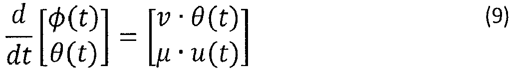
- a vehicle following a trajectory defined by (1) has heading ⁇ , curvature ⁇ , and curvature rate u .
- the vehicle's velocity is v .
- the problem to be solved is: Find a path that leads a vehicle onto a target line in the least amount of time, subject to constraints.
- Equation (2) and (3) represent initial conditions; equation (4) represents final conditions. Equation (5) represents the dynamics of the problem, while equation (6) is a constraint on curvature.
- heading may be restricted. For example, one may require that a vehicle approach a target line on a heading no greater than a maximum angle away from the line. In that case
- ⁇ f ⁇ 0 represents any desired final heading.
- Fig. 8 is a feedback map for the double integrator system subject to constraints given above.
- the feedback map shows two example trajectories in the ( ⁇ ⁇ , ⁇ ) plane. The first starts at A and ends at 0, while the second starts at E and ends at 0. Beginning at A, curvature ( ⁇ ) increases until the maximum curvature limit is reached at C. The curvature changes sign at B. From C to D the curvature is maximum and constant. The curvature decreases from D to 0. The second example trajectory starts at E and ends at 0. Beginning at E, curvature decreases until F. Curvature then increases until 0 is reached.
- the vehicle executes optimal turns.
- the optimal ( ⁇ ⁇ , ⁇ ) plane trajectories from A to 0 or from E to 0, of Fig. 8 leads to optimal turns in the (x, y) plane.
- the optimal ( ⁇ ⁇ , ⁇ ) plane trajectory from A to 0 leads to an optimal turn in the (x, y) plane constructed from clothoids (from A to B, B to C and D to 0) and a circular arc (from C to D).
- the optimal ( ⁇ ⁇ , ⁇ ) plane trajectory from E to 0 leads to an optimal turn in the (x, y) plane constructed from two clothoids (from E to F and F to 0).
- an optimal turn is defined as a path obtained by applying optimal double-integrator inputs (14) to continuous curvature equation (1).
- Optimal turns consist of: (i) a clothoid, (ii) a circular arc followed by a clothoid, (iii) a clothoid followed by a clothoid, or (iv) a clothoid followed by a circular arc followed by a clothoid.
- optimal turns guide a vehicle to a target configuration (e.g. zero heading and curvature) in minimum time.
- optimal turns may at least be used to create an efficient joining path from an initial configuration to a target configuration while obeying heading, curvature, curvature rate or other constraints.
- the approach described above may now be extended to account for cross track error.
- trajectories similar to those of Fig. 8 are plotted as a dark curve on the surface.
- Solution (22) or (24) may be used in feedback controller 505 in Fig. 5 .
- Fig. 10A shows an example path for a vehicle joining a straight line desired path while Fig. 10B shows u, ⁇ and ⁇ versus time for the path shown in Fig. 10A .
- the joining path is composed of clothoid 1010, circular arc 1015, clothoid 1020, straight line 1025, clothoid 1030, circular arc 1035 and clothoid 1040.
- Fig. 10A shows an example path for a vehicle joining a straight line desired path while Fig. 10B shows u, ⁇ and ⁇ versus time for the path shown in Fig. 10A .
- a joining path is shown that leads
- discontinuous line 1045 (for example) represents input u
- piecewise continuous line 1050 represents curvature ⁇
- smooth line 1055 represents heading ⁇
- dotted lines 1060 represent a curvature limit
- dot-dash lines 1065 represent a heading limit.
- An optimal solution for u has only three possible values: 1, 0 or -1.
- the slope of curvature ⁇ is flat during circular and straight line segments; the slope of ⁇ during clothoid segments reflects the maximum allowed steering angle rate. Heading 1055 varies smoothly; its maximum slope reflects the maximum allowed steering angle.
- Joining paths may be computed by solving (1) numerically and choosing u according to (22) or (24) at each time step.
- Joining paths computed by steps (1) - (5) above include one or more clothoids and may also include circular arcs and straight lines.
- An example joining path structure is: clothoid-line-clothoid-arc-clothoid. 22 other combinations of clothoids, arcs and lines are possible.
- a joining path from an arbitrary initial condition to a target line consists of: (i) an optimal turn, (ii) a line followed by an optimal turn, (iii) an optimal turn followed by an optimal turn, or (iv) an optimal turn followed by a line followed by an optimal turn. Note that the line specified in steps (2) and (3) may have zero length in which case one optimal turn is followed directly by another.
- Fig. 11 shows two example joining paths.
- x-axis 1105 is the target line.
- the longer joining path consists of an optimal turn 1110 to heading ⁇ ⁇ 4 , a straight line 1115, and an optimal turn 1120 onto the target line.
- the shorter path shows how, following steps (4) and (5) above, an optimal turn 1125 to heading ⁇ ⁇ 4 got cut off at y and an optimal turn 1130 to the target line was added from that point.
- ⁇ ⁇ 4 is a maximum allowed approach heading ( ⁇ max ) specified by a vehicle owner or operator.
- Joining paths may be computed using the integral approach by the path joining planner of Figs. 6 and 7 .
- An alternative approach to computing joining paths is based on consideration of curvature versus time (or distance) diagrams such as those shown in Figs. 12 and 13 .
- a turn toward a target line is initiated and allowed to progress for a certain amount of time.
- the consequences of the turn are then computed, the consequences being whether or not a turn in the opposite direction can be constructed that results in a trajectory that ends on the target line with zero heading and curvature. If a satisfactory turn is not achieved, the procedure is repeated with the initial turn allowed to progress for another time increment.
- This iterative approach is most conveniently implemented as code for a microprocessor. It does not readily admit to analytic solution, unlike the integral approach.
- Fig. 12 is a first diagram of curvature versus time or distance used in an iterative path planning method.
- time is used as the abscissa; speed is assumed constant, so distance could be used instead.
- the situation depicted is one in which an initial, positive turn has been allowed to progress until point B, at which point the turn is unwound in the opposite direction.
- Steering angle limits are included in the curvature limit ⁇ max as steering angle and curvature are related by wheelbase in a truck-like vehicle and by similar parameters in other vehicle types.
- Steering angle rate limits are included in the maximum slope of ⁇ (t).
- the shaded area under the ⁇ (t) curve i.e. the time integral of ⁇ (t) is proportional to heading change; see also (20) above.
- the sum of the initial heading ⁇ i , the accumulated positive heading change (shaded area denoted "+”), and the accumulated negative heading change (shaded area denoted "-") equals zero.
- Fig. 13 is a second diagram of curvature versus time or distance used in an iterative path planning method.
- Fig. 13 is similar to Fig. 12 .
- the initial curvature is not zero so the starting condition is ( ⁇ i ⁇ 0, ⁇ i , y i ).
- the curvature does not reach ⁇ max , but heading does reach its maximum and this leads to the zero curvature (constant heading) line before point B.
- the iterative method does not provide a mechanism to decide a priori whether an initial positive or negative (i.e. left or right) turn leads to a shorter joining path.
- Results obtained from an initial positive turn from a given starting condition may be compared to results obtained from an initial negative turn from the same condition. Whichever initial turn leads to the shorter joining path may then be used in practice.
- Fig. 14 is an example graph of final cross track error versus iteration number. As illustrated in Fig. 14 , the final cross track error, y f , may initially increase with further iterations of point B. However, once the cross track error becomes a decreasing function of B iteration number, an estimate of how far B must be incremented to achieve acceptable final cross track error may be obtained without trying every intermediate B iteration. Gradient descent methods may be used to estimate the optimum B, for example.
- Paths generated with the iterative method may be used in the path joining planner of Figs. 6 and 7 .
- Joining paths computed by either the integral or iterative approach may be used in advanced maneuvers. Velocity depending constraints may be included. Either approach may be extended to join desired paths that are not straight lines. Finally, non-optimal joining paths may sometimes be desirable.
- a 180 degree turn is an example of a path planning maneuver that has particular applicability in farming. Plowing, fertilizer, seeding and other operations are often performed along a set of parallel rows spanning a field. Upon reaching the end of a row, a farm vehicle turns around and joins the next row. A path planning autopilot can create a joining path from one row to another using the integral or iterative approaches described above.
- Figs. 15A- 15D illustrate turn-around paths.
- a curved joining path connects two straight line paths, e.g. field rows.
- the joining path has been computed using methods described above.
- the straight line paths are farther apart so the joining path includes a perpendicular, straight line section.
- Fig. 15C the straight line paths are too close to be joined without overshoot. This path may be followed in either direction so that the overshoot crosses either the starting or ending straight line as desired.
- Fig 15D the joining path overshoots both straight line paths equally.
- Figs. 15A - 15D Once any of the joining paths of Figs. 15A - 15D are computed, the distance required for the path in the x direction is known. This information may be used to start the turnaround at an appropriate point such that a vehicle (or an implement towed by it) stays within a boundary as shown in Fig. 3
- Turnarounds are an illustrative example of the utility of path planning. There is, of course, no requirement that the straight lines to be joined are parallel.
- the path planning approaches described above are general and accommodate any initial cross track error, heading and steering angle condition.
- Figs. 16A and 16B illustrate speed dependent curvature and curvature rate limits.
- curvature ⁇ and curvature rate d ⁇ /dt are plotted as solid curves versus velocity v. These curves show an example of how an autopilot may be tuned. As vehicle speed increases, curvature and curvature rate decrease. Dashed lines ("max") represent maximum limits in each figure. The shape of the curvature and curvature rate versus velocity curves may be adjusted to suit vehicle operator or autopilot manufacturer preferences.
- Curvature vs. velocity and curvature rate vs. velocity may be tuned in several different ways.
- One way is to drive a vehicle through a series of test maneuvers to discover the vehicle's maximum capabilities at various speeds.
- the autopilot may record a path followed by the vehicle, including speed, and derive maximum curvature and curvature rate from recorded data.
- a second way is for the autopilot to accept user input to specify a certain make and model of vehicle with known capabilities.
- a third way is to ask a vehicle operator to drive the vehicle as aggressively as he would ever want the autopilot to drive it.
- the autopilot may then record a path followed by the vehicle while the operator is driving and use recorded data to derive maximum operator-desired curvature and curvature rate.
- Some operators do not realize the full turning capabilities of their vehicles. Matching autopilot performance to operator comfort level helps prevent frightening the operator when he lets the autopilot take over vehicle control.
- Fig. 17 illustrates an approach to a curved desired path.
- Fig. 17 fixes 1705 and 1710 are indicated by triangles.
- Curve 1715 is the desired path to be joined.
- the tangent to the desired path closest to fix 1705 is labeled "1" while the tangent to the desired path closest to fix 1710 is labeled "2".
- Dashed lines connect each fix to their respective tangent.
- Curve 1720 is a joining path from the first fix to the first tangent "1”
- curve 1725 is a joining path from the second fix to the second tangent "2". Dotted curves on either side of curved path 1715 indicate maximum cross track error considered "close" to the curved path.
- a vehicle closer to the curved path than either of these two dotted curves may be guided onto the curved path with a small signal feedback autopilot.
- a large signal, feed-forward autopilot e.g. based on path planning techniques, may be used.
- Constructing a joining path to curved desired path 1715 proceeds as follows. Starting at fix 1705, tangent "1" to the nearest point on curve 1715 is computed. Path planning techniques, such as integral or iterative approaches, are used to compute joining path 1720 to tangent "1". Upon reaching fix 1710, tangent "2" to the now nearest point on curve 1715 is computed. Path planning techniques are used to compute joining path 1725 to tangent "2". This process may be repeated as many times as needed to construct a smooth joining path.
- When or how often to recalculate a new tangent to the current nearest point on the curved desired path may be decided based on how far away from the path the vehicle starts and/or the degree of curvature of the path.
- a new tangent may also be calculated at regular intervals regardless of distance or path curvature.
- a path planning autopilot may take this into account.
- a path planning autopilot may compute a joining path for the current speed and also a higher speed. If currently operating at 50% of the maximum vehicle speed, for example, an additional path appropriate for 90% of the maximum vehicle speed may also be computed. This way the autopilot can provide a margin in case the vehicle operator decides to speed up. Anticipating higher speeds helps prevent becoming stuck in maneuvers that lead to undesirable high-speed joining paths.
- a path planning autopilot may also be restricted by specifying the maximum curvature rate ⁇ to be less than that prescribed by vehicle absolute limits. Smaller values of ⁇ lead to less sharp turns. Paths may be recalculated whenever heading, curvature or curvature rate limits change.
- FIGs. 18A and 18B illustrate joining paths that are not necessarily optimal.
- a joining path starts from approximately (0, -1.8); in Fig. 18B , a joining path starts from approximately (0, 4).
- the joining path in Fig. 18A is one that maintains initial heading until getting close enough to the target line (e.g. reaching y ) to begin an optimal final turn. This path is not necessarily optimal because a steeper approach to the target line may be allowed.
- the joining path in Fig. 18B is one that maintains initial curvature until getting close enough to the target line (e.g. reaching y ) to begin an optimal final turn. This path is not necessarily optimal because a greater curvature may be allowed.
- the joining paths of Figs. 18A and 18B begin with a (possibly) non-optimal and end with an optimal final turn.
- Non-optimal paths such as those illustrated in Figs. 18A and 18B may be desirable from the point of view of operator comfort. In both cases, the non-optimal paths begin by guiding the vehicle to continue doing what it is already doing: no heading change in the case Fig. 18A ; no steering angle change in the case of Fig. 18B . This behavior provides a smooth, non-startling transition from operator control to autopilot control of a vehicle. Of course, strategies that lead to non-optimal paths are not desirable if the vehicle does not eventually reach a position (e.g. y ) from which an optimal final turn may be made. Maintaining an initial heading, for example, does not work if that heading takes the vehicle away from the target path.
- a position e.g. y
- a path planning autopilot and methods for computing joining paths have been described.
- the autopilot provides efficient vehicle guidance even when a vehicle is far from a desired path.
- the autopilot also offers direct control over parameters such as steering angle rate without relying on heuristic limits.
Landscapes
- Engineering & Computer Science (AREA)
- Mechanical Engineering (AREA)
- Remote Sensing (AREA)
- Radar, Positioning & Navigation (AREA)
- Life Sciences & Earth Sciences (AREA)
- Transportation (AREA)
- Chemical & Material Sciences (AREA)
- Combustion & Propulsion (AREA)
- Aviation & Aerospace Engineering (AREA)
- Physics & Mathematics (AREA)
- General Physics & Mathematics (AREA)
- Automation & Control Theory (AREA)
- Soil Sciences (AREA)
- Environmental Sciences (AREA)
- Control Of Position, Course, Altitude, Or Attitude Of Moving Bodies (AREA)
Description
- The disclosure is generally related to automatic control systems for vehicles.
- Guiding a farm tractor, construction vehicle, mining truck, army tank or other large vehicle according to a precise, desired path often saves time and energy compared to sloppy operating. Precise farm tractor control, for example, benefits farmers, consumers and society as a whole. Farmers are able to work more efficiently, and spend less money on fertilizers and pesticides. Consumers enjoy lower prices for high quality produce, and precise use of farm land and farm chemicals reduces waste and excess runoff.
- Autopilot systems that guide farm tractors, spray trucks, harvesters and the like with high accuracy and repeatability contribute to efficient land and chemical use. For example, fields are often sprayed with booms 90-feet-wide or even larger. When using such a wide boom it would seem prudent to allow a few feet of overlap from one spray swath to the next. However, the overlap may be reduced to just inches if the tractor or spray truck is equipped with a high performance autopilot. The savings accrued from not double-spraying swath edges add up quickly on large area farms.
- Existing autopilot systems are adequate for keeping vehicles on a predefined path. These autopilots are based on feedback control techniques and they can make a large farm tractor, for example, follow a line within one or two inches cross-track error.
Fig. 1A shows a vehicle following a path under feedback control;vehicle 105 followspath 110. When the cross track error, XTE, is smaller than the vehicle wheelbase, b, the vehicle is in a small signal regime or "close" to the desired path. - Feedback autopilots do not perform as well when a vehicle is far off from a desired path. Common situations where this occurs include joining a path from far away or turning around at the end of a path to join a nearby path.
Fig. 1B shows a vehicle with apossible path 125 that could result from using a small-signal feedback autopilot in a large-signal regime.Vehicle 115 is guided by a feedback autopilot towardpath 120. When the cross track error is larger than the vehicle wheelbase, the vehicle is in the large signal regime or "far" from the desired path. - With conventional feedback autopilots, tradeoffs exist between performance in the small signal regime and acceptable behavior in the large signal regime. For example, high feedback gain that keeps cross track error small in the small signal regime may result in steep approaches to a desired path and oscillation when joining the path as shown in
Fig. 1B . Conventional autopilots avoid undesirable large-signal behavior by invoking heuristic limits when large deviations from a desired path are encountered. These limits mean that large-signal guidance is not as efficient as it could be. - In the examples above wheelbase is used as an example of a characteristic length scale to divide small and large signal regimes. Other characteristic lengths may be used; e.g. distance travelled in a characteristic autopilot response time. More generally, the small signal regime refers to any situation where a vehicle autopilot behaves as a linear, time-invariant system. The large signal regime, on the other hand refers to situations where nonlinear behavior, such as steering angle limits or steering angle rate limits, occurs.
- What is needed is a vehicle autopilot that offers high performance guidance regardless of whether a vehicle is near or far from a desired path. The autopilot should not only keep a vehicle on a path, but also guide it efficiently to join a path from any starting point.
-
US 2009/099730 discloses a method for steering an agricultural vehicle comprising: receiving global positioning system (GPS) data including position and velocity information corresponding to at least one of a position, velocity, and course of the vehicle; receiving a yaw rate signal; and computing a compensated heading, the compensated heading comprising a blend of the yaw rate signal with heading information based on the GPS data. For each desired swath comprising a plurality of desired positions and desired headings, the method also comprises: computing an actual track and a cross track error from the desired swath based on the compensated heading and the position; calculating a desired radius of curvature to arrive at the desired track with a desired heading; and generating a steering command based on the desired radius of curvature to a steering mechanism, the steering mechanism configured to direct the vehicle. -
US 2009/118904 discloses methods and systems for planning the path of an agricultural vehicle. In one embodiment, a first point of a first planned path and a second point of a second planned path are determined. A path plan is then automatically generated connecting the first point and the second point. -
US 2007/021913 discloses an adaptive guidance system for a vehicle that includes an on-board GPS receiver, an on-board processor adapted to store a preplanned guide pattern and a guidance device. The processor includes a comparison function for comparing the vehicle GPS position with a line segment of the preplanned guide pattern. The processor controls the guidance device for guiding the vehicle along the line segment. Various guide pattern modification functions are programmed into the processor, including best-fit polynomial correction, spline correction, turn-flattening to accommodate minimum vehicle turning radii and automatic end-of-swath keyhole turning. -
US 2010/204866 discloses a method for determining a vehicle path for autonomously parallel parking a vehicle in a space between a first object and a second object. A distance is remotely sensed between the first object and the second object. A determination is made whether the distance is sufficient to parallel park the vehicle between. A first position to initiate a parallel parking maneuver is determined. A second position within the available parking space corresponding to an end position of the vehicle path is determined. A first arc shaped trajectory of travel is determined between the first position and an intermediate position, and a second arc shaped trajectory of travel is determined between the second position and the intermediate position.; The first arc shaped trajectory is complementary to the second arc shaped trajectory for forming a clothoid which provides a smoothed rearward steering maneuver between the first position to the second position. -
-
Fig. 1A shows a vehicle following a path under feedback control. -
Fig. 1B shows a vehicle with a possible path that could result from using a small-signal feedback autopilot in a large-signal regime. -
Fig. 2A shows a vehicle characterized by an arbitrary position (x, y), heading (φ), and curvature (θ); and a desired path for the vehicle to follow. -
Fig. 2B shows a vehicle following a planned path to join a desired path. -
Fig. 3 shows a turn-around path planned for a tractor towing an implement inside a field boundary. -
Fig. 4 is a block diagram of a path planning autopilot including feedback and feed-forward controllers. -
Fig. 5 is a block diagram of a feedback control system based on path planning algorithms. -
Fig. 6 is a block diagram of a feedback and feed-forward control system in feedback mode. -
Fig. 7 is a block diagram of a feedback and feed-forward control system in combined feedback and feed-forward mode. -
Fig. 8 is a feedback map for a double integrator system subject to constraints. -
Fig. 9 is a plot of a surface representing cross track distance travelled during turns from all possible initial conditions of heading and curvature subject to constraints. -
Fig. 10A shows an example path for a vehicle joining a straight line desired path. -
Fig. 10B shows u, θ and φ versus time for the path shown inFig. 10A . -
Fig. 11 shows two example joining paths. -
Fig. 12 is a first diagram of curvature versus time or distance used in an iterative path planning method. -
Fig. 13 is a second diagram of curvature versus time or distance used in an iterative path planning method. -
Fig. 14 is an example graph of final cross track error versus iteration number in an iterative path planning method. -
Figs. 15A - 15D illustrate turn-around paths. -
Figs. 16A and 16B illustrate speed dependent curvature and curvature rate limits. -
Fig. 17 illustrates an approach to a curved desired path. -
Figs. 18A and 18B illustrate joining paths that are not necessarily optimal. - The scope of the invention is defined in the appended claims. The embodiments described in the description are merely exemplary and are intended to be illustrative. path planning autopilot described below provides more sophisticated vehicle guidance than is possible with a conventional autopilot.
Fig. 2A shows avehicle 205 in a configuration defined by an arbitrary position (x, y), heading (φ), and curvature (θ); and a desiredpath 210 for the vehicle to follow. A path planning autopilot creates an efficient joining path that takes the vehicle from an arbitrary initial configuration (y, φ, θ) to a desired path. The initial configuration may be near or far from the desired path. As an example,Fig. 2B shows avehicle 215 following aplanned path 220 to join a desiredpath 225. - Unlike conventional autopilots, a path planning autopilot offers direct control over constraints such as maximum permitted steering angle or maximum steering angle rate. Such constraints may be specified as functions of vehicle speed. Path planning techniques may be implemented as a complementary feed-forward capability of a feedback autopilot or they may replace feedback all together.
- Many advanced maneuvers are possible with a path planning autopilot. Paths may be joined at up to specified maximum angles such as α, the angle between
dotted line 230 and desiredpath 225 inFig. 2B . A desired path may be joined in a specified direction, a capability that is used in turn-arounds.Fig. 3 shows a turn-around path planned for atractor 305 towing an implement 310 inside afield boundary 315.Planned path 320 is designed to keep implement 310 more than an implement half-width, W, from the boundary.Planned path 320 joins desiredpath 325 in a direction opposite to the tractor's present heading. - A path planning autopilot calculates an efficient path for a vehicle to follow. The autopilot guides the vehicle along this path using a pure feedback or a combined feed-forward and feedback control architecture. Two different approaches for calculating efficient paths are described.
- A typical scenario that illustrates the utility of a path planning autopilot is joining a desired path. In farming, for example, a tractor operator may wish to join predefined, straight line for planting, spraying or harvesting. There is no requirement to join the line at any particular position. Rather, the operator would simply like to join the line in the least time within constraints of comfortable operation.
- The joining path that guides a vehicle from its initial position to a desired line has continuous curvature, restricted to be less than a maximum curvature limit. This means that the joining path has no sharp corners and takes into account practical limits on how fast a vehicle can change its curvature and heading.
- For wheeled vehicles, curvature is determined by wheel steering angle and wheelbase. Path planning autopilots may be used with truck-like vehicles having two steerable wheels and two or more fixed wheels, center hinge vehicles, tracked vehicles, tricycle vehicles, etc. Some vehicle control systems accept curvature as a direct input rather than steering angle.
- Joining paths are calculated assuming constant vehicle speed. Joining paths may be recalculated whenever speed changes or they may be recalculated periodically regardless of whether or not vehicle speed has changed.
- Joining paths are constructed as a series of straight line, circular and clothoid segments. Clothoids are used to join segments of different, constant curvature; e.g. to join a line and a circular arc. The curvature of a clothoid changes linearly with curve length. Clothoids are also called Euler spirals or Cornu spirals. Reasonable approximations to clothoids may also be used.
-
Fig. 4 is a block diagram of a path planning autopilot including feedback and feed-forward controllers. The autopilot includes amain unit 405 having a feedback controller, a feed-forward controller, a processor and memory. Functional blocks of the main unit may be implemented with general purpose microprocessors, application-specific integrated circuits, or a combination of the two. - The main unit receives input from GNSS (global navigational satellite system)
receiver 410 andsensors 415. The main unit sends output to actuators 420.GNSS receiver 410 may use signals from any combination of Global Positioning System, Glonass, Beidou/Compass or similar satellite constellations. The receiver may use differential corrections provided by the Wide Area Augmentation System and/or real-time kinematic positioning techniques to improve accuracy. The receiver provides the main unit with regular position, velocity and time updates. -
Sensors 415 include steering sensors that report vehicle steering angle and heading sensors that report vehicle heading to the main unit. Heading may be sensed from a combination of GNSS and inertial measurements. Steering angle may be sensed by a mechanical sensor placed on a steering linkage or by inertial measurements of a steering linkage.Sensors 415 may also be omitted if heading and curvature of vehicle track are estimated from GNSS measurements alone. -
Actuators 420 include a steering actuator to steer a vehicle. A steering actuator may turn a vehicle's steering wheel or tiller, or it may control a steering mechanism directly. On some vehicles steering actuators operate hydraulic valves to control steering linkages without moving the operator's steering wheel. - A path planning autopilot may include many other functions, sensors and actuators. For simplicity, only some of those pertinent to path planning operations have been included in
Fig. 4 . A display and user input devices are examples of components omitted fromFig. 4 . User input may be necessary for system tuning, for example. The system ofFig. 4 may operate in different modes, three of which are illustrated inFigs. 5 ,6 and7 . - A path planning autopilot may use path planning techniques in a feedback control system or it may use path planning in a combined feedback / feed-forward control system.
Fig. 5 is a block diagram of a feedback control system based on path planning algorithms. InFig. 5 ,feedback controller 505controls vehicle 510 by sending curvature rate (u) or curvature (θ) command signals to it. Actual vehicle heading (φ) and cross track error (y) as measured by a GNSS receiver, heading sensor and/or other sensors are combined with desired curvature, heading and track (θ, φ, y) to form an error signal forcontroller 505. - The method used by
controller 505 to determine u or θ is described in detail below. At this point suffice it to say that the controller repeatedly calculates a joining path to guide the vehicle from its present position to a desired path, and generates control commands that cause the vehicle to follow the joining path. The controller is not based on conventional proportional-integral-derivative (PID) techniques. -
Figs. 6 and7 are block diagrams of a feedback and feed-forward control system in feedback, and combined feedback and feed-forward modes, respectively. InFigs. 6 and7 ,feedback controller 605controls vehicle 610 by sending curvature (θ) commands to it. (Alternatively,feedback controller 615 may send curvature rate (u) commands to the vehicle.) Actual vehicle heading (φ) and cross track error (y) as measured by a GNSS receiver, heading sensor and/or other sensors are combined with parameters of a desiredpath 620 to form an error signal forcontroller 605.Feedback controller 605 may be a conventional PID controller unlikefeedback controller 505. - In
Figs. 6 and7 , solid arrows represent active signal paths, while dashed arrows represent signal paths that are turned off. Thus inFig. 6 , feedback controller uses an error signal derived from the difference between measured and desired paths to generate feedback control signal θFB. This mode may be used when the vehicle is close to the desired path. - When the vehicle is far from a desired path, the control system switches to the mode illustrated in
Fig. 7 . A typical scenario in which a vehicle is far from a desired path is when an autopilot system is engaged before the vehicle is established on the path. A set of parallel swaths may have been created to guide a tractor over a farm field, for example, and the tractor operator may want the autopilot to guide the tractor to the nearest one. When this happens,path joining planner 615 calculates an efficient path from the vehicle's present position to the desired path. -
Path joining planner 615 calculates a joining path to guide the vehicle to the desired path and provides a feed-forward control signal, θFF, which is combined with feedback control signal θFB to guidevehicle 610. For purposes offeedback controller 605, the joining path is the desired path until the original desiredpath 620 is reached. Thus feedback reference signal (φ, y) is derived from the path joining planner during that time. The path joining planner is the feed-forward mechanism described in connection withFig. 4 . Methods used by the feed-forward, path joining planner are described in detail below. - Alternatively, once
path joining planner 615 calculates a joining path, that joining path continuing onto the original desired path (from the point where the joining path meets the original path) may become the new desired path. The original desired path before the point where the joining path meets it may then be discarded. - Autopilots having a path-planning, feedback and feed-forward control system like that of
Figs. 6 and7 may use a switch to alternate between modes. The mode is selected based on vehicle distance from desiredpath 620; near the path feedback control is used, far from it combined feed-forward and feedback control is used. Criteria to determine "near" and "far" may be based on characteristic lengths such as vehicle wheelbase or distance travelled in a characteristic response time, or whether or not steering angle or steering angle rate limits are encountered. - Alternatively, a control system may operate in the mode illustrated in
Fig. 7 continuously. When the vehicle is near the desired (620) path, output signals from the path joining planner are small and may have negligible practical influence on the feedback control system. Thus, the path joining planner may be kept online all the time. -
Figs. 5 - 7 show measured (φ y) data being combined with desired path data and then sent tofeedback controller - Two different approaches for calculating efficient joining paths are described in detail below: an integral approach and an iterative approach. Each approach is first described in terms of planning paths to join the straight line y = 0. Extensions to joining curves are discussed later. Symbols used in the discussion below are defined in Table 1.
Table 1: Symbol definitions. (x, y) position φ heading θ curvature u curvature rate - The time evolution of a continuous curvature trajectory in the x -y plane is described by:

- A vehicle following a trajectory defined by (1) has heading φ, curvature θ, and curvature rate u. The vehicle's velocity is v.
- The problem to be solved is: Find a path that leads a vehicle onto a target line in the least amount of time, subject to constraints. The target line to be joined is the x axis (y = 0) and x position may be dropped from consideration entirely. Since (1) is invariant with respect to time, the initial time may be set to t = 0.
- A formal statement of the optimal control problem is: Find a piecewise continuous solution for u for all times from t = 0 to t = tf such that constraints (2) - (6) below are met and the final time, tf, is minimized.


- Here θ max is the maximum allowed curvature and µ is the maximum allowed rate of change of curvature. µ normalizes u such that|u| ≤ 1. (Note: µ > 0) Equations (2) and (3) represent initial conditions; equation (4) represents final conditions. Equation (5) represents the dynamics of the problem, while equation (6) is a constraint on curvature.
- Physically, φ = φ ± n · 2π, so φf = n · 2π where n is an integer. In some cases, heading may be restricted. For example, one may require that a vehicle approach a target line on a heading no greater than a maximum angle away from the line. In that case |φ(t)| ≤ φmax where 0 < φmax ≤ π.
- The problem just described is complicated. Rather than solve it directly, it is easier to consider a simpler problem: Calculate a path that leads a vehicle from its initial heading and curvature to some desired final heading and zero curvature. In other words, ignore the y coordinate or cross track error. The statement of the control problem now becomes: Find a piecewise continuous solution for u (-1 ≤ u ≤ 1)for all times from t = 0 to t = tf such that constraints (7) - (10) below are met and the final time, tf, is minimized.


- Here φf ≠ 0 represents any desired final heading.
- This problem is an example of the so-called "double integrator" problem, solutions to which are well known. The optimal input, u(t), is 0, 1 or -1 depending on the values of φ and θ. Let Δφ = φ - φf and


- The optimal input, u(t) =
u (Δφ(t), θ(t)) is then: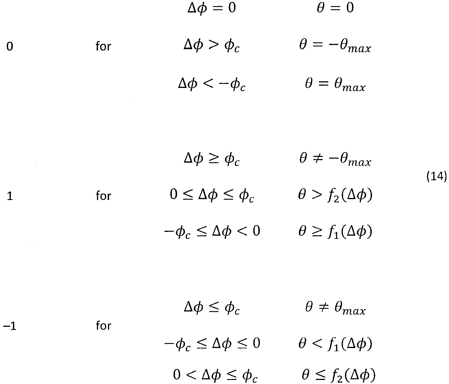
-
Fig. 8 is a feedback map for the double integrator system subject to constraints given above. The feedback map shows two example trajectories in the (Δφ, θ) plane. The first starts at A and ends at 0, while the second starts at E and ends at 0. Beginning at A, curvature (θ) increases until the maximum curvature limit is reached at C. The curvature changes sign at B. From C to D the curvature is maximum and constant. The curvature decreases from D to 0. The second example trajectory starts at E and ends at 0. Beginning at E, curvature decreases until F. Curvature then increases until 0 is reached. - When optimal inputs (14) are applied to a vehicle obeying equation (1), the vehicle executes optimal turns. Following the optimal (Δφ, θ) plane trajectories, from A to 0 or from E to 0, of
Fig. 8 leads to optimal turns in the (x, y) plane. The optimal (Δφ, θ) plane trajectory from A to 0 leads to an optimal turn in the (x, y) plane constructed from clothoids (from A to B, B to C and D to 0) and a circular arc (from C to D). The optimal (Δφ, θ) plane trajectory from E to 0 leads to an optimal turn in the (x, y) plane constructed from two clothoids (from E to F and F to 0). - Thus, an optimal turn is defined as a path obtained by applying optimal double-integrator inputs (14) to continuous curvature equation (1). Optimal turns consist of: (i) a clothoid, (ii) a circular arc followed by a clothoid, (iii) a clothoid followed by a clothoid, or (iv) a clothoid followed by a circular arc followed by a clothoid. In theory optimal turns guide a vehicle to a target configuration (e.g. zero heading and curvature) in minimum time. In practice optimal turns may at least be used to create an efficient joining path from an initial configuration to a target configuration while obeying heading, curvature, curvature rate or other constraints.
- The approach described above may now be extended to account for cross track error. The control problem statement becomes: Find a piecewise continuous solution for u (-1 ≤ u ≤ 1)for all times from t = 0 to t = tf such that constraints (15) - (18) below are met and the final time, tf, is minimized.


- The target line is the x-axis and φf = 0. This problem and its solutions are invariant with respect to y so any trajectory may be shifted in y such that yf = 0. Equivalently, if y0 is picked correctly, then yf = 0. That value of y0 that results in yf = 0 is defined as
y (φ 0 , θ 0). - Or, said another way: starting from initial conditions of heading, curvature and cross track error (φ0, θ0, y0), an optimal turn to zero heading and zero curvature will end on the x-axis if y 0 =
y (φ 0 , θ 0).y is found by integrating ∫ y(t)dt backwards until a desired heading and curvature are reached for all permissible values of φ and θ:


-
Fig. 9 is a plot of y =y (φ, θ) for all allowed φ and θ. InFig. 9 , v = 1, µ = 0.6 and θmax = 50 degrees. All solutions for y(tf ) = φ(tf ) = θ(tf ) = 0 lie on the y =y (φ, θ) surface plotted. In particular, trajectories similar to those ofFig. 8 are plotted as a dark curve on the surface. - The solution of the whole problem, including cross track error, may now be specified for two cases: with and without heading constraints. When there are no heading constraints:

- Solution (22) prescribes an optimal turn onto the target line if y(t) =
y (φ, θ). If y(t) ≠y (φ, θ) then an optimal turn is made toward a line perpendicular to the target line; i.e. to a line heading

- When heading constraints are present:

- Solution (24) prescribes an optimal turn onto the target line if y(t) =
y (φ, θ). If y(t) ≠y (φ θ) then an optimal turn is made toward a line inclined at an angle min(φmax, π/2) to the target line. (min(x, y) equals x or y, whichever is least.) The turn toward the line, or subsequent travel along it, yields a trajectory that intersects with
- Solution (22) or (24) may be used in
feedback controller 505 inFig. 5 . -
Fig. 10A shows an example path for a vehicle joining a straight line desired path whileFig. 10B shows u, θ and φ versus time for the path shown inFig. 10A . InFig. 10A , x-axis (y = 0) 1005 is the target line to be joined. A joining path is shown that leads a vehicle from an initial condition (y0 = 2.5, φ0= 0.3, θ0 = 0) to the target line. The joining path is composed ofclothoid 1010,circular arc 1015,clothoid 1020,straight line 1025,clothoid 1030,circular arc 1035 andclothoid 1040. InFig. 10B , discontinuous line 1045 (for example) represents input u, piecewisecontinuous line 1050 represents curvature θ,smooth line 1055 represents heading φ, dottedlines 1060 represent a curvature limit, and dot-dash lines 1065 represent a heading limit. An optimal solution for u has only three possible values: 1, 0 or -1. The slope of curvature θ is flat during circular and straight line segments; the slope of θ during clothoid segments reflects the maximum allowed steering angle rate. Heading 1055 varies smoothly; its maximum slope reflects the maximum allowed steering angle. - Joining paths may be computed by solving (1) numerically and choosing u according to (22) or (24) at each time step. Alternatively (19), (20) and (21) may be integrated analytically and the x coordinate may be found from:

- The following steps may be used to compute joining paths to target lines starting from an initial vehicle configuration [y 0 φ 0 θ 0]:
- (1)
- (a) If y 0 =
y (φ 0, θ 0), then go to step (5). - (b) If y 0 ≠
y (φ 0, θ 0) and φ 0 = -sgn(φ 0) · φmax (or
- (c) Otherwise, continue to step (2).
- (a) If y 0 =
- (2) Compute an optimal turn onto a line inclined at an angle to the target line by ±φmax or
- (a) If y(t 1) =
y (φ(t 1), θ(t 1)), then go to step (5). - (b) If y 0 ≷
y (φ 0, θ 0) and y(t 1) ≶y (φ(t 1), θ(t 1)), then go to step (4). - (c) Otherwise, continue to step (3).
- (a) If y(t 1) =
- (3) Add a straight line until time t3 where t3 satisfies y(t 3) =
y (φ(t 3), θ(t 3)). Go to step (5). - (4) Find t2, t 0 < t 2 < t 1, where t2 satisfies y(t 2) =
y (φ(t 2), θ(t 2)). Discard the trajectory computed so far for all times t > t2. Continue to step (5). - (5) Compute an optimal turn onto the target line.
- Expressed without mathematical symbols these steps are, starting from any initial vehicle cross track error, heading and steering angle:
- (1)
- (a) If the vehicle is at the right distance away from the target line to start the final turn, then go to step (5).
- (b) if not, and if the heading is at the maximum allowed angle to the target line (or perpendicular to the target line) then go to step (3).
- (c) Otherwise, continue to step (2).
- (2) Compute an optimal turn onto a line inclined at the maximum allowed angle to the target line or perpendicular to it.
- (d) If this turn ends at the right distance away from the target line to start the final turn, then go to step (5).
- (e) If, at some point during this turn, the right distance away from the target line to start the final turn is reached, then go to step (4).
- (f) Otherwise, continue to step (3).
- (3) Add a straight line proceeding in the direction of the current heading ending at the right distance away from the target line to start the final turn; then go to step (5).
- (4) Find the point at which the right distance was reached. Continuing from this point, go to step (5).
- (5) Compute an optimal turn onto the target line.
- Joining paths computed by steps (1) - (5) above include one or more clothoids and may also include circular arcs and straight lines. An example joining path structure is: clothoid-line-clothoid-arc-clothoid. 22 other combinations of clothoids, arcs and lines are possible. In general, a joining path from an arbitrary initial condition to a target line consists of: (i) an optimal turn, (ii) a line followed by an optimal turn, (iii) an optimal turn followed by an optimal turn, or (iv) an optimal turn followed by a line followed by an optimal turn. Note that the line specified in steps (2) and (3) may have zero length in which case one optimal turn is followed directly by another.
-
Fig. 11 shows two example joining paths. InFig. 11 ,x-axis 1105 is the target line. The longer joining path consists of anoptimal turn 1110 to heading
straight line 1115, and anoptimal turn 1120 onto the target line. The shorter path shows how, following steps (4) and (5) above, anoptimal turn 1125 to heading
y and anoptimal turn 1130 to the target line was added from that point. In both cases
- Note that for the shorter path in
Fig. 11 , and other paths like it, instead of computing a complete turn according to step (2) and then finding where it crossesy according to step (4), one could check ify is reached at each point in as the turn is computed. Other, small procedural variations are no doubt possible. - Joining paths may be computed using the integral approach by the path joining planner of
Figs. 6 and7 . - An alternative approach to computing joining paths is based on consideration of curvature versus time (or distance) diagrams such as those shown in
Figs. 12 and13 . In this approach a turn toward a target line is initiated and allowed to progress for a certain amount of time. The consequences of the turn are then computed, the consequences being whether or not a turn in the opposite direction can be constructed that results in a trajectory that ends on the target line with zero heading and curvature. If a satisfactory turn is not achieved, the procedure is repeated with the initial turn allowed to progress for another time increment. This iterative approach is most conveniently implemented as code for a microprocessor. It does not readily admit to analytic solution, unlike the integral approach. -
Fig. 12 is a first diagram of curvature versus time or distance used in an iterative path planning method. InFig. 12 time is used as the abscissa; speed is assumed constant, so distance could be used instead. The situation depicted is one in which an initial, positive turn has been allowed to progress until point B, at which point the turn is unwound in the opposite direction. Steering angle limits are included in the curvature limit ±θmax as steering angle and curvature are related by wheelbase in a truck-like vehicle and by similar parameters in other vehicle types. Steering angle rate limits are included in the maximum slope of θ(t). The shaded area under the θ(t) curve (i.e. the time integral of θ(t)) is proportional to heading change; see also (20) above. - Considering
Fig. 12 now in detail: At time t = 0, curvature θ = 0, heading φ = φi, and cross track error y = yi. A positive turn is begun at maximum steering angle rate until θ reaches θmax. θ remains at θmax until point B. For each point B, the heading at point C is tested to see if it exceeds a maximum heading constraint. If it has, point B has been incremented too far and the previous increment must be used instead. InFig. 12 , a maximum heading constraint is not reached and curvature is steadily decreased from point B until it reaches the minimum limit, -θmax.Fig. 13 , discussed below, shows a case where a maximum heading limit is reached. - For each point B, the part of the diagram in
Fig. 12 representing negative curvature, i.e. the part to the right of point C is then constructed such that it has enough area to make the final heading φf = 0. In other words, the sum of the initial heading φi, the accumulated positive heading change (shaded area denoted "+"), and the accumulated negative heading change (shaded area denoted "-") equals zero. - Next the final cross track error yf is computed. If yf = 0, then the problem is solved; if not, then point B is incremented one time step and the procedure just outline is repeated.
-
Fig. 13 is a second diagram of curvature versus time or distance used in an iterative path planning method.Fig. 13 is similar toFig. 12 . InFig. 13 , however, the initial curvature is not zero so the starting condition is (θi ≠ 0, φi, yi). The curvature does not reach θmax, but heading does reach its maximum and this leads to the zero curvature (constant heading) line before point B. Point B is incremented in time until a negative turn can be constructed that results in the final condition (θf = 0, φr = 0, yf = 0). - The iterative method does not provide a mechanism to decide a priori whether an initial positive or negative (i.e. left or right) turn leads to a shorter joining path. Results obtained from an initial positive turn from a given starting condition may be compared to results obtained from an initial negative turn from the same condition. Whichever initial turn leads to the shorter joining path may then be used in practice.
- The iterative method proceeds until the final cross track error is zero or at least minimized to within a range that can be handled by a conventional feedback autopilot. Cross track error less than the vehicle wheelbase or some other characteristic length may be close enough.
Fig. 14 is an example graph of final cross track error versus iteration number. As illustrated inFig. 14 , the final cross track error, yf, may initially increase with further iterations of point B. However, once the cross track error becomes a decreasing function of B iteration number, an estimate of how far B must be incremented to achieve acceptable final cross track error may be obtained without trying every intermediate B iteration. Gradient descent methods may be used to estimate the optimum B, for example. - Paths generated with the iterative method may be used in the path joining planner of
Figs. 6 and7 . - Joining paths computed by either the integral or iterative approach may be used in advanced maneuvers. Velocity depending constraints may be included. Either approach may be extended to join desired paths that are not straight lines. Finally, non-optimal joining paths may sometimes be desirable.
- A 180 degree turn is an example of a path planning maneuver that has particular applicability in farming. Plowing, fertilizer, seeding and other operations are often performed along a set of parallel rows spanning a field. Upon reaching the end of a row, a farm vehicle turns around and joins the next row. A path planning autopilot can create a joining path from one row to another using the integral or iterative approaches described above.
-
Figs. 15A- 15D illustrate turn-around paths. In each ofFigs. 15A- 15D a curved joining path connects two straight line paths, e.g. field rows. The joining path has been computed using methods described above. InFig. 15A two straight line paths (y = 0 and y = 2) are just the right distance apart that a maximum curvature joining path connects them without overshoot. InFig. 15B the straight line paths are farther apart so the joining path includes a perpendicular, straight line section. InFig. 15C the straight line paths are too close to be joined without overshoot. This path may be followed in either direction so that the overshoot crosses either the starting or ending straight line as desired. InFig 15D the joining path overshoots both straight line paths equally. This joining path is constructed by starting at half way point where y = half the distance between straight line paths, φ = -π/2, and θ = θmax and computing a joining path to the line y = 0. This generates half of the joining path shown in the figure; the other half is just the mirror image. - Once any of the joining paths of
Figs. 15A - 15D are computed, the distance required for the path in the x direction is known. This information may be used to start the turnaround at an appropriate point such that a vehicle (or an implement towed by it) stays within a boundary as shown inFig. 3 - Turnarounds are an illustrative example of the utility of path planning. There is, of course, no requirement that the straight lines to be joined are parallel. The path planning approaches described above are general and accommodate any initial cross track error, heading and steering angle condition.
- The integral and iterative path planning approaches assume constant vehicle speed. If the speed changes, a new joining path may be computed to take the change into account. For any given vehicle speed maximum limits may be placed on parameters such as curvature and curvature rate. For a typical farm vehicle, these limits correspond to maximum allowed steering angle and steering angle rate.
Figs. 16A and 16B illustrate speed dependent curvature and curvature rate limits. - In
Figs. 16 and 16B , curvature θ and curvature rate dθ/dt, respectively, are plotted as solid curves versus velocity v. These curves show an example of how an autopilot may be tuned. As vehicle speed increases, curvature and curvature rate decrease. Dashed lines ("max") represent maximum limits in each figure. The shape of the curvature and curvature rate versus velocity curves may be adjusted to suit vehicle operator or autopilot manufacturer preferences. - Curvature vs. velocity and curvature rate vs. velocity may be tuned in several different ways. One way is to drive a vehicle through a series of test maneuvers to discover the vehicle's maximum capabilities at various speeds. The autopilot may record a path followed by the vehicle, including speed, and derive maximum curvature and curvature rate from recorded data. A second way is for the autopilot to accept user input to specify a certain make and model of vehicle with known capabilities. A third way is to ask a vehicle operator to drive the vehicle as aggressively as he would ever want the autopilot to drive it. The autopilot may then record a path followed by the vehicle while the operator is driving and use recorded data to derive maximum operator-desired curvature and curvature rate. Some operators do not realize the full turning capabilities of their vehicles. Matching autopilot performance to operator comfort level helps prevent frightening the operator when he lets the autopilot take over vehicle control.
- So far path planning techniques have been described in terms of creating joining paths to straight lines. It is also possible to join curved paths, however. The overall strategy for joining a curve is to use path planning to guide a vehicle close enough to the curve for feedback techniques to take over. First a joining path to the nearest tangent of the curve is created. As the joining path approaches the curve the nearest tangent changes; a new joining path to the new nearest tangent is then created. The process of creating and following joining paths to a nearest tangent may be repeated to construct an overall joining path that ends close enough to the curved path that feedback techniques may be used to guide a vehicle the rest of the way.
-
Fig. 17 illustrates an approach to a curved desired path.Fig. 17 fixes Curve 1715 is the desired path to be joined. The tangent to the desired path closest to fix 1705 is labeled "1" while the tangent to the desired path closest to fix 1710 is labeled "2". Dashed lines connect each fix to their respective tangent.Curve 1720 is a joining path from the first fix to the first tangent "1", whilecurve 1725 is a joining path from the second fix to the second tangent "2". Dotted curves on either side ofcurved path 1715 indicate maximum cross track error considered "close" to the curved path. A vehicle closer to the curved path than either of these two dotted curves may be guided onto the curved path with a small signal feedback autopilot. Farther away, a large signal, feed-forward autopilot, e.g. based on path planning techniques, may be used. - Constructing a joining path to curved desired
path 1715 proceeds as follows. Starting atfix 1705, tangent "1" to the nearest point oncurve 1715 is computed. Path planning techniques, such as integral or iterative approaches, are used to compute joiningpath 1720 to tangent "1". Upon reachingfix 1710, tangent "2" to the now nearest point oncurve 1715 is computed. Path planning techniques are used to compute joiningpath 1725 to tangent "2". This process may be repeated as many times as needed to construct a smooth joining path. - After the joining path has been calculated the vehicle follows it under the guidance of an autopilot such as described in connection with
Figs. 4 - 7 . Once the vehicle is close to the curved path it is guided the rest of the way by a feedback autopilot. Dashedcurve 1730 is the track that results from feedback guidance tocurve 1715. - When or how often to recalculate a new tangent to the current nearest point on the curved desired path may be decided based on how far away from the path the vehicle starts and/or the degree of curvature of the path. A new tangent may also be calculated at regular intervals regardless of distance or path curvature.
- As previously mentioned, vehicle speed changes, whether joining a curved or straight desired path, may be accommodated by recalculating a joining path. High-speed maneuvers take more space than low-speed maneuvers, however, and a path planning autopilot may take this into account. When planning a maneuver near a boundary, such as a turnaround at the edge of a farm field, a path planning autopilot may compute a joining path for the current speed and also a higher speed. If currently operating at 50% of the maximum vehicle speed, for example, an additional path appropriate for 90% of the maximum vehicle speed may also be computed. This way the autopilot can provide a margin in case the vehicle operator decides to speed up. Anticipating higher speeds helps prevent becoming stuck in maneuvers that lead to undesirable high-speed joining paths. A path planning autopilot may also be restricted by specifying the maximum curvature rate µ to be less than that prescribed by vehicle absolute limits. Smaller values of µ lead to less sharp turns. Paths may be recalculated whenever heading, curvature or curvature rate limits change.
- There are some cases when optimal, least-time joining paths may not be desired.
Figs. 18A and 18B illustrate joining paths that are not necessarily optimal. InFigs. 18A and 18B , the desired path is the line y = 0. InFig. 18A , a joining path starts from approximately (0, -1.8); inFig. 18B , a joining path starts from approximately (0, 4). - The joining path in
Fig. 18A is one that maintains initial heading until getting close enough to the target line (e.g. reachingy ) to begin an optimal final turn. This path is not necessarily optimal because a steeper approach to the target line may be allowed. The joining path inFig. 18B is one that maintains initial curvature until getting close enough to the target line (e.g. reachingy ) to begin an optimal final turn. This path is not necessarily optimal because a greater curvature may be allowed. Thus the joining paths ofFigs. 18A and 18B begin with a (possibly) non-optimal and end with an optimal final turn. - Non-optimal paths such as those illustrated in
Figs. 18A and 18B may be desirable from the point of view of operator comfort. In both cases, the non-optimal paths begin by guiding the vehicle to continue doing what it is already doing: no heading change in the caseFig. 18A ; no steering angle change in the case ofFig. 18B . This behavior provides a smooth, non-startling transition from operator control to autopilot control of a vehicle. Of course, strategies that lead to non-optimal paths are not desirable if the vehicle does not eventually reach a position (e.g.y ) from which an optimal final turn may be made. Maintaining an initial heading, for example, does not work if that heading takes the vehicle away from the target path. - A path planning autopilot and methods for computing joining paths have been described. The autopilot provides efficient vehicle guidance even when a vehicle is far from a desired path. The autopilot also offers direct control over parameters such as steering angle rate without relying on heuristic limits.
- The above description of the disclosed embodiments is provided to enable any person skilled in the art to make or use the invention. Various modifications to these embodiments will be readily apparent to those skilled in the art, and the principles defined herein may be applied to other embodiments without departing from the scope of the disclosure. Therefore equivalent variations made according to the claims of the present invention shall still fall within the scope of the present invention as defined by the appended claims.
Claims (14)
- A method for guiding a vehicle (215) to a desired path (225; 1005) comprising: computing a continuous curvature joining path (220; 1010, 1015, 1020, 1025, 1030, 1035, 1040; 1110, 1115, 1120; 1125, 1130) from an arbitrary initial vehicle configuration to the desired path (225; 1105); and
after the continuous curvature joining path (220; 1010, 1015, 1020, 1025, 1030, 1035, 1040; 1110, 1115, 1120; 1125, 1130) has been computed, using an autopilot to steer the vehicle (215) along the continuous curvature joining path (220; 1110, 1115, 1120; 1125, 1130);
wherein the continuous curvature joining path (220; 1110, 1115, 1120; 1125, 1130) comprises one of:a first optimal turn (1110; 1125); anda first turn in a first direction (1110; 1125) and a second turn (1120; 1130) in a second direction opposite to the first; whereinthe first optimal turn (1110) comprises a first clothoid (1010; 1020) and further comprises one of:a circular arc (1015) preceding the first clothoid (1020);a second clothoid following the first clothoid; anda circular arc (1015) following the first clothoid (1010) and a second clothoid (1020) following the circular arc. - The method of Claim 1, wherein the continuous curvature joining path (220; 1110, 1115, 1120; 1125, 1130) comprises said optimal turn (1110; 1125) and further comprises one of:a line preceding the first optimal turn;a second optimal turn (1130) following the first optimal turn (1125); anda line (1115) following the first optimal turn (1110) and a second optimal turn (1120) following the line (1115).
- The method of Claim 1, wherein the desired path is a line and the continuous curvature joining path (220; 1010, 1015, 1020, 1025, 1030, 1035, 1040; 1110, 1115, 1120; 1125, 1130) does not exceed a maximum angle Φmax away from the line.
- The method of Claim 1, wherein the continuous curvature joining path (220; 1010, 1015, 1020, 1025, 1030, 1035, 1040; 1110, 1115, 1120; 1125, 1130) does not exceed one of:a maximum curvature θmax; anda maximum curvature rate µ.
- The method of Claim 1 wherein the continuous curvature joining path (220; 1010, 1015, 1020, 1025, 1030, 1035, 1040; 1110, 1115, 1120, 1105; 1125, 1130) comprises said optimal turn and wherein computing a continuous curvature joining path (220; 1010, 1015, 1020, 1025, 1030, 1035, 1040; 1110, 1115, 1120; 1125, 1130) comprises one of:calculating a distance
y (Φ0, θ0) traversed perpendicular to the desired path during an optimal turn from the initial vehicle configuration to a configuration having a heading parallel to the desired path and zero curvature, where Φ0 and θ0 are the vehicle's heading and curvature in the initial vehicle configuration; and calculating the first optimal turn from the initial vehicle configuration to the desired path if the vehicle's cross track error relative to the desired path in the initial vehicle configuration equalsy (Φ0, θ0);calculating the first optimal turn from the initial vehicle configuration to a line inclined with respect to the desired path by a maximum angle Φmax; continuing the line until reaching a distancey (Φ, θ) traversed perpendicular to the desired path during an optimal turn to a configuration having a heading parallel to the desired path and zero curvature, where Φ and θ are the vehicle's heading and curvature; and calculating a second optimal turn from the line to the desired path; andcalculating the first optimal turn from the initial vehicle configuration to a line inclined with respect to the desired path by an angle Φmax; and calculating a second optimal turn from a point on the first optimal turn to the desired path. - The method of Claim 1 wherein the continuous curvature joining path (220; 1010, 1015, 1020, 1025, 1030, 1035, 1040; 1110, 1115, 1120; 1125, 1130) comprises said optimal turn; the method further comprising one of:computing a new continuous curvature joining path from a current vehicle configuration to the desired path whenever vehicle speed changes;computing a new continuous curvature joining path from a current vehicle configuration to the desired path whenever a maximum allowable heading Φmax changes;computing a new continuous curvature joining path from a current vehicle configuration to the desired path whenever a maximum allowable curvature θmax changes;computing a new continuous curvature joining path from a current vehicle configuration to the desired path whenever a maximum allowable curvature rate µ changes;computing a new continuous curvature joining path from a current vehicle configuration to the desired path at regular intervals.
- The method of Claim 1, wherein the continuous curvature joining path (220; 1010, 1015, 1020, 1025, 1030, 1035, 1040; 1110, 1115, 1120; 1125, 1130) comprises said optimal turn and wherein the autopilot comprises one of:
a feedback controller (605) and a feed-forward, path joining planner (615); a GNSS receiver (410); a vehicle heading sensor (415); a vehicle steering angle sensor (415); a vehicle steering actuator (420); and a microprocessor and memory (405). - The method of Claim 1, wherein the continuous curvature joining path (220; 1010, 1015, 1020, 1025, 1030, 1035, 1040; 1110, 1115, 1120; 1125, 1130) comprises said optimal turn and wherein the initial vehicle configuration includes an initial heading and approximately zero curvature, the desired path (225, 1105) being a line parallel to the initial heading but having a heading 180 degrees away, and the continuous curvature joining path (220; 1010, 1015, 1020, 1025, 1030, 1035, 1040; 1110, 1115, 1120; 1125, 1130) being constructed so that it remains within a boundary perpendicular to the desired path.
- The method of Claim 1, wherein the continuous curvature joining path (220; 1010, 1015, 1020, 1025, 1030, 1035, 1040; 1110, 1115, 1120; 1125, 1130) comprises a first turn in a first direction and a second turn in a second direction opposite to the first and wherein the continuous curvature joining path (220; 1010, 1015, 1020, 1025, 1030, 1035, 1040; 1110, 1115, 1120; 1125, 1130) has an end at which the continuous curvature joining path (220; 1010, 1015, 1020, 1025, 1030, 1035, 1040; 1110, 1115, 1120; 1125, 1130) and the desired path (225, 1105) have the same heading and curvature, and where the cross track error between the two paths is minimized.
- The method of Claim 1, wherein the continuous curvature joining path (220; 1010, 1015, 1020, 1025, 1030, 1035, 1040; 1110, 1115, 1120; 1125, 1130) comprises a first turn in a first direction and a second turn in a second direction opposite to the first and wherein one of the first turn and the second turn comprises a clothoid.
- A method according to claim 1, wherein the continuous curvature joining path (220; 1010, 1015, 1020, 1025, 1030, 1035, 1040; 1110, 1115, 1120; 1125, 1130) comprises a first optimal turn, said computing a continuous curvature joining path (220; 1010, 1015, 1020, 1025, 1030, 1035, 1040; 1110, 1115, 1120; 1125, 1130) comprising:computing a first continuous curvature joining path from the initial vehicle configuration to a line tangent to the desired path, the line being tangent at a point on the desired path nearest to the initial vehicle configuration; andrepeating the preceding step from a point on the first continuous curvature joining path to build an overall continuous curvature joining path that ends close enough to the desired path that feedback techniques may be used to guide the vehicle from the end of the overall continuous curvature joining path (220; 1010, 1015, 1020, 1025, 1030, 1035, 1040; 1110, 1115, 1120; 1125, 1130) to the desired path (225; 1105).
- A vehicle autopilot for guiding a vehicle (215) to a desired path (225, 1105), the autopilot comprising a microprocessor and memory (400); the microprocessor being arranged for:computing a continuous curvature joining path (220; 1010, 1015, 1020, 1025, 1030, 1035, 1040; 1110, 1115, 1120; 1125, 1130) from an arbitrary initial vehicle configuration to the desired path (225, 1105), the continuous curvature joining path (220; 1010, 1015, 1020, 1025, 1030, 1035, 1040; 1110, 1115, 1120; 1125, 1130); andafter the continuous curvature joining path (220; 1010, 1015, 1020, 1025, 1030, 1035, 1040; 1110, 1115, 1120; 1125, 1130) has been computed, steering the vehicle (215) along the continuous curvature joining path (220; 1010, 1015, 1020, 1025, 1030, 1035, 1040; 1110, 1115, 1120; 1125, 1130);wherein the continuous curvature joining path (220; 1010, 1015, 1020, 1025, 1030, 1035, 1040; 1110, 1115, 1120; 1125, 1130) comprises one of:a first optimal turn (1110; 1125); and.a first turn in a first direction (1110; 1125) and a second turn in a second direction (1120; 1130) opposite to the first;wherein the first optimal turn (1110) comprises a first clothoid (1010; 1020) and further comprises one of:a circular arc (1015) preceding the first clothoid (1020);a second clothoid following the first clothoid; anda circular arc (1015) following the first clothoid (1010) and a second clothoid (1020) following the circular arc.
- The vehicle autopilot of claim 12, comprising:a GNSS receiver (410) that provides vehicle position, velocity and time estimates to the microprocessor;a feedback controller (405) and a feed-forward controller (405), the feedback controller (405) generating vehicle curvature commands based on measured heading and y-offset data and a desired path, the feed-forward controller (405) generating vehicle curvature commands based on the computed continuous curvature joining path (220; 1010, 1015, 1020, 1025, 1030, 1035, 1040; 1110, 1115, 1120; 1125,1130); and a vehicle steering actuator (420).
- The autopilot of Claim 13, wherein the continuous curvature joining path (220; 1010, 1015, 1020, 1025, 1030, 1035, 1040; 1110, 1115, 1120; 1125, 1130) does not exceed one of a maximum allowable curvature θmax. and a maximum allowable curvature rate µ, wherein said one of said maximum allowable curvature θmax and said maximum allowable curvature rate µ is estimated from data recorded during vehicle operation.
Applications Claiming Priority (2)
| Application Number | Priority Date | Filing Date | Title |
|---|---|---|---|
| US13/470,028 US9020757B2 (en) | 2012-05-11 | 2012-05-11 | Path planning autopilot |
| PCT/US2013/040169 WO2013169919A1 (en) | 2012-05-11 | 2013-05-08 | Path planning autopilot |
Publications (3)
| Publication Number | Publication Date |
|---|---|
| EP2847643A1 EP2847643A1 (en) | 2015-03-18 |
| EP2847643A4 EP2847643A4 (en) | 2016-06-22 |
| EP2847643B1 true EP2847643B1 (en) | 2019-07-10 |
Family
ID=49549280
Family Applications (1)
| Application Number | Title | Priority Date | Filing Date |
|---|---|---|---|
| EP13787579.5A Active EP2847643B1 (en) | 2012-05-11 | 2013-05-08 | Path planning autopilot |
Country Status (4)
| Country | Link |
|---|---|
| US (2) | US9020757B2 (en) |
| EP (1) | EP2847643B1 (en) |
| CN (1) | CN104303123B (en) |
| WO (1) | WO2013169919A1 (en) |
Families Citing this family (75)
| Publication number | Priority date | Publication date | Assignee | Title |
|---|---|---|---|---|
| EP2013671B1 (en) | 2006-03-17 | 2018-04-25 | iRobot Corporation | Lawn care robot |
| US9020757B2 (en) * | 2012-05-11 | 2015-04-28 | Trimble Navigation Limited | Path planning autopilot |
| US9120485B1 (en) * | 2012-09-14 | 2015-09-01 | Google Inc. | Methods and systems for smooth trajectory generation for a self-driving vehicle |
| US9454155B2 (en) | 2014-06-02 | 2016-09-27 | Trimble Navigation Limited | Implement guidance |
| US10349573B2 (en) | 2014-06-02 | 2019-07-16 | Trimble Inc. | Implement guidance |
| EP3149552B1 (en) * | 2014-06-02 | 2020-09-30 | Trimble Inc. | Implement guidance |
| US9439341B2 (en) * | 2014-08-08 | 2016-09-13 | Deere & Company | Multi-mode steering control for a vehicle |
| US10661831B2 (en) * | 2014-08-08 | 2020-05-26 | Deere & Company | Caster steering control for a vehicle |
| US9370138B2 (en) * | 2014-08-08 | 2016-06-21 | Deere & Company | Rear steering control for a vehicle |
| US9374939B2 (en) * | 2014-08-29 | 2016-06-28 | Deere & Company | System and method for steering of an implement on sloped ground |
| US9804594B2 (en) * | 2014-11-07 | 2017-10-31 | Clearpath Robotics, Inc. | Self-calibrating sensors and actuators for unmanned vehicles |
| US9454153B2 (en) * | 2014-11-24 | 2016-09-27 | Trimble Navigation Limited | Farm vehicle autopilot with automatic calibration, tuning and diagnostics |
| JP6467897B2 (en) * | 2014-12-10 | 2019-02-13 | 井関農機株式会社 | Tractor |
| US9538702B2 (en) * | 2014-12-22 | 2017-01-10 | Irobot Corporation | Robotic mowing of separated lawn areas |
| JP6112123B2 (en) * | 2015-01-19 | 2017-04-12 | トヨタ自動車株式会社 | Automatic driving device |
| US9804603B1 (en) * | 2015-03-18 | 2017-10-31 | Ag Leader Technology | Curved path approximation in vehicle guidance systems and methods |
| US10139826B2 (en) * | 2015-04-24 | 2018-11-27 | Autonomous Solutions Inc. | Apparatus and method for controlling a vehicle |
| US9870711B2 (en) * | 2015-06-08 | 2018-01-16 | The Boeing Company | System and method for determining an alternative flight route based on sector geometry |
| CN105000064A (en) * | 2015-06-23 | 2015-10-28 | 西华大学 | Pre-aiming and early warning system for automobile turning path and method of system |
| FR3043921B1 (en) * | 2015-11-25 | 2019-07-26 | Airbus Operations | SYSTEM FOR APPLYING A FLUID TO A SURFACE |
| AU2015416718A1 (en) | 2015-12-07 | 2018-05-24 | Beijing Unistrong Science & Technology Co., Ltd. | System and method for terrestrial vehicle navigation |
| US9551992B1 (en) * | 2016-01-08 | 2017-01-24 | Google Inc. | Fall back trajectory systems for autonomous vehicles |
| US9740202B2 (en) * | 2016-01-08 | 2017-08-22 | Waymo Llc | Fall back trajectory systems for autonomous vehicles |
| US9974225B2 (en) * | 2016-01-14 | 2018-05-22 | Cnh Industrial America Llc | System and method for generating and implementing an end-of-row turn path |
| US9968025B2 (en) * | 2016-01-14 | 2018-05-15 | CNH Industrial American LLC | System and method for generating and implementing an end-of-row turn path |
| JP6531055B2 (en) * | 2016-03-24 | 2019-06-12 | ヤンマー株式会社 | Path generator |
| KR102106252B1 (en) * | 2016-03-30 | 2020-05-04 | 얀마 가부시키가이샤 | Path generator and work vehicle |
| EP3231270B1 (en) * | 2016-04-13 | 2019-03-13 | CLAAS E-Systems KGaA mbH & Co KG | Method for controlling an agricultural working machine and operator assistance system |
| US10144453B2 (en) * | 2016-04-13 | 2018-12-04 | Cnh Industrial America Llc | System and method for controlling a vehicle |
| US10368475B2 (en) | 2016-04-19 | 2019-08-06 | CropZilla Software, Inc. | Machine guidance for optimal working direction of travel |
| US10108193B2 (en) * | 2016-05-27 | 2018-10-23 | Glen C Wernersbach | Mover system |
| US9826673B1 (en) * | 2016-05-27 | 2017-11-28 | Cnh Industrial America Llc | Swath acquisition system for an agricultural vehicle |
| WO2017208306A1 (en) * | 2016-05-30 | 2017-12-07 | 株式会社クボタ | Autonomous work vehicle |
| US10251329B2 (en) | 2016-06-10 | 2019-04-09 | Cnh Industrial Canada, Ltd. | Planning and control of autonomous agricultural operations |
| US10048693B2 (en) * | 2016-06-10 | 2018-08-14 | Trimble Inc. | Transparently achieving auto-guidance of a mobile machine |
| US10143126B2 (en) * | 2016-06-10 | 2018-12-04 | Cnh Industrial America Llc | Planning and control of autonomous agricultural operations |
| US10031525B2 (en) * | 2016-06-10 | 2018-07-24 | Cnh Industrial America Llc | Swath tracking system for an off-road vehicle |
| JP6519545B2 (en) * | 2016-07-21 | 2019-05-29 | トヨタ自動車株式会社 | Vehicle driving support device |
| DE102016213893A1 (en) * | 2016-07-28 | 2018-02-01 | Robert Bosch Gmbh | Method and device for determining the absolute position of a motor vehicle, location system, motor vehicle |
| JP6395771B2 (en) * | 2016-08-04 | 2018-09-26 | 三菱電機株式会社 | Vehicle position detection device, automatic steering control device, vehicle position detection method, and automatic steering control method |
| EP3298873B1 (en) * | 2016-09-21 | 2020-03-04 | Exel Industries | Control device for a vehicle, corresponding vehicle and method |
| US10645858B2 (en) | 2016-09-28 | 2020-05-12 | Deere & Company | System and method for guided line acquisitions |
| CN110139551A (en) * | 2016-12-27 | 2019-08-16 | 三菱马恒达农机有限公司 | Working vehicle |
| JP6719395B2 (en) * | 2017-01-20 | 2020-07-08 | 株式会社クボタ | Self-driving work vehicle |
| JP6735685B2 (en) | 2017-01-20 | 2020-08-05 | 株式会社クボタ | Travel control device |
| US10379538B1 (en) * | 2017-03-20 | 2019-08-13 | Zoox, Inc. | Trajectory generation using motion primitives |
| US11096323B2 (en) | 2017-04-18 | 2021-08-24 | CropZilla Software, Inc. | Machine control system providing actionable management information and insight using agricultural telematics |
| JP6766006B2 (en) * | 2017-04-26 | 2020-10-07 | 株式会社クボタ | Automatic steering system |
| CN107792179B (en) * | 2017-09-27 | 2019-08-23 | 浙江零跑科技有限公司 | A kind of parking guidance method based on vehicle-mounted viewing system |
| JP6972924B2 (en) * | 2017-10-27 | 2021-11-24 | コベルコ建機株式会社 | Driving route guidance device |
| CN109154821B (en) * | 2017-11-30 | 2022-07-15 | 深圳市大疆创新科技有限公司 | Track generation method and device and unmanned ground vehicle |
| KR20200096500A (en) * | 2017-12-18 | 2020-08-12 | 가부시끼 가이샤 구보다 | Automatic steering system and automatic steering method |
| CN108469832B (en) * | 2018-02-07 | 2020-06-09 | 北京航天时代激光导航技术有限责任公司 | Turning control method and system under automatic driving |
| JP2019166981A (en) * | 2018-03-23 | 2019-10-03 | ヤンマー株式会社 | Autonomous steering device |
| US10822031B2 (en) | 2018-05-09 | 2020-11-03 | Cnh Industrial America Llc | Turn control system for a work vehicle |
| JP6915594B2 (en) * | 2018-06-29 | 2021-08-04 | 井関農機株式会社 | Work vehicle |
| CN108919802B (en) * | 2018-07-04 | 2021-05-14 | 百度在线网络技术(北京)有限公司 | Unmanned vehicle driving method and device |
| US10336253B1 (en) * | 2018-09-25 | 2019-07-02 | Winwise Tech Co., Ltd. | Vehicle side obstacle detecting and warning method and detecting and warning system of vehicle side obstacle |
| CN111328385B (en) * | 2018-09-28 | 2023-08-15 | 百度时代网络技术(北京)有限公司 | Spiral path based three-point turn planning for autonomous vehicles |
| CN110968082B (en) * | 2018-09-28 | 2023-08-08 | 广州汽车集团股份有限公司 | Automatic driving vehicle path tracking method and device |
| JP7106418B2 (en) * | 2018-10-04 | 2022-07-26 | 株式会社クボタ | work vehicle |
| JP7100358B2 (en) * | 2018-11-15 | 2022-07-13 | 国立研究開発法人農業・食品産業技術総合研究機構 | Automatic driving control device, automatic driving control method and program for automatic driving control |
| US11224154B2 (en) * | 2019-03-19 | 2022-01-18 | Cnh Industrial America Llc | Headland turn planning for a work vehicle |
| CN110286671B (en) * | 2019-04-29 | 2022-03-29 | 北京工业大学 | Automatic driving vehicle path generation method based on clothoid curve |
| US12016255B2 (en) * | 2019-07-05 | 2024-06-25 | Deere & Company | Methods and apparatus to control vehicle steering |
| FR3103674B1 (en) | 2019-12-03 | 2022-03-25 | Agreenculture | Method for controlling by a supervisor at least one autonomous agricultural robot comprising geolocation means |
| CN111750860B (en) * | 2020-05-29 | 2021-10-08 | 广州极飞科技股份有限公司 | Round-trip path planning method and device and electronic equipment |
| US12022758B2 (en) | 2020-10-26 | 2024-07-02 | Cnh Industrial America Llc | Swath acquisition system for an agricultural vehicle and an agricultural implement |
| US11914379B2 (en) | 2020-12-23 | 2024-02-27 | Deere & Company | Methods and apparatus to generate a path plan |
| CN112683291B (en) * | 2020-12-30 | 2023-03-31 | 广州小鹏自动驾驶科技有限公司 | Vehicle turning path planning method and device, vehicle and storage medium |
| CN112925323B (en) * | 2021-01-28 | 2022-03-15 | 北京科技大学 | Rule-based mobile robot speed adjusting method and system |
| JP2022183962A (en) * | 2021-05-31 | 2022-12-13 | ヤンマーホールディングス株式会社 | Route determination method, route determination system, and route determination program |
| TWI834991B (en) * | 2021-09-09 | 2024-03-11 | 中強光電股份有限公司 | Control method for moving route of controllable device and control system thereof |
| US11854407B2 (en) * | 2021-10-12 | 2023-12-26 | James W. Herriot | System and method for airspace planning |
| JP2023090397A (en) * | 2021-12-17 | 2023-06-29 | 株式会社クボタ | automatic steering system |
Family Cites Families (48)
| Publication number | Priority date | Publication date | Assignee | Title |
|---|---|---|---|---|
| US5646843A (en) * | 1990-02-05 | 1997-07-08 | Caterpillar Inc. | Apparatus and method for surface based vehicle control system |
| JP2920017B2 (en) | 1992-03-11 | 1999-07-19 | 新キャタピラー三菱株式会社 | Method and apparatus for guiding course learning of traveling body |
| JP3561547B2 (en) | 1995-03-02 | 2004-09-02 | 綜合警備保障株式会社 | Travel control system for autonomous mobile objects |
| JPH0994006A (en) | 1995-09-29 | 1997-04-08 | Matsushita Electric Ind Co Ltd | Unmanned apparatus for farm working |
| US6233511B1 (en) * | 1997-11-26 | 2001-05-15 | Case Corporation | Electronic control for a two-axis work implement |
| US6377889B1 (en) | 2000-10-13 | 2002-04-23 | Trimble Navigation Limited | Non-linear method of guiding to arbitrary curves with adaptive feedback |
| JP2004518962A (en) * | 2001-02-05 | 2004-06-24 | コーヘン、クラーク | Low cost system and method for making dual band GPS measurements |
| US6549849B2 (en) | 2001-06-25 | 2003-04-15 | Trimble Navigation Ltd. | Guidance pattern allowing for access paths |
| US7689354B2 (en) * | 2003-03-20 | 2010-03-30 | Hemisphere Gps Llc | Adaptive guidance system and method |
| US8190337B2 (en) * | 2003-03-20 | 2012-05-29 | Hemisphere GPS, LLC | Satellite based vehicle guidance control in straight and contour modes |
| US7010425B2 (en) * | 2003-03-31 | 2006-03-07 | Deere & Company | Path planner and a method for planning a path of a work vehicle |
| US6934615B2 (en) * | 2003-03-31 | 2005-08-23 | Deere & Company | Method and system for determining an efficient vehicle path |
| US6907336B2 (en) * | 2003-03-31 | 2005-06-14 | Deere & Company | Method and system for efficiently traversing an area with a work vehicle |
| US7477976B2 (en) * | 2003-07-28 | 2009-01-13 | Denso Corporation | Automatic optical axis direction adjusting apparatus for vehicles |
| US7054731B1 (en) | 2003-08-29 | 2006-05-30 | Trimble Navigation Limited | Farm implement guidance method and apparatus |
| US7593798B2 (en) * | 2003-10-30 | 2009-09-22 | Deere & Company | Vehicular guidance system having compensation for variations in ground elevation |
| US20060167600A1 (en) * | 2005-01-27 | 2006-07-27 | Raven Industries, Inc. | Architecturally partitioned automatic steering system and method |
| US8131415B2 (en) * | 2005-05-24 | 2012-03-06 | Trimble Navigation, Ltd | Method and apparatus for automatic vehicle guidance using continuous 2-D poly-point path |
| US7860628B2 (en) * | 2005-06-09 | 2010-12-28 | Trimble Navigation Limited | System for guiding a farm implement between swaths |
| US7363154B2 (en) | 2005-10-12 | 2008-04-22 | Trimble Navigation Limited | Method and system for determining the path of a mobile machine |
| US10378896B2 (en) | 2006-02-27 | 2019-08-13 | Trimble Inc. | Method and system for planning the path of an agricultural vehicle |
| US20080027599A1 (en) * | 2006-07-28 | 2008-01-31 | James Logan | Autonomous vehicle and systems and methods for the operation thereof |
| US8983765B2 (en) * | 2006-10-11 | 2015-03-17 | GM Global Technology Operations LLC | Method and system for lane centering control |
| US7835832B2 (en) * | 2007-01-05 | 2010-11-16 | Hemisphere Gps Llc | Vehicle control system |
| US8768558B2 (en) * | 2007-01-05 | 2014-07-01 | Agjunction Llc | Optical tracking vehicle control system and method |
| US7706948B2 (en) * | 2007-03-02 | 2010-04-27 | Cnh America Llc | Method for creating spiral swaths for irregular field boundaries |
| NZ554197A (en) | 2007-03-28 | 2009-07-31 | Caterpillar Trimble Control | Method and model for planning the path of a contour-shaping machine |
| US7747370B2 (en) * | 2007-04-03 | 2010-06-29 | Cnh America Llc | Method for creating end of row turns for agricultural vehicles |
| US7676967B2 (en) * | 2007-04-30 | 2010-03-16 | Caterpillar Inc. | Machine with automated blade positioning system |
| CN100504694C (en) * | 2007-07-04 | 2009-06-24 | 华南农业大学 | Navigation control method for agricultural machinery |
| US8209075B2 (en) * | 2007-07-31 | 2012-06-26 | Deere & Company | Method and system for generating end turns |
| US9002566B2 (en) * | 2008-02-10 | 2015-04-07 | AgJunction, LLC | Visual, GNSS and gyro autosteering control |
| US8131432B2 (en) * | 2008-02-27 | 2012-03-06 | Deere & Company | Method and system for managing the turning of a vehicle |
| US8224525B1 (en) * | 2008-02-29 | 2012-07-17 | Javad Gnss, Inc. | Indication of attraction domains for controlled planar motion of a ground vehicle |
| US8190364B2 (en) * | 2008-06-30 | 2012-05-29 | Deere & Company | System and method for providing towed implement compensation |
| US8386129B2 (en) * | 2009-01-17 | 2013-02-26 | Hemipshere GPS, LLC | Raster-based contour swathing for guidance and variable-rate chemical application |
| US8099214B2 (en) * | 2009-02-09 | 2012-01-17 | GM Global Technology Operations LLC | Path planning for autonomous parking |
| US8577558B2 (en) | 2009-04-02 | 2013-11-05 | Deere & Company | System and method for variable steering of an implement |
| US20100228427A1 (en) * | 2009-03-05 | 2010-09-09 | Massachusetts Institute Of Technology | Predictive semi-autonomous vehicle navigation system |
| US20110224873A1 (en) * | 2009-09-17 | 2011-09-15 | Reeve David R | Vehicle assembly controller with automaton framework and control method |
| US8655536B2 (en) | 2009-11-16 | 2014-02-18 | Trimble Navigation Limited | Method and system for augmenting a guidance system with a path sensor |
| EP2325069B1 (en) * | 2009-11-19 | 2012-06-27 | Volvo Car Corporation | Method and system for controlling the lateral lane position of an automotive vehicle |
| US8583326B2 (en) * | 2010-02-09 | 2013-11-12 | Agjunction Llc | GNSS contour guidance path selection |
| US8483891B2 (en) * | 2010-04-13 | 2013-07-09 | The United States Of America As Represented By The Secretary Of The Navy | Automatically guided parafoil directed to land on a moving target |
| US8483961B2 (en) * | 2010-08-30 | 2013-07-09 | The Mitre Corporation | Systems, methods, and computer program products of flight validation |
| CN102398596B (en) * | 2010-09-07 | 2015-04-22 | 北京经纬恒润科技有限公司 | Parking control device and system and parking control method |
| EP2673195B1 (en) * | 2011-04-01 | 2017-02-01 | Geryon Space Technologies, Limited | Multi-body dynamics method of generating fuel efficient transfer orbits for spacecraft |
| US9020757B2 (en) * | 2012-05-11 | 2015-04-28 | Trimble Navigation Limited | Path planning autopilot |
-
2012
- 2012-05-11 US US13/470,028 patent/US9020757B2/en active Active
-
2013
- 2013-05-08 CN CN201380024793.4A patent/CN104303123B/en active Active
- 2013-05-08 WO PCT/US2013/040169 patent/WO2013169919A1/en active Application Filing
- 2013-05-08 EP EP13787579.5A patent/EP2847643B1/en active Active
-
2015
- 2015-03-26 US US14/669,274 patent/US9417632B2/en active Active
Non-Patent Citations (1)
| Title |
|---|
| None * |
Also Published As
| Publication number | Publication date |
|---|---|
| WO2013169919A1 (en) | 2013-11-14 |
| EP2847643A4 (en) | 2016-06-22 |
| US20150198953A1 (en) | 2015-07-16 |
| CN104303123B (en) | 2018-04-03 |
| US9417632B2 (en) | 2016-08-16 |
| US9020757B2 (en) | 2015-04-28 |
| EP2847643A1 (en) | 2015-03-18 |
| CN104303123A (en) | 2015-01-21 |
| US20130304300A1 (en) | 2013-11-14 |
Similar Documents
| Publication | Publication Date | Title |
|---|---|---|
| EP2847643B1 (en) | Path planning autopilot | |
| US10019010B2 (en) | Implement guidance | |
| EP3149552B1 (en) | Implement guidance | |
| US10349573B2 (en) | Implement guidance | |
| US20200356097A1 (en) | Apparatus and method for controlling a vehicle | |
| AU2017277800B2 (en) | Swath tracking system for an off-road vehicle | |
| US10761531B2 (en) | Guidance control system for autonomous-traveling vehicle | |
| EP1964458B1 (en) | Method for creating spiral swaths for irregular field boundaries | |
| US10209714B2 (en) | Line acquisition path generation | |
| US8655559B2 (en) | Agricultural autopilot path adjustment | |
| US20190077456A1 (en) | System and method for controlling a vehicle | |
| US9188986B2 (en) | Computer-implemented method and system for dynamically positioning a vehicle relative to another vehicle in motion for on-the-fly offloading operations | |
| US8112201B2 (en) | Automatic control of passive, towed implements | |
| EP2893411B1 (en) | Agricultural autopilot steering compensation | |
| EP3432109B1 (en) | System and method for self-tuning of an agricultural tractor and implement | |
| US10788832B2 (en) | Method of determining an acquisition guidance path for a vehicle and an acquisition guidance path system for a vehicle | |
| Furioli et al. | An optimization based planner for autonomous navigation in vineyards |
Legal Events
| Date | Code | Title | Description |
|---|---|---|---|
| PUAI | Public reference made under article 153(3) epc to a published international application that has entered the european phase |
Free format text: ORIGINAL CODE: 0009012 |
|
| 17P | Request for examination filed |
Effective date: 20141204 |
|
| AK | Designated contracting states |
Kind code of ref document: A1 Designated state(s): AL AT BE BG CH CY CZ DE DK EE ES FI FR GB GR HR HU IE IS IT LI LT LU LV MC MK MT NL NO PL PT RO RS SE SI SK SM TR |
|
| AX | Request for extension of the european patent |
Extension state: BA ME |
|
| DAX | Request for extension of the european patent (deleted) | ||
| D17D | Deferred search report published (deleted) | ||
| RA4 | Supplementary search report drawn up and despatched (corrected) |
Effective date: 20160524 |
|
| RIC1 | Information provided on ipc code assigned before grant |
Ipc: G05D 1/02 20060101AFI20160518BHEP |
|
| STAA | Information on the status of an ep patent application or granted ep patent |
Free format text: STATUS: EXAMINATION IS IN PROGRESS |
|
| 17Q | First examination report despatched |
Effective date: 20180702 |
|
| GRAP | Despatch of communication of intention to grant a patent |
Free format text: ORIGINAL CODE: EPIDOSNIGR1 |
|
| STAA | Information on the status of an ep patent application or granted ep patent |
Free format text: STATUS: GRANT OF PATENT IS INTENDED |
|
| INTG | Intention to grant announced |
Effective date: 20181218 |
|
| GRAS | Grant fee paid |
Free format text: ORIGINAL CODE: EPIDOSNIGR3 |
|
| RAP1 | Party data changed (applicant data changed or rights of an application transferred) |
Owner name: TRIMBLE INC. |
|
| GRAA | (expected) grant |
Free format text: ORIGINAL CODE: 0009210 |
|
| STAA | Information on the status of an ep patent application or granted ep patent |
Free format text: STATUS: THE PATENT HAS BEEN GRANTED |
|
| AK | Designated contracting states |
Kind code of ref document: B1 Designated state(s): AL AT BE BG CH CY CZ DE DK EE ES FI FR GB GR HR HU IE IS IT LI LT LU LV MC MK MT NL NO PL PT RO RS SE SI SK SM TR |
|
| REG | Reference to a national code |
Ref country code: GB Ref legal event code: FG4D |
|
| REG | Reference to a national code |
Ref country code: CH Ref legal event code: EP Ref country code: AT Ref legal event code: REF Ref document number: 1154236 Country of ref document: AT Kind code of ref document: T Effective date: 20190715 |
|
| REG | Reference to a national code |
Ref country code: DE Ref legal event code: R096 Ref document number: 602013057690 Country of ref document: DE |
|
| REG | Reference to a national code |
Ref country code: IE Ref legal event code: FG4D |
|
| REG | Reference to a national code |
Ref country code: NL Ref legal event code: MP Effective date: 20190710 |
|
| REG | Reference to a national code |
Ref country code: LT Ref legal event code: MG4D |
|
| REG | Reference to a national code |
Ref country code: AT Ref legal event code: MK05 Ref document number: 1154236 Country of ref document: AT Kind code of ref document: T Effective date: 20190710 |
|
| PG25 | Lapsed in a contracting state [announced via postgrant information from national office to epo] |
Ref country code: AT Free format text: LAPSE BECAUSE OF FAILURE TO SUBMIT A TRANSLATION OF THE DESCRIPTION OR TO PAY THE FEE WITHIN THE PRESCRIBED TIME-LIMIT Effective date: 20190710 Ref country code: BG Free format text: LAPSE BECAUSE OF FAILURE TO SUBMIT A TRANSLATION OF THE DESCRIPTION OR TO PAY THE FEE WITHIN THE PRESCRIBED TIME-LIMIT Effective date: 20191010 Ref country code: NL Free format text: LAPSE BECAUSE OF FAILURE TO SUBMIT A TRANSLATION OF THE DESCRIPTION OR TO PAY THE FEE WITHIN THE PRESCRIBED TIME-LIMIT Effective date: 20190710 Ref country code: SE Free format text: LAPSE BECAUSE OF FAILURE TO SUBMIT A TRANSLATION OF THE DESCRIPTION OR TO PAY THE FEE WITHIN THE PRESCRIBED TIME-LIMIT Effective date: 20190710 Ref country code: NO Free format text: LAPSE BECAUSE OF FAILURE TO SUBMIT A TRANSLATION OF THE DESCRIPTION OR TO PAY THE FEE WITHIN THE PRESCRIBED TIME-LIMIT Effective date: 20191010 Ref country code: HR Free format text: LAPSE BECAUSE OF FAILURE TO SUBMIT A TRANSLATION OF THE DESCRIPTION OR TO PAY THE FEE WITHIN THE PRESCRIBED TIME-LIMIT Effective date: 20190710 Ref country code: FI Free format text: LAPSE BECAUSE OF FAILURE TO SUBMIT A TRANSLATION OF THE DESCRIPTION OR TO PAY THE FEE WITHIN THE PRESCRIBED TIME-LIMIT Effective date: 20190710 Ref country code: LT Free format text: LAPSE BECAUSE OF FAILURE TO SUBMIT A TRANSLATION OF THE DESCRIPTION OR TO PAY THE FEE WITHIN THE PRESCRIBED TIME-LIMIT Effective date: 20190710 Ref country code: PT Free format text: LAPSE BECAUSE OF FAILURE TO SUBMIT A TRANSLATION OF THE DESCRIPTION OR TO PAY THE FEE WITHIN THE PRESCRIBED TIME-LIMIT Effective date: 20191111 |
|
| PG25 | Lapsed in a contracting state [announced via postgrant information from national office to epo] |
Ref country code: LV Free format text: LAPSE BECAUSE OF FAILURE TO SUBMIT A TRANSLATION OF THE DESCRIPTION OR TO PAY THE FEE WITHIN THE PRESCRIBED TIME-LIMIT Effective date: 20190710 Ref country code: IS Free format text: LAPSE BECAUSE OF FAILURE TO SUBMIT A TRANSLATION OF THE DESCRIPTION OR TO PAY THE FEE WITHIN THE PRESCRIBED TIME-LIMIT Effective date: 20191110 Ref country code: RS Free format text: LAPSE BECAUSE OF FAILURE TO SUBMIT A TRANSLATION OF THE DESCRIPTION OR TO PAY THE FEE WITHIN THE PRESCRIBED TIME-LIMIT Effective date: 20190710 Ref country code: ES Free format text: LAPSE BECAUSE OF FAILURE TO SUBMIT A TRANSLATION OF THE DESCRIPTION OR TO PAY THE FEE WITHIN THE PRESCRIBED TIME-LIMIT Effective date: 20190710 Ref country code: GR Free format text: LAPSE BECAUSE OF FAILURE TO SUBMIT A TRANSLATION OF THE DESCRIPTION OR TO PAY THE FEE WITHIN THE PRESCRIBED TIME-LIMIT Effective date: 20191011 Ref country code: AL Free format text: LAPSE BECAUSE OF FAILURE TO SUBMIT A TRANSLATION OF THE DESCRIPTION OR TO PAY THE FEE WITHIN THE PRESCRIBED TIME-LIMIT Effective date: 20190710 |
|
| PG25 | Lapsed in a contracting state [announced via postgrant information from national office to epo] |
Ref country code: TR Free format text: LAPSE BECAUSE OF FAILURE TO SUBMIT A TRANSLATION OF THE DESCRIPTION OR TO PAY THE FEE WITHIN THE PRESCRIBED TIME-LIMIT Effective date: 20190710 |
|
| PG25 | Lapsed in a contracting state [announced via postgrant information from national office to epo] |
Ref country code: PL Free format text: LAPSE BECAUSE OF FAILURE TO SUBMIT A TRANSLATION OF THE DESCRIPTION OR TO PAY THE FEE WITHIN THE PRESCRIBED TIME-LIMIT Effective date: 20190710 Ref country code: RO Free format text: LAPSE BECAUSE OF FAILURE TO SUBMIT A TRANSLATION OF THE DESCRIPTION OR TO PAY THE FEE WITHIN THE PRESCRIBED TIME-LIMIT Effective date: 20190710 Ref country code: DK Free format text: LAPSE BECAUSE OF FAILURE TO SUBMIT A TRANSLATION OF THE DESCRIPTION OR TO PAY THE FEE WITHIN THE PRESCRIBED TIME-LIMIT Effective date: 20190710 Ref country code: IT Free format text: LAPSE BECAUSE OF FAILURE TO SUBMIT A TRANSLATION OF THE DESCRIPTION OR TO PAY THE FEE WITHIN THE PRESCRIBED TIME-LIMIT Effective date: 20190710 Ref country code: EE Free format text: LAPSE BECAUSE OF FAILURE TO SUBMIT A TRANSLATION OF THE DESCRIPTION OR TO PAY THE FEE WITHIN THE PRESCRIBED TIME-LIMIT Effective date: 20190710 |
|
| PG25 | Lapsed in a contracting state [announced via postgrant information from national office to epo] |
Ref country code: IS Free format text: LAPSE BECAUSE OF FAILURE TO SUBMIT A TRANSLATION OF THE DESCRIPTION OR TO PAY THE FEE WITHIN THE PRESCRIBED TIME-LIMIT Effective date: 20200224 Ref country code: SM Free format text: LAPSE BECAUSE OF FAILURE TO SUBMIT A TRANSLATION OF THE DESCRIPTION OR TO PAY THE FEE WITHIN THE PRESCRIBED TIME-LIMIT Effective date: 20190710 Ref country code: CZ Free format text: LAPSE BECAUSE OF FAILURE TO SUBMIT A TRANSLATION OF THE DESCRIPTION OR TO PAY THE FEE WITHIN THE PRESCRIBED TIME-LIMIT Effective date: 20190710 Ref country code: SK Free format text: LAPSE BECAUSE OF FAILURE TO SUBMIT A TRANSLATION OF THE DESCRIPTION OR TO PAY THE FEE WITHIN THE PRESCRIBED TIME-LIMIT Effective date: 20190710 |
|
| REG | Reference to a national code |
Ref country code: DE Ref legal event code: R097 Ref document number: 602013057690 Country of ref document: DE |
|
| PLBE | No opposition filed within time limit |
Free format text: ORIGINAL CODE: 0009261 |
|
| STAA | Information on the status of an ep patent application or granted ep patent |
Free format text: STATUS: NO OPPOSITION FILED WITHIN TIME LIMIT |
|
| PG2D | Information on lapse in contracting state deleted |
Ref country code: IS |
|
| 26N | No opposition filed |
Effective date: 20200603 |
|
| PG25 | Lapsed in a contracting state [announced via postgrant information from national office to epo] |
Ref country code: SI Free format text: LAPSE BECAUSE OF FAILURE TO SUBMIT A TRANSLATION OF THE DESCRIPTION OR TO PAY THE FEE WITHIN THE PRESCRIBED TIME-LIMIT Effective date: 20190710 |
|
| PG25 | Lapsed in a contracting state [announced via postgrant information from national office to epo] |
Ref country code: LI Free format text: LAPSE BECAUSE OF NON-PAYMENT OF DUE FEES Effective date: 20200531 Ref country code: MC Free format text: LAPSE BECAUSE OF FAILURE TO SUBMIT A TRANSLATION OF THE DESCRIPTION OR TO PAY THE FEE WITHIN THE PRESCRIBED TIME-LIMIT Effective date: 20190710 Ref country code: CH Free format text: LAPSE BECAUSE OF NON-PAYMENT OF DUE FEES Effective date: 20200531 |
|
| REG | Reference to a national code |
Ref country code: BE Ref legal event code: MM Effective date: 20200531 |
|
| PG25 | Lapsed in a contracting state [announced via postgrant information from national office to epo] |
Ref country code: LU Free format text: LAPSE BECAUSE OF NON-PAYMENT OF DUE FEES Effective date: 20200508 |
|
| PG25 | Lapsed in a contracting state [announced via postgrant information from national office to epo] |
Ref country code: IE Free format text: LAPSE BECAUSE OF NON-PAYMENT OF DUE FEES Effective date: 20200508 |
|
| PG25 | Lapsed in a contracting state [announced via postgrant information from national office to epo] |
Ref country code: BE Free format text: LAPSE BECAUSE OF NON-PAYMENT OF DUE FEES Effective date: 20200531 |
|
| PG25 | Lapsed in a contracting state [announced via postgrant information from national office to epo] |
Ref country code: MT Free format text: LAPSE BECAUSE OF FAILURE TO SUBMIT A TRANSLATION OF THE DESCRIPTION OR TO PAY THE FEE WITHIN THE PRESCRIBED TIME-LIMIT Effective date: 20190710 Ref country code: CY Free format text: LAPSE BECAUSE OF FAILURE TO SUBMIT A TRANSLATION OF THE DESCRIPTION OR TO PAY THE FEE WITHIN THE PRESCRIBED TIME-LIMIT Effective date: 20190710 |
|
| PG25 | Lapsed in a contracting state [announced via postgrant information from national office to epo] |
Ref country code: MK Free format text: LAPSE BECAUSE OF FAILURE TO SUBMIT A TRANSLATION OF THE DESCRIPTION OR TO PAY THE FEE WITHIN THE PRESCRIBED TIME-LIMIT Effective date: 20190710 |
|
| PGFP | Annual fee paid to national office [announced via postgrant information from national office to epo] |
Ref country code: FR Payment date: 20230523 Year of fee payment: 11 Ref country code: DE Payment date: 20230530 Year of fee payment: 11 |
|
| PGFP | Annual fee paid to national office [announced via postgrant information from national office to epo] |
Ref country code: GB Payment date: 20230523 Year of fee payment: 11 |
|
| REG | Reference to a national code |
Ref country code: DE Ref legal event code: R079 Ref document number: 602013057690 Country of ref document: DE Free format text: PREVIOUS MAIN CLASS: G05D0001020000 Ipc: G05D0001430000 |