EP2843442A2 - Positioning satellites - Google Patents
Positioning satellites Download PDFInfo
- Publication number
- EP2843442A2 EP2843442A2 EP20140191355 EP14191355A EP2843442A2 EP 2843442 A2 EP2843442 A2 EP 2843442A2 EP 20140191355 EP20140191355 EP 20140191355 EP 14191355 A EP14191355 A EP 14191355A EP 2843442 A2 EP2843442 A2 EP 2843442A2
- Authority
- EP
- European Patent Office
- Prior art keywords
- init
- equation
- satellite
- algebraic
- motion
- Prior art date
- Legal status (The legal status is an assumption and is not a legal conclusion. Google has not performed a legal analysis and makes no representation as to the accuracy of the status listed.)
- Granted
Links
- 238000000034 method Methods 0.000 claims abstract description 42
- 238000012884 algebraic function Methods 0.000 claims abstract description 12
- 230000033001 locomotion Effects 0.000 claims description 58
- 230000006870 function Effects 0.000 claims description 19
- 238000004590 computer program Methods 0.000 claims description 15
- 239000013598 vector Substances 0.000 description 47
- 230000005405 multipole Effects 0.000 description 36
- 230000014509 gene expression Effects 0.000 description 35
- 238000004364 calculation method Methods 0.000 description 16
- 238000009826 distribution Methods 0.000 description 10
- 230000005624 perturbation theories Effects 0.000 description 8
- 230000005484 gravity Effects 0.000 description 6
- 230000001419 dependent effect Effects 0.000 description 5
- 238000013507 mapping Methods 0.000 description 5
- 230000007774 longterm Effects 0.000 description 4
- 230000008569 process Effects 0.000 description 4
- 238000003860 storage Methods 0.000 description 4
- 230000000694 effects Effects 0.000 description 3
- 230000007246 mechanism Effects 0.000 description 3
- 239000002245 particle Substances 0.000 description 3
- 230000003094 perturbing effect Effects 0.000 description 3
- 230000008901 benefit Effects 0.000 description 2
- 230000005540 biological transmission Effects 0.000 description 2
- 230000007423 decrease Effects 0.000 description 2
- 230000010354 integration Effects 0.000 description 2
- 238000007781 pre-processing Methods 0.000 description 2
- 238000006467 substitution reaction Methods 0.000 description 2
- 230000036962 time dependent Effects 0.000 description 2
- 230000009466 transformation Effects 0.000 description 2
- 238000002940 Newton-Raphson method Methods 0.000 description 1
- 238000004458 analytical method Methods 0.000 description 1
- 238000013459 approach Methods 0.000 description 1
- 238000003491 array Methods 0.000 description 1
- 238000004422 calculation algorithm Methods 0.000 description 1
- 230000001413 cellular effect Effects 0.000 description 1
- 230000008859 change Effects 0.000 description 1
- 238000004891 communication Methods 0.000 description 1
- 238000010276 construction Methods 0.000 description 1
- 238000011161 development Methods 0.000 description 1
- 238000006073 displacement reaction Methods 0.000 description 1
- 230000005672 electromagnetic field Effects 0.000 description 1
- 238000009472 formulation Methods 0.000 description 1
- 238000004519 manufacturing process Methods 0.000 description 1
- 239000000203 mixture Substances 0.000 description 1
- 238000012986 modification Methods 0.000 description 1
- 230000004048 modification Effects 0.000 description 1
- 238000012545 processing Methods 0.000 description 1
- 230000035945 sensitivity Effects 0.000 description 1
- 238000010561 standard procedure Methods 0.000 description 1
- 230000003068 static effect Effects 0.000 description 1
- 238000012546 transfer Methods 0.000 description 1
Images
Classifications
-
- G—PHYSICS
- G01—MEASURING; TESTING
- G01S—RADIO DIRECTION-FINDING; RADIO NAVIGATION; DETERMINING DISTANCE OR VELOCITY BY USE OF RADIO WAVES; LOCATING OR PRESENCE-DETECTING BY USE OF THE REFLECTION OR RERADIATION OF RADIO WAVES; ANALOGOUS ARRANGEMENTS USING OTHER WAVES
- G01S19/00—Satellite radio beacon positioning systems; Determining position, velocity or attitude using signals transmitted by such systems
- G01S19/01—Satellite radio beacon positioning systems transmitting time-stamped messages, e.g. GPS [Global Positioning System], GLONASS [Global Orbiting Navigation Satellite System] or GALILEO
- G01S19/13—Receivers
- G01S19/24—Acquisition or tracking or demodulation of signals transmitted by the system
- G01S19/27—Acquisition or tracking or demodulation of signals transmitted by the system creating, predicting or correcting ephemeris or almanac data within the receiver
Definitions
- Embodiments of the present invention relate to positioning satellites.
- they relate to positioning satellites using solutions derived by geometric algebraic methods to equations of motion.
- the differential equation of motion for a satellite orbiting the earth is solved numerically to determine the future positions of the satellites. This means that the determined future positions are only accurate with a limited time window typically a few hours.
- Some embodiments of the invention by using geometric algebraic solutions enable long term accurate positioning without the need for current ephemeris data.
- the inherent accuracy of the geometric algebraic solutions (compared to numeric solutions) enables the positioning of an apparatus without having to download current ephemeris data.
- pre-calculated algebraic look-up tables may be used to provide fast positioning.
- the (real world) position of an apparatus is a technical feature of the apparatus.
- the positioning or locating of an apparatus provides technical effect.
- the perturbation order determines the accuracy of the positioning calculation into the future. For longer term accuracy, more orders are required. As the perturbation calculation starts at the lowest order and the solution to that order is used to determine the solution to the next highest order, the perturbation calculation may be stopped at the required order of accuracy.
- a look up table may indicate the order required for a particular duration into the future. Thus the perturbation order may be a dynamic variable of the calculation.
- the number of terms in the expansion also affects the fundamental accuracy of the calculations. Accuracy may be improved by including more terms. Thus the number of terms may be a dynamic variable of the calculation.
- real world positioning has many applications. It may, for example, be used in navigation apparatus, in emergency apparatus, in apparatus that provide location dependent services, etc.
- Embodiments of the invention may result in a satellite positioning system transmitting less (or no) ephemeris data. This may result in fewer satellite tracking stations. This may enable the use of longer pseudo codes in satellite transmissions which would result in greater sensitivity of receivers. This could free up bandwidth in the satellite transmissions which could be used for other purposes.
- Embodiments of the invention enables fast positioning by occasional-use positioning apparatus, that have pre-stored or 'old' ephemeris data.
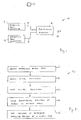
- Fig 1 schematically illustrates a satellite positioning system 10.
- the system 10 is capable of positioning one or more satellites 2.
- a satellite is an object that orbits a much greater mass such that the centre of the orbit can be approximated to the centre of the greater mass.
- Satellites may be earth satellites that orbit the earth.
- Earth satellites may be functional man-made satellites that orbit the Earth such as satellites in a Global Navigation Satellite System (GNSS).
- GNSS Global Navigation Satellite System
- the satellite 2 is a space satellite high above the Earth.
- the system 10 comprises: an empirical data generator 12; an ephemeris data generator 13; and a positioning apparatus 14. One or more of the components is located on the Earth.
- Ephemeris data generator 13 provides ephemeris (orbit) data 15 to the positioning apparatus 14.
- Ephemeris data 15 is information about the position and velocity at a particular time of one or more satellites. The same or different particular times may be used for different satellites.
- the empirical data generator 12 provides empirical based data 16 to the positioning apparatus 14.
- the empirically based data 16 accounts for the distribution of the mass of the Earth.
- the positioning apparatus 14 uses the ephemeris data 15 and the empirically based data to determine the position 17 of the satellite 2.
- the positioning apparatus 14 may output the satellite position 17.
- the positioning apparatus 14 is part of a mobile terminal. In other implementations the positioning apparatus 14 is not part of a mobile terminal but communicates the satellite position 17 to a mobile terminal.
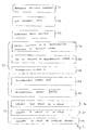
- One example of how the positioning apparatus 14 can determine the satellite position 17 is illustrated in the method 20 of Fig 2 .
- the empirically based data 16 is obtained.
- the empirically based data takes account of the gravitational potential produced by the Earth's distributed mass.
- initial conditions for the satellite are determined from the ephemeris data 15.
- the initial conditions include ⁇ int the vector velocity of the satellite at time t 0 and r int the vector position of the satellite at time t int .
- the initial conditions are mapped using defined mappings from one variable space [r, t] to another variable space [U, s]. This produces initial conditions in [U, s] space.
- the differential equation of motion of the satellite expressed using geometric algebra in terms of U and s comprises a constant based on the empirically based data 16 and this differential equation is solved using perturbation theory and the mapped initial conditions.
- an algebraic solution to the differential equation of motion of the satellite is used to determine the position of the satellite at a chosen time.
- the time scale for updating the empirical based constant can be very long. It may have a period T1, where T1>N1, in different implementations N1 can have any one of the values greater than 1 day and less than 365 days.
- the time scale for updating the empirical based constant can be very long. It may have a period T2, where T2>M1, in different implementations M1 can have any one of the values greater than 4 hours and less than 365 days. M1 may, for example, be 4 days or 2 weeks.
- Equations will identify vectors using bold notation. Vectors are identified by context within the description or may be identified using an underscore or bold font.
- Kepler's equation assumes a point source for the mass. Let us assume that the component f i with the greatest influence on f deals with the effect of mass distribution, where f i which is the gravitational field created by the uneven distribution of the earth's mass. Then to the first order f can be approximated to f i .
- u ⁇ ⁇ be a unit vector in the direction of the axis of rotation.
- v ⁇ ⁇ and w ⁇ ⁇ represent unit vectors orthogonal to u ⁇ ⁇ and orthogonal to each other.
- the dashed unit vectors rotate with the body assumed to rotate with an angular velocity of ⁇ er about the axis parallel to û and passing through the center of gravity.
- J[n][p, q, r] [ û', v ⁇ ' ⁇ '] is a multipole constant (henceforth referred to as J) that can be empirically determined. It is a set of n constants for a given set of parameters [p, q, r] and a given co-ordinate system [ û', v ⁇ ', ⁇ '].
- J may be conveyed as a set of constant values, one for each n, or may be conveyed as a single constant value (the integral) with the set of constant values being determined later using M, R and n.
- Equation 9 Use the gravitational potential expressed in Equation 9 to express the perturbation field f
- the method 30 described with reference to Fig 3 determines an unknown satellite position at a particular time. It illustrates some of the blocks of Fig 2 in more detail.
- the object of block 31 is to determine the multipole constants J up to a certain order (see equations 9 and 13 and Annex pg 29/30) that takes account of the gravitational potential produced by a distributed mass.
- the method of Fig 2 can be adapted to determine the multipole constants J up to a certain order, which when used in the method of Fig 2 determines a known satellite position at a particular time.
- the multi-pole constants J to the respective order is empirically determined as it is based on accurate ephemeris data which may be in the past.
- ephemeris data defining the initial conditions of a satellite are mapped or transformed.
- the initial conditions are mapped using defined mappings from one variable space [r, t] to another variable space [U, s]. This produces initial conditions in [U, s] space.
- the initial conditions include:
- a force constant ⁇ that is used to define the gravitational force in [U, s] space is determined.
- Equation 13 is used calculate ⁇ n U ⁇ u ⁇ ⁇ v ⁇ ⁇ w ⁇ ⁇ r ⁇ Init ⁇ r ⁇ ⁇ Init
- the force constant ⁇ is dependent upon the co-ordinate system û , v ⁇ ⁇ , w ⁇ ⁇ and on the initial conditions ⁇ int , r int . It should therefore be updated whenever new ephemeris data is to be used.
- the force constant may be distributed with or at the same time as the ephemeris data 14. For each, the force constant ⁇ need only be calculated once to yield a function in terms of U given the co-ordinate system and initial conditions.
- Equation 13 the force constant ⁇ is dependent upon J and that ⁇ is also empirically based.
- the empirically based data 13 produced by the empirical data generator 12 may be either the multipole constant J or the force constant ⁇ .
- the block includes sub-blocks 34 to 38.
- the differential equation of motion of the satellite expressed using geometric algebra in terms of U and s comprises the force constant ⁇ (see Equation 14).
- This differential equation may, for example, be solved using perturbation theory and the mapped initial conditions as explained in more detail below.
- the differential equations for the different orders of perturbation are solved to a target order of perturbation. In this example, they will be solved to the second order but in other examples a different target order for solution may be chosen.
- the first order differential equation is solved to determine Uo
- the process is continued until the target order is reached and completed.
- the target order determines accuracy.
- Equation 23 The general solution U i is found by solving equations 17 to 21 using the stability condition of Equation 23 as a constraint. (see Annex pgs 60 to 83)
- Equation 27 algebraically express ⁇ 0 D 2 ⁇ U s ⁇ U ⁇ s ⁇ ⁇ ds using the algebraic expression for U[s]U[s]' from Equation 26 in Equation 27 to determine the coefficients of Equation 27.
- Block 25 an algebraic solution to the differential equation of motion of the satellite is used to determine the position of the satellite at a chosen time.
- Block 25 comprises the sub-blocks 40 to 42.
- Equation 27 is an algebraic function that relates a time variable t to a first mapped variable s. The coefficients of this equation have been determined at block 38. At block 40, this algebraic equation is used to convert a time variable value t 1- t init to a first value s 1 of the first mapped variable.
- Equation 25 is an algebraic function that relates the first mapped variable s to the second mapped variable U.
- the coefficients of this equation have been determined at block 36.
- this algebraic equation is used to convert the first value s 1 of the first mapped variable s to a second value U(s 1 ) of a second mapped variable U.
- the satellite is positioned at block 42 by converting the second value U(s 1 ) of the second mapped variable to a position value r t1 that positions the satellite.
- the position value can then be stored in a memory for future use in applications.
- the boundary conditions (Equations 19, 20, 21) may be expressed in a look-up table in terms of the variables a, b, ⁇ o , and the initial conditions ⁇ int , r int .
- the initial conditions are defined by received ephemeris data
- the three boundary conditions are expressed in terms of variables a, b, ⁇ o in a look-up table.
- the three equations in three unknowns can be solved using standard processes (Annex pg 83) to provide a, b, ⁇ o ,
- pre-processing it is therefore possible to perform a large amount of pre-processing to obtain geometric algebraic look-up tables, which can be simply used to calculate the position. It will be appreciated that the exact extent and nature of the pre-processing may vary from implementation to implementation.
- the blocks 31, 32, 33, 24, 25 may be carried out in different locations in different apparatus.
- block 31 may, for example, be advantageous to have block 31 performed where there is access to accurate satellite positioning information. This may also be where the ephemeris data 15 is generated.
- the block 32 (mapping ephemeris data) may, for example, occur before or after distribution of ephemeris data 15.
- the block 33 may, for example, occur before distribution of the ephemeris data 15 and, for example be distributed with the ephemeris data 15.
- the block 33 may, for example, occur after receiving distributed ephemeris data 15.
- the block 24 may, for example, occur before distribution of the ephemeris data 15 and/or force constant and the coefficients may be distributed with the ephemeris data and/or force constant.
- the block 24 may, for example, occur after receiving distributed ephemeris data and after receiving or generating the force constant.
- the block 25 may, for example, occur before distribution of the ephemeris data and, for example, be distributed with the ephemeris data.
- the block 33 may, for example, occur after receiving or determining the coefficients of the algebraic expressions.
- a mobile terminal may perform blocks 31, 32, 33, 24 and 25. In another implementation a mobile terminal may perform only blocks 32, 33, 24 and 25. In another implementation a mobile terminal may perform only blocks 33, 24 and 25. In another implementation a mobile terminal may perform only blocks 24 and 25. In another implementation a mobile terminal may perform only block 25.
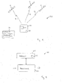
- Fig 4 schematically illustrates a Global Navigation Satellite System (GNSS) 50.
- GNSS Global Navigation Satellite System
- the system 50 comprises: a plurality of GNSS communication satellites 2 for transmitting positioning signals 51 and one or more mobile receiver terminals 52.
- a mobile receiver terminal 52 receives the positioning signals from at least some of the satellites and at least partially processes the positioning signals to determine the distance of each satellite from the mobile receiver terminal 52.
- the mobile receiver terminal 52 determines the position 53 of the mobile receiver terminal 52 by using the determined distance values for each satellite and obtained accurate positions for each satellite.
- the mobile receiver terminal 52 use the satellites positions and their distances to determine the position 53 of the mobile receiver terminal 52.
- the position 53 may be stored in a memory of the mobile receiver terminal 52.
- This system 50 may advantageously use or include the satellite positioning system 10 to provide long-term accurate satellite positions.
- the GNSS system 50 includes a system controller 54 that comprises the empirical data generator 12 and the ephemeris data generator 13.
- the empirical data generator 12 and the ephemeris data generator 13 may be housed separately using the system controller 52 or elsewhere.
- the empirical data generator 12 determines and distributes the multipole constant J and the force constant ⁇ .
- the empirical data generator 12 performs blocks 31, 32 and 33 of Fig 3 .
- the empirical data generator 12 determines and distributes only the multipole constant J and the force constant ⁇ is determined elsewhere. It may, for example, be determined in the positioning apparatus 14.
- the positioning apparatus 14 is integrated within the mobile terminal 52.
- the positioning apparatus performs blocks 24 and 25 to determine and store satellite positions 17.
- the satellite positions are used to determine and store the position 53 of the mobile receiver terminal.
- the positioning apparatus 14 may be located outside the terminal and may provide the satellite positions 17 to the mobile receiver terminal 52.
- the mobile receiver terminal 52 need not be a dedicated GNSS terminal.
- the terminal may, for example, have functionality for other uses. It may, for example, also operate as a personal digital assistant and/or a cellular phone and/or a personal music player and/or a personal video player and/or a personal computer etc.
- the position apparatus 14 can determine the position 17 of a satellite without needing to acquire current ephemeris data. This allows positioning services to be available immediately when the terminal 52 is started.
- the terminal 52 has two modes of operation. It has a first positioning mode that requires the regular receipt of ephemeris data because it expires after a few hours. It has a second positioning mode, based on the method 30 of Fig 3 , which performs block 25 to determine a satellite position 17. It may be possible for the terminal 52 to start-up in the second mode to provide instantaneous positioning and then switch to the first mode when updated ephemeris data is received. It may be possible for the terminal 52 to switch from the second mode to the first mode when it is determined that the first mode is inaccurate or potentially inaccurate.
- the determination of possible inaccuracy may occur, for example, by having a validity period for ephemeris data, after which that data expires and is no longer accurate. The determination of possible inaccuracy may occur, for example, by regularly performing the first mode and the second mode in parallel and determining when the resulting positions determined using the two modes are significantly different.
- the first mode and the second mode are performed in parallel and differences in results are used to correct for clock drift.
- Fig 5 schematically illustrates a controller 60 suitable for performing one or more of the blocks illustrated in the Figs 2 and/or 3.
- a controller of this type may be used as the empirical data generator 12 and/or the ephemeris data generator 13 and/or the positioning apparatus 14.
- the controller 60 may be implemented using instructions that enable hardware functionality, for example, by using executable computer program instructions in a general-purpose or special-purpose processor that may be stored on a computer readable storage medium (disk, memory etc) to be executed by a processor.
- a general-purpose or special-purpose processor may be stored on a computer readable storage medium (disk, memory etc) to be executed by a processor.
- the processor 62 is configured to read from and write to the memory 64.
- the processor 62 may also comprise an output interface via which data and/or commands are output by the processor 62 and an input interface via which data and/or commands are input to the processor 62.
- the memory 64 stores a computer program 66 comprising computer program instructions that control the operation of a host apparatus when loaded into the processor 62.
- the computer program instructions 66 provide the logic and routines that enables the apparatus to perform the methods illustrated in Figs 2 & 3 .
- the processor 62 by reading the memory 64 is able to load and execute the computer program 66.
- the computer program may arrive at the apparatus via any suitable delivery mechanism.
- the delivery mechanism may be, for example, a computer-readable storage medium, a computer program product, a memory device, a record medium such as a CD-ROM or DVD, an article of manufacture that tangibly embodies the computer program.
- the delivery mechanism may be a signal configured to reliably transfer the computer program 53.
- the apparatus may propagate or transmit the computer program as a computer data signal.
- memory 52 is illustrated as a single component it may be implemented as one or more separate components some or all of which may be integrated/removable and/or may provide permanent/semi-permanent/ dynamic/caclied storage.
- references to 'computer-readable storage medium', 'computer program product', 'tangibly embodied computer program' etc. or a 'controller', 'computer', 'processor' etc. should be understood to encompass not only computers having different architectures such as single /multi- processor architectures and sequential (Von Neumann)/parallel architectures but also specialized circuits such as field-programmable gate arrays (FPGA), application specific circuits (ASIC), signal processing devices and other devices.
- References to computer program, instructions, code etc. should be understood to encompass software for a programmable processor or firmware such as, for example, the programmable content of a hardware device whether instructions for a processor, or configuration settings for a fixed-function device, gate array or programmable logic device etc.
- determining the position of a satellite has many uses. It may be used to position GNSS satellites. It may be used to position and track other satellites such as space debris, which may be used to produce collision warnings. It may be used to position a satellite even after the ephemeris data has 'expired' and new ephemeris data is not available. It may be used for low power measuring of movement of a positioning apparatus 14. this may be useful when measuring landslip, structural failure, tectonic plate movement etc.
- Figs 2 and 3 may represent steps in a method and/or sections of code in the computer program.
- the illustration of a particular order to the blocks does not necessarily imply that there is a required or preferred order for the blocks and the order and arrangement of the block may be varied. Furthermore, it may be possible for some steps to be omitted.
- Module refers to a unit or apparatus that excludes certain parts/components that would be added by an end manufacturer or a user.
- the Kepler problem has been studied for a long time.
- This equation is used to calculate the orbit of a satellite orbiting round the earth in the presence of perturbing forces f.
- the solution to the equation can be obtained numerically and as the equation is non-linear the accuracy of the solution decreases the further away the point is from the initial condition.
- the transformed equation is the equation of motion of a one-dimentional harmonic oscillator.
- This equation does not have any singularities, and is also linear and is thus a good basis for performing long term analytic orbit calculations.
- Levi-Civita regularised a 2 dimensional Kepler problem, to an equivalent two dimensional harmonic oscillator. Attempts to regularise a three dimentional Kepler problem failed until 1964, when Kustaanheimo and Stiefel showed how to transform the three dimentional Kepler problem to a harmonic oscillitor in 4 dimentional space.
- the harmonic oscillator of any dimension has good analytical properties, so that make using perturbation theory, one can solve the equation of motion when there are perturbating forces present.
- Hestenes (Ref 1) showed how to solve the Kepler problem using geometric algebra, while Jan Vibrik (Ref 6) showed how to use quaternions to regularise the Kepler problem.
- Bartsch(Ref 7) gives references to Euler, Levi-Civita and Kustaanheimo and Stiefel attempts. Bartsch's paper shows how to use geometric algebra to derive a Lagrangian and Hamiltonion of the Kustaanheimo-Stiefel dynamics in arbitary static electromagnetic fields. These ideas have applications in atomic physics.
- a formula for the earth's potential V, that is represented by a spherical harmonic multipole expansion can be found in Ref 3 and refered to as the earth model.
- Quaternions are a subalgebra of geometric algebra and it would be useful to describe the regularising method using geometric algebra.
- the solution to Kepler's equation in geometric algebra is developed in Ref 1, but only for axially symmetric bodies.
- the advantage of evaluating the RHS in geometric algebra is that the level of perturbation approximation needed can be decided depending on the length of time that has elapsed between the last known position of the satellite and the time for which the position is required.
- the perturbation level can be precalculated beforehand, and the different solutions stored.
- r and r' may not commute. r r' may not be equal to r' r.
- P n are usually known as Legendre polynomials.We need to prove that all the terms are accounted for. For any i and k, the term - 1 2 ⁇ C i * iC k * - 2 ⁇ r . r ⁇ i - k r ⁇ 2 ⁇ k ) r 2 ⁇ i
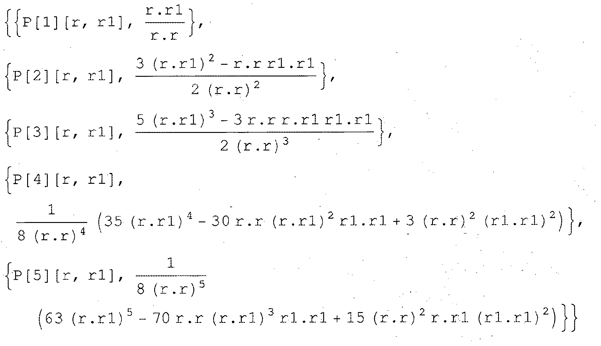
- the Legendre polynomials are generated by the following code.
- the first five Legendre polynomials are generated by the following code
- the origin be the center of gravity of the body.
- the dashed unit vectors rotate with the body assumed to rotate with an angular velocity of ⁇ er about the axis parallel to û and passing through the center of gravity.
- G ⁇ 1 r ⁇ P 2 r ⁇ r ⁇ ⁇ dm ⁇ ⁇ r ⁇ G ⁇ 1 r ( 1 2 ⁇ r 4 ⁇ 3 ⁇ r . u ⁇ 2 ⁇ u ⁇ ⁇ 2 + 3 ⁇ r 2 ⁇ w ⁇ ⁇ 2 - 3 ⁇ r . u ⁇ 2 ⁇ w ⁇ ⁇ 2 - r 2 ⁇ u ⁇ ⁇ 2 - 2 ⁇ r 2 ⁇ w ⁇ ⁇ 2 dm ⁇ ⁇ r ⁇
- G ⁇ 1 r ⁇ P 2 r ⁇ r ⁇ ⁇ dm ⁇ ⁇ r ⁇ G ⁇ 1 r ( 1 2 ⁇ r 4 ⁇ 3 ⁇ r . u ⁇ 2 ⁇ u ⁇ ⁇ 2 + r 2 ⁇ w ⁇ ⁇ 2 - 3 ⁇ r . u ⁇ 2 ⁇ w ⁇ ⁇ 2 - r 2 ⁇ u ⁇ ⁇ 2 ⁇ dm ⁇ ⁇ r ⁇
- J 2 Given axial symmetry, we can express J 2 as above, where J 2 has the usual definitions.
- the quaternion implementation of the solution to Kepler's equation for predicting orbits is transformed into finding the root by numerical means of an equation, as opposed to numerically solving a non linear differential equation.
- the quaternion implementation has therefore superior numerical accuracy.
- Quaternions are a subalgebra of geometric algebra and it would be useful to describe the regularising method using geometric algebra.
- the solution to Kepler's equation in geometric algebra is developed in Ref 1, but only for axially symmetric bodies.
- J[n][p, q, r] [ û ', v ⁇ ', ⁇ '] are functions of the unit vectors û' , v ⁇ ' , ⁇ ' , and for a particular coordinate system for each p,q, and r , the value of J[n] [p, q, r] [ û ', v ⁇ ', ⁇ '] can be determined empirically for the earth, given the trajectories of orbiting satellites.
- J[1] [0, 0, 1] [u, v, ⁇ ],J[1] [0, 1, 0] [û, v ⁇ , ⁇ ] and J [1] [1, 0, 0] [û, v ⁇ , ⁇ ] are zero.
- the angular momentum for unit mass is defined as L ⁇ r ⁇ r •
- ⁇ n [U, û , v ⁇ , ⁇ , r ⁇ Init , ⁇ Init ] also depends on the constants multipole constants, J [n] [p, q, r] [ û , v ⁇ , ⁇ ].
- J[n] [p, q, r] [ û , v ⁇ , ⁇ ] is a constant.
- ⁇ n [U, û , v ⁇ , ⁇ , r ⁇ Init , ⁇ Init need only be calculated once, to yield a function in terms of U, given the initial position r Init , and initial velocity ⁇ Init , and the unit vectors û, v ⁇ , ⁇ , as ⁇ n [U, û , v ⁇ , ⁇ , r ⁇ Init , ⁇ Init ] then just depends on U, the rest of the inputs being constant.
- the above equation is an example of a weakly non-linear equation to which one may apply perturbation techniques e.g Lindstedt-Poincare (Ref 4) to generate analytic solutions correct to a given order.
- Vrbik (Ref 8) has produced perturbed solutions to orbits using quaternion.
- ⁇ Sin , and ⁇ cos are the number of terms to use for the desired accuracy and j is complex square root of -1.
- the number of terms to use depends on the orbit of the satellite. When the encentricity of the orbit is small, then only a few terms need be used. For satellite orbits which are nearly circular, then only as few as 4 terms may be sufficient. Also, if it is possible to select the initial position, then select the position that is approximately the square root of the product of the nearest and furtherst distances.
- ⁇ n U ⁇ u ⁇ ⁇ v ⁇ ⁇ w ⁇ ⁇ r ⁇ Init ⁇ r ⁇ ⁇ Init can be expressed as a sum of therms that are products of terms that can be expresses as exponentials.
- the right hand side of the second equation can be expressed as a sum of exponentials
- ⁇ [k] is a non-linear equation, for k>1, and entirely in terms of the initial conditions once we have solved for a,b, and ⁇ 0 .
- One of the methods of solving it would be to get an estimate of s 1 , using, ⁇ [0], the zero order perturbation equation, then using the solution of ⁇ [0] as initial input for Newton-Raphson method for solving ⁇ [1], and so on until one arrives at the solution for the appropriate equation to be solved.
- t 0 we know the position of the position of the satellite and its velocity.
- the first limit can be expressed as two limits, because interchanging the order of the limits yields the same limit point.
- ⁇ k 1 n ⁇ k ( r n ⁇ Limit ⁇ k ⁇ 0 1 ⁇ k ⁇ 1 + 2 ⁇ k r . ⁇ k + ⁇ k 2 ⁇ ⁇ k 2 r 2 n 2 - 1 )
- r n ⁇ r 1 r n ⁇ r ⁇ . u m
- ⁇ r r . u m r m m ⁇ r . u m - 1 r m ⁇ u - m ⁇ r . u m r m + 2 r
Landscapes
- Engineering & Computer Science (AREA)
- Radar, Positioning & Navigation (AREA)
- Remote Sensing (AREA)
- Power Engineering (AREA)
- Computer Networks & Wireless Communication (AREA)
- Physics & Mathematics (AREA)
- General Physics & Mathematics (AREA)
- Position Fixing By Use Of Radio Waves (AREA)
Abstract
Description
- Embodiments of the present invention relate to positioning satellites. In particular, they relate to positioning satellites using solutions derived by geometric algebraic methods to equations of motion.
- Typically the differential equation of motion for a satellite orbiting the earth is solved numerically to determine the future positions of the satellites. This means that the determined future positions are only accurate with a limited time window typically a few hours.
- According to various, but not necessarily all, embodiments of the invention there is provided embodiments as described in the appended claims.
- Some embodiments of the invention by using geometric algebraic solutions enable long term accurate positioning without the need for current ephemeris data. The inherent accuracy of the geometric algebraic solutions (compared to numeric solutions) enables the positioning of an apparatus without having to download current ephemeris data.
- Current positioning solutions (which use numeric solutions) require updated ephemeris data every 2 to 4 hours because the accuracy of the numeric solution decreases with time. The inventive solution proposed here is better able to accurately determine the future positions of satellites because it provides a geometric algebraic solution of designed (predetermined) accuracy. It will be able to work accurately using ephemeris data for a chosen duration into the future that may be days, weeks or even months.
- This will enable the positioning of an apparatus when it is switched on without first having to download the current ephemeris data. The location of the apparatus will therefore be determined more quickly.
- The use of pre-calculated algebraic look-up tables may be used to provide fast positioning.
- The (real world) position of an apparatus is a technical feature of the apparatus. Thus the positioning or locating of an apparatus provides technical effect.
- In the example given below, the perturbation order determines the accuracy of the positioning calculation into the future. For longer term accuracy, more orders are required. As the perturbation calculation starts at the lowest order and the solution to that order is used to determine the solution to the next highest order, the perturbation calculation may be stopped at the required order of accuracy. A look up table may indicate the order required for a particular duration into the future. Thus the perturbation order may be a dynamic variable of the calculation.
- The number of terms in the expansion (Annex pg 68) also affects the fundamental accuracy of the calculations. Accuracy may be improved by including more terms. Thus the number of terms may be a dynamic variable of the calculation.
- It will be appreciated that real world positioning has many applications. It may, for example, be used in navigation apparatus, in emergency apparatus, in apparatus that provide location dependent services, etc.
- Embodiments of the invention may result in a satellite positioning system transmitting less (or no) ephemeris data. This may result in fewer satellite tracking stations. This may enable the use of longer pseudo codes in satellite transmissions which would result in greater sensitivity of receivers. This could free up bandwidth in the satellite transmissions which could be used for other purposes.
- Embodiments of the invention enables fast positioning by occasional-use positioning apparatus, that have pre-stored or 'old' ephemeris data.
- For a better understanding of various examples of embodiments of the present invention reference will now be made by way of example only to the accompanying drawings in which:
-
Fig 1 schematically illustrates a satellite positioning system; -
Fig 2 schematically illustrates a method for determining a satellite position; -
Fig 3 schematically illustrates, in detail, for determining an unknown satellite position at a particular time; -
Fig 4 schematically illustrates a Global Navigation Satellite System (GNSS); and -
Fig 5 schematically illustrates a controller. -
Fig 1 schematically illustrates asatellite positioning system 10. Thesystem 10 is capable of positioning one ormore satellites 2. A satellite is an object that orbits a much greater mass such that the centre of the orbit can be approximated to the centre of the greater mass. Satellites may be earth satellites that orbit the earth. Earth satellites may be functional man-made satellites that orbit the Earth such as satellites in a Global Navigation Satellite System (GNSS). InFig 1 , thesatellite 2 is a space satellite high above the Earth. - The
system 10 comprises: an empirical data generator 12; anephemeris data generator 13; and apositioning apparatus 14. One or more of the components is located on the Earth. - The
ephemeris data generator 13 provides ephemeris (orbit) data 15 to thepositioning apparatus 14. Ephemeris data 15 is information about the position and velocity at a particular time of one or more satellites. The same or different particular times may be used for different satellites. - The empirical data generator 12 provides empirical based
data 16 to thepositioning apparatus 14. The empirically baseddata 16 accounts for the distribution of the mass of the Earth. - The
positioning apparatus 14 uses the ephemeris data 15 and the empirically based data to determine theposition 17 of thesatellite 2. Thepositioning apparatus 14 may output thesatellite position 17. - Although a
single satellite 2 is illustrated, it should be appreciated that a plurality of satellites may be positioned by thepositioning apparatus 14. - In some implementations the
positioning apparatus 14 is part of a mobile terminal. In other implementations thepositioning apparatus 14 is not part of a mobile terminal but communicates thesatellite position 17 to a mobile terminal. - One example of how the
positioning apparatus 14 can determine thesatellite position 17 is illustrated in themethod 20 ofFig 2 . - At block 21, the empirically based
data 16 is obtained. The empirically based data takes account of the gravitational potential produced by the Earth's distributed mass. - At block 22, initial conditions for the satellite are determined from the ephemeris data 15. The initial conditions include ṙ int the vector velocity of the satellite at time t0 and r int the vector position of the satellite at time tint.
- At
block 23, the initial conditions are mapped using defined mappings from one variable space [r, t] to another variable space [U, s]. This produces initial conditions in [U, s] space. - At
block 24, a differential equation of motion of the satellite, expressed using geometric algebra in terms of U and s is solved. - The differential equation of motion of the satellite, expressed using geometric algebra in terms of U and s comprises a constant based on the empirically based
data 16 and this differential equation is solved using perturbation theory and the mapped initial conditions. - At
block 25, an algebraic solution to the differential equation of motion of the satellite is used to determine the position of the satellite at a chosen time. - The use of algebraic as opposed to numerical solutions gives a solution that has a very long, theoretically infinite, validity period. The accuracy is selectable and depends upon the order of the perturbation solutions.
- The time scale for updating the empirical based constant can be very long. It may have a period T1, where T1>N1, in different implementations N1 can have any one of the values greater than 1 day and less than 365 days.
- The time scale for updating the empirical based constant can be very long. It may have a period T2, where T2>M1, in different implementations M1 can have any one of the values greater than 4 hours and less than 365 days. M1 may, for example, be 4 days or 2 weeks.
- This section outlines the mathematics used in one method of positioning a satellite. A full and detailed explanation of the mathematics is included as an Annex to the description.
- In this section, the Equations will identify vectors using bold notation. Vectors are identified by context within the description or may be identified using an underscore or bold font.
- In this section the Kepler equation is re-expressed using the variables r and U giving a new equation of motion.
- The Kepler Equation for motion in a gravitational field is:

- r is the distance of the satellite from the origin
- f is a force that accounts for the distribution of the attracting mass
- Make the following definitions:


- σ1 is a unit vector (later referred to as r̂ int )
- U is a geometric algebraic multivector (bivector)
- Re-expressing Kepler's Equation of motion (equation 4) using geometric algebra in terms of U and f as defined in
Equations 2 and 3 gives:
E is theKepler energy 
- The perturbation force f may be expressed as a vector sum of a plurality of forces fi e.g. f = Σfi.
- Kepler's equation assumes a point source for the mass. Let us assume that the component fi with the greatest influence on f deals with the effect of mass distribution, where fi which is the gravitational field created by the uneven distribution of the earth's mass. Then to the first order f can be approximated to fi.
- In this section the force f will be expressed using geometric algebra as a multi-pole function (when no axial symmetry is assumed) in terms of U.
- The stages to this are:
- a) Initially the multi-pole function is initially expressed in terms of P,
- b) then in terms of an arbitrary coordinate system without assuming axial symmetry,
- c) then finally expressed in terms of U.
- Gravitational potential is expressed as:

- A multipole expansion is performed using geometric algebra as:


where Pn is the Legendre polynomial of order n and Cn are the coefficients of a Taylor series (standard binomial coefficients). There is no assumption of spherical symmetry. - The gravitational potential can then be expressed using the multipole expansion
(Equation 1)
(Annex pg 12)
ϕ is the gravitational potential created by the uneven distribution of the earth's mass expressed as location dependent values. - We now define an arbitrary orthogonal rectilinear co-ordinate system
- Let


- We can express r' as


- The dashed unit vectors rotate with the body assumed to rotate with an angular velocity of ωer about the axis parallel to û and passing through the center of gravity.

- Re expressing
Equation 7 using Equation 8


- Use the gravitational potential expressed in Equation 9 to express the perturbation field f

- This can be alternatively expressed as

- Re-express the equation of motion (Equation 5) using Equation 11


- Given the initial position vector r Init and velocity vector r̂ Init of the orbiting body, we can specify the bivector component of U to be proportional to


(Annex pg 40)
Using

- Define


- The division by rint maintains precision.
- Define a new constant

- This is a constant for at a particular initial condition defined in the co-ordinate system u, v, w. It is empirically based as it depends upon J. Although described as a constant, it should be appreciated that Γ is a set of constant values, one for each n. Re-express Equation 12 using
Equation 13
f is thus expressed using geometric algebra in terms of U. It is a multipole function that includes an empirically based constant Γ. - The Equation is then solved using perturbation theory,
- Define


- And let

- Where

- Defining

- The perturbed equation of motion is given by


- A solution of the following form is assumed:

where, the following stability condition holds:


- It should also be noted that from Equation 2

also fromEquation 2
- The method 30 described with reference to
Fig 3 determines an unknown satellite position at a particular time. It illustrates some of the blocks ofFig 2 in more detail. - The object of
block 31 is to determine the multipole constants J up to a certain order (seeequations 9 and 13 and Annex pg 29/30) that takes account of the gravitational potential produced by a distributed mass. - The method of
Fig 2 can be adapted to determine the multipole constants J up to a certain order, which when used in the method ofFig 2 determines a known satellite position at a particular time. - By using additional ephemeris data that accurately identifies satellite positions at different times, it is possible to generate a series of equations in which the unknown is the multipole constants J to the desired order. Optimisation techniques may then be used to determine the common unknown multipole constants.
- For example, if the positions ri of a satellite are known accurately at different times ti, then there will be values si associated with ti. Substituting ri and ti into the
Equations 3 and 25 results in two equations with unknowns J and the respective si. - These equations may be solved using least mean square techniques. Many different accurate positions for the same satellite ri at known times ti may be used to increase accuracy. The method may also be repeated with additional satellites to increase accuracy.
- The multi-pole constants J to the respective order is empirically determined as it is based on accurate ephemeris data which may be in the past.
- At
block 32, ephemeris data defining the initial conditions of a satellite are mapped or transformed. The initial conditions are mapped using defined mappings from one variable space [r, t] to another variable space [U, s]. This produces initial conditions in [U, s] space. - The initial conditions include:
- ṙ int
- is the vector velocity of the satellite at time tint
- r int
- is the vector displacement of the satellite at time tinit
- The equations 28 and 29 are used to perform the mapping.
- At block 33, a force constant Γ that is used to define the gravitational force in [U, s] space is determined.
-
Equation 13 is used calculate

- The force constant Γ is dependent upon the co-ordinate system û,

ephemeris data 14. For each, the force constant Γ need only be calculated once to yield a function in terms of U given the co-ordinate system and initial conditions. - It will be appreciated from
Equation 13 that the force constant Γ is dependent upon J and that Γ is also empirically based. - The empirically based
data 13 produced by the empirical data generator 12 may be either the multipole constant J or the force constant Γ. - At
block 24, a differential equation of motion of the satellite, expressed using geometric algebra in terms of U and s is solved. The block includes sub-blocks 34 to 38. - The differential equation of motion of the satellite, expressed using geometric algebra in terms of U and s comprises the force constant Γ (see Equation 14). This differential equation may, for example, be solved using perturbation theory and the mapped initial conditions as explained in more detail below.
- At block 34, the differential equations for the different orders of perturbation are solved to a target order of perturbation. In this example, they will be solved to the second order but in other examples a different target order for solution may be chosen.
- The first order differential equation is solved to determine Uo
- The next order differential equation is simplified using the first order differential equation and its determined solution Uo. The equation is then solved to determine U1
- In general, the rth order differential equation is simplified using the (r-1)th order differential equation and its determined solutions Ui. The equation is then solved to determine Ur
- The process is continued until the target order is reached and completed. The target order determines accuracy.
- The general solution Ui is found by solving
equations 17 to 21 using the stability condition ofEquation 23 as a constraint. (see Annex pgs 60 to 83) - At
block 35, express the obtained solutions Ui for each perturbation order using thealgebraic equation 24 and determine the coefficients of Equation 22.
- At block 36, algebraically express U using the algebraic expression for Ui from
Equation 24 inEquation 25 and determine the coefficients ofEquation 25.
- At block 37, algebraically express U[s] U[s]+ using the algebraic expression for U from
Equation 25 in Equation 26 and determine the coefficients of Equation 26.
- At block 38, algebraically express


- At
block 25, an algebraic solution to the differential equation of motion of the satellite is used to determine the position of the satellite at a chosen time.Block 25 comprises the sub-blocks 40 to 42. - Equation 27 is an algebraic function that relates a time variable t to a first mapped variable s. The coefficients of this equation have been determined at block 38. At block 40, this algebraic equation is used to convert a time variable value t1-tinit to a first value s1 of the first mapped variable.
-
Equation 25 is an algebraic function that relates the first mapped variable s to the second mapped variable U. The coefficients of this equation have been determined at block 36. Atblock 41, this algebraic equation is used to convert the first value s1 of the first mapped variable s to a second value U(s1) of a second mapped variable U. - The satellite is positioned at block 42 by converting the second value U(s1) of the second mapped variable to a position value rt1 that positions the satellite. The mapping between [r, t] and [U, s] (Equation 2) is used to determine rt1

- The position value can then be stored in a memory for future use in applications.
- This approach provides an algebraic solution the accuracy of which is dependent upon the target order of perturbation elected and used. The accuracy is not time dependent. Assuming there is no change to the perturbation force the validity period is theoretically infinite at an accuracy determined by the 'depth' of algebraic solution (i.e. the target order of perturbation used). Consequently there is no requirement to repeatedly send or receive ephemeris data and ephemeris data may be pulled by the positioning apparatus rather than pushed to the positioning apparatus.
- It should be appreciated that the various blocks in
Fig 2 and3 need not be performed by a single apparatus. - For example, the boundary conditions (
Equations 19, 20, 21) may be expressed in a look-up table in terms of the variables a, b, ωo, and the initial conditions ṙ int, r int. When the initial conditions are defined by received ephemeris data the three boundary conditions are expressed in terms of variables a, b, ωo in a look-up table. The three equations in three unknowns can be solved using standard processes (Annex pg 83) to provide a, b, ωo, - The equation below may be expressed in a look-up table as a function of a, b, wo, t, and s:

- Once a, b, ωo have been determined for a set of initial conditions ṙ int, r int, the value s at any arbitrary future time t can be simply determined.
- The equation below may be expressed in a look-up table as a function of a, b, ωo, and s (Annex pg 82):

- The position can then be simply calculated

- It is therefore possible to perform a large amount of pre-processing to obtain geometric algebraic look-up tables, which can be simply used to calculate the position. It will be appreciated that the exact extent and nature of the pre-processing may vary from implementation to implementation.
- If more than on constellation may be used for positioning (e.g. GPS, Galileo, Clonass etc), then it may be advantage to nest the look-up tables such that those relating to a particular constellation are stored logically together. This improves access speed. Referring to
Fig 4 theblocks - It may, for example, be advantageous to have
block 31 performed where there is access to accurate satellite positioning information. This may also be where the ephemeris data 15 is generated. - The block 32 (mapping ephemeris data) may, for example, occur before or after distribution of ephemeris data 15.
- The block 33 (determining force constant) may, for example, occur before distribution of the ephemeris data 15 and, for example be distributed with the ephemeris data 15. Alternatively, the block 33 (determining force constant) may, for example, occur after receiving distributed ephemeris data 15.
- The block 24 (determining the coefficients of the algebraic expressions) may, for example, occur before distribution of the ephemeris data 15 and/or force constant and the coefficients may be distributed with the ephemeris data and/or force constant. Alternatively, the block 24 (determining the coefficients of algebraic expressions) may, for example, occur after receiving distributed ephemeris data and after receiving or generating the force constant.
- The block 25 (determining position) may, for example, occur before distribution of the ephemeris data and, for example, be distributed with the ephemeris data. Alternatively, the block 33 (determining force constant) may, for example, occur after receiving or determining the coefficients of the algebraic expressions.
- In one implementation a mobile terminal may perform
blocks -
Fig 4 schematically illustrates a Global Navigation Satellite System (GNSS) 50. - The
system 50 comprises: a plurality ofGNSS communication satellites 2 for transmitting positioning signals 51 and one or moremobile receiver terminals 52. - A
mobile receiver terminal 52 receives the positioning signals from at least some of the satellites and at least partially processes the positioning signals to determine the distance of each satellite from themobile receiver terminal 52. - The
mobile receiver terminal 52 determines theposition 53 of themobile receiver terminal 52 by using the determined distance values for each satellite and obtained accurate positions for each satellite. Themobile receiver terminal 52 use the satellites positions and their distances to determine theposition 53 of themobile receiver terminal 52. Theposition 53 may be stored in a memory of themobile receiver terminal 52. - Typically four or more satellites need to be in sight and the satellite positions need to be accurate.
- This
system 50 may advantageously use or include thesatellite positioning system 10 to provide long-term accurate satellite positions. - For example, in this example the
GNSS system 50 includes asystem controller 54 that comprises the empirical data generator 12 and theephemeris data generator 13. In other implementations the empirical data generator 12 and theephemeris data generator 13 may be housed separately using thesystem controller 52 or elsewhere. - In the illustrated example, the empirical data generator 12 determines and distributes the multipole constant J and the force constant Γ. The empirical data generator 12 performs
blocks Fig 3 . However, in other implementations the empirical data generator 12 determines and distributes only the multipole constant J and the force constant Γ is determined elsewhere. It may, for example, be determined in thepositioning apparatus 14. - In this illustrated example, the
positioning apparatus 14 is integrated within themobile terminal 52. The positioning apparatus performsblocks position 53 of the mobile receiver terminal. In other implementations thepositioning apparatus 14 may be located outside the terminal and may provide the satellite positions 17 to themobile receiver terminal 52. - The
mobile receiver terminal 52 need not be a dedicated GNSS terminal. The terminal may, for example, have functionality for other uses. It may, for example, also operate as a personal digital assistant and/or a cellular phone and/or a personal music player and/or a personal video player and/or a personal computer etc. - There is no significant time delay in positioning the terminal 52 immediately after starting-up the terminal 52. The
position apparatus 14 can determine theposition 17 of a satellite without needing to acquire current ephemeris data. This allows positioning services to be available immediately when the terminal 52 is started. - In one embodiment, the terminal 52 has two modes of operation. It has a first positioning mode that requires the regular receipt of ephemeris data because it expires after a few hours. It has a second positioning mode, based on the method 30 of
Fig 3 , which performsblock 25 to determine asatellite position 17. It may be possible for the terminal 52 to start-up in the second mode to provide instantaneous positioning and then switch to the first mode when updated ephemeris data is received. It may be possible for the terminal 52 to switch from the second mode to the first mode when it is determined that the first mode is inaccurate or potentially inaccurate. The determination of possible inaccuracy may occur, for example, by having a validity period for ephemeris data, after which that data expires and is no longer accurate. The determination of possible inaccuracy may occur, for example, by regularly performing the first mode and the second mode in parallel and determining when the resulting positions determined using the two modes are significantly different. - In another embodiment, the first mode and the second mode are performed in parallel and differences in results are used to correct for clock drift.
-
Fig 5 schematically illustrates acontroller 60 suitable for performing one or more of the blocks illustrated in theFigs 2 and/or 3. A controller of this type may be used as the empirical data generator 12 and/or theephemeris data generator 13 and/or thepositioning apparatus 14. - The
controller 60 may be implemented using instructions that enable hardware functionality, for example, by using executable computer program instructions in a general-purpose or special-purpose processor that may be stored on a computer readable storage medium (disk, memory etc) to be executed by a processor. - The
processor 62 is configured to read from and write to thememory 64. Theprocessor 62 may also comprise an output interface via which data and/or commands are output by theprocessor 62 and an input interface via which data and/or commands are input to theprocessor 62. - The
memory 64 stores a computer program 66 comprising computer program instructions that control the operation of a host apparatus when loaded into theprocessor 62. The computer program instructions 66 provide the logic and routines that enables the apparatus to perform the methods illustrated inFigs 2 &3 . Theprocessor 62 by reading thememory 64 is able to load and execute the computer program 66. - The computer program may arrive at the apparatus via any suitable delivery mechanism. The delivery mechanism may be, for example, a computer-readable storage medium, a computer program product, a memory device, a record medium such as a CD-ROM or DVD, an article of manufacture that tangibly embodies the computer program. The delivery mechanism may be a signal configured to reliably transfer the
computer program 53. The apparatus may propagate or transmit the computer program as a computer data signal. - Although the
memory 52 is illustrated as a single component it may be implemented as one or more separate components some or all of which may be integrated/removable and/or may provide permanent/semi-permanent/ dynamic/caclied storage. - References to 'computer-readable storage medium', 'computer program product', 'tangibly embodied computer program' etc. or a 'controller', 'computer', 'processor' etc. should be understood to encompass not only computers having different architectures such as single /multi- processor architectures and sequential (Von Neumann)/parallel architectures but also specialized circuits such as field-programmable gate arrays (FPGA), application specific circuits (ASIC), signal processing devices and other devices. References to computer program, instructions, code etc. should be understood to encompass software for a programmable processor or firmware such as, for example, the programmable content of a hardware device whether instructions for a processor, or configuration settings for a fixed-function device, gate array or programmable logic device etc.
- It should be appreciated that determining the position of a satellite has many uses. It may be used to position GNSS satellites. It may be used to position and track other satellites such as space debris, which may be used to produce collision warnings. It may be used to position a satellite even after the ephemeris data has 'expired' and new ephemeris data is not available. It may be used for low power measuring of movement of a
positioning apparatus 14. this may be useful when measuring landslip, structural failure, tectonic plate movement etc. - Various components may have been described as connected in the preceding paragraphs. It should be appreciated that they may instead be operationally coupled and any number or combination of intervening elements can exist (including no intervening elements)
- Reference has been made to various examples in the preceding description. It should be understood that reference to an example implies that alternative, but not necessarily explicitly disclosed implementations can be used.
- The blocks illustrated in
Figs 2 and3 may represent steps in a method and/or sections of code in the computer program. The illustration of a particular order to the blocks does not necessarily imply that there is a required or preferred order for the blocks and the order and arrangement of the block may be varied. Furthermore, it may be possible for some steps to be omitted. - As used here 'apparatus' includes devices, modules, systems. Module refers to a unit or apparatus that excludes certain parts/components that would be added by an end manufacturer or a user.
- Although embodiments of the present invention have been described in the preceding paragraphs with reference to various examples, it should be appreciated that modifications to the examples given can be made without departing from the scope of the invention as claimed.
- Features described in the preceding description may be used in combinations other than the combinations explicitly described.
- Although functions have been described with reference to certain features, those functions may be performable by other features whether described or not.
- Although features have been described with reference to certain embodiments, those features may also be present in other embodiments whether described or not.
- Whilst endeavoring in the foregoing specification to draw attention to those features of the invention believed to be of particular importance it should be understood that the Applicant claims protection in respect of any patentable feature or combination of features hereinbefore referred to and/or shown in the drawings whether or not particular emphasis has been placed thereon.
- We will be using geometric algebra to perform the calculations, using the spinor formulation.
- The Kepler problem has been studied for a long time. The equation of motion

- Euler was the first person to transform the equation so that one could study the long term evolution of the quantities of interest. For the one-dimentional Kepler equation without any perturbing forces,

- Euler found a transformation, so that the equation became

- The transformed equation is the equation of motion of a one-dimentional harmonic oscillator. This equation does not have any singularities, and is also linear and is thus a good basis for performing long term analytic orbit calculations. Levi-Civita regularised a 2 dimensional Kepler problem, to an equivalent two dimensional harmonic oscillator. Attempts to regularise a three dimentional Kepler problem failed until 1964, when Kustaanheimo and Stiefel showed how to transform the three dimentional Kepler problem to a harmonic oscillitor in 4 dimentional space. The harmonic oscillator of any dimension has good analytical properties, so that make using perturbation theory, one can solve the equation of motion when there are perturbating forces present. Hestenes (Ref 1) showed how to solve the Kepler problem using geometric algebra, while Jan Vibrik (Ref 6) showed how to use quaternions to regularise the Kepler problem. Bartsch(Ref 7) gives references to Euler, Levi-Civita and Kustaanheimo and Stiefel attempts. Bartsch's paper shows how to use geometric algebra to derive a Lagrangian and Hamiltonion of the Kustaanheimo-Stiefel dynamics in arbitary static electromagnetic fields. These ideas have applications in atomic physics.
- We have derived an expression for the solution to the equation of motion of a satellite, without assuming that the earth is axially symmetric using geometric algebra, and it is this geometric algebra version that is novel. Jan Vibrik has derived a similar solution to the equation using quaternions and purterbation theory. We derive a geometric algebra equation, the right hand side of which can be evaluated first in geometric algebra (We have in Note B provided an example of a Mathematica program where we have implemented the rules of the geometric vector product.)
- A formula for the earth's potential V, that is represented by a spherical harmonic multipole expansion can be found in Ref 3 and refered to as the earth model.
- We derive, a multipole expansion, similar to the earth model, in that we do not assume axial symmetry of the body, but without needing to specify the coordinate system (such as spherical harmonic in the earth model) . This multipole expansion differs from the multipole expansion found in
reference 1. - The quaternion implementation of the solution to Kepler's equation for predicting orbits has been known to have superior numerical properties (See Ref 6). Also, this quote, "Quaternions have been found to be the ideal tool for describing and developing the theory of spatial regularization in celestial mechanics" can be found in Ref 5.
- Quaternions are a subalgebra of geometric algebra and it would be useful to describe the regularising method using geometric algebra. The solution to Kepler's equation in geometric algebra is developed in
Ref 1, but only for axially symmetric bodies. - The advantage of evaluating the RHS in geometric algebra is that the level of perturbation approximation needed can be decided depending on the length of time that has elapsed between the last known position of the satellite and the time for which the position is required. The perturbation level can be precalculated beforehand, and the different solutions stored.
- In order to calculate the perturbing force f, we need the series expansion of the expression.


- We consider the contribution to the gravitional field at point P due to the mass dm' at r' of a body that may not possess spherical symmetry.

- We use bold letters for vectors.
- | r - r' | represents the length of the vector (r - r'). But in GA, r 2 = r 2, the square of the length of vector r. Thus | r - r '|2 = ( r - r')2 . Thus we get

- Multiplying out the expression we get

- Note that the vectors r and r' may not commute. r r' may not be equal to r' r.
- But in GA, r 2 = r 2, the square of the length of vector r. Similarly, (r')2 = (r')2. Also in GA, we have for the dot product,

- Substituting these, we get

- Now the expression on the right is made up entirely of scalar terms, and we can manuplate the terms using the usual rules of real analysis since multiplication of real numbers is always commutative. Multiplication of vectors in geometric algebra is not necessarily commutative.
- As r » r' we can write this as

- Or as

- Expand as a Taylor's
series 
- where mCn are the usual binomial coefficients. Thus we get

- We can expand the power to get

- Distributing we get

- Now we consider all the terms that can be expressed as powers of
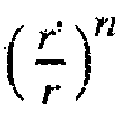


- Or using a different formula,
we can express Pn
- Pn are usually known as Legendre polynomials.We need to prove that all the terms are accounted for. For any i and k, the term

- is summed in the expression P i+k [r, r']. Thus each of the terms of the series expansion is in exactly one Legendre expression.
- The Legendre polynomials are generated by the following code.

- The first five Legendre polynomials are generated by the following code

- The results are

- Let r = r[τ] be the orbit of a particle of unit mass with the equation of motion

- Let σ1 be a fixed unit vector, U a quaternion that varies with t, such that

- There is some freedom in the choice of U. We can choose U, such that U satisfies

- The above equation is the commonly known as the subsidiary condition.

- That implies

- From the above equation, r = r r̂, and r = U † σ1 U we get

- And

- From


- Thus we get

- But by applying the grade operator to both sides

- Distributing

- Applying revision to the second term

- Thus we get

- But since


- Thus

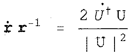
- Simplifying
- We can multiply LHS by r and the RHS by U † σ1 U

- Simplifying


- Taking the reversion of both sides of the equation, and rembering ṙ is a vector,


- We now consider what happens when we differentiate both sides with respect to t. Remember, σ1 is a constant of unit length.

- Multiplying the second term of LHS by


- Using the transformation equation r = U † σ1 U, we can simply the second term of
LHS 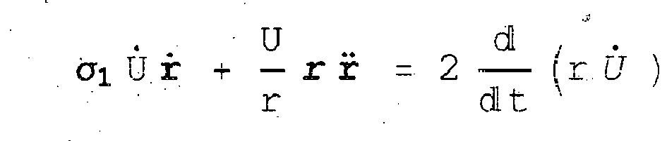
- Using the
equation 
LHS 
- Simplifying the first term of
LHS 
- Factorising the LHS of the above equation

- Define a new variable

- The RHS of the equation is

- Multiplying both sides of the equation by r

- We simplify RHS as

- Now given the equation of motion

- We get by multiplying both sides by r. (Note that we are performing a geometric product of two vectors, and so order of the multipicants does matter)

- Remembering that r and r̂ are parallel vectors, we have r r̂ = r. Thus we get for the equation of motion

- Substituting for r ṙ in

- We get

- Rearranging the RHS, using the distribution law,

- This can be expressed as


- Rearranging the equation we get the geometric algebra equation, which can be solved by perturbation theory.

- Now we calculate the perturbation forces f.

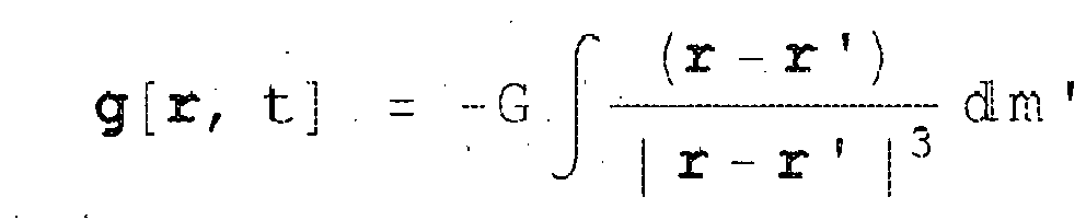
- We define the origin to be the center of gravity of the body. Then, for a continuous body, the field, g[r,t], due to the body at a point P,situated r from the origin, at time t, is defined to be
- The potential for the same body at the same point P is given by

- We have

- Thus we get

- We list the first five Legrendre Polynomials Pn [ r, r']


- We list the corresponding Legrendre Polynomials Pn [ r̂ , r̂ '], given unit vectors r̂, r̂' as input.


- Distributing the integration

- The first integral on the RHS of the expression is

- Where M is the mass of the earth
- We calculate the 1,2,3... terms of the multipole expansion of the potential function φ[r, t]. The first term in the multipole expansion is

- Substituting for P 1, we get

- Simplifying, and factoring r, and


- But the integral ∫r' dm' [r'], is zero, as we locate the origin at the center of gravity of the body.

- For n = 2

- Let û be a unit vector in the direction of the axis of rotation. Let v̂ and ŵ represent unit vectors orthogonal to û and orthogonal to each other. Then

- We can express r' as


- The dashed unit vectors rotate with the body assumed to rotate with an angular velocity of ωer about the axis parallel to û and passing through the center of gravity.
- Remember because of the orthogonality assumption of unit vectors

- Substituting for P2

- Substituting for (r')2 = (r')2

- Substituting for r'

- Expressing û', v̂', ŵ' in terms of û, v̂, and ŵ

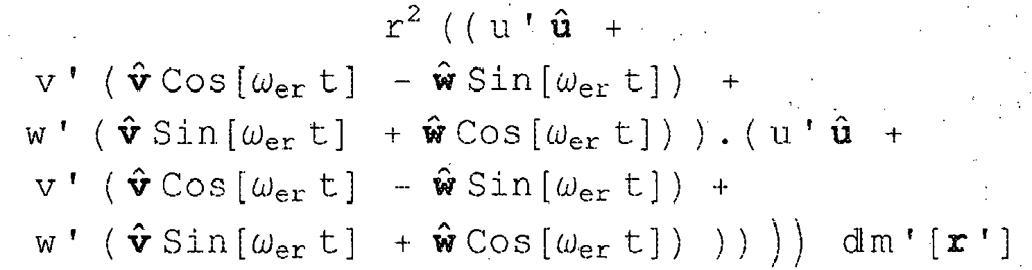
- Simplifying by distributing

- Simplifying the components

- Thus we have


- Substituting back

- Remembering to cancel terms do not contribute because the origin is at the center of gravity

- Remembering to cancel terms involving integrals of (v') 2 and ( w ')2 are equal because of axial syrnetery

- Substituting ( v' )2 by ( w' )2

- Simplifying the trig

- Using

- We get
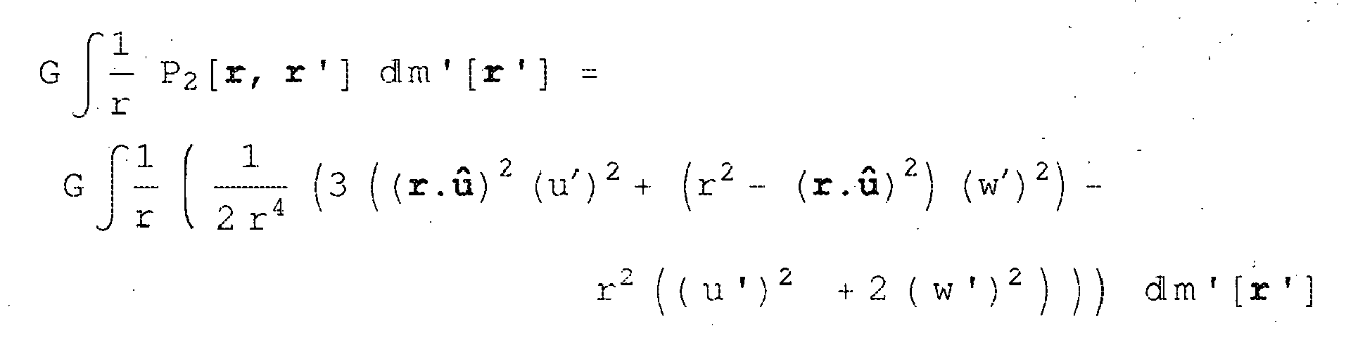
- Distributing we get

- Simplifying we get

- Factoring we get

- Factoring terms independent of r'

- But


- We can rearrange using


- Given axial symmetry, we can express J 2 as above, where J2 has the usual definitions.
- The details of the multipole expansion for an axially symmetric body can be found in
Ref 1. Assuming the body is axial symmetric, a multipole expansion formula for φ[r], independent of coordinate system is


- Such an expansion is then used to calculate the orbits of satellites orbiting round the earth, assuming the earth is axially symmetric, and rotates about its axis of symmetry.
- A more accurate description of the gravitional field is obtained by evaluating the effects due to all the deviations from spherical symmetry. A formula for the earth's potential V, taking all the deviations of the earth from spherical symmetry into account, can be found in Ref 3, and is represented by a spherical harmonic multipole expansion

- We derive, a multipole expansion, similar to the spherical harmonic expansion above, in that we do not assume axial symmetry of the body, but without needing to specify the coordinate system (such as spherical harmonic). It is therefore, valid for bodies that are not axially symmetric. This multipole expansion differs from the multipole expansion found in
reference 1. - The quaternion implementation of the solution to Kepler's equation for predicting orbits is transformed into finding the root by numerical means of an equation, as opposed to numerically solving a non linear differential equation. The quaternion implementation has therefore superior numerical accuracy.
- Quaternions are a subalgebra of geometric algebra and it would be useful to describe the regularising method using geometric algebra. The solution to Kepler's equation in geometric algebra is developed in
Ref 1, but only for axially symmetric bodies. - Now for the general case n. We need to calculate

- Substituting for Pn we have

- Distributing the integral we get

- Using vectors r r̂, r' r̂' for r, and r', where r̂, r̂' are unit vectors we get


- Simplifying

- Expressing the terms involving r' and r a power of

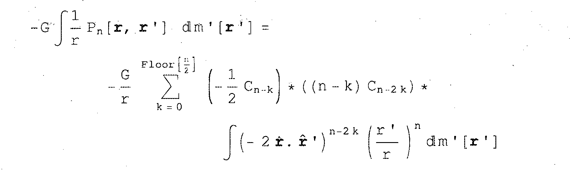
- As in the previous section, let û be a unit vector in the direction of the axis of rotation. Let v̂ and ŵ represent unit vectors orthogonal to û and orthogonal to each other. Then We can express r' as



- And


- And

- Then substituting r.r' and factoring


- Then substituting the values of u,v and w we get

- Expanding the expression raised to the power n-2k, we get

- But

- Factoring and distributing, and interchanging the order of summation with integration, we get


- Expanding, we get

- Distributing


- Factoring under the integral sign

- Factoring under the integral sign

- Simplifying we get


- But


- Substituting we get


- Thus for the earth we have for the nth term of the multipole expansion

- Note that J[n][p, q, r] [û', v̂', ŵ'], are functions of the unit vectors û', v̂', ŵ', and for a particular coordinate system for each p,q, and r , the value of J[n] [p, q, r] [û', v̂', ŵ'] can be determined empirically for the earth, given the trajectories of orbiting satellites.
- We note that we have arrived at the expression to use when we do not wish to assume axial symmetry.
- We write a small program to calculate the first few terms of the multipole expansion. Note that this calculation needs to be done only occassionaly, and so we do not try to optimise the calculation.


- We check with Axial Symmetry

- We check with Axial Symmetry


- We need to calculate the derivative of

- The nth multipole contribution to the force f is given by


- We rearrange the terms that depend on r

- We factor out the terms that do not depend on r


- We have to find the derivative of the following expression

- Replacing unit vector by r

- Simplifying

- Simplifying

- Using the results from Example 9

- Thus

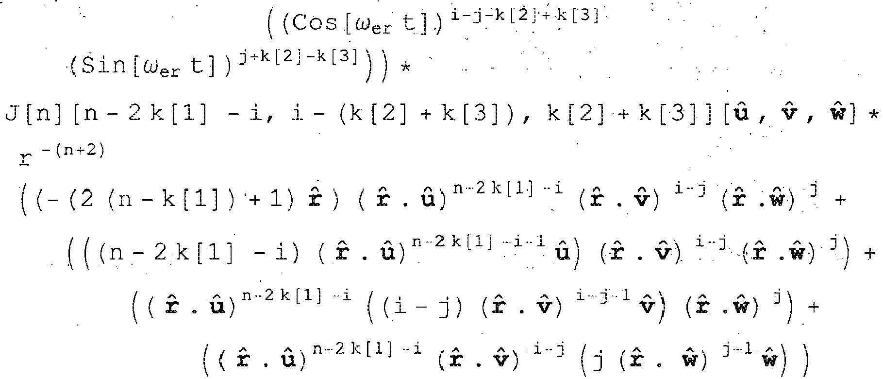
- Rearanging the terms


- Note that when the origin of the coordinate system is at the center of gravity of the body, then J[1] [0, 0, 1] [u, v, ŵ],J[1] [0, 1, 0] [û, v̂, ŵ] and J [1] [1, 0, 0] [û, v̂, ŵ] are zero.
- ForceContributionMultipoleExpansionTerms[2]
- ForceContributionMultipoleExpansionTerms[3]
- ForceContributionMultipoleExpansionTerms[4]
- ForceContributionMultipoleExpansionTerms[5]
- Note that when the system is axially symmetric we can introduce the axiom
J[n_] [a_, b_, c_] [u_, v_, w_] /; c > b := J[n] [a, c, b] [u, v, w]
ForceContributionMultipoleExpansionTerms[3] / / Simplify - We quote some geoid values found
http://geophysics.ou.edu/solid_earth/notes/geoid/earths_geoid.htmTable 2.2 Coefficients of spherical harmonics in the expansion of the gravitational potential of the Earth (a) Zonal harmonics 106 J 2 1082·6 104 J 3 -2·54 J 4 -1·59 J 5 -0·21 J 6 0·50 J 7 -0·40 J 8 -0·12 J 9 0 J 10 -0·35 J 11 0 J 12 -0·04 J 13 0 J 14 -0·07 J 15 -0·20 J 16 0·19 J 17 0 J 18 -0·23 J 19 0 J 21 0·26 (Values from Kozai (1969) and King Hele et al. (1969).) - Let r = r[τ] be the orbit of a particle of unit mass with the Newtoninan equation of motion

- The angular momentum for unit mass is defined as

- It can be shown that L is a bivector

- Proof


- Thus L is a bivector. We get the third equality, from the distributive law, and using the fact

- We next show

- From the unit vector r̂

- We get the first implication by differentiating both sides w.r.t t, and the second implication from the definition of the dot product in geometric algebra.
- Thus we can replace, in L, the outer product ∧, by the geometric product.

- We make appropriate choices for U and σ1 to simplify the geometric algebra equation of motion.
- Given the initial position vector r Init and velocity vector ṙ Init of the orbiting body, we can specify the bivector component of U to be proportional to r̂ Init ∧ r̂ Init i.e.

- We re free to choose σ 1 in the equation for r. We choose σ 1 to be r Init , the unit vector of initial position of the satellite. Then

- Then replacing the outer product ∧, with the geometric product we get

- This implies


- Expressing the above in terms of geometric products we get

- Simplifying, we get

- Taking revision of the second term, we get

- Rearranging, we get

- Also we have for any
scalar 
- Thus we have

- And using reversion,

- We now show, in the sequence below that the subsidary condition is satisfied in a system with these choices of σ1 and U † .

- Substituting for our choice of 〈U〉2

- Distributing

- The equation of motion with U as above and σ 1 = r̂ Init, becomes
- Thus we get the equation of motion in geometric algebra.


- After making the
substitution 


- After making the
substitution 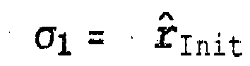


- ▪ Defining

- We need to consider expressions of the following form
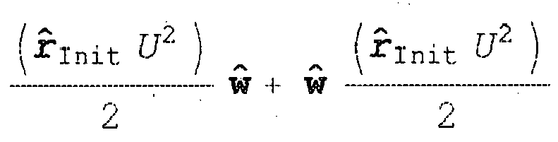
- Let

- Then

- Expanding

- Using


- Thus we get

- Distributing we get

- Thus we get

- Finally

- Define


- We divide ((β2 - α2) r̂ Init .ŵ + 2αβ ṙ Init .ŵ) by rInit in order to maintain precision. This is new
- ▪ Equation of Motion in terms of

- Simplifying by substituting


- Factoring


- Factoring


- But

- Thus

- Thus the equation of motion becomes


- ▪ Expanding

- As long as 2 r init> r


- By making the substion


- Let


- We note that Γ n [U, û, v̂, ŵ, r̂ Init, ṙ Init] also depends on the constants multipole constants, J [n] [p, q, r] [û, v̂, ŵ]. Once the unit vectors û, v̂, ŵ have been fixed, J[n] [p, q, r] [û, v̂, ŵ] is a constant.
- For each n, Γ n [U, û, v̂, ŵ, r̂ Init, ṙ Init need only be calculated once, to yield a function in terms of U, given the initial position r Init, and initial velocity ṙ Init, and the unit vectors û, v̂, ŵ, as Γ n [U, û, v̂, ŵ, r̂ Init, ṙ Init] then just depends on U, the rest of the inputs being constant.
- The expression for the equation of motion,

-

- Integrating

- When U[s] is of the form

- Distributing

- When Ui [s] is of the form

- Where αi,j, βi,j and ωi,j do not depend on s, and βi,j is a 2-blade independent of s, and all the βi,j lie in the same plane and λU
i is the number of distinct frequencies that ωi,j that constitute Ui[s].Then
- Distributing and integrating and assuming all the bivectors lie in the same plane

- The above expression can be expressed as

- We can therefore express t as a linear combination of distinct exponential frequencies after simplification

- ▪ Getting the perturbed version of


- When


- Then

- Then


- Distributing and factoring

- Changing the order of the summation

- Define

- Then


- ▪ Getting the perturbed version of


- Substituting


- Define

- A computer algebra system may be used to calculate the functions rather than doing this manually.

- We demonstrate the perturbation method by generating the the first three (up to and equal to 2nd Order) using
standard perturbation theory 
- The above equation is an example of a weakly non-linear equation to which one may apply perturbation techniques e.g Lindstedt-Poincare (Ref 4) to generate analytic solutions correct to a given order. Vrbik (Ref 8) has produced perturbed solutions to orbits using quaternion.
- We proceed to demonstrate the method
- Let

- And let

- And let

- Where

- Then we get for the equation of
motion 
- Substituting for E and

motion 
- Substituting for

motion 
- Rearranging the summation we get for the equation of
motion 
- Factoring we get for the equation of motion

- We have shown that we can express t as a linear combination of distinct exponential frequencies.

- Using a Taylor's expansion for Sin we can get the following series

- Where λSin , and λcos are the number of terms to use for the desired accuracy and j is complex square root of -1.
- We can thus put this expression into the form

- And

- Where λSin, i, and λcos, i are the number of exponentialsgenerated for the desired accuracy.

- ▪ Approximating

- Thus the solution to 0th order equaton is given by

- Substituting the initial values into the solution

- We show further on that

- Thus

- Now

- This simplifies to

- Unfolding we get

- Thus

- Thus we get

- We therefore have

- Where

- The
quantity 

- Thus it is valid to use the
approximation 
- The expression is thus a sum of exponential functions

- For positive n

- We deal with negative n in the following way

- Let the last term of this series to be used be denoted

- The number of terms to use depends on the orbit of the satellite. When the encentricity of the orbit is small, then only a few terms need be used. For satellite orbits which are nearly circular, then only as few as 4 terms may be sufficient. Also, if it is possible to select the initial position, then select the position that is approximately the square root of the product of the nearest and furtherst distances.

- We can therefore put this expression in the form

- ▪ Expressing

- We have defined


- When U can be expressed as


- This may be simplified to
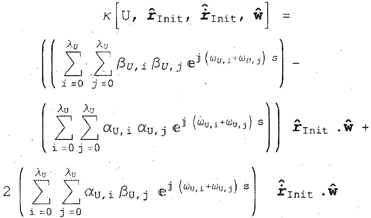
- There may be some frequencies in the above expression that may occur more than once. The expression can therefore be put in the form

- We have shown that

- Let

- Then

- Thus we can express


- ▪ Expressing

- We have shown that


 in the ith perturbation
- The perturbed equation of motion is given by

- The constraints on ω

- The initial condition on position

- This simplifies to

- Thus

- Where we regard Ui as a function of s

- Let

- The initial condition on velocity

- Therefore,

- Substituting for r

- Rearranging the summations

- Ignoring O(∈)


- Ignoring O (∈2)
- The perturbed equation of motion is given by

- Ignoring

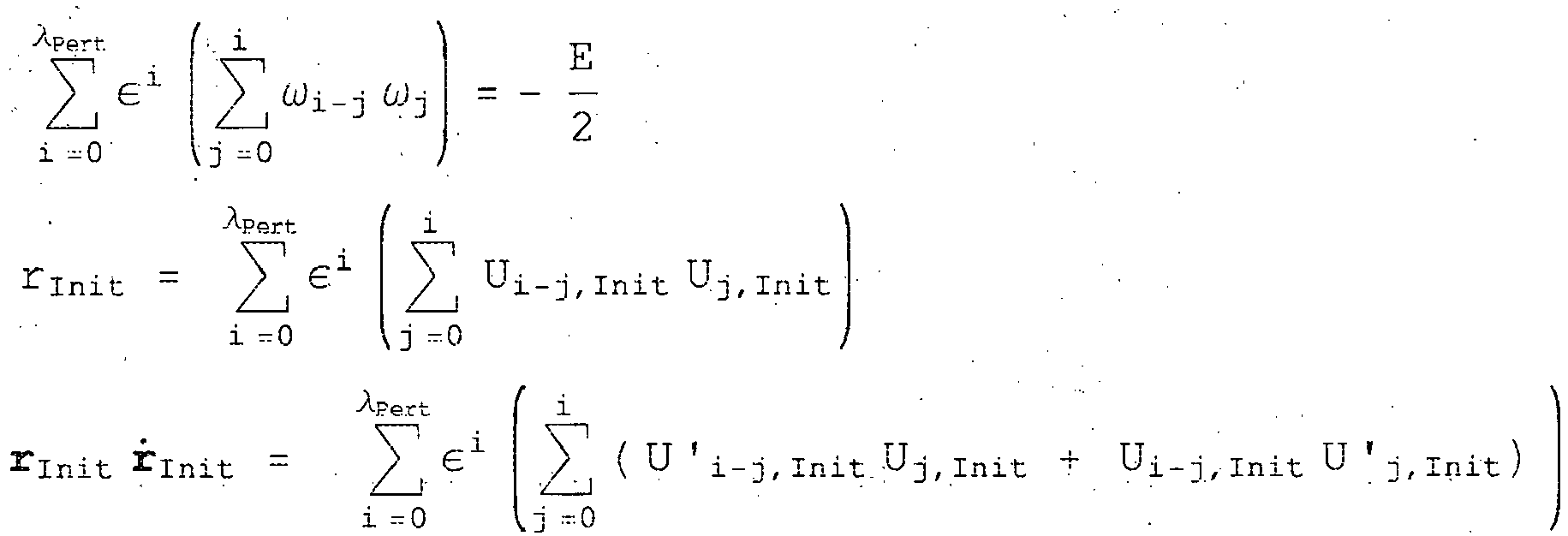
- The solutions to these equation of motion of the orbiting satellite of different order are uniquely determined correct to a the accuracy of approximation given the initial position, r Init , and initial velocity, ṙ Init, of the orbiting satellite by a deterministic expression. Details of how to convert the initial position vector and the initial velocity of the satellite are shown next
- An equation of the form


- If for some i


- Consider


- This particular solution is unstable because x[s] tends to ∞ as s tends to ∞. Thus for stable solutions, we have for i, such that

- In this section we assume that the constants

- We show next, how to calculate the unique solution to this equation of motion of the orbiting satellite correct to the accuracy of approximation required given the initial position and velocity of the orbiting satellite by a deterministic expression.
- An equation of the form


- If for some i

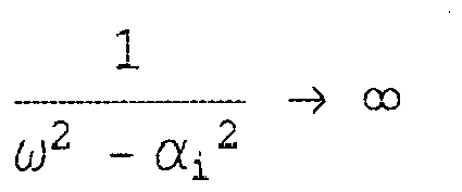
- Consider


- This particular solution is unstable because x[s] tends to ∞ as s tends to ∞. Thus for stable solutions, we have for i, such that

- The 0th order equaton is given by


- We have shown before that

- And

- Thus the solution to 0th order equaton is given by

- Substituting the initial values into the solution

- The first order equation becomes

- This simplifies to


- This can be expressed as

- And
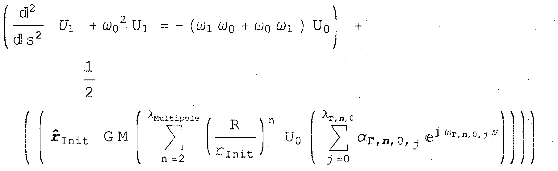
- We thus have a system of two differential equations. The general solution from the first equation


- The right hand side of the second equation can be expressed as a sum of exponentials
- The coefficient of the exponential


- Applying the stability condition we get a value for ω1

- Note we would get the same walue for ω1 if we considered the coefficient of the exponential

- Substituting this value of ω1 into the equation we get a differential equation for U 1, where the right hand side is entirely in terms of a, b, and ω0. We can therefore calculate the particular solution of U 1.
- Note, by construction, the particular solution of U 1 is stable.
- We can proceed finding ω2, U 2, ω3, U 3, ω4, U 4, ... .. up to the desired level of perturbation We have shown that

order 1 accuracy.
- We will demonstrate the next stage of the method using the first order perterbation equation

- By substituting the value of ω1 into the equation that constrains ω

- By substituting the value of U 0[0|, U 1[0] into the initial position equation
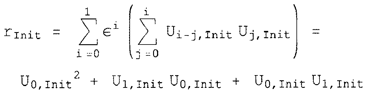
- We can calculate U'0[s ] and U'1[ s ] in terms of terms of a, b, ω0 and s.
- By substituting the solution of U 0[0], U 1[0], U'0[0] and U'1[0] into

- We now have a situation where we have three unknowns a, b, ω0. and three equations(the 3 boundary conditions). We can solve for these three equations for the 3 ubknowns using any of the standard methods such as FletcherPowel algorithm
- We can substitute the values of a,b, and ω0 into


- Now we can put


† ,i represents the number of exponentials required to represent the contribution of the ith perterbation component - Note that αU U
† , i, j and ωU U† ,i, j can be precalculated in terms of a,b, and ω0
- One needs to evaluate the following equation in order to get the position of satellite.

- One can simplify the expression for t to the form of
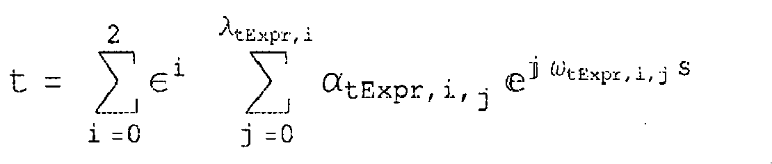
- To get the nth order solution,
- 1)WorkingOrder = 0
- 2) U0 = Solution of differential equation of order 0 in terms of the unknowns a,b, and ω0.
- 3)WorkingOrder =
WorkingOrder + 1; - 4) DiffEqWorkingOrder= Substitute U WorkingOrder-1 into the differential equation for (WorkingOrder).
- 5) Solve for ωWorkingOrder using the stability condition on DiffEqWorkingOrder (Note that ωWorkingOrder is in terms of the unknowns a,b, and ω0.) Store ωWorkingOrder.
- 6) SolvableDiffEqWorkingOrder = Substitute ωWorkingOrder into DiffEqWorkingOrder
- 7) U WorkingOrder = Particular Solution of SolvableDiffEqWorkingOrder.(Note that U WorkingOrder is in terms of the unknowns a,b, and ω0.) StoreU WorkingOrder.
- 8) If WorkingOrder = n, goto 9 else goto 3
- 9) Substitute the values of ω1, ω2, ω3,...ωn and U0, U1, U 2, U3, ... Un into the constraint equation and initial condition equations, to get 3 equations connecting the initial conditions with a,b and ω0.
- 10) Solve equations in step 9 to get values of a,b, and ω0 in terms of the initial conditions only.
- 11) Substitute values from 10 into U0, U1, U2, U3, ... Un to get U0, U1, U2, U3, ... Un in terms of the initial conditions.
- One needs to solve the following equation in order to get the position of satellite at time t 1 given the initial conditions at time t 0. We have shown before that

- Let Ξ[k], where

- Ξ[k], is a non-linear equation, for k>1, and entirely in terms of the initial conditions once we have solved for a,b, and ω0. One of the methods of solving it would be to get an estimate of s 1, using, Ξ[0], the zero order perturbation equation, then using the solution of Ξ[0] as initial input for Newton-Raphson method for solving Ξ[1], and so on until one arrives at the solution for the appropriate equation to be solved.
- Afrer solving the above equation where s 1 is the only unknown we can calculate the position using

- One can set up equations involving J[n] [p, q, r] [û, v̂, ŵ], if the positions, r t
i , of a satellite are known accurately at different times ti . Let si be the associated value with ti, where s i is unknown but {ti,r ti , si} can be substituted into the following pair of equations for each i
- And

- We also have the three equations linking the initial conditions with the unknowns a,b, and ω0.
- The unknowns in all these equations are J [n] [p, q, r][û, v̂, ŵ] and the si and a,b, and ω0.
- One needs at least one point for each J [n] [p, q, r] [û, v̂, ŵ] that is unknown. If there are several points, then these equations can be solved using least mean squared techniques to increase the accuracy with which the J [n] [p, q, r] [û, v̂, ŵ] are determined. Also, several different satellites can be used to increase the accuracy of the solutions to the constants J [n] [p, q, r] [û, v̂, ŵ].
- In the section above, we have shown that all the steps detailed below can be carried out routinely.
- For some given time, t 0 we know the position of the position of the satellite and its velocity.
- Suppose we wish to calculate the position of the satellite at some other time t 1 where t 1 > t 0
- Then
- 1) we use the position and velocity to calculate U 0 and
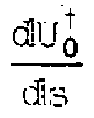


- 2) Calculate t 1 - t 0
- 3) Calculate the equations for U 0, U 1, U 2, U 3, ... Un in terms of unknowns a,b and ω0, and store in a lookup table.
- 4) Calculate the equation

- 5) Calculate the three equations connecting the initial conditions and the constraints on ω in terms of the unknowns unknowns a,b and ω0, and the initial conditions r Init, ṙ Init. (It is possible to calculate these equations in terms of 5 unknowns a,b, ω0, r Init, ṙ Init in advance and stored. When r Init, ṙ Init become known, these values are stored in the equations)
- 6) Solve the 3 equations in step 5) to get values for a,b, and ω0
- 7)Substitute these values in the stored equations for U0, U1, U2, U3, ... Un in step 3)
- 8) Substitute in equation calculated in step 4), the values of a,b, and ω0 and t = t 1 the time at which the position is to be determined and solve the resulting equation for s. Say the solution to the equation is s = S 1
- 9)Use r t
1 = U † [S1 ] r̂ Init u [S1] to calculate the position of the orbit at time t 1 - We also notice, that the accuracy of the solution is determined by the factors included in the pertubation forces. The solution does not deteriorate with time. The solution is expressed in terms exponential functions.
- We need to be able to work out the geometric derivative for some standard formulae The Product Rule

- But the limit of a sum is the sum of the individual limits

- The first limit can be expressed as two limits, because interchanging the order of the limits yields the same limit point.

- Using the notation in Hestenes

- Thus we have

- The equivalent of chain rule
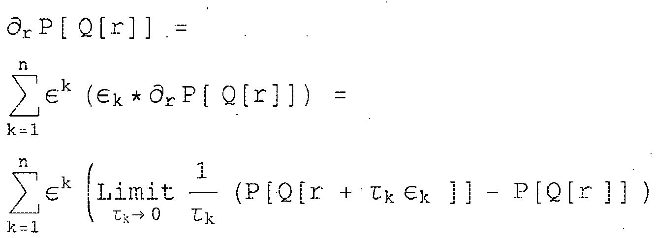
- But we can express by Taylor's theorem

- Substituting we have

- But the expression


- And

- Because of linearity we have

- Thus we have

- The derivative of a power. True only for a scaler, which commutes

- Multiplying the brackets we get

- We can factor

- But


- The derivative of a power Continued

- If P[r] = < P[r] >0, then

- Thus

- For
-

- We cannot apply the power rule to ∂r (r 2). However, from first principles, we have

-

-

- But
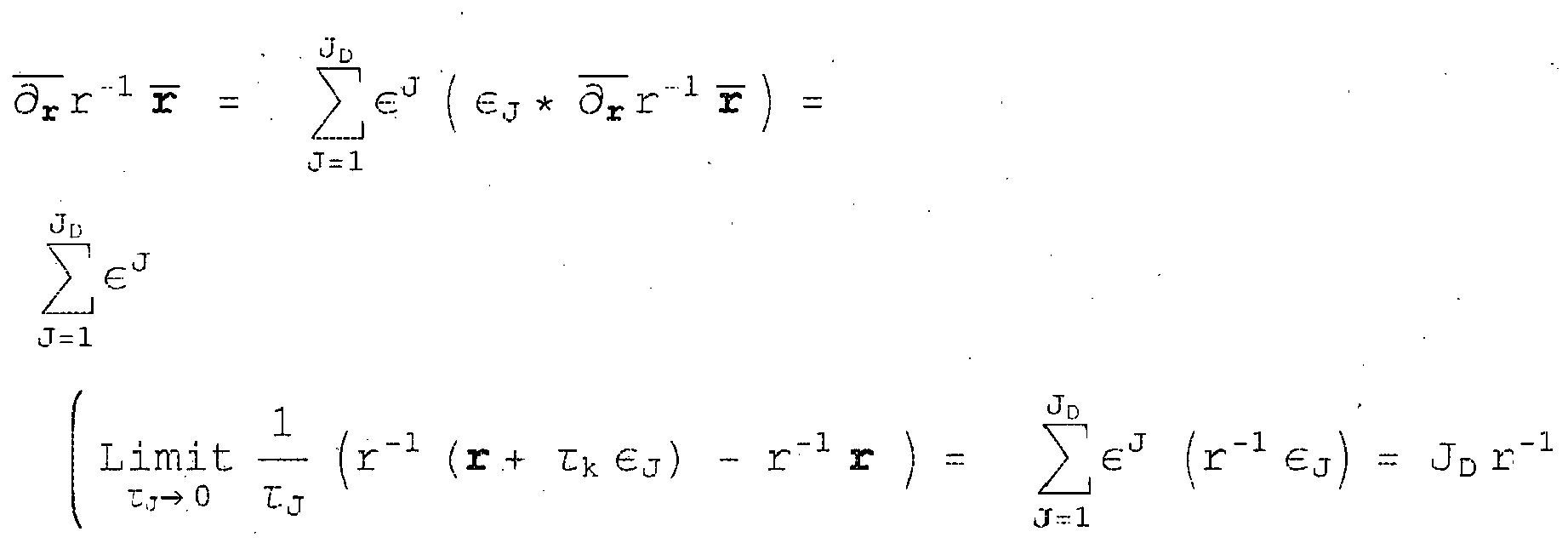
- Thus

- is an interesting.


- From first principles ∂ r r u

- From first principles ∂ r u r

- Exchanging the order of summation we get

- But the vectors ∈J ∈K anti- commute and ∈K ∈K = 1


-

- Using the product rule we get

- When we do ∂ r (r̂ . u) from first principles we also get

-

- By the product rule

-

-

- We have to find the derivative of the following expression

- Replacing unit vector by r

- Simplifying

- Simplifying

-

- Using Hestenes overbar notation and the product rule
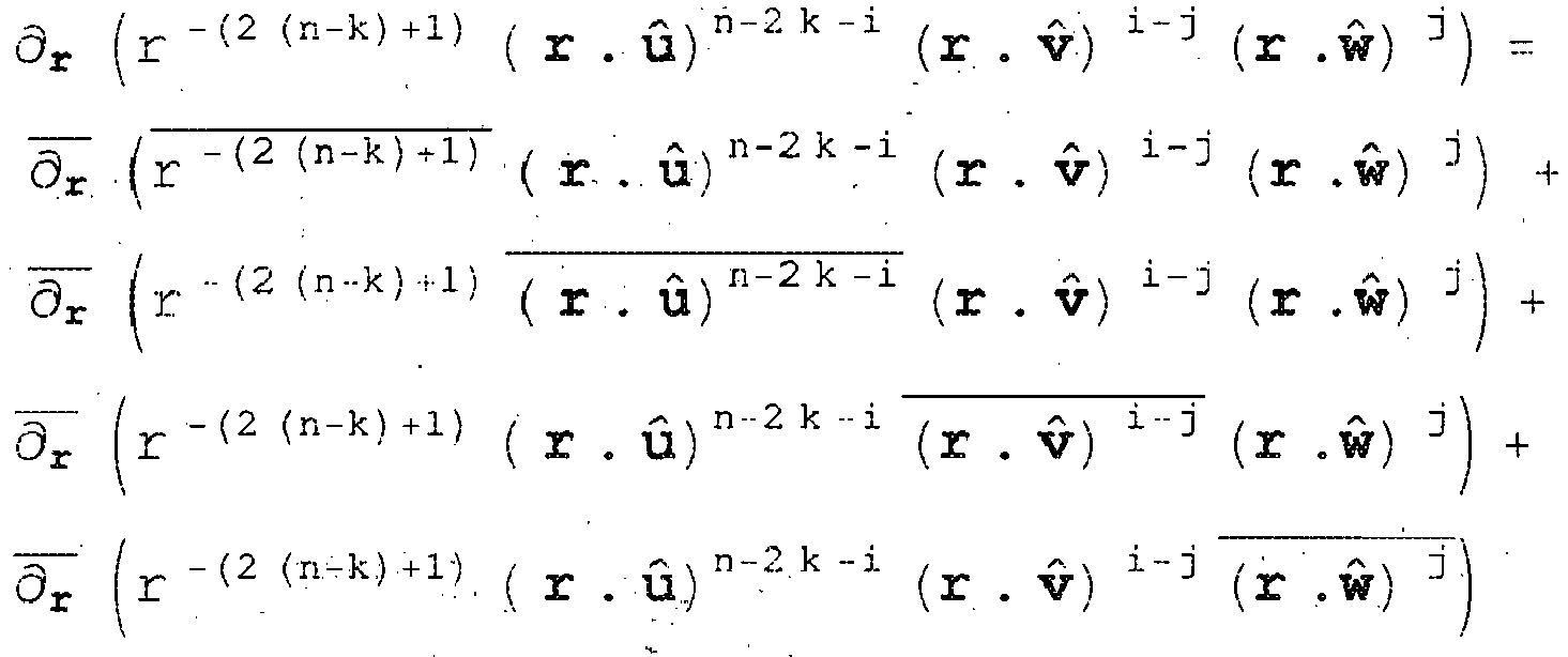
- As all the terms differentiated are sealers, the expressions commute and so we can factor the active sub expressions
-

-

-

-

- Substituting the results of the above

- Simplifying in terms of unit vectors

- Simplifying we get

- We assume i,j,k are mutially orthogonal unit vectors. The rules below have been implemented in Mathematica to generate the geometric product of two geometric algebra multivectors


-
- 1 Hestenes David, "New Foundations for Classical Mechanics (Second Edition)", Kluwer Academic Publishers
- 2 Hestenes David and Sobczyk Garret, "Clifford Algebra to Geometric Calculus", Kluwer Academic Publishers
- 3 Hofmann-Wellenhof B., Lichtenegger H., and Collins J., "GPS Theory and Practice", Fourth, revised edition, Springer Wien, New York
- 4 Drazin P. G., "Nonlinear Systems", Cambridge Texts in Applied Mathematics
- 5 Waldvogel Jorg, "Quaternions for Regularizing Celestial Mechanics- the Right Way, Research Report No. 2009-09, May 2008, ETH Switzerland
- 6 Vrbik, Jan, "Perturbed Kepler problem in quaternionic form". J. Phys. A 28, 193-198. (1995)
- 7 Bartsch T., "The Kustaanheimo-Stiefel transformation in geometric algebra", arXiv:-physics/0301017v1[physics.class-ph] 10 Jan 2003
- 8 Vrbik Jan, "Kepler problem with time-dependent and resonant perturbations", Journal of Methematical Physics 48, 052701 (2007)
Claims (15)
- A method in a receiver apparatus configured to receive positioning signals from Global Navigation Satellite System (GNSS) satellites (2),
comprising:positioning the receiver apparatus at a time value by, for each of a plurality of GNSS satellites:using an algebraic solution of a differential equation of motion of the GNSS satellite to determine a position of the GNSS satellite at the time value andusing positioning signals received at the receiver apparatus at the time value from the GNSS satellite. - A method as claimed in claim 1, wherein using an algebraic solution of a differential equation of motion of the GNSS satellite to determine a position of the GNSS satellite at the time value comprises using pre-calculated algebraic look-up.
- A method as claimed in claim 2, comprising using nested look-up tables for multiple different constellations of GNSS satellites.
- A method as claimed in claim 1, comprising:having received, for each of the plurality of the GNSS satellites (2), first information for defining a first algebraic function that relates a time variable to a first mapped variable,performing long-term-accurate-positioning of each of the plurality of the GNSS satellites (2) without the need for receiving updated ephemeris data by:using the first information defining the first algebraic function to convert (40) the time value of the time variable to a first value of the first mapped variable;converting (41) the first value of the first mapped variable to a second value of a second mapped variable; andpositioning (42) the GNSS satellite by converting the second value of the second mapped variable to a position value that positions the GNSS satellite (2) at the time value.
- A method as claimed in claim 4, wherein the first algebraic function is based upon an algebraic solution to a geometric algebraic differential equation of motion of a GNSS satellite.
- A method as claimed in claim 4 or 5, wherein the first information includes coefficients for defining the first algebraic function
- A method as claimed in any of claims 4 to 6, wherein a second algebraic function that relates the first mapped variable to the second mapped variable is used to convert the first value of the first mapped variable to a second value of a second mapped variable.
- A method as claimed in claim 7, wherein the second algebraic function is an algebraic solution to the differential equation of motion of the satellite.
- A method as claimed in claim 7 or 8, further comprising receiving second information for defining the second algebraic function.
- A method as claimed in claim 9, wherein the second information includes coefficients for defining the second algebraic function.
- A method as claimed in any one of claims 7 to 11, wherein the first and second algebraic functions are expressed using complex exponential functions.
- A method as claimed in any of claims 7 to 11, wherein the differential equation of motion is

whereE is a constantU is the second mapped variable and is defined by r = U + σ 1 U σ 1 has a constant unit lengths is the first mapped variable and is defined by f is expressed using geometric algebra in terms of U.
 - A method as claimed in any preceding claim, wherein the method of the preceding claim is always performed after the receiver apparatus has been switched on using prestored first information.
- An apparatus comprising means for performing the method of any of claims 1 to 13.
- A computer program comprising instructions which when loaded into a processor enable the processor to: for perform the method of any of claims 1 to 13.
Priority Applications (1)
| Application Number | Priority Date | Filing Date | Title |
|---|---|---|---|
| EP14191355.8A EP2843442B1 (en) | 2009-12-22 | 2009-12-22 | Positioning satellites |
Applications Claiming Priority (3)
| Application Number | Priority Date | Filing Date | Title |
|---|---|---|---|
| EP09796387.0A EP2517047B1 (en) | 2009-12-22 | 2009-12-22 | Positioning satellites |
| EP14191355.8A EP2843442B1 (en) | 2009-12-22 | 2009-12-22 | Positioning satellites |
| PCT/EP2009/067782 WO2011076260A1 (en) | 2009-12-22 | 2009-12-22 | Positioning satellites |
Related Parent Applications (2)
| Application Number | Title | Priority Date | Filing Date |
|---|---|---|---|
| PCT/EP2009/067782 Previously-Filed-Application WO2011076260A1 (en) | 2009-12-22 | 2009-12-22 | Positioning satellites |
| EP09796387.0A Division EP2517047B1 (en) | 2009-12-22 | 2009-12-22 | Positioning satellites |
Publications (3)
| Publication Number | Publication Date |
|---|---|
| EP2843442A2 true EP2843442A2 (en) | 2015-03-04 |
| EP2843442A3 EP2843442A3 (en) | 2015-05-13 |
| EP2843442B1 EP2843442B1 (en) | 2019-07-31 |
Family
ID=42470584
Family Applications (3)
| Application Number | Title | Priority Date | Filing Date |
|---|---|---|---|
| EP14191355.8A Not-in-force EP2843442B1 (en) | 2009-12-22 | 2009-12-22 | Positioning satellites |
| EP09796387.0A Not-in-force EP2517047B1 (en) | 2009-12-22 | 2009-12-22 | Positioning satellites |
| EP14191319.4A Not-in-force EP2878973B1 (en) | 2009-12-22 | 2009-12-22 | Positioning satellites |
Family Applications After (2)
| Application Number | Title | Priority Date | Filing Date |
|---|---|---|---|
| EP09796387.0A Not-in-force EP2517047B1 (en) | 2009-12-22 | 2009-12-22 | Positioning satellites |
| EP14191319.4A Not-in-force EP2878973B1 (en) | 2009-12-22 | 2009-12-22 | Positioning satellites |
Country Status (3)
| Country | Link |
|---|---|
| US (1) | US8843251B2 (en) |
| EP (3) | EP2843442B1 (en) |
| WO (1) | WO2011076260A1 (en) |
Families Citing this family (4)
| Publication number | Priority date | Publication date | Assignee | Title |
|---|---|---|---|---|
| GB2483713B (en) * | 2010-09-20 | 2016-04-06 | St Microelectronics Res & Dev | Signal verification |
| US10761739B2 (en) * | 2018-08-23 | 2020-09-01 | Micron Technology, Inc. | Multi-level wear leveling for non-volatile memory |
| US11537307B2 (en) | 2018-08-23 | 2022-12-27 | Micron Technology, Inc. | Hybrid wear leveling for in-place data replacement media |
| CN109823571B (en) * | 2019-01-23 | 2020-07-03 | 清华大学 | A multi-stage attitude control method for remote sensing micro-nano satellites |
Family Cites Families (5)
| Publication number | Priority date | Publication date | Assignee | Title |
|---|---|---|---|---|
| US6138061A (en) * | 1997-04-18 | 2000-10-24 | Hughes Electronics Corporation | Onboard orbit propagation using quaternions |
| US6337657B1 (en) * | 1999-03-12 | 2002-01-08 | Topcon Positioning Systems, Inc. | Methods and apparatuses for reducing errors in the measurement of the coordinates and time offset in satellite positioning system receivers |
| EP1852711B1 (en) * | 2006-04-24 | 2013-03-13 | Qualcomm Incorporated | Ephemeris extension method for GNSS applications |
| US7564406B2 (en) * | 2006-11-10 | 2009-07-21 | Sirf Technology, Inc. | Method and apparatus in standalone positioning without broadcast ephemeris |
| US8099186B2 (en) * | 2006-12-22 | 2012-01-17 | The Boeing Company | Satellite navigation using long-term navigation information and autonomous orbit control |
-
2009
- 2009-12-22 EP EP14191355.8A patent/EP2843442B1/en not_active Not-in-force
- 2009-12-22 WO PCT/EP2009/067782 patent/WO2011076260A1/en not_active Ceased
- 2009-12-22 US US13/517,027 patent/US8843251B2/en not_active Expired - Fee Related
- 2009-12-22 EP EP09796387.0A patent/EP2517047B1/en not_active Not-in-force
- 2009-12-22 EP EP14191319.4A patent/EP2878973B1/en not_active Not-in-force
Non-Patent Citations (8)
| Title |
|---|
| BARTSCH T.: "The Kustaanheimo-Stiefel transformation in geometric algebra", ARXIV:-PHYSICS/0301017VL[PHYSICS.CLASS-PH, 10 January 2003 (2003-01-10) |
| DRAZIN P. G.: "Nonlinear Systems", CAMBRIDGE TEXTS IN APPLIED MATHEMATICS |
| HESTENES DAVID: "New Foundations for Classical Mechanics (Second Edition", KLUWER ACADEMIC PUBLISHERS |
| HESTENES DAVID; SOBCZYK GARRET: "Clifford Algebra to Geometric Calculus", KLUWER ACADEMIC PUBLISHERS |
| HOFMANN-WELLENHOF B.; LICHTENEGGER H.; COLLINS J.: "GPS Theory and Practice", SPRINGER |
| VRBIK JAN: "Kepler problem with time-dependent and resonant perturbations", JOURNAL OF METHEMATICAL PHYSICS, vol. 48, 2007, pages 052701 |
| VRBIK, JAN: "Perturbed Kepler problem in quatemionic form", J. PHYS. A, vol. 28, 1995, pages 193 - 198 |
| WALDVOGEL JORG: "Research Report No. 2009-09", May 2008, ETH, article "Quaternions for Regularizing Celestial Mechanics- the Right Way" |
Also Published As
| Publication number | Publication date |
|---|---|
| EP2517047A1 (en) | 2012-10-31 |
| EP2878973B1 (en) | 2019-01-30 |
| EP2843442B1 (en) | 2019-07-31 |
| US20120253563A1 (en) | 2012-10-04 |
| US8843251B2 (en) | 2014-09-23 |
| EP2878973A1 (en) | 2015-06-03 |
| EP2517047B1 (en) | 2014-11-26 |
| WO2011076260A1 (en) | 2011-06-30 |
| EP2843442A3 (en) | 2015-05-13 |
Similar Documents
| Publication | Publication Date | Title |
|---|---|---|
| Müller et al. | High performance clocks and gravity field determination | |
| Taylor et al. | Putting the Precision in Precision Cosmology: How accurate should your data covariance matrix be? | |
| Milani et al. | Testing general relativity with the BepiColombo radio science experiment | |
| Armellin et al. | Asteroid close encounters characterization using differential algebra: the case of Apophis | |
| Vines et al. | First-post-Newtonian quadrupole tidal interactions in binary systems | |
| Millea et al. | Bayesian delensing of CMB temperature and polarization | |
| Pettinari et al. | The intrinsic bispectrum of the Cosmic Microwave Background | |
| Vecchiato et al. | Testing general relativity by micro-arcsecond global astrometry | |
| Giri et al. | Exploring KSZ velocity reconstruction with N-body simulations and the halo model | |
| Giblin Jr et al. | General relativistic corrections to the weak lensing convergence power spectrum | |
| EP2517047B1 (en) | Positioning satellites | |
| Liu et al. | Initial orbit determination of periodic orbits in the earth–moon system with ground-based optical observations | |
| Chen et al. | Autonomous navigation using X-ray pulsars and multirate processing | |
| US20150285919A1 (en) | Positioning satellites | |
| Page et al. | Bayesian time delay interferometry for orbiting LISA: Accounting for the time dependence of spacecraft separations | |
| Tommei et al. | Light-time computations for the BepiColombo radio science experiment | |
| Dimitrov | Elliptic integrals for calculation of the propagation time of a signal, emitted and received by satellites on one orbit | |
| Weisman et al. | Solution of Liouville's Equation for Uncertainty Characterization of the Main Problem in Satellite Theory | |
| Folcik et al. | Reconciling covariances with reliable orbital uncertainty | |
| Folkner | Relativistic aspects of the JPL planetary ephemeris | |
| Woodburn et al. | Effect of coordinate selection on orbit determination | |
| Pardal et al. | An investigation on cubature Kalman filter performance for orbit determination application | |
| Peron | Testing general relativistic predictions with the LAGEOS satellites | |
| Craft et al. | Performance Determination of a Multi-Mode Thruster Using GPS and Star Tracker Data | |
| Yu | Characterization of X-ray pulsar navigation for tracking closed Earth orbits |
Legal Events
| Date | Code | Title | Description |
|---|---|---|---|
| 17P | Request for examination filed |
Effective date: 20141031 |
|
| AC | Divisional application: reference to earlier application |
Ref document number: 2517047 Country of ref document: EP Kind code of ref document: P |
|
| AK | Designated contracting states |
Kind code of ref document: A2 Designated state(s): AT BE BG CH CY CZ DE DK EE ES FI FR GB GR HR HU IE IS IT LI LT LU LV MC MK MT NL NO PL PT RO SE SI SK SM TR |
|
| PUAI | Public reference made under article 153(3) epc to a published international application that has entered the european phase |
Free format text: ORIGINAL CODE: 0009012 |
|
| PUAL | Search report despatched |
Free format text: ORIGINAL CODE: 0009013 |
|
| AK | Designated contracting states |
Kind code of ref document: A3 Designated state(s): AT BE BG CH CY CZ DE DK EE ES FI FR GB GR HR HU IE IS IT LI LT LU LV MC MK MT NL NO PL PT RO SE SI SK SM TR |
|
| RIC1 | Information provided on ipc code assigned before grant |
Ipc: G01S 19/27 20100101AFI20150409BHEP |
|
| R17P | Request for examination filed (corrected) |
Effective date: 20151111 |
|
| RBV | Designated contracting states (corrected) |
Designated state(s): AT BE BG CH CY CZ DE DK EE ES FI FR GB GR HR HU IE IS IT LI LT LU LV MC MK MT NL NO PL PT RO SE SI SK SM TR |
|
| RAP1 | Party data changed (applicant data changed or rights of an application transferred) |
Owner name: NOKIA TECHNOLOGIES OY |
|
| 17Q | First examination report despatched |
Effective date: 20160504 |
|
| GRAP | Despatch of communication of intention to grant a patent |
Free format text: ORIGINAL CODE: EPIDOSNIGR1 |
|
| STAA | Information on the status of an ep patent application or granted ep patent |
Free format text: STATUS: GRANT OF PATENT IS INTENDED |
|
| INTG | Intention to grant announced |
Effective date: 20180307 |
|
| GRAJ | Information related to disapproval of communication of intention to grant by the applicant or resumption of examination proceedings by the epo deleted |
Free format text: ORIGINAL CODE: EPIDOSDIGR1 |
|
| STAA | Information on the status of an ep patent application or granted ep patent |
Free format text: STATUS: EXAMINATION IS IN PROGRESS |
|
| INTC | Intention to grant announced (deleted) | ||
| GRAS | Grant fee paid |
Free format text: ORIGINAL CODE: EPIDOSNIGR3 |
|
| STAA | Information on the status of an ep patent application or granted ep patent |
Free format text: STATUS: GRANT OF PATENT IS INTENDED |
|
| GRAP | Despatch of communication of intention to grant a patent |
Free format text: ORIGINAL CODE: EPIDOSNIGR1 |
|
| INTG | Intention to grant announced |
Effective date: 20190225 |
|
| GRAA | (expected) grant |
Free format text: ORIGINAL CODE: 0009210 |
|
| STAA | Information on the status of an ep patent application or granted ep patent |
Free format text: STATUS: THE PATENT HAS BEEN GRANTED |
|
| AC | Divisional application: reference to earlier application |
Ref document number: 2517047 Country of ref document: EP Kind code of ref document: P |
|
| AK | Designated contracting states |
Kind code of ref document: B1 Designated state(s): AT BE BG CH CY CZ DE DK EE ES FI FR GB GR HR HU IE IS IT LI LT LU LV MC MK MT NL NO PL PT RO SE SI SK SM TR |
|
| REG | Reference to a national code |
Ref country code: GB Ref legal event code: FG4D Ref country code: CH Ref legal event code: EP |
|
| REG | Reference to a national code |
Ref country code: AT Ref legal event code: REF Ref document number: 1161510 Country of ref document: AT Kind code of ref document: T Effective date: 20190815 |
|
| REG | Reference to a national code |
Ref country code: IE Ref legal event code: FG4D |
|
| REG | Reference to a national code |
Ref country code: DE Ref legal event code: R096 Ref document number: 602009059331 Country of ref document: DE |
|
| RAP2 | Party data changed (patent owner data changed or rights of a patent transferred) |
Owner name: NOKIA TECHNOLOGIES OY |
|
| REG | Reference to a national code |
Ref country code: NL Ref legal event code: FP |
|
| REG | Reference to a national code |
Ref country code: LT Ref legal event code: MG4D |
|
| REG | Reference to a national code |
Ref country code: AT Ref legal event code: MK05 Ref document number: 1161510 Country of ref document: AT Kind code of ref document: T Effective date: 20190731 |
|
| PG25 | Lapsed in a contracting state [announced via postgrant information from national office to epo] |
Ref country code: HR Free format text: LAPSE BECAUSE OF FAILURE TO SUBMIT A TRANSLATION OF THE DESCRIPTION OR TO PAY THE FEE WITHIN THE PRESCRIBED TIME-LIMIT Effective date: 20190731 Ref country code: LT Free format text: LAPSE BECAUSE OF FAILURE TO SUBMIT A TRANSLATION OF THE DESCRIPTION OR TO PAY THE FEE WITHIN THE PRESCRIBED TIME-LIMIT Effective date: 20190731 Ref country code: FI Free format text: LAPSE BECAUSE OF FAILURE TO SUBMIT A TRANSLATION OF THE DESCRIPTION OR TO PAY THE FEE WITHIN THE PRESCRIBED TIME-LIMIT Effective date: 20190731 Ref country code: AT Free format text: LAPSE BECAUSE OF FAILURE TO SUBMIT A TRANSLATION OF THE DESCRIPTION OR TO PAY THE FEE WITHIN THE PRESCRIBED TIME-LIMIT Effective date: 20190731 Ref country code: PT Free format text: LAPSE BECAUSE OF FAILURE TO SUBMIT A TRANSLATION OF THE DESCRIPTION OR TO PAY THE FEE WITHIN THE PRESCRIBED TIME-LIMIT Effective date: 20191202 Ref country code: BG Free format text: LAPSE BECAUSE OF FAILURE TO SUBMIT A TRANSLATION OF THE DESCRIPTION OR TO PAY THE FEE WITHIN THE PRESCRIBED TIME-LIMIT Effective date: 20191031 Ref country code: SE Free format text: LAPSE BECAUSE OF FAILURE TO SUBMIT A TRANSLATION OF THE DESCRIPTION OR TO PAY THE FEE WITHIN THE PRESCRIBED TIME-LIMIT Effective date: 20190731 Ref country code: NO Free format text: LAPSE BECAUSE OF FAILURE TO SUBMIT A TRANSLATION OF THE DESCRIPTION OR TO PAY THE FEE WITHIN THE PRESCRIBED TIME-LIMIT Effective date: 20191031 |
|
| PGFP | Annual fee paid to national office [announced via postgrant information from national office to epo] |
Ref country code: DE Payment date: 20191210 Year of fee payment: 11 Ref country code: NL Payment date: 20191212 Year of fee payment: 11 |
|
| PG25 | Lapsed in a contracting state [announced via postgrant information from national office to epo] |
Ref country code: ES Free format text: LAPSE BECAUSE OF FAILURE TO SUBMIT A TRANSLATION OF THE DESCRIPTION OR TO PAY THE FEE WITHIN THE PRESCRIBED TIME-LIMIT Effective date: 20190731 Ref country code: IS Free format text: LAPSE BECAUSE OF FAILURE TO SUBMIT A TRANSLATION OF THE DESCRIPTION OR TO PAY THE FEE WITHIN THE PRESCRIBED TIME-LIMIT Effective date: 20191130 Ref country code: GR Free format text: LAPSE BECAUSE OF FAILURE TO SUBMIT A TRANSLATION OF THE DESCRIPTION OR TO PAY THE FEE WITHIN THE PRESCRIBED TIME-LIMIT Effective date: 20191101 Ref country code: LV Free format text: LAPSE BECAUSE OF FAILURE TO SUBMIT A TRANSLATION OF THE DESCRIPTION OR TO PAY THE FEE WITHIN THE PRESCRIBED TIME-LIMIT Effective date: 20190731 |
|
| PG25 | Lapsed in a contracting state [announced via postgrant information from national office to epo] |
Ref country code: TR Free format text: LAPSE BECAUSE OF FAILURE TO SUBMIT A TRANSLATION OF THE DESCRIPTION OR TO PAY THE FEE WITHIN THE PRESCRIBED TIME-LIMIT Effective date: 20190731 |
|
| PG25 | Lapsed in a contracting state [announced via postgrant information from national office to epo] |
Ref country code: RO Free format text: LAPSE BECAUSE OF FAILURE TO SUBMIT A TRANSLATION OF THE DESCRIPTION OR TO PAY THE FEE WITHIN THE PRESCRIBED TIME-LIMIT Effective date: 20190731 Ref country code: IT Free format text: LAPSE BECAUSE OF FAILURE TO SUBMIT A TRANSLATION OF THE DESCRIPTION OR TO PAY THE FEE WITHIN THE PRESCRIBED TIME-LIMIT Effective date: 20190731 Ref country code: EE Free format text: LAPSE BECAUSE OF FAILURE TO SUBMIT A TRANSLATION OF THE DESCRIPTION OR TO PAY THE FEE WITHIN THE PRESCRIBED TIME-LIMIT Effective date: 20190731 Ref country code: PL Free format text: LAPSE BECAUSE OF FAILURE TO SUBMIT A TRANSLATION OF THE DESCRIPTION OR TO PAY THE FEE WITHIN THE PRESCRIBED TIME-LIMIT Effective date: 20190731 Ref country code: DK Free format text: LAPSE BECAUSE OF FAILURE TO SUBMIT A TRANSLATION OF THE DESCRIPTION OR TO PAY THE FEE WITHIN THE PRESCRIBED TIME-LIMIT Effective date: 20190731 |
|
| PGFP | Annual fee paid to national office [announced via postgrant information from national office to epo] |
Ref country code: GB Payment date: 20191219 Year of fee payment: 11 |
|
| PG25 | Lapsed in a contracting state [announced via postgrant information from national office to epo] |
Ref country code: SM Free format text: LAPSE BECAUSE OF FAILURE TO SUBMIT A TRANSLATION OF THE DESCRIPTION OR TO PAY THE FEE WITHIN THE PRESCRIBED TIME-LIMIT Effective date: 20190731 Ref country code: SK Free format text: LAPSE BECAUSE OF FAILURE TO SUBMIT A TRANSLATION OF THE DESCRIPTION OR TO PAY THE FEE WITHIN THE PRESCRIBED TIME-LIMIT Effective date: 20190731 Ref country code: CZ Free format text: LAPSE BECAUSE OF FAILURE TO SUBMIT A TRANSLATION OF THE DESCRIPTION OR TO PAY THE FEE WITHIN THE PRESCRIBED TIME-LIMIT Effective date: 20190731 Ref country code: IS Free format text: LAPSE BECAUSE OF FAILURE TO SUBMIT A TRANSLATION OF THE DESCRIPTION OR TO PAY THE FEE WITHIN THE PRESCRIBED TIME-LIMIT Effective date: 20200224 |
|
| REG | Reference to a national code |
Ref country code: DE Ref legal event code: R097 Ref document number: 602009059331 Country of ref document: DE |
|
| PLBE | No opposition filed within time limit |
Free format text: ORIGINAL CODE: 0009261 |
|
| STAA | Information on the status of an ep patent application or granted ep patent |
Free format text: STATUS: NO OPPOSITION FILED WITHIN TIME LIMIT |
|
| PG2D | Information on lapse in contracting state deleted |
Ref country code: IS |
|
| PG25 | Lapsed in a contracting state [announced via postgrant information from national office to epo] |
Ref country code: IS Free format text: LAPSE BECAUSE OF FAILURE TO SUBMIT A TRANSLATION OF THE DESCRIPTION OR TO PAY THE FEE WITHIN THE PRESCRIBED TIME-LIMIT Effective date: 20191030 |
|
| REG | Reference to a national code |
Ref country code: CH Ref legal event code: PL |
|
| 26N | No opposition filed |
Effective date: 20200603 |
|
| REG | Reference to a national code |
Ref country code: BE Ref legal event code: MM Effective date: 20191231 |
|
| PG25 | Lapsed in a contracting state [announced via postgrant information from national office to epo] |
Ref country code: MC Free format text: LAPSE BECAUSE OF FAILURE TO SUBMIT A TRANSLATION OF THE DESCRIPTION OR TO PAY THE FEE WITHIN THE PRESCRIBED TIME-LIMIT Effective date: 20190731 Ref country code: SI Free format text: LAPSE BECAUSE OF FAILURE TO SUBMIT A TRANSLATION OF THE DESCRIPTION OR TO PAY THE FEE WITHIN THE PRESCRIBED TIME-LIMIT Effective date: 20190731 |
|
| PG25 | Lapsed in a contracting state [announced via postgrant information from national office to epo] |
Ref country code: LU Free format text: LAPSE BECAUSE OF NON-PAYMENT OF DUE FEES Effective date: 20191222 Ref country code: IE Free format text: LAPSE BECAUSE OF NON-PAYMENT OF DUE FEES Effective date: 20191222 Ref country code: FR Free format text: LAPSE BECAUSE OF NON-PAYMENT OF DUE FEES Effective date: 20191231 |
|
| PG25 | Lapsed in a contracting state [announced via postgrant information from national office to epo] |
Ref country code: BE Free format text: LAPSE BECAUSE OF NON-PAYMENT OF DUE FEES Effective date: 20191231 Ref country code: CH Free format text: LAPSE BECAUSE OF NON-PAYMENT OF DUE FEES Effective date: 20191231 Ref country code: LI Free format text: LAPSE BECAUSE OF NON-PAYMENT OF DUE FEES Effective date: 20191231 |
|
| PG25 | Lapsed in a contracting state [announced via postgrant information from national office to epo] |
Ref country code: CY Free format text: LAPSE BECAUSE OF FAILURE TO SUBMIT A TRANSLATION OF THE DESCRIPTION OR TO PAY THE FEE WITHIN THE PRESCRIBED TIME-LIMIT Effective date: 20190731 |
|
| REG | Reference to a national code |
Ref country code: DE Ref legal event code: R119 Ref document number: 602009059331 Country of ref document: DE |
|
| PG25 | Lapsed in a contracting state [announced via postgrant information from national office to epo] |
Ref country code: MT Free format text: LAPSE BECAUSE OF FAILURE TO SUBMIT A TRANSLATION OF THE DESCRIPTION OR TO PAY THE FEE WITHIN THE PRESCRIBED TIME-LIMIT Effective date: 20190731 Ref country code: HU Free format text: LAPSE BECAUSE OF FAILURE TO SUBMIT A TRANSLATION OF THE DESCRIPTION OR TO PAY THE FEE WITHIN THE PRESCRIBED TIME-LIMIT; INVALID AB INITIO Effective date: 20091222 |
|
| REG | Reference to a national code |
Ref country code: NL Ref legal event code: MM Effective date: 20210101 |
|
| GBPC | Gb: european patent ceased through non-payment of renewal fee |
Effective date: 20201222 |
|
| PG25 | Lapsed in a contracting state [announced via postgrant information from national office to epo] |
Ref country code: NL Free format text: LAPSE BECAUSE OF NON-PAYMENT OF DUE FEES Effective date: 20210101 |
|
| PG25 | Lapsed in a contracting state [announced via postgrant information from national office to epo] |
Ref country code: GB Free format text: LAPSE BECAUSE OF NON-PAYMENT OF DUE FEES Effective date: 20201222 Ref country code: DE Free format text: LAPSE BECAUSE OF NON-PAYMENT OF DUE FEES Effective date: 20210701 |
|
| PG25 | Lapsed in a contracting state [announced via postgrant information from national office to epo] |
Ref country code: MK Free format text: LAPSE BECAUSE OF FAILURE TO SUBMIT A TRANSLATION OF THE DESCRIPTION OR TO PAY THE FEE WITHIN THE PRESCRIBED TIME-LIMIT Effective date: 20190731 |