EP2825977B1 - System and method for analysis and reconstruction of variable pulse-width signals having low sampling rates - Google Patents
System and method for analysis and reconstruction of variable pulse-width signals having low sampling rates Download PDFInfo
- Publication number
- EP2825977B1 EP2825977B1 EP13713010.0A EP13713010A EP2825977B1 EP 2825977 B1 EP2825977 B1 EP 2825977B1 EP 13713010 A EP13713010 A EP 13713010A EP 2825977 B1 EP2825977 B1 EP 2825977B1
- Authority
- EP
- European Patent Office
- Prior art keywords
- parameters
- time domain
- processor
- coefficients
- dft
- Prior art date
- Legal status (The legal status is an assumption and is not a legal conclusion. Google has not performed a legal analysis and makes no representation as to the accuracy of the status listed.)
- Not-in-force
Links
Images




Classifications
-
- G—PHYSICS
- G06—COMPUTING OR CALCULATING; COUNTING
- G06F—ELECTRIC DIGITAL DATA PROCESSING
- G06F17/00—Digital computing or data processing equipment or methods, specially adapted for specific functions
- G06F17/10—Complex mathematical operations
- G06F17/14—Fourier, Walsh or analogous domain transformations, e.g. Laplace, Hilbert, Karhunen-Loeve, transforms
- G06F17/141—Discrete Fourier transforms
-
- A—HUMAN NECESSITIES
- A61—MEDICAL OR VETERINARY SCIENCE; HYGIENE
- A61B—DIAGNOSIS; SURGERY; IDENTIFICATION
- A61B5/00—Measuring for diagnostic purposes; Identification of persons
- A61B5/0002—Remote monitoring of patients using telemetry, e.g. transmission of vital signals via a communication network
- A61B5/0004—Remote monitoring of patients using telemetry, e.g. transmission of vital signals via a communication network characterised by the type of physiological signal transmitted
- A61B5/0006—ECG or EEG signals
-
- A—HUMAN NECESSITIES
- A61—MEDICAL OR VETERINARY SCIENCE; HYGIENE
- A61B—DIAGNOSIS; SURGERY; IDENTIFICATION
- A61B5/00—Measuring for diagnostic purposes; Identification of persons
- A61B5/24—Detecting, measuring or recording bioelectric or biomagnetic signals of the body or parts thereof
- A61B5/316—Modalities, i.e. specific diagnostic methods
- A61B5/318—Heart-related electrical modalities, e.g. electrocardiography [ECG]
- A61B5/346—Analysis of electrocardiograms
- A61B5/347—Detecting the frequency distribution of signals
-
- A—HUMAN NECESSITIES
- A61—MEDICAL OR VETERINARY SCIENCE; HYGIENE
- A61B—DIAGNOSIS; SURGERY; IDENTIFICATION
- A61B5/00—Measuring for diagnostic purposes; Identification of persons
- A61B5/72—Signal processing specially adapted for physiological signals or for diagnostic purposes
- A61B5/7235—Details of waveform analysis
- A61B5/7253—Details of waveform analysis characterised by using transforms
- A61B5/7257—Details of waveform analysis characterised by using transforms using Fourier transforms
Definitions
- This disclosure relates to systems and methods for applying a predefined functional shape to coefficients of a discrete Fourier transform of a waveform.
- Signal parameterization is widely used in signal processing, storage, transmission, and analysis. Perhaps the most common is the use of Nyquist rate sampling, where a continuous time domain signal is represented by a set of sampled signal values at discrete times. As long as the original continuous signal is band limited to at most half the sampling rate, the set of samples can be used to reconstruct the complete signal by using, for example, a sinc interpolation algorithm, see also Abdelaziz Ouamri, Amine N.-Ali: ECG compression method using Lorentzian functions model; Digital Signal Processing, vol 17, no. 1,2, December 2006, pages 319-326 . In this common example, the signal is represented by a set of discrete parameters, the sample values, which can be stored, transmitted, and used at any time to completely reconstruct the original signal.
- Dirac-FRI models are limited to two parameters for pulse descriptions, an amplitude and a position within a period (for pseudo-periodic signals), and they are restricted to a single pulse shape for reconstruction. Thus these models are limited in their ability to parameterize signals containing pulses of varying widths.
- the systems, methods, and devices of the invention each have several aspects, no single one of which is solely responsible for its desirable attributes. Without limiting the scope of this invention as expressed by the claims which follow, some features will now be discussed briefly. After considering this discussion, and particularly after reading the section entitled "Detailed Description" one will understand how the features of this invention provide advantages that include models for defining and parameterizing signals or system responses containing pulses of varying width.
- the parameters may define the signal and therefore can be used as a compressed version of the original signal. Storage of the parameters as a compressed version of the signal requires less storage space, making storage of signals more memory efficient.
- a computer implemented method of reconstructing a time domain waveform from a compressed original time domain waveform comprises receiving, by a processor, parameters defining a compressed form of the original time domain waveform, generating, with the processor, discrete Fourier transform (DFT) coefficients from the parameters, adjusting, with the processor, the amplitudes of at least some of the generated DFT coefficients to more closely fit the amplitudes of at least some of the generated DFT coefficients to a predefined functional shape, performing, with the processor, an inverse discrete Fourier transform (IDFT) on a set of DFT coefficients including the adjusted DFT coefficients to produce a reconstructed time domain waveform.
- the predefined functional shape is parabolic on a logarithmic scale.
- the waveform is based, at least on part, on an electro-cardiogram (ECG).
- ECG electro-cardiogram
- the parameters are derived from time domain samples of an original signal, and the time domains samples may be spaced at less than 120 Hz.
- an processing apparatus comprises a memory having stored therein parameters defining a compressed form of an original time domain waveform, a processor configured to retrieve parameters, generate discrete Fourier transform (DFT) coefficients from the parameters, and adjust the amplitudes of at least some of the generated DFT coefficients to more closely fit the amplitudes of the at least some of the generated DFT coefficients to a predefined functional shape.
- the processor is also configured toperform an inverse discrete Fourier transform (IDFT) on a set of DFT coefficients including the adjusted DFT coefficients to produce a reconstructed time domain waveform.
- IDFT inverse discrete Fourier transform
- a non-transitory, computer readable medium which comprises instructions that when executed cause a processor to perform a method comprising receivingving, in the processor, parameters defining a compressed form of an original time domain waveform, generating, with the processor, discrete Fourier transform (DFT) coefficients from the parameters, adjusting, with the processor, the amplitudes of at least some of the generated DFT coefficients to more closely fit the amplitudes of at least some of the generated DFT coefficients to a predefined functional shape, performing, with the processor, an inverse discrete Fourier transform (IDFT) on a set of DFT coefficients including the adjusted DFT coefficients to produce a reconstructed time domain waveform.
- DFT discrete Fourier transform
- the methods of the present disclosure may be applicable to a variety of systems.
- the present disclosure may be particularly applicable to signal storage databases such as electro-cardiogram (ECG) databases.
- ECG electro-cardiogram
- the methods herein may be used to parameterize ECG signals and then store those parameters in an ECG database. This may greatly reduce the cost and resources required for storing ECG signals as the memory allocation required to store the data is greatly reduced.
- ECG signal databases provide information used for evaluation and treatment of patients. Further, hospitals may require such ECG databases as part of storage of patient medical records. Thus, the systems and methods described herein may prove valuable to the medical field.
- the disclosure defines the means for performing the analysis to estimate these parameters from the data. It generalizes the model of FRI to a four-parameter pulse model which can represent waveforms as the sum of overlapping pulses (defined by complex poles in the model), each of which is characterized by a position, symmetric component amplitude, asymmetric component amplitude, and width.
- the added degrees of freedom provided by this generalization greatly extend the range and class of signals that can be modeled and it permits the representation of overlapping of pulses rather than concatenations of waveform segments.
- Signals that approximate the parameterization model described herein may be referred to as Variable Pulse-Width Finite Rate of Information (i.e. the VPW-FRI) signals.
- VPW-FRI Variable Pulse-Width Finite Rate of Information
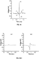
- An example of this class of signals is the heart beat in an ECG waveform as illustrated in Fig. 1A .
- the structure of a heart beat is defined by its P Q R S T components. The location, size, and shape of these components convey critical information about the physical operation of the heart.
- the waveform may be modeled as a sum of Lorentzian (also known as Cauchy distribution) pulses, each of which includes a symmetric and an asymmetric component:
- Lorentzian also known as Cauchy distribution
- the waveform is considered to be formed from K pulses, each one denoted by an index k, and each one of which is defined by a center position t k , a width or damping factor a k , an amplitude for a symmetric pulse component c k , and an amplitude for an asymmetric pulse component d k .
- the number of Lorentzian pulses used to model a signal will depend on the nature of the signal.
- the asymmetric amplitude d k can be set to zero, which reduces the number of parameters used to model the waveform. This is possible with the ECG waveforms, but the results in general are less accurate.
- Figure 1B illustrates five Lorentzian pulses of the form set forth in Equation 1 whose parameters were extracted from the original waveform of Figure 1A using the methods described below.
- the sum of the pulses in Figure 1B is shown in Figure 1C .
- Figure 1C is a good reproduction of the original signal of Figure 1A .
- the signal from Figure 1A is accurately parameterized by 20 parameters, four parameters (c, d, a, and t) for each of the five Lorentzian pulses of Figure 1B and Equation 1.
- a method is required to derive the desired parameters from the original time domain data, which is typically a series of discrete waveform samples taken during the acquisition of an analog electrical signal output from electrodes coupled to a subject.
- the sampling rate may vary, but may be about 120-360 Hz, producing about 100-500 time domain samples of the waveform over the approximately 0.75 to 1.5 second time period of interest containing the P, Q, R, S, and T waveform features. It will be appreciated that parameterizing the waveform to 20 parameter values instead of the 100-500 original waveform sample values can produce a compression of the data by a factor of 5-25.
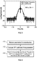
- FIG. 2 is a flow diagram of one method of signal analysis for deriving the VPW-FRI parameters in the frequency domain.
- the method starts at block 210, where a discrete Fourier transform (DFT) is performed on the original time domain samples.
- DFT discrete Fourier transform
- the method continues at block 212, where a set of MM positive frequency DFT coefficients are selected for further analysis to extract the above described pulse parameters.
- Figure 3 shows an ECG frequency spectrum produced from a DFT algorithm applied to a time domain ECG waveform sampled at 360 Hz.
- a spectrum typically includes a region of decaying oscillations around 0 Hz and a transition region where the spectral energy decreases with increasing frequency to 60 or 70 Hz.
- a noise floor of around -70 dB can also be seen in Figure 3 at frequencies above about 70 Hz.
- the details of the ECG waveform affect the frequencies and decay rate in the oscillating region, and the details of the shape of the transition region.
- the set of MM DFT coefficients selected for analysis is on the positive side of 0 Hz, and includes at least 2K+1 adjacent DFT coefficient values.
- positive frequency coefficients are selected because the set of coefficients cannot span across 0 Hz due to the methods used to perform the extraction as described further below.
- the selected set of coefficients should include the oscillating region from near 0 Hz and extend to cover at least some of the transition region as well.
- the pulse width and pulse location parameters a k and t k are calculated from at least some of the selected DFT coefficients.
- the method assumes that the DFT of block 210 was generated from a sampled time domain signal having the functional form of Equation 1.
- ⁇ j 2 ⁇ / ⁇ t k m f o r m ⁇ N 2 ... ,0, ... N 2 ⁇ 1
- an annihilating filter can be constructed having roots related to the parameters a k and t k .
- Techniques for solving this mathematical problem of deriving the parameters of a sampled (and possibly noisy) signal, where the signal is a sum of exponentially damped oscillations have been developed and are well known. For example, spectral analysis techniques such as the Prony algorithm are known that can construct the annihilating polynomial and find its roots. Other spectral analysis techniques can also be used to find the roots of the annihilation polynomial such as ESPRIT. Such techniques have been used for similar purposes such as the Dirac-FRI methods mentioned above.
- z k
- the symmetric and asymmetric amplitude parameters are extracted using a linear regression fit of DFT coefficients to be generated by Equation 2 to the DFT coefficients generated from the original time domain signal at block 210.
- a set of linear equations may be defined by matching a set of L values of X(m) from the input data with values expressed by the model in Equation 2. This set may be some or all of the MM previously selected coefficients, or any other selection of L values for m ⁇ 0.
- a minimum of K signal values and K equations ( L ⁇ K ) are needed to form a matrix equation which may be inverted (or least squares inverted) to obtain the values of b k .
- more signal values are generally used and the values of b k are determined by a least squares method.
- each b k is the symmetric amplitude c k of pulse k
- the imaginary part of each b k is the asymmetric amplitude d k of pulse k.
- the parameters are stored at block 218 for future signal reconstruction.
- the complete waveform can be compressed to four values for each pulse (plus potentially an additional DC shift parameter), which for a five pulse waveform is only twenty or twenty-one values, much less than the number of time domain (or frequency domain) values that would be stored as representative of the waveform if a conventional Nyquist rate sampling method were used.
- Figure 4 is a flow diagram of signal reconstruction from the stored parameters.
- the stored parameters a k , t k , c k , and d k are retrieved at block 410.
- DFT coefficients for positive m frequency indices are computed using Equation 2 and the retrieved parameters.
- Coefficients for negative m frequency indices may be computed by taking the complex conjugates of the positive m values produced by Equation 2.
- an inverse discrete Fourier transform is performed on the DFT coefficients, producing a set of time domain values that represent the original time domain signal.
- IDFT inverse discrete Fourier transform
- Equation 1 an alternative reconstruction method may be used in the time domain, where the parameters a k , t k , c k , and d k are plugged into Equation 1 to directly produce time domain data. Care should be taken in this case to use a shifted periodic version of Equation 1 if the original signal has any significant DC offset. This complication is not present if the frequency domain reconstruction of Figure 4 is utilized.
- Figures 5 and 6 show the results of the analysis of a real heart beat waveform obtained from the MIT/BIH data base.
- the original time domain data is shown in dashed line, and the reconstruction output from the above described method (at block 414 of Figure 4 for example) is shown in solid line.
- the DFT of the original signal (originally sampled at 360 Hz) is shown in dashed line, and the DFT coefficients produced by the method using Equation 2 at block 412 of Figure 4 are shown in solid line.
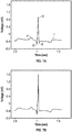
- Figure 8 illustrates the difference between the original waveform of Figure 7A and the reconstructed waveform of Figure 7B in the frequency domain.
- the dashed line illustrates the DFT of the original 360 Hz sampled waveform.
- the solid line illustrates the DFT coefficients produced by Equation 2 at, for example, block 412 of Figure 4 following extraction of the VPW-FRI parameters from the 60 Hz sample set.
- the deviation between the actual spectrum and the reconstructed spectrum becomes large above about 30 Hz (which corresponds to the sampling frequency of 60 Hz).
- the reconstruction overestimates the amplitudes. This produces the overshoot and missed S peak seen in the time domain data of Figures 7A and 7B .
- FIG. 9 a set of DFT coefficients modified from the original outputs of Equation 2 is illustrated.
- the solid line of Figure 9 is a graph of DFT coefficient output from Equation 2 for the region from 0 Hz up to about 30 Hz denoted by line 814.
- the DFT coefficients For the DFT coefficients from 30 Hz up to about 100 Hz (or beyond), denoted by line 1016, the DFT coefficients have an amplitude that is the DFT coefficients output from Equation 2 as modified according to Equation 9.
- the DFT now follows the parabolic shape defined between 15 Hz and 30 Hz all the way out to 100 Hz or more. In practice, the DFT coefficients past 60 to 80 Hz have little effect on the reconstruction.
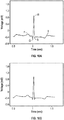
- Figure 10A shows the original time domain waveform sampled at 360 Hz, the same as is shown in Figure 7A .
- Figure 10B shows the time domain waveform produced by performing an IDFT on the solid line DFT of Figure 9 . With the correction from 30 Hz and upward, it can be seen in Figure 10B that the overshoot of the R peak is removed, and the S peak is now reproduced.
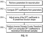
- Figure 11 is a flowchart illustrating this correction method. It generally follows the flow of Figure 4 , with the additional correction step described above.
- the stored parameters a k , t k , c k , and d k are retrieved at block 1110.
- DFT coefficients for positive m frequency indices are computed using Equation 2 and the retrieved parameters.
- Coefficients for negative m frequency indices may again be computed by taking the complex conjugates of the positive m values produced by Equation 2.
- some of the DFT coefficients are adjusted to fit a pre-defined function shape. For ECG waveforms, a parabolic functional shape has been found suitable. For other waveform sources, different functional shapes may be appropriate.
- IDFT inverse discrete Fourier transform
- the ⁇ and ⁇ parameters could be generated during the data analysis process described above with reference to Figure 2 .
- the parabolic curve fitting could be performed by generating the DFT coefficients from the extracted VPW-FRI parameters a, t, c, and d using Equation 2, generating a suitable ⁇ and ⁇ , and then storing these values along with the other VPW-FRI parameters. This eliminates the need to perform the parabolic curve fitting during reconstruction.
- Figure 12A illustrates a block diagram of one device configured to implement the VPW-FRI methods.
- the device may include a processor 1210.
- the processor 1210 may also be referred to as a central processing unit (CPU).
- Memory 1212 which may include both read-only memory (ROM) and random access memory (RAM), provides instructions and data to the processor 1210.
- a portion of the memory 1212 may also include non-volatile random access memory (NVRAM).
- the processor 1210 typically performs logical and arithmetic operations based on program instructions stored within the memory 1212.
- the instructions in the memory 1212 may be executable to implement the methods of the VPW-FRI model described herein.
- the instructions in the memory 1212 may be executable by the processor 1210 to implement the sequence of signal processing steps for the analysis and/or reconstruction of a waveform as shown in Figures 2 , 4 , and 11 .
- the processor 1210 may be configured to receive N samples (where N is a positive integer) of an input signal in the time domain from a local signal storage 1218 or a remote signal storage 1220. Further, the processor 1210 may transform the N samples utilizing a DFT algorithm to produce the transform coefficients X(m) in the frequency domain as described above. Alternatively, the signal storage may store DFT coefficients of original time domain signals, and these could be used as a starting point for the algorithm implemented by the processor 1210. A subset MM of the transform coefficients (whether received by or generated by the processor 1210), in particular a set of coefficients associated with positive frequencies, may be selected by the processor 1210. The subset MM of the transform coefficients may then be used by the processor to define the VPW-FRI parameters.
- the processor may also be configured to retrieve VPW-FRI parameters from the signal storage memory 1218 or 1220.
- the processor may then generate DFT coefficients using the methods described above, and perform an IDFT on the generated DFT coefficients to reconstruct a time domain waveform.
- An output device such display 1214 or a printer may be used to display either original or reconstructed time domain data.
- the signal storage memory 1218 and/or 1220 may comprise an ECG signal database.
- the processor may then use as input ECG signals, and store them as parameters computed utilizing the VPW-FRI algorithm. Storage of the ECG signals as such parameters may reduce the memory allocation necessary for storing such ECG signals.
- the system of Figure 12A may be employed, for example, at a hospital to efficiently store ECG signals as part of patient medical history records.
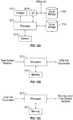
- FIGS 12B and 12C are block diagrams illustrating that different processors 1210 which may be geographically separated can separately perform the signal analysis and signal reconstruction.
- the processor 1210 is dedicated to performing the signal analysis portion of the process. This processor takes time domain samples and produces VPW-FRI parameters.
- the processor is dedicated to reconstruction. This processor takes VPW-FRI parameters as an input, and produces reconstructed time domain samples as an output.
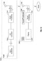
- FIG. 13 illustrates another system in which the above described methods can be implemented.
- a patch ECG monitor 1300 incorporates ECG electrodes 1312 and is mounted with adhesive for example on a subject as an ambulatory cardiac monitoring device.
- the signal from the electrodes is routed to an A/D converter 1314 which produces time domain samples of the signal.
- signal processing circuitry 1316 which may be configured to produce the VPW-FRI parameters of pulse width, time, and symmetric and asymmetric amplitude described above.
- These may be sent wirelessly via antenna 1318 to a mobile device 1340 such as a cell phone, tablet, or other portable electronic system, which receives the parameters via antenna 1342 and routes the parameters to signal processing circuitry 1344 in the mobile device 1340.
- the signal processing circuitry may also produce the ⁇ and ⁇ parameters and send them to the mobile device for curve fitting during reconstruction described above. It will be appreciated that the components of the patch 1300 need not be mounted together on the same physical substrate, but could be split up in a variety of ways.
- the signal processing circuitry 1344 in the mobile device 1340 may be configured to reconstruct the ECG waveforms using the VPW-FRI parameters and the ⁇ and ⁇ parameters that are computed on the mobile device 1340 or are received from the patch monitor 1300.
- the reconstructed signal may be displayed on a display 1346 and manipulated with a keypad/touchscreen 1348 on the mobile device.
- the mobile device may also be configured to transmit either the reconstructed waveform and/or the parameters to an external network such as the Internet for storage, review by a physician, etc.
- the on-body mounted system 1300 should use as little power as possible, it is advantageous to minimize the sampling rate of the A/D converter and also minimize the amount of data that must be transmitted from the on-body system 1300 to the mobile device 1340.
- the compression and accurate reconstruction provided by the methods described above can reduce the power consumed by the on-body system 1300.
- the hardware and data processing apparatus used to implement the various illustrative logics, logical blocks, modules and circuits described in connection with the aspects disclosed herein may be implemented or performed with a general purpose single- or multi-chip processor, a digital signal processor (DSP), an application specific integrated circuit (ASIC), a field programmable gate array (FPGA) or other programmable logic device, discrete gate or transistor logic, discrete hardware components, or any combination thereof designed to perform the functions described herein.
- a general purpose processor may be a microprocessor, or, any conventional processor, controller, microcontroller, or state machine.
- a processor may also be implemented as a combination of computing devices, e.g., a combination of a DSP and a microprocessor, a plurality of microprocessors, one or more microprocessors in conjunction with a DSP core, or any other such configuration.
- particular steps and methods may be performed by circuitry that is specific to a given function.
- the functions described may be implemented in hardware, digital electronic circuitry, computer software, firmware, including the structures disclosed in this specification and their structural equivalents thereof, or in any combination thereof. Implementations of the subject matter described in this specification also can be implemented as one or more computer programs, i.e., one or more modules of computer program instructions, encoded on a computer storage media for execution by, or to control the operation of, data processing apparatus.
- Computer-readable media includes both computer storage media and communication media including any medium that can be enabled to transfer a computer program from one place to another.
- a storage media may be any available media that may be accessed by a computer.
- such computer-readable media may include RAM, ROM, EEPROM, CD-ROM or other optical disk storage, magnetic disk storage or other magnetic storage devices, or any other medium that may be used to store desired program code in the form of instructions or data structures and that may be accessed by a computer.
- Disk and disc includes compact disc (CD), laser disc, optical disc, digital versatile disc (DVD), floppy disk, and blu-ray disc where disks usually reproduce data magnetically, while discs reproduce data optically with lasers. Combinations of the above should also be included within the scope of computer-readable media. Additionally, the operations of a method or algorithm may reside as one or any combination or set of codes and instructions on a machine readable medium and computer-readable medium, which may be incorporated into a computer program product.
Landscapes
- Health & Medical Sciences (AREA)
- Physics & Mathematics (AREA)
- Engineering & Computer Science (AREA)
- Life Sciences & Earth Sciences (AREA)
- Mathematical Physics (AREA)
- General Physics & Mathematics (AREA)
- Mathematical Optimization (AREA)
- Mathematical Analysis (AREA)
- Biomedical Technology (AREA)
- Veterinary Medicine (AREA)
- Data Mining & Analysis (AREA)
- Public Health (AREA)
- General Health & Medical Sciences (AREA)
- Animal Behavior & Ethology (AREA)
- Theoretical Computer Science (AREA)
- Pure & Applied Mathematics (AREA)
- Surgery (AREA)
- Molecular Biology (AREA)
- Computational Mathematics (AREA)
- Medical Informatics (AREA)
- Heart & Thoracic Surgery (AREA)
- Pathology (AREA)
- Biophysics (AREA)
- Cardiology (AREA)
- Physiology (AREA)
- Discrete Mathematics (AREA)
- General Engineering & Computer Science (AREA)
- Software Systems (AREA)
- Databases & Information Systems (AREA)
- Algebra (AREA)
- Psychiatry (AREA)
- Computer Vision & Pattern Recognition (AREA)
- Artificial Intelligence (AREA)
- Computer Networks & Wireless Communication (AREA)
- Signal Processing (AREA)
- Measurement And Recording Of Electrical Phenomena And Electrical Characteristics Of The Living Body (AREA)
- Complex Calculations (AREA)
- Measurement Of Resistance Or Impedance (AREA)
Description
- This disclosure relates to systems and methods for applying a predefined functional shape to coefficients of a discrete Fourier transform of a waveform.
- Signal parameterization is widely used in signal processing, storage, transmission, and analysis. Perhaps the most common is the use of Nyquist rate sampling, where a continuous time domain signal is represented by a set of sampled signal values at discrete times. As long as the original continuous signal is band limited to at most half the sampling rate, the set of samples can be used to reconstruct the complete signal by using, for example, a sinc interpolation algorithm, see also Abdelaziz Ouamri, Amine N.-Ali: ECG compression method using Lorentzian functions model; Digital Signal Processing, vol 17, no. 1,2, December 2006, pages 319-326. In this common example, the signal is represented by a set of discrete parameters, the sample values, which can be stored, transmitted, and used at any time to completely reconstruct the original signal.
- More recently, some non-bandlimited signals of practical interest have been parameterized in other ways. Although these signals may contain frequency components that are arbitrarily large, they are modeled by characteristics that limit the "rate-of-innovation" per unit time so that the signal can be parameterized with a finite set of values from which the original signal can be reconstructed. The problem to be solved then is how to derive a suitable set of parameter values from the original signal and how to reverse the process to reconstruct the complete signal using only the derived parameters. The prior art of Finite Rate of Innovation (FRI) based signal analysis is one such method of analyzing signals and is described in the following references: [1] M. Vetterli, P. Marziliano, T. Blu, "Sampling Signals with Finite Rate of Innovation", IEEE Transactions on Signal Procesing, vol. 50, no. 6, pp. 1417-1428, June 2002; [2] T. Blu, P.L. Dragotti, M. Vetterli, P. Marziliano, and L Coulot, "Sparse Sampling of Signal Innovations: Theory, Algorithms, and Performance Bounds", IEEE Signal Processing Magazine, vol. 25, no.2, pp. 31-40, March 2008; [3] Y. Hao, P. Marziliano, M. Vetterli, T. Blu, "Compression of ECG as a Signal with Finite Rate of Innovation", Proc. of the 2005 IEEE Engineering in Medicine and Biology 27th Annual Conference, Shanghai, China, September 1-4, 2005, pp. 7564 - 7567; [4] Marziliano, M. Vetterli and T. Blu, "Sampling and Exact Reconstruction of Bandlimited Signals With Additive Shot Noise," IEEE Transactions on Information Theory, vol. 52, No. 5, pp. 2230-2233, May 2006. In this method, waveforms or derivatives of waveforms are analyzed to identify the locations and amplitudes of Dirac functions (essentially infinitely narrow pulses) which are used to define signal features or markers for the boundaries of signal segments within the pseudo-periods. The signals or signal segments may then be reconstructed using the appropriate wave shapes or splines. These models (which may be referred to as Dirac-FRI models) described in the prior art are limited to two parameters for pulse descriptions, an amplitude and a position within a period (for pseudo-periodic signals), and they are restricted to a single pulse shape for reconstruction. Thus these models are limited in their ability to parameterize signals containing pulses of varying widths.
- The systems, methods, and devices of the invention each have several aspects, no single one of which is solely responsible for its desirable attributes. Without limiting the scope of this invention as expressed by the claims which follow, some features will now be discussed briefly. After considering this discussion, and particularly after reading the section entitled "Detailed Description" one will understand how the features of this invention provide advantages that include models for defining and parameterizing signals or system responses containing pulses of varying width. The parameters may define the signal and therefore can be used as a compressed version of the original signal. Storage of the parameters as a compressed version of the signal requires less storage space, making storage of signals more memory efficient.
- In one implementation, a computer implemented method of reconstructing a time domain waveform from a compressed original time domain waveform comprises receiving, by a processor, parameters defining a compressed form of the original time domain waveform, generating, with the processor, discrete Fourier transform (DFT) coefficients from the parameters, adjusting, with the processor, the amplitudes of at least some of the generated DFT coefficients to more closely fit the amplitudes of at least some of the generated DFT coefficients to a predefined functional shape, performing, with the processor, an inverse discrete Fourier transform (IDFT) on a set of DFT coefficients including the adjusted DFT coefficients to produce a reconstructed time domain waveform. In some implementations, the predefined functional shape is parabolic on a logarithmic scale. In some implementations, the waveform is based, at least on part, on an electro-cardiogram (ECG). In some implementations, the parameters are derived from time domain samples of an original signal, and the time domains samples may be spaced at less than 120 Hz.
- In another aspect, an processing apparatus comprises a memory having stored therein parameters defining a compressed form of an original time domain waveform, a processor configured to retrieve parameters, generate discrete Fourier transform (DFT) coefficients from the parameters, and adjust the amplitudes of at least some of the generated DFT coefficients to more closely fit the amplitudes of the at least some of the generated DFT coefficients to a predefined functional shape. The processor is also configured toperform an inverse discrete Fourier transform (IDFT) on a set of DFT coefficients including the adjusted DFT coefficients to produce a reconstructed time domain waveform.
- In another aspect, a non-transitory, computer readable medium is disclosed, which comprises instructions that when executed cause a processor to perform a method comprising receivingving, in the processor, parameters defining a compressed form of an original time domain waveform, generating, with the processor, discrete Fourier transform (DFT) coefficients from the parameters, adjusting, with the processor, the amplitudes of at least some of the generated DFT coefficients to more closely fit the amplitudes of at least some of the generated DFT coefficients to a predefined functional shape, performing, with the processor, an inverse discrete Fourier transform (IDFT) on a set of DFT coefficients including the adjusted DFT coefficients to produce a reconstructed time domain waveform.
-
-
FIGs. 1A-1C illustrate reconstruction of an ECG waveform with a sum of Lorentzian pulses. -
FIG. 2 is a flow chart of a method of parameterizing waveform containing variable width pulses. -
FIG. 3 is a graph of the spectrum of an ECG waveform. -
FIG. 4 is a flowchart of a method of signal reconstruction using the parameters generated with the method ofFigure 2 . -
FIG. 5 is a graph comparing an original time domain signal with a reconstruction of the signal using VPW-FRI parameters. -
FIG. 6 is a graph comparing the time domain waveforms ofFigure 5 in the frequency domain. -
FIGs. 7A and 7B illustrate an original time domain ECG waveform and a reconstruction of the waveform using downsampled data. -
FIG. 8 is a graph comparing the time domain waveforms ofFigures 7A and 7B in the frequency domain. -
FIG. 9 is a graph comparing the frequency domain waveform ofFigure 7A with an adjusted frequency domain waveform used for reconstruction. -
FIGs. 10A and 10B illustrate an original time domain ECG waveform and a reconstruction of the waveform using the adjusted frequency domain waveform ofFigure 9 . -
FIG. 11 is a flow chart of a method of signal reconstruction including DFT coefficient adjustment. -
FIGs. 12A-12C illustrates embodiments of systems utilizing signal parameterization of the present disclosure. -
FIG. 13 illustrates an embodiment of a system utilizing signal parameterization of the present disclosure. - Various aspects of the novel systems, apparatuses, and methods are described more fully hereinafter with reference to the accompanying drawings. The teachings may be embodied in many different forms and should not be construed as limited to any specific structure or function presented throughout this disclosure. Rather, these aspects are provided so that this disclosure will be thorough and complete, and will fully convey the scope of the disclosure to those skilled in the art. Based on the teachings herein one skilled in the art should appreciate that the scope of the disclosure is intended to cover any aspect of the novel systems, apparatuses, and methods disclosed herein, whether implemented independently of or combined with any other aspect of the invention. For example, an apparatus may be implemented or a method may be practiced using any number of the aspects set forth herein. In addition, the scope of the invention is intended to cover such an apparatus or method which is practiced using other structure, functionality, or structure and functionality in addition to or other than the various aspects of the invention set forth herein. It should be understood that any aspect disclosed herein may be embodied by one or more elements of a claim.
- Although particular aspects are described herein, many variations and permutations of these aspects fall within the scope of the disclosure. Although some benefits and advantages of the preferred aspects are mentioned, the scope of the disclosure is not intended to be limited to particular benefits, uses, or objectives. Rather, aspects of the disclosure are intended to be broadly applicable to different systems, some of which are illustrated by way of example in the figures and in the following description of the preferred aspects. The detailed description and drawings are merely illustrative of the disclosure rather than limiting, the scope of the disclosure being defined by the appended claims and equivalents thereof.
- The methods of the present disclosure may be applicable to a variety of systems. For example, the present disclosure may be particularly applicable to signal storage databases such as electro-cardiogram (ECG) databases. In one aspect, the methods herein may be used to parameterize ECG signals and then store those parameters in an ECG database. This may greatly reduce the cost and resources required for storing ECG signals as the memory allocation required to store the data is greatly reduced. Such ECG signal databases provide information used for evaluation and treatment of patients. Further, hospitals may require such ECG databases as part of storage of patient medical records. Thus, the systems and methods described herein may prove valuable to the medical field.
- Many of the methods described herein overcome difficulties of the prior art by introducing parameters in the model which define the widths and asymmetries of the pulse shapes of the model and extends the mathematics and methodology of FRI analysis. Additionally, the disclosure defines the means for performing the analysis to estimate these parameters from the data. It generalizes the model of FRI to a four-parameter pulse model which can represent waveforms as the sum of overlapping pulses (defined by complex poles in the model), each of which is characterized by a position, symmetric component amplitude, asymmetric component amplitude, and width. The added degrees of freedom provided by this generalization greatly extend the range and class of signals that can be modeled and it permits the representation of overlapping of pulses rather than concatenations of waveform segments.
- Signals that approximate the parameterization model described herein may be referred to as Variable Pulse-Width Finite Rate of Information (i.e. the VPW-FRI) signals. An example of this class of signals is the heart beat in an ECG waveform as illustrated in
Fig. 1A . As seen by this figure, the structure of a heart beat is defined by its P Q R S T components. The location, size, and shape of these components convey critical information about the physical operation of the heart. In the VPW-FRI model, the waveform may be modeled as a sum of Lorentzian (also known as Cauchy distribution) pulses, each of which includes a symmetric and an asymmetric component:
- In this model, the waveform is considered to be formed from K pulses, each one denoted by an index k, and each one of which is defined by a center position tk, a width or damping factor ak, an amplitude for a symmetric pulse component ck, and an amplitude for an asymmetric pulse component dk. The number of Lorentzian pulses used to model a signal will depend on the nature of the signal. For an ECG waveform, using a K of five has been found generally suitable to reproduce the P, Q, R, S, and T features that are of clinical significance, although more robust results have been found in some cases if a six or seven pulse model is used, especially when the ECG waveforms being modeled have a relatively large amount of noise.
- For some signal waveforms, the asymmetric amplitude dk can be set to zero, which reduces the number of parameters used to model the waveform. This is possible with the ECG waveforms, but the results in general are less accurate.
-
Figure 1B illustrates five Lorentzian pulses of the form set forth inEquation 1 whose parameters were extracted from the original waveform ofFigure 1A using the methods described below. The sum of the pulses inFigure 1B is shown inFigure 1C . It can be seen thatFigure 1C is a good reproduction of the original signal ofFigure 1A . In this way, the signal fromFigure 1A is accurately parameterized by 20 parameters, four parameters (c, d, a, and t) for each of the five Lorentzian pulses ofFigure 1B andEquation 1. - As with other parameterization techniques, a method is required to derive the desired parameters from the original time domain data, which is typically a series of discrete waveform samples taken during the acquisition of an analog electrical signal output from electrodes coupled to a subject. The sampling rate may vary, but may be about 120-360 Hz, producing about 100-500 time domain samples of the waveform over the approximately 0.75 to 1.5 second time period of interest containing the P, Q, R, S, and T waveform features. It will be appreciated that parameterizing the waveform to 20 parameter values instead of the 100-500 original waveform sample values can produce a compression of the data by a factor of 5-25.
- Although it may be possible to perform a derivation of the pulse parameters in the time domain (by, for example, using a regression analysis to find a, t, c, and d values for each of the five pulses that minimizes the differences between the values produced by
Equation 1 at the sample times and the actual sample values), significant computational and accuracy advantages arise from performing the parameter derivation in the frequency domain. -
Figure 2 is a flow diagram of one method of signal analysis for deriving the VPW-FRI parameters in the frequency domain. In this implementation, the method starts atblock 210, where a discrete Fourier transform (DFT) is performed on the original time domain samples. The method continues atblock 212, where a set of MM positive frequency DFT coefficients are selected for further analysis to extract the above described pulse parameters. These steps are also illustrated graphically inFigure 3 , which shows an ECG frequency spectrum produced from a DFT algorithm applied to a time domain ECG waveform sampled at 360 Hz. As can be seen inFigure 3 , such a spectrum typically includes a region of decaying oscillations around 0 Hz and a transition region where the spectral energy decreases with increasing frequency to 60 or 70 Hz. A noise floor of around -70 dB can also be seen inFigure 3 at frequencies above about 70 Hz. The details of the ECG waveform affect the frequencies and decay rate in the oscillating region, and the details of the shape of the transition region. - The set of MM DFT coefficients selected for analysis is on the positive side of 0 Hz, and includes at least 2K+1 adjacent DFT coefficient values. For the extraction method described in more detail below, positive frequency coefficients are selected because the set of coefficients cannot span across 0 Hz due to the methods used to perform the extraction as described further below. The extraction method described below also requires at least 2K+1 values as inputs, although stability and accuracy of results in the presence of noise is improved if more than this number are utilized. If K=5 (e.g. 5 pulse model) for an ECG waveform, it has been found useful for the number MM to be at least 25 or 30 DFT coefficients rather than the minimum of 11. The selected set of coefficients should include the oscillating region from near 0 Hz and extend to cover at least some of the transition region as well.
- Referring back to
Figure 2 , atblock 214, the pulse width and pulse location parameters ak and tk are calculated from at least some of the selected DFT coefficients. To extract the damping factor (also referred to as the pulse width factor) ak and the time tk of each pulse, the method assumes that the DFT ofblock 210 was generated from a sampled time domain signal having the functional form ofEquation 1. The DFT coefficients of a sampled sum of such Lorentzian pulses will follow the form of a sum of decaying sinusoids as shown in Equation 2:
- where bk = ck - jdk for positive m
- bk = ck + jdk for negative m
- τ = N/Fs , where Fs is the time domain sampling frequency and N is the number of time domain samples taken during the period of interest
- If the DFT of the original signal is assumed to be of the functional form of
Equation 2, an annihilating filter can be constructed having roots related to the parameters ak and tk. Techniques for solving this mathematical problem of deriving the parameters of a sampled (and possibly noisy) signal, where the signal is a sum of exponentially damped oscillations, have been developed and are well known. For example, spectral analysis techniques such as the Prony algorithm are known that can construct the annihilating polynomial and find its roots. Other spectral analysis techniques can also be used to find the roots of the annihilation polynomial such as ESPRIT. Such techniques have been used for similar purposes such as the Dirac-FRI methods mentioned above. Past attempts to use such methods, however, generally used DFT coefficients that include both positive and negative frequencies. When the pulses are assumed to have variable width, however, this presents a discontinuity, as can be seen fromEquation 2, and the Prony algorithm, for example, does not model curves with exponential weights that change within the domain of analysis. One method of solving this problem is by recognizing that the spectrum of the time domain signal is conjugate symmetric, and it is not necessary that the coefficients used in thealgorithm span 0 Hz. One can use only positive or only negative components of the spectrum (plus 0 Hz if desired) to satisfy the conditions of the Prony method. The complex roots of the annihilator polynomial in the spectral analysis will then provide the information to determine the damping factors in the model in addition to the pulse times. An additional advantage is gained by the recognition that frequency components supplied to the Prony method do not have to start at m=0. Since data obtained from real applications is often corrupted by DC offsets, it can be advantageous to avoid the m=0 term and, in some cases, the m=1 term in the analysis. - When one of the above described spectral analysis techniques is applied in this manner, this polynomial will have K roots which are (in polar form):

- It can be seen that the magnitude and phase of the roots are as follows:

- From these roots, the pulse locations tk can be computed:

- The damping factors, ak , are related to the magnitudes of the roots by the relation:

- After finding the damping factors and pulse times, at
block 216 ofFigure 2 the symmetric and asymmetric amplitude parameters are extracted using a linear regression fit of DFT coefficients to be generated byEquation 2 to the DFT coefficients generated from the original time domain signal atblock 210. - To accomplish this, a set of linear equations may be defined by matching a set of L values of X(m) from the input data with values expressed by the model in
Equation 2. This set may be some or all of the MM previously selected coefficients, or any other selection of L values for m ≥ 0. A minimum of K signal values and K equations (L ≥ K) are needed to form a matrix equation which may be inverted (or least squares inverted) to obtain the values of bk . In practice, more signal values are generally used and the values of bk are determined by a least squares method. - The above set of linear equations can be described as follows:


- Defining:


- The solution for c can be expressed as:


inv(G) is the least squares (Moore-Penrose) pseudo-inverse of the matrix G. - When the components of the column vector [b] are determined with this method, the real part of each bk is the symmetric amplitude ck of pulse k, and the imaginary part of each bk is the asymmetric amplitude dk of pulse k.
- After all the parameters ak, tk, ck, and dk are calculated, the parameters are stored at
block 218 for future signal reconstruction. When this model is applied, the complete waveform can be compressed to four values for each pulse (plus potentially an additional DC shift parameter), which for a five pulse waveform is only twenty or twenty-one values, much less than the number of time domain (or frequency domain) values that would be stored as representative of the waveform if a conventional Nyquist rate sampling method were used. -
Figure 4 is a flow diagram of signal reconstruction from the stored parameters. In this implementation, the stored parameters ak, tk, ck, and dk are retrieved atblock 410. From the stored parameters, atblock 412 DFT coefficients for positive m frequency indices are computed usingEquation 2 and the retrieved parameters. Coefficients for negative m frequency indices may be computed by taking the complex conjugates of the positive m values produced byEquation 2. Atblock 414, an inverse discrete Fourier transform (IDFT) is performed on the DFT coefficients, producing a set of time domain values that represent the original time domain signal. It will be appreciated that an alternative reconstruction method may be used in the time domain, where the parameters ak, tk, ck, and dk are plugged intoEquation 1 to directly produce time domain data. Care should be taken in this case to use a shifted periodic version ofEquation 1 if the original signal has any significant DC offset. This complication is not present if the frequency domain reconstruction ofFigure 4 is utilized. - To illustrate the utility of this approach, the VPW-FRI model and the analysis method defined by this disclosure,
Figures 5 and 6 show the results of the analysis of a real heart beat waveform obtained from the MIT/BIH data base. InFigure 5 , the original time domain data is shown in dashed line, and the reconstruction output from the above described method (atblock 414 ofFigure 4 for example) is shown in solid line. InFigure 6 , the DFT of the original signal (originally sampled at 360 Hz) is shown in dashed line, and the DFT coefficients produced by themethod using Equation 2 atblock 412 ofFigure 4 are shown in solid line. - The above method of signal processing works very well for ECG waveforms that are sampled at relatively high rates such as 120 Hz or more. In practice, however, stored time domain samples often have lower frequency, sometimes being downsampled to 60 Hz, for example. When lower frequency sampled data is used, the VPW-FRI algorithm may not accurately reproduce all of the important features of the waveform. This is illustrated in
Figures 7A and 7B , which illustrate an original 360 Hz sampled ECG waveform and a VPW-FRI reconstruction of the waveform ofFigure 7A when the input data is not the 360 Hz original data, but is a decimated data set with a 60 Hz sample frequency instead where only one original sample in six is used for analysis and reconstruction. As can be seen inFigure 7B , the R peak has a strong overshoot in amplitude, and the small S peak inFigure 7A is essentially absent inFigure 7B . -
Figure 8 illustrates the difference between the original waveform ofFigure 7A and the reconstructed waveform ofFigure 7B in the frequency domain. InFigure 8 , the dashed line illustrates the DFT of the original 360 Hz sampled waveform. The solid line illustrates the DFT coefficients produced byEquation 2 at, for example, block 412 ofFigure 4 following extraction of the VPW-FRI parameters from the 60 Hz sample set. The deviation between the actual spectrum and the reconstructed spectrum becomes large above about 30 Hz (which corresponds to the sampling frequency of 60 Hz). In general, for frequencies from 30 to 100 Hz, the reconstruction overestimates the amplitudes. This produces the overshoot and missed S peak seen in the time domain data ofFigures 7A and 7B . - To improve signal reconstruction with downsampled original data, it has been observed that on a log scale, the amplitudes of the DFT coefficients of ECG waveforms tend to follow a parabolic functional form (on the log scale) in the transition region above about 10-15 Hz until the signal becomes basically noise at 60-100 Hz. This region is denoted 812 in
Figure 8 . Although different ECG waveforms may have wider or narrower parabolic shapes in this area and may be shifted up or down, ECG waveforms in general exhibit this parabolic form. - This observation can be taken advantage of by adjusting the magnitudes of the DFT coefficients output by
Equation 2 for m indices corresponding to frequencies higher than the input data sample frequency so that they follow the generally observed parabolic shape. To find the appropriate second order polynomial to use for the adjustment, the log of the reconstructed DFT data in the transition region corresponding to about 15 Hz to the input sample frequency is fit to a parameterized parabola of the form αm2 + β. This region extends from aboutline 814 toline 816 illustrated inFigure 8 . This is a region of the spectrum where the original DFT coefficients output fromEquation 2 in the reconstruction process follow the DFT of the actual data well. Because the parabola is centered at 0 Hz, there is no need for a linear term, and the coefficient α will be negative, since the parabola opens downward. The parameters α and β may be determined by finding α and β values that minimize the difference between the DFT coefficient amplitudes produced byEquation 2 and the DFT coefficient amplitudes produced by the formula logX[m] = αm2 + β as shown in Equation 8, where X[m] are the DFT magnitudes produced byEquation 2 in the region betweenline Figure 8 :
- Once the parameters α and β are determined, the magnitudes of the DFT coefficients produced by
Equation 2 can be adjusted (without changing the phase) in the region above the sample frequency where the original DFT coefficients do not reproduce the spectrum well. Thus, for DFT coefficients corresponding to frequencies above the input sample frequency, the DFT coefficients can be modified in accordance with Equation 9:
- The result of this procedure is illustrated graphically in
Figures 9 and10 . InFigure 9 , a set of DFT coefficients modified from the original outputs ofEquation 2 is illustrated. The solid line ofFigure 9 is a graph of DFT coefficient output fromEquation 2 for the region from 0 Hz up to about 30 Hz denoted byline 814. For the DFT coefficients from 30 Hz up to about 100 Hz (or beyond), denoted by line 1016, the DFT coefficients have an amplitude that is the DFT coefficients output fromEquation 2 as modified according to Equation 9. The DFT now follows the parabolic shape defined between 15 Hz and 30 Hz all the way out to 100 Hz or more. In practice, the DFT coefficients past 60 to 80 Hz have little effect on the reconstruction.Figure 10A shows the original time domain waveform sampled at 360 Hz, the same as is shown inFigure 7A .Figure 10B shows the time domain waveform produced by performing an IDFT on the solid line DFT ofFigure 9 . With the correction from 30 Hz and upward, it can be seen inFigure 10B that the overshoot of the R peak is removed, and the S peak is now reproduced. -
Figure 11 is a flowchart illustrating this correction method. It generally follows the flow ofFigure 4 , with the additional correction step described above. As also described above with reference toFigure 4 , the stored parameters ak, tk, ck, and dk are retrieved at block 1110. From the stored parameters, at block 1112 DFT coefficients for positive m frequency indices are computed usingEquation 2 and the retrieved parameters. Coefficients for negative m frequency indices may again be computed by taking the complex conjugates of the positive m values produced byEquation 2. At block 1114, some of the DFT coefficients are adjusted to fit a pre-defined function shape. For ECG waveforms, a parabolic functional shape has been found suitable. For other waveform sources, different functional shapes may be appropriate. At block 1116, an inverse discrete Fourier transform (IDFT) is performed on the DFT coefficients, producing a set of time domain values that represent the original time domain signal. - It will be appreciated that the α and β parameters could be generated during the data analysis process described above with reference to
Figure 2 . In this implementation, the parabolic curve fitting could be performed by generating the DFT coefficients from the extracted VPW-FRI parameters a, t, c, andd using Equation 2, generating a suitable α and β, and then storing these values along with the other VPW-FRI parameters. This eliminates the need to perform the parabolic curve fitting during reconstruction. - The methods described above can be implemented in a wide variety of systems.
Figure 12A illustrates a block diagram of one device configured to implement the VPW-FRI methods. The device may include aprocessor 1210. Theprocessor 1210 may also be referred to as a central processing unit (CPU).Memory 1212, which may include both read-only memory (ROM) and random access memory (RAM), provides instructions and data to theprocessor 1210. A portion of thememory 1212 may also include non-volatile random access memory (NVRAM). Theprocessor 1210 typically performs logical and arithmetic operations based on program instructions stored within thememory 1212. The instructions in thememory 1212 may be executable to implement the methods of the VPW-FRI model described herein. For example, the instructions in thememory 1212 may be executable by theprocessor 1210 to implement the sequence of signal processing steps for the analysis and/or reconstruction of a waveform as shown inFigures 2 ,4 , and11 . - The
processor 1210 may be configured to receive N samples (where N is a positive integer) of an input signal in the time domain from alocal signal storage 1218 or a remote signal storage 1220. Further, theprocessor 1210 may transform the N samples utilizing a DFT algorithm to produce the transform coefficients X(m) in the frequency domain as described above. Alternatively, the signal storage may store DFT coefficients of original time domain signals, and these could be used as a starting point for the algorithm implemented by theprocessor 1210. A subset MM of the transform coefficients (whether received by or generated by the processor 1210), in particular a set of coefficients associated with positive frequencies, may be selected by theprocessor 1210. The subset MM of the transform coefficients may then be used by the processor to define the VPW-FRI parameters. These parameters may then be stored as compressed versions of the original data insignal storage 1218 or 1220. The original data can then be discarded or stored elsewhere. The processor may also be configured to retrieve VPW-FRI parameters from thesignal storage memory 1218 or 1220. The processor may then generate DFT coefficients using the methods described above, and perform an IDFT on the generated DFT coefficients to reconstruct a time domain waveform. An output devicesuch display 1214 or a printer may be used to display either original or reconstructed time domain data. - The
signal storage memory 1218 and/or 1220 may comprise an ECG signal database. The processor may then use as input ECG signals, and store them as parameters computed utilizing the VPW-FRI algorithm. Storage of the ECG signals as such parameters may reduce the memory allocation necessary for storing such ECG signals. The system ofFigure 12A may be employed, for example, at a hospital to efficiently store ECG signals as part of patient medical history records. - Although a number of separate components are illustrated in
Figure 12A , those of skill in the art will recognize that one or more of the components may be combined or commonly implemented. Further, each of the components illustrated inFigure 12A may be implemented using a plurality of separate elements. -
Figures 12B and 12C are block diagrams illustrating thatdifferent processors 1210 which may be geographically separated can separately perform the signal analysis and signal reconstruction. InFigure 12B , theprocessor 1210 is dedicated to performing the signal analysis portion of the process. This processor takes time domain samples and produces VPW-FRI parameters. InFigure 12C , the processor is dedicated to reconstruction. This processor takes VPW-FRI parameters as an input, and produces reconstructed time domain samples as an output. -
Figure 13 illustrates another system in which the above described methods can be implemented. In this system, apatch ECG monitor 1300 incorporatesECG electrodes 1312 and is mounted with adhesive for example on a subject as an ambulatory cardiac monitoring device. The signal from the electrodes is routed to an A/D converter 1314 which produces time domain samples of the signal. These samples are sent to signalprocessing circuitry 1316 which may be configured to produce the VPW-FRI parameters of pulse width, time, and symmetric and asymmetric amplitude described above. These may be sent wirelessly viaantenna 1318 to amobile device 1340 such as a cell phone, tablet, or other portable electronic system, which receives the parameters viaantenna 1342 and routes the parameters to signalprocessing circuitry 1344 in themobile device 1340. As noted above, the signal processing circuitry may also produce the α and β parameters and send them to the mobile device for curve fitting during reconstruction described above. It will be appreciated that the components of thepatch 1300 need not be mounted together on the same physical substrate, but could be split up in a variety of ways. - The
signal processing circuitry 1344 in themobile device 1340 may be configured to reconstruct the ECG waveforms using the VPW-FRI parameters and the α and β parameters that are computed on themobile device 1340 or are received from thepatch monitor 1300. The reconstructed signal may be displayed on adisplay 1346 and manipulated with a keypad/touchscreen 1348 on the mobile device. The mobile device may also be configured to transmit either the reconstructed waveform and/or the parameters to an external network such as the Internet for storage, review by a physician, etc. - Because the on-body mounted
system 1300 should use as little power as possible, it is advantageous to minimize the sampling rate of the A/D converter and also minimize the amount of data that must be transmitted from the on-body system 1300 to themobile device 1340. The compression and accurate reconstruction provided by the methods described above can reduce the power consumed by the on-body system 1300. - The various illustrative logic, logical blocks, modules, and algorithm steps described in connection with the implementations disclosed herein may be implemented as electronic hardware, computer software, or combinations of both. The interchangeability of hardware and software has been described generally, in terms of functionality, and illustrated in the various illustrative components, blocks, modules, circuits and steps described above. Whether such functionality is implemented in hardware or software depends upon the particular application and design constraints imposed on the overall system.
- The hardware and data processing apparatus used to implement the various illustrative logics, logical blocks, modules and circuits described in connection with the aspects disclosed herein may be implemented or performed with a general purpose single- or multi-chip processor, a digital signal processor (DSP), an application specific integrated circuit (ASIC), a field programmable gate array (FPGA) or other programmable logic device, discrete gate or transistor logic, discrete hardware components, or any combination thereof designed to perform the functions described herein. A general purpose processor may be a microprocessor, or, any conventional processor, controller, microcontroller, or state machine. A processor may also be implemented as a combination of computing devices, e.g., a combination of a DSP and a microprocessor, a plurality of microprocessors, one or more microprocessors in conjunction with a DSP core, or any other such configuration. In some implementations, particular steps and methods may be performed by circuitry that is specific to a given function.
- In one or more aspects, the functions described may be implemented in hardware, digital electronic circuitry, computer software, firmware, including the structures disclosed in this specification and their structural equivalents thereof, or in any combination thereof. Implementations of the subject matter described in this specification also can be implemented as one or more computer programs, i.e., one or more modules of computer program instructions, encoded on a computer storage media for execution by, or to control the operation of, data processing apparatus.
- If implemented in software, the functions may be stored on or transmitted over as one or more instructions or code on a computer-readable medium. The steps of a method or algorithm disclosed herein may be implemented in a processor-executable software module which may reside on a computer-readable medium. Computer-readable media includes both computer storage media and communication media including any medium that can be enabled to transfer a computer program from one place to another. A storage media may be any available media that may be accessed by a computer. By way of example, and not limitation, such computer-readable media may include RAM, ROM, EEPROM, CD-ROM or other optical disk storage, magnetic disk storage or other magnetic storage devices, or any other medium that may be used to store desired program code in the form of instructions or data structures and that may be accessed by a computer. Also, any connection can be properly termed a computer-readable medium. Disk and disc, as used herein, includes compact disc (CD), laser disc, optical disc, digital versatile disc (DVD), floppy disk, and blu-ray disc where disks usually reproduce data magnetically, while discs reproduce data optically with lasers. Combinations of the above should also be included within the scope of computer-readable media. Additionally, the operations of a method or algorithm may reside as one or any combination or set of codes and instructions on a machine readable medium and computer-readable medium, which may be incorporated into a computer program product.
- Various modifications to the implementations described in this disclosure may be readily apparent to those skilled in the art, and the generic principles defined herein may be applied to other implementations without departing from the spirit or scope of this disclosure. Thus, the disclosure is not intended to be limited to the implementations shown herein, but is to be accorded the widest scope consistent with the claims, the principles and the novel features disclosed herein. The word "exemplary" is used exclusively herein to mean "serving as an example, instance, or illustration." Any implementation described herein as "exemplary" is not necessarily to be construed as preferred or advantageous over other implementations.
- Certain features that are described in this specification in the context of separate implementations also can be implemented in combination in a single implementation. Conversely, various features that are described in the context of a single implementation also can be implemented in multiple implementations separately or in any suitable subcombination. Moreover, although features may be described above as acting in certain combinations and even initially claimed as such, one or more features from a claimed combination can in some cases be excised from the combination, and the claimed combination may be directed to a subcombination or variation of a subcombination.
- Similarly, while operations are depicted in the drawings in a particular order, this should not be understood as requiring that such operations be performed in the particular order shown or in sequential order, or that all illustrated operations be performed, to achieve desirable results. Further, the drawings may schematically depict one more example processes in the form of a flow diagram. However, other operations that are not depicted can be incorporated in the example processes that are schematically illustrated. For example, one or more additional operations can be performed before, after, simultaneously, or between any of the illustrated operations. In certain circumstances, multitasking and parallel processing may be advantageous. Moreover, the separation of various system components in the implementations described above should not be understood as requiring such separation in all implementations, and it should be understood that the described program components and systems can generally be integrated together in a single software product or packaged into multiple software products. Additionally, other implementations are within the scope of the following claims. In some cases, the actions recited in the claims can be performed in a different order and still achieve desirable results.
Claims (15)
- A computer implemented method of reconstructing a time domain waveform comprising:receiving (910), in a processor, parameters defining a compressed form of the original time domain waveform modeled as a sum of Lorentzian pulses;generating (912), with the processor, discrete Fourier transform, DFT, coefficients from the parameters;adjusting (914), with the processor, the amplitudes of at least some of the generated DFT coefficients to more closely fit to a predefined functional shape, wherein the at least some of the generated DFT coefficients correspond to frequencies higher than a sampling frequency;performing (916), with the processor, an inverse discrete Fourier transform, IDFT, on the generated and partially adjusted DFT coefficients to produce a reconstructed time domain waveform,wherein the original time domain waveform is an electro-cardiogram, ECG, signal and wherein the predefined functional shape is parabolic on a logarithmic scale,wherein the predetermined functional shape is determined based on at least some of the generated DFT coefficients by fitting DFT data produced from at least some of the DFT coefficients in a transition region from a minimum frequency of 10 to 15 Hz up to a frequency of 60 to 100Hzwherein the produced DFT data comprises amplitude data and frequency data.
- The method of claim 1, wherein the parameters are derived from time domain samples of the original time domain waveform.
- The method of claim 2, wherein the parameters represent characteristics of each of a series of pulses that model the original time domain waveform, and wherein the characteristics include at least a peak position, a peak amplitude, and a pulse width.
- The method of claim 2, wherein the parameters are derived by a method comprising:obtaining, by at least one processor, a series of at least MM discrete Fourier transform coefficients of an N sample time domain ECG signal, where MM is greater than 2K;determining, by the at least one processor, K roots of an annihilator polynomial using the MM discrete Fourier transform coefficients;based at least in part on the determined roots, deriving, by the at least one processor, a location and width of K pulses; andderiving, by the at least one processor, one or both of a symmetric and asymmetric amplitude for each of the K pulses.
- The method of claim 1, wherein the adjusting comprises transforming a first set of generated DFT coefficients according to the formula:

- The method of Claim 5, wherein α and β are derived by minimizing the formula:

- A processing apparatus comprising:a memory (1212) having stored therein parameters defining a compressed form of an original time domain waveform modeled as a sum of Lorentzian pulses;a processor (1210) configured to:retrieve the parameters;generate discrete Fourier transform, DFT, coefficients from the parameters;adjust the amplitudes of at least some of the generated DFT coefficients to more closely fit to a predefined functional shape, wherein the at least some of the generated DFT coefficients correspond to frequencies higher than a sampling frequency; andperform an inverse discrete Fourier transform, IDFT, on the generated and partially adjusted DFT coefficients to produce a reconstructed time domain waveform,wherein the original time domain waveform is an electro-cardiogram, ECG, signal and the predefined functional shape is parabolic on a logarithmic scale,wherein the predetermined functional shape is determined based on at least some of the generated DFT coefficients by fitting DFT data produced from at least some of the DFT coefficients in a transition region from a minimum frequency of 10 to 15 Hz up to a frequency of 60 to 100Hz wherein the produced DFT data comprises amplitude data and frequency data.
- The apparatus of claim 7, wherein the parameters are derived from time domain samples of the original time domain waveform.
- The apparatus of claim 8, wherein the parameters represent characteristics of each of a series of pulses that model the original time domain waveform, and wherein the characteristics include at least a peak position, a peak amplitude, and a pulse width.
- The apparatus of claim 8, wherein the processor is configured to derive the parameters by a method comprising:obtaining a series of at least MM discrete Fourier transform coefficients of an N sample time domain ECG signal, where MM is greater than 2K;determining K roots of an annihilator polynomial using the MM discrete Fourier transform coefficients;based at least in part on the determined roots, deriving a location and width of K pulses; andderiving one or both of a symmetric and asymmetric amplitude for each of the K pulses.
- The apparatus of claim 7, wherein the adjusting comprises transforming a first set of generated DFT coefficients according to the formula:

- The apparatus of Claim 11, wherein α and β are derived by minimizing the formula:

- The apparatus of claim 7, further comprising an antenna coupled to the processor, and wherein the processor is configured to receive the parameters wirelessly with the antenna and store the parameters in the memory and preferably additionally comprising a body mountable device, the body mountable device comprising:ECG electrodes;an analog to digital converter;a second antenna; anda second processor, wherein the second processor is configured to receive time domain samples of signals generated by the ECG electrodes, derive the parameters from the time domain samples, and transmit the parameters with the second antenna.
- The apparatus of claim 13, wherein the second processor is configured to derive the parameters by a method comprising:obtaining a series of at least MM discrete Fourier transform coefficients of an N sample time domain signal, where MM is greater than 2K;determining K roots of an annihilator polynomial using the MM discrete Fourier transform coefficients;based at least in part on the determined roots, deriving a location and width of K pulses; andderiving one or both of a symmetric and asymmetric amplitude for each of the K pulses.
- A non-transitory, computer readable medium comprising instructions that when executed cause a processor to perform all steps of a method according to any one of claims 1 to 6.
Applications Claiming Priority (3)
| Application Number | Priority Date | Filing Date | Title |
|---|---|---|---|
| US201261611739P | 2012-03-16 | 2012-03-16 | |
| US13/800,754 US9275013B2 (en) | 2012-03-16 | 2013-03-13 | System and method for analysis and reconstruction of variable pulse-width signals having low sampling rates |
| PCT/US2013/031332 WO2013138591A2 (en) | 2012-03-16 | 2013-03-14 | System and method for analysis and reconstruction of variable pulse-width signals having low sampling rates |
Publications (2)
| Publication Number | Publication Date |
|---|---|
| EP2825977A2 EP2825977A2 (en) | 2015-01-21 |
| EP2825977B1 true EP2825977B1 (en) | 2018-08-29 |
Family
ID=49158280
Family Applications (1)
| Application Number | Title | Priority Date | Filing Date |
|---|---|---|---|
| EP13713010.0A Not-in-force EP2825977B1 (en) | 2012-03-16 | 2013-03-14 | System and method for analysis and reconstruction of variable pulse-width signals having low sampling rates |
Country Status (6)
| Country | Link |
|---|---|
| US (1) | US9275013B2 (en) |
| EP (1) | EP2825977B1 (en) |
| JP (1) | JP2015512111A (en) |
| KR (1) | KR20140145595A (en) |
| CN (1) | CN104641366B (en) |
| WO (1) | WO2013138591A2 (en) |
Families Citing this family (11)
| Publication number | Priority date | Publication date | Assignee | Title |
|---|---|---|---|---|
| KR102436729B1 (en) * | 2015-07-27 | 2022-08-26 | 삼성전자주식회사 | Bio-signal processing appartus and bio-signal processing method |
| CN105024959A (en) * | 2015-08-03 | 2015-11-04 | 南京林业大学 | A Segmented Noise Reduction Method for Broadband Signals Without Frequency Hopping |
| US10359832B2 (en) * | 2016-03-22 | 2019-07-23 | The Board Of Regents Of The University Of Texas System | Method and apparatus for reducing power and cycle requirement for FFT of ECG signals |
| KR102605896B1 (en) | 2016-09-20 | 2023-11-23 | 삼성전자주식회사 | Apparatus and method for extracting bio-signal feature, apparatus for detecting bio-information and weareable device |
| CN108984474B (en) * | 2018-06-04 | 2022-07-15 | 哈尔滨工业大学 | An Undersampling Method for Nonideal Piecewise Polynomial Signals |
| US10601574B2 (en) * | 2018-06-11 | 2020-03-24 | Kandou Labs, S.A. | Skew detection and correction for orthogonal differential vector signaling codes |
| CN109347482B (en) * | 2018-08-03 | 2021-04-06 | 西安电子科技大学 | A Compressed Sensing Reconstruction Method for Frequency Hopping Signals Based on Parameter Estimation |
| CN114546029B (en) * | 2019-12-30 | 2022-12-02 | 珠海极海半导体有限公司 | Control chip, MCU chip, MPU chip and DSP chip |
| CN112329595B (en) * | 2020-11-02 | 2022-11-15 | 中南大学 | Rock joint surface geometric morphology frequency spectrum analysis and reconstruction method |
| CN113050043A (en) * | 2021-03-26 | 2021-06-29 | 浙江工业大学 | Ground penetrating radar ultra wide band Gaussian pulse FRI sampling method based on non-ideal LPF |
| CN115881276B (en) * | 2023-02-22 | 2023-06-09 | 合肥工业大学 | Time-frequency double-bar code characteristic image generation method of electrocardiosignal and storage medium |
Family Cites Families (12)
| Publication number | Priority date | Publication date | Assignee | Title |
|---|---|---|---|---|
| US4947857A (en) * | 1989-02-01 | 1990-08-14 | Corazonix Corporation | Method and apparatus for analyzing and interpreting electrocardiograms using spectro-temporal mapping |
| US5609158A (en) | 1995-05-01 | 1997-03-11 | Arrhythmia Research Technology, Inc. | Apparatus and method for predicting cardiac arrhythmia by detection of micropotentials and analysis of all ECG segments and intervals |
| US5891047A (en) | 1997-03-14 | 1999-04-06 | Cambridge Heart, Inc. | Detecting abnormal activation of heart |
| CN1399766A (en) * | 1999-09-03 | 2003-02-26 | 郑振中 | Fast and efficient computation of cubic spline interpolation for data compression |
| US6377843B1 (en) | 2000-03-03 | 2002-04-23 | Paceart Associates, L.P. | Transtelephonic monitoring of multi-channel ECG waveforms |
| US6647287B1 (en) | 2000-04-14 | 2003-11-11 | Southwest Research Institute | Dynamic cardiovascular monitor |
| AU2002342848A1 (en) | 2001-10-23 | 2003-05-06 | Ecole Polytechnique Federale De Lausanne | Sampling method reconstruction method and devices for sampling and/or reconstructing multidimensional signals |
| US7702712B2 (en) * | 2003-12-05 | 2010-04-20 | Qualcomm Incorporated | FFT architecture and method |
| WO2006091636A2 (en) | 2005-02-23 | 2006-08-31 | Digital Intelligence, L.L.C. | Signal decomposition and reconstruction |
| US8144824B2 (en) * | 2005-03-10 | 2012-03-27 | Qualcomm Incorporated | Trend influenced time tracking |
| US8326580B2 (en) | 2008-01-29 | 2012-12-04 | Qualcomm Incorporated | Sparse sampling of signal innovations |
| EP2367293B1 (en) | 2010-03-14 | 2014-12-24 | Technion Research & Development Foundation | Low-rate sampling of pulse streams |
-
2013
- 2013-03-13 US US13/800,754 patent/US9275013B2/en not_active Expired - Fee Related
- 2013-03-14 CN CN201380013557.2A patent/CN104641366B/en not_active Expired - Fee Related
- 2013-03-14 KR KR1020147028728A patent/KR20140145595A/en not_active Ceased
- 2013-03-14 WO PCT/US2013/031332 patent/WO2013138591A2/en not_active Ceased
- 2013-03-14 EP EP13713010.0A patent/EP2825977B1/en not_active Not-in-force
- 2013-03-14 JP JP2015500610A patent/JP2015512111A/en active Pending
Also Published As
| Publication number | Publication date |
|---|---|
| KR20140145595A (en) | 2014-12-23 |
| US9275013B2 (en) | 2016-03-01 |
| WO2013138591A2 (en) | 2013-09-19 |
| JP2015512111A (en) | 2015-04-23 |
| CN104641366A (en) | 2015-05-20 |
| US20130245471A1 (en) | 2013-09-19 |
| WO2013138591A3 (en) | 2014-10-09 |
| CN104641366B (en) | 2017-06-23 |
| EP2825977A2 (en) | 2015-01-21 |
Similar Documents
| Publication | Publication Date | Title |
|---|---|---|
| US9275013B2 (en) | System and method for analysis and reconstruction of variable pulse-width signals having low sampling rates | |
| US20130158420A1 (en) | System and method for analysis and reconstruction of variable pulse-width signals with finite-rates-of-innovation | |
| Romarowski et al. | Patient‐specific CFD modelling in the thoracic aorta with PC‐MRI–based boundary conditions: a least‐square three‐element Windkessel approach | |
| Sandryhaila et al. | Efficient compression of QRS complexes using Hermite expansion | |
| Rosenblum et al. | Real-time estimation of phase and amplitude with application to neural data | |
| de la O Serna | Taylor–Fourier analysis of blood pressure oscillometric waveforms | |
| US20180235487A1 (en) | Method and system for cuffless blood pressure estimation using photoplethysmogram features and pulse transit time | |
| US8798726B2 (en) | Method and apparatus for eliminating motion artifacts of bio signal using personalized bio signal pattern | |
| Brown et al. | A fast discrete S-transform for biomedical signal processing | |
| Baechler et al. | Finite rate of innovation based modeling and compression of ECG signals | |
| Hu et al. | A hybrid denoising approach for PPG signals utilizing variational mode decomposition and improved wavelet thresholding | |
| Posokhov et al. | The “Pulse Time Index of Norm” highly correlates with the left ventricular mass index in patients with arterial hypertension | |
| CN110755055A (en) | Method and equipment for determining waveform evaluation information of pulse waveform | |
| AYDıN | Comparison of power spectrum predictors in computing coherence functions for intracortical EEG signals | |
| CN102122824B (en) | Method and device for identifying low-frequency oscillation mode parameters of power system | |
| Zheng et al. | Single-lead fetal electrocardiogram estimation by means of combining R-peak detection, resampling and comb filter | |
| CN110477889B (en) | Method and device for identifying reflection point of radial artery pressure waveform | |
| WO2021087632A1 (en) | Method for construction of exact decomposition equation and decomposition of finite signal | |
| CN118924304B (en) | Electrocardiogram reconstruction model training method, electrocardiogram reconstruction method and system | |
| US20250258263A1 (en) | Multiscale Magnetic Resonance Imaging with Motion Encoding Gradients Based on Basis Functions of an Integral Transform | |
| CN110731761B (en) | Method and equipment for determining pulse wave characteristic information | |
| KR102201177B1 (en) | Apparatus and Method for Measuring Blood Pressure Using Support Vector Model | |
| Pidchenko et al. | Pseudo-phase Space Reconstruction of Pulse Wave Biomedical Signals | |
| TWI228981B (en) | System and method for measurement and analysis of pulses from finger | |
| CN119993564B (en) | Methods, devices, equipment and media for time synchronization between blood pressure monitors and testing equipment |
Legal Events
| Date | Code | Title | Description |
|---|---|---|---|
| PUAI | Public reference made under article 153(3) epc to a published international application that has entered the european phase |
Free format text: ORIGINAL CODE: 0009012 |
|
| 17P | Request for examination filed |
Effective date: 20140912 |
|
| AK | Designated contracting states |
Kind code of ref document: A2 Designated state(s): AL AT BE BG CH CY CZ DE DK EE ES FI FR GB GR HR HU IE IS IT LI LT LU LV MC MK MT NL NO PL PT RO RS SE SI SK SM TR |
|
| AX | Request for extension of the european patent |
Extension state: BA ME |
|
| RIC1 | Information provided on ipc code assigned before grant |
Ipc: G06F 17/14 20060101AFI20150304BHEP Ipc: H03M 7/30 20060101ALI20150304BHEP Ipc: A61B 5/00 20060101ALI20150304BHEP |
|
| DAX | Request for extension of the european patent (deleted) | ||
| STAA | Information on the status of an ep patent application or granted ep patent |
Free format text: STATUS: EXAMINATION IS IN PROGRESS |
|
| 17Q | First examination report despatched |
Effective date: 20170602 |
|
| GRAP | Despatch of communication of intention to grant a patent |
Free format text: ORIGINAL CODE: EPIDOSNIGR1 |
|
| STAA | Information on the status of an ep patent application or granted ep patent |
Free format text: STATUS: GRANT OF PATENT IS INTENDED |
|
| RIC1 | Information provided on ipc code assigned before grant |
Ipc: G06F 17/14 20060101AFI20180306BHEP |
|
| INTG | Intention to grant announced |
Effective date: 20180320 |
|
| GRAS | Grant fee paid |
Free format text: ORIGINAL CODE: EPIDOSNIGR3 |
|
| GRAA | (expected) grant |
Free format text: ORIGINAL CODE: 0009210 |
|
| STAA | Information on the status of an ep patent application or granted ep patent |
Free format text: STATUS: THE PATENT HAS BEEN GRANTED |
|
| AK | Designated contracting states |
Kind code of ref document: B1 Designated state(s): AL AT BE BG CH CY CZ DE DK EE ES FI FR GB GR HR HU IE IS IT LI LT LU LV MC MK MT NL NO PL PT RO RS SE SI SK SM TR |
|
| REG | Reference to a national code |
Ref country code: GB Ref legal event code: FG4D |
|
| REG | Reference to a national code |
Ref country code: CH Ref legal event code: EP |
|
| REG | Reference to a national code |
Ref country code: AT Ref legal event code: REF Ref document number: 1035969 Country of ref document: AT Kind code of ref document: T Effective date: 20180915 |
|
| REG | Reference to a national code |
Ref country code: IE Ref legal event code: FG4D |
|
| REG | Reference to a national code |
Ref country code: DE Ref legal event code: R096 Ref document number: 602013042710 Country of ref document: DE |
|
| REG | Reference to a national code |
Ref country code: NL Ref legal event code: MP Effective date: 20180829 |
|
| REG | Reference to a national code |
Ref country code: LT Ref legal event code: MG4D |
|
| PG25 | Lapsed in a contracting state [announced via postgrant information from national office to epo] |
Ref country code: SE Free format text: LAPSE BECAUSE OF FAILURE TO SUBMIT A TRANSLATION OF THE DESCRIPTION OR TO PAY THE FEE WITHIN THE PRESCRIBED TIME-LIMIT Effective date: 20180829 Ref country code: BG Free format text: LAPSE BECAUSE OF FAILURE TO SUBMIT A TRANSLATION OF THE DESCRIPTION OR TO PAY THE FEE WITHIN THE PRESCRIBED TIME-LIMIT Effective date: 20181129 Ref country code: NO Free format text: LAPSE BECAUSE OF FAILURE TO SUBMIT A TRANSLATION OF THE DESCRIPTION OR TO PAY THE FEE WITHIN THE PRESCRIBED TIME-LIMIT Effective date: 20181129 Ref country code: IS Free format text: LAPSE BECAUSE OF FAILURE TO SUBMIT A TRANSLATION OF THE DESCRIPTION OR TO PAY THE FEE WITHIN THE PRESCRIBED TIME-LIMIT Effective date: 20181229 Ref country code: NL Free format text: LAPSE BECAUSE OF FAILURE TO SUBMIT A TRANSLATION OF THE DESCRIPTION OR TO PAY THE FEE WITHIN THE PRESCRIBED TIME-LIMIT Effective date: 20180829 Ref country code: LT Free format text: LAPSE BECAUSE OF FAILURE TO SUBMIT A TRANSLATION OF THE DESCRIPTION OR TO PAY THE FEE WITHIN THE PRESCRIBED TIME-LIMIT Effective date: 20180829 Ref country code: GR Free format text: LAPSE BECAUSE OF FAILURE TO SUBMIT A TRANSLATION OF THE DESCRIPTION OR TO PAY THE FEE WITHIN THE PRESCRIBED TIME-LIMIT Effective date: 20181130 Ref country code: RS Free format text: LAPSE BECAUSE OF FAILURE TO SUBMIT A TRANSLATION OF THE DESCRIPTION OR TO PAY THE FEE WITHIN THE PRESCRIBED TIME-LIMIT Effective date: 20180829 Ref country code: FI Free format text: LAPSE BECAUSE OF FAILURE TO SUBMIT A TRANSLATION OF THE DESCRIPTION OR TO PAY THE FEE WITHIN THE PRESCRIBED TIME-LIMIT Effective date: 20180829 |
|
| REG | Reference to a national code |
Ref country code: AT Ref legal event code: MK05 Ref document number: 1035969 Country of ref document: AT Kind code of ref document: T Effective date: 20180829 |
|
| PG25 | Lapsed in a contracting state [announced via postgrant information from national office to epo] |
Ref country code: HR Free format text: LAPSE BECAUSE OF FAILURE TO SUBMIT A TRANSLATION OF THE DESCRIPTION OR TO PAY THE FEE WITHIN THE PRESCRIBED TIME-LIMIT Effective date: 20180829 Ref country code: AL Free format text: LAPSE BECAUSE OF FAILURE TO SUBMIT A TRANSLATION OF THE DESCRIPTION OR TO PAY THE FEE WITHIN THE PRESCRIBED TIME-LIMIT Effective date: 20180829 Ref country code: LV Free format text: LAPSE BECAUSE OF FAILURE TO SUBMIT A TRANSLATION OF THE DESCRIPTION OR TO PAY THE FEE WITHIN THE PRESCRIBED TIME-LIMIT Effective date: 20180829 |
|
| PG25 | Lapsed in a contracting state [announced via postgrant information from national office to epo] |
Ref country code: RO Free format text: LAPSE BECAUSE OF FAILURE TO SUBMIT A TRANSLATION OF THE DESCRIPTION OR TO PAY THE FEE WITHIN THE PRESCRIBED TIME-LIMIT Effective date: 20180829 Ref country code: AT Free format text: LAPSE BECAUSE OF FAILURE TO SUBMIT A TRANSLATION OF THE DESCRIPTION OR TO PAY THE FEE WITHIN THE PRESCRIBED TIME-LIMIT Effective date: 20180829 Ref country code: EE Free format text: LAPSE BECAUSE OF FAILURE TO SUBMIT A TRANSLATION OF THE DESCRIPTION OR TO PAY THE FEE WITHIN THE PRESCRIBED TIME-LIMIT Effective date: 20180829 Ref country code: IT Free format text: LAPSE BECAUSE OF FAILURE TO SUBMIT A TRANSLATION OF THE DESCRIPTION OR TO PAY THE FEE WITHIN THE PRESCRIBED TIME-LIMIT Effective date: 20180829 Ref country code: ES Free format text: LAPSE BECAUSE OF FAILURE TO SUBMIT A TRANSLATION OF THE DESCRIPTION OR TO PAY THE FEE WITHIN THE PRESCRIBED TIME-LIMIT Effective date: 20180829 Ref country code: PL Free format text: LAPSE BECAUSE OF FAILURE TO SUBMIT A TRANSLATION OF THE DESCRIPTION OR TO PAY THE FEE WITHIN THE PRESCRIBED TIME-LIMIT Effective date: 20180829 Ref country code: CZ Free format text: LAPSE BECAUSE OF FAILURE TO SUBMIT A TRANSLATION OF THE DESCRIPTION OR TO PAY THE FEE WITHIN THE PRESCRIBED TIME-LIMIT Effective date: 20180829 |
|
| PG25 | Lapsed in a contracting state [announced via postgrant information from national office to epo] |
Ref country code: SK Free format text: LAPSE BECAUSE OF FAILURE TO SUBMIT A TRANSLATION OF THE DESCRIPTION OR TO PAY THE FEE WITHIN THE PRESCRIBED TIME-LIMIT Effective date: 20180829 Ref country code: DK Free format text: LAPSE BECAUSE OF FAILURE TO SUBMIT A TRANSLATION OF THE DESCRIPTION OR TO PAY THE FEE WITHIN THE PRESCRIBED TIME-LIMIT Effective date: 20180829 Ref country code: SM Free format text: LAPSE BECAUSE OF FAILURE TO SUBMIT A TRANSLATION OF THE DESCRIPTION OR TO PAY THE FEE WITHIN THE PRESCRIBED TIME-LIMIT Effective date: 20180829 |
|
| REG | Reference to a national code |
Ref country code: DE Ref legal event code: R097 Ref document number: 602013042710 Country of ref document: DE |
|
| PLBE | No opposition filed within time limit |
Free format text: ORIGINAL CODE: 0009261 |
|
| STAA | Information on the status of an ep patent application or granted ep patent |
Free format text: STATUS: NO OPPOSITION FILED WITHIN TIME LIMIT |
|
| 26N | No opposition filed |
Effective date: 20190531 |
|
| PG25 | Lapsed in a contracting state [announced via postgrant information from national office to epo] |
Ref country code: SI Free format text: LAPSE BECAUSE OF FAILURE TO SUBMIT A TRANSLATION OF THE DESCRIPTION OR TO PAY THE FEE WITHIN THE PRESCRIBED TIME-LIMIT Effective date: 20180829 |
|
| REG | Reference to a national code |
Ref country code: DE Ref legal event code: R119 Ref document number: 602013042710 Country of ref document: DE |
|
| PG25 | Lapsed in a contracting state [announced via postgrant information from national office to epo] |
Ref country code: MC Free format text: LAPSE BECAUSE OF FAILURE TO SUBMIT A TRANSLATION OF THE DESCRIPTION OR TO PAY THE FEE WITHIN THE PRESCRIBED TIME-LIMIT Effective date: 20180829 |
|
| REG | Reference to a national code |
Ref country code: CH Ref legal event code: PL |
|
| GBPC | Gb: european patent ceased through non-payment of renewal fee |
Effective date: 20190314 |
|
| PG25 | Lapsed in a contracting state [announced via postgrant information from national office to epo] |
Ref country code: LU Free format text: LAPSE BECAUSE OF NON-PAYMENT OF DUE FEES Effective date: 20190314 |
|
| REG | Reference to a national code |
Ref country code: BE Ref legal event code: MM Effective date: 20190331 |
|
| PG25 | Lapsed in a contracting state [announced via postgrant information from national office to epo] |
Ref country code: LI Free format text: LAPSE BECAUSE OF NON-PAYMENT OF DUE FEES Effective date: 20190331 Ref country code: IE Free format text: LAPSE BECAUSE OF NON-PAYMENT OF DUE FEES Effective date: 20190314 Ref country code: GB Free format text: LAPSE BECAUSE OF NON-PAYMENT OF DUE FEES Effective date: 20190314 Ref country code: CH Free format text: LAPSE BECAUSE OF NON-PAYMENT OF DUE FEES Effective date: 20190331 Ref country code: DE Free format text: LAPSE BECAUSE OF NON-PAYMENT OF DUE FEES Effective date: 20191001 |
|
| PG25 | Lapsed in a contracting state [announced via postgrant information from national office to epo] |
Ref country code: FR Free format text: LAPSE BECAUSE OF NON-PAYMENT OF DUE FEES Effective date: 20190331 Ref country code: BE Free format text: LAPSE BECAUSE OF NON-PAYMENT OF DUE FEES Effective date: 20190331 |
|
| PG25 | Lapsed in a contracting state [announced via postgrant information from national office to epo] |
Ref country code: TR Free format text: LAPSE BECAUSE OF FAILURE TO SUBMIT A TRANSLATION OF THE DESCRIPTION OR TO PAY THE FEE WITHIN THE PRESCRIBED TIME-LIMIT Effective date: 20180829 |
|
| PG25 | Lapsed in a contracting state [announced via postgrant information from national office to epo] |
Ref country code: MT Free format text: LAPSE BECAUSE OF NON-PAYMENT OF DUE FEES Effective date: 20190314 Ref country code: PT Free format text: LAPSE BECAUSE OF FAILURE TO SUBMIT A TRANSLATION OF THE DESCRIPTION OR TO PAY THE FEE WITHIN THE PRESCRIBED TIME-LIMIT Effective date: 20181229 |
|
| PG25 | Lapsed in a contracting state [announced via postgrant information from national office to epo] |
Ref country code: CY Free format text: LAPSE BECAUSE OF FAILURE TO SUBMIT A TRANSLATION OF THE DESCRIPTION OR TO PAY THE FEE WITHIN THE PRESCRIBED TIME-LIMIT Effective date: 20180829 |
|
| PG25 | Lapsed in a contracting state [announced via postgrant information from national office to epo] |
Ref country code: HU Free format text: LAPSE BECAUSE OF FAILURE TO SUBMIT A TRANSLATION OF THE DESCRIPTION OR TO PAY THE FEE WITHIN THE PRESCRIBED TIME-LIMIT; INVALID AB INITIO Effective date: 20130314 |
|
| PG25 | Lapsed in a contracting state [announced via postgrant information from national office to epo] |
Ref country code: MK Free format text: LAPSE BECAUSE OF FAILURE TO SUBMIT A TRANSLATION OF THE DESCRIPTION OR TO PAY THE FEE WITHIN THE PRESCRIBED TIME-LIMIT Effective date: 20180829 |