EP2761329B1 - Method for validating a training image for the multipoint geostatistical modeling of the subsoil - Google Patents
Method for validating a training image for the multipoint geostatistical modeling of the subsoil Download PDFInfo
- Publication number
- EP2761329B1 EP2761329B1 EP12745502.0A EP12745502A EP2761329B1 EP 2761329 B1 EP2761329 B1 EP 2761329B1 EP 12745502 A EP12745502 A EP 12745502A EP 2761329 B1 EP2761329 B1 EP 2761329B1
- Authority
- EP
- European Patent Office
- Prior art keywords
- training image
- grid
- cells
- wells
- well
- Prior art date
- Legal status (The legal status is an assumption and is not a legal conclusion. Google has not performed a legal analysis and makes no representation as to the accuracy of the status listed.)
- Not-in-force
Links
- 238000012549 training Methods 0.000 title claims description 103
- 238000000034 method Methods 0.000 title claims description 44
- 208000035126 Facies Diseases 0.000 claims description 65
- 238000012795 verification Methods 0.000 claims description 17
- 238000005259 measurement Methods 0.000 claims description 14
- 238000012545 processing Methods 0.000 claims description 14
- 238000009826 distribution Methods 0.000 claims description 8
- 238000004590 computer program Methods 0.000 claims description 2
- 238000003860 storage Methods 0.000 claims description 2
- 210000004027 cell Anatomy 0.000 description 82
- 238000004088 simulation Methods 0.000 description 22
- 238000012360 testing method Methods 0.000 description 16
- 238000004422 calculation algorithm Methods 0.000 description 7
- 238000010586 diagram Methods 0.000 description 7
- 238000004891 communication Methods 0.000 description 6
- 230000006870 function Effects 0.000 description 6
- 238000004364 calculation method Methods 0.000 description 5
- 238000004458 analytical method Methods 0.000 description 3
- 230000006399 behavior Effects 0.000 description 3
- 239000012530 fluid Substances 0.000 description 3
- 230000005484 gravity Effects 0.000 description 3
- 238000002360 preparation method Methods 0.000 description 3
- 238000003708 edge detection Methods 0.000 description 2
- 238000011156 evaluation Methods 0.000 description 2
- 229930195733 hydrocarbon Natural products 0.000 description 2
- 150000002430 hydrocarbons Chemical class 0.000 description 2
- VNWKTOKETHGBQD-UHFFFAOYSA-N methane Chemical compound C VNWKTOKETHGBQD-UHFFFAOYSA-N 0.000 description 2
- 230000000717 retained effect Effects 0.000 description 2
- 239000011435 rock Substances 0.000 description 2
- 238000005070 sampling Methods 0.000 description 2
- 238000010200 validation analysis Methods 0.000 description 2
- 108091064702 1 family Proteins 0.000 description 1
- 239000004215 Carbon black (E152) Substances 0.000 description 1
- 235000002767 Daucus carota Nutrition 0.000 description 1
- 244000000626 Daucus carota Species 0.000 description 1
- 241001080024 Telles Species 0.000 description 1
- 238000013459 approach Methods 0.000 description 1
- 238000000429 assembly Methods 0.000 description 1
- 230000037237 body shape Effects 0.000 description 1
- 238000010276 construction Methods 0.000 description 1
- 238000013500 data storage Methods 0.000 description 1
- 230000008021 deposition Effects 0.000 description 1
- 238000006073 displacement reaction Methods 0.000 description 1
- 238000005315 distribution function Methods 0.000 description 1
- 238000005553 drilling Methods 0.000 description 1
- 230000000694 effects Effects 0.000 description 1
- 238000004519 manufacturing process Methods 0.000 description 1
- 239000011159 matrix material Substances 0.000 description 1
- 238000012986 modification Methods 0.000 description 1
- 230000004048 modification Effects 0.000 description 1
- 239000003345 natural gas Substances 0.000 description 1
- 230000003287 optical effect Effects 0.000 description 1
- 238000000053 physical method Methods 0.000 description 1
- 238000011160 research Methods 0.000 description 1
- 230000011218 segmentation Effects 0.000 description 1
- 239000002689 soil Substances 0.000 description 1
- 238000007619 statistical method Methods 0.000 description 1
- 238000013517 stratification Methods 0.000 description 1
Images


Classifications
-
- G—PHYSICS
- G01—MEASURING; TESTING
- G01V—GEOPHYSICS; GRAVITATIONAL MEASUREMENTS; DETECTING MASSES OR OBJECTS; TAGS
- G01V20/00—Geomodelling in general
-
- G—PHYSICS
- G01—MEASURING; TESTING
- G01V—GEOPHYSICS; GRAVITATIONAL MEASUREMENTS; DETECTING MASSES OR OBJECTS; TAGS
- G01V1/00—Seismology; Seismic or acoustic prospecting or detecting
- G01V1/28—Processing seismic data, e.g. for interpretation or for event detection
- G01V1/282—Application of seismic models, synthetic seismograms
-
- G—PHYSICS
- G06—COMPUTING; CALCULATING OR COUNTING
- G06N—COMPUTING ARRANGEMENTS BASED ON SPECIFIC COMPUTATIONAL MODELS
- G06N20/00—Machine learning
-
- G—PHYSICS
- G06—COMPUTING; CALCULATING OR COUNTING
- G06T—IMAGE DATA PROCESSING OR GENERATION, IN GENERAL
- G06T17/00—Three dimensional [3D] modelling, e.g. data description of 3D objects
- G06T17/05—Geographic models
-
- G—PHYSICS
- G01—MEASURING; TESTING
- G01V—GEOPHYSICS; GRAVITATIONAL MEASUREMENTS; DETECTING MASSES OR OBJECTS; TAGS
- G01V2210/00—Details of seismic processing or analysis
- G01V2210/60—Analysis
- G01V2210/66—Subsurface modeling
- G01V2210/665—Subsurface modeling using geostatistical modeling
Definitions
- the present invention relates to multipoint geostatistical techniques used to construct geological models to represent subsoil areas.
- Geological models are very useful tools for studying the subsoil, especially for the exploration or exploitation of hydrocarbon fields.
- the construction of a three-dimensional model very accurately reflecting the structure and behavior of the studied sub-soil area is not a realistic goal. This is why statistical methods are used to construct these models.
- Multipoint Point Statistics are used to model geological heterogeneities so that natural systems can be reproduced by better accounting for model uncertainties.
- the input data of the MPS simulation techniques include training images, the choice of which plays an important role in the reliability of the model obtained.
- a training image is defined on a three-dimensional grid (3D). It is chosen to represent patterns of geological heterogeneities that can be expected to occur in the reservoir (see S. Strebelle, "Conditional Simulation of Complex Geological Structures Using Multiple-Point Statistics”. Mathematical Geology, Vol. 34, No. 1, 2002, pp. 1-21 ).
- the training images may be a simplified representation of a contemporary analogue, obtained by an image processing technique applied to satellite photographs taken in a region of the world which, in the opinion of geological experts, has characteristics similar to those of the area where sedimentary deposits were previously formed in the studied subsoil area. For example, different satellite images are processed and stacked to form a three-dimensional representation that will serve as a training image.
- Multipoint statistics such as multipoint density function (MPDF, Multi-Point Density Function ") are calculated according to a dimension based on the well data and on the training image. If there is a good match between the two MPDF functions, we deduce that the training image is consistent with the well data.
- MPDF multipoint density function
- An object of the present invention is to enrich the methods of generating and validating training images. It is particularly desirable to be able to validate a training image with respect to well data without being limited to statistical estimates in parallel with a well.
- the representational verification of the training image with respect to the well data is not limited to a vertical verification.
- a lateral verification is performed to exploit the information provided by the correlations from one well to another, by means of an analysis based on two-dimensional patterns that can be identified for groups of M neighboring wells, where M is a chosen number greater than 1 This also increases the probability that the model that will be generated by the MPS technique adequately represents the studied area of the subsoil.
- the inter-well verification may include a validation of the training image when the number of counted occurrences of the identified two-dimensional patterns exceeds a threshold, which threshold may be expressed in proportion to the number of possible positions of the two-dimensional pattern in the image of training.
- Another aspect of the present invention relates to a data processing system adapted to the preparation of a training image for modeling a subsoil area by a multipoint geostatistical technique.
- the system comprises computer resources configured to implement a method as defined above.
- Yet another aspect of the present invention relates to a computer program for a data processing system, the program comprising instructions for implementing a method as defined above when executed on a data processing unit. calculation of the data processing system.
- a computer readable recording medium on which such a program is recorded is also provided.
- Multipoint statistics (MPS) techniques have developed over the last twenty years.
- the facies of the geological zone considered are modeled pixel by pixel on a grid of three-dimensional cells whose morphology is adapted to the geological horizons in the zone to be modeled. This 3D grid is called tank grid.
- the MPS simulation assigns to each pixel of the reservoir grid a facies value, for example an integer, corresponding to a codification of some types of facies that are expected to be found in the zone to be modeled.
- facies types may be channel, alluvial plain, sandy deposit, crevasse splay, etc.
- the implementation of an MPS technique requires having a 3D training image whose statistical content is representative of the area to be modeled.
- This training image is typically defined on a first grid of three-dimensional cells of regular shape, and contains statistical information on sedimentary facies on the scale of geological bodies ("geobody").
- the MPS simulation may consist of scanning the training image using a rectangular window, identifying the different facies configurations encountered and organizing them into a list or a search tree. Then, from the initially filled cells of the reservoir grid (for example from samples taken in wells), the algorithm traverses the reservoir grid and retrieves the compatible configurations in the search tree and then draws facies values. from these configurations according to their probabilistic distribution function. He thus constructs, step by step, a reservoir model whose spatial correlations of facies are statistically similar to those of the training image.
- the quality of the modeling strongly depends on the ability of the training image to adequately represent the statistics of the modeled area.
- a regular grid of cells as illustrated on the figure 1 is a rectangular parallelepiped-shaped three-dimensional matrix containing a number of rectangular parallelepiped shaped cells of the same size.
- Each cell is referenced by its position in a reference I, J, K, where I and J are horizontal indexes and K represents a layer index in a set of layers superimposed in the vertical direction.
- a tank grate ( figure 2 ) is a 3D grid whose topology reproduces that of a reservoir located in an area of the basement.
- the shape of the reservoir grid is defined by horizons that have been recorded on two or three dimensional seismic images.
- the techniques of pointing seismic horizons in 2D or 3D seismic images are well known.
- the horizons correspond to subsoil surfaces where a strong seismic impedance contrast is observed.
- Horizons are related to changes in lithology and often correspond to stratification plans.
- the tectonic activity of the Earth deformed these initially flat surfaces, and formed faults and / or folds.
- the reservoir grid, using these surfaces as a frame, takes into account the geological structures.
- the cells of the reservoir grid are referenced by their position in a reference frame Ir, Jr, Kr, where Kr represents a layer index and Ir, Jr is the position index of the cells inside each layer.
- the figure 2 shows a relatively simple example of deformation in a reservoir grid. In practice, the layers often have more complex deformations, as for example those of the layer represented on the Figure 11 (a) .
- the number of layers in the grid of the training image is smaller than the number of layers in the reservoir grid.
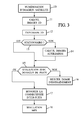
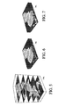
- step 10-11 2D images are obtained, for example those illustrated on the Figures 4A-E .
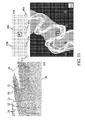
- step 12 is performed to assemble a drive image, as illustrated by the Figures 5-7 .
- obtaining the 2D images begins with the digitization of 10 satellite images that have been taken in a suitable region of the globe. This region is chosen by geological experts for its supposed similarity, in terms of sedimentary behavior, with that where the geological area studied was formed.
- step 12 the digitized 2D images are stacked in the vertical direction ( figure 5 ). It results ( figure 6 ) a 3D image to which another processing, able to use a pseudo-process algorithm, is applied to extrapolate the 3D geological body shape.
- This training image is tested in step 13 to verify stationarity, i.e. if it has a spatial uniformity in terms of orientation or facies proportion. If the image is not stationary, auxiliary training images representing spatial trends are generated from the training image. Auxiliary training images may include drifts regarding facies proportions, azimuths, geological body sizes. They are built semi-automatically in step 14, for example according to the technique described in the aforementioned article by T. L. Chugunova & L.Y. Hu, and then allow to perform the MPS simulation in step 18 despite the non-stationarity of the drive image.
- step 15 of the figure 3 the 3D drive image generated in step 13 is evaluated against available data at one or more wells that drilled in the tank area and in which measurements and samplings were made. A number of statistical consistency criteria between the training image and the well data are evaluated. If one or more of these criteria are poorly verified, the training image is rejected in step 16, and another training image will be generated, for example by modifying the previous training image or starting over again. a method 10-14 similar to that described above. This other training image will be tested again until a satisfactory training image is obtained against the evaluated criteria.
- Another possibility at the end of step 15 is to present the user with the evaluation results of the criteria taken into account, to let the user decide on the results if the training image can be accepted. or not for MPS simulation.
- Step 15 may include an intra-well check relating to the multipoint statistic in parallel with the wells. This can be done on the basis of the distribution of runs, as illustrated by the Figures 8A-B , or Multipoint Density Function (MPDF), as illustrated by the figure 9 (see the aforementioned article by JB Boisvert, J. Pyrcz and CV Deutsch).
- MPDF Multipoint Density Function
- Series distribution is a statistical measure of the vertical extent of facies along a well. For each facies, we count the number consecutive blocks along the wells that have this facies. By block is meant here the number of layers of the reservoir grid which have the facies considered at their intersection with the well. For example, along the well schematized on the figure 8A , there is 1 series of 3 blocks, 2 sets of 2 blocks and 4 sets of 1 block. The numbers recorded are noted on a diagram such as that of the Figure 8B , where the size of the series is plotted on the abscissa. The same reading is made along the vertical columns of the training image defined on the regular grid of cells. The two diagrams obtained are compared and the distance between them gives an indication of the capacity of the training image to account for the vertical extent of the facies along the wells. If the distance is too large, the training image may be rejected.
- the Multipoint Density Function is another multipoint statistical measure along the wells that can be estimated in step 15 on the one hand from the well data on the reservoir grid and on the other hand according to the training image along the vertical columns of the regular grid of cells.
- MPDF is a count of the number of occurrences of different 1D facies patterns along the wells.
- the figure 9 gives a simplified representation in the case of patterns on three layers among two types of facies. A comparison of the number of occurrences of the different patterns along the wells and in the training image thus makes it possible to evaluate the statistical relevance of the training image with a view to informing the user or rejecting the image. drive if necessary.
- Step 15 may further comprise an inter-well verification, the purpose of which is to verify that the training image has, along its I, J layers, two-dimensional facies patterns which correspond to two-dimensional patterns observed in the wells along the geological horizons Ir, Jr of the reservoir grid.
- inter-well verification the purpose of which is to verify that the training image has, along its I, J layers, two-dimensional facies patterns which correspond to two-dimensional patterns observed in the wells along the geological horizons Ir, Jr of the reservoir grid.
- each two-dimensional pattern is defined along any geological horizon.
- the two-dimensional pattern contains the type of facies estimated geological value for the cell based on logs recorded in the well or, if applicable, based on samples taken from the well.
- the Figure 10 (a) shows a seismic horizon 20 of the reservoir grid crossed by four wells 21-24.
- Four types of facies were respectively determined on the seismic horizon from the measurements and samples made in the four wells 21-24.
- the seismic horizon 20 is "flattened” to reorganize the indexes of these cells according to the regular grid I, J by compensating the deformations of the seismic horizon.
- This makes it possible to extract the two-dimensional pattern in the form represented on the Figure 10 (c) where the four facies types identified at the wells are designated 1-4.
- This two-dimensional pattern composed of several types of facies located on the wells, is identified by the position of the regular grid cell which contains the center of gravity of the four wells, marked by an "X" on the Figure 10 (c) .
- a scan is performed to count, in the training image, the occurrences of this two-dimensional pattern.
- the sweep moves the two-dimensional pattern onto the regular grid.
- the cell containing the x centroid of the wells is aligned with a reference cell of the grid of the training image, whereas the cells making up the two-dimensional pattern are aligned on target cells of the grid of the training image. If the facies types of the training image in these four target cells coincide with those of the two-dimensional pattern, a counter is incremented.
- the value of the counter is compared to the number of scanned positions, and the ratio between this counter and this number is used to evaluate the ability of the training image to report well correlations along the seismic horizons as part of the inter-well verification.
- the Figure 11 (a) shows another, more complex example of horizon seismic 30 crossed by six wells 31-36 drilled in the studied area of the basement.
- the Figure 11 (b) shows the same horizon 30 whose cells have been re-arranged in regular arrangement, which makes it possible to define a two-dimensional pattern composed of six types of facies 41a, 42b, 43b, 44c, 45a, 46a respectively placed on the positions of the six wells 31-36 along the horizon, which positions generally have a barycenter B.
- the suffix "a” refers to the type of "alluvial plain” facies found on the horizon at wells 31, 35 and 36
- the suffix "b” refers to the type of facies “sandy deposit” found on the horizon at well 32 and 33
- the suffix "c” refers to the type of "channel” facies found at well 44 in the particular example of horizon 30 of the Figure 11 (a) .
- This two-dimensional pattern of six types of facies finds an occurrence in the training image layer that is drawn on the Figure 11 (c) when the center of gravity B is positioned as shown.
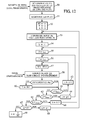
- the figure 12 shows a possible flow diagram of an inter-well verification procedure in one embodiment of the invention.
- the well data which may include logs and / or rock samples, are analyzed to associate respective facies types with the cells of the reservoir grid located along the wells that have been drilled in the well. area of interest.
- the analysis can consist of assigning to a particular cell the type of majority facies in the samples taken in this cell, or taking into account physical measurements made in the well.
- the types of facies thus positioned on the wells may later be used, at step 18 of the figure 3 , to start the MPS simulation.
- step 51 the neighboring wells are grouped together to form one or more groups each composed of M wells (M ⁇ 2).
- the number M can vary from one group to another.
- the step 51 can be performed manually by a user, or it can be partly automated using a horizontal distance criterion between wells.
- a pattern M q is constructed at step 53 of the way illustrated above with reference to Figures 10 (c) and 11 (b) .
- the pattern M q is composed of a number M of facies types arranged on a regular 2D grid. These types of facies will then be identified by their relative positions with respect to the centroid B q , also calculated in step 53, between the positions of the wells of the group considered on the regular 2D grid.
- Three nested loops are then executed to scan the drive image for occurrences of the pattern M q that has just been constructed. These three loops are successively initialized in steps 54, 55 and 56 where the indexes k, j and i are respectively initialized to the values 1, j min and i min .
- the index k numbers the layers of the drive image, while the indexes i, j number cells along both dimensions along the layers.
- the values i min and j min are chosen according to the size of the pattern M q so that it can be superimposed entirely on the layer of the training image.
- the counter NT is incremented by one unit in step 57.
- step 58 the position B q of the center of gravity is aligned with that i, j, k of the current reference cell in the training image, which makes it possible to verify in step 59 whether the pattern M q matches the types of facies encountered in the position-driving image. corresponding target cells.
- the counter N is incremented by one unit in step 60.
- an end of loop test 61 is performed to compare the index i to its maximum value i max (depending again on the size of the pattern M q ).
- the layer index k is incremented by one in step 66 and an additional iteration is performed from step 55 to scan the new layer.
- the value of this ratio ⁇ informs about the probability that there are encountered in the drive image the 2D facies patterns that can be determined between neighboring wells according to the measurements.
- the higher values of ⁇ validate the training image from this point of view, while the lower values would rather encourage the rejection of the training image.
- the evaluation may comprise the comparison of ⁇ with a predefined threshold, for example of the order of a few%. It may also consist in presenting to the user a score, proportional to ⁇ , that this one can take into account together with other scores, resulting for example from intra-well checks of the kind of those illustrated with reference to Figures 8 and 9 .
- the ratio ⁇ may be calculated for each well group formed in step 51.
- the comparison threshold for interwell verification may depend on the number of wells in the group under consideration.
- step 17 is to ensure that the connectivity between the wells is honored.
- the engineers retrieve dynamic information that provides information on the communications between wells, allowing flows of fluid between them. This information can result from interference testing or simply observing pressures and flows over time.
- the purpose of step 17 is to take these observations into account in order to initialize the MPS simulation carried out at step 18.
- the figure 13 shows, by way of example, two groups of cells comprised in the same layer of the reservoir grid, namely a first group of three cells 80 included in a rectangular array 81 and a second group of two cells 83 comprised in a rectangular array 82.
- the layer of the reservoir grid is represented flat for a constant Kr layer index and variable horizontal indexes Ir, Jr.
- the three cells 80 of the group included in the rectangular assembly 81 are situated at the intersection of the layer of the reservoir grid with the wells of a group of three communicating wells.
- the two cells 83 of the group included in the rectangular assembly 82 are located at the intersection of the layer of the reservoir grid with the wells of another group of two communicating wells.
- the identification of such groups of communicating wells is carried out at step 90 shown in FIG. figure 16 .
- the connectivity is observed between different cells belonging to several wells of the group from the dynamic observations made inside these wells when they are tested or exploited.
- cells in a group are represented as belonging to the same layer of the reservoir grid. However, it will be understood that they can be located in different layers, in which case the rectangular sets 81, 82 are generalized to become parallelepiped sets.
- ig, j the horizontal dimensions of the smallest parallelepipedal assembly 81, 82 containing these cells, and kg the dimension vertical of this set.
- the processing refers to a rectangular window 84, or parallelepipedal if kg> 1, which traverses the training image during the scan 91-104.
- the rectangular window 84 shown on the figure 14 corresponds to the rectangular set 81 of the figure 13 .
- the positions 85 which correspond, in the reservoir grid, to the positions of the cells 80 of the group identified in step 90.
- Reference 86 shows a position where the rectangular window 84 is aligned with a set of cells compatible with the 80 cell group of the figure 13
- the reference 87 shows a set of cells compatible with the group of cells 83 of the figure 13 .
- the scan 91-104 comprises three nested loops successively initialized in steps 91, 92 and 93 where the indexes k, j and i are initialized to 1.
- the index k numbers the layers of the drive image, while the indexes i, I number the cells along both dimensions along the layers.
- step 94 if the related set [i, i + i g [x [j, j + i g [x [k, k + k g [covered in the drive image by the window, here in the form of a rectangular parallelepiped, communicates with each other the cells marked as corresponding to the cells of the group identified in step 90, that is to say if Rectangular parallelepiped has a related subset of cells having permeable facies types in the training image and including the labeled cells.
- a rectangular parallelepiped compatible thumbnail (or patch) is detected in the training image and the number n of cells of this thumbnail [i, i + i g [x [j, j + i g [x [k, k + k g [whose type of facies is permeable in the training image is counted in step 95.
- This number of permeable cells in the compatible thumbnails detected in the training image is the subject of a histogram calculation.
- the values H (1), H (2), ... of the histogram H are initialized to 0 before step 91.
- the index c receives the value H (n) +1 at step 96 and the current position (i, j, k) of the scan is assigned to an index p (n, c) identifying the position of the ith compatible thumbnail detected in the image of training (step 97).
- an end-of-loop test 99 is performed to compare the index i with its maximum value i m (i m + i g is the dimension of the image drive along the direction I). If i ⁇ i m , the index i is incremented by one unit in step 100 and an additional iteration in the inner loop is performed from step 94.
- a second end-of-loop test 101 is performed to compare the index j to its maximum value j m (j m + j g is the dimension of the training image along the direction J).
- step 102 If j ⁇ j m , the index j is incremented by one unit at step 102 and an additional iteration is performed from step 93.
- the histogram H (n) for the group of wells considered is then completed. It gives the number of compatible thumbnails found during the scan for each number n of permeable cells. It can be expressed equivalently in terms of the volume of permeable facies (by multiplying n by the elementary volume of a cell) or in terms of the proportion of permeable facies (by dividing n by igxjgxkg). This histogram can be exploited to select a compatible thumbnail that will be applied to the initialization of the MPS simulation to honor inter-sink connectivity.
- the scanning of the driving image for a group of connected wells is followed by a step 105 of choosing a number n (or equivalently of a permeable facies volume, or a proportion of permeable facies ).
- This choice is made according to the statistics revealed by the histogram H (n). For example, the average value or the median of the distribution given by the histogram H (n) can be chosen for n.
- the choice may also take into account a scenario chosen to execute the MPS simulation of step 18. For example, an optimistic scenario may favor the choice of a relatively high number n, whereas a pessimistic scenario may favor the choice. of a relatively low number n.
- a compatible thumbnail is chosen, for example by random drawing among the thumbnails detected with the proportion of permeable facies retained in step 105. This may consist of drawing a number c and taking the thumbnail selected at the position p (n, c) in the image drive.
- the figure 15 shows part of the initialization image corresponding to the Figures 13 and 14 .
- This initialization image defined on the reservoir grid comprises (i) a sticker 88 corresponding to the sticker 86 of the figure 14 stalled on the position of the group of three cells 80 included in the rectangular assembly 81 of the figure 13 and (ii) another sticker 89 corresponding to the sticker 87 of the figure 14 stalled on the position of the group of two cells 83 included in the rectangular assembly 82 of the figure 13 .
- step 18 the MPS simulation is performed to build, on the reservoir grid, the image modeling the studied area of the subsoil.
- the MPS simulation proceeds, in a manner known per se, by propagation from the initialization image by using the training image as a statistical reference.
- the MPS simulation and the preliminary preparation of the training images can be implemented using one or more computers.
- Each computer may comprise a processor type calculation unit, a memory for storing data, a permanent storage system such as one or more hard disks, communication ports for managing communications with external devices, in particular for retrieving data from external devices. Satellite images and well data, and user interfaces such as a screen, a keyboard, a mouse, etc.
- the calculations and steps of the above described above are performed by the processor (s) using software modules that can be stored as program instructions or as readable code.
- the computer and executable by the processor on a computer-readable recording medium such as read-only memory (ROM), random access memory (RAM), CD-ROMs, magnetic tapes, floppy disks and optical data storage devices.
Landscapes
- Engineering & Computer Science (AREA)
- Physics & Mathematics (AREA)
- General Physics & Mathematics (AREA)
- Software Systems (AREA)
- Life Sciences & Earth Sciences (AREA)
- Remote Sensing (AREA)
- Theoretical Computer Science (AREA)
- General Life Sciences & Earth Sciences (AREA)
- Geophysics (AREA)
- Geometry (AREA)
- Acoustics & Sound (AREA)
- Environmental & Geological Engineering (AREA)
- Geology (AREA)
- Artificial Intelligence (AREA)
- Mathematical Physics (AREA)
- Medical Informatics (AREA)
- Computer Vision & Pattern Recognition (AREA)
- Data Mining & Analysis (AREA)
- Evolutionary Computation (AREA)
- General Engineering & Computer Science (AREA)
- Computing Systems (AREA)
- Computer Graphics (AREA)
- Image Processing (AREA)
- Image Analysis (AREA)
Description
La présente invention concerne les techniques géostatistiques multipoint utilisées pour construire des modèles géologiques pour représenter des zones du sous-sol.The present invention relates to multipoint geostatistical techniques used to construct geological models to represent subsoil areas.
Les modèles géologiques sont des outils très utiles à l'étude du sous-sol, en particulier pour l'exploration ou l'exploitation de champs d'hydrocarbures. On essaie de construire un modèle géologique représentant au mieux la structure et le comportement d'un réservoir à partir de mesures effectuées soit en surface (notamment des mesures sismiques) soit dans des puits (logs), ou encore à partir d'observations faites sur des carottes prélevées dans les puits. Bien entendu, même lorsqu'il est effectué de grandes quantités de mesures et de prélèvements, la construction d'un modèle tridimensionnel traduisant très fidèlement la structure et le comportement de la zone étudiée du sous-sol n'est pas un objectif réaliste. C'est pourquoi on a recours à des méthodes statistiques pour la construction de ces modèles.Geological models are very useful tools for studying the subsoil, especially for the exploration or exploitation of hydrocarbon fields. We try to build a geological model that best represents the structure and behavior of a reservoir from measurements made either on the surface (including seismic measurements) or in wells (logs), or from observations made on carrots taken from the wells. Of course, even when large amounts of measurements and samples are taken, the construction of a three-dimensional model very accurately reflecting the structure and behavior of the studied sub-soil area is not a realistic goal. This is why statistical methods are used to construct these models.
Les méthodes géostatistiques traditionnelles reposent sur l'utilisation de variogrammes qui sont des mesures de variabilité spatiale à deux points. Ces méthodes traditionnelles sont très limitées, notamment quant à leur capacité à représenter la topologie parfois complexe de la zone étudiée. Les méthodes multipoint ont été proposées à partir des années 1990 pour surmonter ces limitations.Traditional geostatistical methods rely on the use of variograms that are two-point spatial variability measures. These traditional methods are very limited, especially as to their ability to represent the sometimes complex topology of the study area. Multipoint methods have been proposed since the 1990s to overcome these limitations.
Les techniques statistiques multipoint (MPS, "Multi-Point Statistics") permettent de modéliser les hétérogénéités géologiques de telle façon qu'on puisse reproduire des systèmes naturels en rendant mieux compte des incertitudes du modèle.Multipoint Point Statistics (MPS) are used to model geological heterogeneities so that natural systems can be reproduced by better accounting for model uncertainties.
Les données d'entrée des techniques de simulation MPS incluent des images d'entraînement dont le choix joue un rôle important dans la fiabilité du modèle obtenu. Une image d'entraînement est définie sur une grille tridimensionnelle (3D). Elle est choisie de manière à représenter des motifs d'hétérogénéités géologiques qu'on peut s'attendre à rencontrer dans le réservoir (voir
Dans les débuts des techniques MPS, on utilisait une image d'entraînement stationnaire formant une représentation conceptuelle d'un système sédimentaire, obtenue à partir d'un croquis établi par un géologue ou à partir d'une simulation à base d'objets. Des algorithmes plus récents ont permis d'effectuer des simulations MPS en utilisant des images d'entraînement non-stationnaires, en combinant celles-ci avec des images d'entraînement auxiliaires (voir
Les images d'entraînement peuvent notamment correspondre à une représentation simplifiée d'un analogue contemporain, obtenue par une technique de traitement d'image appliquée à des photographies prises par satellite dans une région du globe qui, de l'avis d'experts géologues, présente des caractéristiques similaires à celles de la région où se sont autrefois formés les dépôts sédimentaires se trouvant dans la zone étudiée du sous-sol. Par exemple, différentes images satellite sont traitées puis empilées pour former une représentation tridimensionnelle qui servira d'image d'entraînement.In particular, the training images may be a simplified representation of a contemporary analogue, obtained by an image processing technique applied to satellite photographs taken in a region of the world which, in the opinion of geological experts, has characteristics similar to those of the area where sedimentary deposits were previously formed in the studied subsoil area. For example, different satellite images are processed and stacked to form a three-dimensional representation that will serve as a training image.
Très souvent, l'étude d'une zone géologique particulière comporte le forage d'un ou plusieurs puits dans cette zone pour y effectuer des mesures (logs) et/ou des prélèvements. Il est alors possible de vérifier si l'image d'entraînement 3D semble cohérente avec les données de puits disponibles, afin de valider l'image d'entraînement ou d'indiquer qu'elle devrait être modifiée. En effet, une image d'entraînement qui ne serait pas cohérente avec les données de puits est susceptible de fournir une mauvaise représentation des hétérogénéités durant la simulation.Very often, the study of a particular geological area involves the drilling of one or more wells in this area to perform measurements (logs) and / or sampling. It is then possible to check whether the 3D training image seems consistent with the available well data, in order to validate the training image or indicate that it should be modified. Indeed, a training image that is not consistent with the well data is likely to provide a poor representation of the heterogeneities during the simulation.
Des méthodes applicables à la validation des hétérogénéités verticales sur des images d'entraînement ont été proposées par
Un but de la présente invention est d'enrichir les méthodes de génération et de validation d'images d'entraînement. Il est notamment souhaitable de pouvoir valider une image d'entraînement par rapport à des données de puits sans se limiter à des estimations statistiques parallèlement à un puits.An object of the present invention is to enrich the methods of generating and validating training images. It is particularly desirable to be able to validate a training image with respect to well data without being limited to statistical estimates in parallel with a well.
Selon invention, il est proposé un procédé de préparation d'une image d'entraînement pour la modélisation d'une zone du sous-sol par une technique géostatistique multipoint. Ce procédé comprend:
- construire une image d'entraînement sur une première grille de cellules tridimensionnelle, l'image d'entraînement donnant, pour chaque cellule de la première grille tridimensionnelle, un type respectif de faciès géologique affecté à cette cellule; et
- vérifier la représentativité de l'image d'entraînement par rapport à des données de puits obtenues à partir d'observations faites dans plusieurs puits qui ont été forés dans la zone du sous-sol, les données de puits faisant référence à une seconde grille de cellules tridimensionnelle dont la morphologie est adaptée à des horizons géologiques estimés dans la zone du sous-sol, les données de puits incluant des types de faciès géologique respectivement estimés d'après les observations pour des cellules de la seconde grille tridimensionnelle situées le long des puits.
- constructing a training image on a first three-dimensional cell grid, the training image giving, for each cell of the first three-dimensional grid, a respective type of geological facies assigned to that cell; and
- verify the representativeness of the training image with respect to well data obtained from observations made in several wells that have been drilled in the subsoil zone, the well data referring to a second grid of three-dimensional cells whose morphology is adapted to estimated geological horizons in the subsoil zone, the well data including geological facies types respectively estimated from observations for cells of the second three-dimensional grid located along the wells .
La vérification de représentativité de l'image d'entraînement par rapport aux données de puits comporte une vérification inter-puits qui comprend:
- identifier des motifs bidimensionnels dans les données de puits, chaque motif bidimensionnel étant défini le long d'un horizon géologique respectif et incluant, dans une cellule contenant l'intersection d'un puits avec ledit horizon géologique dans la seconde grille tridimensionnelle, le type de faciès géologique estimé pour cette cellule; et
- compter, dans l'image d'entraînement, les occurrences des motifs bidimensionnels identifiés.
- identifying two-dimensional patterns in the well data, each two-dimensional pattern being defined along a respective geologic horizon and including, in a cell containing the intersection of a well with said geological horizon in the second three-dimensional grid, the type of geological facies estimated for this cell; and
- counting, in the training image, the occurrences of the two-dimensional patterns identified.
La vérification de représentativité de l'image d'entraînement par rapport aux données de puits n'est pas limitée à une vérification verticale. Une vérification latérale est opérée pour exploiter l'information fournie par les corrélations d'un puits à un autre, grâce à une analyse reposant sur des motifs bidimensionnels pouvant être identifiés pour des groupes de M puits voisins, M étant un nombre choisi supérieur à 1. On augmente aussi ainsi la probabilité que le modèle qui sera généré par la technique MPS représente convenablement la zone étudiée du sous-sol.The representational verification of the training image with respect to the well data is not limited to a vertical verification. A lateral verification is performed to exploit the information provided by the correlations from one well to another, by means of an analysis based on two-dimensional patterns that can be identified for groups of M neighboring wells, where M is a chosen number greater than 1 This also increases the probability that the model that will be generated by the MPS technique adequately represents the studied area of the subsoil.
La vérification inter-puits peut comprendre une validation de l'image d'entraînement lorsque le nombre des occurrences comptées des motifs bidimensionnels identifiés dépasse un seuil, lequel seuil peut être exprimé proportionnellement au nombre de positions possibles du motif bidimensionnel dans l'image d'entraînement.The inter-well verification may include a validation of the training image when the number of counted occurrences of the identified two-dimensional patterns exceeds a threshold, which threshold may be expressed in proportion to the number of possible positions of the two-dimensional pattern in the image of training.
Dans une réalisation, chaque motif bidimensionnel, défini pour des puits croisant un horizon géologique, est repéré par la position de la cellule de la seconde grille tridimensionnelle contenant le barycentre de ces puits le long de l'horizon géologique considéré. Le comptage, dans l'image d'entraînement, des occurrences d'un motif bidimensionnel repéré par la position d'une cellule de barycentre peut alors comprendre:
- balayer l'image d'entraînement, chaque étape du balayage plaçant le motif bidimensionnel sur la première grille tridimensionnelle en alignant la cellule contenant le barycentre des puits sur une cellule de référence de la première grille tridimensionnelle et les cellules du motif bidimensionnel contenant respectivement les intersections entre les puits et l'horizon géologique sur des cellules-cible de la première grille tridimensionnelle; et
- incrémenter un compteur chaque fois qu'une étape du balayage fait coïncider les types de faciès estimés pour les cellules du motif bidimensionnel avec les types de faciès respectivement affectés aux cellules-cible dans l'image d'entraînement.
- scanning the training image, each step of the scanning placing the two-dimensional pattern on the first three-dimensional grid by aligning the cell containing the barycentre of the wells on a reference cell of the first three-dimensional grid and the cells of the two-dimensional pattern respectively containing the intersections between the wells and the geological horizon on target cells of the first three-dimensional grid; and
- incrementing a counter each time a scan step matches the facies types estimated for the cells of the two-dimensional pattern with the facies types respectively assigned to the target cells in the training image.
La vérification de représentativité de l'image d'entraînement par rapport aux données de puits peut être complétée par une vérification intra-puits comprenant:
- estimer une mesure statistique multipoint, telle qu'une une fonction de densité multipoint (MPDF) ou une distribution de séries ("distribution of runs"), le long de chaque puits parmi les données de puits;
- estimer la même mesure statistique multipoint le long de colonnes verticales de la première grille de cellules tridimensionnelle; et
- comparer les deux mesures statistiques multipoint estimées.
- estimating a multipoint statistical metric, such as a multipoint density function (MPDF) or a distribution of runs ("distribution of runs"), along each well of the well data;
- estimating the same multipoint statistical measure along vertical columns of the first three-dimensional cell grid; and
- compare the two estimated multipoint statistical measures.
Un autre aspect de la présente invention se rapporte à un système de traitement de données adapté à la préparation d'une image d'entraînement pour la modélisation d'une zone du sous-sol par une technique géostatistique multipoint. Le système comprend des ressources informatiques configurées pour mettre en oeuvre un procédé tel que défini ci-dessus.Another aspect of the present invention relates to a data processing system adapted to the preparation of a training image for modeling a subsoil area by a multipoint geostatistical technique. The system comprises computer resources configured to implement a method as defined above.
Un autre aspect encore de la présente invention se rapporte à un programme d'ordinateur pour un système de traitement de données, le programme comprenant des instructions pour mettre en oeuvre un procédé tel que défini ci-dessus lorsqu'il est exécuté sur une unité de calcul du système de traitement de données. Un support d'enregistrement lisible par ordinateur, sur lequel est enregistré un tel programme est également proposé.Yet another aspect of the present invention relates to a computer program for a data processing system, the program comprising instructions for implementing a method as defined above when executed on a data processing unit. calculation of the data processing system. A computer readable recording medium on which such a program is recorded is also provided.
D'autres particularités et avantages de la présente invention apparaîtront dans la description ci-après d'un exemple de réalisation non limitatif, en référence aux dessins annexés, dans lesquels :
- les
figures 1 et 2 sont des illustrations schématiques d'une grille régulière et d'une grille réservoir, respectivement; - la
figure 3 est un organigramme d'un exemple de réalisation d'un procédé selon l'invention; - les
figures 4A-4E montre des exemples d'images satellite prétraitées pour l'assemblage d'une image d'entraînement à trois dimensions; - les
figures 5 à 7 sont des schémas illustrant l'assemblage de l'image d'entraînement 3D; - les
figures 8A-B sont des diagrammes illustrant un premier exemple de mesure statistique multipoint; - la
figure 9 est un diagramme illustrant un second exemple de mesure statistique multipoint; - la
figure 10 illustre une manière de vérifier la représentativité de l'image d'entraînement par rapport à des données de puits; - la
figure 11 est une autre illustration de la vérification de représentativité de l'image d'entraînement par rapport aux données de puits; - la
figure 12 est un organigramme un exemple de procédure applicable dans une vérification inter-puits d'une image d'entraînement; - les
figures 13 à 15 sont des schémas illustrant une technique permettant de prendre en compte des informations de connectivité entre puits dans l'initialisation d'une simulation MPS; et - la
figure 16 est un organigramme montrant une façon de mettre en oeuvre la technique illustrée par lesfigures 13-15 .
- the
Figures 1 and 2 are schematic illustrations of a regular grid and a reservoir grid, respectively; - the
figure 3 is a flowchart of an exemplary embodiment of a method according to the invention; - the
Figures 4A-4E shows examples of pretreated satellite images for assembling a three-dimensional training image; - the
Figures 5 to 7 are diagrams illustrating the assembly of the 3D training image; - the
Figures 8A-B are diagrams illustrating a first example of multipoint statistical measurement; - the
figure 9 is a diagram illustrating a second example of multipoint statistical measurement; - the
figure 10 illustrates a way of verifying the representativeness of the training image with respect to well data; - the
figure 11 is another illustration of the representational verification of the training image with respect to the well data; - the
figure 12 is a flowchart an example of a procedure applicable in an inter-well check of a training image; - the
Figures 13 to 15 are diagrams illustrating a technique for taking into account well connectivity information in the initialization of an MPS simulation; and - the
figure 16 is a flowchart showing a way to implement the technique illustrated by theFigures 13-15 .
Les techniques de statistique multipoint (MPS) se sont développées au cours des vingt dernières années. Les faciès de la zone géologique considérée sont modélisés pixel par pixel sur une grille de cellules tridimensionnelle dont la morphologie est adaptée aux horizons géologiques dans la zone à modéliser. Cette grille 3D est appelée grille réservoir. La simulation MPS affecte à chaque pixel de la grille réservoir une valeur de faciès, par exemple un nombre entier, correspondant à une codification de quelques types de faciès qu'on s'attend à trouver dans la zone à modéliser. Par exemple, dans un environnement fluviatile, les types de faciès peuvent être chenal, plaine alluviale, dépôt sableux, ébrasement de crevasse, etc.Multipoint statistics (MPS) techniques have developed over the last twenty years. The facies of the geological zone considered are modeled pixel by pixel on a grid of three-dimensional cells whose morphology is adapted to the geological horizons in the zone to be modeled. This 3D grid is called tank grid. The MPS simulation assigns to each pixel of the reservoir grid a facies value, for example an integer, corresponding to a codification of some types of facies that are expected to be found in the zone to be modeled. For example, in a fluvial environment, facies types may be channel, alluvial plain, sandy deposit, crevasse splay, etc.
La mise en oeuvre d'une technique MPS nécessite de disposer d'une image d'entraînement 3D dont le contenu statistique soit représentatif de la zone à modéliser. Cette image d'entraînement est typiquement définie sur une première grille de cellules tridimensionnelle de forme régulière, et contient de l'information statistique sur les faciès sédimentaires à l'échelle des corps géologiques ("geobody").The implementation of an MPS technique requires having a 3D training image whose statistical content is representative of the area to be modeled. This training image is typically defined on a first grid of three-dimensional cells of regular shape, and contains statistical information on sedimentary facies on the scale of geological bodies ("geobody").
La simulation MPS peut consister à balayer l'image d'entraînement à l'aide d'une fenêtre rectangulaire, à y repérer les différentes configurations de faciès rencontrées et à les organiser en une liste ou un arbre de recherche. Ensuite, à partir des cellules initialement renseignées de la grille réservoir (par exemple d'après des prélèvements effectués dans des puits), l'algorithme parcourt la grille réservoir et récupère les configurations compatibles dans l'arbre de recherche puis tire des valeurs de faciès issues de ces configurations selon leur fonction de distribution probabiliste. Il construit ainsi de proche en proche un modèle de réservoir dont les corrélations spatiales de faciès sont statistiquement semblables à celles de l'image d'entraînement.The MPS simulation may consist of scanning the training image using a rectangular window, identifying the different facies configurations encountered and organizing them into a list or a search tree. Then, from the initially filled cells of the reservoir grid (for example from samples taken in wells), the algorithm traverses the reservoir grid and retrieves the compatible configurations in the search tree and then draws facies values. from these configurations according to their probabilistic distribution function. He thus constructs, step by step, a reservoir model whose spatial correlations of facies are statistically similar to those of the training image.
Bien entendu, la qualité de la modélisation dépend fortement de la capacité de l'image d'entraînement à représenter convenablement la statistique de la zone modélisée.Of course, the quality of the modeling strongly depends on the ability of the training image to adequately represent the statistics of the modeled area.
Une grille régulière de cellules telle qu'illustrée sur la
Une grille réservoir (
En général, le nombre de couches dans la grille de l'image d'entraînement est inférieur au nombre de couches dans la grille réservoir.In general, the number of layers in the grid of the training image is smaller than the number of layers in the reservoir grid.
Un mode de réalisation du procédé de préparation de l'image entraînement en vue de la simulation MPS de la zone du sous-sol est présenté en référence à la
Dans l'exemple de la
La numérisation semi-automatique d'images satellite par des techniques de traitement d'image permet d'extraire rapidement les parties d'une photographie qui sont significatives en termes de corps de dépôt sédimentaire. Ces techniques de traitement d'image reposent sur des algorithmes tels que la détection de bords de Canny (
À l'étape 12, les images 2D numérisées sont empilées selon la direction verticale (
Cette image d'entraînement est testée à l'étape 13 pour vérifier sa stationnarité, c'est-à-dire si elle présente une uniformité spatiale en termes d'orientation ou de proportion de faciès. Si l'image n'est pas stationnaire, des images d'entraînement auxiliaires représentant les tendances spatiales sont générées à partir de l'image d'entraînement. Les images d'entraînement auxiliaires peuvent inclure des dérives concernant les proportions de faciès, les azimuts, les tailles de corps géologiques. Elles sont construites de manière semi-automatique à l'étape 14, par exemple selon la technique décrite dans l'article précité de T.L. Chugunova & L.Y. Hu, et permettront ensuite d'effectuer la simulation MPS à l'étape 18 malgré la non-stationnarité de l'image entraînement.This training image is tested in
À l'étape 15 de la
L'étape 15 peut comporter une vérification intra-puits se rapportant à la statistique multipoint parallèlement aux puits. Ceci peut notamment être effectué sur la base de la distribution de séries ("distribution of runs"), comme illustré par les
La distribution de séries est une mesure statistique de l'étendue verticale des faciès le long d'un puits. Pour chaque faciès, on compte le nombre de blocs consécutifs le long des puits qui présentent ce faciès. Par bloc on entend ici le nombre de couches de la grille réservoir qui ont le faciès considéré à leur intersection avec le puits. Par exemple, le long du puits schématisé sur la
La fonction de densité multipoint (MPDF) est une autre mesure statistique multipoint le long des puits qui peut être estimée à l'étape 15 d'une part d'après les données de puits sur la grille réservoir et d'autre part d'après l'image d'entraînement le long des colonnes verticales de la grille régulière de cellules. La MPDF est un décompte des nombres d'occurrences de différents motifs 1 D de faciès le long des puits. La
L'étape 15 peut en outre comporter une vérification inter-puits dont le but est de vérifier que l'image d'entraînement présente, le long de ses couches I, J, des motifs bidimensionnels de faciès qui correspondent à des motifs bidimensionnels observés dans les puits le long des horizons géologiques Ir, Jr de la grille réservoir.
Pour effectuer cette vérification inter-puits, on commence par identifier des motifs bidimensionnels dans les données de puits. Chaque motif bidimensionnel est défini le long d'un horizon géologique quelconque. Dans une cellule de la grille réservoir où se trouve l'intersection d'un puits avec l'horizon géologique considéré, le motif bidimensionnel contient le type de faciès géologique estimé pour la cellule d'après les logs qui ont été enregistrés dans le puits ou, le cas échéant, d'après l'examen d'échantillons prélevés dans le puits.To perform this inter-well verification, we first identify two-dimensional patterns in the well data. Each two-dimensional pattern is defined along any geological horizon. In a cell of the reservoir grid where there is the intersection of a well with the geological horizon considered, the two-dimensional pattern contains the type of facies estimated geological value for the cell based on logs recorded in the well or, if applicable, based on samples taken from the well.
Par exemple, la
Pour chaque motif bidimensionnel de faciès qui a ainsi été extrait à partir des données de puits, un balayage est effectué pour compter, dans l'image d'entraînement, les occurrences de ce motif bidimensionnel. Pour chaque couche (d'index K) de l'image d'entraînement, le balayage déplace le motif bidimensionnel sur la grille régulière. À chacune des étapes successives de ce déplacement (par exemple l'étape représentée sur la
À la fin de cette opération, la valeur du compteur est comparée au nombre de positions balayées, et le rapport entre ce compteur et ce nombre sert à évaluer la capacité de l'image d'entraînement à rendre compte des corrélations entre puits le long des horizons sismiques dans le cadre de la vérification inter-puits.At the end of this operation, the value of the counter is compared to the number of scanned positions, and the ratio between this counter and this number is used to evaluate the ability of the training image to report well correlations along the seismic horizons as part of the inter-well verification.
La
La
Ensuite (étape 51), les puits voisins sont regroupés pour former un ou plusieurs groupes composés chacun de M puits (M ≥ 2). Le nombre M peut varier d'un groupe à un autre. L'étape 51 peut être effectuée manuellement par un utilisateur, ou elle peut être en partie automatisée à l'aide d'un critère de distance horizontale entre puits.Then (step 51), the neighboring wells are grouped together to form one or more groups each composed of M wells (M ≥ 2). The number M can vary from one group to another. The
Le comptage des occurrences des motifs bidimensionnels est alors initialisé à l'étape 52, par exemple en affectant des valeurs nulles aux compteurs NT et N et la valeur 1 à l'index de motif q. Un motif Mq est construit à l'étape 53 de la manière illustrée ci-dessus en référence aux
Trois boucles imbriquées sont ensuite exécutées pour balayer l'image entraînement en vue d'y détecter les occurrences du motif Mq qui vient d'être construit. Ces trois boucles sont successivement initialisées aux étapes 54, 55 et 56 où les index k, j et i sont respectivement initialisés aux valeurs 1, jmin et imin. L'index k numérote les couches de l'image entraînement, tandis que les index i, j numérotent les cellules suivant les deux dimensions le long des couches. Les valeurs imin et jmin sont choisies en fonction de la taille du motif Mq afin que celui-ci puisse être superposé en totalité sur la couche considérée de l'image d'entraînement. À chaque position d'une cellule de référence i, j, k au cours du balayage, le compteur NT est incrémenté d'une unité à l'étape 57. Puis (étape 58), la position Bq du barycentre est alignée sur celle i, j, k de la cellule de référence courante dans l'image d'entraînement, ce qui permet de vérifier à l'étape 59 si le motif Mq concorde avec les types de faciès rencontrés dans l'image d'entraînement aux positions des cellules-cible correspondantes. Lorsqu'il y a concordance, une occurrence du motif Mq est détectée et le compteur N est incrémenté d'une unité à l'étape 60. Après l'étape 60, ou en cas de non-concordance du motif à l'étape 59, un test de fin de boucle 61 est effectué pour comparer l'index i à sa valeur maximale imax (dépendant à nouveau de la taille du motif Mq). Si i < imax, l'index i est incrémenté d'une unité à l'étape 62 et une itération supplémentaire dans la boucle interne est effectuée à partir de l'étape 57. Quand i = imax au test 61, un deuxième test de fin de boucle 63 est effectué pour comparer l'index j à sa valeur maximale jmax (dépendant de la taille du motif Mq). Si j < jmax, l'index j est incrémenté d'une unité à l'étape 64 et une itération supplémentaire est effectuée à partir de l'étape 56. Quand j = jmax au test 63, un troisième test de fin de boucle 65 est effectué pour comparer l'index de couche k à sa valeur maximale kmax (nombre de couches dans l'image d'entraînement). Si k < kmax, l'index de couche k est incrémenté d'une unité à l'étape 66 et une itération supplémentaire est effectuée à partir de l'étape 55 pour balayer la nouvelle couche. Quand k = kmax au test 65, il est examiné au test 67 si tous les motifs Mq ont été recherchés dans l'image d'entraînement, c'est-à-dire si l'index de motif q est égal au nombre de motifs possibles Q (égal au nombre de groupes retenus à l'étape 51 multiplié par le nombre de couches dans la grille réservoir). Si q < Q, l'index q est incrémenté d'une unité à l'étape 68 et l'algorithme revient à l'étape 53 pour construire le motif suivant. Les balayages de l'image d'entraînement sont terminés quand q = Q au test 67.Three nested loops are then executed to scan the drive image for occurrences of the pattern M q that has just been constructed. These three loops are successively initialized in
À ce stade, les nombres N et NT sont comparés, par exemple en calculant leur rapport α = N/NT à l'étape 69.At this point, the numbers N and NT are compared, for example by calculating their ratio α = N / NT in
La valeur de ce rapport α renseigne sur la probabilité qu'il y a de rencontrer dans l'image d'entraînement les motifs de faciès 2D qui peuvent être déterminés entre puits voisins d'après les mesures. Les valeurs les plus élevées de α permettent de valider l'image d'entraînement de ce point de vue, tandis que les valeurs les plus basses inciteraient plutôt à rejeter l'image d'entraînement. L'évaluation peut comporter la comparaison de α à un seuil prédéfini, par exemple de l'ordre de quelques %. Elle peut aussi consister à présenter à l'utilisateur un score, proportionnel à α, que celui-ci pourra prendre en compte conjointement à d'autres scores, résultant par exemple de vérifications intra-puits du genre de celles illustrées en référence aux
En variante, le rapport α peut être calculé pour chaque groupe de puits formé à l'étape 51. Le seuil de comparaison pour la vérification inter-puits peut dépendre du nombre de puits dans le groupe considéré.Alternatively, the ratio α may be calculated for each well group formed in
Revenant à la
Les observations dynamiques fournissent de l'information forte sur les communications entre puits. Ces communications révèlent l'existence de trajets d'écoulement entre les puits, composés de roches relativement perméables. Une bonne prise en compte de la connectivité entre puits améliore beaucoup les simulations d'écoulement.Dynamic observations provide strong information on well communications. These communications reveal the existence of flow paths between wells, composed of relatively permeable rocks. A good consideration of the connectivity between wells greatly improves the flow simulations.
La
L'identification de tels groupes de puits communicants est effectuée à l'étape 90 représentée sur la
Pour un groupe g de cellules de la grille réservoir situées le long de plusieurs puits et entre lesquelles des communications hydrodynamiques ont été observées, on note ig, jg les dimensions horizontales du plus petit ensemble parallélépipédique 81, 82 contenant ces cellules, et kg la dimension verticale de cet ensemble. Dans l'exemple de la
Pour chaque groupe de cellules de la grille réservoir identifié à l'étape 90 de la
Le balayage 91-104 consiste à rechercher des vignettes rectangulaires ou parallélépipédiques compatibles avec le groupe de cellules 80. Ces vignettes compatibles sont des ensembles connexes de cellules de la grille régulière qui remplissent deux conditions:
- présenter dans l'image d'entraînement, aux positions marquées 85 qui correspondent aux cellules 80 du groupe, les mêmes types de faciès respectifs que ceux qui ont été déterminés dans les puits pour
ces cellules 80; et - inclure un sous-ensemble connexe de cellules auquel appartiennent celles qui se trouvent aux positions marquées 85 et présentant dans l'image d'entraînement des types de faciès perméables, c'est-à-dire autorisant un écoulement de fluide entre les cellules du groupe.
- show in the training image, at the labeled
positions 85 which correspond to thecells 80 of the group, the same types of facies respective as those determined in the wells for thesecells 80; and - include a related subset of cells to which belong those at
marked positions 85 and having in the drive image permeable facies types, i.e., allowing fluid flow between the cells of the group .
On distingue ainsi au moins deux familles de faciès dans la modélisation: une famille de faciès relativement perméables (1ère famille, par exemple faciès chenal ou dépôt sableux)), laissant s'écouler des fluides tels que de l'huile ou du gaz naturel, et une famille de faciès moins perméables (2ème famille). Ce sont les faciès de la 1ère famille qu'il faut trouver dans les sous-ensembles connexes pour accepter une vignette compatible.We can distinguish at least two families in facies modeling: a family of relatively permeable facies (1 st family, for example channel facies or sandy deposit)), leaving flow of fluids such as oil or natural gas , and a family of less permeable facies ( 2nd family). These are the facies of the 1 st family must be found in the related sub-assemblies to accept compatible thumbnail.
Sur la
Le balayage 91-104 comporte trois boucles imbriquées successivement initialisées aux étapes 91, 92 et 93 où les index k, j et i sont initialisés à 1. L'index k numérote les couches de l'image entraînement, tandis que les index i, j numérotent les cellules suivant les deux dimensions le long des couches. À chaque position i, j, k au cours du balayage, il est examiné à l'étape 94 si l'ensemble connexe [i, i+ig[ x [j, j+ig[ x [k, k+kg[ couvert dans l'image d'entraînement par la fenêtre, ici en forme de parallélépipède rectangle, fait communiquer entre elles les cellules marquées comme correspondant aux cellules du groupe identifié à l'étape 90, c'est-à-dire si ce parallélépipède rectangle a un sous-ensemble connexe de cellules ayant des types de faciès perméables dans l'image d'entraînement et incluant les cellules marquées. Dans l'affirmative, une vignette (ou patch) compatible en forme de parallélépipède rectangle est détectée dans l'image d'entraînement et le nombre n de cellules de cette vignette [i, i+ig[ x [j, j+ig[ x [k, k+kg[ dont le type de faciès est perméable dans l'image d'entraînement est compté à l'étape 95.The scan 91-104 comprises three nested loops successively initialized in
Ce nombre de cellules perméables dans les vignettes compatibles détectées dans l'image d'entraînement fait l'objet d'un calcul d'histogramme. Les valeurs H(1), H(2), ... de l'histogramme H sont initialisées à 0 avant l'étape 91. Après le calcul du nombre n à l'étape 95, l'index c reçoit la valeur H(n)+1 à l'étape 96 et la position courante (i, j, k) du balayage est affectée à un index p(n, c) repérant la position de la c-ième vignette compatible détectée dans l'image d'entraînement (étape 97). L'histogramme est ensuite mis à jour à l'étape 98 en prenant H(n) = c.This number of permeable cells in the compatible thumbnails detected in the training image is the subject of a histogram calculation. The values H (1), H (2), ... of the histogram H are initialized to 0 before
Après l'étape 98, ou lorsque le test de compatibilité 94 est négatif, un test de fin de boucle 99 est effectué pour comparer l'index i à sa valeur maximale im (im+ig est la dimension de l'image d'entraînement le long de la direction I). Si i < im, l'index i est incrémenté d'une unité à l'étape 100 et une itération supplémentaire dans la boucle interne est effectuée à partir de l'étape 94. Quand i = im au test 99, un deuxième test de fin de boucle 101 est effectué pour comparer l'index j à sa valeur maximale jm (jm+jg est la dimension de l'image d'entraînement le long de la direction J). Si j < jm, l'index j est incrémenté d'une unité à l'étape 102 et une itération supplémentaire est effectuée à partir de l'étape 93. Quand j = jm au test 101, un troisième test de fin de boucle 103 est effectué pour comparer l'index de couche k à sa valeur maximale km (km+kg est la dimension de l'image d'entraînement le long de la direction K). Si k < km, l'index de couche k est incrémenté d'une unité à l'étape 104 et une itération supplémentaire est effectuée à partir de l'étape 91. Quand k = km au test 103, le balayage de l'image d'entraînement est terminé.After
L'histogramme H(n) pour le groupe de puits considéré est alors complété. Il donne le nombre de vignettes compatibles trouvées lors du balayage pour chaque nombre n de cellules perméables. Il peut être exprimé de façon équivalente en termes de volume de faciès perméable (en multipliant n par le volume élémentaire d'une cellule) ou en termes de proportion de faciès perméable (en divisant n par igxjgxkg). Cet histogramme peut être exploité pour sélectionner une vignette compatible qui sera appliquée à l'initialisation de la simulation MPS pour honorer la connectivité inter-puits.The histogram H (n) for the group of wells considered is then completed. It gives the number of compatible thumbnails found during the scan for each number n of permeable cells. It can be expressed equivalently in terms of the volume of permeable facies (by multiplying n by the elementary volume of a cell) or in terms of the proportion of permeable facies (by dividing n by igxjgxkg). This histogram can be exploited to select a compatible thumbnail that will be applied to the initialization of the MPS simulation to honor inter-sink connectivity.
Dans l'exemple de la
À l'étape 106, une vignette compatible est choisie, par exemple par tirage au sort parmi les vignettes détectées avec la proportion de faciès perméable retenue à l'étape 105. Ceci peut consister à tirer au sort un nombre c et à prendre la vignette sélectionnée à la position p(n, c) dans l'image d'entraînement.In
Pour initialiser la simulation MPS de l'étape 18 (
- dans les cellules situées le long d'un puits, les types de faciès qui ont été déterminés par les mesures ou prélèvements effectués dans ce puits;
- dans les cellules situées dans les rectangles ou parallélépipèdes correspondant à un groupe de puits connectés identifié à l'étape 90, les types de faciès rencontrés dans l'image d'entraînement dans les cellules correspondantes de la vignette sélectionnée pour ce groupe.
- in cells along a well, the types of facies that were determined by the measurements or samples made in that well;
- in the cells located in the rectangles or parallelepipeds corresponding to a group of connected wells identified in
step 90, the types of facies encountered in the training image in the corresponding cells of the thumbnail selected for this group.
La
À l'étape 18, la simulation MPS est effectuée pour construire, sur la grille réservoir, l'image modélisant la zone étudiée du sous-sol. La simulation MPS procède, de façon connue en soi, par propagation à partir de l'image d'initialisation en utilisant l'image d'entraînement comme référence statistique.In
La simulation MPS et la préparation préalable des images d'entraînement peuvent être mises en oeuvre à l'aide d'un ou plusieurs ordinateurs. Chaque ordinateur peut comprendre une unité de calcul de type processeur, une mémoire pour stocker des données, un système de stockage permanent tel qu'un ou plusieurs disques durs, des ports de communication pour gérer des communications avec des dispositifs externes, notamment pour récupérer les images satellites et les données de puits, et des interfaces utilisateurs comme par exemple un écran, un clavier, une souris, etc.The MPS simulation and the preliminary preparation of the training images can be implemented using one or more computers. Each computer may comprise a processor type calculation unit, a memory for storing data, a permanent storage system such as one or more hard disks, communication ports for managing communications with external devices, in particular for retrieving data from external devices. satellite images and well data, and user interfaces such as a screen, a keyboard, a mouse, etc.
Typiquement, les calculs et les étapes du précédé décrit ci-dessus sont exécutés par le ou les processeurs en utilisant des modules logiciels qui peuvent être stockés, sous forme d'instructions de programmes ou de code lisible par l'ordinateur et exécutable par le processeur, sur un support d'enregistrement lisible par ordinateur tel qu'une mémoire lecture seule (ROM), une mémoire à accès aléatoire (RAM), des CD-ROMs, des bandes magnétiques, des disquettes et des dispositifs optiques de stockage de données.Typically, the calculations and steps of the above described above are performed by the processor (s) using software modules that can be stored as program instructions or as readable code. the computer and executable by the processor, on a computer-readable recording medium such as read-only memory (ROM), random access memory (RAM), CD-ROMs, magnetic tapes, floppy disks and optical data storage devices.
Les modes de réalisation décrits ci-dessus sont des illustrations de la présente invention. Diverses modifications peuvent leur être apportées sans sortir du cadre de l'invention qui ressort des revendications annexées.The embodiments described above are illustrations of the present invention. Various modifications can be made without departing from the scope of the invention which emerges from the appended claims.
Claims (10)
- A method for preparing a training image for modeling an area of the subsoil by a multipoint geostatistical technique, the method comprising:- constructing a training image on a first three-dimensional grid of cells, the training image giving, for each cell of the first grid, a respective type of geological facies assigned to said cell; and- verifying representativeness of the training image with respect to well data obtained from observations conducted in a plurality of wells drilled in the area of the subsoil, the well data referring to a second three-dimensional grid of cells having a morphology adapted to estimated geological horizons in the area of the subsoil, the well data including the types of geological facies that are respectively estimated from the observations for the cells of the second grid located along the wells,
characterized in that the verification of representativeness of the training image with respect to the well data includes an inter-well verification which comprises:- identifying two-dimensional patterns in the well data, each two-dimensional pattern being defined along a respective geological horizon and including, in a cell containing an intersection of a well with said geological horizon in the second grid, the type of geological facies estimated for said cell; and- counting, in the training image, occurrences of the two-dimensional patterns identified. - The method as claimed in claim 1, wherein the inter-well verification further comprises:- validating the training image when the counted number of occurrences of the identified two-dimensional patterns exceeds a threshold.
- The method as claimed in claim 2, wherein said threshold is expressed in proportion to a number of possible positions of the two-dimensional pattern in the training image.
- The method as claimed in any one of the preceding claims, wherein each two-dimensional pattern defined for wells intersecting a geological horizon has a position identified by the position of the cell of the second three-dimensional grid containing a centroid of said wells along said geologic horizon.
- The method as claimed in claim 4, wherein the counting, in the training image, of the occurrences of a two-dimensional pattern positionally identified by the position of a centroid cell comprises:- scanning the training image, each scanning step placing the two-dimensional pattern on the first grid by aligning the cell containing the centroid of the wells over a reference cell of the first grid and the cells of the two-dimensional pattern respectively containing the intersections between the wells and the geological horizon over target cells of the first grid; and- incrementing a counter each time a scanning step results in the types of facies estimated for the cells of the two-dimensional pattern coinciding with the types of facies respectively assigned to the target cells in the training image.
- The method as claimed in any one of the preceding claims, wherein the verification of representativeness of the training image with respect to the well data further comprises an intra-well verification comprising:- estimating a multipoint statistical measurement along each well in the well data;- estimating the same multipoint statistical measurement along vertical columns of the first grid of cells; and- comparing the two estimated multipoint statistical measurements.
- The method as claimed in claim 6, wherein the estimated multipoint statistical measurement is a multipoint density function (MPDF) or a distribution of runs.
- A data processing system suitable for preparing a training image for modeling an area of the subsoil by a multipoint geostatistical technique, said system comprising computer resources configured to implement a method as claimed in any one of the preceding claims.
- A computer program for a data processing system, said program comprising instructions for implementing a method as claimed in any one of claims 1 to 7 when run on a processing unit of the data processing system.
- A computer-readable storage medium, on which is stored a program as claimed in claim 9.
Applications Claiming Priority (2)
| Application Number | Priority Date | Filing Date | Title |
|---|---|---|---|
| US201161541260P | 2011-09-30 | 2011-09-30 | |
| PCT/FR2012/051758 WO2013045776A2 (en) | 2011-09-30 | 2012-07-24 | Method for validating a training image for the multipoint geostatistical modeling of the subsoil |
Publications (2)
| Publication Number | Publication Date |
|---|---|
| EP2761329A2 EP2761329A2 (en) | 2014-08-06 |
| EP2761329B1 true EP2761329B1 (en) | 2016-01-13 |
Family
ID=46640059
Family Applications (2)
| Application Number | Title | Priority Date | Filing Date |
|---|---|---|---|
| EP12745502.0A Not-in-force EP2761329B1 (en) | 2011-09-30 | 2012-07-24 | Method for validating a training image for the multipoint geostatistical modeling of the subsoil |
| EP12745503.8A Active EP2761340B1 (en) | 2011-09-30 | 2012-07-24 | Method for extracting a thumbnail image from a training image so as to constrain the multipoint geostatistical modeling of the subsoil |
Family Applications After (1)
| Application Number | Title | Priority Date | Filing Date |
|---|---|---|---|
| EP12745503.8A Active EP2761340B1 (en) | 2011-09-30 | 2012-07-24 | Method for extracting a thumbnail image from a training image so as to constrain the multipoint geostatistical modeling of the subsoil |
Country Status (4)
| Country | Link |
|---|---|
| US (2) | US10209401B2 (en) |
| EP (2) | EP2761329B1 (en) |
| FR (2) | FR2980898B1 (en) |
| WO (2) | WO2013045776A2 (en) |
Cited By (2)
| Publication number | Priority date | Publication date | Assignee | Title |
|---|---|---|---|---|
| KR101830318B1 (en) | 2017-08-01 | 2018-02-21 | 한국지질자원연구원 | Method of treating geologic data |
| CN110031896A (en) * | 2019-04-08 | 2019-07-19 | 中国石油天然气集团有限公司 | Earthquake stochastic inversion methods and device based on Multiple-Point Geostatistics prior information |
Families Citing this family (16)
| Publication number | Priority date | Publication date | Assignee | Title |
|---|---|---|---|---|
| CA2887632C (en) * | 2012-10-26 | 2021-04-13 | Landmark Graphics Corporation | Distributing petrofacies using analytical modeling |
| CA2935904A1 (en) * | 2014-02-28 | 2015-09-03 | Landmark Graphics Corporation | Facies definition using unsupervised classification procedures |
| US9897721B2 (en) | 2015-03-24 | 2018-02-20 | Landmark Graphics Corporation | Cluster analysis for selecting reservoir models from multiple geological realizations |
| US10114135B2 (en) * | 2015-12-31 | 2018-10-30 | General Electric Company | System and method for optimizing seismic data analysis |
| CN107316341B (en) * | 2016-04-26 | 2020-06-23 | 中国石油化工股份有限公司 | Multi-point geostatistical sedimentary facies modeling method |
| US10628997B2 (en) | 2017-08-24 | 2020-04-21 | Emilio Santos | Method for generating three-dimensional models from constrained sketches and an instruction set |
| WO2019157344A1 (en) | 2018-02-12 | 2019-08-15 | Avodah Labs, Inc. | Real-time gesture recognition method and apparatus |
| US10304208B1 (en) | 2018-02-12 | 2019-05-28 | Avodah Labs, Inc. | Automated gesture identification using neural networks |
| US10289903B1 (en) * | 2018-02-12 | 2019-05-14 | Avodah Labs, Inc. | Visual sign language translation training device and method |
| CN108931811B (en) * | 2018-05-17 | 2019-10-08 | 长江大学 | Seismic Reservoir inversion method based on multiple spot geological statistics |
| US10969507B2 (en) | 2018-10-25 | 2021-04-06 | Saudi Arabian Oil Company | Seismic channel geobody extraction for basin fairway simulation |
| CN110176070A (en) * | 2019-05-07 | 2019-08-27 | 中山大学 | A kind of bed succession analogy method carrying out machine learning based on borehole data |
| CN111627110B (en) * | 2020-05-26 | 2022-09-23 | 山东省地质矿产勘查开发局八〇一水文地质工程地质大队 | Regional large-scale three-dimensional geological model construction method |
| CN111627111B (en) * | 2020-05-26 | 2022-06-17 | 山东省地质矿产勘查开发局八〇一水文地质工程地质大队 | Dynamic updating method for three-dimensional geological model |
| CN113408109B (en) * | 2021-05-31 | 2022-05-27 | 中国地质大学(武汉) | Hybrid parallel method for multipoint geostatistical random simulation process |
| CN113297748B (en) * | 2021-06-04 | 2022-04-19 | 中国地质大学(武汉) | Fracture-cavity type oil reservoir inter-well communication mode automatic evaluation method based on improved search strategy |
Family Cites Families (14)
| Publication number | Priority date | Publication date | Assignee | Title |
|---|---|---|---|---|
| US7516055B2 (en) | 2004-08-20 | 2009-04-07 | Chevron U.S.A. Inc | Multiple-point statistics (MPS) simulation with enhanced computational efficiency |
| US7630517B2 (en) * | 2005-07-13 | 2009-12-08 | Schlumberger Technology Corporation | Computer-based generation and validation of training images for multipoint geostatistical analysis |
| FR2905181B1 (en) | 2006-08-28 | 2008-10-10 | Inst Francais Du Petrole | METHOD FOR MODELING A SUBTERRANEAN HETEROGENEOUS ENVIRONMENT FROM MULTIPOINT STATISTICS AND AUXILIARY DATA. |
| US7706981B2 (en) | 2007-02-08 | 2010-04-27 | Chevron U.S.A. Inc. | Method for generating reservoir models utilizing synthetic stratigraphic columns |
| WO2009086290A1 (en) * | 2007-12-21 | 2009-07-09 | Services Petroliers Schlumberger | Multipoint geostatistics method using branch runlength compression and local grid transformation |
| CN101878434B (en) | 2008-04-10 | 2014-05-07 | 普拉德研究及开发股份有限公司 | Method for characterizing a geological formation traversed by a borehole |
| US7966166B2 (en) * | 2008-04-18 | 2011-06-21 | Schlumberger Technology Corp. | Method for determining a set of net present values to influence the drilling of a wellbore and increase production |
| US20110004447A1 (en) | 2009-07-01 | 2011-01-06 | Schlumberger Technology Corporation | Method to build 3D digital models of porous media using transmitted laser scanning confocal mircoscopy and multi-point statistics |
| US8311788B2 (en) | 2009-07-01 | 2012-11-13 | Schlumberger Technology Corporation | Method to quantify discrete pore shapes, volumes, and surface areas using confocal profilometry |
| FR2944905B1 (en) | 2009-04-28 | 2017-01-20 | Inst Francais Du Petrole | METHOD FOR MODELING A UNDERGROUND HETEROGENEOUS ENVIRONMENT FROM MULTIPOINT STATISTICS |
| FR2947345B1 (en) * | 2009-06-26 | 2011-07-15 | Inst Francais Du Petrole | METHOD FOR MODIFYING FACIAL PROPORTIONS WHEN SETTING HISTORY OF A GEOLOGICAL MODEL |
| CN101706966B (en) | 2009-11-06 | 2011-11-16 | 上海第二工业大学 | Method for three-dimensional reconstruction of porous medium on basis of two-dimensional images and multi-point statistical method |
| CN101727578A (en) | 2009-11-30 | 2010-06-09 | 上海第二工业大学 | Continuous information forecasting method based on filter |
| US8452580B2 (en) | 2010-02-26 | 2013-05-28 | Chevron U.S.A. Inc. | Method and system for using multiple-point statistics simulation to model reservoir property trends |
-
2012
- 2012-07-24 US US14/348,353 patent/US10209401B2/en not_active Expired - Fee Related
- 2012-07-24 FR FR1257172A patent/FR2980898B1/en not_active Expired - Fee Related
- 2012-07-24 US US14/348,484 patent/US9279905B2/en active Active
- 2012-07-24 EP EP12745502.0A patent/EP2761329B1/en not_active Not-in-force
- 2012-07-24 EP EP12745503.8A patent/EP2761340B1/en active Active
- 2012-07-24 WO PCT/FR2012/051758 patent/WO2013045776A2/en active Application Filing
- 2012-07-24 WO PCT/FR2012/051759 patent/WO2013045777A2/en active Application Filing
- 2012-07-24 FR FR1257171A patent/FR2980897B1/en not_active Expired - Fee Related
Cited By (2)
| Publication number | Priority date | Publication date | Assignee | Title |
|---|---|---|---|---|
| KR101830318B1 (en) | 2017-08-01 | 2018-02-21 | 한국지질자원연구원 | Method of treating geologic data |
| CN110031896A (en) * | 2019-04-08 | 2019-07-19 | 中国石油天然气集团有限公司 | Earthquake stochastic inversion methods and device based on Multiple-Point Geostatistics prior information |
Also Published As
| Publication number | Publication date |
|---|---|
| US20140244227A1 (en) | 2014-08-28 |
| WO2013045777A2 (en) | 2013-04-04 |
| EP2761329A2 (en) | 2014-08-06 |
| WO2013045776A2 (en) | 2013-04-04 |
| EP2761340A2 (en) | 2014-08-06 |
| FR2980897B1 (en) | 2014-08-22 |
| US20140225890A1 (en) | 2014-08-14 |
| WO2013045777A3 (en) | 2013-10-17 |
| FR2980898B1 (en) | 2014-09-05 |
| US10209401B2 (en) | 2019-02-19 |
| US9279905B2 (en) | 2016-03-08 |
| WO2013045776A3 (en) | 2013-10-17 |
| FR2980898A1 (en) | 2013-04-05 |
| EP2761340B1 (en) | 2016-01-13 |
| FR2980897A1 (en) | 2013-04-05 |
Similar Documents
| Publication | Publication Date | Title |
|---|---|---|
| EP2761329B1 (en) | Method for validating a training image for the multipoint geostatistical modeling of the subsoil | |
| US8566069B2 (en) | Method for geologically modeling seismic data by trace correlation | |
| EP3570074A1 (en) | Method for detecting geological objects in an image | |
| EP2963235B1 (en) | Method for exploiting an oil deposit based on a technique for positioning wells to be drilled | |
| EP2407934A2 (en) | Method for generating a hex-dominant mesh of a geometrically complex basin | |
| Ko et al. | Tree genera classification with geometric features from high-density airborne LiDAR | |
| EP2846176A1 (en) | Method for the exploitation of a subsurface deposit including at least one outcrop by means of photogrammetry | |
| FR2654515A1 (en) | Method of lithological evaluation from seismic data | |
| CN109763814B (en) | Stratum matching visual analysis method based on multi-dimensional logging data | |
| CN106415321A (en) | Instantaneous isochron attribute-based geobody identification for reservoir modeling | |
| CA2382307A1 (en) | Method to facilitate monitoring over time of subsurface area changes through comparative analysis of various sets of seismic recordings | |
| EP1452889B1 (en) | Method of measuring local similarities between several cubes containing seismic traces | |
| EP2873989B1 (en) | Method for building a grid representing the distribution of a physical property of a subsurface formation by conditional multi-point statistical simulation | |
| CN114402233A (en) | Automatic calibration of forward deposition model | |
| FR3132320A1 (en) | DETECTION AND CORRECTION OF FALSE POSITIVE CLASSIFICATIONS FROM A PRODUCT SAND DETECTION TOOL | |
| Di et al. | Fault-Guided Seismic Stratigraphy Interpretation via Semi-Supervised Learning | |
| EP1540377B1 (en) | Method for packing and filtering geophysical events to retrieve therefrom data on the type of subsoil | |
| BE1002267A7 (en) | Process for processing and presenting geological data in the form ofstatistical and interpretative maps | |
| Jungmann et al. | Enhancing signals from buried Roman structures in Magnetometer data by combining continuous wavelet transform and tensor voting | |
| EP4421758A1 (en) | Method for determining pedological data, computer program and associated device | |
| WO2021063804A1 (en) | Method for determining a trajectory of a well in an oil reservoir | |
| Magistroni et al. | Faults and Fractures Network Prediction: Stress/Strain Modelling from Outcrops Analysis to Seismic Characterization | |
| FR3045097A1 (en) |
Legal Events
| Date | Code | Title | Description |
|---|---|---|---|
| PUAI | Public reference made under article 153(3) epc to a published international application that has entered the european phase |
Free format text: ORIGINAL CODE: 0009012 |
|
| 17P | Request for examination filed |
Effective date: 20140321 |
|
| AK | Designated contracting states |
Kind code of ref document: A2 Designated state(s): AL AT BE BG CH CY CZ DE DK EE ES FI FR GB GR HR HU IE IS IT LI LT LU LV MC MK MT NL NO PL PT RO RS SE SI SK SM TR |
|
| DAX | Request for extension of the european patent (deleted) | ||
| GRAP | Despatch of communication of intention to grant a patent |
Free format text: ORIGINAL CODE: EPIDOSNIGR1 |
|
| INTG | Intention to grant announced |
Effective date: 20150721 |
|
| GRAS | Grant fee paid |
Free format text: ORIGINAL CODE: EPIDOSNIGR3 |
|
| GRAA | (expected) grant |
Free format text: ORIGINAL CODE: 0009210 |
|
| AK | Designated contracting states |
Kind code of ref document: B1 Designated state(s): AL AT BE BG CH CY CZ DE DK EE ES FI FR GB GR HR HU IE IS IT LI LT LU LV MC MK MT NL NO PL PT RO RS SE SI SK SM TR |
|
| REG | Reference to a national code |
Ref country code: GB Ref legal event code: FG4D Free format text: NOT ENGLISH |
|
| REG | Reference to a national code |
Ref country code: CH Ref legal event code: EP |
|
| REG | Reference to a national code |
Ref country code: IE Ref legal event code: FG4D Free format text: LANGUAGE OF EP DOCUMENT: FRENCH |
|
| REG | Reference to a national code |
Ref country code: AT Ref legal event code: REF Ref document number: 770895 Country of ref document: AT Kind code of ref document: T Effective date: 20160215 |
|
| REG | Reference to a national code |
Ref country code: DE Ref legal event code: R096 Ref document number: 602012013913 Country of ref document: DE |
|
| REG | Reference to a national code |
Ref country code: NL Ref legal event code: FP |
|
| REG | Reference to a national code |
Ref country code: LT Ref legal event code: MG4D |
|
| REG | Reference to a national code |
Ref country code: NO Ref legal event code: T2 Effective date: 20160113 |
|
| REG | Reference to a national code |
Ref country code: AT Ref legal event code: MK05 Ref document number: 770895 Country of ref document: AT Kind code of ref document: T Effective date: 20160113 |
|
| REG | Reference to a national code |
Ref country code: FR Ref legal event code: PLFP Year of fee payment: 5 |
|
| PG25 | Lapsed in a contracting state [announced via postgrant information from national office to epo] |
Ref country code: IT Free format text: LAPSE BECAUSE OF FAILURE TO SUBMIT A TRANSLATION OF THE DESCRIPTION OR TO PAY THE FEE WITHIN THE PRESCRIBED TIME-LIMIT Effective date: 20160113 Ref country code: FI Free format text: LAPSE BECAUSE OF FAILURE TO SUBMIT A TRANSLATION OF THE DESCRIPTION OR TO PAY THE FEE WITHIN THE PRESCRIBED TIME-LIMIT Effective date: 20160113 Ref country code: ES Free format text: LAPSE BECAUSE OF FAILURE TO SUBMIT A TRANSLATION OF THE DESCRIPTION OR TO PAY THE FEE WITHIN THE PRESCRIBED TIME-LIMIT Effective date: 20160113 Ref country code: HR Free format text: LAPSE BECAUSE OF FAILURE TO SUBMIT A TRANSLATION OF THE DESCRIPTION OR TO PAY THE FEE WITHIN THE PRESCRIBED TIME-LIMIT Effective date: 20160113 Ref country code: GR Free format text: LAPSE BECAUSE OF FAILURE TO SUBMIT A TRANSLATION OF THE DESCRIPTION OR TO PAY THE FEE WITHIN THE PRESCRIBED TIME-LIMIT Effective date: 20160414 |
|
| PG25 | Lapsed in a contracting state [announced via postgrant information from national office to epo] |
Ref country code: LV Free format text: LAPSE BECAUSE OF FAILURE TO SUBMIT A TRANSLATION OF THE DESCRIPTION OR TO PAY THE FEE WITHIN THE PRESCRIBED TIME-LIMIT Effective date: 20160113 Ref country code: IS Free format text: LAPSE BECAUSE OF FAILURE TO SUBMIT A TRANSLATION OF THE DESCRIPTION OR TO PAY THE FEE WITHIN THE PRESCRIBED TIME-LIMIT Effective date: 20160513 Ref country code: SE Free format text: LAPSE BECAUSE OF FAILURE TO SUBMIT A TRANSLATION OF THE DESCRIPTION OR TO PAY THE FEE WITHIN THE PRESCRIBED TIME-LIMIT Effective date: 20160113 Ref country code: LT Free format text: LAPSE BECAUSE OF FAILURE TO SUBMIT A TRANSLATION OF THE DESCRIPTION OR TO PAY THE FEE WITHIN THE PRESCRIBED TIME-LIMIT Effective date: 20160113 Ref country code: RS Free format text: LAPSE BECAUSE OF FAILURE TO SUBMIT A TRANSLATION OF THE DESCRIPTION OR TO PAY THE FEE WITHIN THE PRESCRIBED TIME-LIMIT Effective date: 20160113 Ref country code: PT Free format text: LAPSE BECAUSE OF FAILURE TO SUBMIT A TRANSLATION OF THE DESCRIPTION OR TO PAY THE FEE WITHIN THE PRESCRIBED TIME-LIMIT Effective date: 20160513 Ref country code: AT Free format text: LAPSE BECAUSE OF FAILURE TO SUBMIT A TRANSLATION OF THE DESCRIPTION OR TO PAY THE FEE WITHIN THE PRESCRIBED TIME-LIMIT Effective date: 20160113 Ref country code: PL Free format text: LAPSE BECAUSE OF FAILURE TO SUBMIT A TRANSLATION OF THE DESCRIPTION OR TO PAY THE FEE WITHIN THE PRESCRIBED TIME-LIMIT Effective date: 20160113 |
|
| REG | Reference to a national code |
Ref country code: DE Ref legal event code: R097 Ref document number: 602012013913 Country of ref document: DE |
|
| PG25 | Lapsed in a contracting state [announced via postgrant information from national office to epo] |
Ref country code: DK Free format text: LAPSE BECAUSE OF FAILURE TO SUBMIT A TRANSLATION OF THE DESCRIPTION OR TO PAY THE FEE WITHIN THE PRESCRIBED TIME-LIMIT Effective date: 20160113 Ref country code: EE Free format text: LAPSE BECAUSE OF FAILURE TO SUBMIT A TRANSLATION OF THE DESCRIPTION OR TO PAY THE FEE WITHIN THE PRESCRIBED TIME-LIMIT Effective date: 20160113 |
|
| PLBE | No opposition filed within time limit |
Free format text: ORIGINAL CODE: 0009261 |
|
| STAA | Information on the status of an ep patent application or granted ep patent |
Free format text: STATUS: NO OPPOSITION FILED WITHIN TIME LIMIT |
|
| PG25 | Lapsed in a contracting state [announced via postgrant information from national office to epo] |
Ref country code: RO Free format text: LAPSE BECAUSE OF FAILURE TO SUBMIT A TRANSLATION OF THE DESCRIPTION OR TO PAY THE FEE WITHIN THE PRESCRIBED TIME-LIMIT Effective date: 20160113 Ref country code: CZ Free format text: LAPSE BECAUSE OF FAILURE TO SUBMIT A TRANSLATION OF THE DESCRIPTION OR TO PAY THE FEE WITHIN THE PRESCRIBED TIME-LIMIT Effective date: 20160113 Ref country code: SK Free format text: LAPSE BECAUSE OF FAILURE TO SUBMIT A TRANSLATION OF THE DESCRIPTION OR TO PAY THE FEE WITHIN THE PRESCRIBED TIME-LIMIT Effective date: 20160113 Ref country code: SM Free format text: LAPSE BECAUSE OF FAILURE TO SUBMIT A TRANSLATION OF THE DESCRIPTION OR TO PAY THE FEE WITHIN THE PRESCRIBED TIME-LIMIT Effective date: 20160113 |
|
| 26N | No opposition filed |
Effective date: 20161014 |
|
| PG25 | Lapsed in a contracting state [announced via postgrant information from national office to epo] |
Ref country code: BE Free format text: LAPSE BECAUSE OF NON-PAYMENT OF DUE FEES Effective date: 20160731 |
|
| REG | Reference to a national code |
Ref country code: DE Ref legal event code: R119 Ref document number: 602012013913 Country of ref document: DE |
|
| PG25 | Lapsed in a contracting state [announced via postgrant information from national office to epo] |
Ref country code: BG Free format text: LAPSE BECAUSE OF FAILURE TO SUBMIT A TRANSLATION OF THE DESCRIPTION OR TO PAY THE FEE WITHIN THE PRESCRIBED TIME-LIMIT Effective date: 20160413 Ref country code: SI Free format text: LAPSE BECAUSE OF FAILURE TO SUBMIT A TRANSLATION OF THE DESCRIPTION OR TO PAY THE FEE WITHIN THE PRESCRIBED TIME-LIMIT Effective date: 20160113 |
|
| REG | Reference to a national code |
Ref country code: CH Ref legal event code: PL |
|
| PG25 | Lapsed in a contracting state [announced via postgrant information from national office to epo] |
Ref country code: MC Free format text: LAPSE BECAUSE OF FAILURE TO SUBMIT A TRANSLATION OF THE DESCRIPTION OR TO PAY THE FEE WITHIN THE PRESCRIBED TIME-LIMIT Effective date: 20160113 |
|
| PG25 | Lapsed in a contracting state [announced via postgrant information from national office to epo] |
Ref country code: DE Free format text: LAPSE BECAUSE OF NON-PAYMENT OF DUE FEES Effective date: 20170201 Ref country code: CH Free format text: LAPSE BECAUSE OF NON-PAYMENT OF DUE FEES Effective date: 20160731 Ref country code: LI Free format text: LAPSE BECAUSE OF NON-PAYMENT OF DUE FEES Effective date: 20160731 |
|
| REG | Reference to a national code |
Ref country code: IE Ref legal event code: MM4A |
|
| REG | Reference to a national code |
Ref country code: FR Ref legal event code: PLFP Year of fee payment: 6 |
|
| PG25 | Lapsed in a contracting state [announced via postgrant information from national office to epo] |
Ref country code: IE Free format text: LAPSE BECAUSE OF NON-PAYMENT OF DUE FEES Effective date: 20160724 |
|
| PG25 | Lapsed in a contracting state [announced via postgrant information from national office to epo] |
Ref country code: LU Free format text: LAPSE BECAUSE OF NON-PAYMENT OF DUE FEES Effective date: 20160724 |
|
| PG25 | Lapsed in a contracting state [announced via postgrant information from national office to epo] |
Ref country code: HU Free format text: LAPSE BECAUSE OF FAILURE TO SUBMIT A TRANSLATION OF THE DESCRIPTION OR TO PAY THE FEE WITHIN THE PRESCRIBED TIME-LIMIT; INVALID AB INITIO Effective date: 20120724 |
|
| REG | Reference to a national code |
Ref country code: FR Ref legal event code: PLFP Year of fee payment: 7 |
|
| PG25 | Lapsed in a contracting state [announced via postgrant information from national office to epo] |
Ref country code: MT Free format text: LAPSE BECAUSE OF FAILURE TO SUBMIT A TRANSLATION OF THE DESCRIPTION OR TO PAY THE FEE WITHIN THE PRESCRIBED TIME-LIMIT Effective date: 20160113 Ref country code: CY Free format text: LAPSE BECAUSE OF FAILURE TO SUBMIT A TRANSLATION OF THE DESCRIPTION OR TO PAY THE FEE WITHIN THE PRESCRIBED TIME-LIMIT Effective date: 20160113 Ref country code: MK Free format text: LAPSE BECAUSE OF FAILURE TO SUBMIT A TRANSLATION OF THE DESCRIPTION OR TO PAY THE FEE WITHIN THE PRESCRIBED TIME-LIMIT Effective date: 20160113 |
|
| PGFP | Annual fee paid to national office [announced via postgrant information from national office to epo] |
Ref country code: NO Payment date: 20180625 Year of fee payment: 7 Ref country code: NL Payment date: 20180627 Year of fee payment: 7 |
|
| PGFP | Annual fee paid to national office [announced via postgrant information from national office to epo] |
Ref country code: FR Payment date: 20180621 Year of fee payment: 7 |
|
| PG25 | Lapsed in a contracting state [announced via postgrant information from national office to epo] |
Ref country code: TR Free format text: LAPSE BECAUSE OF FAILURE TO SUBMIT A TRANSLATION OF THE DESCRIPTION OR TO PAY THE FEE WITHIN THE PRESCRIBED TIME-LIMIT Effective date: 20160113 Ref country code: AL Free format text: LAPSE BECAUSE OF FAILURE TO SUBMIT A TRANSLATION OF THE DESCRIPTION OR TO PAY THE FEE WITHIN THE PRESCRIBED TIME-LIMIT Effective date: 20160113 |
|
| PGFP | Annual fee paid to national office [announced via postgrant information from national office to epo] |
Ref country code: GB Payment date: 20180621 Year of fee payment: 7 |
|
| REG | Reference to a national code |
Ref country code: NO Ref legal event code: MMEP |
|
| GBPC | Gb: european patent ceased through non-payment of renewal fee |
Effective date: 20190724 |
|
| PG25 | Lapsed in a contracting state [announced via postgrant information from national office to epo] |
Ref country code: NL Free format text: LAPSE BECAUSE OF NON-PAYMENT OF DUE FEES Effective date: 20190801 Ref country code: GB Free format text: LAPSE BECAUSE OF NON-PAYMENT OF DUE FEES Effective date: 20190724 Ref country code: NO Free format text: LAPSE BECAUSE OF NON-PAYMENT OF DUE FEES Effective date: 20190731 |
|
| REG | Reference to a national code |
Ref country code: NL Ref legal event code: MM Effective date: 20190801 |
|
| PG25 | Lapsed in a contracting state [announced via postgrant information from national office to epo] |
Ref country code: FR Free format text: LAPSE BECAUSE OF NON-PAYMENT OF DUE FEES Effective date: 20190731 |