EP2733508A1 - Procédés et systèmes pour extrapoler des champs d'ondes - Google Patents
Procédés et systèmes pour extrapoler des champs d'ondes Download PDFInfo
- Publication number
- EP2733508A1 EP2733508A1 EP13192707.1A EP13192707A EP2733508A1 EP 2733508 A1 EP2733508 A1 EP 2733508A1 EP 13192707 A EP13192707 A EP 13192707A EP 2733508 A1 EP2733508 A1 EP 2733508A1
- Authority
- EP
- European Patent Office
- Prior art keywords
- wavefield
- going
- wavefields
- velocity
- pressure
- Prior art date
- Legal status (The legal status is an assumption and is not a legal conclusion. Google has not performed a legal analysis and makes no representation as to the accuracy of the status listed.)
- Granted
Links
- 238000000034 method Methods 0.000 title claims abstract description 35
- 239000012530 fluid Substances 0.000 claims description 19
- 238000013500 data storage Methods 0.000 claims description 8
- 230000001131 transforming effect Effects 0.000 claims 1
- 230000033001 locomotion Effects 0.000 abstract description 19
- 239000007787 solid Substances 0.000 description 28
- 238000013213 extrapolation Methods 0.000 description 15
- 230000015572 biosynthetic process Effects 0.000 description 13
- 238000005755 formation reaction Methods 0.000 description 13
- 230000006870 function Effects 0.000 description 12
- 238000000926 separation method Methods 0.000 description 11
- 239000000463 material Substances 0.000 description 9
- 239000011435 rock Substances 0.000 description 9
- XLYOFNOQVPJJNP-UHFFFAOYSA-N water Substances O XLYOFNOQVPJJNP-UHFFFAOYSA-N 0.000 description 9
- 239000002245 particle Substances 0.000 description 5
- 238000013459 approach Methods 0.000 description 4
- 230000015654 memory Effects 0.000 description 4
- 238000012545 processing Methods 0.000 description 4
- 230000004044 response Effects 0.000 description 4
- 230000001133 acceleration Effects 0.000 description 3
- 238000004458 analytical method Methods 0.000 description 3
- 238000004364 calculation method Methods 0.000 description 3
- 230000002596 correlated effect Effects 0.000 description 3
- 230000000875 corresponding effect Effects 0.000 description 3
- 238000010586 diagram Methods 0.000 description 3
- 230000003595 spectral effect Effects 0.000 description 3
- 239000004215 Carbon black (E152) Substances 0.000 description 2
- 238000000205 computational method Methods 0.000 description 2
- 230000000694 effects Effects 0.000 description 2
- 229930195733 hydrocarbon Natural products 0.000 description 2
- 150000002430 hydrocarbons Chemical class 0.000 description 2
- 229910052500 inorganic mineral Inorganic materials 0.000 description 2
- 239000007788 liquid Substances 0.000 description 2
- 238000005259 measurement Methods 0.000 description 2
- 239000011707 mineral Substances 0.000 description 2
- 239000003208 petroleum Substances 0.000 description 2
- 238000002310 reflectometry Methods 0.000 description 2
- 239000000523 sample Substances 0.000 description 2
- 238000005070 sampling Methods 0.000 description 2
- 229920006395 saturated elastomer Polymers 0.000 description 2
- 239000013049 sediment Substances 0.000 description 2
- 230000006641 stabilisation Effects 0.000 description 2
- 238000011105 stabilization Methods 0.000 description 2
- 230000002123 temporal effect Effects 0.000 description 2
- 241000699670 Mus sp. Species 0.000 description 1
- 230000001010 compromised effect Effects 0.000 description 1
- 238000013480 data collection Methods 0.000 description 1
- 230000001419 dependent effect Effects 0.000 description 1
- 238000011161 development Methods 0.000 description 1
- 238000006073 displacement reaction Methods 0.000 description 1
- 238000009826 distribution Methods 0.000 description 1
- 239000013505 freshwater Substances 0.000 description 1
- 230000002706 hydrostatic effect Effects 0.000 description 1
- 238000003780 insertion Methods 0.000 description 1
- 230000037431 insertion Effects 0.000 description 1
- 230000005291 magnetic effect Effects 0.000 description 1
- 238000013508 migration Methods 0.000 description 1
- 230000005012 migration Effects 0.000 description 1
- 238000012986 modification Methods 0.000 description 1
- 230000004048 modification Effects 0.000 description 1
- 238000012544 monitoring process Methods 0.000 description 1
- 230000003287 optical effect Effects 0.000 description 1
- 230000008520 organization Effects 0.000 description 1
- 230000002093 peripheral effect Effects 0.000 description 1
- 230000008569 process Effects 0.000 description 1
- 238000003672 processing method Methods 0.000 description 1
- 230000001902 propagating effect Effects 0.000 description 1
- 230000009466 transformation Effects 0.000 description 1
- 230000000007 visual effect Effects 0.000 description 1
Images


Classifications
-
- G—PHYSICS
- G01—MEASURING; TESTING
- G01V—GEOPHYSICS; GRAVITATIONAL MEASUREMENTS; DETECTING MASSES OR OBJECTS; TAGS
- G01V1/00—Seismology; Seismic or acoustic prospecting or detecting
- G01V1/28—Processing seismic data, e.g. for interpretation or for event detection
- G01V1/30—Analysis
- G01V1/303—Analysis for determining velocity profiles or travel times
-
- G—PHYSICS
- G01—MEASURING; TESTING
- G01V—GEOPHYSICS; GRAVITATIONAL MEASUREMENTS; DETECTING MASSES OR OBJECTS; TAGS
- G01V1/00—Seismology; Seismic or acoustic prospecting or detecting
- G01V1/28—Processing seismic data, e.g. for interpretation or for event detection
- G01V1/36—Effecting static or dynamic corrections on records, e.g. correcting spread; Correlating seismic signals; Eliminating effects of unwanted energy
- G01V1/364—Seismic filtering
-
- G—PHYSICS
- G01—MEASURING; TESTING
- G01V—GEOPHYSICS; GRAVITATIONAL MEASUREMENTS; DETECTING MASSES OR OBJECTS; TAGS
- G01V1/00—Seismology; Seismic or acoustic prospecting or detecting
- G01V1/38—Seismology; Seismic or acoustic prospecting or detecting specially adapted for water-covered areas
-
- G—PHYSICS
- G01—MEASURING; TESTING
- G01V—GEOPHYSICS; GRAVITATIONAL MEASUREMENTS; DETECTING MASSES OR OBJECTS; TAGS
- G01V1/00—Seismology; Seismic or acoustic prospecting or detecting
- G01V1/38—Seismology; Seismic or acoustic prospecting or detecting specially adapted for water-covered areas
- G01V1/3808—Seismic data acquisition, e.g. survey design
-
- G—PHYSICS
- G01—MEASURING; TESTING
- G01V—GEOPHYSICS; GRAVITATIONAL MEASUREMENTS; DETECTING MASSES OR OBJECTS; TAGS
- G01V2210/00—Details of seismic processing or analysis
- G01V2210/60—Analysis
- G01V2210/62—Physical property of subsurface
- G01V2210/622—Velocity, density or impedance
- G01V2210/6222—Velocity; travel time
Definitions
- marine seismic survey techniques that yield knowledge of subterranean formations located beneath a body of water in order to find and extract valuable mineral resources, such as oil.
- High-resolution seismic images of a subterranean formation are essential for quantitative interpretation and improved reservoir monitoring.
- Some marine seismic surveys are carried out with an exploration-seismology vessel that tows a seismic source and one or more streamers that form a seismic data acquisition surface below the surface of the water and over a subterranean formation to be surveyed for mineral deposits.
- Other marine seismic surveys can be carried out with ocean bottoms cables (“OBCs") that lie on or just above the sea floor.
- OBCs ocean bottoms cables
- the OBCs are connected to an anchored exploration-seismology vessel that may include a seismic source.
- a typical exploration-seismology vessel contains seismic acquisition equipment, such as navigation control, seismic source control, seismic receiver control, and recording equipment.
- the seismic source control causes the seismic source to produce acoustic impulses at selected times. Each impulse is a sound wave that travels down through the water and into the subterranean formation. At each interface between different types of rock, a portion of the sound wave is transmitted, and another portion is reflected back toward the body of water.
- the streamers and OBCs include a number of seismic receivers or sensors that detect pressure and/or velocity wavefields associated with the sound waves reflected back into the water from the subterranean formation. The pressure and velocity wavefield data is processed to generate images of the subterranean formation.
- the recorded wavefield is spatially aliased.
- the streamers are typically separated by distances that often result in spatially aliased recorded wavefields.
- images of a subterranean formation along directions perpendicular to the streamers are not reliable.
- Pressure wavefields measured with pressure sensors and vertical and horizontal velocity wavefields measured with three-axial motions sensors may be spatially aliased in at least one horizontal direction.
- Methods and systems described below are directed to decomposing the pressure wavefield and/or the vertical velocity wavefield into either an up-going wavefield or a down-going wavefield and extrapolated the wavefields using an extrapolator that depends on components of a slowness vector.
- the components of the slowness vector are calculated from the measured pressure wavefield and two horizontal velocity wavefields, which avoids spatial aliasing disruptions in the extrapolated wavefield.
- Figure 1 shows a domain volume of the earth's surface.
- the domain volume 102 comprises a solid volume of sediment and rock 104 below the solid surface 106 of the earth that, in turn, underlies a fluid volume of water 108 within an ocean, an inlet or bay, or a large freshwater lake.
- the domain volume 102 represents an example experimental domain for a class of exploration-seismology observational and analytical techniques and systems referred to as "marine exploration seismology.”
- Figure 2 shows subsurface features of a subterranean formation in the lower portion of the domain volume 102 shown in Figure 1 .
- the fluid volume 108 is a relatively featureless, generally homogeneous volume overlying the solid volume 104 of interest.
- the fluid volume 108 can be explored, analyzed, and characterized with relative precision using many different types of methods and probes, including remote-sensing submersibles, sonar, and other such devices and methods, the volume of solid crust 104 underlying the fluid volume is comparatively far more difficult to probe and characterize.
- the solid volume 104 is significantly heterogeneous and anisotropic, and includes many different types of features and materials of interest to exploration seismologists.
- the solid volume 104 may include a first sediment layer 202, a first fractured and uplifted rock layer 204, and a second, underlying rock layer 206 below the first rock layer 204.
- the second rock layer 206 may be porous and contain a significant concentration of liquid hydrocarbon 208 that is less dense than the second-rock-layer material and that therefore rises upward within the second rock layer 206.
- the first rock layer 204 is not porous, and therefore forms a lid that prevents further upward migration of the liquid hydrocarbon, which therefore pools in a hydrocarbon-saturated layer 208 below the first rock layer 204.
- One goal of exploration seismology is to identify the locations of hydrocarbon-saturated porous strata within volumes of the earth's crust underlying the solid surface of the earth.
- Figures 3A-3C show an exploration-seismology method by which digitally encoded data is instrumentally acquired for subsequent exploration-seismology processing and analysis in order to characterize the structures and distributions of features and materials of a subterranean formation.
- Figure 3A shows an example of an exploration-seismology vessel 302 equipped to carry out a series of exploration-seismology data collections.
- the vessel 302 tows one or more streamers 304-305 across an approximately constant-depth plane generally located a number of meters below the free surface 306.
- the streamers 304-305 are long cables containing power and data-transmission lines to which receivers, also referred to as "sensors,” are connected at spaced-apart locations.
- each receiver such as the receiver represented by the shaded disk 308 in Figure 3A , comprises a pair of seismic receivers including a geophone that detects vertical displacement within the fluid medium over time by detecting particle motion, velocities or accelerations, and a hydrophone that detects variations in pressure over time.
- the streamers 304-305 and the vessel 302 include sophisticated sensing electronics and data-processing facilities that allow receiver readings to be correlated with absolute positions on the free surface and absolute three-dimensional positions with respect to an arbitrary three-dimensional coordinate system.
- the receivers along the streamers are shown to lie below the free surface 306, with the receiver positions correlated with overlying surface positions, such as a surface position 310 correlated with the position of receiver 308.
- the vessel 302 also tows one or more acoustic-wave sources 312 that produce pressure impulses at spatial and temporal intervals as the vessel 302 and towed streamers 304-305 move across the free surface 306.
- the one or more acoustic-wave sources 312 may be towed by a separate vessel.
- Figure 3A illustrates use of two streamers 304-305, other embodiments might include additional streamers, including up to as many as 20 or more streamers towed by exploration-seismology vessel 302.
- at least one of the streamers may be towed at a different depth than streamers 304-305, and one or more of the streamers may be towed with a depth profile that is at an angle to free surface 306.
- Figure 3B shows an expanding, acoustic wavefront, represented by semicircles of increasing radius centered at the acoustic source 312, such as semicircle 316, following an acoustic pulse emitted by the acoustic source 312.
- the wavefronts are, in effect, shown in vertical plane cross section in Figure 3B .
- the outward and downward expanding acoustic wavefield, shown in Figure 3B eventually reaches the solid surface 106, at which point the outward and downward expanding acoustic waves partially reflect from the solid surface and partially refract downward into the solid volume, becoming elastic waves within the solid volume.
- the waves are compressional pressure waves, or P-waves, the propagation of which can be modeled by the acoustic-wave equation while, in a solid volume, the waves include both P-waves and transverse waves, or S-waves, the propagation of which can be modeled by the elastic-wave equation.
- P-waves compressional pressure waves
- S-waves transverse waves
- each point of the solid surface and within the underlying solid volume 104 becomes a potential secondary point source from which acoustic and elastic waves, respectively, may emanate upward toward receivers in response to the pressure impulse emitted by the acoustic source 312 and downward-propagating elastic waves generated from the pressure impulse.
- secondary waves of significant amplitude are generally emitted from points on or close to the solid surface 106, such as point 320, and from points on or very close to a discontinuity in the solid volume 104, such as points 322 and 324.
- Tertiary waves may be emitted from the free surface 306 back towards the solid surface 106 in response to secondary waves emitted from the solid surface and subsurface features.
- Figure 3C also shows the fact that secondary waves are generally emitted at different times within a range of times following the initial pressure impulse.
- a point on the solid surface 106 such as point 320, receives a pressure disturbance corresponding to the initial pressure impulse more quickly than a point within the solid volume 104, such as points 322 and 324.
- a point on the solid surface directly underlying the acoustic source receives the pressure impulse sooner than a more distant-lying point on the solid surface.
- the times at which secondary and higher-order waves are emitted from various points within the solid volume are related to the distance, in three-dimensional space, of the points from the acoustic source.
- the travel times of the initial pressure impulse and secondary waves emitted in response to the initial pressure impulse are complex functions of distance from the acoustic source as well as the materials and physical characteristics of the materials through which the acoustic wave corresponding to the initial pressure impulse travels.
- the shapes of the expanding wavefronts may be altered as the wavefronts cross interfaces and as the velocity of sound varies in the media traversed by the wave.
- the superposition of waves emitted from within the domain volume 102 in response to the initial pressure impulse is a generally very complicated wavefield that includes information about the shapes, sizes, and material characteristics of the domain volume 102, including information about the shapes, sizes, and locations of the various reflecting features within the subterranean formation of interest to exploration seismologists.
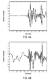
- FIGS 4A-4B show processed waveforms generated from hydrophone and geophone outputs, respectively.
- the waveform recorded by the hydrophone represents the pressure at times following the initial pressure impulse, with the amplitude of the waveform at a point in time related to the pressure wavefield at the hydrophone at the point in time.
- the geophone provides an indication of the fluid particle velocity or acceleration, in a vertical direction, related to the pressure wavefield at the geophone at the point in time.
- Subterranean formations located beneath a volume of water can also be investigated using ocean bottom seismic techniques.
- One example of these techniques is implemented with ocean bottom cables ("OBCs").
- FIG 5 shows an example of an exploration-seismology vessel 502 equipped with two OBCs 504 and 506.
- the OBCs are similar to the towed streamer cables described above in that the OBCs include a number of spaced-apart receivers 508, such as receivers deployed approximately every 25 to 50 meters, but the OBCs are laid on the solid surface 106.
- the OBCs are electronically connected to the anchored recording vessel 502 that provides power, instrument command and control, and data telemetry of the sensor data to the recording equipment on board the vessel.
- ocean bottom seismic techniques can be implemented with autonomous systems composed of receiver nodes that are deployed and recovered using remote operated vehicles.
- the receiver nodes are typically placed on the sea floor in a fairly coarse grid, such as approximately 400 meters apart.
- Autonomous receiver systems are typically implemented using one of two types of receiver node systems.
- a first receiver node system is a cable system in which the receiver nodes are connected by cables to each other and are connected to an anchored recording vessel. The cabled systems have power supplied to each receiver node along a cable and seismic data is returned to the recording vessel along the cable or using radio telemetry.
- a second receiver node system uses self-contained receiver nodes that have a limited power supply, but the receiver nodes typically have to be retrieved in order to download recorded seismic data.
- a separate source vessel equipped with at least one seismic source can be used to generate pressure impulses at spatial and temporal intervals as the source vessel moves across the free surface.
- FIGS 6A-6B show top and side-elevation views, respectively, of an exploration-seismology vessel 602 towing a source 604, and six separate streamers 606-611 located beneath a free surface 612. Each streamer is attached at one end to the vessel 602 and at the opposite end to a buoy, such as buoy 614 attached to the steamer 610.
- the streamers 606-611 form an essentially planar horizontal receiver acquisition surface located beneath the free surface 612.
- the receiver acquisition surface is smoothly varying due to active sea currents and weather conditions.
- the towed streamers may undulate as a result of dynamic conditions of the fluid.
- Figure 6B represents a snapshot, at an instant in time, of the free surface 612 and corresponding smooth wave-like shape in the streamer 609.
- the source 604 can be implemented as an array of seismic source elements, such as air guns and/or water guns, in order to amplify sound waves and overcome undesirable aspects of a signature associated with using a single source element.
- the source 604 may be towed by a separate vessel.
- Figure 6 illustrates use of six streamers 606-611, other embodiments might include additional streamers, including up to as many as 20 or more streamers towed by exploration-seismology vessel 602.
- At least one of the streamers may be towed at a different depth than streamers 606-611, and one or more of the streamers may be towed with a depth profile that is an essentially planar horizontal acquisition surface at an angle to free surface 612.
- Figures 6A and 6B include an xy -plane 616 and an xz -plane 618 of the same Cartesian coordinate system used to specify orientations and coordinate locations within the fluid volume.
- the x coordinate uniquely specifies the position of a point in a direction parallel to the length of the streamers
- the y coordinate uniquely specifies the position of a point in a direction perpendicular to the x axis and substantially parallel to the free surface 612.
- the x -direction is referred to as the "inline” direction
- the y -direction is referred to as the "crossline” direction.
- the z coordinate uniquely specifies the position of a point perpendicular to the xy -plane with the positive z-direction pointing downward away from the free surface 612.
- the streamer 609 is at a depth, z ', below the free surface 612, which can be estimated at various locations along the streamers from depth measuring devices (not shown) attached to the streamers.
- depth measuring devices may measure hydrostatic pressure or utilize acoustic distance measurements.
- the depth measuring devices may be integrated with depth controllers, such as paravanes or water kites.
- the depth measuring devices are typically placed at about 300 meter intervals along each streamer.
- the estimated streamer depths are then used to calculate a two-dimensional interpolated streamer shape that approximates the wave-like shape of an actual streamer at an instant in time.
- the estimated streamer depths can be used to calculate a three-dimensional interpolated surface approximation of the acquisition surface.
- the depth and the elevation of the free-surface profile are estimated with respect to the geoid, which is represented in Figure 6B by dotted line 620.
- shaded disks such as shaded disk 622, represent receivers spaced apart along each streamer. The coordinates of the receivers are denoted by ( x r , y r , z r ) , where the depth z r can be an interpolated value.
- Figure 7 shows a side or xz -plane view of the streamer 609 located beneath the free surface 612.
- Each receiver 622 includes a pressure sensor and three motion sensors.
- Figure 7 includes a magnified view 702 of the receiver 622 that includes a pressure sensor 704 and motion sensors 706.
- the pressure sensors can be hydrophones that measure the pressure wavefield
- the motion sensors can be particle velocity sensors, also called geophones, or particle acceleration sensors, called accelerometers.
- Each pressure sensor measures the total pressure wavefield, denoted by P ( x r , y r , z r , t), in all directions, while the motion sensors of each receiver measure velocity wavefield components of a velocity wavefield vector, denoted by ( V x , V y , V z ) , where V x ( x r , y r , z r , t ), V y ( x r , y r , z r , t ), and V z ( x r , y r , z r , t) are measured velocity wavefields in the x-, y-, and z-directions, respectively, as represented in magnified view 708.
- Figure 8 shows a Cartesian coordinate system with the origin 800 centered at three motion sensors (not shown) of a receiver.
- the velocity wavefield components V x ( x r , y r , z r , t ) 801, V y ( x r , y r , z r , t ) 802, and V z ( x r , y r , z r , t ) 803 are directed along x-, y-, and z -coordinate axes, respectively.
- the motion sensors of each receiver are unidirectional in that each motion sensor only measures one directional component of the velocity wavefield vector 804 that points in the direction the wavefield propagates.
- the vertical velocity component, V z also called the vertical velocity wavefield, of the total wavefield is equal to the total wavefield only for wavefields that propagate vertically.
- ⁇ is the angle of incidence between the direction of the total wavefield and the motion sensor orientation.
- the OBCs and autonomous receiver nodes used in ocean bottom seismic technique also form a receiver acquisition surface.
- the receivers used in ocean bottom seismic techniques can also be implemented with pressure sensors and three motion sensors that measure particle motion in three dimensions, as described above.
- each receiver of an OBC or an autonomous receiver node can be implemented with a pressure sensor that measures the total pressure wavefield P ( x r , y r , z r , t ) and includes three motion sensors that measure velocity wavefield components V x ( x r , y r , z r , t ) , V y ( x r , y r , z r , t ), and V z ( x r , y r , z r , t) in the x-, y-, and z-directions, respectively.
- the receiver acquisition surface spatially samples the wavefield with the receivers separated by a distance ⁇ x in the in-line or x -direction and by a distance ⁇ y in the cross-line or y -direction, as shown in Figure 6A .
- large receiver separation can result in a spatially aliased recorded wavefield.
- the streamers are typically manufactured with the receiver separation distance short enough to avoid aliasing in the inline direction, but when the data acquisition surface is deployed, the streamers are typically separated in the cross-line direction by approximately 50 to 100 meters, which often results in the recorded wavefield being aliased in the cross-line direction.
- Figures 9A-9B show an example of aliasing using sinusoidal wave representations of waves recorded along two different lines of receives at a given instance of time.
- solid circles such as solid circle 902
- a sinusoid dashed-line curve 904 represents a wave, such as a pressure wave or a velocity wave, at an instant in time.
- Open circles, such as open circle 906, represent the amplitude of the wave 904 recorded by the receivers at the instant of time.
- the receivers are separated by a distance ⁇
- the receives are separated by a larger distance ⁇ ' (i.e., ⁇ '> ⁇ ).
- the receivers are spaced close enough to avoid spatial aliasing, because with the receivers separated by the distance ⁇ , the wave 904 can be reconstructed from the amplitudes recorded by the receivers.
- the receivers are spaced so that spatial aliasing cannot be avoided.
- Solid-line curve 908 represents a curve that is hypothetically reconstructed from the recorded amplitudes measured by the receivers. Because the receivers are spaced far apart, the reconstructed wave 908 has a much larger wavelength ⁇ ' than the actual wavelength ⁇ of the original wave 904. Thus, the receivers of Figure 9B cannot be used to reliably reconstruct the original wave 904.
- the Nyquist wavenumber corresponds to the maximum number of cycles per meter that can be accurately recovered by sequential observation. Spatial aliasing occurs when a wave has more cycles per meter than k N . In other words, spatial aliasing occurs when the wavenumber k associated with a wavefield is greater than the Nyquist wavenumber k N (i.e., k > k N or ⁇ ⁇ ⁇ N ). Receiver spacing ⁇ that is less than ⁇ N /2 ensures that the actual wavefield can be reconstructed from the measured wavefield.
- the pressure wavefield P and the vertical velocity wavefield V z can be decomposed into an up-going wavefield and a down-going wavefield.
- Equations (6) The up-going and down-going pressure and velocity wavefields represented in Equations (6) can be rewritten in terms of the measured horizontal velocity wavefield components V x and V y in order to avoid determination of the incidence angle ⁇ as follows.
- V z ⁇ V ⁇ ⁇ cos ⁇ where
- is the absolute value or modulus of a complex number; and ⁇ V ⁇ ⁇ V x 2 + V y 2 + V z 2 where
- Equations (6) and (10) Equations (6)
- V z d 1 2 ⁇ V z + V z Z ⁇ V ⁇ ⁇ ⁇ P
- the scaling factor can be further reduced to a function of solely the horizontal velocity wavefields V x and V y and the pressure wavefield P using principles of ray theory.
- wavefield separation is not compromised by the overlap between up-going and down-going wavefield signals up to the highest incidence angles
- Figure 10 shows a Cartesian coordinate system with the origin 1000 centered at three motion sensors of a receiver (not shown).
- the slowness vector 1002 components p x ( x r , y r , z r , t ) 1003, p y ( x r , y r , z r , t ) 1004, and p z ( x r , y r , z r , t ) 1005 are directed along x -, y-, and z -coordinate axes.
- the slowness vector has the same polar angle ⁇ with respect to the z -axis as the velocity vector has with the z -axis shown in Figure 8 .
- the component of the slowness vector in the z-direction, p z can be rewritten as a function of the x- and y -horizontal velocity wavefields and the pressure wavefield as follows:
- p z 1 c 2 - ⁇ 2 ⁇ V x 2 P 2 - ⁇ 2 ⁇ V y 2 P 2
- Equations (19) are computed for all angles locally in the space-time domain without using information from neighboring traces.
- the result of this single trace approach is that wavefield separation is not influenced by spatial sampling and wavefield separation is not affected by spatial aliasing.
- the signals of a trace can be extrapolated beyond spatial aliasing. For example, by ray tracing either upwards or downward from an initial position at a separation level to a final position at an arbitrary depth level the signals of a trace can be extrapolated beyond aliasing.
- the up-going wavefield is extrapolated upwards forward in time and downwards backward in time.
- the signals of a down-going wavefield are extrapolated upwards backward in time and downwards forward in time.
- the wavefield separation can be performed in the wavenumber-frequency domain by applying a transform, such as a Fourier transform, to the measured velocity wavefields V x , V y , and V z and the pressure wavefield P prior to insertion into equations for the up-going and down-going wavefields presented above in Equations (19).
- a transform such as a Fourier transform
- the measured velocity wavefields V x , V y , and V z and the pressure wavefield P can be transformed using a Fourier transform: V x x r ⁇ y r ⁇ z r ⁇ t ⁇ ⁇ FT ⁇ V ⁇ x k x ⁇ k y ⁇ z r ⁇ ⁇ , V y x r ⁇ y r ⁇ z r ⁇ t ⁇ FT ⁇ V ⁇ y k x ⁇ k y ⁇ z r ⁇ , V z x r ⁇ y r ⁇ z r ⁇ t ⁇ FT ⁇ V ⁇ z k x ⁇ k y ⁇ z r ⁇ , and P x r ⁇ y r ⁇ z r ⁇ t ⁇ FT ⁇ P ⁇ k x ⁇ k ⁇ k ⁇ y ⁇ z
- the Fourier transform can be executed as a discrete Fast Fourier transform ("DFFT") for speed and computational efficiency.
- the calculation of up-going and down-going wavefields using the transformed measured velocity wavefields ⁇ x , ⁇ y , and ⁇ z and the pressure wavefield P in the wavenumber-frequency domain is given by:
- P ⁇ u 1 2 ⁇ P ⁇ - Z 1 - Z 2 ⁇ V ⁇ x 2 P ⁇ 2 - Z 2 ⁇ V ⁇ y 2 P ⁇ 2 ⁇ V ⁇ z
- P ⁇ d 1 2 ⁇ P ⁇ + Z 1 - Z 2 ⁇ V ⁇ x 2 P ⁇ 2 - Z 2 ⁇ V ⁇ y 2 P ⁇ 2
- Equations (23) uses the amplitude ratios (i.e., spectral ratios) of the horizontal velocity wavefields and the pressure wavefield for scaling in contrast to other techniques, where the frequency and wavenumber values are directly used from the frequency-wavenumber domain. Because the spectral ratios in Equations (23) are not affected by aliasing, the separation method described above works accurately beyond aliasing.
- the original up-going and down-going wavefields in the space-time domain can be recovered by applying an inverse transform to the up-going and down-going wavefields in the wavenumber-frequency domain: P ⁇ u k x ⁇ k y ⁇ z r ⁇ ⁇ ⁇ ⁇ IFT ⁇ P u x r ⁇ y r ⁇ z r ⁇ t , P ⁇ d k x ⁇ k y ⁇ z r ⁇ ⁇ ⁇ IFT ⁇ P d x r ⁇ y r ⁇ z r ⁇ t , V ⁇ z u k x ⁇ k y ⁇ z r ⁇ ⁇ ⁇ IFT ⁇ V z u x ⁇ k y ⁇ z r ⁇ ⁇ ⁇ IFT ⁇ V z u x r ⁇ y r ⁇ z r ⁇ t , and V
- Wavefield principles can also be used with wavefield extrapolation in the wavenumber-frequency domain.
- a detailed description including a synthetic data example is presented below.
- ⁇ represents the up-going wavefields P ⁇ u and V ⁇ z u
- D represents the down-going wavefields P ⁇ d and V ⁇ z d in the wavenumber-frequency
- Figure 11 shows an xz -plane example representation of wavefield extrapolation from a depth z below a free surface, where W represents the up-going or down-going wavefield.
- Directional arrow 1102 represents the x -axis
- directional arrow 1104 represents the z -axis
- curve 1106 represents the free surface.
- dashed line 1108 represents a depth of z below the free surface 1106.
- Equations (25) present wavefield extrapolation as multiplying the wavefield in the wavenumber-frequency domain by exponentials that are functions of the vertical component of the slowness vector, p ⁇ z .
- Spatial Aliasing aliasing can be avoided the in-line and cross-line directions when the receivers are spaced so that k x ⁇ k N and k y ⁇
- Figure 12 shows an example plot of the angular frequency ⁇ as a function of the horizontal wavenumber k x .
- Directional arrow 1201 is the horizontal wavenumber k x axis
- directional arrow 1202 is the angular frequency ⁇ axis.
- Line 1203 represents alias-free plane wave contributions to the angular frequency ⁇ as a function of the horizontal wavenumber k x .
- Alias-free plane waves have an angular frequency ⁇ equal to zero when the associated wavenumber k x is zero.
- line 1204 represents aliased plane wave contributions to the angular frequency ⁇ as a function of the horizontal wavenumber k x .
- Points along the line 1204, such as point 1206, represent plane waves associated with spatial aliasing and are incorrectly mapped, or folded back, from wavenumbers k x > k N .
- extrapolation of a wavefield using Equations (25)-(28) is disrupted when the wavefields is spatial aliased in at least one of the horizontal directions.
- Equations (25)-(28) cannot be used to calculate an accurate image a subterranean formation, because the calculated vertical component p ⁇ z is disrupted by spatial aliasing associated with one or both of the horizontal components p ⁇ x and p ⁇ y .
- the equations of motion are independent of position in the wavenumber-frequency domain for any values of the wavenumbers
- Equations (29) enable computation of the horizontal slowness vector components p ⁇ x and p ⁇ y without disruptions due to spatial aliasing.
- numerical stabilization may be used in calculations that involve wavefield amplitude ratios.
- the multiplicative factors A 1 , A 2 , A 3 , and A 4 in Equations (31) and (32) are introduced to account for amplitude changes due to extrapolation.
- the horizontal slowness vector components p x and p y can be calculated from the measured horizontal velocity wavefields and the measured pressure wavefields, the computational complications due to spatial aliasing are avoided. Numerical stabilization may also be used in calculations that involve wavefield amplitude ratios in time domain.
- Figure 13A shows a flow diagram of a method for extrapolating a wavefield in the wavenumber-frequency domain.
- measured pressure wavefield P and measured vector velocity wavefield ( V x , V y , V z ) data is received.
- the pressure wavefield can be obtained from pressure sensors that measure the total pressure wavefield in all directions, and the vector velocity wavefield components V x , V y , and V z can be obtained from separate motion sensors that measure the wavefields in the x -, y-, and z-directions, as described above with reference to Figure 6 .
- the pressure wavefield and velocity wavefields are transformed from the space-time domain to the wavenumber-frequency domain to obtain transformed wavefields P, ⁇ x , ⁇ y , and ⁇ z .
- the wavefields can be transformed from the space-time domain to the wavenumber-frequency domain using a fast Fourier transform for computational efficiency and speed, as described above with reference to Equation (21).
- the measured pressure wavefield is decomposed into up-going and down-going wavefields P ⁇ u and P ⁇ d according to Equations (23a-b).
- the measured vertical velocity wavefield is decomposed into the up-going and down-going vertical velocity wavefields ⁇ u and ⁇ d according to Equations (23c-d). Note that the order in which the operations of blocks 1303 and 1304 are executed is not limited to block 1303 being executed before execution of the operations of block 1304. Alternatively, the order of the operations in blocks 1303 and 1304 can be reversed or these operations can be performed in parallel.
- the vertical component of the slowness vector, p ⁇ z is calculated as a function of the measured horizontal wavefields and the measured pressure wavefield, as described above with reference to Equation (30).
- an up-going or down-going pressure wavefield is extrapolated in the z-direction using Equations (25-26).
- Figure 13B shows a flow diagram of a method for extrapolating a wavefield locally in the time domain.
- measured pressure wavefield P and measured vector velocity wavefield ( V x , V y , V z ) data is received.
- the pressure wavefield can be obtained from pressure sensors that measure the total pressure wavefield in all directions, and the vector velocity wavefield components V x , V y , and V z can be obtained from separate motion sensors that measure the wavefields in the x -, y-, and z-directions, as described above with reference to Figure 6 .
- the measured pressure wavefield is decomposed into up-going and down-going wavefields P u and P d according to Equations (19a-b).
- the measured vertical velocity wavefield is decomposed into the up-going and down-going vertical velocity wavefields V u and V d according to Equations (19c-d). Note that the order in which the operations of blocks 1312 and 1313 are executed is not limited to block 1312 being executed before execution of the operations of block 1313. Alternatively, the order of the operations in blocks 1312 and 1313 can be reversed or these operations can be performed in parallel.
- the vertical components of the slowness vector, p z , p x , and p y are calculated as functions of the measured horizontal velocity wavefields and the measured pressure wavefield, as described above with reference to Equations (15), (16a), and (16b).
- an up-going or down-going pressure wavefield is extrapolated in the z-direction using Equation (31)-(32).
- Figure 14 shows an example of a generalized computer system that executes an efficient method for extrapolating wavefields while bypassing spatial aliasing and therefore represents a seismic-analysis data-processing system.
- the internal components of many small, mid-sized, and large computer systems as well as specialized processor-based storage systems can be described with respect to this generalized architecture, although each particular system may feature many additional components, subsystems, and similar, parallel systems with architectures similar to this generalized architecture.
- the computer system contains one or multiple central processing units (“CPUs”) 1402-1405, one or more electronic memories 1408 interconnected with the CPUs by a CPU/memory-subsystem bus 1410 or multiple busses, a first bridge 1412 that interconnects the CPU/memory-subsystem bus 1410 with additional busses 1414 and 1416, or other types of high-speed interconnection media, including multiple, high-speed serial interconnects.
- CPUs central processing units
- electronic memories 1408 interconnected with the CPUs by a CPU/memory-subsystem bus 1410 or multiple busses
- a first bridge 1412 that interconnects the CPU/memory-subsystem bus 1410 with additional busses 1414 and 1416, or other types of high-speed interconnection media, including multiple, high-speed serial interconnects.
- the busses or serial interconnections connect the CPUs and memory with specialized processors, such as a graphics processor 1418, and with one or more additional bridges 1420, which are interconnected with high-speed serial links or with multiple controllers 1422-1427, such as controller 1427, that provide access to various different types of computer-readable media, such as computer-readable medium 1428, electronic displays, input devices, and other such components, subcomponents, and computational resources.
- the electronic displays including visual display screen, audio speakers, and other output interfaces
- the input devices including mice, keyboards, touch screens, and other such input interfaces, together constitute input and output interfaces that allow the computer system to interact with human users.
- Computer-readable medium 1428 is a data-storage device, including electronic memory, optical or magnetic disk drive, USB drive, flash memory and other such data-storage device.
- the computer-readable medium 1428 can be used to store machine-readable instructions that encode the computational methods described above and can be used to store encoded data, during store operations, and from which encoded data can be retrieved, during read operations, by computer systems, data-storage systems, and peripheral devices.
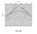
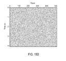
- Figures 15A-15G show plots of modeled and calculated pressure wavefields versus time.
- Figure 15A shows total pressure wavefield data that was generated using the reflectivity modeling method, which represents the data measured by a hydrophone.
- Figure 15B shows the up-going pressure wavefield obtained from Equation (21a).
- Figure 15C shows a modeled up-going pressure wavefield.
- Figure 15D shows the difference between the calculated using the Equation (21a) and the ideal case presented in Figure 15C .
- Figure 15D reveals that the up-going pressure wavefield calculated from Equation (21a) is a very good approximation to the reflectivity modeled up-going pressure wavefield shown in Figure 15C because much of Figure 15D is blank.
- Figures 15E-15G show the effect of wavefield separation and extrapolation.
- Figure 15E shows the up-going pressure wavefield represented in Figure 15B after forward extrapolation by 15 meters upwards to the free surface, multiplication by -1 (the free surface reflection coefficient), and extrapolation downward to 15 meters again.
- the wavefield shown in Figure 15E resulting in a down-going wavefield at the receiver level that was added to the modeled (ideal) up-going wavefield shown in Figure 15A to give the total pressure wavefield shown in Figure 14F .
- Figure 15G shows the error of separation and extrapolation that resulted from subtraction of wavefield shown in Figure 15F from the modeled total pressure field shown in Figure 15A .
- any number of different computational-processing-method implementations that carry out efficient wavefield extrapolation using horizontal slowness vector components that depend on measured horizontal velocity wavefields and measured pressured wavefields may be designed and developed using various different programming languages and computer platforms and by varying different implementation parameters, including control structures, variables, data structures, modular organization, and other such parameters.
- the computational representations of wavefields, operators, and other computational objects may be implemented in different ways.
Landscapes
- Life Sciences & Earth Sciences (AREA)
- Physics & Mathematics (AREA)
- Remote Sensing (AREA)
- Engineering & Computer Science (AREA)
- Geology (AREA)
- Environmental & Geological Engineering (AREA)
- Acoustics & Sound (AREA)
- General Life Sciences & Earth Sciences (AREA)
- General Physics & Mathematics (AREA)
- Geophysics (AREA)
- Oceanography (AREA)
- Geophysics And Detection Of Objects (AREA)
- Measuring Fluid Pressure (AREA)
Applications Claiming Priority (1)
| Application Number | Priority Date | Filing Date | Title |
|---|---|---|---|
| US13/680,287 US10459097B2 (en) | 2012-11-19 | 2012-11-19 | Methods and systems for extrapolating wavefields |
Publications (2)
| Publication Number | Publication Date |
|---|---|
| EP2733508A1 true EP2733508A1 (fr) | 2014-05-21 |
| EP2733508B1 EP2733508B1 (fr) | 2021-07-28 |
Family
ID=49674137
Family Applications (1)
| Application Number | Title | Priority Date | Filing Date |
|---|---|---|---|
| EP13192707.1A Active EP2733508B1 (fr) | 2012-11-19 | 2013-11-13 | Procédés et systèmes pour extrapoler des champs d'ondes |
Country Status (6)
| Country | Link |
|---|---|
| US (1) | US10459097B2 (fr) |
| EP (1) | EP2733508B1 (fr) |
| AU (1) | AU2013248195B2 (fr) |
| BR (1) | BR102013029371A2 (fr) |
| MX (1) | MX336883B (fr) |
| SG (1) | SG2013079975A (fr) |
Cited By (1)
| Publication number | Priority date | Publication date | Assignee | Title |
|---|---|---|---|---|
| WO2020156748A1 (fr) * | 2019-02-01 | 2020-08-06 | Fraunhofer-Gesellschaft zur Förderung der angewandten Forschung e.V. | Système, procédé et module de traitement permettant de détecter un ou de plusieurs objets au fond de la mer |
Families Citing this family (10)
| Publication number | Priority date | Publication date | Assignee | Title |
|---|---|---|---|---|
| US8547786B2 (en) * | 2007-06-29 | 2013-10-01 | Westerngeco L.L.C. | Estimating and using slowness vector attributes in connection with a multi-component seismic gather |
| SG11201610570VA (en) | 2014-07-01 | 2017-01-27 | Pgs Geophysical As | Wavefield reconstruction |
| US10393901B2 (en) | 2015-08-31 | 2019-08-27 | Pgs Geophysical As | Wavefield interpolation and regularization in imaging of multiple reflection energy |
| EP3359982B1 (fr) * | 2015-10-07 | 2022-12-14 | Services Pétroliers Schlumberger | Orientation de capteur sismique |
| US20190206068A1 (en) * | 2016-10-04 | 2019-07-04 | Halliburton Energy Services, Inc. | Monitoring a subterranean formation using motion data |
| US20190101662A1 (en) * | 2017-10-04 | 2019-04-04 | Westerngeco Llc | Compressive sensing marine streamer system |
| WO2019222809A1 (fr) | 2018-05-23 | 2019-11-28 | Woodside Energy Technologies Pty Ltd | Système et procédé d'acquisition de données autonomes |
| US11035970B2 (en) | 2019-06-19 | 2021-06-15 | Magseis Ff Llc | Interleaved marine diffraction survey |
| CN112764098B (zh) * | 2019-11-04 | 2024-09-27 | 中国石油天然气集团有限公司 | 波场分析系统及方法 |
| GB2605108B (en) * | 2019-12-20 | 2024-02-21 | Dug Tech Australia Pty Ltd | Deconvolution of down-going seismic wavefields |
Citations (5)
| Publication number | Priority date | Publication date | Assignee | Title |
|---|---|---|---|---|
| US20040223411A1 (en) * | 2003-01-15 | 2004-11-11 | Westerngeco L.L.C. | Method for retrieving local near-surface material information |
| US20080089174A1 (en) * | 2006-10-11 | 2008-04-17 | Walter Sollner | Method for attenuating particle motion sensor noise in dual sensor towed marine seismic streamers |
| US20090003132A1 (en) * | 2007-06-29 | 2009-01-01 | Massimiliano Vassallo | Estimating and Using Slowness Vector Attributes in Connection with a Multi-Component Seismic Gather |
| US20100091610A1 (en) * | 2008-10-14 | 2010-04-15 | Walter Sollner | Method for imaging a sea-surface reflector from towed dual-sensor streamer data |
| US20110242937A1 (en) * | 2010-03-30 | 2011-10-06 | Soellner Walter | Method for separating up and down propagating pressure and vertical velocity fields from pressure and three-axial motion sensors in towed streamers |
Family Cites Families (1)
| Publication number | Priority date | Publication date | Assignee | Title |
|---|---|---|---|---|
| US7646672B2 (en) * | 2008-01-18 | 2010-01-12 | Pgs Geophysical As | Method for wavefield separation in 3D dual sensor towed streamer data with aliased energy in cross-streamer direction |
-
2012
- 2012-11-19 US US13/680,287 patent/US10459097B2/en active Active
-
2013
- 2013-10-23 SG SG2013079975A patent/SG2013079975A/en unknown
- 2013-10-23 AU AU2013248195A patent/AU2013248195B2/en active Active
- 2013-11-13 EP EP13192707.1A patent/EP2733508B1/fr active Active
- 2013-11-14 BR BR102013029371-7A patent/BR102013029371A2/pt not_active Application Discontinuation
- 2013-11-19 MX MX2013013521A patent/MX336883B/es active IP Right Grant
Patent Citations (5)
| Publication number | Priority date | Publication date | Assignee | Title |
|---|---|---|---|---|
| US20040223411A1 (en) * | 2003-01-15 | 2004-11-11 | Westerngeco L.L.C. | Method for retrieving local near-surface material information |
| US20080089174A1 (en) * | 2006-10-11 | 2008-04-17 | Walter Sollner | Method for attenuating particle motion sensor noise in dual sensor towed marine seismic streamers |
| US20090003132A1 (en) * | 2007-06-29 | 2009-01-01 | Massimiliano Vassallo | Estimating and Using Slowness Vector Attributes in Connection with a Multi-Component Seismic Gather |
| US20100091610A1 (en) * | 2008-10-14 | 2010-04-15 | Walter Sollner | Method for imaging a sea-surface reflector from towed dual-sensor streamer data |
| US20110242937A1 (en) * | 2010-03-30 | 2011-10-06 | Soellner Walter | Method for separating up and down propagating pressure and vertical velocity fields from pressure and three-axial motion sensors in towed streamers |
Cited By (2)
| Publication number | Priority date | Publication date | Assignee | Title |
|---|---|---|---|---|
| WO2020156748A1 (fr) * | 2019-02-01 | 2020-08-06 | Fraunhofer-Gesellschaft zur Förderung der angewandten Forschung e.V. | Système, procédé et module de traitement permettant de détecter un ou de plusieurs objets au fond de la mer |
| US11796701B2 (en) | 2019-02-01 | 2023-10-24 | Fraunhofer-Gesellschaft Zur Foerderung Der Angewandten Forschung E.V. | System, method, and processing module for detecting one or more objects in the seabed |
Also Published As
| Publication number | Publication date |
|---|---|
| US20140140171A1 (en) | 2014-05-22 |
| BR102013029371A2 (pt) | 2014-10-07 |
| AU2013248195A1 (en) | 2014-06-05 |
| MX2013013521A (es) | 2014-05-22 |
| EP2733508B1 (fr) | 2021-07-28 |
| SG2013079975A (en) | 2014-06-27 |
| US10459097B2 (en) | 2019-10-29 |
| AU2013248195B2 (en) | 2017-06-08 |
| MX336883B (es) | 2016-02-03 |
Similar Documents
| Publication | Publication Date | Title |
|---|---|---|
| EP2733508B1 (fr) | Procédés et systèmes pour extrapoler des champs d'ondes | |
| US11327196B2 (en) | Marine surveys conducted with multiple source arrays | |
| US11428834B2 (en) | Processes and systems for generating a high-resolution velocity model of a subterranean formation using iterative full-waveform inversion | |
| US9279898B2 (en) | Methods and systems for correction of streamer-depth bias in marine seismic surveys | |
| EP4042210B1 (fr) | Détermination des propriétés d'une formation souterraine à l'aide d'une équation d'onde acoustique ayant un paramétrage de réflectivité | |
| US9442209B2 (en) | Methods and systems for reconstruction of low frequency particle velocity wavefields and deghosting of seismic streamer data | |
| US9291737B2 (en) | Methods and systems for imaging subterranean formations with primary and multiple reflections | |
| US9857490B2 (en) | Methods and systems for optimizing generation of seismic images | |
| AU2015261556B2 (en) | Wavefield separation based on a matching operator between sensor responses in multi-component streamers | |
| EP3136130B1 (fr) | Régularisation et interpolation de champ d'onde dans l'imagerie d'énergie de réflexion multiple | |
| AU2013201070B2 (en) | Methods and systems for deghosting marine seismic wavefields using cost-functional minimization | |
| US9829593B2 (en) | Determination of an impulse response at a subsurface image level | |
| US20230305176A1 (en) | Determining properties of a subterranean formation using an acoustic wave equation with a reflectivity parameterization |
Legal Events
| Date | Code | Title | Description |
|---|---|---|---|
| PUAI | Public reference made under article 153(3) epc to a published international application that has entered the european phase |
Free format text: ORIGINAL CODE: 0009012 |
|
| 17P | Request for examination filed |
Effective date: 20131113 |
|
| AK | Designated contracting states |
Kind code of ref document: A1 Designated state(s): AL AT BE BG CH CY CZ DE DK EE ES FI FR GB GR HR HU IE IS IT LI LT LU LV MC MK MT NL NO PL PT RO RS SE SI SK SM TR |
|
| AX | Request for extension of the european patent |
Extension state: BA ME |
|
| R17P | Request for examination filed (corrected) |
Effective date: 20141121 |
|
| RBV | Designated contracting states (corrected) |
Designated state(s): AL AT BE BG CH CY CZ DE DK EE ES FI FR GB GR HR HU IE IS IT LI LT LU LV MC MK MT NL NO PL PT RO RS SE SI SK SM TR |
|
| STAA | Information on the status of an ep patent application or granted ep patent |
Free format text: STATUS: EXAMINATION IS IN PROGRESS |
|
| 17Q | First examination report despatched |
Effective date: 20190221 |
|
| STAA | Information on the status of an ep patent application or granted ep patent |
Free format text: STATUS: EXAMINATION IS IN PROGRESS |
|
| GRAP | Despatch of communication of intention to grant a patent |
Free format text: ORIGINAL CODE: EPIDOSNIGR1 |
|
| STAA | Information on the status of an ep patent application or granted ep patent |
Free format text: STATUS: GRANT OF PATENT IS INTENDED |
|
| INTG | Intention to grant announced |
Effective date: 20210223 |
|
| GRAS | Grant fee paid |
Free format text: ORIGINAL CODE: EPIDOSNIGR3 |
|
| GRAA | (expected) grant |
Free format text: ORIGINAL CODE: 0009210 |
|
| STAA | Information on the status of an ep patent application or granted ep patent |
Free format text: STATUS: THE PATENT HAS BEEN GRANTED |
|
| AK | Designated contracting states |
Kind code of ref document: B1 Designated state(s): AL AT BE BG CH CY CZ DE DK EE ES FI FR GB GR HR HU IE IS IT LI LT LU LV MC MK MT NL NO PL PT RO RS SE SI SK SM TR |
|
| REG | Reference to a national code |
Ref country code: GB Ref legal event code: FG4D |
|
| REG | Reference to a national code |
Ref country code: CH Ref legal event code: EP |
|
| REG | Reference to a national code |
Ref country code: DE Ref legal event code: R096 Ref document number: 602013078516 Country of ref document: DE |
|
| REG | Reference to a national code |
Ref country code: AT Ref legal event code: REF Ref document number: 1415197 Country of ref document: AT Kind code of ref document: T Effective date: 20210815 |
|
| REG | Reference to a national code |
Ref country code: IE Ref legal event code: FG4D |
|
| REG | Reference to a national code |
Ref country code: NO Ref legal event code: T2 Effective date: 20210728 |
|
| REG | Reference to a national code |
Ref country code: LT Ref legal event code: MG9D |
|
| REG | Reference to a national code |
Ref country code: NL Ref legal event code: MP Effective date: 20210728 |
|
| REG | Reference to a national code |
Ref country code: AT Ref legal event code: MK05 Ref document number: 1415197 Country of ref document: AT Kind code of ref document: T Effective date: 20210728 |
|
| PG25 | Lapsed in a contracting state [announced via postgrant information from national office to epo] |
Ref country code: HR Free format text: LAPSE BECAUSE OF FAILURE TO SUBMIT A TRANSLATION OF THE DESCRIPTION OR TO PAY THE FEE WITHIN THE PRESCRIBED TIME-LIMIT Effective date: 20210728 Ref country code: SE Free format text: LAPSE BECAUSE OF FAILURE TO SUBMIT A TRANSLATION OF THE DESCRIPTION OR TO PAY THE FEE WITHIN THE PRESCRIBED TIME-LIMIT Effective date: 20210728 Ref country code: AT Free format text: LAPSE BECAUSE OF FAILURE TO SUBMIT A TRANSLATION OF THE DESCRIPTION OR TO PAY THE FEE WITHIN THE PRESCRIBED TIME-LIMIT Effective date: 20210728 Ref country code: BG Free format text: LAPSE BECAUSE OF FAILURE TO SUBMIT A TRANSLATION OF THE DESCRIPTION OR TO PAY THE FEE WITHIN THE PRESCRIBED TIME-LIMIT Effective date: 20211028 Ref country code: LT Free format text: LAPSE BECAUSE OF FAILURE TO SUBMIT A TRANSLATION OF THE DESCRIPTION OR TO PAY THE FEE WITHIN THE PRESCRIBED TIME-LIMIT Effective date: 20210728 Ref country code: PT Free format text: LAPSE BECAUSE OF FAILURE TO SUBMIT A TRANSLATION OF THE DESCRIPTION OR TO PAY THE FEE WITHIN THE PRESCRIBED TIME-LIMIT Effective date: 20211129 Ref country code: NL Free format text: LAPSE BECAUSE OF FAILURE TO SUBMIT A TRANSLATION OF THE DESCRIPTION OR TO PAY THE FEE WITHIN THE PRESCRIBED TIME-LIMIT Effective date: 20210728 Ref country code: RS Free format text: LAPSE BECAUSE OF FAILURE TO SUBMIT A TRANSLATION OF THE DESCRIPTION OR TO PAY THE FEE WITHIN THE PRESCRIBED TIME-LIMIT Effective date: 20210728 Ref country code: ES Free format text: LAPSE BECAUSE OF FAILURE TO SUBMIT A TRANSLATION OF THE DESCRIPTION OR TO PAY THE FEE WITHIN THE PRESCRIBED TIME-LIMIT Effective date: 20210728 Ref country code: FI Free format text: LAPSE BECAUSE OF FAILURE TO SUBMIT A TRANSLATION OF THE DESCRIPTION OR TO PAY THE FEE WITHIN THE PRESCRIBED TIME-LIMIT Effective date: 20210728 |
|
| PG25 | Lapsed in a contracting state [announced via postgrant information from national office to epo] |
Ref country code: PL Free format text: LAPSE BECAUSE OF FAILURE TO SUBMIT A TRANSLATION OF THE DESCRIPTION OR TO PAY THE FEE WITHIN THE PRESCRIBED TIME-LIMIT Effective date: 20210728 Ref country code: LV Free format text: LAPSE BECAUSE OF FAILURE TO SUBMIT A TRANSLATION OF THE DESCRIPTION OR TO PAY THE FEE WITHIN THE PRESCRIBED TIME-LIMIT Effective date: 20210728 Ref country code: GR Free format text: LAPSE BECAUSE OF FAILURE TO SUBMIT A TRANSLATION OF THE DESCRIPTION OR TO PAY THE FEE WITHIN THE PRESCRIBED TIME-LIMIT Effective date: 20211029 |
|
| PG25 | Lapsed in a contracting state [announced via postgrant information from national office to epo] |
Ref country code: DK Free format text: LAPSE BECAUSE OF FAILURE TO SUBMIT A TRANSLATION OF THE DESCRIPTION OR TO PAY THE FEE WITHIN THE PRESCRIBED TIME-LIMIT Effective date: 20210728 |
|
| REG | Reference to a national code |
Ref country code: DE Ref legal event code: R097 Ref document number: 602013078516 Country of ref document: DE |
|
| PG25 | Lapsed in a contracting state [announced via postgrant information from national office to epo] |
Ref country code: SM Free format text: LAPSE BECAUSE OF FAILURE TO SUBMIT A TRANSLATION OF THE DESCRIPTION OR TO PAY THE FEE WITHIN THE PRESCRIBED TIME-LIMIT Effective date: 20210728 Ref country code: SK Free format text: LAPSE BECAUSE OF FAILURE TO SUBMIT A TRANSLATION OF THE DESCRIPTION OR TO PAY THE FEE WITHIN THE PRESCRIBED TIME-LIMIT Effective date: 20210728 Ref country code: RO Free format text: LAPSE BECAUSE OF FAILURE TO SUBMIT A TRANSLATION OF THE DESCRIPTION OR TO PAY THE FEE WITHIN THE PRESCRIBED TIME-LIMIT Effective date: 20210728 Ref country code: EE Free format text: LAPSE BECAUSE OF FAILURE TO SUBMIT A TRANSLATION OF THE DESCRIPTION OR TO PAY THE FEE WITHIN THE PRESCRIBED TIME-LIMIT Effective date: 20210728 Ref country code: CZ Free format text: LAPSE BECAUSE OF FAILURE TO SUBMIT A TRANSLATION OF THE DESCRIPTION OR TO PAY THE FEE WITHIN THE PRESCRIBED TIME-LIMIT Effective date: 20210728 Ref country code: AL Free format text: LAPSE BECAUSE OF FAILURE TO SUBMIT A TRANSLATION OF THE DESCRIPTION OR TO PAY THE FEE WITHIN THE PRESCRIBED TIME-LIMIT Effective date: 20210728 |
|
| REG | Reference to a national code |
Ref country code: DE Ref legal event code: R119 Ref document number: 602013078516 Country of ref document: DE |
|
| PLBE | No opposition filed within time limit |
Free format text: ORIGINAL CODE: 0009261 |
|
| STAA | Information on the status of an ep patent application or granted ep patent |
Free format text: STATUS: NO OPPOSITION FILED WITHIN TIME LIMIT |
|
| PG25 | Lapsed in a contracting state [announced via postgrant information from national office to epo] |
Ref country code: MC Free format text: LAPSE BECAUSE OF FAILURE TO SUBMIT A TRANSLATION OF THE DESCRIPTION OR TO PAY THE FEE WITHIN THE PRESCRIBED TIME-LIMIT Effective date: 20210728 |
|
| REG | Reference to a national code |
Ref country code: CH Ref legal event code: PL |
|
| 26N | No opposition filed |
Effective date: 20220429 |
|
| PG25 | Lapsed in a contracting state [announced via postgrant information from national office to epo] |
Ref country code: LU Free format text: LAPSE BECAUSE OF NON-PAYMENT OF DUE FEES Effective date: 20211113 Ref country code: IT Free format text: LAPSE BECAUSE OF FAILURE TO SUBMIT A TRANSLATION OF THE DESCRIPTION OR TO PAY THE FEE WITHIN THE PRESCRIBED TIME-LIMIT Effective date: 20210728 Ref country code: BE Free format text: LAPSE BECAUSE OF NON-PAYMENT OF DUE FEES Effective date: 20211130 |
|
| REG | Reference to a national code |
Ref country code: BE Ref legal event code: MM Effective date: 20211130 |
|
| PG25 | Lapsed in a contracting state [announced via postgrant information from national office to epo] |
Ref country code: LI Free format text: LAPSE BECAUSE OF NON-PAYMENT OF DUE FEES Effective date: 20211130 Ref country code: CH Free format text: LAPSE BECAUSE OF NON-PAYMENT OF DUE FEES Effective date: 20211130 |
|
| PG25 | Lapsed in a contracting state [announced via postgrant information from national office to epo] |
Ref country code: IE Free format text: LAPSE BECAUSE OF NON-PAYMENT OF DUE FEES Effective date: 20211113 Ref country code: DE Free format text: LAPSE BECAUSE OF NON-PAYMENT OF DUE FEES Effective date: 20220601 |
|
| PG25 | Lapsed in a contracting state [announced via postgrant information from national office to epo] |
Ref country code: FR Free format text: LAPSE BECAUSE OF NON-PAYMENT OF DUE FEES Effective date: 20211130 |
|
| PG25 | Lapsed in a contracting state [announced via postgrant information from national office to epo] |
Ref country code: HU Free format text: LAPSE BECAUSE OF FAILURE TO SUBMIT A TRANSLATION OF THE DESCRIPTION OR TO PAY THE FEE WITHIN THE PRESCRIBED TIME-LIMIT; INVALID AB INITIO Effective date: 20131113 |
|
| P01 | Opt-out of the competence of the unified patent court (upc) registered |
Effective date: 20230516 |
|
| PG25 | Lapsed in a contracting state [announced via postgrant information from national office to epo] |
Ref country code: CY Free format text: LAPSE BECAUSE OF FAILURE TO SUBMIT A TRANSLATION OF THE DESCRIPTION OR TO PAY THE FEE WITHIN THE PRESCRIBED TIME-LIMIT Effective date: 20210728 |
|
| PG25 | Lapsed in a contracting state [announced via postgrant information from national office to epo] |
Ref country code: MK Free format text: LAPSE BECAUSE OF FAILURE TO SUBMIT A TRANSLATION OF THE DESCRIPTION OR TO PAY THE FEE WITHIN THE PRESCRIBED TIME-LIMIT Effective date: 20210728 |
|
| PG25 | Lapsed in a contracting state [announced via postgrant information from national office to epo] |
Ref country code: MT Free format text: LAPSE BECAUSE OF FAILURE TO SUBMIT A TRANSLATION OF THE DESCRIPTION OR TO PAY THE FEE WITHIN THE PRESCRIBED TIME-LIMIT Effective date: 20210728 |
|
| PGFP | Annual fee paid to national office [announced via postgrant information from national office to epo] |
Ref country code: NO Payment date: 20241129 Year of fee payment: 12 |
|
| PGFP | Annual fee paid to national office [announced via postgrant information from national office to epo] |
Ref country code: GB Payment date: 20241127 Year of fee payment: 12 |