EP2732315B1 - Interactive display of results obtained from the inversion of logging data - Google Patents
Interactive display of results obtained from the inversion of logging data Download PDFInfo
- Publication number
- EP2732315B1 EP2732315B1 EP12821824.5A EP12821824A EP2732315B1 EP 2732315 B1 EP2732315 B1 EP 2732315B1 EP 12821824 A EP12821824 A EP 12821824A EP 2732315 B1 EP2732315 B1 EP 2732315B1
- Authority
- EP
- European Patent Office
- Prior art keywords
- inversion
- plot
- logging
- cross
- logging data
- Prior art date
- Legal status (The legal status is an assumption and is not a legal conclusion. Google has not performed a legal analysis and makes no representation as to the accuracy of the status listed.)
- Active
Links
Images




Classifications
-
- G—PHYSICS
- G01—MEASURING; TESTING
- G01V—GEOPHYSICS; GRAVITATIONAL MEASUREMENTS; DETECTING MASSES OR OBJECTS; TAGS
- G01V3/00—Electric or magnetic prospecting or detecting; Measuring magnetic field characteristics of the earth, e.g. declination, deviation
- G01V3/38—Processing data, e.g. for analysis, for interpretation, for correction
-
- G—PHYSICS
- G01—MEASURING; TESTING
- G01V—GEOPHYSICS; GRAVITATIONAL MEASUREMENTS; DETECTING MASSES OR OBJECTS; TAGS
- G01V3/00—Electric or magnetic prospecting or detecting; Measuring magnetic field characteristics of the earth, e.g. declination, deviation
- G01V3/18—Electric or magnetic prospecting or detecting; Measuring magnetic field characteristics of the earth, e.g. declination, deviation specially adapted for well-logging
Definitions
- This disclosure relates generally to well logging, and more particularly to the interactive display of results obtained from the inversion of the logging data.
- Logging tools have long been used in wellbores to make, for example, formation evaluation measurements to infer properties of the formations surrounding the borehole and the fluids in the formations.
- Common logging tools include electromagnetic tools, nuclear tools, and nuclear magnetic resonance (NMR) tools, though various other tool types are also used.
- NMR nuclear magnetic resonance
- MWD tools typically provide drilling parameter information such as weight on the bit, torque, temperature, pressure, direction, and inclination.
- LWD tools typically provide formation evaluation measurements such as resistivity, porosity, and NMR distributions.
- MWD and LWD tools often have components common to wireline tools (e.g., transmitting and receiving antennas), but MWD and LWD tools must be constructed to not only endure but to operate in the harsh environment of drilling.
- wireline tools e.g., transmitting and receiving antennas
- MWD and LWD tools must be constructed to not only endure but to operate in the harsh environment of drilling.
- the terms MWD and LWD are often used interchangeably, and the use of either term in this disclosure will be understood to include both the collection of formation and wellbore information, as well as data on movement and placement of the drilling assembly.
- US 2007/168133 A1 relates to a computer-based method for while drilling modeling and visualization of layered subterranean earth formations.
- a histogram characterizing uncertainty of a multilayer model is used to generate a set of color hue values which represent predictions of the formation property for depth values above/below the tool.
- US 2009/198447 A1 relates to a system and method for displaying data associated with subsurface reservoirs. At least one property of a subterranean earth formation while drilling a borehole using probability information from a modeling process is visualized. Probability waveforms are produced that are proportional to an amount of uncertainty or error associated with a boundary estimate at a particular distance from an axis of the borehole. By providing a visual display of the uncertainty, a user can make better geosteering decisions.
- This disclosure relates to a method of producing an interactive display of results obtained from the inversion of logging data according to claim 1 and to a system to estimate subsurface formation properties from logging data according to claim 13.
- An interactive display of results obtained from the inversion of logging data is produced by obtaining and inverting the logging data using a Monte-Carlo inversion.
- An interactive plot having a percentile scale plotted against a location parameter is produced and a particular percentile is selected using the interactive plot.
- a cross-section plot for the particular percentile using the results of the Monte-Carlo inversion is produced.
- the particular percentile can be a curve representing a best-fit solution or a polyline representing selected solutions. Background color/shading can be displayed on the interactive plot to indicate user-defined constraints have been applied.
- Uncertain features can be plotted on a corresponding cross- section display using fading. Clusters of solutions that are substantially equally likely, given the measurements at a particular drill location, can be identified and plotted. A cross-section constructed from the layered models belonging to a particular cluster can be overlaid on another cross-section.
- Figure 1 illustrates a well site system in which various embodiments can be employed.
- the well site can be onshore or offshore.
- a borehole 11 is formed in subsurface formations by rotary drilling in a manner that is well known.
- Some embodiments can also use directional drilling, as will be described hereinafter.
- a drill string 12 is suspended within the borehole 11 and has a bottom hole assembly 100 which includes a drill bit 105 at its lower end.
- the surface system includes platform and derrick assembly 10 positioned over the borehole 11, the assembly 10 including a rotary table 16, kelly 17, hook 18 and rotary swivel 19.
- the drill string 12 is rotated by the rotary table 16, energized by means not shown, which engages the kelly 17 at the upper end of the drill string.
- the drill string 12 is suspended from a hook 18, attached to a traveling block (also not shown), through the kelly 17 and a rotary swivel 19 which permits rotation of the drill string relative to the hook.
- a top drive system could alternatively be used.
- the surface system further includes drilling fluid or mud 26 stored in a pit 27 formed at the well site.
- a pump 29 delivers the drilling fluid 26 to the interior of the drill string 12 via a port in the swivel 19, causing the drilling fluid to flow downwardly through the drill string 12 as indicated by the directional arrow 8.
- the drilling fluid exits the drill string 12 via ports in the drill bit 105, and then circulates upwardly through the annulus region between the outside of the drill string and the wall of the borehole, as indicated by the directional arrows 9.
- the drilling fluid lubricates the drill bit 105 and carries formation cuttings up to the surface as it is returned to the pit 27 for recirculation.
- the bottom hole assembly 100 of the illustrated embodiment includes a logging-while-drilling (LWD) module 120, a measuring-while-drilling (MWD) module 130, a roto-steerable system and motor, and drill bit 105.
- LWD logging-while-drilling
- MWD measuring-while-drilling
- roto-steerable system and motor drill bit 105.
- the LWD module 120 is housed in a special type of drill collar, as is known in the art, and can contain one or a plurality of known types of logging tools. It will also be understood that more than one LWD and/or MWD module can be employed, e.g. as represented at 120A. (References, throughout, to a module at the position of 120 can alternatively mean a module at the position of 120A as well.)
- the LWD module includes capabilities for measuring, processing, and storing information, as well as for communicating with the surface equipment. In the present embodiment, the LWD module includes a resistivity measuring device.
- the MWD module 130 is also housed in a special type of drill collar, as is known in the art, and can contain one or more devices for measuring characteristics of the drill string and drill bit.
- the MWD tool further includes an apparatus (not shown) for generating electrical power to the downhole system. This may typically include a mud turbine generator powered by the flow of the drilling fluid, it being understood that other power and/or battery systems may be employed.
- the MWD module includes one or more of the following types of measuring devices: a weight-on-bit measuring device, a torque measuring device, a vibration measuring device, a shock measuring device, a stick/slip measuring device, a direction measuring device, and an inclination measuring device.
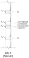
- FIG. 2 An example of a tool which can be the LWD tool 120, or can be a part of an LWD tool suite 120A, is shown in Figure 2 .
- upper and lower transmitting antennas, T 1 and T 2 have upper and lower receiving antennas, R 1 and R 2 , therebetween.
- the antennas are formed in recesses in a modified drill collar and mounted in MC or insulating material.
- the phase shift of electromagnetic energy as between the receivers provides an indication of formation resistivity at a relatively shallow depth of investigation, and the attenuation of electromagnetic energy as between the receivers provides an indication of formation resistivity at a relatively deep depth of investigation.
- U.S. Patent No. 4,899,112 can be referred to for further details.
- attenuation-representative signals and phase-representative signals are coupled to a processor, an output of which is coupleable to a telemetry circuit.
- Recent electromagnetic (EM) logging tools use one or more tilted or transverse antennas, with or without axial antennas.
- Those antennas may be transmitters or receivers.
- a tilted antenna is one whose dipole moment is neither parallel nor perpendicular to the longitudinal axis of the tool.
- a transverse antenna is one whose dipole moment is perpendicular to the longitudinal axis of the tool, and an axial antenna is one whose dipole moment is parallel to the longitudinal axis of the tool.
- a triaxial antenna is one in which three antennas (i.e., antenna coils) are arranged to be mutually orthogonal. Typically, one antenna (coil) is axial and the other two are transverse.
- Two antennas are said to have equal angles if their dipole moment vectors intersect the tool's longitudinal axis at the same angle.
- two tilted antennas have the same tilt angle if their dipole moment vectors, having their tails conceptually fixed to a point on the tool's longitudinal axis, lie on the surface of a right circular cone centered on the tool's longitudinal axis and having its vertex at that reference point.
- Transverse antennas obviously have equal angles of 90 degrees, and that is true regardless of their azimuthal orientations relative to the tool.
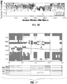
- Figure 3 shows a prior art cross-section display of a 50% quintile formation model generated by a Monte-Carlo inversion.
- the Y-axis of the cross section is typically TVD (True Vertical Depth), and the X-axis is typically THL (True Horizontal Length) in a highly deviated well.
- the X-axis may instead represent a series of tool positions in the case of a vertical or near-vertical well.
- the cross-section display may be a "best" solution, based on some optimization scheme.
- the a posteriori distribution of layered models is displayed as a set of curves alongside (i.e., to the left of) the cross-section.
- Figure 4 shows a similar plot, but one in which an interactive display is placed beneath the X-axis of the cross-section plot.
- a well placement engineer can use such an interactive graphic presentation to more fully exploit the Monte-Carlo inversion results and thereby make geosteering and/or geo-stopping decisions while drilling a well.
- the X-axis of this plot typically represents displacement along the trajectory of a highly-deviated well. It may also represent, for example in a low angle well, a function of displacement, a succession of measurement stations, or a function of a succession of measurement stations. Those parameters are collectively referred to herein as location parameters.
- the Y-axis is a percentile scale representing the a posteriori probability distribution function (PDF) generated by the Monte-Carlo inversion.
- PDF posteriori probability distribution function
- a corresponding curve representing resistivity profile can move synchronously in the vertical resistivity profile plot (top left in Figure 3 ).
- This resistivity profile corresponds to a particular position on the x-axis, typically selected by the user. This provides the user an additional feel for the uncertainty variance versus the depth at a given X-axis position.
- a curve representing the "best solution" from an error minimization point of view can be drawn on the interactive plot. This curve can be selected to generate a cross-section showing the best-fit solution for all x values. Figure 5 shows such a plot.
- Several curves can be displayed simultaneously on the interactive plot, each corresponding to a different selection of Monte-Carlo inversion results.
- the user can select among those curves to move from one cross-section display to another.
- Different methods are available to generate one or several curves in the interactive display, each corresponding to a selection of Monte-Carlo inversion results from which the user can select.
- At least two classes can be distinguished among those methods.
- a first class exploits the outputs of the standard Monte-Carlo inversion.
- One technique from this class decomposes the a posteriori distribution of the Monte-Carlo inversion into the sum of a series of n Gaussian distributions and creates n curves corresponding to the mean of each of those Gaussian distributions.
- a second class introduces additional criteria to select a sub-population of the a posteriori distribution of the standard Monte-Carlo inversion.
- This second class is a direct extension of the Monte-Carlo inversion, where the criteria for a result to be kept not only include the distance between the measured data curves and the curves obtained by a forward modeling of the inversion result, but also include additional conditions such as only those models: having resistivities in a given range at a given distance from the tool, having a given number of beds, belonging to the main cluster of models, yielding local anisotropy in a given range, and having the highest correlation with solutions found at a selected X position.
- An exemplary set of such criteria could be articulated as "results with a local resistivity anisotropy greater than five ohm-m in layers of less than two ohm-m resistivity". One could then compute for each station the best-fit result that satisfies those criteria, thereby defining a curve in the interactive plot and the corresponding cross-section.
- the background of the interactive plot can be colored or shaded as a function of the error, from a minimization point of view, corresponding to the Monte-Carlo inversion result at a particular x station and y percentile.
- the zones over which constraint sets are applied is indicated by the background color (shade) of the percentile display, as shown in Figure 7 .
- No background color (or white background) indicates that the "impartial" Monte-Carlo result is being displayed.
- a further example makes use of a clustering algorithm to provide for an automatic separation of the set of layered models comprising the a posteriori distribution into a set of informative clusters.
- a clustering algorithm to provide for an automatic separation of the set of layered models comprising the a posteriori distribution into a set of informative clusters.
- Figure 8 shows a canvas plot (cross-section) with a resistive layer below the tool that is considered to be an uncertain feature.
- the canvas plot shows the 50th percentile solution, with fading.
- the resistive layer feature below the tool, located below 1020 feet TVD, is an uncertain feature, as the faded out display indicates.
- the user has selected the measurement station in the canvas plot of Figure 8 .
- the corresponding layered model histogram pictured in Figure 9A shows the uncertain resistive feature. In this case, the user has requested an automatic clustering of the set of solutions into two clusters.
- the process of clustering the set of layered models into two clusters can be accomplished as follows.
- I be the true vertical depth interval in which the layered models are defined.
- a matrix D, whose entry D ij is the average horizontal resistivity of the layered model in the i th subinterval is prepared.
- a k-means clustering algorithm to divide the collection of columns of the matrix D (that contain the discretized profiles of resistivity for each layered model) into the user-selected number of clusters, K, is applied.
- the number of clusters K equals two.
- the k-means clustering algorithm returns an index set A that indicates the cluster to which each layered model ⁇ j belongs ( ⁇ j ⁇ ⁇ 1,...,K ⁇ ).
- Figure 9A shows the layered model histograms for the measurement station in the cross-section of Figure 8 .
- Figure 9B shows the subset of solutions designated cluster 1
- Figure 9C shows the subset of solutions designated cluster 2.
- Figure 9A indicates the location of the uncertain resistive feature shown below the tool in Figure 8 . It can be seen from the plots that the median of resistivity in the region above 1010 feet TVD for cluster 1 is more conductive than the median resistivity for cluster 2. Having drilled through the zone above 1010 feet TVD, and knowing the zone is indeed more conductive, the user can select cluster 1 as being more consistent with the local knowledge of the well.
- Figure 10 shows the a posteriori probability of layered models belonging to clusters 1 and 2 from Figure 9 . The graph shows that the two clusters of solutions are largely indistinguishable given the constraints of the measurements.
- An automatic k-means clustering can be performed at the measurement stations near the selected measurement station, and a new curtain plot can be constructed which displays the cluster 1 solutions in the selected region.
- This processing step can be accomplished as follows and shown in Figure 12 .
- Let s s start,..., s end be the indices of the measurement stations for which the user has requested that the k-means clustering be performed.
- Let the index of the selected measurement station where the user has selected the cluster 1 solution be denoted s* and the cluster centroid belonging to the user-selected cluster 1 solution be ⁇ 1,s* .
- the cluster centroid at station s s*+1 with the smallest Euclidean distance to ⁇ 1,s* is identified/labeled (after possibly reordering the clusters and their centroids) ⁇ 1,s*+1 (step 206).
- An entirely similar procedure is conducted (step 210) for the measurement stations to the left of the selected measurement station s ⁇ s*.
- a curtain plot section constructed from the layered models belonging to the cluster 1 solutions can be overlaid on top of the curtain plot from Figure 8 , so the user can inspect the effect of selecting the cluster 1 solutions for this portion of the well.
- Figure 11 is an updated curtain plot display showing the 50th percentile solution without the fading, as well as the cluster 1 solutions selected using the automatic clustering procedure and user prior knowledge.
- the user can partition the Monte Carlo inversion results into clusters of solutions, inspect which cluster is most consistent with the user's knowledge of the field or well, and update the curtain plot section to reflect the user's solution cluster selection.
Landscapes
- Life Sciences & Earth Sciences (AREA)
- Engineering & Computer Science (AREA)
- Environmental & Geological Engineering (AREA)
- Geology (AREA)
- Remote Sensing (AREA)
- Physics & Mathematics (AREA)
- General Life Sciences & Earth Sciences (AREA)
- General Physics & Mathematics (AREA)
- Geophysics (AREA)
- Geophysics And Detection Of Objects (AREA)
Description
- This disclosure relates generally to well logging, and more particularly to the interactive display of results obtained from the inversion of the logging data.
- Logging tools have long been used in wellbores to make, for example, formation evaluation measurements to infer properties of the formations surrounding the borehole and the fluids in the formations. Common logging tools include electromagnetic tools, nuclear tools, and nuclear magnetic resonance (NMR) tools, though various other tool types are also used.
- Early logging tools were run into a wellbore on a wireline cable, after the wellbore had been drilled. Modem versions of such wireline tools are still used extensively. However, the need for information while drilling the borehole gave rise to measurement-while-drilling (MWD) tools and logging-while-drilling (LWD) tools. By collecting and processing such information during the drilling process, the driller can modify or correct key steps of the operation to optimize performance.
- MWD tools typically provide drilling parameter information such as weight on the bit, torque, temperature, pressure, direction, and inclination. LWD tools typically provide formation evaluation measurements such as resistivity, porosity, and NMR distributions. MWD and LWD tools often have components common to wireline tools (e.g., transmitting and receiving antennas), but MWD and LWD tools must be constructed to not only endure but to operate in the harsh environment of drilling. The terms MWD and LWD are often used interchangeably, and the use of either term in this disclosure will be understood to include both the collection of formation and wellbore information, as well as data on movement and placement of the drilling assembly.
-
US 2007/168133 A1 relates to a computer-based method for while drilling modeling and visualization of layered subterranean earth formations. A histogram characterizing uncertainty of a multilayer model is used to generate a set of color hue values which represent predictions of the formation property for depth values above/below the tool. -
US 2009/198447 A1 relates to a system and method for displaying data associated with subsurface reservoirs. At least one property of a subterranean earth formation while drilling a borehole using probability information from a modeling process is visualized. Probability waveforms are produced that are proportional to an amount of uncertainty or error associated with a boundary estimate at a particular distance from an axis of the borehole. By providing a visual display of the uncertainty, a user can make better geosteering decisions. - This disclosure relates to a method of producing an interactive display of results obtained from the inversion of logging data according to
claim 1 and to a system to estimate subsurface formation properties from logging data according to claim 13.
An interactive display of results obtained from the inversion of logging data is produced by obtaining and inverting the logging data using a Monte-Carlo inversion. An interactive plot having a percentile scale plotted against a location parameter is produced and a particular percentile is selected using the interactive plot. A cross-section plot for the particular percentile using the results of the Monte-Carlo inversion is produced. The particular percentile can be a curve representing a best-fit solution or a polyline representing selected solutions. Background color/shading can be displayed on the interactive plot to indicate user-defined constraints have been applied. Uncertain features can be plotted on a corresponding cross- section display using fading. Clusters of solutions that are substantially equally likely, given the measurements at a particular drill location, can be identified and plotted. A cross-section constructed from the layered models belonging to a particular cluster can be overlaid on another cross-section. - Other advantages and features will be apparent from the following detailed description when read in conjunction with the attached drawings.
-
-
Figure 1 illustrates an exemplary well site system. -
Figure 2 shows a prior art electromagnetic logging tool. -
Figure 3 shows a prior art cross-section display of a 50% quintile formation model generated by a Monte-Carlo inversion. -
Figure 4 shows a cross-section display of a selected percentile formation model, but one in which an interactive display is placed beneath the X-axis of the cross-section plot, in accordance with the present disclosure. -
Figure 5 shows a plot of the curve representing the "best solution" from an error minimization point of view drawn on the interactive plot. This curve can be selected to generate a cross-section showing the best-fit solution for all x values, in accordance with the present disclosure. -
Figure 6 shows a plot of a series of points entered by a user to drive the creation of a polyline y = f(x) and to define a cross-section with selected results, in accordance with the present disclosure. -
Figure 7 shows a plot of in which constraints are changed within the inverted interval, the zones over which constraint sets are applied being indicated by the background color (shade) of the percentile display, in accordance with the present disclosure. -
Figure 8 shows a canvas plot (cross-section) with a resistive layer below the tool that is considered to be an uncertain feature, in accordance with the present disclosure. -
Figure 9A shows the layered model histograms for the measurement station indicated by the arrow in the cross-section ofFigure 8 , in accordance with the present disclosure. -
Figure 9B shows the subset of solutions designatedcluster 1, in accordance with the present disclosure. -
Figure 9C shows the subset of solutions designated cluster 2, in accordance with the present disclosure. -
Figure 10 shows the two clusters of solutions fromFigures 9B and 9C are otherwise equally likely given the measurements at the current drill location, in accordance with the present disclosure. -
Figure 11 is a curtain plot display showing the 50th percentile solution without the fading, as well as thecluster 1 solutions selected using the automatic clustering procedure and user prior knowledge, in accordance with the present disclosure. -
Figure 12 shows a flowchart of exemplary steps for an embodiment, in accordance with the present disclosure. - It should be understood that the drawings are not to scale and that the disclosed embodiments are sometimes illustrated diagrammatically and in partial views. In certain instances, details that are not necessary for an understanding of the disclosed method and apparatus or that would render other details difficult to perceive may have been omitted. It should be understood that this disclosure is not limited to the particular embodiments illustrated herein.
- Some embodiments will now be described with reference to the figures. Like elements in the various figures may be referenced with like numbers for consistency. In the following description, numerous details are set forth to provide an understanding of various embodiments and/or features. However, it will be understood by those skilled in the art that some embodiments may be practiced without many of these details and that numerous variations or modifications from the described embodiments are possible. As used here, the terms "above" and "below", "up" and "down", "upper" and "lower", "upwardly" and "downwardly", and other like terms indicating relative positions above or below a given point or element are used in this description to more clearly describe certain embodiments. However, when applied to equipment and methods for use in wells that are deviated or horizontal, such terms may refer to a left to right, right to left, or diagonal relationship, as appropriate.
-
Figure 1 illustrates a well site system in which various embodiments can be employed. The well site can be onshore or offshore. In this exemplary system, aborehole 11 is formed in subsurface formations by rotary drilling in a manner that is well known. Some embodiments can also use directional drilling, as will be described hereinafter. - A drill string 12 is suspended within the
borehole 11 and has abottom hole assembly 100 which includes adrill bit 105 at its lower end. The surface system includes platform andderrick assembly 10 positioned over theborehole 11, theassembly 10 including a rotary table 16, kelly 17, hook 18 and rotary swivel 19. The drill string 12 is rotated by the rotary table 16, energized by means not shown, which engages the kelly 17 at the upper end of the drill string. The drill string 12 is suspended from a hook 18, attached to a traveling block (also not shown), through the kelly 17 and a rotary swivel 19 which permits rotation of the drill string relative to the hook. As is well known, a top drive system could alternatively be used. - In the example of this embodiment, the surface system further includes drilling fluid or
mud 26 stored in a pit 27 formed at the well site. Apump 29 delivers thedrilling fluid 26 to the interior of the drill string 12 via a port in the swivel 19, causing the drilling fluid to flow downwardly through the drill string 12 as indicated by the directional arrow 8. The drilling fluid exits the drill string 12 via ports in thedrill bit 105, and then circulates upwardly through the annulus region between the outside of the drill string and the wall of the borehole, as indicated by the directional arrows 9. In this well known manner, the drilling fluid lubricates thedrill bit 105 and carries formation cuttings up to the surface as it is returned to the pit 27 for recirculation. - The
bottom hole assembly 100 of the illustrated embodiment includes a logging-while-drilling (LWD)module 120, a measuring-while-drilling (MWD) module 130, a roto-steerable system and motor, anddrill bit 105. - The
LWD module 120 is housed in a special type of drill collar, as is known in the art, and can contain one or a plurality of known types of logging tools. It will also be understood that more than one LWD and/or MWD module can be employed, e.g. as represented at 120A. (References, throughout, to a module at the position of 120 can alternatively mean a module at the position of 120A as well.) The LWD module includes capabilities for measuring, processing, and storing information, as well as for communicating with the surface equipment. In the present embodiment, the LWD module includes a resistivity measuring device. - The MWD module 130 is also housed in a special type of drill collar, as is known in the art, and can contain one or more devices for measuring characteristics of the drill string and drill bit. The MWD tool further includes an apparatus (not shown) for generating electrical power to the downhole system. This may typically include a mud turbine generator powered by the flow of the drilling fluid, it being understood that other power and/or battery systems may be employed. In the present embodiment, the MWD module includes one or more of the following types of measuring devices: a weight-on-bit measuring device, a torque measuring device, a vibration measuring device, a shock measuring device, a stick/slip measuring device, a direction measuring device, and an inclination measuring device.
- An example of a tool which can be the
LWD tool 120, or can be a part of an LWD tool suite 120A, is shown inFigure 2 . As seen inFigure 2 , upper and lower transmitting antennas, T1 and T2, have upper and lower receiving antennas, R1 and R2, therebetween. The antennas are formed in recesses in a modified drill collar and mounted in MC or insulating material. The phase shift of electromagnetic energy as between the receivers provides an indication of formation resistivity at a relatively shallow depth of investigation, and the attenuation of electromagnetic energy as between the receivers provides an indication of formation resistivity at a relatively deep depth of investigation.U.S. Patent No. 4,899,112 can be referred to for further details. In operation, attenuation-representative signals and phase-representative signals are coupled to a processor, an output of which is coupleable to a telemetry circuit. - Recent electromagnetic (EM) logging tools use one or more tilted or transverse antennas, with or without axial antennas. Those antennas may be transmitters or receivers. A tilted antenna is one whose dipole moment is neither parallel nor perpendicular to the longitudinal axis of the tool. A transverse antenna is one whose dipole moment is perpendicular to the longitudinal axis of the tool, and an axial antenna is one whose dipole moment is parallel to the longitudinal axis of the tool. A triaxial antenna is one in which three antennas (i.e., antenna coils) are arranged to be mutually orthogonal. Typically, one antenna (coil) is axial and the other two are transverse. Two antennas are said to have equal angles if their dipole moment vectors intersect the tool's longitudinal axis at the same angle. For example, two tilted antennas have the same tilt angle if their dipole moment vectors, having their tails conceptually fixed to a point on the tool's longitudinal axis, lie on the surface of a right circular cone centered on the tool's longitudinal axis and having its vertex at that reference point. Transverse antennas obviously have equal angles of 90 degrees, and that is true regardless of their azimuthal orientations relative to the tool.
-
Figure 3 shows a prior art cross-section display of a 50% quintile formation model generated by a Monte-Carlo inversion. The Y-axis of the cross section is typically TVD (True Vertical Depth), and the X-axis is typically THL (True Horizontal Length) in a highly deviated well. The X-axis may instead represent a series of tool positions in the case of a vertical or near-vertical well. Alternatively, the cross-section display may be a "best" solution, based on some optimization scheme. The a posteriori distribution of layered models is displayed as a set of curves alongside (i.e., to the left of) the cross-section. -
Figure 4 shows a similar plot, but one in which an interactive display is placed beneath the X-axis of the cross-section plot. A well placement engineer can use such an interactive graphic presentation to more fully exploit the Monte-Carlo inversion results and thereby make geosteering and/or geo-stopping decisions while drilling a well. The X-axis of this plot typically represents displacement along the trajectory of a highly-deviated well. It may also represent, for example in a low angle well, a function of displacement, a succession of measurement stations, or a function of a succession of measurement stations. Those parameters are collectively referred to herein as location parameters. The Y-axis is a percentile scale representing the a posteriori probability distribution function (PDF) generated by the Monte-Carlo inversion. - The interactive display is used to control how the results of the Monte-Carlo inversion are used to make the cross-section display. For example, a user can move a horizontal percentile line, using what is referred to herein as the "interactor", to control which results of the Monte-Carlo inversion are used to build the cross-section. Moving the horizontal line from, say, y=50% to y=90% will change the cross-section from representing the median value from an inversion to the 90th percentile results from that inversion for all x values. This may allow the user to better gauge the sensitivity of the results (e.g., the uncertainty in the parameters describing the layered formation). Optionally, when the user changes the percentile in the interactive plot, a corresponding curve representing resistivity profile can move synchronously in the vertical resistivity profile plot (top left in
Figure 3 ). This resistivity profile corresponds to a particular position on the x-axis, typically selected by the user. This provides the user an additional feel for the uncertainty variance versus the depth at a given X-axis position. - A curve representing the "best solution" from an error minimization point of view can be drawn on the interactive plot. This curve can be selected to generate a cross-section showing the best-fit solution for all x values.
Figure 5 shows such a plot. - In another mode of interaction, a series of points can be entered by the user (see
Figure 6 ) to drive the creation of a polyline y = f(x) and to define a cross-section with selected results. Several curves can be displayed simultaneously on the interactive plot, each corresponding to a different selection of Monte-Carlo inversion results. In one interaction mode, the user can select among those curves to move from one cross-section display to another. - Different methods are available to generate one or several curves in the interactive display, each corresponding to a selection of Monte-Carlo inversion results from which the user can select. At least two classes can be distinguished among those methods. A first class exploits the outputs of the standard Monte-Carlo inversion. One technique from this class decomposes the a posteriori distribution of the Monte-Carlo inversion into the sum of a series of n Gaussian distributions and creates n curves corresponding to the mean of each of those Gaussian distributions.
- A second class introduces additional criteria to select a sub-population of the a posteriori distribution of the standard Monte-Carlo inversion. This second class is a direct extension of the Monte-Carlo inversion, where the criteria for a result to be kept not only include the distance between the measured data curves and the curves obtained by a forward modeling of the inversion result, but also include additional conditions such as only those models: having resistivities in a given range at a given distance from the tool, having a given number of beds, belonging to the main cluster of models, yielding local anisotropy in a given range, and having the highest correlation with solutions found at a selected X position. An exemplary set of such criteria could be articulated as "results with a local resistivity anisotropy greater than five ohm-m in layers of less than two ohm-m resistivity". One could then compute for each station the best-fit result that satisfies those criteria, thereby defining a curve in the interactive plot and the corresponding cross-section.
- Using those criteria to post-process the standard Monte-Carlo inversion rather than embedding them in a cost function educes a clear separation between "impartial" data analysis and "user-driven" logic, and allows for the flexibility for a user to define local criteria, such as those applicable only to a given field or well. For instance, shales will have anisotropy above five ohm-m only in relatively old formations. Therefore, that criterion may make sense in one area, based on geology, but not in other areas. Those criteria could be established prior to drilling as part of the well plan, exploiting a priori knowledge.
- As a further display option, the background of the interactive plot can be colored or shaded as a function of the error, from a minimization point of view, corresponding to the Monte-Carlo inversion result at a particular x station and y percentile. Where constraints are changed within the inverted interval, the zones over which constraint sets are applied is indicated by the background color (shade) of the percentile display, as shown in
Figure 7 . No background color (or white background) indicates that the "impartial" Monte-Carlo result is being displayed. - A further example makes use of a clustering algorithm to provide for an automatic separation of the set of layered models comprising the a posteriori distribution into a set of informative clusters. Such a technique is helpful by providing the user with alternate scenarios that are equally probable given the constraints of the measurements. Some of those scenarios may be consistent with the user's prior knowledge of the field or particular well. The user can then select a specific scenario with which to update the curtain plot (cross-section) display.
- For example,
Figure 8 shows a canvas plot (cross-section) with a resistive layer below the tool that is considered to be an uncertain feature. The canvas plot shows the 50th percentile solution, with fading. The resistive layer feature below the tool, located below 1020 feet TVD, is an uncertain feature, as the faded out display indicates. Here, the user has selected the measurement station in the canvas plot ofFigure 8 . The corresponding layered model histogram pictured inFigure 9A shows the uncertain resistive feature. In this case, the user has requested an automatic clustering of the set of solutions into two clusters. - The process of clustering the set of layered models into two clusters can be accomplished as follows. Suppose that the layered models are indexed by j = 1, ...,N. Let I be the true vertical depth interval in which the layered models are defined. In the case shown in
Figure 8 , the TVD interval is I = [997, 1033] feet. The interval I is divided into a set of M = 50 equal length subintervals, I i, i = 1,... ,M. A matrix D, whose entry Dij is the average horizontal resistivity of the layered model in the ith subinterval is prepared. Then, a k-means clustering algorithm to divide the collection of columns of the matrix D (that contain the discretized profiles of resistivity for each layered model) into the user-selected number of clusters, K, is applied. For this case, the number of clusters K equals two. The k-means clustering algorithm returns an index set A that indicates the cluster to which each layered model λj belongs (λj ∈ {1,...,K}). The clustering algorithm also returns K cluster centroids µ1 for 1 = 1,...K, which are vectors of length M that define the average resistivity profiles for the layered models belonging to each cluster. -
Figure 9A shows the layered model histograms for the measurement station in the cross-section ofFigure 8 .Figure 9B shows the subset of solutions designatedcluster 1, andFigure 9C shows the subset of solutions designated cluster 2. As stated above,Figure 9A indicates the location of the uncertain resistive feature shown below the tool inFigure 8 . It can be seen from the plots that the median of resistivity in the region above 1010 feet TVD forcluster 1 is more conductive than the median resistivity for cluster 2. Having drilled through the zone above 1010 feet TVD, and knowing the zone is indeed more conductive, the user can selectcluster 1 as being more consistent with the local knowledge of the well. In addition, it can be seen that the two clusters of solutions are otherwise equally likely given the measurements at the current drill location, as shown inFigure 10. Figure 10 shows the a posteriori probability of layered models belonging toclusters 1 and 2 fromFigure 9 . The graph shows that the two clusters of solutions are largely indistinguishable given the constraints of the measurements. - An automatic k-means clustering can be performed at the measurement stations near the selected measurement station, and a new curtain plot can be constructed which displays the
cluster 1 solutions in the selected region. This processing step can be accomplished as follows and shown inFigure 12 . Let s = sstart,...,send be the indices of the measurement stations for which the user has requested that the k-means clustering be performed. Let the index of the selected measurement station where the user has selected thecluster 1 solution be denoted s* and the cluster centroid belonging to the user-selectedcluster 1 solution be µ 1,s*. Let the K cluster centroids at the measurement stations be denoted µ ks for k= 1,...K, s = sstart,...,send (step 202). For the measurement station s= s*+1, we compare (step 204) the cluster centroid for thecluster 1 solution selected by the user, µ 1,s*, to the cluster centroids, µ k,s*+1 for k= 1,...K by computing their differences with a Euclidean distance, ||µ 1,s* - µ k,s*+1||. The cluster centroid at station s = s*+1 with the smallest Euclidean distance to µ 1,s* is identified/labeled (after possibly reordering the clusters and their centroids) µ 1,s*+1 (step 206). - This same procedure is then repeated (step 208) at measurement station s= s*+2 where we again compare the cluster centroids µ k,s*+2 with the
cluster 1 centroid µ 1,s*+1. An entirely similar procedure is conducted (step 210) for the measurement stations to the left of the selected measurement station s < s*. In this way the cluster means µ 1,s are identified and grouped together (step 212) for all of the measurement stations s = sstart,...,send. As shown inFigure 11 , a curtain plot section constructed from the layered models belonging to thecluster 1 solutions can be overlaid on top of the curtain plot fromFigure 8 , so the user can inspect the effect of selecting thecluster 1 solutions for this portion of the well.Figure 11 is an updated curtain plot display showing the 50th percentile solution without the fading, as well as thecluster 1 solutions selected using the automatic clustering procedure and user prior knowledge. Thus, the user can partition the Monte Carlo inversion results into clusters of solutions, inspect which cluster is most consistent with the user's knowledge of the field or well, and update the curtain plot section to reflect the user's solution cluster selection. - While only certain embodiments have been set forth, alternatives and modifications will be apparent from the above description to those skilled in the art. These and other alternatives are considered equivalents and within the scope of this disclosure and the appended claims.
Claims (15)
- A computer-implemented method to produce an interactive display of results obtained from the inversion of logging data, comprising:obtaining the logging data;inverting the logging data using an inversion;characterized in post processing the inverted logging data with a forwarding model which has at least one condition of having resistivities in a given range at a given distance from a tool, having a given number of beds, belonging to a main cluster of models, yielding local anisotropy in a given range, and having a highest correlation with solutions found at a selected position;
producing an interactive plot having a percentile scale plotted against a location parameter, wherein the percentile scale represents the a posteriori probability distribution function generated by the inversion;
selecting a particular percentile using the interactive plot; and
producing a cross-section plot for the particular percentile using the results of the inversion. - The method of claim 1, wherein the particular percentile is a curve representing a best- fit solution or a polyline representing selected solutions.
- The method of claim 1, further comprising displaying one or more background colors/shadings on the interactive plot to indicate user-defined constraints have been applied.
- The method of claim 1, further comprising plotting uncertain features on the cross-section plot using fading.
- The method of claim 1, further comprising overlaying a cross-section plot constructed from the layered models belonging to a particular cluster on another cross-section plot thereby identifying and plotting clusters of solutions that are substantially equally likely, given the measurements at a particular drill location.
- The method of claim 1, wherein the logging data are formation evaluation data.
- The method of claim 1, wherein the location parameter includes one of displacement, a function of displacement, a succession of measurement stations, or a function of a succession of measurement stations.
- The method of claim 1, wherein the particular percentile is selected using an interactor on the interactive plot.
- The method of claim 1, wherein the inversion is a Monte-Carlo inversion.
- The method of claim 1, further comprising using the cross-section plot to estimate formation properties.
- The method of claim 1 , further comprising post-processing the inversion results using a priori knowledge.
- The method of claim 1, further comprising decomposing the a posteriori distribution of the inversion into a sum of Gaussian distributions and creating curves corresponding to the mean of each of those Gaussian distributions.
- A system to estimate subsurface formation properties from logging data, comprising:a logging and control system located on or near the earth's surface;a logging tool disposed in a wellbore;characterized in that the system further comprises a processor configured to perform the method of claim 1.
- The system of claim 13, wherein the processor is integral to the logging and control system or is remote from, but in communication with, the logging and control system.
- The system of claim 13, wherein the logging tool obtains the logging data at various stations within the wellbore.
Applications Claiming Priority (2)
| Application Number | Priority Date | Filing Date | Title |
|---|---|---|---|
| US13/205,869 US9846256B2 (en) | 2011-08-09 | 2011-08-09 | Interactive display of results obtained from the inversion of logging data |
| PCT/US2012/049891 WO2013022909A1 (en) | 2011-08-09 | 2012-08-08 | Interactive display of results obtained from the inversion of logging data |
Publications (3)
| Publication Number | Publication Date |
|---|---|
| EP2732315A1 EP2732315A1 (en) | 2014-05-21 |
| EP2732315A4 EP2732315A4 (en) | 2015-10-14 |
| EP2732315B1 true EP2732315B1 (en) | 2017-03-15 |
Family
ID=47668893
Family Applications (1)
| Application Number | Title | Priority Date | Filing Date |
|---|---|---|---|
| EP12821824.5A Active EP2732315B1 (en) | 2011-08-09 | 2012-08-08 | Interactive display of results obtained from the inversion of logging data |
Country Status (4)
| Country | Link |
|---|---|
| US (1) | US9846256B2 (en) |
| EP (1) | EP2732315B1 (en) |
| BR (1) | BR112014003036A2 (en) |
| WO (1) | WO2013022909A1 (en) |
Families Citing this family (10)
| Publication number | Priority date | Publication date | Assignee | Title |
|---|---|---|---|---|
| US10429535B2 (en) * | 2011-10-31 | 2019-10-01 | Schlumberger Technology Corporation | Statistical analysis of combined log data |
| US8862405B2 (en) | 2011-12-06 | 2014-10-14 | Schlumberger Technology Corporation | System and method for producing look-ahead profile measurements in a drilling operation |
| CN103197348B (en) * | 2013-03-26 | 2015-04-15 | 西北大学 | Method using internal samples at reservoirs to carry out weighting and compile logging crossplot |
| GB2568205B (en) * | 2016-10-19 | 2021-08-11 | Halliburton Energy Services Inc | Avoiding geological formation boundaries during drilling operations |
| AU2017397408A1 (en) * | 2017-02-06 | 2019-07-18 | Halliburton Energy Services, Inc. | Distance-to-bed-boundary inversion solution pixelation |
| EP3743595A4 (en) * | 2018-01-26 | 2021-10-27 | GE Inspection Technologies, LP | OPTIMIZATION OF THE PENETRATION RATE |
| US11320561B2 (en) | 2019-04-12 | 2022-05-03 | Halliburton Energy Services, Inc. | Machine learning for evaluating and catergorizing inversion solutions |
| CN111337408B (en) * | 2020-03-27 | 2022-02-08 | 西南石油大学 | A method for testing rock fracture porosity using low-field nuclear magnetic resonance equipment |
| US12204065B2 (en) * | 2022-01-19 | 2025-01-21 | Halliburton Energy Services, Inc. | Utilizing resistivity data for multiple view perspectives for geo-steering |
| US20250199191A1 (en) * | 2023-12-19 | 2025-06-19 | Halliburton Energy Services, Inc. | Methods to estimate a boundary of a downhole formation data and downhole formation boundary estimation systems |
Family Cites Families (20)
| Publication number | Priority date | Publication date | Assignee | Title |
|---|---|---|---|---|
| US4899112A (en) | 1987-10-30 | 1990-02-06 | Schlumberger Technology Corporation | Well logging apparatus and method for determining formation resistivity at a shallow and a deep depth |
| US6549854B1 (en) | 1999-02-12 | 2003-04-15 | Schlumberger Technology Corporation | Uncertainty constrained subsurface modeling |
| US6834122B2 (en) * | 2000-01-22 | 2004-12-21 | Kairos Scientific, Inc. | Visualization and processing of multidimensional data using prefiltering and sorting criteria |
| US6826486B1 (en) | 2000-02-11 | 2004-11-30 | Schlumberger Technology Corporation | Methods and apparatus for predicting pore and fracture pressures of a subsurface formation |
| US6618837B1 (en) * | 2000-09-14 | 2003-09-09 | Cadence Design Systems, Inc. | MOSFET modeling for IC design accurate for high frequencies |
| US7526413B2 (en) * | 2001-01-31 | 2009-04-28 | Exxonmobil Upstream Research Company | Volumetric laminated sand analysis |
| US6801791B2 (en) * | 2001-03-14 | 2004-10-05 | Lucent Technologies Inc. | Cellular communications system and related methods |
| US6945780B2 (en) * | 2001-04-02 | 2005-09-20 | United Defense, L.P. | Integrated performance simulation system for military weapon systems |
| US6714009B2 (en) | 2002-05-16 | 2004-03-30 | Schlumberger Technology Corporation | Method for the inversion of CPMG measurements enhanced by often repeated short wait time measurements |
| US7366616B2 (en) * | 2006-01-13 | 2008-04-29 | Schlumberger Technology Corporation | Computer-based method for while-drilling modeling and visualization of layered subterranean earth formations |
| US20070244646A1 (en) * | 2006-04-12 | 2007-10-18 | Schlumberger Technology Corporation | Method of formation characterication using tool responses |
| FR2920235B1 (en) * | 2007-08-22 | 2009-12-25 | Commissariat Energie Atomique | METHOD FOR ESTIMATING MOLECULE CONCENTRATIONS IN A SAMPLE STATE AND APPARATUS |
| US8364404B2 (en) | 2008-02-06 | 2013-01-29 | Schlumberger Technology Corporation | System and method for displaying data associated with subsurface reservoirs |
| WO2009151502A2 (en) * | 2008-04-08 | 2009-12-17 | Allgress, Inc. | Enterprise information security management software used to prove return on investment of security projects and activities using interactive graphs |
| JP5047051B2 (en) * | 2008-05-02 | 2012-10-10 | キヤノン株式会社 | Image processing apparatus and image encoding method |
| FR2931189B1 (en) * | 2008-05-16 | 2010-05-14 | Total Sa | METHOD FOR ESTIMATING PHYSICAL PARAMETERS OF A GEOLOGICAL FORMATION |
| WO2009155009A1 (en) * | 2008-05-27 | 2009-12-23 | Memorial Sloan Kettering Cancer Center | Models for combinatorial perturbations of living biological systems |
| US9052409B2 (en) * | 2008-07-11 | 2015-06-09 | Schlumberger Technology Corporation | Monte Carlo method for laplace inversion of NMR data |
| US8407616B2 (en) * | 2008-08-29 | 2013-03-26 | Fluke Corporation | Graphical user interfaces and methods for thermography |
| US8095318B2 (en) * | 2008-12-19 | 2012-01-10 | Schlumberger Technology Corporation | Method for estimating formation dip using combined multiaxial induction and formation image measurements |
-
2011
- 2011-08-09 US US13/205,869 patent/US9846256B2/en active Active
-
2012
- 2012-08-08 BR BR112014003036A patent/BR112014003036A2/en not_active IP Right Cessation
- 2012-08-08 WO PCT/US2012/049891 patent/WO2013022909A1/en not_active Ceased
- 2012-08-08 EP EP12821824.5A patent/EP2732315B1/en active Active
Non-Patent Citations (1)
| Title |
|---|
| None * |
Also Published As
| Publication number | Publication date |
|---|---|
| BR112014003036A2 (en) | 2017-03-01 |
| WO2013022909A1 (en) | 2013-02-14 |
| EP2732315A1 (en) | 2014-05-21 |
| WO2013022909A9 (en) | 2013-08-22 |
| US9846256B2 (en) | 2017-12-19 |
| US20130038463A1 (en) | 2013-02-14 |
| EP2732315A4 (en) | 2015-10-14 |
Similar Documents
| Publication | Publication Date | Title |
|---|---|---|
| US9846256B2 (en) | Interactive display of results obtained from the inversion of logging data | |
| US8489375B2 (en) | Formation modeling while drilling for enhanced high angle for horizontal well placement | |
| US8364404B2 (en) | System and method for displaying data associated with subsurface reservoirs | |
| EP3080389B1 (en) | Determination and display of apparent resistivity of downhole transient electromagnetic data | |
| US9043154B2 (en) | Computer-based method for real-time three-dimensional geological model calculation and reservoir navigation | |
| AU2017263252B2 (en) | Methods and systems employing look-around and look-ahead inversion of downhole measurements | |
| US10370963B2 (en) | Method for selecting bed boundaries and log squaring using electromagnetic measurements | |
| EP2831644B1 (en) | Anisotropy processing in low angle wells | |
| US20140149040A1 (en) | Multilevel Workflow Method To Extract Resistivity Anisotropy Data From Three-Dimensional Induction Measurements | |
| US11286763B2 (en) | Drilling with information characterizing lateral heterogeneities based on deep directional resistivity measurements | |
| US8441269B2 (en) | Determining formation properties while drilling | |
| CA2864524A1 (en) | Systems and methods for computing surface of fracture per volume of rock | |
| WO2017155534A1 (en) | Dip-effect correction of multicomponent logging data | |
| EP2686713B1 (en) | Maximum depth of investigation of measurements in a formation | |
| US11448794B2 (en) | Two dimensional pixel-based inversion | |
| US8754650B2 (en) | Detection of 3D formation structures based on electro-magnetic coupling measurements | |
| US20220122320A1 (en) | Machine-learning integration for 3d reservoir visualization based on information from multiple wells | |
| Sullivan et al. | Enhanced Use Of Lwd Data For Improved Geosteering And Geologic Interpretation |
Legal Events
| Date | Code | Title | Description |
|---|---|---|---|
| PUAI | Public reference made under article 153(3) epc to a published international application that has entered the european phase |
Free format text: ORIGINAL CODE: 0009012 |
|
| 17P | Request for examination filed |
Effective date: 20140211 |
|
| AK | Designated contracting states |
Kind code of ref document: A1 Designated state(s): AL AT BE BG CH CY CZ DE DK EE ES FI FR GB GR HR HU IE IS IT LI LT LU LV MC MK MT NL NO PL PT RO RS SE SI SK SM TR |
|
| RIN1 | Information on inventor provided before grant (corrected) |
Inventor name: ITO, KOJI Inventor name: DENICHOU, JEANMI Inventor name: SEYDOUX, JEAN Inventor name: LEGENDRE, EMMANUEL Inventor name: HELIOT, DENIS Inventor name: GRIFFITHS, ROGER Inventor name: KUTIEV, GEORGI Inventor name: BENNETT, NICHOLAS, N. Inventor name: LI, QIMING |
|
| DAX | Request for extension of the european patent (deleted) | ||
| RA4 | Supplementary search report drawn up and despatched (corrected) |
Effective date: 20150915 |
|
| RIC1 | Information provided on ipc code assigned before grant |
Ipc: G06F 17/18 20060101ALI20150909BHEP Ipc: G01V 3/38 20060101AFI20150909BHEP |
|
| 17Q | First examination report despatched |
Effective date: 20151002 |
|
| GRAP | Despatch of communication of intention to grant a patent |
Free format text: ORIGINAL CODE: EPIDOSNIGR1 |
|
| INTG | Intention to grant announced |
Effective date: 20161207 |
|
| GRAS | Grant fee paid |
Free format text: ORIGINAL CODE: EPIDOSNIGR3 |
|
| GRAA | (expected) grant |
Free format text: ORIGINAL CODE: 0009210 |
|
| AK | Designated contracting states |
Kind code of ref document: B1 Designated state(s): AL AT BE BG CH CY CZ DE DK EE ES FI FR GB GR HR HU IE IS IT LI LT LU LV MC MK MT NL NO PL PT RO RS SE SI SK SM TR |
|
| REG | Reference to a national code |
Ref country code: CH Ref legal event code: EP Ref country code: GB Ref legal event code: FG4D |
|
| REG | Reference to a national code |
Ref country code: IE Ref legal event code: FG4D |
|
| REG | Reference to a national code |
Ref country code: AT Ref legal event code: REF Ref document number: 876145 Country of ref document: AT Kind code of ref document: T Effective date: 20170415 |
|
| REG | Reference to a national code |
Ref country code: DE Ref legal event code: R096 Ref document number: 602012029935 Country of ref document: DE |
|
| REG | Reference to a national code |
Ref country code: NL Ref legal event code: MP Effective date: 20170315 |
|
| REG | Reference to a national code |
Ref country code: LT Ref legal event code: MG4D |
|
| PG25 | Lapsed in a contracting state [announced via postgrant information from national office to epo] |
Ref country code: FI Free format text: LAPSE BECAUSE OF FAILURE TO SUBMIT A TRANSLATION OF THE DESCRIPTION OR TO PAY THE FEE WITHIN THE PRESCRIBED TIME-LIMIT Effective date: 20170315 Ref country code: LT Free format text: LAPSE BECAUSE OF FAILURE TO SUBMIT A TRANSLATION OF THE DESCRIPTION OR TO PAY THE FEE WITHIN THE PRESCRIBED TIME-LIMIT Effective date: 20170315 Ref country code: GR Free format text: LAPSE BECAUSE OF FAILURE TO SUBMIT A TRANSLATION OF THE DESCRIPTION OR TO PAY THE FEE WITHIN THE PRESCRIBED TIME-LIMIT Effective date: 20170616 Ref country code: HR Free format text: LAPSE BECAUSE OF FAILURE TO SUBMIT A TRANSLATION OF THE DESCRIPTION OR TO PAY THE FEE WITHIN THE PRESCRIBED TIME-LIMIT Effective date: 20170315 |
|
| REG | Reference to a national code |
Ref country code: AT Ref legal event code: MK05 Ref document number: 876145 Country of ref document: AT Kind code of ref document: T Effective date: 20170315 |
|
| REG | Reference to a national code |
Ref country code: NO Ref legal event code: T2 Effective date: 20170315 |
|
| PG25 | Lapsed in a contracting state [announced via postgrant information from national office to epo] |
Ref country code: BG Free format text: LAPSE BECAUSE OF FAILURE TO SUBMIT A TRANSLATION OF THE DESCRIPTION OR TO PAY THE FEE WITHIN THE PRESCRIBED TIME-LIMIT Effective date: 20170615 Ref country code: RS Free format text: LAPSE BECAUSE OF FAILURE TO SUBMIT A TRANSLATION OF THE DESCRIPTION OR TO PAY THE FEE WITHIN THE PRESCRIBED TIME-LIMIT Effective date: 20170315 Ref country code: LV Free format text: LAPSE BECAUSE OF FAILURE TO SUBMIT A TRANSLATION OF THE DESCRIPTION OR TO PAY THE FEE WITHIN THE PRESCRIBED TIME-LIMIT Effective date: 20170315 Ref country code: SE Free format text: LAPSE BECAUSE OF FAILURE TO SUBMIT A TRANSLATION OF THE DESCRIPTION OR TO PAY THE FEE WITHIN THE PRESCRIBED TIME-LIMIT Effective date: 20170315 |
|
| PG25 | Lapsed in a contracting state [announced via postgrant information from national office to epo] |
Ref country code: NL Free format text: LAPSE BECAUSE OF FAILURE TO SUBMIT A TRANSLATION OF THE DESCRIPTION OR TO PAY THE FEE WITHIN THE PRESCRIBED TIME-LIMIT Effective date: 20170315 |
|
| PG25 | Lapsed in a contracting state [announced via postgrant information from national office to epo] |
Ref country code: CZ Free format text: LAPSE BECAUSE OF FAILURE TO SUBMIT A TRANSLATION OF THE DESCRIPTION OR TO PAY THE FEE WITHIN THE PRESCRIBED TIME-LIMIT Effective date: 20170315 Ref country code: EE Free format text: LAPSE BECAUSE OF FAILURE TO SUBMIT A TRANSLATION OF THE DESCRIPTION OR TO PAY THE FEE WITHIN THE PRESCRIBED TIME-LIMIT Effective date: 20170315 Ref country code: AT Free format text: LAPSE BECAUSE OF FAILURE TO SUBMIT A TRANSLATION OF THE DESCRIPTION OR TO PAY THE FEE WITHIN THE PRESCRIBED TIME-LIMIT Effective date: 20170315 Ref country code: RO Free format text: LAPSE BECAUSE OF FAILURE TO SUBMIT A TRANSLATION OF THE DESCRIPTION OR TO PAY THE FEE WITHIN THE PRESCRIBED TIME-LIMIT Effective date: 20170315 Ref country code: ES Free format text: LAPSE BECAUSE OF FAILURE TO SUBMIT A TRANSLATION OF THE DESCRIPTION OR TO PAY THE FEE WITHIN THE PRESCRIBED TIME-LIMIT Effective date: 20170315 Ref country code: SK Free format text: LAPSE BECAUSE OF FAILURE TO SUBMIT A TRANSLATION OF THE DESCRIPTION OR TO PAY THE FEE WITHIN THE PRESCRIBED TIME-LIMIT Effective date: 20170315 Ref country code: IT Free format text: LAPSE BECAUSE OF FAILURE TO SUBMIT A TRANSLATION OF THE DESCRIPTION OR TO PAY THE FEE WITHIN THE PRESCRIBED TIME-LIMIT Effective date: 20170315 |
|
| PG25 | Lapsed in a contracting state [announced via postgrant information from national office to epo] |
Ref country code: SM Free format text: LAPSE BECAUSE OF FAILURE TO SUBMIT A TRANSLATION OF THE DESCRIPTION OR TO PAY THE FEE WITHIN THE PRESCRIBED TIME-LIMIT Effective date: 20170315 Ref country code: IS Free format text: LAPSE BECAUSE OF FAILURE TO SUBMIT A TRANSLATION OF THE DESCRIPTION OR TO PAY THE FEE WITHIN THE PRESCRIBED TIME-LIMIT Effective date: 20170715 Ref country code: PL Free format text: LAPSE BECAUSE OF FAILURE TO SUBMIT A TRANSLATION OF THE DESCRIPTION OR TO PAY THE FEE WITHIN THE PRESCRIBED TIME-LIMIT Effective date: 20170315 Ref country code: PT Free format text: LAPSE BECAUSE OF FAILURE TO SUBMIT A TRANSLATION OF THE DESCRIPTION OR TO PAY THE FEE WITHIN THE PRESCRIBED TIME-LIMIT Effective date: 20170717 |
|
| REG | Reference to a national code |
Ref country code: DE Ref legal event code: R097 Ref document number: 602012029935 Country of ref document: DE |
|
| PLBE | No opposition filed within time limit |
Free format text: ORIGINAL CODE: 0009261 |
|
| STAA | Information on the status of an ep patent application or granted ep patent |
Free format text: STATUS: NO OPPOSITION FILED WITHIN TIME LIMIT |
|
| PG25 | Lapsed in a contracting state [announced via postgrant information from national office to epo] |
Ref country code: DK Free format text: LAPSE BECAUSE OF FAILURE TO SUBMIT A TRANSLATION OF THE DESCRIPTION OR TO PAY THE FEE WITHIN THE PRESCRIBED TIME-LIMIT Effective date: 20170315 |
|
| 26N | No opposition filed |
Effective date: 20171218 |
|
| PG25 | Lapsed in a contracting state [announced via postgrant information from national office to epo] |
Ref country code: SI Free format text: LAPSE BECAUSE OF FAILURE TO SUBMIT A TRANSLATION OF THE DESCRIPTION OR TO PAY THE FEE WITHIN THE PRESCRIBED TIME-LIMIT Effective date: 20170315 |
|
| REG | Reference to a national code |
Ref country code: DE Ref legal event code: R119 Ref document number: 602012029935 Country of ref document: DE |
|
| REG | Reference to a national code |
Ref country code: CH Ref legal event code: PL |
|
| PG25 | Lapsed in a contracting state [announced via postgrant information from national office to epo] |
Ref country code: MC Free format text: LAPSE BECAUSE OF FAILURE TO SUBMIT A TRANSLATION OF THE DESCRIPTION OR TO PAY THE FEE WITHIN THE PRESCRIBED TIME-LIMIT Effective date: 20170315 |
|
| PG25 | Lapsed in a contracting state [announced via postgrant information from national office to epo] |
Ref country code: LI Free format text: LAPSE BECAUSE OF NON-PAYMENT OF DUE FEES Effective date: 20170831 Ref country code: CH Free format text: LAPSE BECAUSE OF NON-PAYMENT OF DUE FEES Effective date: 20170831 |
|
| REG | Reference to a national code |
Ref country code: FR Ref legal event code: ST Effective date: 20180430 |
|
| REG | Reference to a national code |
Ref country code: IE Ref legal event code: MM4A |
|
| REG | Reference to a national code |
Ref country code: BE Ref legal event code: MM Effective date: 20170831 |
|
| PG25 | Lapsed in a contracting state [announced via postgrant information from national office to epo] |
Ref country code: LU Free format text: LAPSE BECAUSE OF NON-PAYMENT OF DUE FEES Effective date: 20170808 |
|
| PG25 | Lapsed in a contracting state [announced via postgrant information from national office to epo] |
Ref country code: IE Free format text: LAPSE BECAUSE OF NON-PAYMENT OF DUE FEES Effective date: 20170808 Ref country code: DE Free format text: LAPSE BECAUSE OF NON-PAYMENT OF DUE FEES Effective date: 20180301 |
|
| PG25 | Lapsed in a contracting state [announced via postgrant information from national office to epo] |
Ref country code: FR Free format text: LAPSE BECAUSE OF NON-PAYMENT OF DUE FEES Effective date: 20170831 Ref country code: BE Free format text: LAPSE BECAUSE OF NON-PAYMENT OF DUE FEES Effective date: 20170831 |
|
| PG25 | Lapsed in a contracting state [announced via postgrant information from national office to epo] |
Ref country code: MT Free format text: LAPSE BECAUSE OF NON-PAYMENT OF DUE FEES Effective date: 20170808 |
|
| PG25 | Lapsed in a contracting state [announced via postgrant information from national office to epo] |
Ref country code: HU Free format text: LAPSE BECAUSE OF FAILURE TO SUBMIT A TRANSLATION OF THE DESCRIPTION OR TO PAY THE FEE WITHIN THE PRESCRIBED TIME-LIMIT; INVALID AB INITIO Effective date: 20120808 |
|
| PG25 | Lapsed in a contracting state [announced via postgrant information from national office to epo] |
Ref country code: CY Free format text: LAPSE BECAUSE OF NON-PAYMENT OF DUE FEES Effective date: 20170315 |
|
| PG25 | Lapsed in a contracting state [announced via postgrant information from national office to epo] |
Ref country code: MK Free format text: LAPSE BECAUSE OF FAILURE TO SUBMIT A TRANSLATION OF THE DESCRIPTION OR TO PAY THE FEE WITHIN THE PRESCRIBED TIME-LIMIT Effective date: 20170315 |
|
| PG25 | Lapsed in a contracting state [announced via postgrant information from national office to epo] |
Ref country code: TR Free format text: LAPSE BECAUSE OF FAILURE TO SUBMIT A TRANSLATION OF THE DESCRIPTION OR TO PAY THE FEE WITHIN THE PRESCRIBED TIME-LIMIT Effective date: 20170315 |
|
| PG25 | Lapsed in a contracting state [announced via postgrant information from national office to epo] |
Ref country code: AL Free format text: LAPSE BECAUSE OF FAILURE TO SUBMIT A TRANSLATION OF THE DESCRIPTION OR TO PAY THE FEE WITHIN THE PRESCRIBED TIME-LIMIT Effective date: 20170315 |
|
| PGFP | Annual fee paid to national office [announced via postgrant information from national office to epo] |
Ref country code: GB Payment date: 20250619 Year of fee payment: 14 |
|
| PGFP | Annual fee paid to national office [announced via postgrant information from national office to epo] |
Ref country code: NO Payment date: 20250808 Year of fee payment: 14 |