EP2684761A2 - A method and system for timetable optimization utilizing energy consumption factors - Google Patents
A method and system for timetable optimization utilizing energy consumption factors Download PDFInfo
- Publication number
- EP2684761A2 EP2684761A2 EP13174982.2A EP13174982A EP2684761A2 EP 2684761 A2 EP2684761 A2 EP 2684761A2 EP 13174982 A EP13174982 A EP 13174982A EP 2684761 A2 EP2684761 A2 EP 2684761A2
- Authority
- EP
- European Patent Office
- Prior art keywords
- vehicle
- time
- energy
- timetable
- vehicles
- Prior art date
- Legal status (The legal status is an assumption and is not a legal conclusion. Google has not performed a legal analysis and makes no representation as to the accuracy of the status listed.)
- Withdrawn
Links
- 238000000034 method Methods 0.000 title claims abstract description 35
- 238000005265 energy consumption Methods 0.000 title abstract description 59
- 238000005457 optimization Methods 0.000 title description 49
- 230000001133 acceleration Effects 0.000 claims abstract description 42
- 238000012546 transfer Methods 0.000 claims abstract description 21
- 230000003068 static effect Effects 0.000 claims description 10
- 230000035484 reaction time Effects 0.000 claims description 2
- 230000001172 regenerating effect Effects 0.000 description 43
- 230000006870 function Effects 0.000 description 37
- 238000012986 modification Methods 0.000 description 22
- 230000004048 modification Effects 0.000 description 22
- 239000011159 matrix material Substances 0.000 description 17
- 238000009472 formulation Methods 0.000 description 16
- 239000000203 mixture Substances 0.000 description 16
- 230000008859 change Effects 0.000 description 9
- 230000000694 effects Effects 0.000 description 8
- 230000002068 genetic effect Effects 0.000 description 8
- 230000007423 decrease Effects 0.000 description 7
- 230000003111 delayed effect Effects 0.000 description 6
- 230000002441 reversible effect Effects 0.000 description 6
- 238000005096 rolling process Methods 0.000 description 6
- 230000001360 synchronised effect Effects 0.000 description 6
- 238000012360 testing method Methods 0.000 description 6
- 239000003990 capacitor Substances 0.000 description 5
- 238000013499 data model Methods 0.000 description 5
- 230000001419 dependent effect Effects 0.000 description 5
- 230000005611 electricity Effects 0.000 description 5
- 230000003190 augmentative effect Effects 0.000 description 4
- 230000033228 biological regulation Effects 0.000 description 4
- 238000004134 energy conservation Methods 0.000 description 4
- 230000000670 limiting effect Effects 0.000 description 3
- 230000009471 action Effects 0.000 description 2
- 238000013459 approach Methods 0.000 description 2
- 230000008901 benefit Effects 0.000 description 2
- 238000010276 construction Methods 0.000 description 2
- 230000003247 decreasing effect Effects 0.000 description 2
- 238000010438 heat treatment Methods 0.000 description 2
- 239000000463 material Substances 0.000 description 2
- 238000012544 monitoring process Methods 0.000 description 2
- 230000000737 periodic effect Effects 0.000 description 2
- 230000002829 reductive effect Effects 0.000 description 2
- 238000011160 research Methods 0.000 description 2
- 230000007480 spreading Effects 0.000 description 2
- 238000003892 spreading Methods 0.000 description 2
- 238000004378 air conditioning Methods 0.000 description 1
- 230000004075 alteration Effects 0.000 description 1
- 230000002238 attenuated effect Effects 0.000 description 1
- 238000005094 computer simulation Methods 0.000 description 1
- 238000007796 conventional method Methods 0.000 description 1
- 230000000593 degrading effect Effects 0.000 description 1
- 230000001934 delay Effects 0.000 description 1
- 230000006866 deterioration Effects 0.000 description 1
- 238000011161 development Methods 0.000 description 1
- 230000018109 developmental process Effects 0.000 description 1
- 238000009826 distribution Methods 0.000 description 1
- 230000007613 environmental effect Effects 0.000 description 1
- 230000003993 interaction Effects 0.000 description 1
- 230000003137 locomotive effect Effects 0.000 description 1
- 238000012423 maintenance Methods 0.000 description 1
- 238000005065 mining Methods 0.000 description 1
- 230000035772 mutation Effects 0.000 description 1
- 238000012856 packing Methods 0.000 description 1
- 238000010248 power generation Methods 0.000 description 1
- 230000008569 process Effects 0.000 description 1
- 238000007670 refining Methods 0.000 description 1
- 230000008929 regeneration Effects 0.000 description 1
- 238000011069 regeneration method Methods 0.000 description 1
- 230000004044 response Effects 0.000 description 1
- 230000001131 transforming effect Effects 0.000 description 1
- 230000032258 transport Effects 0.000 description 1
- 238000012795 verification Methods 0.000 description 1
- 230000000007 visual effect Effects 0.000 description 1
Images


Classifications
-
- G—PHYSICS
- G08—SIGNALLING
- G08G—TRAFFIC CONTROL SYSTEMS
- G08G9/00—Traffic control systems for craft where the kind of craft is irrelevant or unspecified
-
- G—PHYSICS
- G06—COMPUTING; CALCULATING OR COUNTING
- G06Q—INFORMATION AND COMMUNICATION TECHNOLOGY [ICT] SPECIALLY ADAPTED FOR ADMINISTRATIVE, COMMERCIAL, FINANCIAL, MANAGERIAL OR SUPERVISORY PURPOSES; SYSTEMS OR METHODS SPECIALLY ADAPTED FOR ADMINISTRATIVE, COMMERCIAL, FINANCIAL, MANAGERIAL OR SUPERVISORY PURPOSES, NOT OTHERWISE PROVIDED FOR
- G06Q10/00—Administration; Management
- G06Q10/04—Forecasting or optimisation specially adapted for administrative or management purposes, e.g. linear programming or "cutting stock problem"
-
- B—PERFORMING OPERATIONS; TRANSPORTING
- B61—RAILWAYS
- B61L—GUIDING RAILWAY TRAFFIC; ENSURING THE SAFETY OF RAILWAY TRAFFIC
- B61L15/00—Indicators provided on the vehicle or train for signalling purposes
- B61L15/0058—On-board optimisation of vehicle or vehicle train operation
-
- B—PERFORMING OPERATIONS; TRANSPORTING
- B61—RAILWAYS
- B61L—GUIDING RAILWAY TRAFFIC; ENSURING THE SAFETY OF RAILWAY TRAFFIC
- B61L27/00—Central railway traffic control systems; Trackside control; Communication systems specially adapted therefor
- B61L27/10—Operations, e.g. scheduling or time tables
- B61L27/16—Trackside optimisation of vehicle or train operation
-
- G—PHYSICS
- G05—CONTROLLING; REGULATING
- G05D—SYSTEMS FOR CONTROLLING OR REGULATING NON-ELECTRIC VARIABLES
- G05D1/00—Control of position, course, altitude or attitude of land, water, air or space vehicles, e.g. using automatic pilots
-
- G—PHYSICS
- G06—COMPUTING; CALCULATING OR COUNTING
- G06Q—INFORMATION AND COMMUNICATION TECHNOLOGY [ICT] SPECIALLY ADAPTED FOR ADMINISTRATIVE, COMMERCIAL, FINANCIAL, MANAGERIAL OR SUPERVISORY PURPOSES; SYSTEMS OR METHODS SPECIALLY ADAPTED FOR ADMINISTRATIVE, COMMERCIAL, FINANCIAL, MANAGERIAL OR SUPERVISORY PURPOSES, NOT OTHERWISE PROVIDED FOR
- G06Q50/00—Information and communication technology [ICT] specially adapted for implementation of business processes of specific business sectors, e.g. utilities or tourism
- G06Q50/06—Energy or water supply
Definitions
- Embodiments of the subject matter disclosed herein relate to vehicle scheduling and control. Other embodiments relate to synchronizing two or more railway assets to optimize energy consumption.
- a system in one embodiment, includes a first component configured to receive a timetable associated with two or more vehicles and at least one terminal.
- the system further includes a second component configured to modify at least one of a departure time of a vehicle or a dwell time of a vehicle to create a modified timetable that overlaps a brake time for a first vehicle and an acceleration time for a second vehicle.
- a system in one embodiment, includes a timetable associated with a first vehicle, a second vehicle, and a terminal, in which the timetable is a schedule of a time that the first vehicle and the second vehicle are at least one of arriving or departing the terminal.
- the system further includes a modify component configured to adjust the timetable to synchronize a brake duration of the first vehicle with an acceleration duration of the second vehicle for the terminal.
- a method in one embodiment, includes receiving a default timetable in an offline mode associated with a time schedule for two or more vehicles and at least one location.
- the method further includes adjusting the default timetable by modifying at least one of a departure time of a vehicle, a dwell time of a vehicle, or a speed profile of a vehicle to estimate an overlap for a brake time for a first vehicle and an acceleration time for a second vehicle in the offline mode.
- the method further includes employing the modified default timetable in real time for the two or more vehicles and the location.
- the method further includes transferring a portion of energy from the first vehicle to the second vehicle based upon the modified default timetable in real time.
- the method further includes updating the adjusted default timetable in real time to synchronize a brake time for a vehicle and an acceleration time for a vehicle by changing at least of a departure time of a vehicle, a dwell time of a vehicle, or a speed profile of a vehicle.
- Embodiments of the present invention relate to methods and systems for synchronizing two or more vehicle (e.g., railway, among others) assets to optimize energy consumption.
- a timetable associated with two or more vehicles and at least one terminal can be received.
- the timetable can be modified to create a modified timetable that overlaps a brake time for a first vehicle and an acceleration time for a second vehicle, wherein at least one of a departure time or a dwell time is modified.
- the second vehicle can transfer energy from the first vehicle based upon at least one of the modified timetable and the brake time overlapping with the acceleration time.
- vehicle as used herein can be defined as any asset that is a mobile machine that transports at least one of a person, people, or a cargo.
- a vehicle can be, but is not limited to being, a truck, a rail car, an intermodal container, a locomotive, a marine vessel, a mining equipment, a stationary power generation equipment, an industrial equipment, a construction equipment, and the like.
- associated with the two or more vehicles refers to relating to one or more of the two or more vehicles.
- FIG. 1 is an illustration of an exemplary embodiment of a system 100 for optimizing energy consumption by synchronizing a first vehicle and a second vehicle.
- the system includes a timetable 110 associated with a first vehicle, a second vehicle, and a terminal, wherein the timetable is a schedule of a time that the first vehicle and the second vehicle are at least one of arriving or departing the terminal.
- the time table can be aggregated by a data collector 120.
- the data collector 120 can aggregate a static input and/or a dynamic input (discussed below).
- the system further includes a modify component 130 that optimizes the timetable 110 based upon the aggregated information and adjusts (e.g., modifies) at least one of a dwell time for a vehicle located within a terminal, a departure time for a vehicle located within a terminal, and/or a speed profile for a vehicle for a terminal.
- the modify component 130 generates an optimized timetable 140 (also referred to as the modified timetable), wherein the optimized timetable 140 improves energy consumption.
- the optimized timetable synchronizes two or more vehicles located within a terminal such that while a vehicle is braking, another vehicle is accelerating.
- synchronizing a first braking vehicle with a second accelerating vehicle allows a portion of energy to transfer from the first braking vehicle to the second accelerating vehicle.
- the system provides synchronization for two or more vehicles without any additional hardware such as super capacitors, fly-wheels, among others.
- the system can be computer-implemented via software such that the modify component adjusts a timetable to create the optimized timetable.
- the optimized timetable or modified timetable can be implemented to two or more vehicles 150 (herein referred to as "vehicles 150").
- vehicles 150 There can be a suitable number of vehicles such as vehicle 1 to vehicle D, where D is a positive integer.
- the vehicles can be automatically controlled, manually controlled (e.g., a human operator), or a combination thereof.
- the optimized timetable can be implemented, wherein at least one of a dwell time, a departure time, and/or a speed profile is adjusted to synchronize the vehicles.
- the vehicle can be a train, a railway vehicle, an electrical-powered vehicle, and the like.
- the system can include the data collector.
- the data collector can aggregate information related to a timetable, a static input, and/or a dynamic input (See DATA below).
- the data collector can aggregate suitable data related to the timetable, two or more vehicles, a terminal (e.g., a location, a station, etc.), and the like.
- the dynamic input can be a dwell time, a departure time, a speed profile, a portion of a timetable, among others.
- the static input can be, but is not limited to, a Quality of Service (QoS) constraint, a constraint, an energy model, a tolerance, an energy profile, a network topology, an electric efficiency, an origin/destination matrix, a portion of a timetable, an energy transportation, a loss of energy, among others.
- QoS Quality of Service
- the static input and/or the dynamic inputs are described in more details below.
- the system can create a timetable to provide synchronization between two or more vehicles.
- a timetable can be created which takes into account at least one of a security constraint, a quality of service constraint, the issue of energy consumption, and the like.
- the system can optimize an existing timetable for two or more vehicles.
- the system 100 can create a timetable for two or more vehicles as well as optimize an existing timetable for two or more disparate vehicles.
- two stations or terminals can include a set of vehicles respectively.
- the first set of vehicles for a first station can include an existing timetable that the system can modify or adjust to improve synchronization.
- a timetable can be created for the second set of vehicles related to a second station.
- FIG. 2 is an illustration of an exemplary embodiment of a system 200 for generating an energy model utilized to synchronize a brake time for a vehicle and an acceleration time for a vehicle.
- the system can include a model generator 210 that creates energy model(s) that can be collected by the data collector and further utilized by the modify component (not shown).
- the model generator can create a suitable model or a model with a suitable aspect to implement the optimized timetable to synchronize two or more trains for energy conservation.
- the below models and generation of such models are solely for example and not to be seen as limiting on the subject innovation (see MODEL ENERGY below).
- the model generator can receive a model that represents a condition or characteristic associated with an environment in which two or more vehicles will be synchronized for energy conservation.
- the model can be or related to, but is not limited to, energy accountings, network topologies, energy transportation, ohmic resistance loss, among others.
- These models can be utilized to create an energy model for an environment in which two or more trains are to be synchronized with an optimized timetable by adjusting at least one of a dwell time, a departure time, and/or a speed profile.
- FIG. 3 is an illustration of an exemplary embodiment of a system 300 for controlling two or more vehicles based upon an optimized timetable that conserves energy by synchronizing a first vehicle and a second vehicle.
- the system includes a controller 310 that can implement a control to the vehicles 150 based at least in part upon the generated optimized timetable. For instance, the controller can identify a change in a currently used timetable compared to the optimized timetable and implement such change. For instance, the controller can implement a new dwell time, a new departure time, and/or a new speed profile.
- the controller can be utilized for an automatically driven vehicle (e.g., no human operator) as well as, or in the alternative, a human operated vehicle, or a combination thereof.
- the controller can include an automatic component (not shown) that will directly implement controls based upon a change identified in the optimized timetable.
- the controller can include a manual component (not shown) that can utilize a notification component (not shown) and/or a buffer component (not shown).
- the manual component can facilitate controlling a vehicle that is operated by a human.
- the notification component can provide a signal, a message, or an instruction to the human operator.
- the notification component can provide an audible signal, a visual signal, a haptic signal, and/or a suitable combination thereof.
- the buffer component can further include a buffer of time that can take into account a delay that occurs from a human operator receiving a notification and implementing such notification. For example, the buffer component can mitigate human delay to implement the optimized timetable.
- FIG. 4 is an illustration of an exemplary embodiment of a system 400 for creating an optimized timetable offline and employing such optimized timetable online to conserve energy by synchronizing a first vehicle and a second vehicle.
- the system 400 can include an offline mode (also referred to as "offline”) and an online mode (also referred to as "online”).
- An offline mode can indicate a test environment or a modeled environment and an online mode can indicate a real time, real physical world environment. For instance, a real terminal station with vehicles can be an online environment whereas a computer simulation can be an offline environment.
- the system 400 allows a creation of an optimized timetable offline. Once the optimized timetable is created offline, the optimized timetable can be employed online. In particular, the controller can leverage the optimized timetable and implement specifics related thereto with vehicles.
- the online environment (also referred to as "online") can include a monitor 410, a trigger 420, and/or a modify component 430.
- the monitor can track the vehicles in comparison with at least one of the optimized timetable and/or a measured amount of energy (e.g., energy conserved, energy consumed, energy transferred, among others).
- the trigger can include threshold values or triggers that will indicate whether or not the modify component will be utilized to update the optimized timetable based on the tracked information.
- This application can describe a method which modifies dwell times to synchronize acceleration and braking of metros. Dwell times have the advantage to be updated in real time. To do that, a genetic algorithm is used to minimize an objective function - corresponding to the global energy consumption over a time horizon - computed with a linear program.
- the energy consumption in a metro line can be decreased by synchronizing braking and accelerations of metros. Indeed, an electric motor behaves as a generator when braking by transforming the kinetic energy into electrical energy. This energy, available in the third rail, has to be absorbed immediately by another metro in the neighborhood or is dissipated as heat and lost. The distance between metros which are generating energy and candidate metros induces that part of the transferred regenerative energy is lost in the third rail due to Joule's effect.
- timetables do not take into account energy issues.
- the tables usually have been created to maximize quality of service, security and other constraints like drivers' shift or weekend periods for instance. It is however possible to slightly modify current timetables to include some energy optimization.
- energy consumption of a metro line can be minimized during a given time horizon by modifying the off-line timetable.
- the model can be restricted to a single metro line (no fork or loops) including 31 stations with two terminals A and B. All trips are done from A to B or B to A, stopping at all stations.
- the timetable based on real data, is a bit more detailed than the one given to passengers; in addition to departure times at every station, it compiles also: 1) running times between every station; and 2) dwell times at every station.
- Dwell times represent the nominal waiting time of a metro in a given station. This time can be different regarding the stations but it is considered here that every metro have the same dwell time for a given station, not depending on the hour of the day.
- the objective (1) is to minimize the energy consumption over a given time period, thus to minimize the sum of energy consumptions over every timeslot. If T is conserved the set of timeslots and yt the energy consumption of the line at timeslot t, then the objective function is: min ⁇ t ⁇ T y t
- the better use of regenerative energy can prevent the client investing in costly solutions like changing this.
- the computation of yt can be seen as a formulation of a generalized max flow problem which can be formulated as an LP problem.
- the minimization of the objective function is done by modifying only dwell times to shift schedules slightly and to synchronize in better way accelerations and braking.
- dwell times are computes as follows:
- n can be unbounded. In the model, it is however bounded by small integers to stick on the quality of service issue and to keep having an invisible optimization for the final user.
- Modifying dwell times involves a new synchronization between metros. Every iteration of the genetic algorithm can be computed, resulting in an objective function. As explicated in (1), every timeslot represents an independent problem. The issue here is that it is hard to know exactly how regenerated energy will spread throughout third rail and other metros. Some models take as a hypothesis that metros can transfer entirely their regenerative energy to others only if they belong to the same electric sub-section. The hypothesis here is that energy is dissipating proportionally to the distance between two metros. Also, the hypothesis here is that the energy is spread in an optimal way, i.e., the model minimizes the loss of energy. Then, for a given timeslot there is:
- the LP model minimizes the energy consumed by spreading the energy produced in such a way - ⁇ i I - E i - ⁇ ⁇ j I + ⁇ x i , j .
- a i , j is maximized. Note that (9) prevents the energy to be less than 0 at a given timeslot. It is because it is considered that the regenerative energy which is not utilized immediately is lost.
- Every individual in the population is represented by a two array table with metros in rows and stations in columns. Each cell represents a dwell time. Starting with initial dwell times, a population is created made of 100 individuals. Then every dwell time is randomized within a predefined domain, e.g., f-3s, 0s, +3s, +6s, +9sg. Finally, for every iteration, individuals are classified according to their objective function and selected. A crossover and mutation can be applied to them until convergence.
- the model has been tested with a one-hour time horizon, corresponding to 3600 timeslots, 29 metros, and 495 dwell times to optimize.
- the objective function has a value 8504 a.u. at time t0. After 450 iterations, total energy consumption is only 7939.4 a.u, that to say 6.6% saving.
- the computation lasts over 88 hours long on an Intel Core 2 1.86GHz Linux PC. As this optimization is to minimize an off-line timetable, it can be allowed.
- Table 1 shows the results. It can be seen that even with 6 second noise (corresponding to 2 intervals of modification from time of parking/stationary), the objective function is still saving 5.6% energy. This means that the optimized solution is saving energy, but also all its neighbor solutions.
- the following is a description related to a data model for energy optimization.
- Embodiments of the invention can be a software system used to decrease energy consumption in a metro line. This system allows a better synchronization of accelerating and braking metros, optimizing the use of regenerative energy produced by metros when braking.
- the system uses as input the current timetable of a line. Including all possible regulation constraints like headways, the system modifies dwell times, departures times, and possibly speed profiles in a transparent way for the user. Indeed, the system takes into account quality of service by only slightly modifying the different parameters of the trip. To decrease energy consumption, the system has energy data of trains (their energy profile) as well as the topology of the line (how do electric sub stations work) to optimize train patterns.
- the output of the system, embedded in ATS, is a new version of the timetable, which may look like the old one but which is energy optimized.
- the system allows optimizing the use of regenerative energy due to braking metros (vehicles, trains, etc.). Indeed, if the regenerative energy is not consumed immediately by another metro in the line (if there is no other solutions like reversible electric sub stations or super capacitors), then this energy is lost as heat in the third rail.
- the regenerative energy even if it does not decrease directly the overall energy consumption, permits to use less energy to start another metro which needs energy at the same time. Then the optimized reuse of regenerative energy indirectly decreases the total energy consumption.
- Embodiments of the system further include a graphic user interface (GUI) that allows setting parameters of optimization in real time to make a system or metro line more efficient.
- GUI graphic user interface
- the GUI can allow selection between optimized or actual timetables when perturbations occur.
- This model can be used in to minimize the energy consumption of trains over a period of time by software means.
- the optimization would indeed be done modifying the dwell times and departures at terminals and/or speed profiles.
- This optimization solution would be part of the solution of creating timetables and in another time, would be implemented for optimizing energy during real time regulation.
- the data can be at least one of the following: feasible timetable (including departures/arrivals of stations/terminals, dwell times, train patterns/trips linking, stabling/unstabling pattern, etc.); energy profiles (depending on charge of train/vehicle, type of rolling stock, speed profile, etc.); electric network topology; electric efficiency of equipment; tolerances (for degrees of freedom, quality of service constraints, feasibility constraints, etc.); and origin/destination matrix.
- optimization and model can be discretized (e.g., discrete model) and not continuous.
- the optimization of the energy consumption in a metro line can be done on an already made timetable.
- the optimization can be a modification of several parameters of an initial timetable which minimizes the energy consumption and not a creation "from scratch" of a timetable considering energy issues. However, several possibilities are open to get this timetable.
- the timetable can be fully given, that is to say that it gives the departure times of every trip at every stop. This is typically the timetable given to passengers for information in railroad but not in mass transit, where the timetable is mostly given in terms of periodicity (e.g., every 2 minutes).
- the optimization needs the information about stabling/unstabling trains at terminals as well as rolling stock types, speed profiles associated to every trip.
- the energy model cannot be done without knowing exactly what are the energy consumption as well as the regenerative energy of the trains.
- the energy profile is however dependent to a lot of factors and several profiles - or at least a way to deduce several scenarios from a general profile - are needed.
- Every type of train have different energy pattern, regarding their engine efficiency and their possible capability to provide regenerative energy, which can be taken into account.
- timetabling software takes into account different speed profiles for a train. For instance, one can drive a train at normal, fast or economic speeds. These speed profiles can imply substantially similar amount of energy profiles.
- transformers and other electric devices have a particular efficiency which has to be taken into account.
- topology of the electric network of the metro line it might not be possible to do several actions. It is important to know, over a particular example, if it is physically possible to, for instance, link directly to electrical points.
- the network can possibly be divided into electric sections which may be independent. By doing so, the trains are forced to supply other trains with regenerative energy only if they are in the same section, being unable to supply electricity in other sections if they are isolated.
- the tolerances are the levers which can be pulled to optimize the energy consumption. It has been chosen that the energy optimization would be done only by modifying the timetable, and not using hardware means such as fly wheels or embedded batteries. The tolerances given by the data will most likely be the acceptable intervals where the quality of service is not impacted.
- Every station normally given in the initial timetable, will be modified for optimizing the timetable.
- initial dwell times one will be able to shorten or lengthen them in a certain amount given by tolerances.
- tolerances To not impact on quality of service, it will be also necessary to take care of a global shift all along a trip. For instance, every dwell time of a 20-station trip can be shortened by 5 seconds but the global shifting cannot be greater than 50 seconds (10 dwell times shortened).
- departure times can be shortened or lengthened depending on the need of the optimization.
- the main difference is that departure times might be shifted inside bigger intervals as the departure time affects much less the quality of service (nobody is waiting in the train at this moment).
- Speed profiles can be adjusted or modified to optimize the timetable (discussed above).
- the commercial speed represents the time a train is taking to go from its departure terminal to its arrival. Optimizing timetable should not affect too much this commercial speed. Whereas departure times do not affect it, dwell times do. Indeed, if a train is delayed by 10 seconds at one station but sticks to the timetable at the rest of its trip, then its commercial speed will be lengthened by 10 seconds.
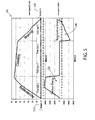
- FIG. 9 illustrates an initial timetable and an optimized timetable, wherein as first dwell time is shortened in the optimized timetable, others have to be lengthened to respect commercial speed.
- the distance (or time) between two trains is crucial in terms of security - when the headway is too short - and in terms of quality of service when it gets too long.
- the headway is obviously directly modified by the modification of dwell times; one has to know the limits of modification of these.
- Headways imply two kinds of tolerances: local and global.
- the local tolerance forces the headway to be within an interval centered on the initial headway (e.g., ⁇ 10%).
- the global tolerance acts as a "balance" between different headways. Indeed, to not degrade too much the quality of service, headways have to be not too different from each other to not create gaps between trains as shown in FIG. 10.
- FIG. 10 illustrates Train 1 and Train 2, wherein Train 2 is delayed to optimize energy consumption and pulls train 3 which is delayed as well. To understand it, one can imagine that every train is linked to others with a spring. If a train is delayed, then it pulls on other springs and other trains are delayed as well.
- This three dimension matrix represents the number of people going from a station to another in function of time as shown in Table A. It will be useful in some model refinements to formulate penalties on certain moves for optimization. For instance, a station which is considered as strongly used by passengers will not likely have its dwell time changed compared to another station where few people stop at.
- the origin/destination matrix can be delivered with an approximation of the amount of people using metro at each station. This refinement is of course to avoid degrading the quality of service.
- the matrix may be used in future development for testing the robustness of the optimization, by introducing perturbations within the matrix and verifying that the optimization remains intact.
- the following relates to algorithmic approaches to model energy flows in the railway network. Different formulations can be inferred regarding to the topology of the real system one wants to model and to the simplifications one has to make to be able to optimize the model in reasonable time. The following shows several ways to formulate different parts of the energy section of the data model.
- This formulation considers as the energy needed, thus the energy considered in optimization computation, the one which is effectively used to supply electrically the train.
- This model actually considers that the electric energy provided by electric stations is fully available without any loss anywhere on the network. This model is valid assuming that electric losses through materials and equipment can be considered as constant over a time period and then irrelevant for a relative optimization.
- This formulation prefers considering the energy drawn from electric provider needed to supply the train, possibly considering potential losses due to ohmic resistances in the third rail or in catenaries. This energy is logically higher than the energy eventually consumed by the train. This refinement is particularly important if it is considered the maximum traction energy issues.
- This simplification considers that a single electric station is providing electric energy on all points of the network.
- This simplification associated with the sink oriented energy counter, allows not considering the primary energy transportation which occurs between electric stations and trains accelerating. It permits focusing only on the secondary energy transportation, that is to say the exchange of energy from trains (braking) to electric stations or, depending on the model, directly from braking trains to accelerating trains.
- This model considers that trains are electrically supplied by different electric sub-stations, depending position on the network. For instance, one can consider that there is an electric sub-station at every metro station and that trains are drawing energy to the network from the electric sub-station/metro station they belong to at a particular time.
- This transportation includes the transfer of electric energy between the electricity provider and the train, counting different devices such as cables or transformers which can occur as intermediaries.
- This transportation includes the energy provided by regenerative brakes on trains to supply other trains, counting different devices such as cables or transformers which can occur as intermediaries.
- Direct exchange is a formulation that considers regenerative energy is directly shared between trains only via wires.
- Indirect exchange is a formulation that considers braking trains give back energy to the electricity provider which is able subsequently, to provide this energy to demanding trains. It is also possible to consider that regenerative energy is bought back by the electricity provider instead of being redistributed over the network
- This formulation allows the most accurate way to model ohmic losses. It is based on keeping track of trains over a grid which exactly represents the network topology. The losses are then simply computed, multiplying the distance between two electrically linked points by an attenuation rate. The main issue is that keeping track of trains geographically implies having an accurate model which includes distances and speeds. This formulation seems to be at first glance too much refined to have a simple and fast optimization program.
- interstation losses is a relaxation of the geographical topology. It only keeps track of the interstation (the area between two metro stations) where every metro is. So the losses are computed by checking the distance between two interstations and applying an attenuation rate as shown in Table B. For instance, if two metros are in the same station, the distance is 0, and so on. Table B - Attenuation rate in function of the distance between two interstations Interstation Distance 0 1 2 3 4 5+ Attenuation rate 1 0.9 0.7 0.4 0.1 0
- the attenuation decreases linearly along the distance between two points.
- the gradient would be chosen accordingly with experts.
- the attenuation is low on short distances but decreases strongly when distances do so.
- Catenaries, third rails, etc. have different ohmic resistances and each section/area is associated with equipment, so a particular attenuation function. If during an energy transfer, different equipment is used, then the losses are different along the different sections (e.g., heterogeneous equipment).
- a selection can be made between choosing to count or not devices which are intermediaries between two electric points, such as transformers, providers or trains. Every device can have an energetic efficiency that one has to take into account in the computation of the energy consumption (e.g., transfer equipment counting).
- the precision for the discretized data (e.g., discrete data) is chosen at 5s. It is then possible to optimize finely without altering quality of service. Moreover, most of state-of-art software works with a granularity of 5s.
- Table C illustrates data tables regarding an exemplary trip 1 and trip 2.
- T1 -> T2 T2 -> T1 Trip 1 3 5 Trip 2 4 6 Departure Time 0 240 500 Departure Time 50 295 550 Dead Run Time 120 120 120 135 135 135 Speed Profile Speed Profile T1 -> S1 norm norm norm norm T2 -> S4 normal normal Eco S1 -> S2 eco eco eco eco S4 -> S3 normal eco Eco S2 -> S3 eco normal eco S3 -> S2 normal normal Eco S3 -> S4 eco eco fast S2 -> S1 eco fast Fast S4 -> T2 fast fast fast S1 -> T1 fast normal Dwell Time Dwell Time S1 30 25 35 S4 30 25 30 S2 25 25 25 25 S3 30 25 25 S3 30 35 30 S2 30 40 25 S4 30 30 30 25 S1 30 30 30 25 T2 40 40 T1 40 40 40 40 Arrivals and departure times of trip 1 can be drawn from the data table above and the energy patterns of each interstation/speed profile.
- An interstation in accordance with a speed profile, will have a specific energy pattern (see Table D).
- This pattern represents the energy consumed (or generated) by a train within timeslots of 5 seconds. The duration of this pattern (in terms of timeslots) will be used to set the timetable of the trip.
- Table D Example of an energy pattern S1 -> S2 normal 5 sec Timeslot traction (kW.h) Comments - 0,00 dwell 1 1,39 traction 2 5,56 3 8,33 4 4,17 5 0,69 coasting 6 0,69 7 0,69 8 0,69 9 0,69 10 -4,17 braking 11 -2,08 12 -0,69 - 0,00 dwell
- This (dead run times) represents the time needed for a train to operate in terminal. This includes the change of direction and of driver. These figures are important to check that not too many trains are "jamming" in terminals during optimization.
- An attenuation matrix can be employed. Even if a metro line consist of several electric sub-stations and sections which supply energy to trains accordingly to their geographical position, consider that sections are interconnected so that regenerative energy from braking can be dispatched all along the line.
- the driving tension for metros is equal to 750V.
- the regenerative energy is equal to around 30-40% of the traction energy.
- the power peak of traction for a single train is equal to 3000kW and to 2000kW for the braking phase.
- a probabilistic value can be used to compute the attenuation which is done as follows: 1) If two trains are in the same interstation, their probable distance is 1/3 of the length of the interstation; and 2) If two trains are in two different interstations, their distance is equal to half of the length of the two interstations they belong to plus the length of the interstations which separate them.
- FIG. 11 illustrates an example of interstation lengths using the RER A path in Paris.
- Annex 3 explains how the figures are computed.
- a train is generating energy in interstation 2 (between National and Gare de Lyon) to supply a candidate in interstation 5 (between Auber and Charles de Gaulle - Etoile) then the energy supplied will be attenuated by 12.5%.
- Hypothesis 1 Regenerative energy of a braking train is given in priority to the closest candidate and so on until the braking train does not have any more energy remaining or any more trains are candidate.
- Hypothesis 2 if several trains generate energy, the one which generates the most supplies in priority.
- Headways are computed between adjacent trains on the line all along their respective trips. It is possible to easily compute headways at every station subtracting arrivals and departures of trains (see Table C) and checking headways are included in authorized intervals.
- the modifications of the timetable are the heart of the energy optimization. They consist in changing, under some constraints, the departure times of trains at every station and the speed profiles of trains at every interstation.
- the data table will compile all modifications of every trip at every station.
- the modifications will be directly used to change the energy timetable.
- the modifications are described by the delay in timeslots (so here in seconds) between the original driving pattern and the optimized one. If a departure is earlier than the original one, the delay will be negative and positive if it is later. Note that dead run times are a priori not modifiable.
- Table F Timetable modifications example
- T1 -> T2 Trip 1 3 5 Departure Time - 5 -10 Dead Run Time - - - Speed Profile
- the energy timetable is a function of the data table (which gives the departure times, the dwell times and the speed profiles), the energy patterns (which fill the energy consumption from the departure timeslot until the end of the pattern) and the timetable modifications (which modifies the pattern).
- the following innovation can reduce energy consumption in metros without adding specific hardware, by taking into account quality of service (QoS), and using existing time tables.
- QoS quality of service
- the system can reduce energy consumption by avoiding loss of regenerative energy. This may not be applicable when a train does not give back energy or when regenerative energy is saved (e.g., batters, super capacitors, reversible electrical substation, flywheels, in train, or trackside, etc.).
- the system can utilize a free optimization. There may be no specific hardware required (e.g., batteries, super capacitors, reversible electrical substation, flywheels, etc.). There can be a reduced cost for optimizing a timetable and there can be an objective of 5% savings.
- FIG. 5 illustrates energy consumption of a vehicle (e.g., a metro, a train, among others) on an interstation run in a graph 500.
- the graph includes a first terminal 510 and a second terminal 520 in which the vehicle can travel therebetween.
- the graph illustrates a traction energy 530 corresponding to the acceleration of the vehicle from the first terminal. Additionally, the graph illustrates a regenerative energy corresponding to the braking of the vehicle at the second terminal.
- FIG. 6 illustrates energy consumption of two vehicles (e.g., metros, trains, among others) in a graph 600.
- the graph illustrates two (2) unsynchronized vehicles (e.g., trains, metros, among others) in which the energy consumption is approximately 162000 kJ (e.g., 45 kWh).
- the first vehicle also referred to as train, metro, among others
- the second vehicle includes a traction energy 630 associated with accelerating and a regenerative energy 640 associated with braking.
- the energy consumption is at a high level due to each vehicle adding to the energy consumption.
- FIG. 7 illustrates energy consumption of a vehicle (e.g., a metro, a train, among others) in a graph 700.
- the graph illustrates two (2) synchronized vehicles in which the energy consumption is 133300 kJ (e.g., 37 kWh) (an amount lower than the amount in FIG. 6 for unsynchronized vehicles).
- the traction energy 630 of the second vehicle can overlap and correspond to the regenerative energy 620 of the first vehicle, wherein the second vehicle is accelerating and the first vehicle is braking. That there can be a suitable number of vehicles that allow overlap of an acceleration and braking and two vehicles is used as an example.
- QoS quality of service
- Energy optimization of timetable shall minimize the deviation of planned QoS (e.g., keeping the deviation under a threshold defined by the metro operator).
- the operator may accept more QoS deviations in off peak hours.
- there are more energy losses in off peak hours e.g., fewer train candidates).
- terminal departure times, dwell times, and speed profiles can be modified.
- Terminal departure times can be modified and may impact headways (e.g., not commercial speed).
- An optimized timetable can be loaded in most of "classical" automatic train stop (ATS) systems.
- Dwell times can be modified and can be changed by few seconds each time.
- the dwell times can be shortened or lengthened and may impact headways and/or commercial speed.
- Speed profiles can be modified.
- ATC and/or Automatic Train Operation generally allow different speed profiles.
- different speed profiles can include normal speed, accelerated speed, and economy (eco) mode.
- the modification of speed profiles may impact headways and/or commercial speed.
- Additional constrains can be headways, rolling stock availability, track availability, and QoS.
- Headways allowed by ATC/ATP can be hard constraints. ATP may never authorize a train to go under minimum headway.
- Rolling stock availability can also be hard constraints. There shall be available train for a train departure (typically a train cannot depart before arriving).
- Track availability can be a hard constraint.
- a terminal cannot contain more trains than platforms.
- QoS can be a soft (e.g., flexible) restraint.
- the subject innovation provides an accurate model for optimization and a model for the electric topology of the network.
- Minimizing modifications include two methods that have been tested 1) Tabu search (meta heuristics) and 2) genetic algorithms.
- Tabu search includes the following: start from one initial timetable, make a modification that minimizes objective, avoid making this modification for some iterations, and go back to making a modification that minimizes objective until termination criterion.
- Gs Genetic algorithms include the following: instantiate a population of timetables slightly different from the initial one, classify the timetables, mate them (e.g., crossover), mutate them, and go back to instantiating a population of timetables until termination criterion.
- the Tabu method can be tested on terminal departure time. There can be a modification of ⁇ -30,0,+30 ⁇ of any departure time in an off line timetable with a timeslot of 15s. The results show a 3% savings (using as example data of a Korean Metro line). The test can be limited based upon no model of energy attenuation and/or no verification of RSM/track availability.
- the GA method can be tested on dwell time modification.
- the dwell times can be changed by ⁇ -3s, 0s, 3s, 6s, 9s ⁇ in an off line timetable with time horizon of 1 hour (from 10am to 11am). With the use of GAs this provides a computation time of 45 minutes.
- the sample metro results provide the following: Initial consumption: 14360 kWh; After optimization: 13560 kWh; and Savings: 800 kWh / 5.6%.
- the test can be limited based upon the data is test data and nonexistent.
- an offline/online optimization there can be an offline/online optimization.
- the offline optimization can be with GA in which robustness is provided with many constraints and variables.
- Tabu method can be used for rapidity, adaptability, need to take into account others online classical regulation objectives (e.g., headway, regulation, passenger platform de-synchro, correspondence, safe haven, etc.).
- the online optimization can include criteria to trigger the optimization.
- the response time can be taken into account.
- T be the sample of a timetable and S the set of stations.
- I be the set of trains consisting of 1 train t 0 and n other trains. All trains stop at stations different from each other during the time horizon. Thus there are m • ( n + 1) stations in the metro line. The time can be discredited different moments that can be:
- a journey trip for a single train be a periodic succession of dwell times, accelerations, coasting times and braking.
- the interstation time is equal to 8 and the journey pattern is a periodic succession of:
- n trains have a journey length equal to 8 m - 1. So ⁇ k ⁇ ⁇ I ⁇ t o ⁇ there is a succession of m period of:
- the aim of the optimization is to synchronize accelerations of the n trains with the braking of t o .
- the timetable is synchronized if and only if trains which accelerate can be optimally synchronized with braking of t o .
- Theorem 1 The network can save m, energy units if and only if ⁇ is satisfiable.
- Example 1 Let ⁇ ⁇ ( x ⁇ y ⁇ ⁇ z ) ⁇ ( x ⁇ ⁇ y ⁇ z ) ⁇ ( ⁇ x ⁇ y ), the constructed timetable T is as follows, with t for travel at coasting speed, - quantity for braking , + quantity for
- the following relates to generatlized max flow problems in a lossy network.
- the notion of max flow has been introduced by Ford-Fulkerson in 1962 in [4] and has been a major research field in the 80's to find polynomial time algorithms.
- the max flow problem is the problem of maximizing a flow in a flow network.
- a flow network is a finite directed graph G ( V , E ) consisting of edges ( u , v ) ⁇ E with a capacity c(u, v ) and a flow f(u, v) ⁇ c(u, v) and at least two vertices ⁇ V , the source s which can produce flow and the sink t which can absorb flow.
- v ⁇ u ⁇ E f u ⁇ v which means that if a flow f (u, v) is entering at vertex ⁇ then ⁇ (u, v) f (u, v) is going out from v .
- the generalized max flow problem is to find a generalized flow f maximizing the excess function at sink e f ( t ).
- the generalized max flow model allows for formulating the computation of the objective function as a particular case of it.
- Edges consist in the virtual links between trains and energy. Then, there are three types of edges:
- a zero flow can correspond to an absence of regenerative energy transfer.
- a lossy network is a generalized network where a flow can decrease as it goes through edges.
- Theorem 2 A given flow is optimal if and only if the residual network does not contain any flow-generating cycle from which the sink t is reachable.
- a flow can be optimal even if this is not the maximum flow.
- a given flow is optimal if the way it is spread in the network minimizes losses along the edges.
- the highest-gain path is the path P from s to t such ⁇ ( i,j ) ⁇ P ⁇ ( i,j ) is maximized.
- Finding the optimal max flow in a generalized network is then equivalent to saturate the residual generalized network along highest-gain path.
- a generalized network consisting of 3 trains 1, 2 and 3 producing respectively 2, 3 and 4 units of energy and 3 trains A, B and C consuming respectively 2, 4 and 3 units of energy: with along edges the capacity and the gain for those different from 1.
- the heuristic consists in the idea of transferring the energy of each producer to respective closest consumers in the line. By doing that, the transfer of energy is optimal if producers are all independent from each other. Indeed, the choice of which producer will transfer its energy first is randomized so global optimum can be not reached.
- the following relates to computation time on real data.
- Our model has been tested with a one-hour time horizon, corresponding to 3600 timeslots, 30 metros and 496 dwell times to optimize.
- the objective function has a value 8544.4 a.u. at time to. After 450 iterations, total energy consumption is about 7884.5 a.u, that to say 7.7% saving.
- Table H shows the results. There is even with 6 second noise. The optimization is still saving 6.0% energy. This means that the optimized solution is saving energy, but also all its neighbour solutions.
- the objective in [7] is to minimize the energy peak, i.e. minimize the energy consumption of the timeslot of the time period where the energy consumption is maximum.
- regenerative energy is not considered in implementation even if the data model was taking it into account. There is then no need to use any attenuation matrix compiling Joule's effect as no energy transfer is possible.
- regenerative energy can be transferred in totality to an train consuming energy as long as the two trains are physically in the same electric sub station network.
- electric sub stations are not coupled and it is impossible to transfer energy from a point in the line belonging to an electric sub station to a point belonging to another one.
- FIG. 8 illustrates a flow chart of an exemplary embodiment of a method 500.
- a default timetable can be received in an offline mode, wherein the default timetable can be associated with a time schedule for two or more vehicles and at least one location.
- the default timetable can be adjusted by modifying at least one of a departure time of a vehicle, a dwell time of a vehicle, or a speed profile of a vehicle to estimate an overlap for a brake time for a first vehicle and an acceleration time for a second vehicle in the offline mode.
- the modified default timetable can be employed in real time for the two or more vehicles and the location.
- a portion of energy can be transferred from the first vehicle to the second vehicle based upon the modified default timetable in real time.
- the adjusted default timetable can be updated in real time to synchronize a brake time for a vehicle and an acceleration time for a vehicle by changing at least of a departure time of a vehicle, a dwell time of a vehicle, or a speed profile of a vehicle.
- the method can further include controlling the first vehicle or the second vehicle with a control signal based on the modified default timetable in real time.
- the method can further include tracking the vehicles in comparison with at least one of the modified timetable or a measured amount of energy, monitoring a threshold value related to the measured amount of energy, and updating the modified timetable based upon the threshold value or the tracking of the vehicles.
- the terms “may” and “may be” indicate a possibility of an occurrence within a set of circumstances; a possession of a specified property, characteristic or function; and/or qualify another verb by expressing one or more of an ability, capability, or possibility associated with the qualified verb. Accordingly, usage of “may” and “may be” indicates that a modified term is apparently appropriate, capable, or suitable for an indicated capacity, function, or usage, while taking into account that in some circumstances the modified term may sometimes not be appropriate, capable, or suitable. For example, in some circumstances an event or capacity can be expected, while in other circumstances the event or capacity cannot occur - this distinction is captured by the terms “may” and “may be.”
Landscapes
- Engineering & Computer Science (AREA)
- Business, Economics & Management (AREA)
- Economics (AREA)
- Physics & Mathematics (AREA)
- General Physics & Mathematics (AREA)
- Human Resources & Organizations (AREA)
- Strategic Management (AREA)
- Health & Medical Sciences (AREA)
- General Business, Economics & Management (AREA)
- Marketing (AREA)
- Mechanical Engineering (AREA)
- Tourism & Hospitality (AREA)
- Theoretical Computer Science (AREA)
- Water Supply & Treatment (AREA)
- Public Health (AREA)
- Entrepreneurship & Innovation (AREA)
- Quality & Reliability (AREA)
- Game Theory and Decision Science (AREA)
- Primary Health Care (AREA)
- General Health & Medical Sciences (AREA)
- Operations Research (AREA)
- Development Economics (AREA)
- Aviation & Aerospace Engineering (AREA)
- Automation & Control Theory (AREA)
- Remote Sensing (AREA)
- Radar, Positioning & Navigation (AREA)
- Train Traffic Observation, Control, And Security (AREA)
- Electric Propulsion And Braking For Vehicles (AREA)
- Traffic Control Systems (AREA)
Abstract
Description
- Embodiments of the subject matter disclosed herein relate to vehicle scheduling and control. Other embodiments relate to synchronizing two or more railway assets to optimize energy consumption.
- In light of various economic and environmental factors, the transportation industry has strived for solutions regarding sustainable energy as well as, or in the alternative, energy conservation. Conventional solutions include hardware such as, for instance, fly-wheels or super batteries, which alleviate the sustainable energy and/or energy conservation. Such hardware can be costly not only for the specific cost of the hardware but the cost routine maintenance thereof.
- It may be desirable to have a system and method for managing energy systems that differ from those that are currently available.
- In one embodiment, a system is provided. The system includes a first component configured to receive a timetable associated with two or more vehicles and at least one terminal. The system further includes a second component configured to modify at least one of a departure time of a vehicle or a dwell time of a vehicle to create a modified timetable that overlaps a brake time for a first vehicle and an acceleration time for a second vehicle.
- In one embodiment, a system is provided. The system includes a timetable associated with a first vehicle, a second vehicle, and a terminal, in which the timetable is a schedule of a time that the first vehicle and the second vehicle are at least one of arriving or departing the terminal. The system further includes a modify component configured to adjust the timetable to synchronize a brake duration of the first vehicle with an acceleration duration of the second vehicle for the terminal.
- In one embodiment, a method is provided. The method includes receiving a default timetable in an offline mode associated with a time schedule for two or more vehicles and at least one location. The method further includes adjusting the default timetable by modifying at least one of a departure time of a vehicle, a dwell time of a vehicle, or a speed profile of a vehicle to estimate an overlap for a brake time for a first vehicle and an acceleration time for a second vehicle in the offline mode. The method further includes employing the modified default timetable in real time for the two or more vehicles and the location. The method further includes transferring a portion of energy from the first vehicle to the second vehicle based upon the modified default timetable in real time. The method further includes updating the adjusted default timetable in real time to synchronize a brake time for a vehicle and an acceleration time for a vehicle by changing at least of a departure time of a vehicle, a dwell time of a vehicle, or a speed profile of a vehicle.
- Reference is made to the accompanying drawings in which particular embodiments and further benefits of the invention are illustrated as described in more detail in the description below, in which:
-
FIG. 1 is an illustration of an embodiment of a system for optimizing energy consumption by synchronizing a first vehicle and a second vehicle; -
FIG. 2 is an illustration of an embodiment of a system for generating an energy model utilized to synchronize a brake time for a vehicle and an acceleration time for a vehicle; -
FIG. 3 is an illustration of an embodiment of a system for controlling two or more vehicles based upon an optimized timetable that conserves energy by synchronizing a first vehicle and a second vehicle; -
FIG. 4 is an illustration of an embodiment of a system for creating an optimized timetable offline and employing such optimized timetable online to conserve energy by synchronizing a first vehicle and a second vehicle; -
FIG. 5 is an illustration of a graph related to energy consumption of a vehicle; -
FIG. 6 is an illustration of a graph related to energy consumption of two unsynchronized vehicles; -
FIG. 7 is an illustration of a graph related to energy consumption of two synchronized vehicles; -
FIG. 8 illustrates a flow chart of an embodiment of a method for modifying a timetable to synchronize a first vehicle and a second vehicle; -
FIG. 9 illustrates an initial timetable and an optimized timetable; -
FIG. 10 illustrates a first train timetable and a second train timetable; -
FIG. 11 illustrates an example of interstation lengths for a vehicle; and -
FIG. 12 illustrates an example of a flow determination. - Embodiments of the present invention relate to methods and systems for synchronizing two or more vehicle (e.g., railway, among others) assets to optimize energy consumption. A timetable associated with two or more vehicles and at least one terminal can be received. The timetable can be modified to create a modified timetable that overlaps a brake time for a first vehicle and an acceleration time for a second vehicle, wherein at least one of a departure time or a dwell time is modified. Furthermore, the second vehicle can transfer energy from the first vehicle based upon at least one of the modified timetable and the brake time overlapping with the acceleration time.
- With reference to the drawings, like reference numerals designate identical or corresponding parts throughout the several views. However, the inclusion of like elements in different views does not mean a given embodiment necessarily includes such elements or that all embodiments of the invention include such elements.
- The term "vehicle" as used herein can be defined as any asset that is a mobile machine that transports at least one of a person, people, or a cargo. For instance, a vehicle can be, but is not limited to being, a truck, a rail car, an intermodal container, a locomotive, a marine vessel, a mining equipment, a stationary power generation equipment, an industrial equipment, a construction equipment, and the like.
- It is to be appreciated that "associated with the two or more vehicles" refers to relating to one or more of the two or more vehicles.
-
FIG. 1 is an illustration of an exemplary embodiment of asystem 100 for optimizing energy consumption by synchronizing a first vehicle and a second vehicle. The system includes atimetable 110 associated with a first vehicle, a second vehicle, and a terminal, wherein the timetable is a schedule of a time that the first vehicle and the second vehicle are at least one of arriving or departing the terminal. The time table can be aggregated by adata collector 120. Moreover, thedata collector 120 can aggregate a static input and/or a dynamic input (discussed below). The system further includes amodify component 130 that optimizes thetimetable 110 based upon the aggregated information and adjusts (e.g., modifies) at least one of a dwell time for a vehicle located within a terminal, a departure time for a vehicle located within a terminal, and/or a speed profile for a vehicle for a terminal. Themodify component 130 generates an optimized timetable 140 (also referred to as the modified timetable), wherein theoptimized timetable 140 improves energy consumption. - For example, the optimized timetable synchronizes two or more vehicles located within a terminal such that while a vehicle is braking, another vehicle is accelerating. In particular, synchronizing a first braking vehicle with a second accelerating vehicle allows a portion of energy to transfer from the first braking vehicle to the second accelerating vehicle. The system provides synchronization for two or more vehicles without any additional hardware such as super capacitors, fly-wheels, among others. The system can be computer-implemented via software such that the modify component adjusts a timetable to create the optimized timetable.
- The optimized timetable or modified timetable can be implemented to two or more vehicles 150 (herein referred to as "
vehicles 150"). There can be a suitable number of vehicles such asvehicle 1 to vehicle D, where D is a positive integer. In particular, the vehicles can be automatically controlled, manually controlled (e.g., a human operator), or a combination thereof. In either event, the optimized timetable can be implemented, wherein at least one of a dwell time, a departure time, and/or a speed profile is adjusted to synchronize the vehicles. By way of example and not limitation, the vehicle can be a train, a railway vehicle, an electrical-powered vehicle, and the like. - As discussed, the system can include the data collector. The data collector can aggregate information related to a timetable, a static input, and/or a dynamic input (See DATA below). For instance, the data collector can aggregate suitable data related to the timetable, two or more vehicles, a terminal (e.g., a location, a station, etc.), and the like. By way of example and not limitation, the dynamic input can be a dwell time, a departure time, a speed profile, a portion of a timetable, among others. Moreover, for example, the static input can be, but is not limited to, a Quality of Service (QoS) constraint, a constraint, an energy model, a tolerance, an energy profile, a network topology, an electric efficiency, an origin/destination matrix, a portion of a timetable, an energy transportation, a loss of energy, among others. The static input and/or the dynamic inputs are described in more details below.
- By way of example and not limitation, the system can create a timetable to provide synchronization between two or more vehicles. For instance, a timetable can be created which takes into account at least one of a security constraint, a quality of service constraint, the issue of energy consumption, and the like. In another example, the system can optimize an existing timetable for two or more vehicles. In another example, the
system 100 can create a timetable for two or more vehicles as well as optimize an existing timetable for two or more disparate vehicles. For instance, two stations or terminals can include a set of vehicles respectively. The first set of vehicles for a first station can include an existing timetable that the system can modify or adjust to improve synchronization. Further, a timetable can be created for the second set of vehicles related to a second station. -
FIG. 2 is an illustration of an exemplary embodiment of asystem 200 for generating an energy model utilized to synchronize a brake time for a vehicle and an acceleration time for a vehicle. The system can include amodel generator 210 that creates energy model(s) that can be collected by the data collector and further utilized by the modify component (not shown). The model generator can create a suitable model or a model with a suitable aspect to implement the optimized timetable to synchronize two or more trains for energy conservation. The below models and generation of such models are solely for example and not to be seen as limiting on the subject innovation (see MODEL ENERGY below). - The model generator can receive a model that represents a condition or characteristic associated with an environment in which two or more vehicles will be synchronized for energy conservation. For instance, the model can be or related to, but is not limited to, energy accountings, network topologies, energy transportation, ohmic resistance loss, among others. These models can be utilized to create an energy model for an environment in which two or more trains are to be synchronized with an optimized timetable by adjusting at least one of a dwell time, a departure time, and/or a speed profile.
-
FIG. 3 is an illustration of an exemplary embodiment of asystem 300 for controlling two or more vehicles based upon an optimized timetable that conserves energy by synchronizing a first vehicle and a second vehicle. The system includes acontroller 310 that can implement a control to thevehicles 150 based at least in part upon the generated optimized timetable. For instance, the controller can identify a change in a currently used timetable compared to the optimized timetable and implement such change. For instance, the controller can implement a new dwell time, a new departure time, and/or a new speed profile. - The controller can be utilized for an automatically driven vehicle (e.g., no human operator) as well as, or in the alternative, a human operated vehicle, or a combination thereof. For instance, the controller can include an automatic component (not shown) that will directly implement controls based upon a change identified in the optimized timetable. Furthermore, the controller can include a manual component (not shown) that can utilize a notification component (not shown) and/or a buffer component (not shown). The manual component can facilitate controlling a vehicle that is operated by a human. The notification component can provide a signal, a message, or an instruction to the human operator. For instance, the notification component can provide an audible signal, a visual signal, a haptic signal, and/or a suitable combination thereof. The buffer component can further include a buffer of time that can take into account a delay that occurs from a human operator receiving a notification and implementing such notification. For example, the buffer component can mitigate human delay to implement the optimized timetable.
-
FIG. 4 is an illustration of an exemplary embodiment of asystem 400 for creating an optimized timetable offline and employing such optimized timetable online to conserve energy by synchronizing a first vehicle and a second vehicle. Thesystem 400 can include an offline mode (also referred to as "offline") and an online mode (also referred to as "online"). An offline mode can indicate a test environment or a modeled environment and an online mode can indicate a real time, real physical world environment. For instance, a real terminal station with vehicles can be an online environment whereas a computer simulation can be an offline environment. - The
system 400 allows a creation of an optimized timetable offline. Once the optimized timetable is created offline, the optimized timetable can be employed online. In particular, the controller can leverage the optimized timetable and implement specifics related thereto with vehicles. The online environment (also referred to as "online") can include amonitor 410, atrigger 420, and/or a modifycomponent 430. The monitor can track the vehicles in comparison with at least one of the optimized timetable and/or a measured amount of energy (e.g., energy conserved, energy consumed, energy transferred, among others). The trigger can include threshold values or triggers that will indicate whether or not the modify component will be utilized to update the optimized timetable based on the tracked information. - The following is a description related to energy optimization of metro timetables.
- Sustainable energy has been a major issue over the last years. Transportation is a major field concerned about energy consumption and the trend is to tend to optimize as much as possible the energy consumption in this industry, and in particular in mass rapid transit such as metros. Several hardware solutions, like fly-wheels or super batteries have been developed to reduce losses. However, these solutions involve buying and maintaining potentially costly material which can be difficult to economically justify.
- This application can describe a method which modifies dwell times to synchronize acceleration and braking of metros. Dwell times have the advantage to be updated in real time. To do that, a genetic algorithm is used to minimize an objective function - corresponding to the global energy consumption over a time horizon - computed with a linear program.
- The energy consumption in a metro line can be decreased by synchronizing braking and accelerations of metros. Indeed, an electric motor behaves as a generator when braking by transforming the kinetic energy into electrical energy. This energy, available in the third rail, has to be absorbed immediately by another metro in the neighborhood or is dissipated as heat and lost. The distance between metros which are generating energy and candidate metros induces that part of the transferred regenerative energy is lost in the third rail due to Joule's effect.
- Most timetables do not take into account energy issues. The tables usually have been created to maximize quality of service, security and other constraints like drivers' shift or weekend periods for instance. It is however possible to slightly modify current timetables to include some energy optimization. Here, energy consumption of a metro line can be minimized during a given time horizon by modifying the off-line timetable.
- As an example, the model can be restricted to a single metro line (no fork or loops) including 31 stations with two terminals A and B. All trips are done from A to B or B to A, stopping at all stations. The timetable, based on real data, is a bit more detailed than the one given to passengers; in addition to departure times at every station, it compiles also: 1) running times between every station; and 2) dwell times at every station.
- Dwell times represent the nominal waiting time of a metro in a given station. This time can be different regarding the stations but it is considered here that every metro have the same dwell time for a given station, not depending on the hour of the day.
- For every timeslot (1 second in our model), the position of metros (between which stations they are) is known and the energy they consume (positive energy or produce (negative energy). Contrary to timetables data which are real, energy data have been created following energy models. Units can be arbitrary: a value of 1 in this system corresponds to the energy consumed by a metro at full throttle during one second. Losses due to Joule's effect are compiled in an efficiency matrix. It details the percentage of energy which can be transferred from a point to another point in the line.
- The objective (1) is to minimize the energy consumption over a given time period, thus to minimize the sum of energy consumptions over every timeslot. If T is conserved the set of timeslots and yt the energy consumption of the line at timeslot t, then the objective function is:

- The better use of regenerative energy can prevent the client investing in costly solutions like changing this. The computation of yt can be seen as a formulation of a generalized max flow problem which can be formulated as an LP problem. The minimization of the objective function is done by modifying only dwell times to shift schedules slightly and to synchronize in better way accelerations and braking.
- As global energy consumption is optimized by modifying dwell times, the need to clarify what are the relevant dwell time for the formulation arises. The dwell times are computes as follows:
- Sets
- T: timeslots.
- I: metros.
- S: stations.
- Dr ⊂ I × S : relevant dwell times.
- Parameters
- Depi,s : arrival time t ∈ T of i ∈ I to the station, s ∈ S.
- Di,s : dwell time of i, s ∈ Dr .
- δ: minimal quantity for delaying/speeding up a dwell time.
- Variables
- di,s : optimized dwell time of metro i ∈ I at station s ∈ S.
- ni,s ∈ : number of times δ is applied to a dwell time i, s.

- Model

with
- Then these are the dwell times di,s ∈ Dr ⊂ I × S that the genetic algorithm will modify to minimize the objective function. Note that n can be unbounded. In the model, it is however bounded by small integers to stick on the quality of service issue and to keep having an invisible optimization for the final user.
- Modifying dwell times involves a new synchronization between metros. Every iteration of the genetic algorithm can be computed, resulting in an objective function. As explicated in (1), every timeslot represents an independent problem. The issue here is that it is hard to know exactly how regenerated energy will spread throughout third rail and other metros. Some models take as a hypothesis that metros can transfer entirely their regenerative energy to others only if they belong to the same electric sub-section. The hypothesis here is that energy is dissipating proportionally to the distance between two metros. Also, the hypothesis here is that the energy is spread in an optimal way, i.e., the model minimizes the loss of energy. Then, for a given timeslot there is:
- Sets
- I +: metros consuming energy.
- I -: metros producing energy.
- Parameters
-

-

- Ai,j : proportion of the energy produced by i ∈ I - transferable to j ∈ I + due to Joule's effect.
-
- Variables
- xi,j : proportion of the energy produced by i ∈ I - transferred to j ∈ I +.
- The LP model minimizes the energy consumed by spreading the energy produced in such a way

- By modifying only slightly the dwell times, it is considered that the algorithm never reaches non satisfiability (not satisfied) as it is stayed in tolerable intervals, e.g., for headways. Every individual in the population is represented by a two array table with metros in rows and stations in columns. Each cell represents a dwell time. Starting with initial dwell times, a population is created made of 100 individuals. Then every dwell time is randomized within a predefined domain, e.g., f-3s, 0s, +3s, +6s, +9sg. Finally, for every iteration, individuals are classified according to their objective function and selected. A crossover and mutation can be applied to them until convergence.
- The model has been tested with a one-hour time horizon, corresponding to 3600 timeslots, 29 metros, and 495 dwell times to optimize. The objective function has a value 8504 a.u. at time t0. After 450 iterations, total energy consumption is only 7939.4 a.u, that to say 6.6% saving. The computation lasts over 88 hours long on an
Intel Core 2 1.86GHz Linux PC. As this optimization is to minimize an off-line timetable, it can be allowed. - A real metro line is subject to minor disturbances that can affect the adherence to the timetable. To check the relevance of the optimization, there can be an added a random noise on optimized dwell times to quantify the robustness of the objective function. This noise consists in randomly modifying dwell times by ± δ s .
Table 1. Alteration of the objective function according to noise Noise (s) 1 3 6 Average on 100 tries (u.a.) 7964,9 7995,7 8028,4 Saving (%) 6,3 6,0 5,6 - Table 1 shows the results. It can be seen that even with 6 second noise (corresponding to 2 intervals of modification from time of parking/stationary), the objective function is still saving 5.6% energy. This means that the optimized solution is saving energy, but also all its neighbor solutions.
- This resolution method to optimize the energy consumption in a metro line seems promising and deserves more research. In particular, it is wanted to increase the number of parameters that can be modified, such as departure times in terminals or speed profiles. Effort can be made to also compare these results with other methods such as constraint programming. Eventually, decreasing computation time can allow this method to be used in a real-time context, in particular when it is about to optimize energy consumption after major incidents.
- The following is a description related to a data model for energy optimization.
- The following provides a comprehensive overview of the different data needed to formalize a model representing the energy consumption of trains and/or vehicles. It gives also a possible formulation of the model itself regarding the given data as well as different approaches for representing as best, and taking into account time computation, the energy consumption.
- Embodiments of the invention can be a software system used to decrease energy consumption in a metro line. This system allows a better synchronization of accelerating and braking metros, optimizing the use of regenerative energy produced by metros when braking.
- In an embodiment, the system uses as input the current timetable of a line. Including all possible regulation constraints like headways, the system modifies dwell times, departures times, and possibly speed profiles in a transparent way for the user. Indeed, the system takes into account quality of service by only slightly modifying the different parameters of the trip. To decrease energy consumption, the system has energy data of trains (their energy profile) as well as the topology of the line (how do electric sub stations work) to optimize train patterns. The output of the system, embedded in ATS, is a new version of the timetable, which may look like the old one but which is energy optimized.
- The system allows optimizing the use of regenerative energy due to braking metros (vehicles, trains, etc.). Indeed, if the regenerative energy is not consumed immediately by another metro in the line (if there is no other solutions like reversible electric sub stations or super capacitors), then this energy is lost as heat in the third rail. The regenerative energy, even if it does not decrease directly the overall energy consumption, permits to use less energy to start another metro which needs energy at the same time. Then the optimized reuse of regenerative energy indirectly decreases the total energy consumption.
- The better use of regenerative energy can prevent the client investing in costly solutions like changing his electric substations into reversible ones or embedding batteries in metros. The software approach as well as the minimal impact on quality of service can be seen by the client as a "free" optimization, because he can save energy just by clicking on a button "optimize", and not by adding new devices on the line.
- Conventional techniques provide different solutions to attempt to use the regenerative energy such as, but not limiting to, powering the air conditioning system in metros, charging embedded batteries, powering flywheels for later use, charging embedded super capacitors, supplying reversible electric substations, among others.
- Embodiments of the system further include a graphic user interface (GUI) that allows setting parameters of optimization in real time to make a system or metro line more efficient. The GUI can allow selection between optimized or actual timetables when perturbations occur.
- This model can be used in to minimize the energy consumption of trains over a period of time by software means. The optimization would indeed be done modifying the dwell times and departures at terminals and/or speed profiles. This optimization solution would be part of the solution of creating timetables and in another time, would be implemented for optimizing energy during real time regulation.
- The following is a description of the data utilized by an optimization model. To formulate a model accurate enough to forecast the gain in energy a fine optimization of timetables can perform, one needs the relevant data to do so. These data might be retrieved from a real case or made up internally, knowing the more realistic the data, the more relevant the optimization. The following is an example of data and is not to be limiting on the subject application.
- The data can be at least one of the following: feasible timetable (including departures/arrivals of stations/terminals, dwell times, train patterns/trips linking, stabling/unstabling pattern, etc.); energy profiles (depending on charge of train/vehicle, type of rolling stock, speed profile, etc.); electric network topology; electric efficiency of equipment; tolerances (for degrees of freedom, quality of service constraints, feasibility constraints, etc.); and origin/destination matrix.
- All data such as energy profiles, timetable scheduled hours and other including a time precision should be standardized. This precision will be chosen regarding different terms: precision of real systems; computing space available; and/or need for good precision for optimization. In an embodiment, the optimization and model can be discretized (e.g., discrete model) and not continuous.
- The optimization of the energy consumption in a metro line can be done on an already made timetable. The optimization can be a modification of several parameters of an initial timetable which minimizes the energy consumption and not a creation "from scratch" of a timetable considering energy issues. However, several possibilities are open to get this timetable.
- The timetable can be fully given, that is to say that it gives the departure times of every trip at every stop. This is typically the timetable given to passengers for information in railroad but not in mass transit, where the timetable is mostly given in terms of periodicity (e.g., every 2 minutes). In addition, the optimization needs the information about stabling/unstabling trains at terminals as well as rolling stock types, speed profiles associated to every trip.
- It can be given as well a map of departure times at terminals in addition with running times and dwell times at every station, those giving a full timetable when computed together. The information about stabling/unstabling and rolling stocks is still needed though.
- The energy model cannot be done without knowing exactly what are the energy consumption as well as the regenerative energy of the trains. The energy profile is however dependent to a lot of factors and several profiles - or at least a way to deduce several scenarios from a general profile - are needed.
- It is easier to move a train when empty than in peak hours when full of people. That is why one should have different charge-dependent energy profiles. It is also possible to have a charge-dependent rate which would be multiplied to an empty charge energy profile to get trains energy profiles dependent of their charge.
- Every type of train have different energy pattern, regarding their engine efficiency and their possible capability to provide regenerative energy, which can be taken into account.
- Most of timetabling software takes into account different speed profiles for a train. For instance, one can drive a train at normal, fast or economic speeds. These speed profiles can imply substantially similar amount of energy profiles.
- There is a difference between the input energy and the useful energy - i.e., the kinetic energy of the train - because real devices are never 100% efficient.
- Every wire, catenary, third rail or any other cable has an internal resistance greater than zero. With this data, the losses over cables are known, which would change the amount of regenerative energy a train is able to supply to another one. For instance, supplying a train at terminal B with the regenerative energy of a train braking in terminal A is not possible regarding the lineic resistance.
- In the same spirit, transformers and other electric devices (such as rolling stock) have a particular efficiency which has to be taken into account.
- Regarding the topology of the electric network of the metro line, it might not be possible to do several actions. It is important to know, over a particular example, if it is physically possible to, for instance, link directly to electrical points.
- The network can possibly be divided into electric sections which may be independent. By doing so, the trains are forced to supply other trains with regenerative energy only if they are in the same section, being unable to supply electricity in other sections if they are isolated.
- One has to consider the maximum amount of energy cables and equipment are able to withstand without deterioration. It is particularly important regarding the issues of maximum traction energy: a peak of energy occurring at a given time which can be above a certain limit.
- The tolerances are the levers which can be pulled to optimize the energy consumption. It has been chosen that the energy optimization would be done only by modifying the timetable, and not using hardware means such as fly wheels or embedded batteries. The tolerances given by the data will most likely be the acceptable intervals where the quality of service is not impacted.
- These parameters are the ones the optimization can directly modify to minimize the overall energy consumption.
- The stops in every station, normally given in the initial timetable, will be modified for optimizing the timetable. Regarding initial dwell times, one will be able to shorten or lengthen them in a certain amount given by tolerances. To not impact on quality of service, it will be also necessary to take care of a global shift all along a trip. For instance, every dwell time of a 20-station trip can be shortened by 5 seconds but the global shifting cannot be greater than 50 seconds (10 dwell times shortened).
- Similarly to dwell times, departure times can be shortened or lengthened depending on the need of the optimization. The main difference is that departure times might be shifted inside bigger intervals as the departure time affects much less the quality of service (nobody is waiting in the train at this moment).
- Speed profiles can be adjusted or modified to optimize the timetable (discussed above).
- These parameters are the ones the optimization will indirectly modify as they are dependent to ones the optimization can directly modify. These constraints can be unsatisfied during the process of optimization but the final optimized timetable must satisfy all the constraints, or the timetable will be considered unfeasible.
- The commercial speed represents the time a train is taking to go from its departure terminal to its arrival. Optimizing timetable should not affect too much this commercial speed. Whereas departure times do not affect it, dwell times do. Indeed, if a train is delayed by 10 seconds at one station but sticks to the timetable at the rest of its trip, then its commercial speed will be lengthened by 10 seconds.
- One has thus to take care of the commercial speed of trains, for instance by balancing the delays of trains; if a train is delayed at a station, it may leave earlier another station (see
FIG. 9). FIG. 9 illustrates an initial timetable and an optimized timetable, wherein as first dwell time is shortened in the optimized timetable, others have to be lengthened to respect commercial speed. - The distance (or time) between two trains is crucial in terms of security - when the headway is too short - and in terms of quality of service when it gets too long. The headway is obviously directly modified by the modification of dwell times; one has to know the limits of modification of these.
- Headways imply two kinds of tolerances: local and global. The local tolerance forces the headway to be within an interval centered on the initial headway (e.g., ± 10%). The global tolerance acts as a "balance" between different headways. Indeed, to not degrade too much the quality of service, headways have to be not too different from each other to not create gaps between trains as shown in
FIG. 10. FIG. 10 illustratesTrain 1 andTrain 2, whereinTrain 2 is delayed to optimize energy consumption and pullstrain 3 which is delayed as well. To understand it, one can imagine that every train is linked to others with a spring. If a train is delayed, then it pulls on other springs and other trains are delayed as well. - Different constraints are occurring in terminals which have to be taken into account for testing the feasibility of the timetable. Usually, only a limited amount of trains can take the actions of stabling, unstabling or returning in the same time at a particular terminal.
- This three dimension matrix represents the number of people going from a station to another in function of time as shown in Table A. It will be useful in some model refinements to formulate penalties on certain moves for optimization. For instance, a station which is considered as strongly used by passengers will not likely have its dwell time changed compared to another station where few people stop at. The origin/destination matrix can be delivered with an approximation of the amount of people using metro at each station. This refinement is of course to avoid degrading the quality of service.
- The matrix may be used in future development for testing the robustness of the optimization, by introducing perturbations within the matrix and verifying that the optimization remains intact.
Table A - Origin/Destination matrix for a 10 minutes section of 5 station stations Number Of people 1 2 3 4 5 1 2145 0 20 36 22 22 100 2 1287 10 0 23 30 37 100 3 564 31 19 0 33 17 100 4 3780 40 30 12 0 18 100 5 1546 17 37 28 18 0 100 - The following relates to algorithmic approaches to model energy flows in the railway network. Different formulations can be inferred regarding to the topology of the real system one wants to model and to the simplifications one has to make to be able to optimize the model in reasonable time. The following shows several ways to formulate different parts of the energy section of the data model.
- The way one is counting the energy consumed over a period of time obviously modifies the accuracy of the model. However it might be possible to show that the differences on counting energy influence only the absolute final value and not the relative gain of energy allowed by an optimization. Some simplifications on how to count energy may thus be conceivable if the output of our model is a relative gain of energy compared to the initial solution. The need of refining the model is however essential if the output of the model considers absolute values like the maximum traction energy.
- This formulation considers as the energy needed, thus the energy considered in optimization computation, the one which is effectively used to supply electrically the train. This model actually considers that the electric energy provided by electric stations is fully available without any loss anywhere on the network. This model is valid assuming that electric losses through materials and equipment can be considered as constant over a time period and then irrelevant for a relative optimization.
- This formulation prefers considering the energy drawn from electric provider needed to supply the train, possibly considering potential losses due to ohmic resistances in the third rail or in catenaries. This energy is logically higher than the energy eventually consumed by the train. This refinement is particularly important if it is considered the maximum traction energy issues.
- This formulation considers that all points of a network (most commonly a single metro line) are electrically linked. This means that a braking train would be able to provide energy to any given train accelerating at any point of the line.
- This formulation considers that the network is divided into independent sections which are electrically isolated from each other. This means that a braking train would be able to provide its energy to trains accelerating only if they are in the same area or section.
- This simplification considers that a single electric station is providing electric energy on all points of the network. This simplification, associated with the sink oriented energy counter, allows not considering the primary energy transportation which occurs between electric stations and trains accelerating. It permits focusing only on the secondary energy transportation, that is to say the exchange of energy from trains (braking) to electric stations or, depending on the model, directly from braking trains to accelerating trains.
- This model considers that trains are electrically supplied by different electric sub-stations, depending position on the network. For instance, one can consider that there is an electric sub-station at every metro station and that trains are drawing energy to the network from the electric sub-station/metro station they belong to at a particular time.
- This transportation includes the transfer of electric energy between the electricity provider and the train, counting different devices such as cables or transformers which can occur as intermediaries.
- This transportation includes the energy provided by regenerative brakes on trains to supply other trains, counting different devices such as cables or transformers which can occur as intermediaries.
- Direct exchange is a formulation that considers regenerative energy is directly shared between trains only via wires.
- Indirect exchange is a formulation that considers braking trains give back energy to the electricity provider which is able subsequently, to provide this energy to demanding trains. It is also possible to consider that regenerative energy is bought back by the electricity provider instead of being redistributed over the network
- One can consider the electric transportation through wires, catenaries and third rails as perfect, that is to say that electric energy provided by a device on the network would be usable fully and instantaneously by any other device of the network. It is obvious that for having a more accurate model, one has to consider ohmic resistance losses occurring in all cables. These energy losses can be considered on the primary energy transportation, the second energy transportation or both.
- This formulation (geographic losses) allows the most accurate way to model ohmic losses. It is based on keeping track of trains over a grid which exactly represents the network topology. The losses are then simply computed, multiplying the distance between two electrically linked points by an attenuation rate. The main issue is that keeping track of trains geographically implies having an accurate model which includes distances and speeds. This formulation seems to be at first glance too much refined to have a simple and fast optimization program.
- This formulation (interstation losses) is a relaxation of the geographical topology. It only keeps track of the interstation (the area between two metro stations) where every metro is. So the losses are computed by checking the distance between two interstations and applying an attenuation rate as shown in Table B. For instance, if two metros are in the same station, the distance is 0, and so on.
Table B - Attenuation rate in function of the distance between two interstations Interstation Distance 0 1 2 3 4 5+ Attenuation rate 1 0.9 0.7 0.4 0.1 0 - Depending on the network and physical constraints given by experts, it is possible to set different functions of attenuation.
- The attenuation decreases linearly along the distance between two points. The gradient would be chosen accordingly with experts.
- The attenuation is low on short distances but decreases strongly when distances do so.
- It is considered here that the different energy transportation devices (cables, catenaries, third rails...) have the same ohmic resistance and thus the energy loss along distance is simply a function of an attenuation rate (e.g., homogeneous equipment).
- Catenaries, third rails, etc. have different ohmic resistances and each section/area is associated with equipment, so a particular attenuation function. If during an energy transfer, different equipment is used, then the losses are different along the different sections (e.g., heterogeneous equipment).
- A selection can be made between choosing to count or not devices which are intermediaries between two electric points, such as transformers, providers or trains. Every device can have an energetic efficiency that one has to take into account in the computation of the energy consumption (e.g., transfer equipment counting).
- Beyond the several possibilities given by all different sorts of data one could get, one model with a particular shape for data has been chosen for a first implementation. It follows the formulation of past work adding some refinements in terms of computing energy. The shape of the important data needed as soon as possible is explicated below.
- The precision for the discretized data (e.g., discrete data) is chosen at 5s. It is then possible to optimize finely without altering quality of service. Moreover, most of state-of-art software works with a granularity of 5s.
- The below Table C illustrates data tables regarding an
exemplary trip 1 andtrip 2.T1 -> T2 T2 -> T1 Trip 1 3 5 Trip 2 4 6 Departure Time 0 240 500 Departure Time 50 295 550 Dead Run Time 120 120 120 135 135 135 Speed Profile Speed Profile T1 -> S1 norm norm norm T2 -> S4 normal normal Eco S1 -> S2 eco eco eco S4 -> S3 normal eco Eco S2 -> S3 eco normal eco S3 -> S2 normal normal Eco S3 -> S4 eco eco fast S2 -> S1 eco fast Fast S4 -> T2 fast fast fast S1 -> T1 fast fast normal Dwell Time Dwell Time S1 30 25 35 S4 30 25 30 S2 25 25 25 S3 30 25 25 S3 30 35 30 S2 30 40 25 S4 30 30 25 S1 30 30 25 T2 40 40 40 T1 40 40 40 trip 1 can be drawn from the data table above and the energy patterns of each interstation/speed profile.
Trip 1Table C -Shape for data formatting Journey T1D S1A S1D S2A S2D S3A S3D S4A S4D T2A T2D Time 0 120 150 300 325 475 505 655 685 785 825 A=Arrival
D=Departure - An interstation, in accordance with a speed profile, will have a specific energy pattern (see Table D). This pattern represents the energy consumed (or generated) by a train within timeslots of 5 seconds. The duration of this pattern (in terms of timeslots) will be used to set the timetable of the trip.
Table D - Example of an energy pattern S1 -> S2 normal 5 sec Timeslot traction (kW.h) Comments - 0,00 dwell 1 1,39 traction 2 5,56 3 8,33 4 4,17 5 0,69 coasting 6 0,69 7 0,69 8 0,69 9 0,69 10 -4,17 braking 11 -2,08 12 -0,69 - 0,00 dwell - This (dead run times) represents the time needed for a train to operate in terminal. This includes the change of direction and of driver. These figures are important to check that not too many trains are "jamming" in terminals during optimization.
- An attenuation matrix can be employed. Even if a metro line consist of several electric sub-stations and sections which supply energy to trains accordingly to their geographical position, consider that sections are interconnected so that regenerative energy from braking can be dispatched all along the line.
- This hypothesis implies taking into account Joule effect in third rail. The lineic resistance of the third rail is equal to 7µΩ/m.
- The driving tension for metros is equal to 750V.
- The regenerative energy is equal to around 30-40% of the traction energy. The power peak of traction for a single train is equal to 3000kW and to 2000kW for the braking phase.
- Consider after some computation (see below Annex 1) that the attenuation is equal to 1.65%/km. It means that if a braking train is able to produce 3MJ, it will be however able to supply a train at 5km far from it with only 2.75MJ.
- Every given time, it will be possible to know at which interstation (the line between two stations) a train is, knowing the journey pattern and the time pattern of every train. Then, when a train will brake to supply candidate trains on the line, it will be necessary to compute the attenuation of the energy along the third rail.
- To compute the attenuation between two interstations, multiply the attenuation rate by the probable distance between two trains.
- For instance, if two trains are in the same interstation, one cannot know exactly where they are and what the distance which separates them is.
- That is why a probabilistic value can be used to compute the attenuation which is done as follows: 1) If two trains are in the same interstation, their probable distance is 1/3 of the length of the interstation; and 2) If two trains are in two different interstations, their distance is equal to half of the length of the two interstations they belong to plus the length of the interstations which separate them.
- The example below (
FIG. 11 and Table E) shows how an attenuation matrix will look like.FIG. 11 illustrates an example of interstation lengths using the RER A path in Paris.Annex 3 explains how the figures are computed. In the example, if a train is generating energy in interstation 2 (between Nation and Gare de Lyon) to supply a candidate in interstation 5 (between Auber and Charles de Gaulle - Etoile) then the energy supplied will be attenuated by 12.5%.Table E - Attenuation matrix related to FIG. 11 1 2 3 4 5 6 1 1,65 3,8 7,76 12,1 16,3 22,7 2 3,8 0,99 3,96 3,22 12,5 18,9 3 7,76 3,96 1,65 4,37 14,9 14,9 4 12,1 3,22 4,37 1,16 4,13 10,6 5 16,3 12,5 8,5 4,13 1,49 6,44 6 22,7 18,9 14,9 10,6 6,44 2,81 - In most cases, power peaks are computed independently for each substation. However, total energy consumption is computed globally. One problem when computing sum of energy consumptions is to compute the attenuation of regenerative energy. Indeed, if you consider in a timeslot one regenerative train and two candidates trains for its energy, you cannot solely subtract the regenerative of the sum, you have to compute the attenuation for giving energy to every candidate and not counting it in the sum of energy consumptions.
- Hypothesis 1: Regenerative energy of a braking train is given in priority to the closest candidate and so on until the braking train does not have any more energy remaining or any more trains are candidate.
- Hypothesis 2: if several trains generate energy, the one which generates the most supplies in priority.
- Hypothesis 3: if no more trains are candidate while some regenerative energy remains, this energy is considered lost and the sum of energy consumptions is equal to 0.
- See the algorithm in section below referenced
Annex 2 for more details. - Headways are computed between adjacent trains on the line all along their respective trips. It is possible to easily compute headways at every station subtracting arrivals and departures of trains (see Table C) and checking headways are included in authorized intervals.
- These authorized intervals are expressed in terms of percentage. For instance, possible headways for an optimization would be in this interval: 0.9 x Initial Headway < Authorized Headway < 1.1 x Initial Headway.
- Commercial speed is the time a train takes to cover its whole trip. As well as headways, commercial speed must stay in an authorized interval after optimization. However, it may be considered different tolerances regarding the daytime: tolerances will be looser during off-peak hours for instance.
- The modifications of the timetable are the heart of the energy optimization. They consist in changing, under some constraints, the departure times of trains at every station and the speed profiles of trains at every interstation. The data table will compile all modifications of every trip at every station. The modifications will be directly used to change the energy timetable. The modifications are described by the delay in timeslots (so here in seconds) between the original driving pattern and the optimized one. If a departure is earlier than the original one, the delay will be negative and positive if it is later. Note that dead run times are a priori not modifiable.
- Here is an example (Table F) of timetable modifications:
Table F - Timetable modifications example T1 -> T2 Trip 1 3 5 Departure Time - 5 -10 Dead Run Time - - - Speed Profile T1 -> S1 - fast - S1 -> S2 - normal - S2 -> S3 - - - S3 -> S4 normal - normal S4 -> T2 - - - Dwell Time S1 5 - 10 S2 -5 - 5 S3 10 -5 5 S4 - -10 - T2 - - - - In
trip 1, the speed profile for interstation S3 -> S4 changes from economic to normal when the dwell time at station S3 fortrip 3 will be shortened by 5 seconds. - Basically, the energy timetable is a function of the data table (which gives the departure times, the dwell times and the speed profiles), the energy patterns (which fill the energy consumption from the departure timeslot until the end of the pattern) and the timetable modifications (which modifies the pattern).
- It compiles also the section where is every train at every timeslot to compute the energy consumption.
- Considering a single train can be supplied for traction up to 3MW and power peak in regenerative braking is equal to 2/3 of this amount, so 2MW. Considering nominal voltage of the line is 750V. Considering lineic resistance of third rail is 7µΩ/m. Considering braking lasts 15 seconds and generates electricity from 2MW to 0 following a linear curve.


Knowing that
Where Wheat is the energy dissipated due to Joule's law and Pheat the power dissipated,
That
Where Wheat is the energy dissipated due to Joule's law and Pheat the power dissipated,
That
Where Rlineic is equal to the lineic resistance of the third rail, D the distance between the regenerative train and the candidate and I the intensity
With
Thanks to Ohm law, U being the voltage,
We have
So

With D = 1km.
So the attenuation for 1 km of distance is equal to -

For a given timeslot: - SETS:
- Trains (relevant at this given timeslot)
- Givers = {i, ∀i ∈ Trains / Ei < 0} ordered by E descend
Candidates = {i, ∀i ∈ Trains /Ei > 0}
- PARAMETERS:
- Pi = geographical position of i ∈ Trains
- Eni = energy consumed (or generated)by i ∈ Trains
- Mi,j = rate of attenuation between i ∈ Trains and j ∈ Trains
- VARIABLES:
- X = energy consumption in the timeslot
- Ei = energy consumed effectively by i ∈ Trains
- Di = ohmic resistance distance of i E Candidates to a given train
subject to


       for all (i in Trains)
              E(i) = En(i);
       for all (i in Givers)
              if(Candidates = {})
                     break;
              for all (j in Candidates)
                     D(j)=M(P(i),P(j));
              Set CandidatesRelative = Candidates ordered by D ascend;
              while(CandidatesRelative != {} ∥ E(i) != 0)
                     if(E(j) > E(i)*D(j))
                            E(j) = E(j) - E(i)*D(j);
                            E(i) = 0;
                     else
                            E(i) = E(i) - E(j)*D(j);
                            E(j) = 0;
                            remove j from CandidatesRelative;
                            remove j from Candidates;
       X = sum(i in Trains)(E(i));
       if(X < 0)
              X=0;
       return X;
- The objective function. The physical quantity can take several forms.
When [1] and [7] are minimizing power peaks ( PP ) i.e. max t∈ T yt this model minimizes the global energy consumption of the line (G), i.e. Σ t∈T yt
- The variables. Different quantities can be modified to optimize any given objective function. One can consider three different variables that can be modified in a timetable:
- The departure times (D), or the timeslot when a particular trip is starting from its first station. This is what can be modified in [7] or [8].
- The dwell times ( d ), or the time lasted for a train in every station.
- The speed profiles ( s ). It is common to have several profiles for a train to cross two stations; typically a nominal one, a full speed and an economic one. Changing speed profiles allows to modify the timetable as well as the energy curve.
- The energy spreading. One can add some subtleties to the model to stick more to real situations. In particular, the way the energy is spread throughout the third rail is primary:
- The simplest model allows regenerative energy to be totally spread in all the metro line (wJ for "without Joule's effect"), like in [7].
- In the other way, the attenuation of regenerative energy when it passes in third rail can be formalized ( J ) like in our model, by for instance having an attenuation matrix compiling losses between different points of interest of the line. Note that the model wJ can be done by having a trivial attenuation matrix.
- Also, electric sub stations can be ( nC ), or not, coupled ( C ). It means that sometimes, it may not be possible to send regenerative energy from a point of the line to another due to the independence of two sub networks in the electric system. This independence can also be done via an attenuation matrix by attenuating completely points which are not belonging to the same electric sub station.

where every li,j is a literal of the form Xk or ¬Xk for 1 ≤ k ≤ n.
For every 1 ≤ k ≤ n and 1 ≤ i ≤ m, one can pose

- a dwell time, dk i
- an acceleration ak,i
- a braking bk,i
- a coasting time ck,i .
- a braking phase b0,i = 1
- a dwell time d0,i = 5
- an acceleration phase a0,i = 1
- a coasting phase c0,i = 1.
- b k,i
k = 1 and b k,0 = 0 - dk,i
k = 3 + uk,ik and d k,1 = 3 + uk,ik + δ k with δk ∈ {-1,1} - ak,i
k = 1 - ck,i
k = 3-uk,ik .
-
Lemma 1. For every timetable T' derived from T with δ' there exist k ≥ I and a time t such that T'k,t = - T' 0, t = + and a station i such that t = 8 • i - 4, and there exists a j such that li,j = Xk' or li,j = ¬Xk' and δ'k',1 = - 1 if li,j = ¬Xk' and
- Proof. For every 1 ≤ i ≤ m, let t = 8 • i - 5. Then T0,t = -. For every k' ≥ 1, if there exists a j such that li,j = Xk', then uk'i = -1 and Tk',t-1 = +, therefore if δ'k',1 = 1 then T'k',t = +. Similarly, if here exists a j such that li,j = ¬Xk', then uk',i = 1 and T'k',t+1 = +, therefore if δ'k',1 = -1 then T'k',t = +.
- Conversely, if there exist k, k' and a time t such that T'k,t = - and T'k',t = +. Note that there is T0,t = + only if t = 8 • i + 2, there is, for k ≥ 1, Tk,t = + only if t = 8 • i - 5 + uk,i, with -1 < uk,i < 2, and there is, for k ≥ 1, Tk,,t = — only if t = 8 • i- 1. Therefore, k = 0 and k' ≥ 1 and there exists an i such that t = 8 • i - 5. Since T'k',t = +, there is either δ' k',1 = - 1 or δ' k',1 = 1. If δ' k,1 = - 1, then uk',i = 1 and there exists j such that li,j = ¬Xk'. Similarly, if δ' k',1 = 1, then uk',i = - 1 and there exists j such that li,j = Xk'.
- Proof. If φ is satisfiable, there exists a valuation ν such that ν(φ) ⇔ 1. Consider the timetable T' derived from T with for every 1 ≤ k ≤ n, δ'k',1 = 1 if ν(Xk ) = 1 and δ' k',1 = -1 if ν(Xk ) = 0. For every
clause 1 ≤ i ≤ m, since ν(φ) ⇔ 1, there exists a j such that ν(li,j ) = 1: that is to say, either δ' k',1 = -1 if li,j = ¬Xk or δ'k',1 = 1 if li,j = Xk. Therefore, according tolemma 1, for t = 8 • i - 5, there is T'0,t = - and T'k,t = +. So it is possible to save one energy unit at time t = 8 • i - 5 for every 1 ≤ i ≤ m. - Conversely, if there is a timetable T' derived from T with δ' which saves m energy unit, therefore according to
lemma 1, these saves occur at times t = 8 • i - 5 for 1 ≤ i ≤ m. Consider the valuation ν such that for every 1 ≤ k ≤ n, ν(Xk ) = 1 if δ' k,1 = 1, ν(Xk ) = 0 otherwise. For everyclause 1 ≤ i ≤ m, there is a save at time t = 8 • i — 5. Therefore, according tolemma 1, there exist k and j such that either l i,j = Xk or li,j = ¬Xk and either δ' k',1 = - 1 if li,j = ¬ Xk or δ' k',1 = 1 if li,j = Xk. That is to say ν(li,j ) = 1.
- t o t t t - d d d d d + t - d d d d d + t - d d d d d + t
- x d d + t t t t - d d + t t t t - d d d d + t t
- y d d + t t t t - d d d d + t t - d d + t t t t
- z d d d d + t t - d d + t t t t - d d d d d + t
which means that if a flow f (u, v) is entering at vertex ν then γ(u, v) f (u, v) is going out from v.
- a source s
- vertices corresponding to trains that produce energy (I -)
- vertices corresponding to trains that consume energy (I +)
- a sink t.
- The edges starting from the source which represents the virtual energy which is given to trains that produce energy. The source virtually gives in the graph energy to trains ∈ Γ with an efficiency of 1.


- The edges virtually linking trains that produce energy to those which consume it. Indeed, producers are potentially able to distribute their energy to any consumer, even several consumers. The difference in the distribution is the efficiency along the edge representing the Joule's effect losses directly proportional to the distance between trains.


- The edges going from consumers to the sink represent the energy that has effectively been saved during the transfer of regenerative energy. The capacity of these edges ensures that a consumer cannot get more energy than it can absorb.


with the capacities of edges representing the energy consumption of accelerating trains and the flow the regenerative energy they absorbed.

- 1: while list_of_producers ≠ 0 do
- 2: Choose one producer.
- 3: while producer energy > 0 do
- 4: if list_of_consumers = 0 then
- 5: finish
- 6: Choose closest consumer.
- 7: if producer has more energy to transfer than consumer needs then
- 8: Transfer this amount and remove consumer off the list.
- 9: else
- 10: Transfer totality of remaining producer energy to the consumer.
- 11: Remove producer off the list.
- 12: finish
| Noise (s) | 1 | 3 | 6 |
| Average on 100 tries (u.a.) | 7917.6 | 7984.4 | 8029.7 |
| Saving (%) | 7.3 | 6.6 | 6.0 |

- 1. A system, comprising:
- a first component configured to receive a timetable associated with two or more vehicles and at least one terminal; and
- a second component configured to modify a parameter associated with at least one of a first vehicle or a second vehicle of the two or more vehicles to create a modified timetable that overlaps a brake time for the first vehicle and an acceleration time for the second vehicle.
- 2. The system of
clause 1, wherein the parameter is at least one of a departure time of the first vehicle or the second vehicle, a dwell time of the first vehicle or the second vehicle, or a speed profile of the first vehicle or the second vehicle. - 3. The system of
clause 1 orclause 2, wherein the second vehicle is configured to transfer a portion of energy from the first vehicle based upon at least one of the modified timetable and the brake time overlapping with the acceleration time. - 4. The system of any preceding clause, wherein the second component is configured to modify the parameter associated with at least one of the first vehicle or the second vehicle to create the modified timetable that overlaps a brake time for the second vehicle and an acceleration time for the first vehicle.
- 5. The system of any preceding clause, where the first vehicle is configured to transfer a portion of energy from the second vehicle based upon at least one of the modified timetable and the brake time for the second vehicle overlapping with the acceleration time for the first vehicle.
- 6. The system of any preceding clause, further comprising:
- a third component configured to aggregate a static input related to at least one of the two or more vehicles, the terminal, an energy model, or a quality of service constraint; and
- the second component further configured to create the modified timetable that overlaps the brake time for the first vehicle and the acceleration time of the second vehicle based on the static input.
- 7. The system of any preceding clause, further comprising:
- a fourth component configured to aggregate a dynamic input related to at least one of the two or more vehicles, the terminal, an in-use dwell time for the first vehicle or the second vehicle, an in-use departure time for the first vehicle or the second vehicle, or an in-use speed profile for the first vehicle or the second vehicle; and
- the second component further configured to create the modified timetable that overlaps the brake time for the first vehicle and the acceleration time of the second vehicle based on the static input.
- 8. The system of any preceding clause, further comprising:
- a fifth component configured to create at least one energy model to represent a portion of energy used by at least one of the terminal, the first vehicle, or the second vehicle; and
- the second component further configured to create the modified timetable that overlaps the brake time for the first vehicle and the acceleration time of the second vehicle based on the at least one energy model.
- 9. The system of any preceding clause, wherein the at least one energy model relates to at least one of a network topology for the terminal, an energy transportation between at least two of the first vehicle, the second vehicle, and a track for the first vehicle or the second vehicle, an ohmic resistance loss, or an equipment loss.
- 10. The system of any preceding clause, further comprising a controller that is configured to generate and communicate a control signal to the first vehicle or the second vehicle based on the modified timetable, wherein the control signal is used with an automated control of the first vehicle or the second vehicle or a manual control of the first vehicle or the second vehicle.
- 11. The system of any preceding clause, further comprising a sixth component that is configured to implement a buffer time to compensate for a human reaction time delay related to implementing the control signal for the first vehicle or the second vehicle.
- 12. The system of any preceding clause, wherein the second component is configured to create the modified timetable in an offline environment that corresponds to data representative of the terminal.
- 13. The system of any preceding clause, wherein the second component is configured to employ the modified timetable created in the offline environment within an online environment of the terminal.
- 14. A method, comprising:
- receiving a default timetable in an offline mode associated with a time schedule for two or more vehicles and at least one location;
- adjusting the default timetable by modifying at least one of a departure time associated with the two or more vehicles, a dwell time associated with the two or more vehicles, or a speed profile associated with the two or more vehicles to estimate an overlap for a brake time for a first vehicle of the two or more vehicles and an acceleration time for a second vehicle of the two or more vehicles in the offline mode;
- employing the adjusted default timetable in real time for the two or more vehicles and the location;
- transferring a portion of energy from the first vehicle to the second vehicle based upon the adjusted default timetable in real time; and
- updating the adjusted default timetable in real time to synchronize a brake time associated with the two or more vehicles and an acceleration time associated with the two or more vehicles by changing at least of a departure time associated with the two or more vehicles, a dwell time associated with the two or more vehicles, or a speed profile associated with the two or more vehicles.
- 15. The method of any preceding clause, further comprising controlling the first vehicle or the second vehicle with a control signal based on the adjusted default timetable in real time.
- 16. The method of any preceding clause, further comprising:
- tracking the two or more vehicles in comparison with at least one of the adjusted timetable or a measured amount of energy;
- monitoring a threshold value related to the measured amount of energy; and
- updating the adjusted timetable based upon the threshold value or the tracking of the vehicles.
- 17. A system, comprising,
a timetable associated with a first vehicle, a second vehicle, and a terminal, wherein the timetable comprises a schedule of a time that the first vehicle and the second vehicle are at least one of arriving or departing the terminal; and
a modify component configured to adjust the timetable to synchronize a brake duration of the first vehicle with an acceleration duration of the second vehicle for the terminal. - 18. The system of any preceding clause, wherein the timetable includes at least one of a first vehicle dwell time for the terminal, a first vehicle departure time for the terminal, or a first vehicle speed profile related to the terminal and the first vehicle.
- 19. The system of any preceding clause, wherein the timetable includes at least one of a second vehicle dwell time for the terminal, a second vehicle departure time for the terminal, or a second vehicle speed profile related to the terminal and the second vehicle.
- 20. The system of any preceding clause, wherein the second vehicle is configured to transfer a portion of energy from the first vehicle based upon the synchronization.
Claims (15)
- A system (100), comprising:a first component (120) configured to receive a timetable associated with two or more vehicles (150) and at least one terminal; anda second component (130) configured to modify a parameter associated with at least one of a first vehicle or a second vehicle of the two or more vehicles (150) to create a modified timetable that overlaps a brake time for the first vehicle and an acceleration time for the second vehicle.
- The system of claim 1, wherein the parameter is at least one of a departure time of the first vehicle or the second vehicle, a dwell time of the first vehicle or the second vehicle, or a speed profile of the first vehicle or the second vehicle.
- The system of claim 1 or claim 2, wherein the second vehicle is configured to transfer a portion of energy from the first vehicle based upon at least one of the modified timetable and the brake time overlapping with the acceleration time.
- The system of any preceding claim, wherein the second component is configured to modify the parameter associated with at least one of the first vehicle or the second vehicle to create the modified timetable that overlaps a brake time for the second vehicle and an acceleration time for the first vehicle.
- The system of any preceding claim, where the first vehicle is configured to transfer a portion of energy from the second vehicle based upon at least one of the modified timetable and the brake time for the second vehicle overlapping with the acceleration time for the first vehicle.
- The system of any preceding claim, further comprising:a third component configured to aggregate a static input related to at least one of the two or more vehicles, the terminal, an energy model, or a quality of service constraint; andthe second component further configured to create the modified timetable that overlaps the brake time for the first vehicle and the acceleration time of the second vehicle based on the static input.
- The system of any preceding claim, further comprising:a fourth component configured to aggregate a dynamic input related to at least one of the two or more vehicles, the terminal, an in-use dwell time for the first vehicle or the second vehicle, an in-use departure time for the first vehicle or the second vehicle, or an in-use speed profile for the first vehicle or the second vehicle; andthe second component further configured to create the modified timetable that overlaps the brake time for the first vehicle and the acceleration time of the second vehicle based on the static input.
- The system of any preceding claim, further comprising:a fifth component configured to create at least one energy model to represent a portion of energy used by at least one of the terminal, the first vehicle, or the second vehicle; andthe second component further configured to create the modified timetable that overlaps the brake time for the first vehicle and the acceleration time of the second vehicle based on the at least one energy model.
- The system of any preceding claim, wherein the at least one energy model relates to at least one of a network topology for the terminal, an energy transportation between at least two of the first vehicle, the second vehicle, and a track for the first vehicle or the second vehicle, an ohmic resistance loss, or an equipment loss.
- The system of any preceding claim, further comprising a controller that is configured to generate and communicate a control signal to the first vehicle or the second vehicle based on the modified timetable, wherein the control signal is used with an automated control of the first vehicle or the second vehicle or a manual control of the first vehicle or the second vehicle.
- The system of any preceding claim, further comprising a sixth component that is configured to implement a buffer time to compensate for a human reaction time delay related to implementing the control signal for the first vehicle or the second vehicle.
- The system of any preceding claim, wherein the second component is configured to create the modified timetable in an offline environment that corresponds to data representative of the terminal.
- The system of any preceding claim, wherein the second component is configured to employ the modified timetable created in the offline environment within an online environment of the terminal.
- A method, comprising:receiving a default timetable in an offline mode associated with a time schedule for two or more vehicles and at least one location;adjusting the default timetable by modifying at least one of a departure time associated with the two or more vehicles, a dwell time associated with the two or more vehicles, or a speed profile associated with the two or more vehicles to estimate an overlap for a brake time for a first vehicle of the two or more vehicles and an acceleration time for a second vehicle of the two or more vehicles in the offline mode;employing the adjusted default timetable in real time for the two or more vehicles and the location;transferring a portion of energy from the first vehicle to the second vehicle based upon the adjusted default timetable in real time; andupdating the adjusted default timetable in real time to synchronize a brake time associated with the two or more vehicles and an acceleration time associated with the two or more vehicles by changing at least of a departure time associated with the two or more vehicles, a dwell time associated with the two or more vehicles, or a speed profile associated with the two or more vehicles.
- A system, comprising,
a timetable associated with a first vehicle, a second vehicle, and a terminal, wherein the timetable comprises a schedule of a time that the first vehicle and the second vehicle are at least one of arriving or departing the terminal; and
a modify component configured to adjust the timetable to synchronize a brake duration of the first vehicle with an acceleration duration of the second vehicle for the terminal.
Applications Claiming Priority (2)
| Application Number | Priority Date | Filing Date | Title |
|---|---|---|---|
| US201261669230P | 2012-07-09 | 2012-07-09 | |
| US13/676,279 US8670890B2 (en) | 2012-07-09 | 2012-11-14 | Method and system for timetable optimization utilizing energy consumption factors |
Publications (2)
| Publication Number | Publication Date |
|---|---|
| EP2684761A2 true EP2684761A2 (en) | 2014-01-15 |
| EP2684761A3 EP2684761A3 (en) | 2017-10-18 |
Family
ID=48790193
Family Applications (1)
| Application Number | Title | Priority Date | Filing Date |
|---|---|---|---|
| EP13174982.2A Withdrawn EP2684761A3 (en) | 2012-07-09 | 2013-07-03 | A method and system for timetable optimization utilizing energy consumption factors |
Country Status (3)
| Country | Link |
|---|---|
| US (1) | US8670890B2 (en) |
| EP (1) | EP2684761A3 (en) |
| AU (1) | AU2013206546B2 (en) |
Cited By (3)
| Publication number | Priority date | Publication date | Assignee | Title |
|---|---|---|---|---|
| WO2015116429A1 (en) * | 2014-01-30 | 2015-08-06 | General Electric Company | A method and system for timetable optimization utilizing energy consumption factors |
| US9108652B2 (en) | 2012-07-09 | 2015-08-18 | General Electric Company | Method and system for timetable optimization utilizing energy consumption factors |
| CN107458424A (en) * | 2017-07-31 | 2017-12-12 | 湖南福德电气有限公司 | A kind of more train energy-saving operating methods applied on multi-site |
Families Citing this family (13)
| Publication number | Priority date | Publication date | Assignee | Title |
|---|---|---|---|---|
| JP6045388B2 (en) * | 2013-02-18 | 2016-12-14 | 三菱重工業株式会社 | Operation management device, operation management method, and program |
| US8983690B2 (en) * | 2013-03-14 | 2015-03-17 | Mitsubishi Electric Research Laboratories, Inc. | System and method for optimizing energy consumption in railway systems with energy storage devices |
| US8831801B1 (en) * | 2013-03-14 | 2014-09-09 | Mitsubishi Electric Research Laboratories, Inc. | System and method for optimizing energy consumption in railway systems |
| EP2837524B1 (en) * | 2013-08-14 | 2020-02-12 | Siemens Mobility S.A.S. | Method for minimising the electricity consumption of a public transport network, and associated computational platform |
| US20150066558A1 (en) * | 2013-08-29 | 2015-03-05 | Thales Canada Inc. | Context aware command and control system |
| JP6305238B2 (en) * | 2013-10-25 | 2018-04-04 | 三菱電機株式会社 | Travel curve creation device and travel support device |
| US9561811B2 (en) * | 2014-12-19 | 2017-02-07 | Progress Rail Locomotive Inc. | Railroad control system having onboard management |
| CN104751244B (en) * | 2015-04-01 | 2018-09-14 | 上海工程技术大学 | Rail traffic energy consumption correlate degree optimization method |
| JP2017144907A (en) * | 2016-02-18 | 2017-08-24 | 株式会社日立製作所 | Operation management device |
| US10279823B2 (en) * | 2016-08-08 | 2019-05-07 | General Electric Company | System for controlling or monitoring a vehicle system along a route |
| JP6708574B2 (en) * | 2017-02-28 | 2020-06-10 | 公益財団法人鉄道総合技術研究所 | Program and operation pattern determination device |
| EP3940599A1 (en) * | 2020-07-14 | 2022-01-19 | Siemens Aktiengesellschaft | Forecasting at least one feature to be forecasted |
| WO2022205175A1 (en) * | 2021-03-31 | 2022-10-06 | 西门子股份公司 | Method and device for train operation optimization |
Family Cites Families (3)
| Publication number | Priority date | Publication date | Assignee | Title |
|---|---|---|---|---|
| DE19654960A1 (en) * | 1996-12-20 | 1998-07-02 | Elpro Ag | Uniform load distribution procedure for electrified vehicles i.e. rail-vehicles, sub-stations |
| US6980894B1 (en) * | 1999-04-14 | 2005-12-27 | San Francisco Bay Area Rapid Transit | Method of managing interference during delay recovery on a train system |
| FR2873332B1 (en) * | 2004-07-21 | 2006-11-03 | Alstom Transport Sa | SYSTEM AND SUBSTATION FOR POWER SUPPLYING A TRACTION NETWORK |
-
2012
- 2012-11-14 US US13/676,279 patent/US8670890B2/en active Active
-
2013
- 2013-06-26 AU AU2013206546A patent/AU2013206546B2/en active Active
- 2013-07-03 EP EP13174982.2A patent/EP2684761A3/en not_active Withdrawn
Non-Patent Citations (1)
| Title |
|---|
| None |
Cited By (4)
| Publication number | Priority date | Publication date | Assignee | Title |
|---|---|---|---|---|
| US9108652B2 (en) | 2012-07-09 | 2015-08-18 | General Electric Company | Method and system for timetable optimization utilizing energy consumption factors |
| WO2015116429A1 (en) * | 2014-01-30 | 2015-08-06 | General Electric Company | A method and system for timetable optimization utilizing energy consumption factors |
| US10202133B2 (en) | 2014-01-30 | 2019-02-12 | Alstom Transport Technologies | Method and system for timetable optimization utilizing energy consumption factors |
| CN107458424A (en) * | 2017-07-31 | 2017-12-12 | 湖南福德电气有限公司 | A kind of more train energy-saving operating methods applied on multi-site |
Also Published As
| Publication number | Publication date |
|---|---|
| AU2013206546B2 (en) | 2018-12-06 |
| EP2684761A3 (en) | 2017-10-18 |
| US20140012454A1 (en) | 2014-01-09 |
| US8670890B2 (en) | 2014-03-11 |
| AU2013206546A1 (en) | 2014-01-23 |
Similar Documents
| Publication | Publication Date | Title |
|---|---|---|
| US8670890B2 (en) | Method and system for timetable optimization utilizing energy consumption factors | |
| US9108652B2 (en) | Method and system for timetable optimization utilizing energy consumption factors | |
| EP3099553B1 (en) | A method and system for timetable optimization utilizing energy consumption factors | |
| Chao et al. | Optimizing battery electric bus transit vehicle scheduling with battery exchanging: Model and case study | |
| JP6054122B2 (en) | Railway power management equipment | |
| AU2014202460B2 (en) | Method and system for controlling energy demand of vehicles on a network | |
| Sicre et al. | Modeling and optimizing energy‐efficient manual driving on high‐speed lines | |
| Razik et al. | REM-S–railway energy management in real rail operation | |
| Feng et al. | A review study on traction energy saving of rail transport | |
| Zhang et al. | Development of an optimal operation approach in the MPC framework for heavy-haul trains | |
| EP2799307A1 (en) | Transportation management device, transportation management system, and control program | |
| Novak et al. | Energy-efficient model predictive train traction control with incorporated traction system efficiency | |
| Falvo et al. | Energy saving in metro-transit systems: Impact of braking energy management | |
| Fournier et al. | Energy optimization of metro timetables: A hybrid approach | |
| Krueger et al. | Multi-layer event-based vehicle-to-grid (V2G) scheduling with short term predictive capability within a modular aggregator control structure | |
| Trocker et al. | City-scale assessment of stationary energy storage supporting end-station fast charging for different bus-fleet electrification levels | |
| Ko et al. | Efficient design of an operation profile for wireless charging electric tram systems | |
| Novak et al. | Hierarchical coordination of trains and traction substation storages for energy cost optimization | |
| Patil et al. | Designing an optimized schedule of transit electric bus charging: A municipal level case study | |
| Ruiz et al. | An optimal battery charging and schedule control strategy for electric bus rapid transit | |
| Allen et al. | Application of regenerative braking with optimized speed profiles for sustainable train operation | |
| JP6725760B2 (en) | Device and method for planning operation of power equipment, operation control device for power equipment | |
| Anttila et al. | System-level validation of an electric bus fleet simulator | |
| Kapetanović et al. | Analysis of hybrid and plug-In hybrid alternative propulsion systems for regional diesel-electric multiple unit trains. Energies. 2021; 14 (18): 5920 | |
| Forsythe | Light rail/rapid transit: New approaches for the evaluation of energy savings, part ii-on the receptivity of a transit system |
Legal Events
| Date | Code | Title | Description |
|---|---|---|---|
| PUAI | Public reference made under article 153(3) epc to a published international application that has entered the european phase |
Free format text: ORIGINAL CODE: 0009012 |
|
| AK | Designated contracting states |
Kind code of ref document: A2 Designated state(s): AL AT BE BG CH CY CZ DE DK EE ES FI FR GB GR HR HU IE IS IT LI LT LU LV MC MK MT NL NO PL PT RO RS SE SI SK SM TR |
|
| AX | Request for extension of the european patent |
Extension state: BA ME |
|
| REG | Reference to a national code |
Ref country code: HK Ref legal event code: DE Ref document number: 1189556 Country of ref document: HK |
|
| RAP1 | Party data changed (applicant data changed or rights of an application transferred) |
Owner name: ALSTOM TRANSPORT TECHNOLOGIES |
|
| PUAL | Search report despatched |
Free format text: ORIGINAL CODE: 0009013 |
|
| AK | Designated contracting states |
Kind code of ref document: A3 Designated state(s): AL AT BE BG CH CY CZ DE DK EE ES FI FR GB GR HR HU IE IS IT LI LT LU LV MC MK MT NL NO PL PT RO RS SE SI SK SM TR |
|
| AX | Request for extension of the european patent |
Extension state: BA ME |
|
| RIC1 | Information provided on ipc code assigned before grant |
Ipc: G08G 9/00 20060101ALI20170911BHEP Ipc: G05D 1/00 20060101ALI20170911BHEP Ipc: G06Q 10/04 20120101ALI20170911BHEP Ipc: B61L 3/00 20060101ALI20170911BHEP Ipc: B61L 27/00 20060101AFI20170911BHEP Ipc: G06Q 50/06 20120101ALN20170911BHEP |
|
| STAA | Information on the status of an ep patent application or granted ep patent |
Free format text: STATUS: REQUEST FOR EXAMINATION WAS MADE |
|
| 17P | Request for examination filed |
Effective date: 20171102 |
|
| RBV | Designated contracting states (corrected) |
Designated state(s): AL AT BE BG CH CY CZ DE DK EE ES FI FR GB GR HR HU IE IS IT LI LT LU LV MC MK MT NL NO PL PT RO RS SE SI SK SM TR |
|
| STAA | Information on the status of an ep patent application or granted ep patent |
Free format text: STATUS: EXAMINATION IS IN PROGRESS |
|
| 17Q | First examination report despatched |
Effective date: 20210217 |
|
| STAA | Information on the status of an ep patent application or granted ep patent |
Free format text: STATUS: THE APPLICATION IS DEEMED TO BE WITHDRAWN |
|
| 18D | Application deemed to be withdrawn |
Effective date: 20210629 |