EP2551850A1 - Methods and apparatuses for convolutive blind source separation - Google Patents
Methods and apparatuses for convolutive blind source separation Download PDFInfo
- Publication number
- EP2551850A1 EP2551850A1 EP12178508A EP12178508A EP2551850A1 EP 2551850 A1 EP2551850 A1 EP 2551850A1 EP 12178508 A EP12178508 A EP 12178508A EP 12178508 A EP12178508 A EP 12178508A EP 2551850 A1 EP2551850 A1 EP 2551850A1
- Authority
- EP
- European Patent Office
- Prior art keywords
- gradient
- coefficients
- threshold
- frequency bins
- unmixing
- Prior art date
- Legal status (The legal status is an assumption and is not a legal conclusion. Google has not performed a legal analysis and makes no representation as to the accuracy of the status listed.)
- Granted
Links
- 238000000034 method Methods 0.000 title claims abstract description 109
- 238000000926 separation method Methods 0.000 title claims abstract description 22
- 230000001419 dependent effect Effects 0.000 claims abstract description 12
- 238000001914 filtration Methods 0.000 claims abstract description 12
- 230000006870 function Effects 0.000 claims description 48
- 238000004590 computer program Methods 0.000 claims description 12
- 230000001131 transforming effect Effects 0.000 claims description 12
- 230000009466 transformation Effects 0.000 claims description 7
- 230000000875 corresponding effect Effects 0.000 description 21
- 238000001228 spectrum Methods 0.000 description 14
- 238000010586 diagram Methods 0.000 description 10
- 238000013459 approach Methods 0.000 description 9
- 238000012545 processing Methods 0.000 description 8
- 239000011159 matrix material Substances 0.000 description 5
- 230000003287 optical effect Effects 0.000 description 5
- 238000012935 Averaging Methods 0.000 description 4
- 230000006854 communication Effects 0.000 description 3
- 230000005236 sound signal Effects 0.000 description 3
- 230000006978 adaptation Effects 0.000 description 2
- 230000003044 adaptive effect Effects 0.000 description 2
- 238000004891 communication Methods 0.000 description 2
- 239000000463 material Substances 0.000 description 2
- 238000012986 modification Methods 0.000 description 2
- 230000004048 modification Effects 0.000 description 2
- 239000013307 optical fiber Substances 0.000 description 2
- 230000000737 periodic effect Effects 0.000 description 2
- 230000000644 propagated effect Effects 0.000 description 2
- 239000004065 semiconductor Substances 0.000 description 2
- 238000004364 calculation method Methods 0.000 description 1
- 230000002596 correlated effect Effects 0.000 description 1
- 230000007423 decrease Effects 0.000 description 1
- 238000009472 formulation Methods 0.000 description 1
- 239000004973 liquid crystal related substance Substances 0.000 description 1
- 238000004519 manufacturing process Methods 0.000 description 1
- 239000000203 mixture Substances 0.000 description 1
Images

Classifications
-
- G—PHYSICS
- G10—MUSICAL INSTRUMENTS; ACOUSTICS
- G10L—SPEECH ANALYSIS TECHNIQUES OR SPEECH SYNTHESIS; SPEECH RECOGNITION; SPEECH OR VOICE PROCESSING TECHNIQUES; SPEECH OR AUDIO CODING OR DECODING
- G10L21/00—Speech or voice signal processing techniques to produce another audible or non-audible signal, e.g. visual or tactile, in order to modify its quality or its intelligibility
- G10L21/02—Speech enhancement, e.g. noise reduction or echo cancellation
- G10L21/0272—Voice signal separating
-
- G—PHYSICS
- G06—COMPUTING; CALCULATING OR COUNTING
- G06F—ELECTRIC DIGITAL DATA PROCESSING
- G06F18/00—Pattern recognition
- G06F18/20—Analysing
- G06F18/21—Design or setup of recognition systems or techniques; Extraction of features in feature space; Blind source separation
- G06F18/213—Feature extraction, e.g. by transforming the feature space; Summarisation; Mappings, e.g. subspace methods
- G06F18/2134—Feature extraction, e.g. by transforming the feature space; Summarisation; Mappings, e.g. subspace methods based on separation criteria, e.g. independent component analysis
- G06F18/21343—Feature extraction, e.g. by transforming the feature space; Summarisation; Mappings, e.g. subspace methods based on separation criteria, e.g. independent component analysis using decorrelation or non-stationarity, e.g. minimising lagged cross-correlations
-
- G—PHYSICS
- G06—COMPUTING; CALCULATING OR COUNTING
- G06F—ELECTRIC DIGITAL DATA PROCESSING
- G06F18/00—Pattern recognition
- G06F18/20—Analysing
- G06F18/21—Design or setup of recognition systems or techniques; Extraction of features in feature space; Blind source separation
- G06F18/213—Feature extraction, e.g. by transforming the feature space; Summarisation; Mappings, e.g. subspace methods
- G06F18/2134—Feature extraction, e.g. by transforming the feature space; Summarisation; Mappings, e.g. subspace methods based on separation criteria, e.g. independent component analysis
- G06F18/21345—Feature extraction, e.g. by transforming the feature space; Summarisation; Mappings, e.g. subspace methods based on separation criteria, e.g. independent component analysis enforcing sparsity or involving a domain transformation
-
- G—PHYSICS
- G06—COMPUTING; CALCULATING OR COUNTING
- G06F—ELECTRIC DIGITAL DATA PROCESSING
- G06F18/00—Pattern recognition
- G06F18/20—Analysing
- G06F18/21—Design or setup of recognition systems or techniques; Extraction of features in feature space; Blind source separation
- G06F18/213—Feature extraction, e.g. by transforming the feature space; Summarisation; Mappings, e.g. subspace methods
- G06F18/2134—Feature extraction, e.g. by transforming the feature space; Summarisation; Mappings, e.g. subspace methods based on separation criteria, e.g. independent component analysis
- G06F18/21348—Feature extraction, e.g. by transforming the feature space; Summarisation; Mappings, e.g. subspace methods based on separation criteria, e.g. independent component analysis overcoming non-stationarity or permutations
-
- H—ELECTRICITY
- H03—ELECTRONIC CIRCUITRY
- H03H—IMPEDANCE NETWORKS, e.g. RESONANT CIRCUITS; RESONATORS
- H03H21/00—Adaptive networks
- H03H21/0012—Digital adaptive filters
- H03H21/0025—Particular filtering methods
- H03H2021/0034—Blind source separation
- H03H2021/0036—Blind source separation of convolutive mixtures
-
- H—ELECTRICITY
- H03—ELECTRONIC CIRCUITRY
- H03H—IMPEDANCE NETWORKS, e.g. RESONANT CIRCUITS; RESONATORS
- H03H21/00—Adaptive networks
- H03H21/0012—Digital adaptive filters
- H03H21/0025—Particular filtering methods
- H03H21/0027—Particular filtering methods filtering in the frequency domain
Definitions
- the present invention relates generally to audio signal processing. More specifically, embodiments of the present invention relate to methods and apparatuses for convolutive blind source separation.
- a convolutive mixing model is usually used to approximate the relationships between the original source signals and the mixed signals captured by the sensors such as microphones.
- a linear convolution can be approximated by a circular convolution if the frame size of the discrete Fourier transform (DFT) is much larger than the channel length.
- DFT discrete Fourier transform
- Y ( ⁇ , t ) represents the estimated sources [Y 1 ( ⁇ , t ),..., Y N ( ⁇ , t )] T
- X ( ⁇ , t ) is the microphone signals [X 1 ( ⁇ , t ),..., X N ( ⁇ , t )] T
- W ( ⁇ , t ) also called as unmixing filter for frequency bin ⁇
- ADF adaptive decorrelation filter
- a method of performing convolutive blind source separation is provided.
- Each of a plurality of input signals is transformed into frequency domain.
- Values of coefficients of unmixing filters corresponding to frequency bins are calculated by performing a gradient descent process on a cost function at least dependent on the coefficients of the unmixing filters.
- gradient terms for calculating the values of the same coefficient of the unmixing filters are adjusted to improve smoothness of the gradient terms across the frequency bins.
- source signals are estimated by filtering the transformed input signals through the respective unmixing filter configured with the calculated values of the coefficients.
- the estimated source signals on the respective frequency bins are transformed into time domain.
- the cost function is adapted to evaluate decorrelation between the estimated source signals.
- an apparatus for performing convolutive blind source separation includes a first transformer, a calculator, an estimator and a second transformer.
- the first transformer transforms each of a plurality of input signals into frequency domain.
- the calculator calculates values of coefficients of unmixing filters corresponding to frequency bins by performing a gradient descent process on a cost function at least dependent on the coefficients of the unmixing filters. In each iteration of the gradient descent process, gradient terms for calculating the values of the same coefficient of the unmixing filter are adjusted to improve smoothness of the gradient terms across the frequency bins.
- the estimator estimates source signals by filtering the transformed input signals through the respective unmixing filter configured with the calculated values of the coefficients.
- the second transformer transforms the estimated source signals on the respective frequency bins into time domain.
- the cost function is adapted to evaluate decorrelation between the estimated source signals.
- a computer-readable medium having computer program instructions recorded thereon When being executed by a processor, the instructions enable the processor to perform a method of performing convolutive blind source separation.
- each of a plurality of input signals is transformed into frequency domain.
- Values of coefficients of unmixing filters corresponding to frequency bins are calculated by performing a gradient descent process on a cost function at least dependent on the coefficients of the unmixing filters. In each iteration of the gradient descent process, gradient terms for calculating the values of the same coefficient of the unmixing filters are adjusted to improve smoothness of the gradient terms across the frequency bins.
- source signals are estimated by filtering the transformed input signals through the respective unmixing filter configured with the calculated values of the coefficients.
- the estimated source signals on the respective frequency bins are transformed into time domain.
- the cost function is adapted to evaluate decorrelation between the estimated source signals.
- Fig. 1 is a block diagram illustrating an example apparatus for performing convolutive blind source separation according to an embodiment of the present invention
- Fig. 2 is a flow chart illustrating an example method of adjusting gradient terms over frequency bins for calculating a coefficient
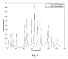
- Fig. 3 is a graph demonstrating the effectiveness of the de-permutation to improve smoothness of gradient terms across the frequency bins through a comparison between magnitudes of the gradient terms before and after the de-permutation;
- Fig. 4 is a flow chart illustrating an example method of performing convolutive blind source separation according to an embodiment of the present invention.
- Fig. 5 is a block diagram illustrating an exemplary system for implementing aspects of the present invention.
- aspects of the present invention may be embodied as a system, method or computer program product. Accordingly, aspects of the present invention may take the form of an entirely hardware embodiment, an entirely software embodiment (including firmware, resident software, microcode, etc.) or an embodiment combining software and hardware aspects that may all generally be referred to herein as a "circuit,” “module” or “system.” Furthermore, aspects of the present invention may take the form of a computer program product embodied in one or more computer readable medium(s) having computer readable program code embodied thereon.
- the computer readable medium may be a computer readable signal medium or a computer readable storage medium.
- a computer readable storage medium may be, for example, but not limited to, an electronic, magnetic, optical, electromagnetic, infrared, or semiconductor system, apparatus, or device, or any suitable combination of the foregoing.
- a computer readable storage medium may be any tangible medium that can contain, or store a program for use by or in connection with an instruction execution system, apparatus, or device.
- a computer readable signal medium may include a propagated data signal with computer readable program code embodied therein, for example, in baseband or as part of a carrier wave. Such a propagated signal may take any of a variety of forms, including, but not limited to, electro-magnetic, optical, or any suitable combination thereof.
- a computer readable signal medium may be any computer readable medium that is not a computer readable storage medium and that can communicate, propagate, or transport a program for use by or in connection with an instruction execution system, apparatus, or device.
- Program code embodied on a computer readable medium may be transmitted using any appropriate medium, including but not limited to wireless, wired line, optical fiber cable, RF, etc., or any suitable combination of the foregoing.
- Computer program code for carrying out operations for aspects of the present invention may be written in any combination of one or more programming languages, including an object oriented programming language such as Java, Smalltalk, C++ or the like and conventional procedural programming languages, such as the "C" programming language or similar programming languages.
- the program code may execute entirely on the user's computer, partly on the user's computer, as a stand-alone software package, partly on the user's computer and partly on a remote computer or entirely on the remote computer or server.
- the remote computer may be connected to the user's computer through any type of network, including a local area network (LAN) or a wide area network (WAN), or the connection may be made to an external computer (for example, through the Internet using an Internet Service Provider).
- LAN local area network
- WAN wide area network
- Internet Service Provider for example, AT&T, MCI, Sprint, EarthLink, MSN, GTE, etc.
- These computer program instructions may also be stored in a computer readable medium that can direct a computer, other programmable data processing apparatus, or other devices to function in a particular manner, such that the instructions stored in the computer readable medium produce an article of manufacture including instructions which implement the function/act specified in the flowchart and/or block diagram block or blocks.
- the computer program instructions may also be loaded onto a computer, other programmable data processing apparatus, or other devices to cause a series of operational steps to be performed on the computer, other programmable apparatus or other devices to produce a computer implemented process such that the instructions which execute on the computer or other programmable apparatus provide processes for implementing the functions/acts specified in the flowchart and/or block diagram block or blocks.
- Fig. 1 is a block diagram illustrating an example apparatus 100 for performing convolutive blind source separation according to an embodiment of the present invention.
- apparatus 100 includes a transformer 101, a calculator 102, an estimator 103 and a transformer 104.
- Sound sources 110-1 to 110-N emit sound signals S 1 to S N respectively.
- mixed signals of sound signals S 1 to S N are captured by microphones 130-1 to 130-N respectively.
- the captured signals are converted into digital signals s 1 to s N respectively.
- calculator 102 calculates values W ij ( ⁇ ) k, t ) of coefficients W ij ( ⁇ ,t ) of the unmixing filter W ( ⁇ k ,t ) by performing a gradient descent process on a cost function at least dependent on the coefficients W ij ( ⁇ ,t ) of the unmixing filter W ( ⁇ ,t ) .
- non-stationarity constraint To perform convolutive source separation, non-stationarity constraint is exploited. According to the non-stationarity constraint, it is possible to adopt a cost function f ( W ( ⁇ ,t )) to evaluate decorrelation between the estimated source signals Y i ( ⁇ , t ) ⁇ Y ( ⁇ , t ) . If each of the estimated source signals includes less mixed components, the cost function f ( W ( ⁇ ,t )) approaches a minimum value. Through a gradient descent process, it is possible to make the cost function f ( W ( ⁇ ,t )) approach the minimum value in an iterative manner.
- the gradient descent process is based on the observation that if a function f ( W ( ⁇ ,t )) is defined and differentiable in a neighborhood of a point W ( ⁇ ,t 0 ), then it decreases fastest if one goes in the direction of the negative gradient of f ( W ( ⁇ ,t )) at W ( ⁇ ,t 0 ) - ⁇ f ( W ( ⁇ , t 0 )) .
- E[ • ] denotes the statistical expectation
- W ( ⁇ ,t ) is a matrix where non-diagonal elements are coefficients and diagonal elements are assumed as unit gains
- R XX ( ⁇ , t ) is the cross-power spectrum of microphone signals.
- R xx ⁇ ⁇ t R x ⁇ 1 ⁇ x ⁇ 1 ⁇ ⁇ t R x ⁇ 1 ⁇ x ⁇ 2 ⁇ ⁇ t R x ⁇ 2 ⁇ x ⁇ 1 ⁇ ⁇ t R x ⁇ 2 ⁇ x ⁇ 2 ⁇ ⁇ t
- R xixj ( ⁇ ,t ) X i ( ⁇ ,t ) X j * ( ⁇ ,t ).
- ⁇ y ( ⁇ , t) is the diagonal component of an estimate of the sources' cross-power spectrum.
- its gradients with respect to the real and imaginary parts are obtained by taking partial derivatives formally with respect to the conjugate quantities W * ( ⁇ , t ).
- ⁇ ( ⁇ , t ) is the adaptation step size function that is made in inverse proportion to the input signal powers. Therefore, the gradient term is ⁇ ⁇ ⁇ t ⁇ ⁇ J t ⁇ W * ⁇ ⁇ t .
- gradients may be simplified as cross-power of two estimated source signals.
- the gradient for calculating the coefficient W 12 may be calculated as Y 2 * ( ⁇ , t ) Y 1 ( ⁇ , t ), and thus the corresponding gradient term is ⁇ 1 ⁇ ⁇ t ⁇ Y 2 * ⁇ ⁇ t ⁇ Y 1 ⁇ ⁇ t
- the gradient for calculating the coefficient W 21 may be calculated as Y 1 * ( ⁇ , t ) Y 2 ( ⁇ , t ), and thus the corresponding gradient term is ⁇ 2 ⁇ ⁇ t ⁇ Y 1 * ⁇ ⁇ t ⁇ Y 2 ⁇ ⁇ t
- ⁇ 1 ( ⁇ , t ) and ⁇ 2 ( ⁇ , t ) are the adaptation step size functions that are made in inverse proportion to the input signal powers.
- ⁇ ⁇ c E X 1 ⁇ 2 + E X 2 ⁇ 2 where c is a constant.
- the source signals in each frequency bin may be estimated with an arbitrary permutation. If the permutation is not consistent across the frequency bins, then converting the signal back to the time domain will combine contributions from different sources into a single channel
- calculator 102 adjusts the gradient terms ⁇ f ( W ij ( ⁇ 1 , t )) to ⁇ f ( W ij ( ⁇ M , t )) for calculating the values of the same coefficient W ij of the unmixing filters W ( ⁇ 1 ,t ) to W ( ⁇ M , t ) to improve smoothness of the gradient terms across the frequency bins ⁇ 1 to ⁇ M .
- the coefficients subjected to the adjustment may be some or all of the coefficients of the unmixing filters.
- the coefficients subjected to the adjustment may be non-diagonal coefficients of the unmixing filters.
- Various methods may be used to improve the smoothness of the gradient terms across the frequency bins by adjusting the gradient terms.
- each of the coefficients W ij ( ⁇ , t ) it is possible to transform the gradient terms ⁇ f ( W ij ( ⁇ il , t )) , ..., ⁇ f ( W ij ( ⁇ iM , t )) over the frequency bins ⁇ 1 to ⁇ M for calculating the values W ij ( ⁇ 1 , t ) to W ij ( ⁇ M , t ) of the coefficient W ij ( ⁇ , t ) into a time domain filter of length T, de-emphasize coefficients of the time domain filter at time indices t exceeding a threshold Q smaller than the length T, and transform coefficients of the time domain filter from time domain into frequency domain through a length-T transformation, so as to obtain adjusted gradient terms over the frequency bins ⁇ 1 to ⁇ M .
- De-emphasizing may be implemented by setting the coefficients to zero, or multiplying the coefficients with respective weights smaller than 1 (for example, 0.1), that is, reducing the coefficients at time indices t exceeding the threshold Q relative to coefficients of the time domain filter not at time indices t exceeding the threshold Q .
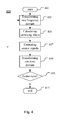
- Fig. 2 is a flow chart illustrating an example method 200 of adjusting gradient terms over frequency bins ⁇ 1 to ⁇ M for calculating a coefficient W ij .
- the method is implemented in Matlab, where the frequency domain gradient includes 129 frequency bins, and the size of Fast Fourier Transformation (FFT) and the time domain filter are 256.
- FFT Fast Fourier Transformation
- step 203 an array tmp is formed of gradient terms ⁇ f ( W ij ( ⁇ 1 , t )), ..., ⁇ f ( W ij ( ⁇ 129 , t )) (in array a ) and complex conjugates of gradient terms ⁇ f ( W ij ( ⁇ 128 , t )), ... , ⁇ f ( W ij ( ⁇ 2 , t )).
- Inverse FFT of size 256 is performed on array tmp to obtain a time domain filter of length 256, and an array at is formed of the coefficients of the time domain filter.
- coefficients in array at at time indices from Q+1 to T are set to zero.
- FFT of size 256 is performed on array at to obtain an array aa formed of 256 new coefficients.
- array a is updated with the first 129 coefficients of array aa.
- the method ends at step 213.
- Fig. 3 is a graph demonstrating the effectiveness of the de-permutation to improve smoothness of gradient terms across the frequency bins through a comparison between magnitudes of the gradient terms before and after the de-permutation. As illustrated in Fig. 3 , the magnitude before the de-permutation exhibits poor smoothness over frequency bins, and the magnitude after the de-permutation exhibits good smoothness over the frequency bins.
- calculator 102 provides unmixing filter W ( ⁇ ,t ) to estimator 103.
- estimator 103 estimates source signals Y ( ⁇ ,t ) by filtering the transformed input signals X ( ⁇ ,t ) through the respective unmixing filter W ( ⁇ ,t ) configured with the calculated values of the coefficients.
- the process of estimator 103 can be represented with Equation (1).
- Transformer 104 transforms the estimated source signals on the respective frequency bins into time domain, so as to produce separated source signals S' 1 to S' N .
- the de-permutation can be performed based on the gradient terms. This can be an alternative or addition to the de-permutation performed in other ways.
- calculator 102 may be further configured to adjust the threshold Q in at least one iteration of the gradient descent process.
- the at least one iteration may comprise arbitrary iteration, periodic iteration or every iteration.
- the threshold Q may be adjusted according to the proportion of the unmixing filters in a divergence condition. In this case, if the proportion in the current iteration is higher, or higher than that in the previous iteration, the threshold Q which is smaller or smaller than that in the previous iteration is adopted, and if the proportion in the current iteration is lower, or lower than that in the previous iteration, the threshold Q which is greater or greater than that in the previous iteration is adopted.
- the divergence condition may be determined based on whether the unmixing filter is stable. In an example, the divergence condition of the unmixing filter corresponding to the respective frequency bin is determined if the power ratio of the output to the input of the unmixing filter is greater than a threshold D.
- 2 or Ratio E Y 1 2 + E
- the threshold D may be determined according to the requirement on the smoothness of the gradient terms. The higher requirement determines the smaller threshold D, and the lower requirement determines the greater threshold D. For example, the threshold D is equal to or smaller than 1.
- the threshold Q may be adjusted according to the smoothness of the gradient terms between the frequency bins.
- the threshold Q is increased, e.g. to 2Q or the maximum length allowed if the smoothness is equal to or higher than a threshold P, and is reduced, e.g. to Q/2 if the smoothness is lower than the threshold P.
- Various measures may be used to evaluate the smoothness. For example, it is possible to calculate correlations of gradient terms between neighboring frequency bins and then average the correlations as the smoothness.
- the threshold P may be determined according to the requirement on the smoothness of the gradient terms. The higher requirement determines the higher threshold P, and the lower requirement determines the lower threshold P. In an example, the threshold P is equal to or greater than 0.5.
- the threshold Q may be adjusted according to the consistency of the spectrum of the estimated source signals.
- the threshold Q is increased, e.g. to 2Q or the maximum length allowed if the consistency is equal to or higher than a threshold G, and is reduced, e.g. to Q/2 if the consistency is lower than the threshold G.
- Various measures may be used to evaluate the consistency of the spectrum of the estimated source signals. For example, it is possible to calculate correlations of the estimated source signals between neighboring frequency bins and average the correlations as the consistency of the spectrum of the estimated source signals.
- the threshold G may be determined according to the requirement on the consistency of the spectrum. The higher requirement determines the higher threshold G, and the lower requirement determines the lower threshold G. In an example, the threshold G is equal to or greater than 0.5.
- calculator 102 may be further configured to adjust the gradient terms by choosing the permutation that minimizes the Euclidean distances or maximizes correlations of gradient terms between neighboring frequency bins. In this case, it is possible to try arbitrary permutations of the gradient terms and choose the permutation that minimizes the Euclidean distances or maximizes correlations of gradient terms between neighboring frequency bins. The Euclidean distances or correlations may be evaluated with their total sum or average.
- calculator 102 may be further configured to determine whether the unmixing filter corresponding to each of the frequency bins is in a divergence condition or not.
- the divergence condition may be determined based on whether the unmixing filter is stable. In an example, the divergence condition of the unmixing filter corresponding to the respective frequency bin is determined if the power ratio of the output to the input of the unmixing filter is greater than the threshold D.
- Calculator 102 may be further configured to adopt the gradient terms calculated in the previous iteration as the gradient terms for use in the current iteration if the unmixing filter is in the divergence condition, and calculate the gradient terms for use in the current iteration if the unmixing filter is not in the divergence condition.
- previous gradient terms are used for a particular frequency bin if the corresponding unmixing filter is deemed unstable, or new gradient terms are calculated if otherwise. Then the gradient terms are subjected to de-permutation. From Eqs. (5) and (6), it can be seen that such an approach may achieve a balance between maintaining existing filters (previously regularized) and adapting to the new gradient direction.
- the calculating cost may be reduced. Further, by calculating the gradient terms based on Eqs. (10) and (11), the system can be simple, efficient and stable.
- Fig. 4 is a flow chart illustrating an example method 400 of performing convolutive blind source separation according to an embodiment of the present invention.
- step 403 digital signals s 1 to s N obtained through respective microphones are transformed into frequency domain respectively.
- values W ij ( ⁇ k ,t ) of coefficients W ij ( ⁇ ,t ) of the unmixing filter W ( ⁇ k ,t ) are calculated by performing a gradient descent process on a cost function at least dependent on the coefficients W ij ( ⁇ ,t ) of the unmixing filter W ( ⁇ ,t ).
- non-stationarity constraint To perform convolutive source separation, non-stationarity constraint is exploited. According to the non-stationarity constraint, it is possible to adopt a cost function f ( W ( ⁇ ,t )) to evaluate decorrelation between the estimated source signals Y i ( ⁇ , t ) ⁇ Y ( ⁇ ,t ) . If each of the estimated source signals includes less mixed components, the cost function f ( W ( ⁇ ,t )) approaches a minimum value. Through a gradient descent process, it is possible to make the cost function f ( W ( ⁇ ,t )) approach the minimum value in an iterative manner.
- second-order statistics in the frequency domain is captured by the cross-power spectrum in Eq. (5).
- the goal is to minimize the cross-powers on the off-diagonal of this matrix, e.g. by minimizing the cost function in Eq. (7).
- its gradients with respect to the real and imaginary parts are obtained by taking partial derivatives formally with respect to the conjugate quantities W *( ⁇ ,t ) .
- the gradient at time t is estimated as in Eq. (8) and the unmixing filter is estimated as in Eq. (9).
- the gradients may be simplified as cross-power of two estimated source signals.
- the gradient term for calculating the coefficient W 12 may be calculated based on Eq. (10)
- the gradient term for calculating the coefficient W 21 may be calculated based on Eq. (11).
- the gradient terms ⁇ f ( W ij ( ⁇ 1 , t )) to ⁇ f ( W ij ( ⁇ M , t )) for calculating the values of the same coefficient W ij of the unmixing filters W ( ⁇ 1 ,t ) to W ( ⁇ M ,t ) are adjusted to improve smoothness of the gradient terms across the frequency bins ⁇ 1 to ⁇ M .
- the coefficients subjected to the adjustment may be some or all of the coefficients of the unmixing filters.
- the coefficients subjected to the adjustment may be non-diagonal coefficients of the unmixing filters.
- Various methods may be used to improve the smoothness of the gradient terms across the frequency bins by adjusting the gradient terms.
- each of the coefficients W ij ( ⁇ ,t ) it is possible to transform the gradient terms ⁇ f ( W ij ( ⁇ il , t )) , ..., ⁇ f ( W ij ( ⁇ iM , t )) over the frequency bins ⁇ 1 to ⁇ M for calculating the values W ij ( ⁇ 1 , t ) to W ij ( ⁇ M , t ) of the coefficient W ij ( ⁇ ,t ) into a time domain filter of length T, de-emphasize coefficients of the time domain filter at time indices t exceeding a threshold Q smaller than the length T, and transform coefficients of the time domain filter from time domain into frequency domain through a length-T transformation, so as to obtain adjusted gradient terms over the frequency bins ⁇ 1 to ⁇ M .
- De-emphasizing may be implemented by setting the coefficients to zero, or multiplying the coefficients with respective weights smaller than 1 (for example, 0.1), that is, reducing the coefficients at time indices t exceeding the threshold Q relative to coefficients of the time domain filter not at time indices t exceeding the threshold Q .
- the unmixing filter W ( ⁇ ,t ) obtained at step 405 is used at step 407.
- source signals Y ( ⁇ ,t ) are estimated by filtering the transformed input signals X ( ⁇ ,t ) through the respective unmixing filter W ( ⁇ ,t ) configured with the calculated values of the coefficients.
- the process of step 407 can be represented with Equation (1).
- the estimated source signals on the respective frequency bins are transformed into time domain, so as to produce separated source signals S' 1 to S' N .
- step 411 it is determined whether there are other digital signals to be processed. If YES, the process returns to step 403. If NO, method 400 ends at step 413.
- step 405 may further comprise adjusting the threshold Q in at least one iteration of the gradient descent process.
- the at least one iteration may comprises arbitrary iteration, periodic iteration or every iteration.
- the threshold Q may be adjusted according to the proportion of the unmixing filters in a divergence condition. In this case, if the proportion in the current iteration is higher, or higher than that in the previous iteration, the threshold Q which is smaller or smaller than that in the previous iteration is adopted, and if the proportion in the current iteration is lower, or lower than that in the previous iteration, the threshold Q which is greater or greater than that in the previous iteration is adopted.
- the divergence condition may be determined based on whether the unmixing filter is stable. In an example, the divergence condition of the unmixing filter corresponding to the respective frequency bin is determined if the power ratio of the output to the input of the unmixing filter is greater than a threshold D.
- the threshold D may be determined according to the requirement on the smoothness of the gradient terms. The higher requirement determines the smaller threshold D, and the lower requirement determines the greater threshold D. For example, the threshold D is equal to or smaller than 1.
- the threshold Q may be adjusted according to the smoothness of the gradient terms between the frequency bins.
- the threshold Q is increased, e.g. to 2Q or the maximum length allowed if the smoothness is equal to or higher than a threshold P, and is reduced, e.g. to Q/2 if the smoothness is lower than the threshold P.
- Various measures may be used to evaluate the smoothness. For example, it is possible to calculate correlations of gradient terms between neighboring frequency bins and then average the correlations as the smoothness.
- the threshold P may be determined according to the requirement on the smoothness of the gradient terms. The higher requirement determines the higher threshold P, and the lower requirement determines the lower threshold P. In an example, the threshold P is equal to or greater than 0.5.
- the threshold Q may be adjusted according to the consistency of the spectrum of the estimated source signals.
- the threshold Q is increased, e.g. to 2Q or the maximum length allowed if the consistency is equal to or higher than a threshold G, and is reduced, e.g. to Q/2 if the consistency is lower than the threshold G.
- Various measures may be used to evaluate the consistency of the spectrum of the estimated source signals. For example, it is possible to calculate correlations of the estimated source signals between neighboring frequency bins and average the correlations as the consistency of the spectrum of the estimated source signals.
- the threshold G may be determined according to the requirement on the consistency of the spectrum. The higher requirement determines the higher threshold G, and the lower requirement determines the lower threshold G. In an example, the threshold G is equal to or greater than 0.5.
- step 405 may further comprise adjusting the gradient terms by choosing the permutation that minimizes the Euclidean distances or maximizes correlations of gradient terms between neighboring frequency bins.
- the Euclidean distances or correlations may be evaluated with their total sum or average.
- step 405 may further comprise determining whether the unmixing filter corresponding to each of the frequency bins is in a divergence condition or not.
- the divergence condition may be determined based on whether the unmixing filter is stable. In an example, the divergence condition of the unmixing filter corresponding to the respective frequency bin is determined if the power ratio of the output to the input of the unmixing filter is greater than the threshold D.
- step 405 may further comprise adopting the gradient terms calculated in the previous iteration as the gradient terms for use in the current iteration if the unmixing filter is in the divergence condition, and calculating the gradient terms for use in the current iteration if the unmixing filter is not in the divergence condition.
- previous gradient terms are used for a particular frequency bin if the corresponding unmixing filter is deemed unstable, or new gradient terms are calculated if otherwise. Then the gradient terms are subjected to de-permutation. From Eqs. (5) and (6), it can be seen that such an approach may achieve a balance between maintaining existing filters (previously regularized) and adapting to the new gradient direction.
- step 405 may further comprise, with respect to each of the frequency bins ⁇ , calculating the gradient terms for use in the current iteration according to Eqs. (15) and (16), or according to Eqs. (17) and (18), or according to Eqs. (19) and (20).
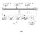
- Fig. 5 is a block diagram illustrating an exemplary system for implementing the aspects of the present invention.
- a central processing unit (CPU) 501 performs various processes in accordance with a program stored in a read only memory (ROM) 502 or a program loaded from a storage section 508 to a random access memory (RAM) 503.
- ROM read only memory
- RAM random access memory
- data required when the CPU 501 performs the various processes or the like is also stored as required.
- the CPU 501, the ROM 502 and the RAM 503 are connected to one another via a bus 504.
- An input / output interface 505 is also connected to the bus 504.
- the following components are connected to the input / output interface 505: an input section 506 including a keyboard, a mouse, or the like ; an output section 507 including a display such as a cathode ray tube (CRT), a liquid crystal display (LCD), or the like, and a loudspeaker or the like; the storage section 508 including a hard disk or the like ; and a communication section 509 including a network interface card such as a LAN card, a modem, or the like.
- the communication section 509 performs a communication process via the network such as the internet.
- a drive 510 is also connected to the input / output interface 505 as required.
- a removable medium 511 such as a magnetic disk, an optical disk, a magneto - optical disk, a semiconductor memory, or the like, is mounted on the drive 510 as required, so that a computer program read therefrom is installed into the storage section 508 as required.
- the program that constitutes the software is installed from the network such as the internet or the storage medium such as the removable medium 511.
- a method of performing convolutive blind source separation comprising:
- EE 7 The method according to EE6, wherein the de-emphasizing of the coefficients comprises zeroing the coefficients at time indices exceeding the first threshold, or reducing the coefficients at time indices exceeding the first threshold relative to coefficients of the time domain filter not at time indices exceeding the first threshold.
- EE 8 The method according to EE6, wherein the first threshold is adjusted in at least one iteration of the gradient descent process according to the proportion of the unmixing filters in a divergence condition, where the higher the proportion is, the smaller the first threshold is.
- EE 9 The method according to EE6, wherein the first threshold is adjusted in at least one iteration of the gradient descent process according to the smoothness, where the first threshold is increased if the smoothness is equal to or higher than a second threshold, and is reduced if the smoothness is lower than the second threshold.
- EE 10 The method according to EE9, wherein the smoothness is evaluated by calculating correlations of gradient terms between neighboring frequency bins and then averaging the correlations.
- EE 12 The method according to EE6, wherein the first threshold is adjusted in at least one iteration of the gradient descent process according to consistency of the spectrum of the estimated source signals, where the first threshold is increased if the consistency is equal to or higher than a third threshold, and is reduced if the consistency is lower than the third threshold.
- EE 13 The method according to EE11, wherein the consistency is evaluated by calculating correlations of the estimated source signals between neighboring frequency bins and averaging the correlations.
- EE 15 The method according to EE5 or 8, wherein the divergence condition of the unmixing filter is determined if the power ratio of the output to the input of the unmixing filter is greater than a fourth threshold.
- EE 17 The method according to EE1, wherein the gradient terms are adjusted by choosing one of permutations that minimizes the Euclidean distances or maximizes correlations of gradient terms between neighboring frequency bins.
- An apparatus for performing convolutive blind source separation comprising:
- EE 22 The apparatus according to EE18, wherein the calculator is further configured to, with respect to each of the frequency bins, determine whether the unmixing filter is in a divergence condition or not, adopt the gradient terms calculated in the previous iteration as the gradient terms for use in the current iteration if the unmixing filter is in the divergence condition, and calculate the gradient terms for use in the current iteration if the unmixing filter is not in the divergence condition.
- EE 23 The apparatus according to EE18, wherein the calculator is configured to, with respect to each of the coefficients, transform the gradient terms over the frequency bins for calculating the coefficient into a time domain filter of length T, de-emphasize coefficients of the time domain filter at time indices exceeding a first threshold smaller than the length T, and transform coefficients of the time domain filter from time domain into frequency domain through a length-T transformation.
- EE 24 The apparatus according to EE23, wherein the de-emphasizing of the coefficients comprises zeroing the coefficients at time indices exceeding the first threshold, or reducing the coefficients at time indices exceeding the first threshold relative to coefficients of the time domain filter not at time indices exceeding the first threshold.
- EE 25 The apparatus according to EE23, wherein the calculator is further configured to adjust the first threshold in at least one iteration of the gradient descent process according to the proportion of the unmixing filters in a divergence condition, where the higher the proportion is, the smaller the first threshold is.
- EE 26 The apparatus according to EE23, wherein the calculator is further configured to adjust the first threshold in at least one iteration of the gradient descent process according to the smoothness, where the first threshold is increased if the smoothness is equal to or higher than a second threshold, and is reduced if the smoothness is lower than the second threshold.
- EE 27 The apparatus according to EE26, wherein the smoothness is evaluated by calculating correlations of gradient terms between neighboring frequency bins and then averaging the correlations.
- EE 28 The apparatus according to EE27, wherein the second threshold is equal to or greater than 0.5.
- EE 29 The apparatus according to EE23, wherein the calculator is further configured to adjust the first threshold in at least one iteration of the gradient descent process according to consistency of the spectrum of the estimated source signals, where the first threshold is increased if the consistency is equal to or higher than a third threshold, and is reduced if the consistency is lower than the third threshold.
- EE 30 The apparatus according to EE29, wherein the consistency is evaluated by calculating correlations of the estimated source signals between neighboring frequency bins and averaging the correlations.
- EE 32 The apparatus according to EE22 or 25, wherein the divergence condition of the unmixing filter is determined if the power ratio of the output to the input of the unmixing filter is greater than a fourth threshold.
- EE 34 The apparatus according to EE18, wherein the calculator is further configured to adjust the gradient terms by choosing one of permutations that minimizes the Euclidean distances or maximizes correlations of gradient terms between neighboring frequency bins.
- a computer-readable medium having computer program instructions recorded thereon, when being executed by a processor, the instructions enabling the processor to perform a method of convolutive blind source separation based on second order statistics comprising:
Landscapes
- Engineering & Computer Science (AREA)
- Computer Vision & Pattern Recognition (AREA)
- Data Mining & Analysis (AREA)
- Theoretical Computer Science (AREA)
- Physics & Mathematics (AREA)
- Bioinformatics & Computational Biology (AREA)
- Bioinformatics & Cheminformatics (AREA)
- Evolutionary Biology (AREA)
- Evolutionary Computation (AREA)
- Artificial Intelligence (AREA)
- General Engineering & Computer Science (AREA)
- General Physics & Mathematics (AREA)
- Life Sciences & Earth Sciences (AREA)
- Quality & Reliability (AREA)
- Computational Linguistics (AREA)
- Signal Processing (AREA)
- Health & Medical Sciences (AREA)
- Audiology, Speech & Language Pathology (AREA)
- Human Computer Interaction (AREA)
- Acoustics & Sound (AREA)
- Multimedia (AREA)
- Compression, Expansion, Code Conversion, And Decoders (AREA)
- Circuit For Audible Band Transducer (AREA)
- Measurement And Recording Of Electrical Phenomena And Electrical Characteristics Of The Living Body (AREA)
- Complex Calculations (AREA)
Abstract
Description
- The present invention relates generally to audio signal processing. More specifically, embodiments of the present invention relate to methods and apparatuses for convolutive blind source separation.
- In various real-world applications, a convolutive mixing model is usually used to approximate the relationships between the original source signals and the mixed signals captured by the sensors such as microphones. A linear convolution can be approximated by a circular convolution if the frame size of the discrete Fourier transform (DFT) is much larger than the channel length. Then a convolutive mixing process can be represented as multiplication in the frequency domain

where Y(ω,t) represents the estimated sources [Y1(ω,t),..., YN(ω,t)]T, X(ω,t) is the microphone signals [X1(ω,t),..., XN(ω,t)]T, and W(ω,t) (also called as unmixing filter for frequency bin ω) denotes the unmixing matrix including unmixing filter coefficients. - For example, in a two-input-two-output (TITO) case, by assuming a unit gain for direct channels, the unmixing matrix can be represented as

- Then the separated signals can be represented as


- Various approaches have been proposed to estimate the unmixing filters. One class of algorithms obtain separation based on second order statistics (SOS) by requiring only non-correlated sources rather than the stronger condition of independence. By exploring additional constraints such as non-stationarity, sufficient conditions for separation can be achieved for SOS systems. One SOS-based approach is the so-called adaptive decorrelation filter (ADF) formulation, which is based on the classical adaptive noise cancellation (ANC) scheme. (See E. Weinstein, M. Feder, and A. V. Oppenheim, "Multi-channel signal separation by decorrelation," IEEE Trans. Speech Audio Processing, vol. 1, pp. 405--413, Apr. 1993) Other SOS-based approaches have also been proposed, where a cost function for evaluating the decorrelation between separated signals is defined, and values of coefficients of unmixing filters are calculated adaptively by performing a gradient descent process on the cost function. (See Parra L., Spence C., "Convolutive blind source separation of non-stationary sources", IEEE Trans. on Speech and Audio Processing pp. 320-327, May 2000.)
- According to an embodiment of the present invention, a method of performing convolutive blind source separation is provided. Each of a plurality of input signals is transformed into frequency domain. Values of coefficients of unmixing filters corresponding to frequency bins are calculated by performing a gradient descent process on a cost function at least dependent on the coefficients of the unmixing filters. In each iteration of the gradient descent process, gradient terms for calculating the values of the same coefficient of the unmixing filters are adjusted to improve smoothness of the gradient terms across the frequency bins. With respect to each of the frequency bins, source signals are estimated by filtering the transformed input signals through the respective unmixing filter configured with the calculated values of the coefficients. The estimated source signals on the respective frequency bins are transformed into time domain. The cost function is adapted to evaluate decorrelation between the estimated source signals.
- According to an embodiment of the present invention, an apparatus for performing convolutive blind source separation is provided. The apparatus includes a first transformer, a calculator, an estimator and a second transformer. The first transformer transforms each of a plurality of input signals into frequency domain. The calculator calculates values of coefficients of unmixing filters corresponding to frequency bins by performing a gradient descent process on a cost function at least dependent on the coefficients of the unmixing filters. In each iteration of the gradient descent process, gradient terms for calculating the values of the same coefficient of the unmixing filter are adjusted to improve smoothness of the gradient terms across the frequency bins. With respect to each of the frequency bins, the estimator estimates source signals by filtering the transformed input signals through the respective unmixing filter configured with the calculated values of the coefficients. The second transformer transforms the estimated source signals on the respective frequency bins into time domain. The cost function is adapted to evaluate decorrelation between the estimated source signals.
- According to an embodiment of the present invention, a computer-readable medium having computer program instructions recorded thereon is provided. When being executed by a processor, the instructions enable the processor to perform a method of performing convolutive blind source separation. According to the method, each of a plurality of input signals is transformed into frequency domain. Values of coefficients of unmixing filters corresponding to frequency bins are calculated by performing a gradient descent process on a cost function at least dependent on the coefficients of the unmixing filters. In each iteration of the gradient descent process, gradient terms for calculating the values of the same coefficient of the unmixing filters are adjusted to improve smoothness of the gradient terms across the frequency bins. With respect to each of the frequency bins, source signals are estimated by filtering the transformed input signals through the respective unmixing filter configured with the calculated values of the coefficients. The estimated source signals on the respective frequency bins are transformed into time domain. The cost function is adapted to evaluate decorrelation between the estimated source signals.
- The present invention is illustrated by way of examples, and not by way of limitation, in the figures of the accompanying drawings and in which like reference numerals refer to similar elements and in which:
-
Fig. 1 is a block diagram illustrating an example apparatus for performing convolutive blind source separation according to an embodiment of the present invention; -
Fig. 2 is a flow chart illustrating an example method of adjusting gradient terms over frequency bins for calculating a coefficient; -
Fig. 3 is a graph demonstrating the effectiveness of the de-permutation to improve smoothness of gradient terms across the frequency bins through a comparison between magnitudes of the gradient terms before and after the de-permutation; -
Fig. 4 is a flow chart illustrating an example method of performing convolutive blind source separation according to an embodiment of the present invention; and -
Fig. 5 is a block diagram illustrating an exemplary system for implementing aspects of the present invention. - The embodiments of the present invention are below described by referring to the drawings. It is to be noted that, for purpose of clarity, representations and descriptions about those components and processes known by those skilled in the art but unrelated to the present invention are omitted in the drawings and the description.
- As will be appreciated by one skilled in the art, aspects of the present invention may be embodied as a system, method or computer program product. Accordingly, aspects of the present invention may take the form of an entirely hardware embodiment, an entirely software embodiment (including firmware, resident software, microcode, etc.) or an embodiment combining software and hardware aspects that may all generally be referred to herein as a "circuit," "module" or "system." Furthermore, aspects of the present invention may take the form of a computer program product embodied in one or more computer readable medium(s) having computer readable program code embodied thereon.
- Any combination of one or more computer readable medium(s) may be utilized. The computer readable medium may be a computer readable signal medium or a computer readable storage medium. A computer readable storage medium may be, for example, but not limited to, an electronic, magnetic, optical, electromagnetic, infrared, or semiconductor system, apparatus, or device, or any suitable combination of the foregoing. More specific examples (a non-exhaustive list) of the computer readable storage medium would include the following: an electrical connection having one or more wires, a portable computer diskette, a hard disk, a random access memory (RAM), a read-only memory (ROM), an erasable programmable read-only memory (EPROM or Flash memory), an optical fiber, a portable compact disc read-only memory (CD-ROM), an optical storage device, a magnetic storage device, or any suitable combination of the foregoing. In the context of this document, a computer readable storage medium may be any tangible medium that can contain, or store a program for use by or in connection with an instruction execution system, apparatus, or device.
- A computer readable signal medium may include a propagated data signal with computer readable program code embodied therein, for example, in baseband or as part of a carrier wave. Such a propagated signal may take any of a variety of forms, including, but not limited to, electro-magnetic, optical, or any suitable combination thereof.
- A computer readable signal medium may be any computer readable medium that is not a computer readable storage medium and that can communicate, propagate, or transport a program for use by or in connection with an instruction execution system, apparatus, or device.
- Program code embodied on a computer readable medium may be transmitted using any appropriate medium, including but not limited to wireless, wired line, optical fiber cable, RF, etc., or any suitable combination of the foregoing.
- Computer program code for carrying out operations for aspects of the present invention may be written in any combination of one or more programming languages, including an object oriented programming language such as Java, Smalltalk, C++ or the like and conventional procedural programming languages, such as the "C" programming language or similar programming languages. The program code may execute entirely on the user's computer, partly on the user's computer, as a stand-alone software package, partly on the user's computer and partly on a remote computer or entirely on the remote computer or server. In the latter scenario, the remote computer may be connected to the user's computer through any type of network, including a local area network (LAN) or a wide area network (WAN), or the connection may be made to an external computer (for example, through the Internet using an Internet Service Provider).
- Aspects of the present invention are described below with reference to flowchart illustrations and/or block diagrams of methods, apparatus (systems) and computer program products according to embodiments of the invention. It will be understood that each block of the flowchart illustrations and/or block diagrams, and combinations of blocks in the flowchart illustrations and/or block diagrams, can be implemented by computer program instructions. These computer program instructions may be provided to a processor of a general purpose computer, special purpose computer, or other programmable data processing apparatus to produce a machine, such that the instructions, which execute via the processor of the computer or other programmable data processing apparatus, create means for implementing the functions/acts specified in the flowchart and/or block diagram block or blocks.
- These computer program instructions may also be stored in a computer readable medium that can direct a computer, other programmable data processing apparatus, or other devices to function in a particular manner, such that the instructions stored in the computer readable medium produce an article of manufacture including instructions which implement the function/act specified in the flowchart and/or block diagram block or blocks.
- The computer program instructions may also be loaded onto a computer, other programmable data processing apparatus, or other devices to cause a series of operational steps to be performed on the computer, other programmable apparatus or other devices to produce a computer implemented process such that the instructions which execute on the computer or other programmable apparatus provide processes for implementing the functions/acts specified in the flowchart and/or block diagram block or blocks.
-
Fig. 1 is a block diagram illustrating anexample apparatus 100 for performing convolutive blind source separation according to an embodiment of the present invention. - As illustrated in
Fig. 1 ,apparatus 100 includes atransformer 101, acalculator 102, anestimator 103 and atransformer 104. - Sound sources 110-1 to 110-N emit sound signals S 1 to SN respectively. Through respective
convolutive channels 120, mixed signals of sound signals S 1 to SN are captured by microphones 130-1 to 130-N respectively. The captured signals are converted into digital signals s 1 to sN respectively. -
Transformer 101 transforms digital signals s 1 to s N into frequency domain respectively. For example, from each digital signal s i,transformer 101 may obtain a frame corresponding to time period from t to t+T, and convert the frame into frequency domain. Therefore, signals X (ω,t) is obtained, where X (ω,t)= [X 1(ω,t),..., X N(ω,t)]T , and ω represents any one of frequency bins ω1 to ωM. By repeating in this way, for each digital signal s i,transformer 101 may transform a series of frames into frequency domain. - With respect to each unmixing filter W (ωk,t) of unmixing filters W (ω1,t) to W (ωM,t) corresponding to respective frequency bins ω1 to ωM,
calculator 102 calculates values W ij(ω)k, t) of coefficients W ij(ω,t) of the unmixing filter W (ωk ,t) by performing a gradient descent process on a cost function at least dependent on the coefficients W ij(ω,t) of the unmixing filter W (ω,t). - To perform convolutive source separation, non-stationarity constraint is exploited. According to the non-stationarity constraint, it is possible to adopt a cost function f( W (ω,t)) to evaluate decorrelation between the estimated source signals Y i(ω,t)∈ Y (ω,t). If each of the estimated source signals includes less mixed components, the cost function f( W (ω,t)) approaches a minimum value. Through a gradient descent process, it is possible to make the cost function f( W (ω,t)) approach the minimum value in an iterative manner.
- The gradient descent process is based on the observation that if a function f( W (ω,t)) is defined and differentiable in a neighborhood of a point W (ω,t0 ), then it decreases fastest if one goes in the direction of the negative gradient of f( W (ω,t)) at W (ω,t0 )- ∇f( W (ω, t0 )). It follows that, if W (ω,t 1)= W (ω,t0 )-µ∇f( W (ω, t0 )) for µ > 0 a small enough number (also called as a step size), then f( W (ω, t0 ))≥f( W (ω, t 1)). In the following, the term µ∇f( W (ω, ti ) is also called as a gradient term, which is the product of the step size µ and the gradient ∇f( W (ω, ti ). With this observation, it is possible to start with a guess W (ω,t0 ) for a local minimum of f( W (ω,t)), and considers the sequence W (ω,t0 ), W (ω,t 1), W (ω,t 2), ... such that W (ω,t n+1)= W (ω,tn )- µ n ∇f( W (ω, tn )), n≥0. It is possible to obtain f( W (ω, t0 ))≥f( W (ω, t 1)) ≥f( W (ω, t 2)) ≥ ..., so hopefully the process converges to the desired local minimum.
- For example, second-order statistics in the frequency domain is captured by the cross-power spectrum,

where E[ • ] denotes the statistical expectation, W (ω,t) is a matrix where non-diagonal elements are coefficients and diagonal elements are assumed as unit gains, and R XX (ω, t) is the cross-power spectrum of microphone signals. For example, in the TITO case,
where Rxixj (ω,t)=Xi (ω,t)Xj * (ω,t). - The goal is to minimize the cross-powers on the off-diagonal of this matrix, e.g. by minimizing the cost function:

where Λy(ω, t) is the diagonal component of an estimate of the sources' cross-power spectrum. In this case, its gradients with respect to the real and imaginary parts are obtained by taking partial derivatives formally with respect to the conjugate quantities W*(ω,t). Thus the gradient at time t is
and the unmixing filter is estimated as
where µ(ω, t) is the adaptation step size function that is made in inverse proportion to the input signal powers. Therefore, the gradient term is
- For another example, in the TITO case, gradients may be simplified as cross-power of two estimated source signals. For example, the gradient for calculating the coefficient W 12 may be calculated as Y 2 * (ω, t)Y 1(ω, t), and thus the corresponding gradient term is

The gradient for calculating the coefficient W 21 may be calculated as Y 1 *(ω, t)Y 2(ω, t), and thus the corresponding gradient term is
where µ1(ω, t) and µ2(ω, t) are the adaptation step size functions that are made in inverse proportion to the input signal powers. For example,
where c is a constant. - In this way, for each non-diagonal elements (coefficients W ij(ω,t), i≠j) of the unmixing filter W (ω,t), a gradient descent process is performed.
- If the convolutive problem is treated for each frequency bin as a separate problem, the source signals in each frequency bin may be estimated with an arbitrary permutation. If the permutation is not consistent across the frequency bins, then converting the signal back to the time domain will combine contributions from different sources into a single channel
- It is possible to solve the permutation problem (de-permutation) by putting a consistency (smoothness) constraint on gradient terms across the frequency bins. In each iteration of the gradient descent process, that is, for each time t,
calculator 102 adjusts the gradient terms µ∇f(W ij(ω1, t)) to µ∇f(W ij(ωM, t)) for calculating the values of the same coefficient W ij of the unmixing filters W (ω1 ,t) to W (ωM,t) to improve smoothness of the gradient terms across the frequency bins ω1 to ωM. The coefficients subjected to the adjustment may be some or all of the coefficients of the unmixing filters. For example, the coefficients subjected to the adjustment may be non-diagonal coefficients of the unmixing filters. - Various methods may be used to improve the smoothness of the gradient terms across the frequency bins by adjusting the gradient terms.
- In an example, with respect to each of the coefficients W ij(ω,t), it is possible to transform the gradient terms µ∇f(W ij(ωil, t)), ..., µ∇f(W ij(ωiM, t)) over the frequency bins ω1 to ωM for calculating the values W ij(ω1 , t) to W ij(ωM , t) of the coefficient W ij(ω,t) into a time domain filter of length T, de-emphasize coefficients of the time domain filter at time indices t exceeding a threshold Q smaller than the length T, and transform coefficients of the time domain filter from time domain into frequency domain through a length-T transformation, so as to obtain adjusted gradient terms over the frequency bins ω1 to ωM. De-emphasizing may be implemented by setting the coefficients to zero, or multiplying the coefficients with respective weights smaller than 1 (for example, 0.1), that is, reducing the coefficients at time indices t exceeding the threshold Q relative to coefficients of the time domain filter not at time indices t exceeding the threshold Q.
-
Fig. 2 is a flow chart illustrating anexample method 200 of adjusting gradient terms over frequency bins ω1 to ωM for calculating a coefficient W ij. In this example, the method is implemented in Matlab, where the frequency domain gradient includes 129 frequency bins, and the size of Fast Fourier Transformation (FFT) and the time domain filter are 256. - As illustrated in
Fig. 2 ,method 200 starts fromstep 201. Atstep 203, an array tmp is formed of gradient terms µ∇f(W ij(ω1 , t)), ..., µ∇f(W ij(ω 129, t)) (in array a) and complex conjugates of gradient terms µ∇f(W ij(ω128 , t)), ...,µ∇f(W ij(ω 2, t)). - At
step 205, Inverse FFT of size 256 is performed on array tmp to obtain a time domain filter of length 256, and an array at is formed of the coefficients of the time domain filter. - At
step 207, coefficients in array at at time indices from Q+1 to T are set to zero. - At
step 209, FFT of size 256 is performed on array at to obtain an array aa formed of 256 new coefficients. - At
step 211, array a is updated with the first 129 coefficients of array aa. - The method ends at
step 213. -
Fig. 3 is a graph demonstrating the effectiveness of the de-permutation to improve smoothness of gradient terms across the frequency bins through a comparison between magnitudes of the gradient terms before and after the de-permutation. As illustrated inFig. 3 , the magnitude before the de-permutation exhibits poor smoothness over frequency bins, and the magnitude after the de-permutation exhibits good smoothness over the frequency bins. - Returning to
Fig. 1 ,calculator 102 provides unmixing filter W (ω,t) toestimator 103. With respect to each of the frequency bins,estimator 103 estimates source signals Y (ω,t) by filtering the transformed input signals X (ω,t) through the respective unmixing filter W (ω,t) configured with the calculated values of the coefficients. The process ofestimator 103 can be represented with Equation (1). -
Transformer 104 transforms the estimated source signals on the respective frequency bins into time domain, so as to produce separated source signals S'1 to S'N. - According to the embodiments, the de-permutation can be performed based on the gradient terms. This can be an alternative or addition to the de-permutation performed in other ways.
- In a further embodiment of
apparatus 100,calculator 102 may be further configured to adjust the threshold Q in at least one iteration of the gradient descent process. The at least one iteration may comprise arbitrary iteration, periodic iteration or every iteration. - In an example, the threshold Q may be adjusted according to the proportion of the unmixing filters in a divergence condition. In this case, if the proportion in the current iteration is higher, or higher than that in the previous iteration, the threshold Q which is smaller or smaller than that in the previous iteration is adopted, and if the proportion in the current iteration is lower, or lower than that in the previous iteration, the threshold Q which is greater or greater than that in the previous iteration is adopted. The divergence condition may be determined based on whether the unmixing filter is stable. In an example, the divergence condition of the unmixing filter corresponding to the respective frequency bin is determined if the power ratio of the output to the input of the unmixing filter is greater than a threshold D.
- As an example, the power ratio Ratio may be represented as

or
- The threshold D may be determined according to the requirement on the smoothness of the gradient terms. The higher requirement determines the smaller threshold D, and the lower requirement determines the greater threshold D. For example, the threshold D is equal to or smaller than 1.
- In another example, the threshold Q may be adjusted according to the smoothness of the gradient terms between the frequency bins. In this case, the threshold Q is increased, e.g. to 2Q or the maximum length allowed if the smoothness is equal to or higher than a threshold P, and is reduced, e.g. to Q/2 if the smoothness is lower than the threshold P. Various measures may be used to evaluate the smoothness. For example, it is possible to calculate correlations of gradient terms between neighboring frequency bins and then average the correlations as the smoothness. The threshold P may be determined according to the requirement on the smoothness of the gradient terms. The higher requirement determines the higher threshold P, and the lower requirement determines the lower threshold P. In an example, the threshold P is equal to or greater than 0.5.
- In another example, the threshold Q may be adjusted according to the consistency of the spectrum of the estimated source signals. In this case, the threshold Q is increased, e.g. to 2Q or the maximum length allowed if the consistency is equal to or higher than a threshold G, and is reduced, e.g. to Q/2 if the consistency is lower than the threshold G. Various measures may be used to evaluate the consistency of the spectrum of the estimated source signals. For example, it is possible to calculate correlations of the estimated source signals between neighboring frequency bins and average the correlations as the consistency of the spectrum of the estimated source signals. The threshold G may be determined according to the requirement on the consistency of the spectrum. The higher requirement determines the higher threshold G, and the lower requirement determines the lower threshold G. In an example, the threshold G is equal to or greater than 0.5.
- In a further embodiment of
apparatus 100,calculator 102 may be further configured to adjust the gradient terms by choosing the permutation that minimizes the Euclidean distances or maximizes correlations of gradient terms between neighboring frequency bins. In this case, it is possible to try arbitrary permutations of the gradient terms and choose the permutation that minimizes the Euclidean distances or maximizes correlations of gradient terms between neighboring frequency bins. The Euclidean distances or correlations may be evaluated with their total sum or average. - In a further embodiment of
apparatus 100,calculator 102 may be further configured to determine whether the unmixing filter corresponding to each of the frequency bins is in a divergence condition or not. The divergence condition may be determined based on whether the unmixing filter is stable. In an example, the divergence condition of the unmixing filter corresponding to the respective frequency bin is determined if the power ratio of the output to the input of the unmixing filter is greater than the threshold D. -
Calculator 102 may be further configured to adopt the gradient terms calculated in the previous iteration as the gradient terms for use in the current iteration if the unmixing filter is in the divergence condition, and calculate the gradient terms for use in the current iteration if the unmixing filter is not in the divergence condition. - According to this embodiment, previous gradient terms are used for a particular frequency bin if the corresponding unmixing filter is deemed unstable, or new gradient terms are calculated if otherwise. Then the gradient terms are subjected to de-permutation. From Eqs. (5) and (6), it can be seen that such an approach may achieve a balance between maintaining existing filters (previously regularized) and adapting to the new gradient direction.
- In a further embodiment of
apparatus 100, in case of TITO,calculator 102 may be further configured to, with respect to each of the frequency bins ω, calculate the gradient terms for use in the current iteration according to

or according to

or according to

where - µ1 and µ2 are step size functions,
- ∇w12 is the gradient term for calculating the value of the coefficient W12, ∇w21 is the gradient term for calculating the value of the coefficient W21,
- X1 and X2 are the transformed input signals in the previous iteration respectively, Y1 is the source signal estimated as X1 + W12X2 in the previous iteration, Y2 is the source signal estimated as X2 + W21X1 in the previous iteration, and * represents complex conjugate.
- Because at least some of calculations of XW are replaced with the filtered results, the calculating cost may be reduced. Further, by calculating the gradient terms based on Eqs. (10) and (11), the system can be simple, efficient and stable.
-
Fig. 4 is a flow chart illustrating anexample method 400 of performing convolutive blind source separation according to an embodiment of the present invention. - As illustrated in
Fig. 4 ,method 400 starts fromstep 401. Atstep 403, digital signals s 1 to s N obtained through respective microphones are transformed into frequency domain respectively. For example, from each digital signal s i, it is possible to obtain a frame corresponding to time period from t to t+T, and convert the frame into frequency domain. Therefore, signals X (ω,t) is obtained, where X (ω,t)= [X 1(ω,t),..., X N(ω,t)]T, and ω represents any one of frequency bins ω1 to ωM. By repeating in this way, for each digital signal s i, it is possible to transform a series of frames into frequency domain. - At
step 405, with respect to each unmixing filter W (ωk ,t) of unmixing filters W (ω1 ,t) to W (ωM ,t) corresponding to respective frequency bins ω1 to ωM, values W ij(ωk ,t) of coefficients W ij(ω,t) of the unmixing filter W (ωk ,t) are calculated by performing a gradient descent process on a cost function at least dependent on the coefficients W ij(ω,t) of the unmixing filter W (ω,t). - To perform convolutive source separation, non-stationarity constraint is exploited. According to the non-stationarity constraint, it is possible to adopt a cost function f( W (ω,t)) to evaluate decorrelation between the estimated source signals Y i(ω,t)∈ Y (ω,t). If each of the estimated source signals includes less mixed components, the cost function f( W (ω,t)) approaches a minimum value. Through a gradient descent process, it is possible to make the cost function f( W (ω,t)) approach the minimum value in an iterative manner.
- For example, second-order statistics in the frequency domain is captured by the cross-power spectrum in Eq. (5). The goal is to minimize the cross-powers on the off-diagonal of this matrix, e.g. by minimizing the cost function in Eq. (7). In this case, its gradients with respect to the real and imaginary parts are obtained by taking partial derivatives formally with respect to the conjugate quantities W *(ω,t). Thus the gradient at time t is estimated as in Eq. (8) and the unmixing filter is estimated as in Eq. (9).
- For another example, in the TITO case, the gradients may be simplified as cross-power of two estimated source signals. For example, the gradient term for calculating the coefficient W 12 may be calculated based on Eq. (10), and the gradient term for calculating the coefficient W 21 may be calculated based on Eq. (11).
- In this way, for each non-diagonal elements (coefficients W ij(ω,t), i≠j) of the unmixing filter W (ω,t), a gradient descent process is performed.
- It is possible to solve the permutation problem (de-permutation) by putting a consistency (smoothness) constraint on gradient terms across the frequency bins. In each iteration of the gradient descent process, that is, for each time t, the gradient terms µ∇f(W ij(ω1 , t)) to µ∇f(W ij(ωM, t)) for calculating the values of the same coefficient W ij of the unmixing filters W (ω1 ,t) to W (ωM ,t) are adjusted to improve smoothness of the gradient terms across the frequency binsω1 to ωM. The coefficients subjected to the adjustment may be some or all of the coefficients of the unmixing filters. For example, the coefficients subjected to the adjustment may be non-diagonal coefficients of the unmixing filters.
- Various methods may be used to improve the smoothness of the gradient terms across the frequency bins by adjusting the gradient terms.
- In an example, with respect to each of the coefficients W ij(ω,t), it is possible to transform the gradient terms µ∇f(W ij(ωil , t)), ..., µ∇f(W ij(ωiM , t)) over the frequency bins ω1 to ωM for calculating the values W ij(ω1 , t) to W ij(ωM , t) of the coefficient W ij(ω,t) into a time domain filter of length T, de-emphasize coefficients of the time domain filter at time indices t exceeding a threshold Q smaller than the length T, and transform coefficients of the time domain filter from time domain into frequency domain through a length-T transformation, so as to obtain adjusted gradient terms over the frequency bins ω1 to ωM. De-emphasizing may be implemented by setting the coefficients to zero, or multiplying the coefficients with respective weights smaller than 1 (for example, 0.1), that is, reducing the coefficients at time indices t exceeding the threshold Q relative to coefficients of the time domain filter not at time indices t exceeding the threshold Q.
- The unmixing filter W (ω,t) obtained at
step 405 is used atstep 407. Atstep 407, with respect to each of the frequency bins, source signals Y (ω,t) are estimated by filtering the transformed input signals X (ω,t) through the respective unmixing filter W (ω,t) configured with the calculated values of the coefficients. The process ofstep 407 can be represented with Equation (1). - At
step 409, the estimated source signals on the respective frequency bins are transformed into time domain, so as to produce separated source signals S'1 to S'N. - At
step 411, it is determined whether there are other digital signals to be processed. If YES, the process returns to step 403. If NO,method 400 ends atstep 413. - In a further embodiment of
method 400,step 405 may further comprise adjusting the threshold Q in at least one iteration of the gradient descent process. The at least one iteration may comprises arbitrary iteration, periodic iteration or every iteration. - In an example, the threshold Q may be adjusted according to the proportion of the unmixing filters in a divergence condition. In this case, if the proportion in the current iteration is higher, or higher than that in the previous iteration, the threshold Q which is smaller or smaller than that in the previous iteration is adopted, and if the proportion in the current iteration is lower, or lower than that in the previous iteration, the threshold Q which is greater or greater than that in the previous iteration is adopted. The divergence condition may be determined based on whether the unmixing filter is stable. In an example, the divergence condition of the unmixing filter corresponding to the respective frequency bin is determined if the power ratio of the output to the input of the unmixing filter is greater than a threshold D.
- The threshold D may be determined according to the requirement on the smoothness of the gradient terms. The higher requirement determines the smaller threshold D, and the lower requirement determines the greater threshold D. For example, the threshold D is equal to or smaller than 1.
- In another example, the threshold Q may be adjusted according to the smoothness of the gradient terms between the frequency bins. In this case, the threshold Q is increased, e.g. to 2Q or the maximum length allowed if the smoothness is equal to or higher than a threshold P, and is reduced, e.g. to Q/2 if the smoothness is lower than the threshold P. Various measures may be used to evaluate the smoothness. For example, it is possible to calculate correlations of gradient terms between neighboring frequency bins and then average the correlations as the smoothness. The threshold P may be determined according to the requirement on the smoothness of the gradient terms. The higher requirement determines the higher threshold P, and the lower requirement determines the lower threshold P. In an example, the threshold P is equal to or greater than 0.5.
- In another example, the threshold Q may be adjusted according to the consistency of the spectrum of the estimated source signals. In this case, the threshold Q is increased, e.g. to 2Q or the maximum length allowed if the consistency is equal to or higher than a threshold G, and is reduced, e.g. to Q/2 if the consistency is lower than the threshold G. Various measures may be used to evaluate the consistency of the spectrum of the estimated source signals. For example, it is possible to calculate correlations of the estimated source signals between neighboring frequency bins and average the correlations as the consistency of the spectrum of the estimated source signals. The threshold G may be determined according to the requirement on the consistency of the spectrum. The higher requirement determines the higher threshold G, and the lower requirement determines the lower threshold G. In an example, the threshold G is equal to or greater than 0.5.
- In a further embodiment of
method 400,step 405 may further comprise adjusting the gradient terms by choosing the permutation that minimizes the Euclidean distances or maximizes correlations of gradient terms between neighboring frequency bins. In this case, it is possible to try arbitrary permutations of the gradient terms and choose the permutation that minimizes the Euclidean distances or maximizes correlations of gradient terms between neighboring frequency bins. The Euclidean distances or correlations may be evaluated with their total sum or average. - In a further embodiment of
method 400,step 405 may further comprise determining whether the unmixing filter corresponding to each of the frequency bins is in a divergence condition or not. The divergence condition may be determined based on whether the unmixing filter is stable. In an example, the divergence condition of the unmixing filter corresponding to the respective frequency bin is determined if the power ratio of the output to the input of the unmixing filter is greater than the threshold D. - In this case, step 405 may further comprise adopting the gradient terms calculated in the previous iteration as the gradient terms for use in the current iteration if the unmixing filter is in the divergence condition, and calculating the gradient terms for use in the current iteration if the unmixing filter is not in the divergence condition.
- According to this embodiment, previous gradient terms are used for a particular frequency bin if the corresponding unmixing filter is deemed unstable, or new gradient terms are calculated if otherwise. Then the gradient terms are subjected to de-permutation. From Eqs. (5) and (6), it can be seen that such an approach may achieve a balance between maintaining existing filters (previously regularized) and adapting to the new gradient direction.
- In a further embodiment of
method 400, in case of TITO,step 405 may further comprise, with respect to each of the frequency bins ω, calculating the gradient terms for use in the current iteration according to Eqs. (15) and (16), or according to Eqs. (17) and (18), or according to Eqs. (19) and (20). -
Fig. 5 is a block diagram illustrating an exemplary system for implementing the aspects of the present invention. - In
Fig. 5 , a central processing unit (CPU) 501 performs various processes in accordance with a program stored in a read only memory (ROM) 502 or a program loaded from astorage section 508 to a random access memory (RAM) 503. In theRAM 503, data required when theCPU 501 performs the various processes or the like is also stored as required. - The
CPU 501, theROM 502 and theRAM 503 are connected to one another via abus 504. An input /output interface 505 is also connected to thebus 504. - The following components are connected to the input / output interface 505: an
input section 506 including a keyboard, a mouse, or the like ; anoutput section 507 including a display such as a cathode ray tube (CRT), a liquid crystal display (LCD), or the like, and a loudspeaker or the like; thestorage section 508 including a hard disk or the like ; and acommunication section 509 including a network interface card such as a LAN card, a modem, or the like. Thecommunication section 509 performs a communication process via the network such as the internet. - A
drive 510 is also connected to the input /output interface 505 as required. Aremovable medium 511, such as a magnetic disk, an optical disk, a magneto - optical disk, a semiconductor memory, or the like, is mounted on thedrive 510 as required, so that a computer program read therefrom is installed into thestorage section 508 as required. - In the case where the above-described steps and processes are implemented by the software, the program that constitutes the software is installed from the network such as the internet or the storage medium such as the
removable medium 511. - The terminology used herein is for the purpose of describing particular embodiments only and is not intended to be limiting of the invention. As used herein, the singular forms "a", "an" and "the" are intended to include the plural forms as well, unless the context clearly indicates otherwise. It will be further understood that the terms "comprises" and/or "comprising," when used in this specification, specify the presence of stated features, integers, steps, operations, elements, and/or components, but do not preclude the presence or addition of one or more other features, integers, steps, operations, elements, components, and/or groups thereof.
- The corresponding structures, materials, acts, and equivalents of all means or step plus function elements in the claims below are intended to include any structure, material, or act for performing the function in combination with other claimed elements as specifically claimed. The description of the present invention has been presented for purposes of illustration and description, but is not intended to be exhaustive or limited to the invention in the form disclosed. Many modifications and variations will be apparent to those of ordinary skill in the art without departing from the scope and spirit of the invention. The embodiment was chosen and described in order to best explain the principles of the invention and the practical application, and to enable others of ordinary skill in the art to understand the invention for various embodiments with various modifications as are suited to the particular use contemplated.
- The following exemplary embodiments (each an "EE") are described.
-
EE 1. A method of performing convolutive blind source separation, comprising: - transforming each of a plurality of input signals into frequency domain;
- calculating values of coefficients of unmixing filters corresponding to frequency bins by performing a gradient descent process on a cost function at least dependent on the coefficients of the unmixing filters, wherein in each iteration of the gradient descent process, gradient terms for calculating the values of the same coefficient of the unmixing filters are adjusted to improve smoothness of the gradient terms across the frequency bins;
- with respect to each of the frequency bins, estimating source signals by filtering the transformed input signals through the respective unmixing filter configured with the calculated values of the coefficients; and
- transforming the estimated source signals on the respective frequency bins into time domain,
- wherein the cost function is adapted to evaluate decorrelation between the estimated source signals.
-
EE 2. The method according to EE1, wherein the number of the plurality of input signals is two. - EE 3. The method according to EE2, wherein with respect to each of the frequency bins, the gradient terms for use in the current iteration are calculated according to one of the following methods:


and

where - µ1 and µ2 are step size functions,
- ∇ W
12 is the gradient term for calculating the value of the coefficient W 12, ∇ W21 is the gradient term for calculating the value of the coefficient W 21, - X 1 and X 2 are the transformed input signals in the previous iteration respectively, Y 1 is the source signal estimated as X 1 + W 12 X 2 in the previous iteration, Y 2 is the source signal estimated as X 2 + W 21 X 1 in the previous iteration, and * represents complex conjugate.
- EE 4. The method according to EE2, wherein with respect to each of the frequency bins, the gradient terms for use in the current iteration are calculated as


where - µ1 and µ2 are step size functions,
- ∇1 is the gradient term for calculating the value of the coefficient W 12, ∇2 is the gradient term for calculating the value of the coefficient W 21,
- Y 1 is the source signal estimated as X 1 + W 12 X 2 in the previous iteration, Y 2 is the source signal estimated as X 2 + W 21 X 1 in the previous iteration, and * represents complex conjugate.
- EE 5. The method according to EE1, wherein with respect to each of the frequency bins, the calculating of the values comprises:
- determining whether the unmixing filter is in a divergence condition or not;
- if the unmixing filter is in the divergence condition, adopting the gradient terms calculated in the previous iteration as the gradient terms for use in the current iteration; and
- if the unmixing filter is not in the divergence condition, calculating the gradient terms for use in the current iteration.
- EE 6. The method according to EE1, wherein the adjusting comprises:
- with respect to each of the coefficients, transforming the gradient terms over the frequency bins for calculating the coefficient into a time domain filter of length T;
- de-emphasizing coefficients of the time domain filter at time indices exceeding a first threshold smaller than the length T; and
- transforming coefficients of the time domain filter from time domain into frequency domain through a length-T transformation.
- EE 7. The method according to EE6, wherein the de-emphasizing of the coefficients comprises zeroing the coefficients at time indices exceeding the first threshold, or reducing the coefficients at time indices exceeding the first threshold relative to coefficients of the time domain filter not at time indices exceeding the first threshold.
- EE 8. The method according to EE6, wherein the first threshold is adjusted in at least one iteration of the gradient descent process according to the proportion of the unmixing filters in a divergence condition, where the higher the proportion is, the smaller the first threshold is.
- EE 9. The method according to EE6, wherein the first threshold is adjusted in at least one iteration of the gradient descent process according to the smoothness, where the first threshold is increased if the smoothness is equal to or higher than a second threshold, and is reduced if the smoothness is lower than the second threshold.
- EE 10. The method according to EE9, wherein the smoothness is evaluated by calculating correlations of gradient terms between neighboring frequency bins and then averaging the correlations.
- EE 11. The method according to EE10, wherein the second threshold is equal to or greater than 0.5.
- EE 12. The method according to EE6, wherein the first threshold is adjusted in at least one iteration of the gradient descent process according to consistency of the spectrum of the estimated source signals, where the first threshold is increased if the consistency is equal to or higher than a third threshold, and is reduced if the consistency is lower than the third threshold.
- EE 13. The method according to EE11, wherein the consistency is evaluated by calculating correlations of the estimated source signals between neighboring frequency bins and averaging the correlations.
- EE 14. The method according to EE13, wherein the third threshold is equal to or greater than 0.5.
- EE 15. The method according to EE5 or 8, wherein the divergence condition of the unmixing filter is determined if the power ratio of the output to the input of the unmixing filter is greater than a fourth threshold.
- EE 16. The method according to EE15, wherein the fourth threshold is equal to or smaller than 1.
- EE 17. The method according to EE1, wherein the gradient terms are adjusted by choosing one of permutations that minimizes the Euclidean distances or maximizes correlations of gradient terms between neighboring frequency bins.
- EE 18. An apparatus for performing convolutive blind source separation, comprising:
- a first transformer which transforms each of a plurality of input signals into frequency domain;
- a calculator which calculates values of coefficients of unmixing filters corresponding to frequency bins by performing a gradient descent process on a cost function at least dependent on the coefficients of the unmixing filters, wherein in each iteration of the gradient descent process, gradient terms for calculating the values of the same coefficient of the unmixing filter are adjusted to improve smoothness of the gradient terms across the frequency bins;
- an estimator which, with respect to each of the frequency bins, estimates source signals by filtering the transformed input signals through the respective unmixing filter configured with the calculated values of the coefficients; and
- a second transformer which transforms the estimated source signals on the respective frequency bins into time domain,
- wherein the cost function is adapted to evaluate decorrelation between the estimated source signals.
- EE 19. The apparatus according to EE18, wherein the number of the plurality of input signals is two.
-
EE 20. The apparatus according to EE19, wherein the calculator is configured to, with respect to each of the frequency bins, calculate the gradient terms for use in the current iteration according to one of the following methods:


and

where - µ1 and µ2 are step size functions,
- ∇ W
12 is the gradient term for calculating the value of the coefficient W 12, ∇ W21 is the gradient term for calculating the value of the coefficient W 21, - X 1 and X 2 are the transformed input signals in the previous iteration respectively, Y 1 is the source signal estimated as X 1 + W 12 X 2 in the previous iteration, Y 2 is the source signal estimated as X 2 + W 21 X 1 in the previous iteration, and * represents complex conjugate.
- EE 21. The apparatus according to EE19, wherein the calculator is configured to, with respect to each of the frequency bins, calculate the gradient terms for use in the current iteration as


where - µ1 and µ2 are step size functions,
- ∇1 is the gradient term for calculating the value of the coefficient W 12, ∇2 is the gradient term for calculating the value of the coefficient W 21,
- Y 1 is the source signal estimated as X 1 + W 12 X 2 in the previous iteration, Y 2 is the source signal estimated as X 2 + W 21 X 1 in the previous iteration, and * represents complex conjugate.
- EE 22. The apparatus according to EE18, wherein the calculator is further configured to, with respect to each of the frequency bins, determine whether the unmixing filter is in a divergence condition or not, adopt the gradient terms calculated in the previous iteration as the gradient terms for use in the current iteration if the unmixing filter is in the divergence condition, and calculate the gradient terms for use in the current iteration if the unmixing filter is not in the divergence condition.
- EE 23. The apparatus according to EE18, wherein the calculator is configured to, with respect to each of the coefficients, transform the gradient terms over the frequency bins for calculating the coefficient into a time domain filter of length T, de-emphasize coefficients of the time domain filter at time indices exceeding a first threshold smaller than the length T, and transform coefficients of the time domain filter from time domain into frequency domain through a length-T transformation.
- EE 24. The apparatus according to EE23, wherein the de-emphasizing of the coefficients comprises zeroing the coefficients at time indices exceeding the first threshold, or reducing the coefficients at time indices exceeding the first threshold relative to coefficients of the time domain filter not at time indices exceeding the first threshold.
- EE 25. The apparatus according to EE23, wherein the calculator is further configured to adjust the first threshold in at least one iteration of the gradient descent process according to the proportion of the unmixing filters in a divergence condition, where the higher the proportion is, the smaller the first threshold is.
- EE 26. The apparatus according to EE23, wherein the calculator is further configured to adjust the first threshold in at least one iteration of the gradient descent process according to the smoothness, where the first threshold is increased if the smoothness is equal to or higher than a second threshold, and is reduced if the smoothness is lower than the second threshold.
- EE 27. The apparatus according to EE26, wherein the smoothness is evaluated by calculating correlations of gradient terms between neighboring frequency bins and then averaging the correlations.
- EE 28. The apparatus according to EE27, wherein the second threshold is equal to or greater than 0.5.
- EE 29. The apparatus according to EE23, wherein the calculator is further configured to adjust the first threshold in at least one iteration of the gradient descent process according to consistency of the spectrum of the estimated source signals, where the first threshold is increased if the consistency is equal to or higher than a third threshold, and is reduced if the consistency is lower than the third threshold.
- EE 30. The apparatus according to EE29, wherein the consistency is evaluated by calculating correlations of the estimated source signals between neighboring frequency bins and averaging the correlations.
- EE 31. The apparatus according to EE30, wherein the third threshold is equal to or greater than 0.5.
- EE 32. The apparatus according to EE22 or 25, wherein the divergence condition of the unmixing filter is determined if the power ratio of the output to the input of the unmixing filter is greater than a fourth threshold.
- EE 33. The apparatus according to EE32, wherein the fourth threshold is equal to or smaller than 1.
- EE 34. The apparatus according to EE18, wherein the calculator is further configured to adjust the gradient terms by choosing one of permutations that minimizes the Euclidean distances or maximizes correlations of gradient terms between neighboring frequency bins.
- EE 35. A computer-readable medium having computer program instructions recorded thereon, when being executed by a processor, the instructions enabling the processor to perform a method of convolutive blind source separation based on second order statistics comprising:
- transforming each of a plurality of input signals into frequency domain;
- calculating values of coefficients of unmixing filters corresponding to frequency bins by performing a gradient descent process on a cost function at least dependent on the coefficients of the unmixing filters, wherein in each iteration of the gradient descent process, gradient terms for calculating the values of the same coefficient of the unmixing filters are adjusted to improve smoothness of the gradient terms across the frequency bins;
- with respect to each of the frequency bins, estimating source signals by filtering the transformed input signals through the respective unmixing filter configured with the calculated values of the coefficients; and
- transforming the estimated source signals on the respective frequency bins into time domain,
- wherein the cost function is adapted to evaluate decorrelation between the estimated source signals.
Claims (21)
- A method of performing convolutive blind source separation, comprising:transforming each of a plurality of input signals into frequency domain;calculating values of coefficients of unmixing filters corresponding to frequency bins by performing a gradient descent process on a cost function at least dependent on the coefficients of the unmixing filters, wherein in each iteration of the gradient descent process, gradient terms for calculating the values of the same coefficient of the unmixing filters are adjusted to improve smoothness of the gradient terms across the frequency bins;with respect to each of the frequency bins, estimating source signals by filtering the transformed input signals through the respective unmixing filter configured with the calculated values of the coefficients; andtransforming the estimated source signals on the respective frequency bins into time domain,wherein the cost function is adapted to evaluate decorrelation between the estimated source signals.
- The method according to claim 1, wherein the number of the plurality of input signals is two.
- The method according to claim 2, wherein with respect to each of the frequency bins, the gradient terms for use in the current iteration are calculated according to one of the following methods:


and

whereµ1 and µ2 are step size functions,∇ W12 is the gradient term for calculating the value of the coefficient W 12, ∇ W21 is the gradient term for calculating the value of the coefficient W 21,X 1 and X 2 are the transformed input signals in the previous iteration respectively, Y 1 is the source signal estimated as X 1 + W 12 X 2 in the previous iteration, Y 2 is the source signal estimated as X 2 + W 21 X 1 in the previous iteration, and * represents complex conjugate. - The method according to claim 2, wherein with respect to each of the frequency bins, the gradient terms for use in the current iteration are calculated as


whereµ1 and µ2 are step size functions,∇1 is the gradient term for calculating the value of the coefficient W 12, ∇2 is the gradient term for calculating the value of the coefficient W 21,Y 1 is the source signal estimated as X 1 + W 12 X 2 in the previous iteration, Y 2 is the source signal estimated as X 2 + W 21 X 1 in the previous iteration, and * represents complex conjugate. - The method according to claim 1, wherein with respect to each of the frequency bins, the calculating of the values comprises:determining whether the unmixing filter is in a divergence condition or not;if the unmixing filter is in the divergence condition, adopting the gradient terms calculated in the previous iteration as the gradient terms for use in the current iteration; andif the unmixing filter is not in the divergence condition, calculating the gradient terms for use in the current iteration.
- The method according to claim 1, wherein the adjusting comprises:with respect to each of the coefficients, transforming the gradient terms over the frequency bins for calculating the coefficient into a time domain filter of length T;de-emphasizing coefficients of the time domain filter at time indices exceeding a first threshold smaller than the length T; andtransforming coefficients of the time domain filter from time domain into frequency domain through a length-T transformation.
- The method according to claim 6, wherein the de-emphasizing of the coefficients comprises zeroing the coefficients at time indices exceeding the first threshold, or reducing the coefficients at time indices exceeding the first threshold relative to coefficients of the time domain filter not at time indices exceeding the first threshold.
- The method according to claim 6, wherein the first threshold is adjusted in at least one iteration of the gradient descent process according to the proportion of the unmixing filters in a divergence condition, where the higher the proportion is, the smaller the first threshold is.
- The method according to claim 6, wherein the first threshold is adjusted in at least one iteration of the gradient descent process according to the smoothness, where the first threshold is increased if the smoothness is equal to or higher than a second threshold, and is reduced if the smoothness is lower than the second threshold.
- The method according to claim 1, wherein the gradient terms are adjusted by choosing one of permutations that minimizes the Euclidean distances or maximizes correlations of gradient terms between neighboring frequency bins.
- An apparatus for performing convolutive blind source separation, comprising:a first transformer which transforms each of a plurality of input signals into frequency domain;a calculator which calculates values of coefficients of unmixing filters corresponding to frequency bins by performing a gradient descent process on a cost function at least dependent on the coefficients of the unmixing filters, wherein in each iteration of the gradient descent process, gradient terms for calculating the values of the same coefficient of the unmixing filter are adjusted to improve smoothness of the gradient terms across the frequency bins;an estimator which, with respect to each of the frequency bins, estimates source signals by filtering the transformed input signals through the respective unmixing filter configured with the calculated values of the coefficients; anda second transformer which transforms the estimated source signals on the respective frequency bins into time domain,wherein the cost function is adapted to evaluate decorrelation between the estimated source signals.
- The apparatus according to claim 11, wherein the number of the plurality of input signals is two.
- The apparatus according to claim 12, wherein the calculator is configured to, with respect to each of the frequency bins, calculate the gradient terms for use in the current iteration according to one of the following methods:


and

whereµ1 and µ2 are step size functions,∇ W12 is the gradient term for calculating the value of the coefficient W 12, ∇ W21 is the gradient term for calculating the value of the coefficient W 21,X 1 and X 2 are the transformed input signals in the previous iteration respectively, Y 1 is the source signal estimated as X 1 + W 12 X 2 in the previous iteration, Y 2 is the source signal estimated as X 2 + W 21 X 1 in the previous iteration, and * represents complex conjugate. - The apparatus according to claim 12, wherein the calculator is configured to, with respect to each of the frequency bins, calculate the gradient terms for use in the current iteration as


whereµ1 and µ2 are step size functions,∇1 is the gradient term for calculating the value of the coefficient W 12, ∇2 is the gradient term for calculating the value of the coefficient W 21,Y 1 is the source signal estimated as X 1 + W 12 X 2 in the previous iteration, Y 2 is the source signal estimated as X 2 + W 21 X 1 in the previous iteration, and * represents complex conjugate. - The apparatus according to claim 11, wherein the calculator is further configured to, with respect to each of the frequency bins, determine whether the unmixing filter is in a divergence condition or not, adopt the gradient terms calculated in the previous iteration as the gradient terms for use in the current iteration if the unmixing filter is in the divergence condition, and calculate the gradient terms for use in the current iteration if the unmixing filter is not in the divergence condition.
- The apparatus according to claim 11, wherein the calculator is configured to, with respect to each of the coefficients, transform the gradient terms over the frequency bins for calculating the coefficient into a time domain filter of length T, de-emphasize coefficients of the time domain filter at time indices exceeding a first threshold smaller than the length T, and transform coefficients of the time domain filter from time domain into frequency domain through a length-T transformation.
- The apparatus according to claim 16, wherein the de-emphasizing of the coefficients comprises zeroing the coefficients at time indices exceeding the first threshold, or reducing the coefficients at time indices exceeding the first threshold relative to coefficients of the time domain filter not at time indices exceeding the first threshold.
- The apparatus according to claim 16, wherein the calculator is further configured to adjust the first threshold in at least one iteration of the gradient descent process according to the proportion of the unmixing filters in a divergence condition, where the higher the proportion is, the smaller the first threshold is.
- The apparatus according to claim 16, wherein the calculator is further configured to adjust the first threshold in at least one iteration of the gradient descent process according to the smoothness, where the first threshold is increased if the smoothness is equal to or higher than a second threshold, and is reduced if the smoothness is lower than the second threshold.
- The apparatus according to claim 11, wherein the calculator is further configured to adjust the gradient terms by choosing one of permutations that minimizes the Euclidean distances or maximizes correlations of gradient terms between neighboring frequency bins.
- A computer-readable medium having computer program instructions recorded thereon, when being executed by a processor, the instructions enabling the processor to perform a method of convolutive blind source separation based on second order statistics comprising:transforming each of a plurality of input signals into frequency domain;calculating values of coefficients of unmixing filters corresponding to frequency bins by performing a gradient descent process on a cost function at least dependent on the coefficients of the unmixing filters, wherein in each iteration of the gradient descent process, gradient terms for calculating the values of the same coefficient of the unmixing filters are adjusted to improve smoothness of the gradient terms across the frequency bins;with respect to each of the frequency bins, estimating source signals by filtering the transformed input signals through the respective unmixing filter configured with the calculated values of the coefficients; andtransforming the estimated source signals on the respective frequency bins into time domain,wherein the cost function is adapted to evaluate decorrelation between the estimated source signals.
Applications Claiming Priority (2)
| Application Number | Priority Date | Filing Date | Title |
|---|---|---|---|
| CN201110226040.4A CN102903368B (en) | 2011-07-29 | 2011-07-29 | Method and equipment for separating convoluted blind sources |
| US201161540344P | 2011-09-28 | 2011-09-28 |
Publications (2)
| Publication Number | Publication Date |
|---|---|
| EP2551850A1 true EP2551850A1 (en) | 2013-01-30 |
| EP2551850B1 EP2551850B1 (en) | 2014-04-23 |
Family
ID=47076055
Family Applications (1)
| Application Number | Title | Priority Date | Filing Date |
|---|---|---|---|
| EP12178508.3A Active EP2551850B1 (en) | 2011-07-29 | 2012-07-30 | Method, apparatus and computer program on a computer readable-medium for convolutive blind source separation |
Country Status (3)
| Country | Link |
|---|---|
| US (1) | US8892618B2 (en) |
| EP (1) | EP2551850B1 (en) |
| CN (1) | CN102903368B (en) |
Cited By (5)
| Publication number | Priority date | Publication date | Assignee | Title |
|---|---|---|---|---|
| RU2614381C2 (en) * | 2013-02-14 | 2017-03-24 | Долби Лабораторис Лайсэнзин Корпорейшн | Decorrelation of signals in audio data processing system |
| US9754596B2 (en) | 2013-02-14 | 2017-09-05 | Dolby Laboratories Licensing Corporation | Methods for controlling the inter-channel coherence of upmixed audio signals |
| US9830917B2 (en) | 2013-02-14 | 2017-11-28 | Dolby Laboratories Licensing Corporation | Methods for audio signal transient detection and decorrelation control |
| GB2556199A (en) * | 2015-09-30 | 2018-05-23 | Cirrus Logic Int Semiconductor Ltd | Adaptive block matrix using pre-whitening for adaptive beam forming |
| US20220159658A1 (en) * | 2019-04-08 | 2022-05-19 | Commscope Technologies Llc | Method and system for enhancing capacity of radios sharing spectrum |
Families Citing this family (19)
| Publication number | Priority date | Publication date | Assignee | Title |
|---|---|---|---|---|
| KR101474321B1 (en) * | 2012-06-29 | 2014-12-30 | 한국과학기술원 | Permutation/Scale Problem Solving Apparatous and Method for Blind Signal Separation |
| US9285272B2 (en) * | 2012-07-17 | 2016-03-15 | Sciaps, Inc. | Dual source system and method |
| FR2996043B1 (en) * | 2012-09-27 | 2014-10-24 | Univ Bordeaux 1 | METHOD AND DEVICE FOR SEPARATING SIGNALS BY SPATIAL FILTRATION WITH MINIMUM VARIANCE UNDER LINEAR CONSTRAINTS |
| CN104010265A (en) | 2013-02-22 | 2014-08-27 | 杜比实验室特许公司 | Audio space rendering device and method |
| KR101474633B1 (en) * | 2013-02-25 | 2014-12-24 | 한국과학기술원 | Scale Problem Solving Apparatous and Method for Blind Signal Sampling in Frequency Domain |
| WO2014202286A1 (en) | 2013-06-21 | 2014-12-24 | Brüel & Kjær Sound & Vibration Measurement A/S | Method of determining noise sound contributions of noise sources of a motorized vehicle |
| CN103870875B (en) * | 2014-03-18 | 2016-08-31 | 中国人民解放军理工大学 | A kind of method separating time-frequency domain mixed signal |
| CN103956992B (en) * | 2014-03-26 | 2017-09-12 | 复旦大学 | A kind of adaptive signal processing method declined based on multi-step gradient |
| CN103903631B (en) * | 2014-03-28 | 2017-10-03 | 哈尔滨工程大学 | Voice signal blind separating method based on Variable Step Size Natural Gradient Algorithm |
| US10012603B2 (en) | 2014-06-25 | 2018-07-03 | Sciaps, Inc. | Combined handheld XRF and OES systems and methods |
| CN104202098B (en) * | 2014-08-08 | 2016-06-15 | 中国科学院上海微系统与信息技术研究所 | A kind of broadband power Power estimation method based on multichannel compression sampling |
| EP3010017A1 (en) * | 2014-10-14 | 2016-04-20 | Thomson Licensing | Method and apparatus for separating speech data from background data in audio communication |
| CN104866866A (en) * | 2015-05-08 | 2015-08-26 | 太原理工大学 | Improved natural gradient variable step-size blind source separation algorithm |
| WO2017108085A1 (en) * | 2015-12-21 | 2017-06-29 | Huawei Technologies Co., Ltd. | A signal processing apparatus and method |
| CN108282424B (en) * | 2018-01-26 | 2021-02-12 | 大连理工大学 | Fourth-order tensor joint diagonalization algorithm for four-dataset joint blind source separation |
| US10749555B2 (en) | 2018-09-26 | 2020-08-18 | Samsung Electronics Co., Ltd. | Time-domain IQ mismatch compensator with frequency-domain observations |
| CN111009257B (en) * | 2019-12-17 | 2022-12-27 | 北京小米智能科技有限公司 | Audio signal processing method, device, terminal and storage medium |
| CN112908354B (en) * | 2021-01-29 | 2024-03-22 | 中国人民解放军63892部队 | Ordering method of frequency domain convolution blind source separation amplitude correlation based on influence weight |
| CN113536226B (en) * | 2021-07-14 | 2024-04-12 | 东南大学 | Blind deconvolution algorithm for enhancing fault signal characteristics of rotary machine |
Citations (1)
| Publication number | Priority date | Publication date | Assignee | Title |
|---|---|---|---|---|
| WO2001017109A1 (en) * | 1999-09-01 | 2001-03-08 | Sarnoff Corporation | Method and system for on-line blind source separation |
Family Cites Families (16)
| Publication number | Priority date | Publication date | Assignee | Title |
|---|---|---|---|---|
| US6185309B1 (en) | 1997-07-11 | 2001-02-06 | The Regents Of The University Of California | Method and apparatus for blind separation of mixed and convolved sources |
| US6167417A (en) | 1998-04-08 | 2000-12-26 | Sarnoff Corporation | Convolutive blind source separation using a multiple decorrelation method |
| US6898612B1 (en) | 1998-11-12 | 2005-05-24 | Sarnoff Corporation | Method and system for on-line blind source separation |
| US6343268B1 (en) | 1998-12-01 | 2002-01-29 | Siemens Corporation Research, Inc. | Estimator of independent sources from degenerate mixtures |
| US6879952B2 (en) | 2000-04-26 | 2005-04-12 | Microsoft Corporation | Sound source separation using convolutional mixing and a priori sound source knowledge |
| JP4031988B2 (en) | 2001-01-30 | 2008-01-09 | トムソン ライセンシング | Apparatus for separating convolution mixed signals into multiple sound sources |
| GB0204548D0 (en) | 2002-02-27 | 2002-04-10 | Qinetiq Ltd | Blind signal separation |
| US7474756B2 (en) | 2002-12-18 | 2009-01-06 | Siemens Corporate Research, Inc. | System and method for non-square blind source separation under coherent noise by beamforming and time-frequency masking |
| KR100600313B1 (en) * | 2004-02-26 | 2006-07-14 | 남승현 | Method and apparatus for frequency domain blind separation of multipath multichannel mixed signal |
| KR100636368B1 (en) | 2005-11-09 | 2006-10-19 | 한국전자통신연구원 | Convolutive blind source separation using relative optimization |
| JP4556875B2 (en) | 2006-01-18 | 2010-10-06 | ソニー株式会社 | Audio signal separation apparatus and method |
| US8874439B2 (en) * | 2006-03-01 | 2014-10-28 | The Regents Of The University Of California | Systems and methods for blind source signal separation |
| CN1909064B (en) * | 2006-08-22 | 2011-05-18 | 复旦大学 | Time-domain blind separating method for in-line natural voice convolution mixing signal |
| US8131541B2 (en) | 2008-04-25 | 2012-03-06 | Cambridge Silicon Radio Limited | Two microphone noise reduction system |
| US8515096B2 (en) | 2008-06-18 | 2013-08-20 | Microsoft Corporation | Incorporating prior knowledge into independent component analysis |
| EP2211563B1 (en) | 2009-01-21 | 2011-08-24 | Siemens Medical Instruments Pte. Ltd. | Method and apparatus for blind source separation improving interference estimation in binaural Wiener filtering |
-
2011
- 2011-07-29 CN CN201110226040.4A patent/CN102903368B/en active Active
-
2012
- 2012-06-22 US US13/531,118 patent/US8892618B2/en active Active
- 2012-07-30 EP EP12178508.3A patent/EP2551850B1/en active Active
Patent Citations (1)
| Publication number | Priority date | Publication date | Assignee | Title |
|---|---|---|---|---|
| WO2001017109A1 (en) * | 1999-09-01 | 2001-03-08 | Sarnoff Corporation | Method and system for on-line blind source separation |
Non-Patent Citations (3)
| Title |
|---|
| E. WEINSTEIN; M. FEDER; A. V. OPPENHEIM: "Multi-channel signal separation by decorrelation", IEEE TRANS. SPEECH AUDIO PROCESSING, vol. 1, April 1993 (1993-04-01), pages 405 - 413, XP000422854, DOI: doi:10.1109/89.242486 |
| LUCAS PARRA ET AL: "Convolutive Blind Separation of Non-Stationary Sources", IEEE TRANSACTIONS ON SPEECH AND AUDIO PROCESSING, IEEE SERVICE CENTER, NEW YORK, NY, US, vol. 8, no. 2, 1 January 2000 (2000-01-01), XP011054013, ISSN: 1063-6676 * |
| PARRA L.; SPENCE C.: "Convolutive blind source separation of non-stationary sources", IEEE TRANS. ON SPEECH AND AUDIO PROCESSING, May 2000 (2000-05-01), pages 320 - 327 |
Cited By (8)
| Publication number | Priority date | Publication date | Assignee | Title |
|---|---|---|---|---|
| RU2614381C2 (en) * | 2013-02-14 | 2017-03-24 | Долби Лабораторис Лайсэнзин Корпорейшн | Decorrelation of signals in audio data processing system |
| US9754596B2 (en) | 2013-02-14 | 2017-09-05 | Dolby Laboratories Licensing Corporation | Methods for controlling the inter-channel coherence of upmixed audio signals |
| US9830917B2 (en) | 2013-02-14 | 2017-11-28 | Dolby Laboratories Licensing Corporation | Methods for audio signal transient detection and decorrelation control |
| US9830916B2 (en) | 2013-02-14 | 2017-11-28 | Dolby Laboratories Licensing Corporation | Signal decorrelation in an audio processing system |
| GB2556199A (en) * | 2015-09-30 | 2018-05-23 | Cirrus Logic Int Semiconductor Ltd | Adaptive block matrix using pre-whitening for adaptive beam forming |
| GB2556199B (en) * | 2015-09-30 | 2018-12-05 | Cirrus Logic Int Semiconductor Ltd | Adaptive block matrix using pre-whitening for adaptive beam forming |
| US20220159658A1 (en) * | 2019-04-08 | 2022-05-19 | Commscope Technologies Llc | Method and system for enhancing capacity of radios sharing spectrum |
| US12069631B2 (en) * | 2019-04-08 | 2024-08-20 | Commscope Technologies Llc | Method and system for enhancing capacity of radios sharing spectrum |
Also Published As
| Publication number | Publication date |
|---|---|
| CN102903368A (en) | 2013-01-30 |
| US8892618B2 (en) | 2014-11-18 |
| EP2551850B1 (en) | 2014-04-23 |
| US20130031152A1 (en) | 2013-01-31 |
| CN102903368B (en) | 2017-04-12 |
Similar Documents
| Publication | Publication Date | Title |
|---|---|---|
| EP2551850B1 (en) | Method, apparatus and computer program on a computer readable-medium for convolutive blind source separation | |
| US9668066B1 (en) | Blind source separation systems | |
| EP3696814A1 (en) | Speech enhancement method and apparatus, device and storage medium | |
| US20030055627A1 (en) | Multi-channel speech enhancement system and method based on psychoacoustic masking effects | |
| US10818302B2 (en) | Audio source separation | |
| Venkataramani et al. | Adaptive front-ends for end-to-end source separation | |
| US20160232914A1 (en) | Sound Enhancement through Deverberation | |
| JP7179144B2 (en) | Adaptive channel-to-channel discriminative rescaling filter | |
| US20060256978A1 (en) | Sparse signal mixing model and application to noisy blind source separation | |
| EP2368243B1 (en) | Methods and devices for improving the intelligibility of speech in a noisy environment | |
| EP2689418B1 (en) | Method and arrangement for damping of dominant frequencies in an audio signal | |
| CN112309418B (en) | Method and device for inhibiting wind noise | |
| US9036752B2 (en) | Low-delay filtering | |
| CN102568491B (en) | Noise suppression method and equipment | |
| CN104202018B (en) | The method and apparatus for determining the stable factor of sef-adapting filter | |
| Matsumoto | Noise reduction with complex bilateral filter | |
| CN109074811A (en) | Audio-source separation | |
| JP4714892B2 (en) | High reverberation blind signal separation apparatus and method | |
| Tay et al. | Energy optimized orthonormal wavelet filter bank with prescribed sharpness | |
| Shrivastav et al. | An optimized frequency response masking reconfigurable filter to enhance the performance of the hearing aid system | |
| Souden et al. | New insights into non-causal multichannel linear filtering for noise reduction |
Legal Events
| Date | Code | Title | Description |
|---|---|---|---|
| PUAI | Public reference made under article 153(3) epc to a published international application that has entered the european phase |
Free format text: ORIGINAL CODE: 0009012 |
|
| AK | Designated contracting states |
Kind code of ref document: A1 Designated state(s): AL AT BE BG CH CY CZ DE DK EE ES FI FR GB GR HR HU IE IS IT LI LT LU LV MC MK MT NL NO PL PT RO RS SE SI SK SM TR |
|
| AX | Request for extension of the european patent |
Extension state: BA ME |
|
| 17P | Request for examination filed |
Effective date: 20130730 |
|
| RBV | Designated contracting states (corrected) |
Designated state(s): AL AT BE BG CH CY CZ DE DK EE ES FI FR GB GR HR HU IE IS IT LI LT LU LV MC MK MT NL NO PL PT RO RS SE SI SK SM TR |
|
| GRAP | Despatch of communication of intention to grant a patent |
Free format text: ORIGINAL CODE: EPIDOSNIGR1 |
|
| INTG | Intention to grant announced |
Effective date: 20131212 |
|
| GRAS | Grant fee paid |
Free format text: ORIGINAL CODE: EPIDOSNIGR3 |
|
| GRAA | (expected) grant |
Free format text: ORIGINAL CODE: 0009210 |
|
| AK | Designated contracting states |
Kind code of ref document: B1 Designated state(s): AL AT BE BG CH CY CZ DE DK EE ES FI FR GB GR HR HU IE IS IT LI LT LU LV MC MK MT NL NO PL PT RO RS SE SI SK SM TR |
|
| REG | Reference to a national code |
Ref country code: GB Ref legal event code: FG4D |
|
| REG | Reference to a national code |
Ref country code: CH Ref legal event code: EP |
|
| REG | Reference to a national code |
Ref country code: AT Ref legal event code: REF Ref document number: 664241 Country of ref document: AT Kind code of ref document: T Effective date: 20140515 |
|
| REG | Reference to a national code |
Ref country code: IE Ref legal event code: FG4D |
|
| REG | Reference to a national code |
Ref country code: DE Ref legal event code: R096 Ref document number: 602012001478 Country of ref document: DE Effective date: 20140605 |
|
| REG | Reference to a national code |
Ref country code: AT Ref legal event code: MK05 Ref document number: 664241 Country of ref document: AT Kind code of ref document: T Effective date: 20140423 |
|
| REG | Reference to a national code |
Ref country code: NL Ref legal event code: VDEP Effective date: 20140423 |
|
| REG | Reference to a national code |
Ref country code: LT Ref legal event code: MG4D |
|
| PG25 | Lapsed in a contracting state [announced via postgrant information from national office to epo] |
Ref country code: IS Free format text: LAPSE BECAUSE OF FAILURE TO SUBMIT A TRANSLATION OF THE DESCRIPTION OR TO PAY THE FEE WITHIN THE PRESCRIBED TIME-LIMIT Effective date: 20140823 Ref country code: NO Free format text: LAPSE BECAUSE OF FAILURE TO SUBMIT A TRANSLATION OF THE DESCRIPTION OR TO PAY THE FEE WITHIN THE PRESCRIBED TIME-LIMIT Effective date: 20140723 Ref country code: NL Free format text: LAPSE BECAUSE OF FAILURE TO SUBMIT A TRANSLATION OF THE DESCRIPTION OR TO PAY THE FEE WITHIN THE PRESCRIBED TIME-LIMIT Effective date: 20140423 Ref country code: FI Free format text: LAPSE BECAUSE OF FAILURE TO SUBMIT A TRANSLATION OF THE DESCRIPTION OR TO PAY THE FEE WITHIN THE PRESCRIBED TIME-LIMIT Effective date: 20140423 Ref country code: LT Free format text: LAPSE BECAUSE OF FAILURE TO SUBMIT A TRANSLATION OF THE DESCRIPTION OR TO PAY THE FEE WITHIN THE PRESCRIBED TIME-LIMIT Effective date: 20140423 Ref country code: GR Free format text: LAPSE BECAUSE OF FAILURE TO SUBMIT A TRANSLATION OF THE DESCRIPTION OR TO PAY THE FEE WITHIN THE PRESCRIBED TIME-LIMIT Effective date: 20140724 Ref country code: CY Free format text: LAPSE BECAUSE OF FAILURE TO SUBMIT A TRANSLATION OF THE DESCRIPTION OR TO PAY THE FEE WITHIN THE PRESCRIBED TIME-LIMIT Effective date: 20140423 Ref country code: BG Free format text: LAPSE BECAUSE OF FAILURE TO SUBMIT A TRANSLATION OF THE DESCRIPTION OR TO PAY THE FEE WITHIN THE PRESCRIBED TIME-LIMIT Effective date: 20140723 |
|
| PG25 | Lapsed in a contracting state [announced via postgrant information from national office to epo] |
Ref country code: SE Free format text: LAPSE BECAUSE OF FAILURE TO SUBMIT A TRANSLATION OF THE DESCRIPTION OR TO PAY THE FEE WITHIN THE PRESCRIBED TIME-LIMIT Effective date: 20140423 Ref country code: PL Free format text: LAPSE BECAUSE OF FAILURE TO SUBMIT A TRANSLATION OF THE DESCRIPTION OR TO PAY THE FEE WITHIN THE PRESCRIBED TIME-LIMIT Effective date: 20140423 Ref country code: HR Free format text: LAPSE BECAUSE OF FAILURE TO SUBMIT A TRANSLATION OF THE DESCRIPTION OR TO PAY THE FEE WITHIN THE PRESCRIBED TIME-LIMIT Effective date: 20140423 Ref country code: LV Free format text: LAPSE BECAUSE OF FAILURE TO SUBMIT A TRANSLATION OF THE DESCRIPTION OR TO PAY THE FEE WITHIN THE PRESCRIBED TIME-LIMIT Effective date: 20140423 Ref country code: AT Free format text: LAPSE BECAUSE OF FAILURE TO SUBMIT A TRANSLATION OF THE DESCRIPTION OR TO PAY THE FEE WITHIN THE PRESCRIBED TIME-LIMIT Effective date: 20140423 Ref country code: RS Free format text: LAPSE BECAUSE OF FAILURE TO SUBMIT A TRANSLATION OF THE DESCRIPTION OR TO PAY THE FEE WITHIN THE PRESCRIBED TIME-LIMIT Effective date: 20140423 Ref country code: ES Free format text: LAPSE BECAUSE OF FAILURE TO SUBMIT A TRANSLATION OF THE DESCRIPTION OR TO PAY THE FEE WITHIN THE PRESCRIBED TIME-LIMIT Effective date: 20140423 |
|
| PG25 | Lapsed in a contracting state [announced via postgrant information from national office to epo] |
Ref country code: PT Free format text: LAPSE BECAUSE OF FAILURE TO SUBMIT A TRANSLATION OF THE DESCRIPTION OR TO PAY THE FEE WITHIN THE PRESCRIBED TIME-LIMIT Effective date: 20140825 |
|
| REG | Reference to a national code |
Ref country code: DE Ref legal event code: R097 Ref document number: 602012001478 Country of ref document: DE |
|
| PG25 | Lapsed in a contracting state [announced via postgrant information from national office to epo] |
Ref country code: BE Free format text: LAPSE BECAUSE OF FAILURE TO SUBMIT A TRANSLATION OF THE DESCRIPTION OR TO PAY THE FEE WITHIN THE PRESCRIBED TIME-LIMIT Effective date: 20140423 Ref country code: EE Free format text: LAPSE BECAUSE OF FAILURE TO SUBMIT A TRANSLATION OF THE DESCRIPTION OR TO PAY THE FEE WITHIN THE PRESCRIBED TIME-LIMIT Effective date: 20140423 Ref country code: SK Free format text: LAPSE BECAUSE OF FAILURE TO SUBMIT A TRANSLATION OF THE DESCRIPTION OR TO PAY THE FEE WITHIN THE PRESCRIBED TIME-LIMIT Effective date: 20140423 Ref country code: DK Free format text: LAPSE BECAUSE OF FAILURE TO SUBMIT A TRANSLATION OF THE DESCRIPTION OR TO PAY THE FEE WITHIN THE PRESCRIBED TIME-LIMIT Effective date: 20140423 Ref country code: RO Free format text: LAPSE BECAUSE OF FAILURE TO SUBMIT A TRANSLATION OF THE DESCRIPTION OR TO PAY THE FEE WITHIN THE PRESCRIBED TIME-LIMIT Effective date: 20140423 Ref country code: CZ Free format text: LAPSE BECAUSE OF FAILURE TO SUBMIT A TRANSLATION OF THE DESCRIPTION OR TO PAY THE FEE WITHIN THE PRESCRIBED TIME-LIMIT Effective date: 20140423 |
|
| PG25 | Lapsed in a contracting state [announced via postgrant information from national office to epo] |
Ref country code: LU Free format text: LAPSE BECAUSE OF FAILURE TO SUBMIT A TRANSLATION OF THE DESCRIPTION OR TO PAY THE FEE WITHIN THE PRESCRIBED TIME-LIMIT Effective date: 20140730 |
|
| PLBE | No opposition filed within time limit |
Free format text: ORIGINAL CODE: 0009261 |
|
| STAA | Information on the status of an ep patent application or granted ep patent |
Free format text: STATUS: NO OPPOSITION FILED WITHIN TIME LIMIT |
|
| PG25 | Lapsed in a contracting state [announced via postgrant information from national office to epo] |
Ref country code: IT Free format text: LAPSE BECAUSE OF FAILURE TO SUBMIT A TRANSLATION OF THE DESCRIPTION OR TO PAY THE FEE WITHIN THE PRESCRIBED TIME-LIMIT Effective date: 20140423 |
|
| 26N | No opposition filed |
Effective date: 20150126 |
|
| REG | Reference to a national code |
Ref country code: IE Ref legal event code: MM4A |
|
| REG | Reference to a national code |
Ref country code: DE Ref legal event code: R097 Ref document number: 602012001478 Country of ref document: DE Effective date: 20150126 |
|
| REG | Reference to a national code |
Ref country code: FR Ref legal event code: PLFP Year of fee payment: 4 |
|
| PG25 | Lapsed in a contracting state [announced via postgrant information from national office to epo] |
Ref country code: SI Free format text: LAPSE BECAUSE OF FAILURE TO SUBMIT A TRANSLATION OF THE DESCRIPTION OR TO PAY THE FEE WITHIN THE PRESCRIBED TIME-LIMIT Effective date: 20140423 |
|
| PG25 | Lapsed in a contracting state [announced via postgrant information from national office to epo] |
Ref country code: IE Free format text: LAPSE BECAUSE OF NON-PAYMENT OF DUE FEES Effective date: 20140730 |
|
| REG | Reference to a national code |
Ref country code: CH Ref legal event code: PL |
|
| PG25 | Lapsed in a contracting state [announced via postgrant information from national office to epo] |
Ref country code: LI Free format text: LAPSE BECAUSE OF NON-PAYMENT OF DUE FEES Effective date: 20150731 Ref country code: CH Free format text: LAPSE BECAUSE OF NON-PAYMENT OF DUE FEES Effective date: 20150731 Ref country code: MC Free format text: LAPSE BECAUSE OF FAILURE TO SUBMIT A TRANSLATION OF THE DESCRIPTION OR TO PAY THE FEE WITHIN THE PRESCRIBED TIME-LIMIT Effective date: 20140423 Ref country code: SM Free format text: LAPSE BECAUSE OF FAILURE TO SUBMIT A TRANSLATION OF THE DESCRIPTION OR TO PAY THE FEE WITHIN THE PRESCRIBED TIME-LIMIT Effective date: 20140423 |
|
| PG25 | Lapsed in a contracting state [announced via postgrant information from national office to epo] |
Ref country code: MT Free format text: LAPSE BECAUSE OF FAILURE TO SUBMIT A TRANSLATION OF THE DESCRIPTION OR TO PAY THE FEE WITHIN THE PRESCRIBED TIME-LIMIT Effective date: 20140423 |
|
| REG | Reference to a national code |
Ref country code: FR Ref legal event code: PLFP Year of fee payment: 5 |
|
| PG25 | Lapsed in a contracting state [announced via postgrant information from national office to epo] |
Ref country code: HU Free format text: LAPSE BECAUSE OF FAILURE TO SUBMIT A TRANSLATION OF THE DESCRIPTION OR TO PAY THE FEE WITHIN THE PRESCRIBED TIME-LIMIT; INVALID AB INITIO Effective date: 20120730 Ref country code: TR Free format text: LAPSE BECAUSE OF FAILURE TO SUBMIT A TRANSLATION OF THE DESCRIPTION OR TO PAY THE FEE WITHIN THE PRESCRIBED TIME-LIMIT Effective date: 20140423 |
|
| REG | Reference to a national code |
Ref country code: FR Ref legal event code: PLFP Year of fee payment: 6 |
|
| PG25 | Lapsed in a contracting state [announced via postgrant information from national office to epo] |
Ref country code: MK Free format text: LAPSE BECAUSE OF FAILURE TO SUBMIT A TRANSLATION OF THE DESCRIPTION OR TO PAY THE FEE WITHIN THE PRESCRIBED TIME-LIMIT Effective date: 20140423 |
|
| REG | Reference to a national code |
Ref country code: FR Ref legal event code: PLFP Year of fee payment: 7 |
|
| PG25 | Lapsed in a contracting state [announced via postgrant information from national office to epo] |
Ref country code: AL Free format text: LAPSE BECAUSE OF FAILURE TO SUBMIT A TRANSLATION OF THE DESCRIPTION OR TO PAY THE FEE WITHIN THE PRESCRIBED TIME-LIMIT Effective date: 20140423 |
|
| P01 | Opt-out of the competence of the unified patent court (upc) registered |
Effective date: 20230512 |
|
| PGFP | Annual fee paid to national office [announced via postgrant information from national office to epo] |
Ref country code: DE Payment date: 20230620 Year of fee payment: 12 |
|
| PGFP | Annual fee paid to national office [announced via postgrant information from national office to epo] |
Ref country code: GB Payment date: 20240620 Year of fee payment: 13 |
|
| PGFP | Annual fee paid to national office [announced via postgrant information from national office to epo] |
Ref country code: FR Payment date: 20240619 Year of fee payment: 13 |