EP2453251B1 - Method for performing high-resolution analysis of an area of space by means of a frequency-agile pulsed wave - Google Patents
Method for performing high-resolution analysis of an area of space by means of a frequency-agile pulsed wave Download PDFInfo
- Publication number
- EP2453251B1 EP2453251B1 EP20110187492 EP11187492A EP2453251B1 EP 2453251 B1 EP2453251 B1 EP 2453251B1 EP 20110187492 EP20110187492 EP 20110187492 EP 11187492 A EP11187492 A EP 11187492A EP 2453251 B1 EP2453251 B1 EP 2453251B1
- Authority
- EP
- European Patent Office
- Prior art keywords
- iteration
- cell
- vector
- received signal
- signal
- Prior art date
- Legal status (The legal status is an assumption and is not a legal conclusion. Google has not performed a legal analysis and makes no representation as to the accuracy of the status listed.)
- Active
Links
- 238000004458 analytical method Methods 0.000 title claims description 82
- 238000000034 method Methods 0.000 title claims description 71
- 239000013598 vector Substances 0.000 claims description 78
- 238000012545 processing Methods 0.000 claims description 57
- 238000005259 measurement Methods 0.000 claims description 43
- 239000011159 matrix material Substances 0.000 claims description 38
- 238000012360 testing method Methods 0.000 claims description 27
- 238000001514 detection method Methods 0.000 claims description 26
- 238000005070 sampling Methods 0.000 claims description 24
- 230000008569 process Effects 0.000 claims description 15
- 230000005540 biological transmission Effects 0.000 claims description 12
- 230000001427 coherent effect Effects 0.000 claims description 9
- 238000010276 construction Methods 0.000 claims description 8
- 101000802640 Homo sapiens Lactosylceramide 4-alpha-galactosyltransferase Proteins 0.000 claims description 7
- 102100035838 Lactosylceramide 4-alpha-galactosyltransferase Human genes 0.000 claims description 7
- 238000001914 filtration Methods 0.000 claims description 7
- 230000003750 conditioning effect Effects 0.000 claims description 5
- 230000003247 decreasing effect Effects 0.000 claims description 5
- 238000011161 development Methods 0.000 claims description 5
- 230000004044 response Effects 0.000 claims description 5
- 238000007493 shaping process Methods 0.000 claims description 5
- 238000012512 characterization method Methods 0.000 claims description 4
- 230000010354 integration Effects 0.000 claims description 4
- 238000011002 quantification Methods 0.000 claims 1
- 238000004364 calculation method Methods 0.000 description 13
- 230000015572 biosynthetic process Effects 0.000 description 5
- 238000013139 quantization Methods 0.000 description 5
- 230000003595 spectral effect Effects 0.000 description 5
- 230000000694 effects Effects 0.000 description 4
- 230000003071 parasitic effect Effects 0.000 description 3
- 238000013519 translation Methods 0.000 description 3
- 238000007476 Maximum Likelihood Methods 0.000 description 2
- 241000897276 Termes Species 0.000 description 2
- 239000000654 additive Substances 0.000 description 2
- 230000000996 additive effect Effects 0.000 description 2
- 230000002238 attenuated effect Effects 0.000 description 2
- 230000008901 benefit Effects 0.000 description 2
- 239000002131 composite material Substances 0.000 description 2
- 230000001143 conditioned effect Effects 0.000 description 2
- 230000001934 delay Effects 0.000 description 2
- 238000010586 diagram Methods 0.000 description 2
- 238000002592 echocardiography Methods 0.000 description 2
- 244000045947 parasite Species 0.000 description 2
- 238000000926 separation method Methods 0.000 description 2
- 230000001629 suppression Effects 0.000 description 2
- 238000003786 synthesis reaction Methods 0.000 description 2
- 230000017105 transposition Effects 0.000 description 2
- 241001644893 Entandrophragma utile Species 0.000 description 1
- 230000009471 action Effects 0.000 description 1
- 230000006978 adaptation Effects 0.000 description 1
- 239000000969 carrier Substances 0.000 description 1
- 230000008859 change Effects 0.000 description 1
- 238000004140 cleaning Methods 0.000 description 1
- 230000000295 complement effect Effects 0.000 description 1
- 230000021615 conjugation Effects 0.000 description 1
- 230000001419 dependent effect Effects 0.000 description 1
- 230000001627 detrimental effect Effects 0.000 description 1
- 230000009977 dual effect Effects 0.000 description 1
- 238000000921 elemental analysis Methods 0.000 description 1
- 230000008030 elimination Effects 0.000 description 1
- 238000003379 elimination reaction Methods 0.000 description 1
- 238000009472 formulation Methods 0.000 description 1
- 238000012886 linear function Methods 0.000 description 1
- 239000007788 liquid Substances 0.000 description 1
- 238000012423 maintenance Methods 0.000 description 1
- 239000000203 mixture Substances 0.000 description 1
- 238000010606 normalization Methods 0.000 description 1
- 238000001208 nuclear magnetic resonance pulse sequence Methods 0.000 description 1
- 230000008520 organization Effects 0.000 description 1
- 238000004064 recycling Methods 0.000 description 1
- 230000000717 retained effect Effects 0.000 description 1
- 238000001228 spectrum Methods 0.000 description 1
- 230000002123 temporal effect Effects 0.000 description 1
Images


Classifications
-
- G—PHYSICS
- G01—MEASURING; TESTING
- G01S—RADIO DIRECTION-FINDING; RADIO NAVIGATION; DETERMINING DISTANCE OR VELOCITY BY USE OF RADIO WAVES; LOCATING OR PRESENCE-DETECTING BY USE OF THE REFLECTION OR RERADIATION OF RADIO WAVES; ANALOGOUS ARRANGEMENTS USING OTHER WAVES
- G01S13/00—Systems using the reflection or reradiation of radio waves, e.g. radar systems; Analogous systems using reflection or reradiation of waves whose nature or wavelength is irrelevant or unspecified
- G01S13/02—Systems using reflection of radio waves, e.g. primary radar systems; Analogous systems
- G01S13/06—Systems determining position data of a target
- G01S13/08—Systems for measuring distance only
- G01S13/10—Systems for measuring distance only using transmission of interrupted, pulse modulated waves
- G01S13/24—Systems for measuring distance only using transmission of interrupted, pulse modulated waves using frequency agility of carrier wave
-
- G—PHYSICS
- G01—MEASURING; TESTING
- G01S—RADIO DIRECTION-FINDING; RADIO NAVIGATION; DETERMINING DISTANCE OR VELOCITY BY USE OF RADIO WAVES; LOCATING OR PRESENCE-DETECTING BY USE OF THE REFLECTION OR RERADIATION OF RADIO WAVES; ANALOGOUS ARRANGEMENTS USING OTHER WAVES
- G01S7/00—Details of systems according to groups G01S13/00, G01S15/00, G01S17/00
- G01S7/02—Details of systems according to groups G01S13/00, G01S15/00, G01S17/00 of systems according to group G01S13/00
- G01S7/36—Means for anti-jamming, e.g. ECCM, i.e. electronic counter-counter measures
Definitions
- the invention relates to the general field of detection systems whose effectiveness is conditioned by a high resolution characterization of the detected objects, characterization both in terms of distance from the system and in terms of Doppler signature.
- the invention relates more particularly to systems comprising the emission of pulses over a broad spectral band.
- a known problem consists of finding a way to obtain detections presenting a high resolution, so as to obtain a definition of the detected objects which is as fine as possible, in particular to prevent two close objects from being detected. detected as one and the same object.
- resolution means the power of separation of two neighboring bright spots.
- the notion of "bright spot” refers, in a known way, to the relative amplitude of the signal emitted or reflected by a given point of the detection zone and received by the system, a bright point corresponding to an object, a reflector, emitting or reflecting a signal and for which the signal received by the detection system has a significant level with respect to the average received signal level.
- the European patent application EP 2 124 071 teaches a method of evaluating the position and velocity of a target using a radar emitting an OFDM waveform.
- An object of the invention is to define a method applicable to the detection system capable of implementing frequency-agile waveforms and making it possible to carry out object detection in high resolution both in distance and in speed ( ie in Doppler).
- P m (k) is defined by the relation: P m k ⁇ P k + ⁇ m NOT ,
- the matched filtering applied to the received signal being configured to form natural distance gates of duration 2T i spaced in time from the time interval ⁇ c less than 2T i and whose gain varies decreasing from the center of the gate to its lower and upper limits, ⁇ c is determined so that the received signal can always be analyzed in a central zone of the gate distance of width ⁇ c for which it has an attenuation with respect to the maximum level delivered by the matched filter lower than a given value ⁇ ; the high-resolution analysis of the signal received for each remote gate is then limited in distance to a centered interval corresponding to ⁇ c .
- the method according to the invention is based initially on the implementation, the emission, of a particular waveform.
- the emitted wave is here a sequence of N unmodulated pulses 11, regularly spaced in time by a period T, as shown diagrammatically in FIG. figure 1 .
- Each pulse of rank n is transmitted at a given frequency f n .
- the time interval T between two pulses is conventionally called "recurrence".
- a current index recurrence n corresponds to the time segment [n ⁇ T, (n + 1) ⁇ T [separating the beginning (ie at the moment of emission) of the n th pulse of that of the n + 1 th impulse.
- Each pulse also has a fixed duration T i during which a wave of frequency f n is transmitted.
- the recurrences constituting the waveform are grouped into M packets called “patterns", as shown schematically in FIG. figure 2 .
- Each pattern 21, of rank m comprises K recurrences, each recurrence of the pattern being marked by an index k inside the pattern.
- the frequency f n of the wave emitted for this pulse n is, in turn, noted f k m .
- P m (k) thus characterizes the law of drawing frequencies for K recurrences of the motif m.
- the application P m (k) is considered in the following form: P m k ⁇ P k + ⁇ m NOT where the notation ... [N] designates the congruence operation "modulo N".
- P (k) and ⁇ m represent random integers, all the random integers P (0), P (1), ⁇ , P (K-1), ⁇ m being equi-distributed in the domain [0 ,NOT[.
- any pattern m therefore appears, according to the invention, as the replica of a given generic pattern, defined by the application P (k), translated in frequency by an amount ⁇ m ⁇ ⁇ f, specific to each pattern m, and recycled in the domain [0, (N-1) ⁇ ⁇ f] which covers the spectral band dedicated to the waveform.
- the generic motif described by P (k) preferably contains few recurrences (typically K ⁇ 10). We speak for this reason of "micro-pattern” or " ⁇ -pattern”.
- the type of waveform obtained by the implementation of this method of assigning frequencies to the various recurrences is illustrated by the example of the figure 3 , on which are represented, in full line, three ⁇ -patterns with four recurrences, patterns made from the same generic pattern.
- the ⁇ -pattern 31 and the ⁇ -pattern 32 are constituted by direct frequency translation of the generic pattern of the corresponding ⁇ m ⁇ ⁇ f value.
- the ⁇ -pattern 33 is subject, after translation, to a recycling of the frequencies calculated for the second 331 and fourth 332 recurrences (in dotted lines), in the frequency domain corresponding to the waveform (translation de -N ⁇ ⁇ f).
- this principle of determining the frequency associated with a given recurrence advantageously ensures the maintenance of the pseudo-random character of the train of the pulses transmitted over the duration of observation, which is essential for a given frequency. certain robustness vis-à-vis the countermeasures.
- the radiated signal e (t) is then reflected by all the P reflectors constituting the targets and the environment.
- Each reflector p reflects, in known manner, a replica r p (t) of the transmitted signal e (t), this replica corresponding to the signal e (t) affected by a delay ⁇ p and a complex coefficient a p .
- ⁇ p here represents the Doppler of the reflector (the frequency shift due to the Doppler effect caused by the movement of the reflector) for the frequency f 0 .
- a p , ⁇ p and ⁇ p respectively represent the differential amplitude, the delay and the Doppler differential with respect to the distance gate processed for the first and the mean Doppler of the demodulation for the second.
- Discretized thermal noise w k m retains its initial statistical properties after the action of the linear operators of the reception chain.
- the selection by the invention of a waveform having frequency agility materialized by the function P m (k) advantageously makes it possible to obtain a signal sampled reflection whose samples have, in polar form, an expression in which the phase term is in the form of two separate additive terms, a delay term and a Doppler term.
- a waveform is defined as a linear function in m and in k.
- the method according to the invention is based in a second step on the implementation of a particular treatment, applied to the samples of the signal received, processing made possible by the use of the waveform described above.
- the treatment according to the invention is applied to the samples of a natural distance gate to discriminate the different bright spots it contains. This treatment is obviously intended to be implemented for all distance gates to consider in this case.
- the signal samples received for each of the remote gates are systematically processed through an analysis grid which defines the distance and Doppler resolution of the analysis performed.
- the values of the parameters ⁇ p and ⁇ p which define a sample x k m are quantified by discrete values with a quantization step ( ⁇ , ⁇ ).
- a Distance-Doppler analysis grid, or "map", whose mesh is defined by ( ⁇ , ⁇ ), is thus introduced.
- the signal x k m can be discretized, through this grid, by measuring the signal received in each of the elementary cells constituting the grid.
- Each signal sample x k m is represented by a set of coefficients at 1 j , each coefficient giving the measurement of the amplitude of the signal received in the elementary cell (or "pixel") (l, j) of the grid considered. This measure is obviously dependent on the size of the elementary cell or, in other words, of the grid step. Therefore, to determine the precise position of a reflector, the method according to the invention implements a process for determining the values of coefficients. at 1 j .
- the determination of the coefficients at 1 j is realized by projecting on the grid the digital signal x k m "idealized", that is to say rid of noise.
- This projection is mathematically translated by the scalar product of the digital signal x k m "idealized” by the function sampling boy Wut k m 1 ⁇ ⁇ , j ⁇ ⁇ corresponding to the nodes of the analysis grid.
- the function G ( ⁇ p -1 ⁇ ⁇ , ⁇ p -j ⁇ ⁇ ) represents the weighting of the contribution of the reflector p in the signal received in the gate distance considered, materialized by the amplitude a p , vis-à-vis the amplitude of the signal received in the elementary cell (1, j) considered, amplitude represented by the coefficient at 1 j .
- the modulus of the weighting function G ( ⁇ , ⁇ ) can be represented, as illustrated by figure 5 , in a plane defined by two Distance - Doppler axes, in the form of a corrugated surface 51 along these two axes.
- the quantization step ( ⁇ , ⁇ ) in other words the pitch of the Distance-Doppler gate or more precisely the size of the elementary cell, is dimensioned so as to best preserve the information contained in the signal .
- This choice for the values ⁇ and ⁇ advantageously makes it possible to size the elementary cell so that the size of this elementary cell coincides with the width of the peak of the function G for an amplitude of this peak corresponding to a given attenuation with respect to its max.
- a cell sized to coincide with the width of the peak at -4 dB will be chosen.
- the grid thus defined is centered on the natural distance gate analyzed, as illustrated in FIG. figure 6 , on which the natural distance gate is materialized by the triangular weighting 61 of the matched filtering.
- the natural distance gate having a size corresponding to 2 ⁇ T i , the card must cover at most the corresponding width 2 ⁇ T i on the distance axis.
- This limitation advantageously makes it possible to determine an upper bound of the number N of frequencies considered.
- the processing implemented by the method according to the invention seeks, for each natural distance gate, the values of the N ⁇ M ⁇ K coefficients. at l j defining the signal x k m , within the limits mentioned above. The rest of the text describes how, the waveform implemented being that described above, the processing determines the value of these coefficients.
- the figure 7 presents the flowchart of the operations constituting the processing applied to the signal received by the method according to the invention. This processing is performed separately and repeatedly for each remote gate.
- the first step 71 of the processing consists in acquiring for the cycle of N recurrences considered, the terms P (k) and ⁇ m defining the ⁇ -patterns used on transmission to generate the waveform. These terms, determined emission, are then stored for use by the treatment.
- the second step 72 of the treatment carried out by the process according to the invention consists for its part in the conditioning of K ⁇ M samples x k m the signal received for each gate natural distance.
- the received signal is here conditioned in the form of K measurement vectors x m each vector having as components the K samples (x 0 to x K-1 ) corresponding to K recurrences of the same ⁇ -pattern m.
- M vectors of the form: x m x 0 m ⁇ x 1 m ... x K - 1 m T "T" representing the transposition operator.
- x m is thus represented for the elementary cell considered as the sum of a useful signal " ⁇ at l 0 j 0 ⁇ boy Wut m l 0 ⁇ j 0 ⁇ " may come from a reflector located in the elementary cell (l 0 , j 0 ) considered, a spurious signal " ⁇ l ⁇ j ⁇ l 0 ⁇ j 0 at l j ⁇ boy Wut m l ⁇ j " which may come from the contribution of reflectors located in the other elementary cells and thermal noise "w m ".
- the signal V m corresponding to the sum of the spurious signal " ⁇ l ⁇ j ⁇ l 0 ⁇ j 0 at l j ⁇ boy Wut m l ⁇ j " and thermal noise "w m " is a random signal of which we do not know, a priori the nature (statistics), except for the term w m .
- this signal can be modeled, in the second order, by a Gaussian random, centered signal and covariance matrix Q.
- the covariance matrix Q which is not accessible as such because of the number of unknowns, can however advantageously be estimated, in a known manner, from a time average, provided that the vector signals x m have an independent covariance. from m.
- the relationship [21] thus defines the waveforms implemented by the method according to the invention.
- the relationship [22] defines the preferred waveforms of the invention. More specifically, in a preferred embodiment, the method according to the invention implements, as has been said previously, waveforms for which all the numbers P (0), P (1), ... , P (K-1), ⁇ m are random integers equi-distributed in the domain [0, N [, P (k) representing a generic pattern, or micro-pattern.
- the preferred waveforms are, moreover, more precisely defined, so as to restrict the range of variation of P m (k) to the segment [0, N [and thus to restrict the number of frequencies available on transmission at N, by the relation [4] which is recalled here: P m k ⁇ P k + ⁇ m NOT where the notation [N] designates the congruence operation "modulo N".
- v m represents, as stated above, a Gaussian, centered random vector signal with a covariance matrix Q.
- the third step 73 of the processing implemented by the method according to the invention consists in producing an estimate Q of the covariance matrix Q, an estimation carried out through the estimation R of the covariance matrix R of the M measurement vectors. m .
- v m is considered to be Gaussian
- the joint probability density function of the measurements can be explained to make an optimal estimate in the sense of the maximum likelihood of the coefficient. at l 0 j 0 , this estimate being always possible because the matrix Q is always invertible.
- the object of the third step 73 of the processing implemented by the method according to the invention mainly consists in carrying out the calculation of the estimated covariance matrix R of the M vectors x m , matrix of dimension K ⁇ K.
- the processing implemented during step 73 may also comprise, in a preferred form, a "diagonal loading" operation of the matrix, consisting in adding to diagonal elements of the matrix R positive real (random) quantities (since the matrix is Hermitian) small in front of the largest eigenvalue.
- the fourth step 74 of the processing implemented by the method according to the invention consists in using the empirical covariance matrix R of the measurements, calculated in the previous step, to solve, for each cell of analysis (l, j), the system [29] and perform the actual operation of characterizing the presence of a reflector.
- ⁇ 2 (1 0 , j 0 ) thus calculated represents an estimate of the energy received from a reflector located in the elementary cell in question ( l 0 , j 0 ).
- a scan according to indices 1 and j makes it possible to generate the complete map associated with the natural distance gate in which the signal was taken.
- the processing according to the invention thus makes it possible to have for each analysis cell (l, j) the received signal level and thus form for each gate natural distance, a table of the estimates of the level of the received signal. These estimates can thus be transmitted in this form to a subsequent processing that can exploit them in various ways.
- the fourth step 74 of the processing carried out by the method according to the invention considers and processes the elementary analysis cells one after the other.
- Each iteration is completed by a test to determine if the set of M ⁇ -patterns has been taken into account and to restart an iteration if this is not the case.
- the operation 741 delivers the final value of the vector z (l, j) for the elementary analysis cell (1, j) considered. .
- the execution of the M iterations of the operation 741 is preceded by the execution of an initialization operation 743 consisting of setting the vector of the measurements z to 0 and calculating the vector b (1, j). phase terms corresponding to the analysis cell under consideration.
- the operations 742 and 743, as well as the M iterations of execution of the operation 741 are repeated for each of the elementary analysis cells (1, j), considering all the possible values of Doppler and, for each Doppler value, all possible values of distance, taking into account the step of the analysis grid.
- processing step 74 has three nested computation loops, a first level loop 75 on the values of m, a second level loop 76 on the values of 1 and a third level loop 77 on the values of j.
- the first level loop 75 implements M times operation 741.
- the second-level loop 76 executes meanwhile, for each of the analysis cells corresponding to the same value of the Doppler, the initialization operation 743. It then starts the execution of the first level loop 75, then the execution of the operation 742 of calculation of ⁇ 2 (l, j).
- the third level loop 77 finally, manages the set of possible Doppler values and starts the execution of the second level loop 76 for each value of the Doppler.
- the method according to the invention advantageously makes it possible to obtain for each natural distance gate taken separately, a fine estimate in distance and in Doppler of the level (ie of the power) of signal received from a reflector located in the elementary analysis cell (l, j) considered, this estimate being rid of the contribution of parasitic signals.
- a fine estimate in distance and in Doppler of the level (ie of the power) of signal received from a reflector located in the elementary analysis cell (l, j) considered this estimate being rid of the contribution of parasitic signals.
- the information sought of a binary nature, can sometimes be reduced in certain cases to determine whether or not there is a bright spot, in the analysis cell under consideration, that is to say, a reflector located at the distance considered and having a given Doppler.
- the treatment carried out by the method according to the invention is then intended to determine, from the available measurements, which of the hypotheses H 1 or H 0 is the right one.
- the determination is made by considering the NEYMAN-PEARSON criterion.
- This criterion is considered optimal in the sense that it ensures a maximum probability of detection while keeping the false alarm rate lower than a given value. It leads to a test based on the likelihood ratio, of the form:
- the x p 1 x p 0 x ⁇ if L x ⁇ VS : H 1 is verified if L x ⁇ VS : H 0 is verified where p 1 (x) represents the joint probability density of the measures under the hypothesis H 1 and p 0 (x) that under the hypothesis H 0 .
- C represents here a threshold which is expressed as a function of the probability of fixed false alarm, and which must be determined.
- test considered which has the quality of being "uniformly more powerful" can be formulated as follows: b H l 0 ⁇ j 0 ⁇ Q - 1 ⁇ z l 0 ⁇ j 0 2 ⁇ if ⁇ VS : H 1 is verified if ⁇ VS : H 0 is verified
- the test performed then takes the following form: b H l 0 ⁇ j 0 ⁇ Q - 1 ⁇ z l 0 ⁇ j 0 2 b H l 0 ⁇ j 0 ⁇ Q - 1 ⁇ b l 0 ⁇ j 0 ⁇ if ⁇ - log P fa / M : H 1 is verified if ⁇ - log P fa / M : H 0 is verified , form that is not directly exploitable because the covariance matrix Q is not accessible.
- Q ⁇ - 1 R ⁇ - 1 + at ⁇ l 0 j 0 2 1 - at ⁇ l 0 j 0 2 ⁇ b H l 0 ⁇ j 0 ⁇ R ⁇ - 1 ⁇ b l 0 ⁇ j 0 ⁇ R ⁇ - 1 ⁇ b l 0 ⁇ j 0 ⁇ R ⁇ - 1 ⁇ b l 0 ⁇ j 0 ⁇ b H l 0 ⁇ j 0 ⁇ R ⁇ - 1
- a map is then obtained which is in the form of a table 88 defining each of the elementary cells of size ( ⁇ , ⁇ ) of the gate distance considered by a criterion whose value, 1 or 0 for example, only indicates the presence reflector or not.
- the quantity ⁇ ( 10 0 ) tested by the treatment in this second embodiment of the method according to the invention does not correspond exactly to the estimated ⁇ 2 (l 0 , j 0 ) of the previous problem.
- the similarity of the numerators indicates that the decision processing is in the same projection method as used in the estimation process of the first embodiment.
- the detection operation 842 of the processing implemented in the second embodiment being able to be associated with the estimation operation 742 of the processing implemented in the first mode, so as to perform a background cleaning card
- the principle is to multiply cell to cell table of signal levels 78 by the binary table 88 so as to set to 0 the cells for which it there was no detection ( ⁇ (l, j) ⁇ S) and to keep only the estimates of the cells for which detection was performed ( ⁇ (l, j) ⁇ S).
- the method according to the invention as described is applied to a certain number of natural distance gates according to the extent of the object to be observed.
- the space observed is in the form of a juxtaposition of high-resolution unit maps, each map corresponding to a distance gate.
- so as to limit the number of gates distance to consider the observed space is divided into juxtaposed cards.
- this way of proceeding though advantageous in the case of objects (reflectors) restricted areas, covered by a single door distance, requires, in the case of larger objects, to take into account several doors simultaneously distance, a single card covering only a small part of the object. Judicially assembling different cards to reconstitute the complete object then offers an obvious operational interest.
- the filtering adapted during the formation of the remote gates suffer an attenuation all the stronger as they are more off-center in the door. This is why the assembly of the cards can not be carried out by a simple juxtaposition of the cards produced, under penalty of introducing a modulation of amplitude extremely detrimental to a subsequent exploitation of the global composite card regrouping all the distance gates analyzed. As a result, the method implemented then consists not in considering juxtaposed remote gates but distance gates 91 having an overlap, as illustrated by FIG. figure 9 . These remote gates are obtained by adapting the implementation of the adapted filter appropriately.
- the echoes 93 and 94 are mapped during the processing of the natural distance gate 2, while the echo 95 is mapped during the processing of the natural distance gate 3.
- the set of bright points is advantageously better rendered in the final composite card than in each unit card 1, 2, 3 or 4.
- the maximum size of a cell is given by the sampling step ( ⁇ , ⁇ ) of the distance gate analysis grid, not defined to achieve the desired resolution.
- the sampling step of the signal is precisely defined.
- the question that arises is how to take the information just needed to give an account of the best this surface and its reliefs; or in other words how to sample the surface.
- sampling that is too loose, from elementary cells that are too large may not restore some peaks, while sampling too tight results in unnecessarily large calculations, most of the calculations being then performed on noise.
- the sampling of the received signal is preferably carried out so as to sample it at the centers of juxtaposed cells whose size is precisely equal to the resolution.
- This choice is motivated on the one hand for the need to control the attenuation of restitution of a brilliant points whose position does not correspond exactly to the center of an analysis cell, and on the other hand by the need of to free from the congruence operator modulo N introduced in the phase term relating to the delay by the function P m (k).
- the method according to the invention makes it possible to perform a doubling of the constant cell size sampling, associated with a half overlap of the analysis cells.
- the index 1 characterizing the distance of the cell in question on which depends the phase term is no longer integer.
- a received signal sample is defined by the following relation (noting the over-sampled distance index):
- x k m ⁇ l , j at l j ⁇ ⁇ k m 1 ⁇ exp - i ⁇ 2 ⁇ ⁇ ⁇ P k + ⁇ m ⁇ 1 / 2 ⁇ NOT ⁇ exp i ⁇ 2 ⁇ ⁇ ⁇ m ⁇ K + k ⁇ j / M ⁇ K + w k m or again, by taking again the definition of the functions boy Wut k m ..
- v k m groups the parasitic signal already mentioned, which corresponds to signals coming from reflectors located in other cells (Distance, Doppler), and thermal noise.
- the measurement vector model used has a structure strictly identical to the vector x m to which the treatment is applied.
- the treatment described above thus advantageously applies to this case of oversampling, with an adaptation making it possible to work on a double set of vectors of measurements y m [0] and y m [1] for each of which it is necessary to calculate the matrices of covariance R [0] and R [1] and invert them.
- the treatment thus adapted can be described by the organization chart of the figure 10 .
- the odd and even value distinction constraint of the parameter 1 finds no equivalent with respect to the Doppler parameter j, so that the level 77 loop 77 is not affected. Indeed the exploration of the Doppler axis does not involve congruence operator. Over-sampling on this axis does not pose any particular problem, except the increased volume of calculations.
Description
L'invention se rapporte au domaine général des systèmes de détection dont l'efficacité est conditionnée par une caractérisation en haute résolution des objets détectés, caractérisation aussi bien en termes de distance par rapport au système qu'en termes de signature Doppler.The invention relates to the general field of detection systems whose effectiveness is conditioned by a high resolution characterization of the detected objects, characterization both in terms of distance from the system and in terms of Doppler signature.
L'invention se rapport plus particulièrement aux systèmes comportant l'émission d'impulsions sur une large bande spectrale.The invention relates more particularly to systems comprising the emission of pulses over a broad spectral band.
En ce qui concerne les systèmes de détection un problème connu consiste à trouver un moyen pour obtenir des détections présentant une haute résolution, de façon à obtenir une définition des objets détectés qui soit la plus fine possible, en particulier pour éviter que deux objets proches soient détectés comme un seul et même objet.With regard to the detection systems, a known problem consists of finding a way to obtain detections presenting a high resolution, so as to obtain a definition of the detected objects which is as fine as possible, in particular to prevent two close objects from being detected. detected as one and the same object.
Parmi ces systèmes on peut par exemple citer les radars et les autodirecteurs d'engins automatiques ou plus généralement des systèmes de détection terrestres ou spatiaux utilisant des ondes électromagnétiques; mais également les sonars utilisant des ondes acoustiques en milieu aquatique ou plus généralement en milieu liquide.Among these systems, it is possible to cite, for example, radars and self-scanners of automatic machines or more generally terrestrial or space-based detection systems using electromagnetic waves; but also sonars using acoustic waves in an aquatic environment or more generally in a liquid medium.
L'obtention d'images à haute résolution permet ainsi la mise en oeuvre de fonctions de discrimination et de reconnaissance, voire d'identification, des objets détectés, également appelés cibles.Obtaining high resolution images thus makes it possible to implement discrimination and recognition or even identification functions for the detected objects, also called targets.
Conventionnellement, on entend par "résolution" le pouvoir de séparation de deux points brillants voisins. La notion de "point brillant" renvoie quant à elle, de manière connue, à l'amplitude relative du signal émis ou réfléchi par un point donné de la zone de détection et reçu par le système, un point brillant correspondant à un objet, un réflecteur, émettant ou réfléchissant un signal et pour lequel le signal reçu par le système de détection présente un niveau significatif par rapport au niveau de signal reçu moyen.Conventionally, "resolution" means the power of separation of two neighboring bright spots. The notion of "bright spot" refers, in a known way, to the relative amplitude of the signal emitted or reflected by a given point of the detection zone and received by the system, a bright point corresponding to an object, a reflector, emitting or reflecting a signal and for which the signal received by the detection system has a significant level with respect to the average received signal level.
Il est connu que la nature ondulatoire des signaux donne potentiellement accès à la haute résolution en ce qui concerne deux grandeurs physiques accessibles à la mesure, la distance d'une part, à laquelle on accède par la mesure de retards et dont la résolution est liée à la forme d'onde exploitée, et la vitesse radiale, accessible, du fait de l'effet Doppler, par mesures de décalages fréquentiels et dont la résolution est le plus souvent liée à la durée d'observation.It is known that the wave nature of the signals potentially gives access to high resolution with respect to two physical quantities accessible to the measurement, the distance on the one hand, which is accessed by the measurement of delays and whose resolution is related to the exploited waveform, and the radial velocity, accessible, because of the Doppler effect, by measurements of frequency offsets and whose resolution is most often related to the duration of observation.
La demande de brevet européen
Il est également connu dans l'art antérieur, notamment par la publication de Duan Junqi intitulée " Multicarrier Coherent Pulse Shaping for Radar and Corresponding Signal Processing " (ICEMI'2007) une nouvelle forme d'impulsion basée sur une superposition cohérente de plusieurs porteuses pour les radars.It is also known in the prior art, in particular by the publication of Duan Junqi entitled "Multicarrier Coherent Pulse Shaping for Radar and Corresponding Signal Processing" (ICEMI'2007) a new form of pulse based on a coherent superposition of several carriers for the radars.
En l'état actuel de la technique, les systèmes de détection utilisent, en grande majorité, des formes d'ondes dites "cohérentes", c'est-à-dire des formes d'ondes permettant de contrôler et d'utiliser la phase des signaux pendant toute la durée d'émission, et large bande, la résolution sur la mesure de distance δD étant en effet inversement proportionnelle à la bande de fréquence émise conformément à la relation: ![]()
![]()
Il est à noter que, d'un point de vue formulation, les signaux qui sont manipulés dans le domaine de la détection peuvent avantageusement être représentés comme des fonctions continues du temps, S(t), définies sur l'ensemble des nombres complexes. Ces signaux, dits "analogiques" car continus sur l'axe des temps, peuvent être présentés sous les deux formes équivalentes:
- Une forme cartésienne pour laquelle on a S(t)=x(t)+i.y(t), x(t) et y(t) représentant les parties réelle et imaginaire du signal;
- une forme polaire pour laquelle on a S(t) = A(t)·exp[i·Φ(t)], A(t) et Φ(t) représentant l'amplitude et la phase du signal;
- A cartesian form for which we have S (t) = x (t) + iy (t), x ( t ) and y ( t ) representing the real and imaginary parts of the signal;
- a polar form for which we have S (t) = A (t) · exp [i · Φ (t)], A (t) and Φ (t) representing the amplitude and phase of the signal;
Le symbole i représentant le nombre égal à la racine carrée de -1.The symbol i representing the number equal to the square root of -1.
A ce jour, les formes d'ondes compatibles d'un traitement de détection à haute résolution mises en oeuvre par les systèmes de détection sont principalement:
- des formes d'onde à codes de phase pour lesquels la phase Φ(t) du signal émis est modulée au cours du temps;
- des formes d'onde à codes de fréquence pour lesquels la fréquence f(t) est modulée au cours du temps, selon une loi de modulation linéaire de type "f(t) = α.t" par exemple.
- phase-code waveforms for which the phase Φ (t) of the transmitted signal is modulated over time;
- frequency-coded waveforms for which the frequency f (t) is modulated over time, according to a linear modulation law of the type "f (t) = α.t" for example.
Pour mémoire, on rappelle que la fréquence d'un signal est, au coefficient 1/(2π) près, la dérivée temporelle de sa phase, conformément à la relation: 
D'un point de vue opérationnel, ces deux types de formes d'ondes "cohérentes" ne sont pas sans inconvénient.From an operational point of view, these two types of "coherent" waveforms are not without inconvenience.
En effet, pour des raisons techniques connues, liées en particulier à la mise en oeuvre d'émetteurs large bande, on utilise généralement des formes d'ondes codées dont la bande passante est limitée à une largeur spectrale juste nécessaire pour garantir la résolution distance souhaitée. Or une telle largeur de spectre n'est généralement aujourd'hui pas suffisante pour rendre difficile la mise en oeuvre d'un brouilleur capable de concentrer toute sa puissance d'émission dans la bande considérée et empêcher ainsi toute détection.Indeed, for known technical reasons, particularly related to the implementation of broadband transmitters, it is generally used coded waveforms whose bandwidth is limited to a spectral width just needed to ensure the resolution desired distance . However, such a spectrum width is generally not enough today to make it difficult to implement a scrambler capable of concentrating all its transmission power in the band in question and thus prevent any detection.
Par ailleurs, il existe de nos jours des systèmes de brouillage intelligents, capables de "décoder" ces formes d'ondes codées, par nature prédictibles, de sorte que l'efficacité du brouillage exercé est alors renforcée.Moreover, there are nowadays intelligent scrambling systems capable of "decoding" these coded waveforms, by nature predictable, so that the effectiveness of the interference exerted is then enhanced.
Pour contrer le brouillage, on utilise classiquement des émissions dites "à agilité de fréquence". Ces émissions mettent en oeuvre des formes d'ondes décrites par des séquences d'impulsions, modulées ou non, dont les fréquences porteuses varient au cours du temps, d'une impulsion à l'autre, suivant une loi de variation à caractère pseudo-aléatoire. Ces formes d'ondes émises sont ainsi, par nature, non prédictibles.In order to counter interference, "frequency agility" programs are conventionally used. These emissions use waveforms described by pulse sequences, modulated or not, whose carrier frequencies vary over time, from one impulse to another, according to a pseudo-random variation law. These emitted waveforms are thus inherently unpredictable.
Cependant, jusqu'à un passé récent, la synthèse et l'émission des signaux correspondant à ces formes d'onde ainsi que leur démodulation à la réception, étaient réalisées, faute de moyens appropriés, par des systèmes "incohérents", c'est-à-dire ne permettant pas de conserver une référence de phase constante et donc d'exploiter la phase des signaux reçus.However, until recently, the synthesis and emission of the signals corresponding to these waveforms as well as their demodulation upon reception, were realized, for lack of appropriate means, by "incoherent" systems, it is ie not allowing to keep a constant phase reference and thus to exploit the phase of the received signals.
Par suite l'exploitation de telles formes d'ondes ne permettait pas d'appliquer un traitement de détection à haute résolution au signal reçu.As a result, the exploitation of such waveforms did not make it possible to apply a high-resolution detection process to the signal received.
Or de nos jours, il est possible de disposer de moyens permettant de réaliser la synthèse de trains d'impulsions agiles en fréquence, pour lesquels la fréquence varie d'une impulsion à l'autre et pour lesquels la cohérence de phase est maintenue pendant toute la durée de la récurrence. Par suite, il est possible d'appliquer au signal reçu un traitement cohérent à haute résolution, aussi bien en distance (liée à la bande émise) qu'en vitesse (ou Doppler, liée à la durée observée).Nowadays, it is possible to have means for performing the synthesis of frequency agile pulse trains, for which the frequency varies from one pulse to another and for which the phase coherence is maintained during any the duration of the recurrence. As a result, it is possible to apply to the signal received coherent processing at high resolution, both in distance (related to the transmitted band) and speed (or Doppler, related to the observed duration).
Cependant, il n'existe à l'heure actuelle aucun système mettant en oeuvre une forme d'onde agile permettant de résister au brouillage et disposant d'un traitement permettant une détection à haute résolution des cibles présentes dans la zone observée, la mise en oeuvre d'une forme d'ondes à agilité de fréquence complexifiant généralement de manière sensible la mise en oeuvre des traitements à haute résolution existants.However, there is at present no system implementing an agile waveform that is resistant to interference and that has a processing that allows high-resolution detection of the targets present in the observed area. of a frequency agile waveform generally significantly complicating the implementation of existing high-resolution processes.
Un but de l'invention est de définir un procédé applicable au système de détection capable de mettre en oeuvre des formes d'ondes agiles en fréquence et permettant de réaliser la détection d'objet en haute résolution aussi bien en distance qu'en vitesse (i.e. en Doppler).An object of the invention is to define a method applicable to the detection system capable of implementing frequency-agile waveforms and making it possible to carry out object detection in high resolution both in distance and in speed ( ie in Doppler).
A cet effet l'invention a pour objet un procédé pour réaliser une analyse haute résolution en distance et en Doppler des signaux radioélectriques reçus en provenance d'une zone de l'espace donnée, les signaux reçus étant analysés en bande de base, après application d'un filtrage adapté, au travers de portes distance, dites naturelles, définies par la largeur de la réponse du filtre adapté appliqué, caractérisé en ce qu'il comporte:
- l'émission d'une forme d'onde particulière comportant M paquets de K impulsions, appelés motifs, de durée Ti, émise avec une période de récurrence T, les fréquences des K impulsions étant déterminées dans une bande de fréquence allouée B donnée, les fréquences des impulsions formant un même motif m étant définies dans la bande B, pour deux récurrences quelconques k et k' par la relation:

où S(k, k') représente une fonction quelconque de k et k' indépendante de m, Pm (k) représentant une réalisation de tirages aléatoires tous différents des fréquences émises pour les K récurrences du motif m; - la réception du signal provenant de la zone de l'espace considérée et l'échantillonnage du signal reçu pour chacune des portes distance naturelles, de
largeur 2Ti, le signal étant échantillonné en retard et en Doppler suivant un pas d'échantillonnage (δτ,δϕ) défini par la relation:
où N est le nombre de valeurs que peut prendre la fonction Pm(k), c'est à dire le nombre de fréquences allouées, et où M·K est le nombre total d'impulsions émises. La porte distance naturelle est ainsi découpée en cellules d'analyse élémentaires, chaque cellule élémentaire étant repérée par lesparamètres 1 et j caractérisant sa position en distance et en Doppler dans l'espace d'échantillonnage de la porte distance naturelle; - le traitement du signal reçu pour une porte distance donnée, ce traitement comportant:
- la mise en forme des échantillons de signal reçu correspondant spatialement à la porte distance considérée, sous la forme de M vecteurs de mesures xm, chaque vecteur ayant pour composantes les K échantillons de signal reçu correspondant temporellement aux K récurrences du motif m;
- le calcul de l'estimée R̂ de la matrice de covariance R des M vecteurs de mesure xm;
- l'exécution d'une opération de caractérisation qui consiste à calculer, pour chaque cellule d'analyse (1, j), une grandeur permettant de réaliser une estimation du niveau de signal reçu dans la cellule d'analyse considérée et susceptible de provenir d'un réflecteur localisé dans la porte distance correspondante à la distance caractérisant cette cellule (1, j), la valeur de cette grandeur étant déterminée à partir de l'intégration cohérente des vecteurs xm sur l'ensemble des motifs et de la matrice estimée R̂.
- l'élaboration d'une table comportant pour chaque cellule d'analyse la valeur de la grandeur considérée.
- the emission of a particular waveform comprising M packets of K pulses, called patterns, of duration T i , emitted with a recurrence period T, the frequencies of the K pulses being determined in a given allocated frequency band B, the frequencies of the pulses forming the same pattern m being defined in the band B, for any two recurrences k and k 'by the relation:
where S (k, k ') represents any function of k and k' independent of m, P m (k) representing a realization of random draws all different from the frequencies emitted for K recurrences of the pattern m; - receiving the signal from the area of the space in question and sampling the signal received for each of the natural distance gates, of
width 2T i , the signal being sampled in delay and in Doppler in a sampling interval (δτ, δφ) defined by the relation:
where N is the number of values that can be taken by the function P m (k), ie the number of allocated frequencies, and where M · K is the total number of pulses transmitted. The natural distance gate is thus divided into elementary analysis cells, each elementary cell being identified by theparameters 1 and characterizing its position in distance and in Doppler in the sampling space of the natural distance gate; - the signal processing received for a given distance gate, this processing comprising:
- the shaping of the received signal samples spatially corresponding to the distance gate considered, in the form of M measurement vectors x m , each vector having as components the K received signal samples corresponding temporally to K recurrences of the pattern m;
- calculating the estimate R of the covariance matrix R of the M measurement vectors x m ;
- the execution of a characterization operation which consists in calculating, for each analysis cell (1, j), a quantity making it possible to estimate the level of signal received in the analysis cell considered and likely to come from a reflector located in the gate distance corresponding to the distance characterizing this cell (1, j), the value of this quantity being determined from the coherent integration of the vectors x m on all the patterns and the estimated matrix R.
- the development of a table comprising for each analysis cell the value of the quantity in question.
Selon un mode de mise en oeuvre préféré du procédé selon l'invention, Pm(k) est défini par la relation: ![]()
![]()
P(k) et µm représentant des nombres entiers aléatoires, tous les nombres entiers aléatoires, P(0),P(1),···,P(K-1),µm étant équi-répartis dans le domaine [0,N[.P (k) and μ m representing random integers, all random integers, P (0), P (1), ···, P (K-1), μ m being equi-distributed in the domain [ 0, N [.
Chacune des fréquences ![]()

![]()
Selon une variante de mise en oeuvre particulière, la grandeur caractérisant le niveau de signal reçu pour une cellule d'analyse (l0, j0) donnée, calculée par le traitement du signal, est l'estimation d'énergie ρ̂2(l0,j0) définie par la relation: 
![]()


![]()
Selon une forme préférée de cette variante, le traitement appliqué au signal reçu comporte:
- une première étape du traitement qui consiste à acquérir les termes P(k) et µm définissant les motifs utilisés à l'émission.
- une deuxième étape qui consiste à conditionner les K·M échantillons


où
- une troisième étape qui consiste à déterminer l'estimation R̂ de la matrice de covariance R des M vecteurs de mesure xm, R̂ étant définie par la relation suivante:

- Une quatrième étape qui considère et traite les cellules d'analyse élémentaires (l, j) l'une après l'autre et détermine pour chaque cellule la valeur de la grandeur ρ̂2(l, j);
- a first step of processing which consists in acquiring the terms P (k) and μ m defining the patterns used on transmission.
- a second step which consists in conditioning the K · M samples
or - a third step of determining the estimate R of the covariance matrix R of the M measurement vectors x m , R being defined by the following relation:
- A fourth step which considers and processes the elementary analysis cells (l, j) one after the other and determines for each cell the value of the magnitude ρ 2 (l, j);
Selon une forme préférée de cette variante de mise en oeuvre, la quatrième étape du traitement met en oeuvre trois boucles de traitement imbriquées:
- une boucle de premier niveau, qui exécute pour chacune des cellules d'analyse élémentaire (l, j) une opération itérative consistant à chaque itération à considérer un motif particulier, et à calculer, la valeur courante du vecteur z(l, j) définie par la relation suivante:

chaque itération étant terminée par un test permettant de déterminer si l'ensemble des M motifs a été pris en compte et de relancer une itération si tel n'est pas le cas. - une boucle de deuxième niveau qui, pour chacune des cellules d'analyse (1, j) correspondant à une même valeur du paramètre de Doppler j, exécute de manière itérative une opération d'initialisation à 0 du vecteur z et de construction du vecteur b, puis lance l'exécution de la boucle de premier niveau et l'exécution de l'opération de calcul de ρ̂2(l, j); chaque itération étant terminée par un test permettant de déterminer si l'ensemble des valeurs du paramètre 1 a été pris en compte et de relancer une itération si tel n'est pas le cas.
- une boucle de troisième niveau, qui gère l'ensemble des valeurs du paramètre de Doppler j et lance l'exécution itérative de la boucle de deuxième niveau pour chaque valeur de j; chaque itération étant terminée par un test permettant de déterminer si l'ensemble des valeurs du paramètre j a été pris en compte et de relancer une itération si tel n'est pas le cas.
- a first level loop, which executes for each of the elementary analysis cells (I, j) an iterative operation consisting of each iteration to consider a particular pattern, and to calculate, the current value of the vector z (l, j) defined by the following relation:
each iteration being completed by a test to determine whether the set of M patterns has been taken into account and to restart an iteration if this is not the case. - a second level loop which, for each of the analysis cells (1, j) corresponding to the same value of the Doppler parameter j, iteratively executes an initialization operation at 0 of the vector z and of construction of the vector b then starts execution of the first level loop and execution of the calculation operation of ρ 2 (1, j); each iteration being completed by a test to determine if the set of values of the
parameter 1 has been taken into account and to restart an iteration if this is not the case. - a third level loop, which manages all the values of the Doppler parameter j and starts the iterative execution of the second level loop for each value of j; each iteration being completed by a test making it possible to determine if all the values of the parameter j have been taken into account and to restart an iteration if this is not the case.
Selon une autre variante de mise en oeuvre particulière du procédé selon l'invention, la grandeur caractérisant le niveau de signal reçu calculé pour une cellule d'analyse (l0, j0) donnée, calculée par le traitement du signal, est une grandeur γ(l0, j0) définie par la relation: 
![]()


![]()
Selon une forme préférée de cette autre variante, le traitement appliqué au signal reçu le traitement implémenté pour chaque porte distance comporte:
- une première étape du traitement qui consiste à acquérir les termes P(k) et µm définissant les motifs utilisés à l'émission et sauvegardés à cet effet.
- une deuxième étape qui consiste à conditionner les K·M échantillons


où
- une troisième étape qui consiste à déterminer l'estimation R̂ de la matrice de covariance R des M vecteurs de mesure xm, R̂ étant définie par la relation suivante:

- Une quatrième étape qui considère et traite les cellules d'analyse élémentaires (l, j) l'une après l'autre et détermine pour chaque cellule la valeur de la grandeur y(l, j) et à déterminer si un réflecteur est détecté dans la cellule considérée;
- a first step of processing which consists in acquiring the terms P (k) and μ m defining the patterns used on transmission and saved for this purpose.
- a second step which consists in conditioning the K · M samples
or - a third step of determining the estimate R of the covariance matrix R of the M measurement vectors x m , R being defined by the following relation:
- A fourth step which considers and processes the elementary analysis cells (l, j) one after the other and determines for each cell the value of the magnitude y (l, j) and to determine if a reflector is detected in the cell considered;
Selon une forme préférée de cette variante de mise en oeuvre, la quatrième étape du traitement met en oeuvre trois boucles de traitement imbriquées:
- une boucle de premier niveau, qui exécute pour chacune des cellules d'analyse élémentaire (l, j) une opération itérative consistant à chaque itération à considérer un motif particulier, et à calculer, la valeur courante du vecteur z(l, j) définie par la relation suivante:

chaque itération étant terminée par un test permettant de déterminer si l'ensemble des M motifs a été pris en compte et de relancer une itération si tel n'est pas le cas. - une boucle de deuxième niveau qui, pour chacune des cellules d'analyse (l, j0)correspondant à une même valeur du paramètre de Doppler j, exécute de manière itérative une opération d'initialisation à 0 du vecteur z et de construction du vecteur b, puis lance l'exécution de la boucle de premier niveau et l'exécution de l'opération de calcul de γ(l, j); et de détermination de la valeur du critère de détection, chaque itération étant terminée par un test permettant de déterminer si l'ensemble des valeurs du paramètre 1 a été pris en compte et de relancer une itération si tel n'est pas le cas.
- une boucle de troisième niveau, qui gère l'ensemble des valeurs du paramètre de Doppler j et lance l'exécution itérative de la boucle de deuxième niveau pour chaque valeur de j; chaque itération étant terminée par un test permettant de déterminer si l'ensemble des valeurs du paramètre j a été pris en compte et de relancer une itération si tel n'est pas le cas.
- a first level loop, which executes for each of the elementary analysis cells (I, j) an iterative operation consisting of each iteration to consider a particular pattern, and to calculate, the current value of the vector z (l, j) defined by the following relation:
each iteration being completed by a test to determine whether the set of M patterns has been taken into account and to restart an iteration if this is not the case. - a second level loop which, for each of the analysis cells (l, j 0 ) corresponding to the same value of the Doppler parameter j, iteratively executes an initialization operation at 0 of the vector z and construction of the vector b, then starts the execution of the first level loop and the execution of the calculation operation of γ (l, j); and determining the value of the detection criterion, each iteration being completed by a test making it possible to determine whether the set of values of the
parameter 1 has been taken into account and to restart an iteration if this is not the case. - a third level loop, which manages all the values of the Doppler parameter j and starts the iterative execution of the second level loop for each value of j; each iteration being completed by a test making it possible to determine if all the values of the parameter j have been taken into account and to restart an iteration if this is not the case.
Selon un mode de mise en oeuvre préféré du procédé selon l'invention, le filtrage adapté appliqué au signal reçu étant configuré de façon à former des portes distance naturelles de durée 2Ti espacées dans le temps de l'intervalle de temps Δτc inférieur à 2Ti et dont le gain varie en décroissant depuis le centre de la porte jusqu'à ses limites inférieure et supérieure, Δτc est déterminé de telle sorte que le signal reçu puisse toujours être analysé dans une zone centrale de la porte distance de largeur Δτc pour laquelle il présente une atténuation par rapport au niveau maximum délivré par le filtre adapté inférieure à une valeur donnée α; l'analyse à haute résolution du signal reçu pour chaque porte distance étant alors limitée en distance à un intervalle centré correspondant à Δτc.According to a preferred embodiment of the method according to the invention, the matched filtering applied to the received signal being configured to form natural distance gates of
Selon une forme particulière de ce mode de mise en oeuvre préféré, le filtre adapté définissant des portes distance naturelles dont le gain varie en décroissant linéairement depuis le centre de la porte jusqu'à ses limites inférieure et supérieure, la valeur de l'intervalle de temps Δτc est déterminé par la relation suivante: ![]()
![]()
Selon une variante de mise en oeuvre du procédé selon l'invention pour laquelle l'analyse haute résolution met en oeuvre un double échantillonnage en distance et en Doppler suivant deux pas d'échantillonnage (δτ,δϕ) identiques décalés d'un demi pas en distance, de façon à ce qu'une porte distance soit maillée par des cellule d'analyse élémentaires (l, j) constituant deux groupes, un premier groupe de cellules définies par un paramètre 1 prenant des valeurs entières paires et un second groupe de cellules définies par un paramètre 1 prenant des valeurs entières impaires. Par suite, le traitement mis en oeuvre par le procédé comporte en outre:
- un étape complémentaire exécutée entre l'étape de mise en forme des échantillons de signal reçu sous la forme de M vecteurs de mesures xm, et l'étape de calcul de la matrice de l'estimée R̂ de la matrice de covariance R; cette étape effectuant la construction de deux jeux de vecteurs de mesure ym[0] et ym[1], définis par les relations suivantes:

et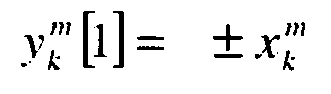
- une étape de calcul des estimées R̂[0] et R̂[1] des matrices de covariance R[0] et R[1] des M vecteurs de mesure ym[0] et ym[1]; cette étape venant se substituer à l'étape de calcul de l'estimée R̂ de la matrice de covariance R des M vecteurs de mesure xm;
- une opération de choix préalable à l'exécution de la boucle de niveau 1 de la quatrième étape ayant pour objet d'effectuer, pour la cellule d'analyse élémentaire (l0, j0) considérée, le test de la parité du paramètre l0 et de déterminer lequel des vecteurs ym[0] et ym[1] et laquelle des estimées R̂[0] et R̂[1] de la matrice de covariance doivent être utilisés pour exécuter la boucle de niveau 1 pour la cellule considérée; la boucle de niveau 1 étant exécutée en utilisant ym[0] et R̂[0] si I0 est pair et en utilisant ym[1]et R̂[1] si l0 est impair.
- a complementary step executed between the step of shaping the received signal samples in the form of M measurement vectors x m , and the step of calculating the matrix of the estimate R of the covariance matrix R; this step carrying out the construction of two sets of measurement vectors y m [0] and y m [1], defined by the following relations:
and - a step of calculating the estimates R [0] and R [1] of the covariance matrices R [0] and R [1] of the M measurement vectors y m [0] and y m [1]; this step being a substitute for the step of calculating the estimate R of the covariance matrix R of the M measurement vectors x m ;
- an operation of choice prior to the execution of the
level 1 loop of the fourth step, the object of which is to carry out, for the elementary analysis cell (1 0 , j 0 ) considered, the parity test of theparameter 1 0 and to determine which of the vectors y m [0] and y m [1] and which of the estimates R [0] and R [1] of the covariance matrix must be used to execute thelevel 1 loop for the considered cell ; thelevel 1 loop being executed using y m [0] and R [0] if I 0 is even and using y m [1] and R [1] if l 0 is odd.
Les caractéristiques et avantages de l'invention seront mieux appréciés grâce à la description qui suit, description qui s'appuie sur les figures annexées qui représentent:
- les
figures 1 à 3 , des chronogrammes illustrant le type de formes d'onde mises en oeuvre préférentiellement par le procédé selon l'invention; - la
figure 4 , une représentation graphique de la pondération en triangle résultant de l'application d'un filtre adapté à une impulsion non modulée reçu par le système mettant oeuvre le procédé selon l'invention; - la
figure 5 , une représentation graphique du module de la fonction de pondération G(Δτ,Δϕ) dans un plan défini par deux axes Distance - Doppler, cette fonction étant à la base du principe d'échantillonnage d'une porte distance considéré par le procédé selon l'invention; - la
figure 6 , une illustration de la grille d'analyse mise en oeuvre par le procédé selon l'invention pour effectuer l'analyse haute résolution d'une porte distance naturelle; - la
figure 7 , l'organigramme du traitement mis en oeuvre par le procédé selon l'invention selon une première forme de réalisation; - la
figure 8 , l'organigramme du traitement mis en oeuvre par le procédé selon l'invention selon une deuxième forme de réalisation; - la
figure 9 , un chronogramme illustrant l'agencement des différentes portes distance dans une forme préférée de mise en oeuvre du procédé selon l'invention; - la
figure 10 , l'organigramme du traitement mis en oeuvre par le procédé selon l'invention selon une troisième forme de réalisation.
- the
Figures 1 to 3 timing diagrams illustrating the type of waveforms implemented preferentially by the method according to the invention; - the
figure 4 , a graphical representation of the triangle weighting resulting from the application of a filter adapted to an unmodulated pulse received by the system implementing the method according to the invention; - the
figure 5 , a graphical representation of the modulus of the weighting function G (Δτ, Δφ) in a plane defined by two Distance-Doppler axes, this function being the basis of the sampling principle of a distance gate considered by the method according to the 'invention; - the
figure 6 an illustration of the analysis grid implemented by the method according to the invention for performing the high-resolution analysis of a natural distance gate; - the
figure 7 the flowchart of the processing implemented by the method according to the invention according to a first embodiment; - the
figure 8 the flowchart of the processing implemented by the method according to the invention according to a second embodiment; - the
figure 9 a timing diagram illustrating the arrangement of the different distance gates in a preferred embodiment of the method according to the invention; - the
figure 10 , the flowchart of the processing implemented by the method according to the invention according to a third embodiment.
Le procédé selon l'invention repose dans un premier temps sur la mise en oeuvre, l'émission, d'une forme d'onde particulière.The method according to the invention is based initially on the implementation, the emission, of a particular waveform.
L'onde émise est ici une séquence de N impulsions 11 non modulées, régulièrement espacées dans le temps d'une période T, comme schématisé sur la
Selon l'invention les récurrences constituant la forme d'onde sont groupées en M paquets appelés "motifs", comme schématisé à la
Chaque motif 21, de rang m, comporte K récurrences, chaque récurrence du motif étant repérée par un indice k à l'intérieur du motif. De la sorte, la forme d'onde est constituée de N = M·K récurrences. Par suite, l'indice courant n d'une récurrence dans la forme d'onde s'écrit n = m·K + k avec 0 ≤ k < K, m représentant l'indice du motif auquel la récurrence est attachée. La fréquence fn de l'onde émise pour cette impulsion n est, quant à elle, notée ![]()
![]()
Selon l'invention, les fréquences ![]()
![]()
![]()
![]()
![]()
![]()
Selon l'invention également, l'application Pm(k) est considérée sous la forme suivante: ![]()
![]()
P(k) et µm représentent des nombres entiers aléatoires, tous les nombres entiers aléatoires P(0),P(1),···,P(K-1),µm étant équi-répartis dans le domaine [0,N[.P (k) and μ m represent random integers, all the random integers P (0), P (1), ···, P (K-1), μ m being equi-distributed in the domain [0 ,NOT[.
Exprimé sous cette dernière forme, un motif m quelconque apparaît donc, selon l'invention, comme la réplique d'un motif générique donné, défini par l'application P(k), translaté en fréquence d'une quantité µm ·Δf, propre à chaque motif m, et recyclé dans le domaine [0,(N-1)·Δf] qui couvre la bande spectrale dédiée à la forme d'onde.Expressed in the latter form, any pattern m therefore appears, according to the invention, as the replica of a given generic pattern, defined by the application P (k), translated in frequency by an amount μ m · Δf, specific to each pattern m, and recycled in the domain [0, (N-1) · Δf] which covers the spectral band dedicated to the waveform.
Selon l'invention, le motif générique décrit par P(k) contient préférentiellement peu de récurrences (typiquement K<10). On parle pour cette raison de "micro-motif" ou encore de "µ-motif".According to the invention, the generic motif described by P (k) preferably contains few recurrences (typically K <10). We speak for this reason of "micro-pattern" or "μ-pattern".
Le type de forme d'onde obtenu par la mise en oeuvre de ce procédé d'attribution des fréquences aux diverses récurrences est illustré par l'exemple de la
Il est à noter que quoique possédant apparemment un certain caractère déterministe, ce principe de détermination de la fréquence associée à une récurrence donnée assure avantageusement le maintien du caractère pseudo-aléatoire du train des impulsions émises sur la durée d'observation, caractère indispensable à une certaine robustesse vis-à-vis des contre-mesures.It should be noted that although having a certain deterministic character, this principle of determining the frequency associated with a given recurrence advantageously ensures the maintenance of the pseudo-random character of the train of the pulses transmitted over the duration of observation, which is essential for a given frequency. certain robustness vis-à-vis the countermeasures.
La forme d'onde mise en oeuvre par le procédé selon l'invention, permet avantageusement de rayonner un signal e(t) qui peut être décrit par la relation suivante: 

Le signal e(t) rayonné est ensuite réfléchi par l'ensemble des P réflecteurs constituant les cibles et l'environnement. Chaque réflecteur p réfléchit, de manière connue, une réplique rp(t) du signal e(t) émis, cette réplique correspondant au signal e(t) affecté d'un retard τp et d'un coefficient complexe ap.The radiated signal e (t) is then reflected by all the P reflectors constituting the targets and the environment. Each reflector p reflects, in known manner, a replica r p (t) of the transmitted signal e (t), this replica corresponding to the signal e (t) affected by a delay τ p and a complex coefficient a p .
Par suite, les signaux réfléchis recueillis par le récepteur formant un signal global reçu r(t), ce signal r(t) s'écrit comme la superposition additive des contributions rp(t) des P réflecteurs éclairés par le signal e(t): 
Les réflecteurs étant généralement des objets mobiles animés d'un mouvement relatif par rapport au radar, le retard τp est une fonction du temps. Cependant, pour les durées de traitement usuellement envisagées, considérées comme très courtes comparativement aux constantes de temps des mouvements relatifs radar/réflecteurs. On considère généralement que la fonction d'évolution du retard τp est une loi linéaire de la forme: ![]()
![]()
ϕp représente ici le Doppler du réflecteur (l.e. le décalage en fréquence dû à l'effet Doppler occasionné par le mouvement du réflecteur) pour la fréquence f0.φ p here represents the Doppler of the reflector (the frequency shift due to the Doppler effect caused by the movement of the reflector) for the frequency f 0 .
On rappelle pour mémoire que la notion de retard (retard de propagation) est équivalente à celle de distance, les deux quantités étant liées par la relation τ=2·D/c où c est la vitesse de la lumière et où le facteur "2" rend compte du trajet aller-retour de l'onde.As a reminder, the notion of delay (propagation delay) is equivalent to that of distance, the two quantities being linked by the relation τ = 2 · D / c where c is the speed of light and where the factor "2 "reports the round trip of the wave.
On rappelle également que la notion de Doppler est équivalente à la notion de vitesse radiale, les deux grandeurs étant liées par la relation ϕ = 2·V / λ où λ est la longueur d'onde.It is also recalled that the notion of Doppler is equivalent to the notion of radial velocity, the two quantities being linked by the relation φ = 2 · V / λ where λ is the wavelength.
De manière générale, avant d'être soumis à un traitement, le signal r(t) reçu passe dans la chaîne de réception qui effectue, récurrence par récurrence, un certain nombre d'opérations de mise en forme, parmi lesquelles on trouve de manière connue:
- la démodulation de la porteuse

- la suppression du Doppler moyen ϕ affectant le signal reçu, ce Doppler moyen étant par exemple défini, à partir de la vitesse
V du porteur et de la direction moyenneu des réflecteurs, par la relation suivante:
- un opération de filtrage ayant pour objet la formation des portes distance dites naturelles. Dans la forme d'implémentation la plus simple, l'application d'un filtre adapté à une impulsion non modulée introduit une pondération en triangle des portes distance naturelles
formées 41, comme cela est schématisé sur lafigure 4 . Cette pondération assimile la largeur de la porte (exprimée en fonction du retard Δτ) à la longueur du segment centré [-Ti, Ti] où Ti est la durée de l'impulsion. - Une opération d'échantillonnage en sortie de filtre.
- demodulation of the carrier
- the suppression of the average Doppler φ affecting the received signal, this average Doppler being for example defined, from the speed
V the wearer and the middle managementu reflectors, by the following relation: - a filtering operation for the purpose of forming the so-called natural distance gates. In the simplest form of implementation, the application of a filter adapted to an unmodulated pulse introduces a triangle weighting of the natural distance gates formed 41, as shown schematically in FIG.
figure 4 . This weighting assimilates the width of the gate (expressed as a function of the delay Δτ) to the length of the centric segment [-T i , T i] where T i is the duration of the pulse. - A sampling operation at the filter output.
En sortie de la chaîne d'opérations décrites précédemment, on dispose ainsi pour chaque porte distance naturelle, définies par la largeur de la réponse du filtre adapté appliqué, d'un signal dit numérisé, constitué d'échantillons (nombres complexes) pouvant faire l'objet d'un traitement numérique implémenté dans un calculateur.At the output of the chain of operations described above, for each natural distance gate, defined by the width of the response of the applied filter applied, a so-called digitized signal consisting of samples (complex numbers) that can be used is thus available. object of a digital processing implemented in a calculator.
. Par suite, moyennant quelques manipulations mathématiques et l'hypothèse non contraignante que ![]()

![]()
![]()
![]()
ap, Δτp et Δϕp représentent respectivement l'amplitude complexe, le retard et le Doppler différentiels relativement à la porte distance traitée pour le premier et au Doppler moyen de la démodulation pour le second.a p , Δτ p and Δφ p respectively represent the differential amplitude, the delay and the Doppler differential with respect to the distance gate processed for the first and the mean Doppler of the demodulation for the second.
Le bruit thermique discrétisé ![]()
![]()
Ainsi, comme on peut le constater en considérant la relation [8] précédente, la sélection par l'invention d'une forme d'onde présentant une agilité de fréquence matérialisée par la fonction Pm(k) permet avantageusement d'obtenir un signal réfléchi échantillonné dont les échantillons ont, sous forme polaire, une expression dans laquelle le terme de phase se présente sous la forme de deux termes additifs séparés, un terme relatif aux retards et un terme relatif aux Dopplers. Une telle séparation des contributions des retards et des Dopplers dans l'expression de la phase d'un échantillon de signal reçu n'est notamment pas possible si l'on définit une forme d'onde comme une fonction linéaire en m et en k.Thus, as can be seen by considering the preceding relation [8], the selection by the invention of a waveform having frequency agility materialized by the function P m (k) advantageously makes it possible to obtain a signal sampled reflection whose samples have, in polar form, an expression in which the phase term is in the form of two separate additive terms, a delay term and a Doppler term. Such a separation of the contributions of the delays and the Dopplers in the expression of the phase of a received signal sample is notably not possible if a waveform is defined as a linear function in m and in k.
Le procédé selon l'invention repose dans un second temps sur la mise en oeuvre d'un traitement particulier, appliqué aux échantillons du signal reçu, traitement rendu possible par l'utilisation de la forme d'onde décrite précédemment. Le traitement selon l'invention, est appliqué aux échantillons d'une porte distance naturelle pour réaliser la discrimination des différents points brillants qu'elle contient. Ce traitement est évidemment destiné à être implémenté pour toutes les portes distance à considérer en l'espèce.The method according to the invention is based in a second step on the implementation of a particular treatment, applied to the samples of the signal received, processing made possible by the use of the waveform described above. The treatment according to the invention is applied to the samples of a natural distance gate to discriminate the different bright spots it contains. This treatment is obviously intended to be implemented for all distance gates to consider in this case.
Selon l'invention les échantillons de signal reçus pour chacune des portes distance sont traités de façon systématique au travers d'une grille d'analyse qui définit la résolution en distance et en Doppler de l'analyse réalisée. Autrement dit les valeurs des paramètres Δτp et Δϕp qui définissent un échantillon ![]()
![]()

![]()
![]()
Chaque échantillon de signal ![]()
![]()
Par suite, pour déterminer la position précise d'un réflecteur, le procédé selon l'invention met en oeuvre un traitement permettant de déterminer les valeurs de coefficients ![]()
![]()
![]()
Therefore, to determine the precise position of a reflector, the method according to the invention implements a process for determining the values of coefficients. ![]()
Selon l'invention, la détermination des coefficients ![]()
![]()
![]()
![]()
![]()
![]()
![]()
![]()
![]()
![]()
![]()
![]()
Par suite chaque coefficient ![]()


![]()
La fonction G(Δτp-1·δτ,Δϕp-j·δϕ) représente la pondération de la contribution du réflecteur p dans le signal reçu dans la porte distance considérée, matérialisée par l'amplitude ap, vis-à-vis de l'amplitude du signal reçu dans la cellule élémentaire (1, j) considérée, amplitude représentée par le coefficient ![]()
![]()
Le module de la fonction de pondération G(Δτ,Δϕ) peut être représenté, comme l'illustre la
Par suite, pour un réflecteur p ayant une position par rapport au détecteur caractérisée par un retard temporel Δτp, un décalage Doppler Δϕp, et une amplitude ap pour la porte distance considérée, une amplitude ![]()

si cette cellule existe, c'est-à-dire si Δτp et Δϕp sont proportionnels respectivement à δτ et δϕ.As a result, for a reflector p having a position relative to the detector characterized by a time delay Δτ p , a Doppler shift Δφ p , and an amplitude a p for the gate distance considered, an amplitude ![]()
if this cell exists, that is, if Δτ p and Δφ p are proportional to δτ and δφ, respectively.
Inversement, 1 et j étant nécessairement des entiers relatifs, si la condition de proportionnalité précédente n'est pas vérifiée le signal présentera pour la cellule (l0, j0) considérée une amplitude atténuée par rapport à cette amplitude maximale.Conversely, since 1 and j are necessarily relative integers, if the preceding proportionality condition is not satisfied, the signal will exhibit for the cell (10 0 , j 0 ) an attenuated amplitude with respect to this maximum amplitude.
Selon l'invention, le pas de quantification (δτ,δϕ), autrement dit le pas de la grille Distance - Doppler ou plus précisément la taille de la cellule élémentaire, est dimensionné de façon à préserver au mieux l'information contenue dans le signal. En pratique, les pas de quantification δτ et δϕ selon l'axe Distance et selon l'axe Doppler sont définis comme suit: 
où N est le nombre de valeurs que peut prendre la fonction Pm(k), et où M·K est le nombre de valeurs que peut prendre m·K+k.According to the invention, the quantization step (δτ, δφ), in other words the pitch of the Distance-Doppler gate or more precisely the size of the elementary cell, is dimensioned so as to best preserve the information contained in the signal . In practice, the quantization steps δτ and δφ along the Distance axis and along the Doppler axis are defined as follows:
where N is the number of values that the function P m (k) can take, and where M · K is the number of values that m · K + k can take.
Ce choix pour les valeurs δτ et δϕ permet avantageusement de dimensionner la cellule élémentaire de telle sorte que la taille de cette cellule élémentaire coïncide avec la largeur du pic de la fonction G pour une amplitude de ce pic correspondant à une atténuation donnée par rapport à son amplitude max. On choisira, par exemple, une cellule dimensionnée pour coïncider avec la largeur du pic à -4dB. La grille représentée sur la
Ainsi, dans le cas le plus défavorable où un réflecteur a une réponse localisée à la limite de la cellule élémentaire (correspondant à un décalage maximum du pic dans la cellule élémentaire), sa contribution dans le signal est mesurée au centre de la cellule élémentaire avec une atténuation donnée par l'amplitude maximale du pic moins 4dB.Thus, in the worst case where a reflector has a localized response at the boundary of the elementary cell (corresponding to an offset maximum of the peak in the elementary cell), its contribution in the signal is measured at the center of the elementary cell with an attenuation given by the maximum amplitude of the peak minus 4 dB.
Par suite les incréments δτ et δϕ étant ainsi définis, le signal ![]()

![]()
La relation [16] montre que la représentation est N-périodique sur l'axe Distance 1 et M·K-périodique sur l'axe Doppler j. Par suite, le domaine de variation des indices 1 et j est défini comme un intervalle limité, une "bande de base" définie par:
- l ∈ [0,N[ pour l'axe Distance,
- j ∈ [0, M.K[ pour l'axe Doppler.
- l ∈ [0, N [for the Distance axis,
- j ∈ [0, MK [for the Doppler axis.
Lors de l'analyse d'une porte distance naturelle donnée par le procédé selon l'invention, la grille ainsi définie est centrée sur la porte distance naturelle analysée, comme illustré à la
Comme on peut le constater, la porte distance naturelle présentant une taille correspondant à 2·Ti, la carte doit couvrir au plus la largeur correspondante 2 · Ti sur l'axe distance. Cette limitation permet avantageusement de déterminer un majorant du nombre N de fréquences considérées. On a ainsi: ![]()
![]()
Par ailleurs, l'analyse de la séquence temporelle des échantillons du signal permet de développer l'axe Doppler à l'intérieur de la porte distance. Le nombre total M·K des récurrences traitées doit être aussi grand que possible pour accroître la résolution. Cependant, des considérations opérationnelles imposent des valeurs limites à ce nombre de récurrences. Par suite, le traitement mis en oeuvre par le procédé selon l'invention recherche, pour chaque porte distance naturelle, les valeurs des N·M·K coefficients ![]()
![]()
![]()
![]()
Il est à noter que la connaissance des M·K échantillons ![]()
![]()
![]()
![]()
C'est pourquoi le traitement selon l'invention met à profit le fait que par hypothèse, les points brillants étant en nombre limité, il est certain qu'un très grand nombre de coefficients ![]()
![]()
![]()
![]()
La
La première étape 71 du traitement consiste à acquérir pour le cycle de N récurrences considéré, les termes P(k) et µm définissant les µ-motifs utilisés à l'émission pour générer la forme d'onde. Ces termes, déterminés à l'émission, sont ensuite mémorisés pour pouvoir être utilisés par le traitement.The
La deuxième étape 72 du traitement mis en oeuvre par le procédé selon l'invention consiste quant à elle dans le conditionnement des K·M échantillons ![]()

"T" représentant l'opérateur de transposition.The ![]()
"T" representing the transposition operator.
Par suite chaque vecteur de mesure xm peut avantageusement être représenté par la relation suivante: 
![]()
![]()
En outre, en considérant une cellule élémentaire particulière repérée par ses coordonnées (l0,j0) sur la grille d'analyse (i.e. la carte), un vecteur xm peut avantageusement être mis sous la forme suivante: 
xm est ainsi représenté pour la cellule élémentaire considérée comme la somme d'un signal utile ![]()

![]()
Il est à noter ici que, le signal Vm correspondant à la somme du signal parasite ![]()
![]()
La matrice de covariance Q, non accessible en tant que telle du fait du nombre d'inconnues, peut cependant avantageusement être estimée, de manière connue, à partir d'une moyenne temporelle, pour peu que les signaux vectoriels xm aient une covariance indépendante de m.The covariance matrix Q, which is not accessible as such because of the number of unknowns, can however advantageously be estimated, in a known manner, from a time average, provided that the vector signals x m have an independent covariance. from m.
Dans le cadre du procédé selon l'invention cette condition de "stationnarité" est avantageusement remplie. En effet, celui-ci met en oeuvre des formes d'ondes remplissant la condition générale définie pour tout motif m, par la relation suivante: ![]()
![]()
La condition [21] est en particulier vérifiée pour des formes d'onde vérifiant la relation suivante: ![]()
![]()
Pour de telles formes d'ondes, la connaissance de tous les termes µm (µm = Pm (0)) pour m ∈ [0,M[, et de tous les termes P(k) (P(k)= S(k,0) dans la relation [21]) définis indépendamment de m pour k ∈ [0,K[, permet avantageusement de définir la séquence complète des fréquences, Pm(k), mises en oeuvre pour les K récurrences d'un motif m.For such waveforms, the knowledge of all the terms μ m (μ m = P m (0)) for m ∈ [0, M [, and of all the terms P (k) (P (k) = S (k, 0) in the relation [21]) defined independently of m for k ∈ [0, K [, allows advantageously to define the complete sequence of frequencies, P m (k), implemented for K recurrences of a pattern m.
La relation [21] définit ainsi les formes d'onde mise en oeuvre par le procédé selon l'invention. La relation [22] définit quant à elle les formes d'onde préférées de l'invention. Plus précisément, dans une forme préférée de réalisation, le procédé selon l'invention met en oeuvre, comme cela a été dit précédemment, des formes d'ondes pour lesquelles tous les nombres P(0),P(1),...,P(K-1),µm sont des nombres entiers aléatoires, équi-répartis dans le domaine [0,N[, P(k) représentant un motif générique, ou micro motif.The relationship [21] thus defines the waveforms implemented by the method according to the invention. The relationship [22] defines the preferred waveforms of the invention. More specifically, in a preferred embodiment, the method according to the invention implements, as has been said previously, waveforms for which all the numbers P (0), P (1), ... , P (K-1), μ m are random integers equi-distributed in the domain [0, N [, P (k) representing a generic pattern, or micro-pattern.
Selon cette forme de réalisation préférée, les formes d'ondes préférées sont, par ailleurs, plus précisément définies, de manière à restreindre le domaine de variation des Pm(k) au segment [0,N[ et donc de restreindre le nombre des fréquences disponibles à l'émission à N, par la relation [4] qu'on rappelle ici: ![]()
![]()
Par suite, avec cette famille de formes d'onde, les vecteurs gm(l,j) peuvent avantageusement être définis par la relation suivante: ![]()
![]()
![]()
![]()
![]()
![]()
Par suite, un vecteur de mesure xm a pour expression: ![]()
![]()
Il est à noter que, puisque le signal contient le bruit thermique (bruit blanc), aucune valeur propre de Q n'est nulle et donc la matrice est inversible.It should be noted that, since the signal contains thermal noise (white noise), no eigenvalue of Q is zero and therefore the matrix is invertible.
La troisième étape 73 du traitement mis en oeuvre par le procédé selon l'invention consiste à réaliser une estimation Q̂ de la matrice de covariance Q, estimation réalisée au travers de l'estimation R̂ de la matrice de covariance R des M vecteurs de mesure xm.The
Il est en effet à noter que l'objet du traitement appliqué étant de caractériser la présence éventuelle d'un réflecteur dans une cellule d'analyse élémentaire donnée, seule la connaissance des coefficients ![]()
![]()
![]()
![]()
Selon l'invention, vm étant considéré comme gaussien, la fonction de densité de probabilité conjointe des mesures peut être explicitée pour réaliser une estimation optimale au sens du maximum de vraisemblance du coefficient ![]()
![]()
En pratique, on tire de cette fonction de densité de probabilité conjointe l'estimée ![]()
![]()

![]()
![]()
Le terme z(l0,,j0) représente ici une intégration cohérente des mesures sur les µ-motifs, définie par la relation suivante: 
L'expression de l'estimation ![]()
![]()
![]()
![]()
Selon ce mode d'estimation, non basé sur la probabilité conjointe, l'estimée Q̂ est définie par la relation: 

Par suite, l'inverse de la matrice Q̂, estimée de Q, peut être explicitée, de sorte que l'on dispose d'un système des deux équations à deux inconnues définissant les estimées, ce système étant décrit par les relations suivantes: 
L'élimination de Q̂-1 entre ces deux équations fournit l'estimation recherchée de ![]()
![]()
Ainsi, l'objet de la troisième étape 73 du traitement mis en oeuvre par le procédé selon l'invention consiste principalement à réaliser le calcul de la matrice de covariance estimée R̂ des M vecteurs xm, matrice de dimension K·K.Thus, the object of the
Cependant, bien qu'en raison de la présence du bruit thermique, la matrice de covariance R n'ait aucune valeur propre nulle et qu'elle soit donc théoriquement inversible, son estimée R̂ peut s'avérer numériquement très proche de la singularité. Dans un tel cas le calcul de l'expression du module ρ̂2(l0,j0) serait pris en défaut. C'est pourquoi, pour se prémunir contre cette éventualité, le traitement mis en oeuvre au cours de l'étape 73 peut également comporter, dans une forme préférée, une opération de "chargement de la diagonale" de la matrice, consistant à ajouter aux éléments diagonaux de la matrice R̂ des quantités (aléatoires) réelles positives (puisque la matrice est hermitienne) petites devant la plus grande valeur propre.However, although due to the presence of thermal noise, the covariance matrix R has no zero eigenvalue and is therefore theoretically invertible, its estimate R can be numerically very close to the singularity. In such a case, the calculation of the expression of the module ρ 2 (l 0 , j 0 ) would be faulted. Therefore, to guard against this eventuality, the processing implemented during
La quatrième étape 74 du traitement mis en oeuvre par le procédé selon l'invention consiste à utiliser la matrice de covariance empirique R̂ des mesures, calculée à l'étape précédente, pour résoudre, pour chaque cellule d'analyse (l,j), le système [29] et réaliser l'opération proprement dite de caractérisation de la présence d'un réflecteur.The
Dans un premier mode de réalisation du procédé selon l'invention, l'opération réalisée par le traitement consiste à calculer, pour chaque cellule (l,j), le module ![]()
![]()

![]()
![]()
Le terme ρ̂2(l0,j0) ainsi calculé représente une estimation de l'énergie reçue provenant d'un réflecteur localisé dans la cellule élémentaire considérée (l 0,j 0).The term ρ 2 (1 0 , j 0 ) thus calculated represents an estimate of the energy received from a reflector located in the elementary cell in question ( l 0 , j 0 ).
Un balayage suivant les indices 1 et j permet de générer la carte complète associée à la porte distance naturelle dans laquelle a été prélevé le signal.A scan according to
Dans cette première forme de réalisation, le traitement selon l'invention permet ainsi de disposer pour chaque cellule d'analyse (l,j) du niveau de signal reçu et de former ainsi pour chaque porte distance naturelle, une table des estimations du niveau de signal reçu. Ces estimations peuvent ainsi être transmises sous cette forme à un traitement ultérieur pouvant les exploiter de manière diverse.In this first embodiment, the processing according to the invention thus makes it possible to have for each analysis cell (l, j) the received signal level and thus form for each gate natural distance, a table of the estimates of the level of the received signal. These estimates can thus be transmitted in this form to a subsequent processing that can exploit them in various ways.
D'un point de vue pratique, la quatrième étape 74 du traitement mis en oeuvre par le procédé selon l'invention considère et traite les cellules d'analyse élémentaires l'une après l'autre.From a practical point of view, the
A cet effet elle exécute, pour l'ensemble des µ-motifs, une opération itérative 741 consistant, à chaque itération à considérer un µ-motif particulier, et à prendre en compte (à "charger") le vecteur de mesure xm et à réaliser pour la cellule d'analyse élémentaire (l,j) considérée, le calcul incrémental permettant de déterminer le vecteur z(l,j) correspondant à l'intégration cohérente des vecteurs de mesures xm sur l'ensemble des µ-motifs, ce calcul étant défini par la relation suivante: 
Chaque itération est terminée par un test permettant de déterminer si l'ensemble des M µ-motifs a été pris en compte et de relancer une itération si tel n'est pas le cas.Each iteration is completed by a test to determine if the set of M μ-patterns has been taken into account and to restart an iteration if this is not the case.
Ainsi, à l'issue des M itérations correspondant à l'exploitation des M vecteurs de mesures xm l'opération 741 délivre la valeur finale du vecteur z(l,j) pour la cellule d'analyse élémentaire (l,j) considérée.Thus, at the end of the M iterations corresponding to the exploitation of the M measurement vectors x m, the
Selon l'invention l'exécution des M itérations de l'opération 741 est précédée par l'exécution d'une opération 743 d'initialisation consistant à mettre à 0 le vecteur des mesures z et à calculer le vecteur b(l,j) des termes de phase correspondant à la cellule d'analyse considérée.According to the invention, the execution of the M iterations of the
Elle est par ailleurs suivie par l'exécution d'une opération 742 de calcul de la valeur du module ρ̂2(l,j) correspondant à la cellule élémentaire (l,j) considérée.It is furthermore followed by the execution of an
Selon l'invention les opérations 742 et 743, ainsi que les M itérations d'exécution de l'opération 741 sont répétées pour chacune des cellules d'analyses élémentaires (l,j), en considérant toutes les valeurs possibles de Doppler et, pour chaque valeur de Doppler, toutes les valeurs possibles de distance, compte tenu du pas de la grille d'analyse. Autrement dit on considère, toutes les valeurs du paramètre j et, pour chaque valeur de j, toutes les valeurs du paramètre 1.According to the invention the
Par suite, comme l'illustre la
La boucle de premier niveau 75 met en oeuvre M fois l'opération 741.The
La boucle de second niveau 76 exécute quant à elle, pour chacune des cellules d'analyse correspondant à une même valeur du Doppler, l'opération d'initialisation 743. Elle lance ensuite l'exécution de la boucle de premier niveau 75, puis l'exécution de l'opération 742 de calcul de ρ̂2(l,j).The second-
La boucle de troisième niveau 77, enfin, gère l'ensemble des valeurs de Doppler possibles et lance l'exécution de la boucle de deuxième niveau 76 pour chaque valeur du Doppler.The
On obtient ainsi comme l'illustre la
Ainsi dans son premier mode de réalisation, le procédé selon l'invention permet avantageusement d'obtenir pour chaque porte distance naturelle prise séparément, une estimation fine en distance et en Doppler du niveau (i.e. de la puissance) de signal reçu en provenance d'un réflecteur localisé dans la cellule d'analyse élémentaire (l,j) considérée, cette estimation étant débarrassée de la contribution des signaux parasites. Cependant, II existe beaucoup d'applications qui ne nécessitent pas de connaitre l'estimation de l'énergie reçue dans chaque cellule élémentaire. L'information recherchée, de nature binaire, peut parfois se réduire dans certains cas à déterminer s'il y a ou non présence d'un point brillant, dans la cellule d'analyse considérée, c'est-à-dire d'un réflecteur localisé à la distance considéré et présentant un Doppler donné.Thus, in its first embodiment, the method according to the invention advantageously makes it possible to obtain for each natural distance gate taken separately, a fine estimate in distance and in Doppler of the level (ie of the power) of signal received from a reflector located in the elementary analysis cell (l, j) considered, this estimate being rid of the contribution of parasitic signals. However, there are many applications that do not require knowing the estimate of the energy received in each elementary cell. The information sought, of a binary nature, can sometimes be reduced in certain cases to determine whether or not there is a bright spot, in the analysis cell under consideration, that is to say, a reflector located at the distance considered and having a given Doppler.
Par suite dans une deuxième mode de réalisation, le traitement implémenté par le procédé selon l'invention consiste alors à permettre de catégoriser la cellule considérée en considérant que le signal reçu peut être modélisé par deux formes distinctes possibles suivant les hypothèses H1 et H0 de présence ou non d'un point brillant (i.e. d'un réflecteur):
- Hypothèse H0: absence de point brillant (I.e. absence de réflecteur). xm correspond alors seulement à un signal parasite:

- Hypothèse H1: présence d'un point brillant (I.e. présence d'un réflecteur). xm correspondant alors à un signal utile associé à une signal parasite:
- Hypothesis H 0 : absence of bright spot (no reflector). x m then corresponds only to a spurious signal:
- Hypothesis H 1 : presence of a bright spot (the presence of a reflector). x m then corresponding to a useful signal associated with a parasitic signal:
Le traitement réalisé par le procédé selon l'invention a alors pour objet de déterminer, à partir des mesures disponibles, laquelle des hypothèses H1 ou H0 est la bonne.The treatment carried out by the method according to the invention is then intended to determine, from the available measurements, which of the hypotheses H 1 or H 0 is the right one.
Selon l'invention, la détermination est réalisée en considérant le critère de NEYMAN-PEARSON. Ce critère est jugé optimal au sens où il assure une probabilité de détection maximale tout en maintenant le taux de fausse alarme inférieur à une valeur donnée. Il conduit à un test basé sur le rapport de vraisemblance, de la forme: 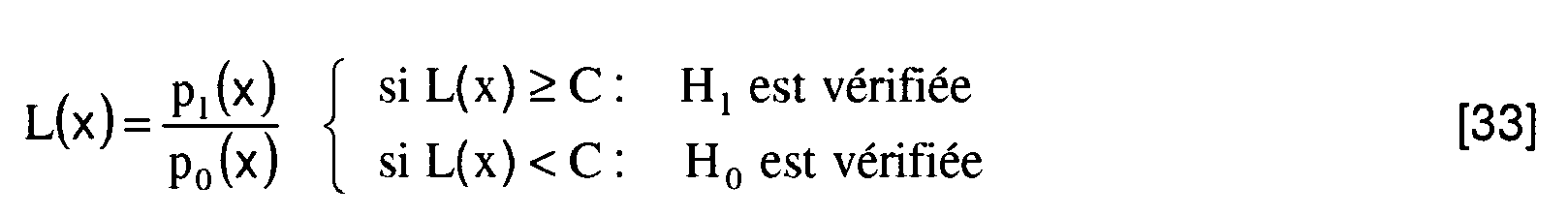
C représente ici un seuil qui s'exprime en fonction de la probabilité de fausse alarme fixée, et qu'il faut déterminer.According to the invention, the determination is made by considering the NEYMAN-PEARSON criterion. This criterion is considered optimal in the sense that it ensures a maximum probability of detection while keeping the false alarm rate lower than a given value. It leads to a test based on the likelihood ratio, of the form:
C represents here a threshold which is expressed as a function of the probability of fixed false alarm, and which must be determined.
Dans le contexte de l'invention et après développement des calculs en reprenant les notations utilisées précédemment, le test considéré, qui a la qualité d'être "uniformément plus puissant", peut être formulé de la façon suivante: 
Le calcul de C s'appuie quant à lui sur la définition de la probabilité de fausse alarme, notée Pfa, qui est la probabilité d'être supérieur à C sous l'hypothèse H0 : 
Par suite, sachant que sous l'hypothèse H0 les mesures son modélisées par xm = v m et connaissant la nature statistique gaussienne des vecteurs v m , cette probabilité Pfa peut être explicitée pour en déduire l'inconnue C : 
Le test effectué prend alors la forme suivante: 

Le test théorique [37] peut alors être remplacé par le test opérationnel défini par: 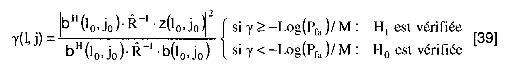
Ainsi, dans ce second mode de réalisation du procédé selon l'invention, l'étape 74 du traitement consiste à mettre en oeuvre non plus l'opération 742 consistant à calculer ρ̂2(l,j), mais une opération 842 consistant à calculer le terme γ(l,j) et à comparer la valeur obtenue pour chaque cellule d'analyse (l,j) à S=-Log(Pfa)/M, comme l'illustre l'organigramme de la
On obtient alors une carte qui se présente sous la forme d'une table 88 définissant chacune des cellules élémentaires de taille (δτ, δϕ) de la porte distance considérée par un critère dont la valeur, 1 ou 0 par exemple, indique seulement la présence d'un réflecteur ou non.A map is then obtained which is in the form of a table 88 defining each of the elementary cells of size (δτ, δφ) of the gate distance considered by a criterion whose value, 1 or 0 for example, only indicates the presence reflector or not.
Il est à noter qu'à cause d'une normalisation différente au dénominateur, la quantité γ(l0,j0) testée par le traitement dans ce second mode de réalisation du procédé selon l'invention, ne correspond pas exactement à l'estimée ρ̂2(l0,j0) du problème précédent. Cependant, la similitude des numérateurs indique que le traitement de décision relève du même procédé de projection que celui utilisé par le traitement d'estimation du premier mode de réalisation.It should be noted that because of a different normalization to the denominator, the quantity γ ( 10 0 ) tested by the treatment in this second embodiment of the method according to the invention does not correspond exactly to the estimated ρ 2 (l 0 , j 0 ) of the previous problem. However, the similarity of the numerators indicates that the decision processing is in the same projection method as used in the estimation process of the first embodiment.
Les deux modes de réalisation du procédé selon l'invention décrits dans le texte qui précède, peuvent avantageusement être combinés, l'opération de détection 842 du traitement implémenté dans le second mode de réalisation pouvant être associé à l'opération d'estimation 742 du traitement implémenté dans le premier mode, de façon à réaliser un nettoyage de fond de carte, dont le principe est de multiplier cellule à cellule la table des niveaux de signal 78 par la table binaire 88 de façon à mettre à 0 les cellules pour lesquelles il n'y a pas eu détection (γ(l,j)<S) et à ne conserver que les estimations des cellules pour lesquelles une détection a été réalisée (γ(l,j)≥S).The two embodiments of the method according to the invention described in the preceding text can advantageously be combined, the
Comme cela a été dit précédemment, le procédé selon l'invention tel que décrit est appliqué à un certain nombre de portes distance naturelles suivant l'étendue de l'objet à observer. Par suite l'espace observé se présente sous la forme d'une juxtaposition de cartes unitaires à haute résolution chaque carte correspondant à une porte distance. Généralement, de façon à limiter le nombre de portes distance à considérer l'espace observé est divisé en cartes juxtaposées. Cependant, cette manière de procéder quoique avantageuse dans le cas d'objets (de réflecteurs) d'étendues restreintes, couverts par une seule porte distance, nécessite, dans le cas d'objets plus étendus, de prendre en compte plusieurs portes distance simultanément, une carte unique ne couvrant qu'une faible partie de l'objet. Assembler judicieusement différentes cartes pour reconstituer l'objet complet offre alors un intérêt opérationnel évident.As has been said previously, the method according to the invention as described is applied to a certain number of natural distance gates according to the extent of the object to be observed. As a result, the space observed is in the form of a juxtaposition of high-resolution unit maps, each map corresponding to a distance gate. Generally, so as to limit the number of gates distance to consider the observed space is divided into juxtaposed cards. However, this way of proceeding though advantageous in the case of objects (reflectors) restricted areas, covered by a single door distance, requires, in the case of larger objects, to take into account several doors simultaneously distance, a single card covering only a small part of the object. Judicially assembling different cards to reconstitute the complete object then offers an obvious operational interest.
Or, compte tenu de la pondération triangulaire induite par le filtrage adapté lors de la formation des portes distance, les points brillants subissent une atténuation d'autant plus forte qu'ils sont plus décentrés dans la porte. C'est pourquoi l'assemblage des cartes ne peut pas être effectué par une simple juxtaposition des cartes produites, sous peine d'introduire une modulation d'amplitude extrêmement préjudiciable à une exploitation ultérieure de la carte composite globale regroupant toutes les portes distance analysées. Par suite, le procédé mis en oeuvre consiste alors non pas à considérer des portes distance juxtaposées mais des portes distance 91 présentant un recouvrement, tel que l'illustre la
Ainsi, en restreignant à sa seule partie centrale 92 la contribution de chaque porte naturelle 91 à la constitution d'une carte globale, ou plus précisément la contribution de chaque carte haute résolution associée, on ne retient en effet que les échos les moins atténués.Thus, by restricting to its only
Selon l'invention, la largeur ΔτC de cette partie centrale 92 est choisie en fonction de l'atténuation α maximale tolérée, suivant la relation: ![]()
![]()
Par suite, le recouvrement est obtenu lors de l'application du filtre adapté, en imposant le pas ΔτC à la formation des portes distance naturelles.As a result, the overlap is obtained during the application of the matched filter, by imposing the pitch Δτ C on the formation of the natural distance gates.
Ainsi, comme l'illustre l'exemple de la
Ainsi grâce à cet agencement particulier des portes distance, l'ensemble des points brillants est avantageusement bien mieux rendu dans la carte composite finale que dans chaque carte unitaire 1, 2, 3 ou 4.Thus, thanks to this particular arrangement of the distance gates, the set of bright points is advantageously better rendered in the final composite card than in each
Il est à noter que ce phénomène de juxtaposition n'a pas d'incidence sur l'axe Doppler, car la bande restituée par la carte est commune à toutes les portes distance naturelles. L'assemblage des cartes (des tables) n'est à opérer que suivant l'axe distance.It should be noted that this juxtaposition phenomenon does not affect the Doppler axis, because the band restored by the card is common to all natural distance gates. The assembly of the cards (tables) is to operate only along the distance axis.
Dans le cas des deux premiers modes de réalisation du procédé selon l'invention décrits précédemment, la taille maximale d'une cellule est donnée par le pas d'échantillonnage (δτ, δϕ) de la grille d'analyse de la porte distance, pas défini de façon à obtenir la résolution souhaitée. Par suite, le pas d'échantillonnage du signal est défini de manière précise.In the case of the first two embodiments of the method according to the invention described above, the maximum size of a cell is given by the sampling step (δτ, δφ) of the distance gate analysis grid, not defined to achieve the desired resolution. As a result, the sampling step of the signal is precisely defined.
En pratique, comme cela a été dit précédemment, les pas de quantification δτ et δϕ selon l'axe Distance et selon l'axe Doppler sont définis comme suit (cf. relation [15]): 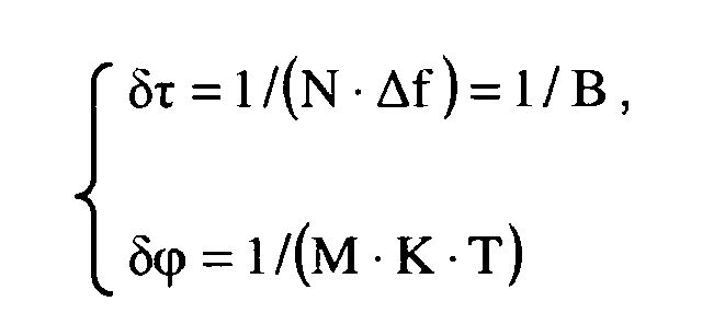
où N est le nombre de valeurs que peut prendre la fonction Pm(k), et où M·K est le nombre total d'impulsions émises.In practice, as has been said previously, the quantization steps δτ and δφ along the Distance axis and along the Doppler axis are defined as follows (see relation [15]):
where N is the number of values that the function P m (k) can take, and where M · K is the total number of pulses emitted.
Cependant, II convient de distinguer les notions de résolution et d'échantillonnage.However, the concepts of resolution and sampling should be distinguished.
On rappelle ici que la résolution correspond au pouvoir séparateur offert par le traitement. Elle est caractérisée par les dimensions du pic de la réponse impulsionnelle à un point brillant (i.e. à l'origine d'un signal de forte puissance), comptées généralement à -4dB du sommet (cf.
Par suite, compte tenu d'une résolution donnée, la question se pose de l'échantillonnage optimal du signal reçu dans une porte distance. Autrement dit, en se figurant l'espace restitué comme une surface ondulée, comme illustré par la
Selon l'invention, l'échantillonnage du signal reçu (de la surface 51) est préférentiellement réalisé de façon à échantillonner celui-ci aux centres de cellules juxtaposées dont la taille est précisément égale à la résolution. Ce choix est motivé d'une part pour le besoin de contrôler l'atténuation de restitution d'un points brillants dont la position ne correspond pas exactement au centre d'une cellule d'analyse, et d'autre part par le besoin de s'affranchir de l'opérateur de congruence modulo N introduit dans le terme de phase relatif au retard par la fonction Pm (k) . Cette fonction s'écrit en effet: 
![]()
![]()
![]()
![]()
Or, 1 et ![]()
![]()

![]()
![]()
Par suite si le pas d'échantillonnage en distance est modifié, en particulier s'il est diminué (suréchantillonnage) le traitement du terme de phase doit subir une modification notable et devient difficile à implémenter. Toutefois, dans un mode de réalisation particulier, le procédé selon l'invention permet d'exécuter un doublement de l'échantillonnage à taille de cellules constante, associé à un chevauchement moitié des cellules d'analyse. Dans un tel mode opératoire, l'indice 1 caractérisant la distance de la cellule considérée dont dépend le terme de phase n'est plus entier. Cependant 1 n'est pas défini de manière quelconque et peut se mettre sous la forme fractionnaire suivante: ![]()
![]()
Par suite, le terme de phase peut être exprimé par la relation suivante: ![]()
![]()
![]()
![]()
Par suite un échantillon de signal reçu est défini par la relation suivante (en notant 1 l'indice distance sur-échantillonnée): 
![]()

![]()
Ainsi, en considérant une cellule d'analyse particulière, la cellule courante (l0,j0), la relation précédente peut encore s'écrire: ![]()
![]()
où le terme ![]()
![]()
Par suite, pour traiter selon l'invention le signal correspondant à ce cas particulier de sur-échantillonnage, il est seulement nécessaire de distinguer deux familles d'échantillons: une pour les valeurs paires de l0 et une pour les valeurs impaires. On définit alors un nouveau signal tabulé à double entrée défini par: 
Cette construction est possible car on dispose de tous les éléments pour calculer η. Son intérêt vient du fait qu'en traitant le signal ![]()
![]()
![]()
soit encore, vectoriellement en introduisant les mesures ![]()

![]()
![]()
![]()
again, vectorially by introducing the measurements ![]()
Par suite, le modèle de vecteur de mesure utilisé a une structure strictement identique au vecteur xm auquel est appliqué le traitement implémenté par le procédé selon l'invention dans les deux modes décrits précédemment. Le traitement décrit précédemment s'applique donc avantageusement à ce cas de suréchantillonnage, moyennant une adaptation permettant de travailler sur un double jeu de vecteurs de mesures ym[0] et ym[1] pour chacun desquels il faut calculer les matrices de covariance R̂[0] et R̂[1] et les inverser. Le traitement ainsi adapté peut être décrit par l'organigramme de la
Comme on peut le constater sur la figure, le traitement mis en oeuvre dans ce mode de réalisation particulier présente, par rapport aux modes de réalisation précédents:
une étape 102 d'acquisition des vecteurs de mesures xm et de constitution des vecteurs ym[0] et ym[1]; cette étape se substituant à l'étape 72 des modes de réalisation desfigures 7 et8 ;une étape 103 de calcul des matrices de covariance estimées R̂[0] et R̂[1] des vecteurs de mesure ym[0] et ym[1]; cette étape se substituant à l'étape 73 des modes de réalisation desfigures 7 et8 .une opération 144 qui prend place dansl'étape 74 dans la boucle de niveau 2 (boucle sur les distances) avant l'exécution de la boucle 76 de niveau 1 (boucle sur les µ-motif) et dont l'objet est de déterminer pour chaque valeur du paramètre 1, si celui-ci est pair ou impair et si on considère ym[0] et R̂[0] ou ym[1] et R̂[1].
- a
step 102 for acquiring vectors of measurements x m and for constituting vectors y m [0] and y m [1]; this step substituting forstep 72 of the embodiments of thefigures 7 and8 ; - a
step 103 for calculating the estimated covariance matrices R [0] and R [1] of the measurement vectors y m [0] and y m [1]; this step substituting forstep 73 of the embodiments of thefigures 7 and8 . - an
operation 144 which takes place in thestep 74 in thelevel 2 loop (loop on the distances) before the execution of theloop 76 of level 1 (loop on the μ-pattern) and whose object is to determine for each value ofparameter 1, if it is odd or even and if it is considered m [0] and R [0] and y m [1] and R [1].
Le reste des étapes de traitement reste par ailleurs inchangé.The rest of the processing steps remain unchanged.
Il est à noter que, comme l'illustre la figure 11, la contrainte de distinction de valeurs paires et impaires du paramètre 1 ne trouve pas d'équivalent en ce qui concerne le paramètre Doppler j, de sorte que la boucle 77 de niveau 3 n'est pas affectée. En effet l'exploration de l'axe Doppler ne met pas en jeu d'opérateur de congruence. Un sur-échantillonnage sur cet axe ne pose donc aucun problème particulier, hormis le volume de calculs accru.It should be noted that, as shown in FIG. 11, the odd and even value distinction constraint of the
Il est à noter en outre que ce mode de réalisation particulier, décrit ici pour un échantillonnage double de chaque porte distance, peut être généralisé de manière analogue à un sur-échantillonnage d'un facteur entier supérieur à 2, au prix toutefois d'une complexification algorithmique importante.It should be further noted that this particular embodiment, described here for double sampling of each gate distance, may be generalized analogously to oversampling of an integer factor. greater than 2, but at the price of significant algorithmic complexity.
Claims (11)
- A method for carrying out a high-resolution range and Doppler analysis of radio signals received from a given area of space, said received signals being analysed by baseband, after applying matched filtering, through so-called range gates, defined by the width of the response of the applied matched filter, characterised in that it comprises:- transmitting a particular waveform comprising M packets of K pulses, referred to as patterns, of duration Ti, transmitted with a recurrence period T, the frequencies of the K pulses being determined in a given assigned frequency band B, the pulse frequencies forming the same pattern m being defined in the band B, for any two returns k and k', by the following relation:

where S(k, k') represents any function of k and k' independent of m, Pm(k) representing the completion of random draws that all differ from the frequencies transmitted for the K recurrences of the pattern m;- receiving the signal originating from the area in the considered space and sampling the signal received for each of the natural range gates, of width 2Ti, the signal being sampled by delay and by Doppler according to a sampling step (δτ, δϕ) defined by the following relation:
where N is the number of values that can be assumed by the function Pm(k), i.e. the number of assigned frequencies, and where M˙K is the total number of transmitted pulses;
the natural range gate thus being divided into elementary analysis cells, each elementary cell being identified by the parameters 1 and j characterising its position by range and by Doppler in the sampling space of the natural range gate;- processing the received signal for a given range gate, said processing comprising:- shaping received signal samples spatially corresponding to the considered range gate in the shape of M measurement vectors xm, each vector having as components the K received signal samples temporally corresponding to the K recurrences of the pattern m;- calculating the estimate R of the covariance matrix R of the M measurement vectors xm;- executing a characterisation operation, which consists in calculating, for each analysis cell (l, j), a magnitude allowing an estimate of the level of the received signal to be carried out in the considered analysis cell and which is likely to originate from a reflector located within the range gate corresponding to the range characterising said cell (1, j), the value of this magnitude being determined on the basis of the coherent integration of the vectors xm over all of the patterns and of the estimated matrix R̂ ;- developing a table comprising, for each analysis cell, the value of the considered magnitude. - The method according to claim 1, characterised in that with Pm(k) being defined by the following relation:
 P(k) and µm representing random integers, all of the random integers, P(0), P(1),...,P(K - 1), µm being equally distributed in the domain [O, N[;
each of the frequencies fk m of the pulses forming a given pattern m is defined, for a pulse k of the pattern, by the following relation:
in which fo is the base carrier frequency of the transmitted pulses and Δf is the quantification step of the transmission frequencies defined by Δf = B / N. - The method according to claim 1 or 2, characterised in that the magnitude characterising the received signal level for a given analysis cell (l0, j0), calculated (742) by the signal processing, is the energy estimate ρ̂2 (l0, j0) defined by the following relation:

in which b(lo, jo) is a vector expressed as:
with

with
- The method according to claim 3, characterised in that the processing implemented for each range gate comprises:- a first processing step (71) that consists in acquiring the terms P(k) and µm defining the patterns used during the transmission;- a second step (72) that consists in conditioning the K·M samples xk m of the received signal in the shape of M measurement vectors xm, each vector having as components the K samples corresponding to the K recurrences of the same pattern m that are defined by the following relation:where xk m represent the received signal sample corresponding to the transmission of the pulse k of the pattern m;
 - a third step (73) that consists in determining the estimate R̂ of the covariance matrix R of the M measurement vectors xm, R̂ being defined by the following relation:
 - a fourth step (74) that considers and processes the elementary analysis cells (l, j) one after the other and determines the value of the magnitude ρ̂2(l, j) for each cell;the execution of the fourth step leading to the development of a table comprising the value of the magnitude ρ̂2(l,j) for each analysis cell.
 - The method according to claim 4, characterised in that the fourth step (74) implements three nested processing loops:- a first level loop (75) that executes, for each of the elementary analysis cells (l, j), an iterative operation (741) that consists in, upon each iteration, considering a particular pattern and in calculating the current value of the vector z(l, j) defined by the following relation:

each iteration being terminated by a test for determining if the set of M patterns has been taken into account and restarting an iteration if this is not the case;- a second level loop (76) which, for each of the analysis cells (l, j) corresponding to the same value of the Doppler parameter j, executes in an iterative manner an operation (743) for setting the vector z to 0 and for constructing the vector b, then launches the execution of the first level loop (75) and the execution of the operation (742) for calculating ρ̂2 (l, j); each iteration being terminated by a test for determining if the set of values of the parameter 1 has been taken into account and restarting an iteration if this is not the case;- a third level loop (77) which manages the set of values of the Doppler parameter j and launches the iterative execution of the second level loop (76) for each value of j; each iteration being terminated by a test for determining if the set of values of the parameter j has been taken into account and restarting an iteration if this is not the case. - The method according to claim 1 or 2, characterised in that the magnitude characterising the received signal level calculated for a given analysis cell (l0, j0), calculated (742) by the signal processing, is a magnitude γ(l0, j0) defined by the following relation:

in which b(lo, jo) is a vector expressed as:
with

with
this magnitude being used to detect reflectors, a detection being identified when the value of γ(l0, j0) is greater than a fixed threshold, said threshold being a function of a given false alarm probability. - The method according to claim 6, characterised in that the processing implemented for each range gate comprises:- a first processing step (71) that consists in acquiring the terms P(k) and µm defining the patterns used during the transmission and which are saved to this end;- a second step (72) that consists in conditioning the K·M samples xk m of the received signal in the form of M measurement vectors xm, each vector having as components the K samples corresponding to the K recurrences of the same pattern m being defined by the following relation:

where xk m represents the received signal sample corresponding to the transmission of the pulse k of the pattern m;- a third step (73) that consists in determining the estimate R̂ of the covariance matrix R of the M measurement vectors xm, R̂ being defined by the following relation: - a fourth step (74) that considers and processes the elementary analysis cells (l, j) one after the other and determines for each cell the value of the magnitude y(l, j) and determines if a reflector is detected in the considered cell;
the execution of the fourth step leading to the development of a table comprising for each analysis cell the value 1 or 0 of the detection criterion. - The method according to claim 7, characterised in that the fourth step (74) implements three nested processing loops:- a first level loop (75) that executes, for each of the elementary analysis cells (l, j), an iterative operation (741) that consists in, upon each iteration, considering a particular pattern and in calculating the current value of the vector z(l, j) defined by the following relation:

each iteration being terminated by a test for determining if the set of M patterns has been taken into account and repeating an iteration if this is not the case;- a second level loop (76) which, for each of the analysis cells (l, j0) corresponding to the same value of the Doppler parameter j, executes in an iterative manner an operation (743) for setting the vector z to 0 and for constructing the vector b, then launches the execution of the first level loop (75) and the execution of the operation (742) for calculating γ(l,j) and for determining the value of the detection criterion, each iteration being terminated by a test for determining if the set of values of the parameter 1 has been taken into account and restarting an iteration if this is not the case;- a third level loop (77) which manages the set of values of the Doppler parameter j and launches the iterative execution of the second level loop (76) for each value of j; each iteration being terminated by a test for determining if the set of values of the parameter j has been taken into account and restarting an iteration if this is not the case. - The method according to any one of the preceding claims, characterised in that, with the matched filtering applied to the received signal being configured so as to form natural range gates of duration 2Ti separated over time by the time interval Δτc lower than 2Ti and for which the gain varies by decreasing from the centre of the window to its lower and upper limits, Δτc is determined so that the received signal can always be analysed in a central zone of the range gate of width Δτc for which it has attenuation relative to the maximum level delivered by the matched filter below a given level α; the high resolution analysis of the received signal for each range gate thus being range limited to a centred interval corresponding to Δτc.
- The method according to claim 9, characterised in that, with the matched filter defining natural range gates for which the gain varies by decreasing in a linear manner from the centre of the window to its lower and upper limits, the value of the time interval Δτc is determined by the following relation:

where α represents the maximum tolerated attenuation, normalised at 1. - The method according to any one of the preceding claims, characterised in that with the high resolution analysis implementing double range and Doppler sampling along two identical sampling steps (δτ, δϕ) offset by a half-step by range, so that a range gate is meshed by elementary analysis cells (l, j) constituting two groups, a first group of cells defined by a parameter 1 using even integer values and a second group of cells defined by a parameter 1 using odd even values, the process implemented by the method further comprises:- an additional step executed during the step of shaping received signal samples in the shape of M measurement vectors xm, and the step of calculating the matrix of the R̂ estimate of the covariance matrix R; which step involves the construction of two sets of measurement vectors ym[0] and Ym[1], defined by the following relations:

and
 - by a step of calculating estimates R̂[0] and R̂[1] of the covariance matrices R[0] and R[1] of the measurement vectors ym[0] and ym[1]; this step substituting the step of calculating the estimate R̂ of the covariance matrix R of the M measurement vectors xm;- a selection operation prior to the execution of the level one loop (75) of the fourth step (74), the purpose of which is to carry out, for the considered elementary analysis cell (l0, j0), the test of the parity of the parameter l0 and to determine which of the vectors ym[0] and ym[1] and which of the estimates R̂[0] and R̂[1] of the covariance matrix have to be used to execute the level one loop (75) for the considered cell, the level one loop being executed using ym[0] and R̂[0] if l0 is even and using ym[1] and R̂[1] if l0 is odd.
Applications Claiming Priority (1)
| Application Number | Priority Date | Filing Date | Title |
|---|---|---|---|
| FR1004290A FR2966933B1 (en) | 2010-11-02 | 2010-11-02 | METHOD FOR REALIZING HIGH RESOLUTION ANALYSIS OF A SPACE AREA USING A FREQUENCY AGILE PULSE WAVE |
Publications (2)
| Publication Number | Publication Date |
|---|---|
| EP2453251A1 EP2453251A1 (en) | 2012-05-16 |
| EP2453251B1 true EP2453251B1 (en) | 2013-10-02 |
Family
ID=44123279
Family Applications (1)
| Application Number | Title | Priority Date | Filing Date |
|---|---|---|---|
| EP20110187492 Active EP2453251B1 (en) | 2010-11-02 | 2011-11-02 | Method for performing high-resolution analysis of an area of space by means of a frequency-agile pulsed wave |
Country Status (2)
| Country | Link |
|---|---|
| EP (1) | EP2453251B1 (en) |
| FR (1) | FR2966933B1 (en) |
Families Citing this family (6)
| Publication number | Priority date | Publication date | Assignee | Title |
|---|---|---|---|---|
| LU92173B1 (en) * | 2013-03-20 | 2014-09-22 | Iee Sarl | Distance determination method |
| FR3011085B1 (en) * | 2013-09-20 | 2016-05-06 | Thales Sa | METHOD OF DETECTING TARGETS AND MULTIFUNCTION RADAR THEREOF |
| CN105044688B (en) * | 2015-08-24 | 2017-07-18 | 西安电子科技大学 | The sane space-time adaptive processing method of radar based on iteration subspace tracking algorithm |
| US11287520B1 (en) * | 2019-11-05 | 2022-03-29 | Bae Systems Information And Electronic Systems Integration Inc. | Extended bandwidth tracking for dynamic environments |
| CN114397865B (en) * | 2021-12-24 | 2023-10-20 | 广州市香港科大霍英东研究院 | Reclaimed material mixing proportion online detection method, reclaimed material mixing proportion online detection device and storage medium |
| CN115453490B (en) * | 2022-11-10 | 2023-03-24 | 艾索信息股份有限公司 | Coherent accumulation method, device and equipment based on radar signals and storage medium |
Family Cites Families (3)
| Publication number | Priority date | Publication date | Assignee | Title |
|---|---|---|---|---|
| GB0523676D0 (en) * | 2005-11-21 | 2005-12-28 | Plextek Ltd | Radar system |
| FR2901028B1 (en) * | 2006-05-12 | 2008-07-04 | Thales Sa | METHOD FOR FILTERING INTERFERENCE SIGNALS FOR MULTIVOIE MOBILE ANTENNA |
| ES2351868T3 (en) * | 2008-05-23 | 2011-02-11 | Thales Nederland B.V. | PROCEDURE TO EVALUATE THE POSITION AND SPEED OF AN OBJECTIVE WITH A RADAR THAT ISSUING A OFDM WAVE FORM. |
-
2010
- 2010-11-02 FR FR1004290A patent/FR2966933B1/en not_active Expired - Fee Related
-
2011
- 2011-11-02 EP EP20110187492 patent/EP2453251B1/en active Active
Also Published As
| Publication number | Publication date |
|---|---|
| FR2966933B1 (en) | 2013-05-24 |
| EP2453251A1 (en) | 2012-05-16 |
| FR2966933A1 (en) | 2012-05-04 |
Similar Documents
| Publication | Publication Date | Title |
|---|---|---|
| EP2453251B1 (en) | Method for performing high-resolution analysis of an area of space by means of a frequency-agile pulsed wave | |
| EP2100161B1 (en) | Method for the multipath passive radar processing of an fm opportunity signal | |
| EP0818691B1 (en) | Method and apparatus for detecting targets for wide band non-ambiguous pulse doppler radar | |
| EP2339369B1 (en) | Radar detection method, mainly for airborne radars implementing an obstacle-detection and avoidance function | |
| EP3504559B1 (en) | Method for processing a signal arising from coherent lidar and associated lidar system | |
| FR2722005A1 (en) | APPARATUS AND METHOD FOR ATTENUATING AMBIGUITS IN PULSE DOPPLER RADARS | |
| EP2287633B1 (en) | Radar for the detection of aerial targets fitted on an aircraft, in particular for avoiding obstacles in flight | |
| FR2901366A1 (en) | METHOD FOR DETECTING REFLECTORS OF ELECTROMAGNETIC IMPLUSION | |
| FR3047566A1 (en) | SYNTHETIC OPEN TYPE RADAR INTERFERENCE METHOD AND DEVICE THEREOF | |
| EP2631670B1 (en) | System and method of radar location. | |
| EP2196821A1 (en) | Method for multi-dimensional temporal kinematic filtering of radar blips, from antenna tower to antenna tower | |
| EP2544020B1 (en) | Method and device for detecting a target masked by high-energy reflectors | |
| EP3198299B1 (en) | Radar detection method and radar implementing said method | |
| EP3538916B1 (en) | Method for testing the electromagnetic compatibility of a radar detector with at least one onboard pulse signal transmitter | |
| WO2006029951A1 (en) | Waveform management method using a doppler mapping by statistical segmentation | |
| WO2015144649A1 (en) | Method for detection of a target signal in a measurement signal of an instrument installed on a spacecraft engine, and measurement system | |
| EP3605145A1 (en) | High-resolution remote processing method | |
| EP3538917B1 (en) | Method for testing the electromagnetic compatibility of a radar detector with at least one onboard pulse signal transmitter | |
| EP3470871B1 (en) | Method for detecting radar signals | |
| FR2955950A1 (en) | Central parameter e.g. middle or average parameters, determining method for e.g. Doppler radar, involves comparing calculated distance with threshold value, and obtaining presence of target if calculated distance exceeds threshold value | |
| EP3538919B1 (en) | Method for testing the electromagnetic compatibility of a radar detector with at least one onboard pulse signal transmitter | |
| FR3066608B1 (en) | METHOD FOR EVALUATING CHARACTERISTICS OF A TARGET BY ECHO RADAR FILTERING | |
| FR2736161A1 (en) | Coherent integration method for pulsed Doppler radar | |
| EP2687863B1 (en) | Method for filtering radar images polluted by remote ambiguous echoes | |
| FR2972055A1 (en) | Method for determination of row of distance ambiguity of echo signal received by Doppler type pulsed radar, involves determining row of distance ambiguity of echo signal from one of three frequency spectrums |
Legal Events
| Date | Code | Title | Description |
|---|---|---|---|
| PUAI | Public reference made under article 153(3) epc to a published international application that has entered the european phase |
Free format text: ORIGINAL CODE: 0009012 |
|
| AK | Designated contracting states |
Kind code of ref document: A1 Designated state(s): AL AT BE BG CH CY CZ DE DK EE ES FI FR GB GR HR HU IE IS IT LI LT LU LV MC MK MT NL NO PL PT RO RS SE SI SK SM TR |
|
| AX | Request for extension of the european patent |
Extension state: BA ME |
|
| 17P | Request for examination filed |
Effective date: 20121112 |
|
| GRAP | Despatch of communication of intention to grant a patent |
Free format text: ORIGINAL CODE: EPIDOSNIGR1 |
|
| INTG | Intention to grant announced |
Effective date: 20130502 |
|
| GRAS | Grant fee paid |
Free format text: ORIGINAL CODE: EPIDOSNIGR3 |
|
| GRAA | (expected) grant |
Free format text: ORIGINAL CODE: 0009210 |
|
| AK | Designated contracting states |
Kind code of ref document: B1 Designated state(s): AL AT BE BG CH CY CZ DE DK EE ES FI FR GB GR HR HU IE IS IT LI LT LU LV MC MK MT NL NO PL PT RO RS SE SI SK SM TR |
|
| REG | Reference to a national code |
Ref country code: GB Ref legal event code: FG4D Free format text: NOT ENGLISH |
|
| REG | Reference to a national code |
Ref country code: CH Ref legal event code: EP Ref country code: AT Ref legal event code: REF Ref document number: 634866 Country of ref document: AT Kind code of ref document: T Effective date: 20131015 |
|
| REG | Reference to a national code |
Ref country code: IE Ref legal event code: FG4D Free format text: LANGUAGE OF EP DOCUMENT: FRENCH |
|
| REG | Reference to a national code |
Ref country code: DE Ref legal event code: R096 Ref document number: 602011003257 Country of ref document: DE Effective date: 20131128 |
|
| REG | Reference to a national code |
Ref country code: AT Ref legal event code: MK05 Ref document number: 634866 Country of ref document: AT Kind code of ref document: T Effective date: 20131002 |
|
| REG | Reference to a national code |
Ref country code: NL Ref legal event code: VDEP Effective date: 20131002 |
|
| PG25 | Lapsed in a contracting state [announced via postgrant information from national office to epo] |
Ref country code: SI Free format text: LAPSE BECAUSE OF FAILURE TO SUBMIT A TRANSLATION OF THE DESCRIPTION OR TO PAY THE FEE WITHIN THE PRESCRIBED TIME-LIMIT Effective date: 20131002 |
|
| REG | Reference to a national code |
Ref country code: LT Ref legal event code: MG4D |
|
| PG25 | Lapsed in a contracting state [announced via postgrant information from national office to epo] |
Ref country code: FI Free format text: LAPSE BECAUSE OF FAILURE TO SUBMIT A TRANSLATION OF THE DESCRIPTION OR TO PAY THE FEE WITHIN THE PRESCRIBED TIME-LIMIT Effective date: 20131002 Ref country code: NL Free format text: LAPSE BECAUSE OF FAILURE TO SUBMIT A TRANSLATION OF THE DESCRIPTION OR TO PAY THE FEE WITHIN THE PRESCRIBED TIME-LIMIT Effective date: 20131002 Ref country code: SE Free format text: LAPSE BECAUSE OF FAILURE TO SUBMIT A TRANSLATION OF THE DESCRIPTION OR TO PAY THE FEE WITHIN THE PRESCRIBED TIME-LIMIT Effective date: 20131002 Ref country code: NO Free format text: LAPSE BECAUSE OF FAILURE TO SUBMIT A TRANSLATION OF THE DESCRIPTION OR TO PAY THE FEE WITHIN THE PRESCRIBED TIME-LIMIT Effective date: 20140102 Ref country code: CZ Free format text: LAPSE BECAUSE OF FAILURE TO SUBMIT A TRANSLATION OF THE DESCRIPTION OR TO PAY THE FEE WITHIN THE PRESCRIBED TIME-LIMIT Effective date: 20131002 Ref country code: IS Free format text: LAPSE BECAUSE OF FAILURE TO SUBMIT A TRANSLATION OF THE DESCRIPTION OR TO PAY THE FEE WITHIN THE PRESCRIBED TIME-LIMIT Effective date: 20140202 Ref country code: HR Free format text: LAPSE BECAUSE OF FAILURE TO SUBMIT A TRANSLATION OF THE DESCRIPTION OR TO PAY THE FEE WITHIN THE PRESCRIBED TIME-LIMIT Effective date: 20131002 Ref country code: LT Free format text: LAPSE BECAUSE OF FAILURE TO SUBMIT A TRANSLATION OF THE DESCRIPTION OR TO PAY THE FEE WITHIN THE PRESCRIBED TIME-LIMIT Effective date: 20131002 |
|
| PG25 | Lapsed in a contracting state [announced via postgrant information from national office to epo] |
Ref country code: CY Free format text: LAPSE BECAUSE OF FAILURE TO SUBMIT A TRANSLATION OF THE DESCRIPTION OR TO PAY THE FEE WITHIN THE PRESCRIBED TIME-LIMIT Effective date: 20131002 Ref country code: AT Free format text: LAPSE BECAUSE OF FAILURE TO SUBMIT A TRANSLATION OF THE DESCRIPTION OR TO PAY THE FEE WITHIN THE PRESCRIBED TIME-LIMIT Effective date: 20131002 Ref country code: RS Free format text: LAPSE BECAUSE OF FAILURE TO SUBMIT A TRANSLATION OF THE DESCRIPTION OR TO PAY THE FEE WITHIN THE PRESCRIBED TIME-LIMIT Effective date: 20131002 Ref country code: ES Free format text: LAPSE BECAUSE OF FAILURE TO SUBMIT A TRANSLATION OF THE DESCRIPTION OR TO PAY THE FEE WITHIN THE PRESCRIBED TIME-LIMIT Effective date: 20131002 Ref country code: PL Free format text: LAPSE BECAUSE OF FAILURE TO SUBMIT A TRANSLATION OF THE DESCRIPTION OR TO PAY THE FEE WITHIN THE PRESCRIBED TIME-LIMIT Effective date: 20131002 Ref country code: LV Free format text: LAPSE BECAUSE OF FAILURE TO SUBMIT A TRANSLATION OF THE DESCRIPTION OR TO PAY THE FEE WITHIN THE PRESCRIBED TIME-LIMIT Effective date: 20131002 |
|
| BERE | Be: lapsed |
Owner name: THALES Effective date: 20131130 |
|
| PG25 | Lapsed in a contracting state [announced via postgrant information from national office to epo] |
Ref country code: PT Free format text: LAPSE BECAUSE OF FAILURE TO SUBMIT A TRANSLATION OF THE DESCRIPTION OR TO PAY THE FEE WITHIN THE PRESCRIBED TIME-LIMIT Effective date: 20140203 |
|
| REG | Reference to a national code |
Ref country code: DE Ref legal event code: R097 Ref document number: 602011003257 Country of ref document: DE |
|
| PG25 | Lapsed in a contracting state [announced via postgrant information from national office to epo] |
Ref country code: EE Free format text: LAPSE BECAUSE OF FAILURE TO SUBMIT A TRANSLATION OF THE DESCRIPTION OR TO PAY THE FEE WITHIN THE PRESCRIBED TIME-LIMIT Effective date: 20131002 Ref country code: MC Free format text: LAPSE BECAUSE OF FAILURE TO SUBMIT A TRANSLATION OF THE DESCRIPTION OR TO PAY THE FEE WITHIN THE PRESCRIBED TIME-LIMIT Effective date: 20131002 |
|
| PLBE | No opposition filed within time limit |
Free format text: ORIGINAL CODE: 0009261 |
|
| STAA | Information on the status of an ep patent application or granted ep patent |
Free format text: STATUS: NO OPPOSITION FILED WITHIN TIME LIMIT |
|
| REG | Reference to a national code |
Ref country code: IE Ref legal event code: MM4A |
|
| PG25 | Lapsed in a contracting state [announced via postgrant information from national office to epo] |
Ref country code: RO Free format text: LAPSE BECAUSE OF FAILURE TO SUBMIT A TRANSLATION OF THE DESCRIPTION OR TO PAY THE FEE WITHIN THE PRESCRIBED TIME-LIMIT Effective date: 20131002 Ref country code: SK Free format text: LAPSE BECAUSE OF FAILURE TO SUBMIT A TRANSLATION OF THE DESCRIPTION OR TO PAY THE FEE WITHIN THE PRESCRIBED TIME-LIMIT Effective date: 20131002 |
|
| 26N | No opposition filed |
Effective date: 20140703 |
|
| PG25 | Lapsed in a contracting state [announced via postgrant information from national office to epo] |
Ref country code: DK Free format text: LAPSE BECAUSE OF FAILURE TO SUBMIT A TRANSLATION OF THE DESCRIPTION OR TO PAY THE FEE WITHIN THE PRESCRIBED TIME-LIMIT Effective date: 20131002 Ref country code: BE Free format text: LAPSE BECAUSE OF NON-PAYMENT OF DUE FEES Effective date: 20131130 |
|
| REG | Reference to a national code |
Ref country code: DE Ref legal event code: R097 Ref document number: 602011003257 Country of ref document: DE Effective date: 20140703 |
|
| PG25 | Lapsed in a contracting state [announced via postgrant information from national office to epo] |
Ref country code: IE Free format text: LAPSE BECAUSE OF NON-PAYMENT OF DUE FEES Effective date: 20131102 |
|
| PG25 | Lapsed in a contracting state [announced via postgrant information from national office to epo] |
Ref country code: SM Free format text: LAPSE BECAUSE OF FAILURE TO SUBMIT A TRANSLATION OF THE DESCRIPTION OR TO PAY THE FEE WITHIN THE PRESCRIBED TIME-LIMIT Effective date: 20131002 Ref country code: TR Free format text: LAPSE BECAUSE OF FAILURE TO SUBMIT A TRANSLATION OF THE DESCRIPTION OR TO PAY THE FEE WITHIN THE PRESCRIBED TIME-LIMIT Effective date: 20131002 |
|
| REG | Reference to a national code |
Ref country code: CH Ref legal event code: PL |
|
| PG25 | Lapsed in a contracting state [announced via postgrant information from national office to epo] |
Ref country code: HU Free format text: LAPSE BECAUSE OF FAILURE TO SUBMIT A TRANSLATION OF THE DESCRIPTION OR TO PAY THE FEE WITHIN THE PRESCRIBED TIME-LIMIT; INVALID AB INITIO Effective date: 20111102 Ref country code: BG Free format text: LAPSE BECAUSE OF FAILURE TO SUBMIT A TRANSLATION OF THE DESCRIPTION OR TO PAY THE FEE WITHIN THE PRESCRIBED TIME-LIMIT Effective date: 20131002 Ref country code: CH Free format text: LAPSE BECAUSE OF NON-PAYMENT OF DUE FEES Effective date: 20141130 Ref country code: MK Free format text: LAPSE BECAUSE OF FAILURE TO SUBMIT A TRANSLATION OF THE DESCRIPTION OR TO PAY THE FEE WITHIN THE PRESCRIBED TIME-LIMIT Effective date: 20131002 Ref country code: LI Free format text: LAPSE BECAUSE OF NON-PAYMENT OF DUE FEES Effective date: 20141130 Ref country code: LU Free format text: LAPSE BECAUSE OF NON-PAYMENT OF DUE FEES Effective date: 20131102 |
|
| PG25 | Lapsed in a contracting state [announced via postgrant information from national office to epo] |
Ref country code: GR Free format text: LAPSE BECAUSE OF NON-PAYMENT OF DUE FEES Effective date: 20131002 Ref country code: MT Free format text: LAPSE BECAUSE OF FAILURE TO SUBMIT A TRANSLATION OF THE DESCRIPTION OR TO PAY THE FEE WITHIN THE PRESCRIBED TIME-LIMIT Effective date: 20131002 |
|
| REG | Reference to a national code |
Ref country code: FR Ref legal event code: PLFP Year of fee payment: 5 |
|
| PG25 | Lapsed in a contracting state [announced via postgrant information from national office to epo] |
Ref country code: NO Free format text: LAPSE BECAUSE OF FAILURE TO SUBMIT A TRANSLATION OF THE DESCRIPTION OR TO PAY THE FEE WITHIN THE PRESCRIBED TIME-LIMIT Effective date: 20140101 |
|
| PG25 | Lapsed in a contracting state [announced via postgrant information from national office to epo] |
Ref country code: GR Free format text: LAPSE BECAUSE OF FAILURE TO SUBMIT A TRANSLATION OF THE DESCRIPTION OR TO PAY THE FEE WITHIN THE PRESCRIBED TIME-LIMIT Effective date: 20140103 |
|
| REG | Reference to a national code |
Ref country code: FR Ref legal event code: PLFP Year of fee payment: 6 |
|
| REG | Reference to a national code |
Ref country code: FR Ref legal event code: PLFP Year of fee payment: 7 |
|
| REG | Reference to a national code |
Ref country code: FR Ref legal event code: PLFP Year of fee payment: 8 |
|
| PG25 | Lapsed in a contracting state [announced via postgrant information from national office to epo] |
Ref country code: AL Free format text: LAPSE BECAUSE OF FAILURE TO SUBMIT A TRANSLATION OF THE DESCRIPTION OR TO PAY THE FEE WITHIN THE PRESCRIBED TIME-LIMIT Effective date: 20131002 |
|
| P01 | Opt-out of the competence of the unified patent court (upc) registered |
Effective date: 20230529 |
|
| PGFP | Annual fee paid to national office [announced via postgrant information from national office to epo] |
Ref country code: GB Payment date: 20231019 Year of fee payment: 13 |
|
| PGFP | Annual fee paid to national office [announced via postgrant information from national office to epo] |
Ref country code: IT Payment date: 20231026 Year of fee payment: 13 Ref country code: FR Payment date: 20231024 Year of fee payment: 13 Ref country code: DE Payment date: 20231017 Year of fee payment: 13 |