EP2416180A2 - Method and apparatus for measuring formation anisotropy while drilling - Google Patents
Method and apparatus for measuring formation anisotropy while drilling Download PDFInfo
- Publication number
- EP2416180A2 EP2416180A2 EP11174366A EP11174366A EP2416180A2 EP 2416180 A2 EP2416180 A2 EP 2416180A2 EP 11174366 A EP11174366 A EP 11174366A EP 11174366 A EP11174366 A EP 11174366A EP 2416180 A2 EP2416180 A2 EP 2416180A2
- Authority
- EP
- European Patent Office
- Prior art keywords
- tool
- source
- acoustic
- receiver
- formation
- Prior art date
- Legal status (The legal status is an assumption and is not a legal conclusion. Google has not performed a legal analysis and makes no representation as to the accuracy of the status listed.)
- Granted
Links
- 230000015572 biosynthetic process Effects 0.000 title claims description 91
- 238000000034 method Methods 0.000 title claims description 15
- 238000005553 drilling Methods 0.000 title abstract description 16
- 230000004044 response Effects 0.000 claims abstract description 53
- 238000005755 formation reaction Methods 0.000 claims description 90
- 238000005259 measurement Methods 0.000 claims description 31
- 238000004458 analytical method Methods 0.000 claims description 6
- 238000012545 processing Methods 0.000 claims description 4
- 238000007476 Maximum Likelihood Methods 0.000 claims description 3
- 239000000463 material Substances 0.000 abstract description 7
- 230000005404 monopole Effects 0.000 description 26
- 230000006870 function Effects 0.000 description 16
- 239000006185 dispersion Substances 0.000 description 5
- 238000012937 correction Methods 0.000 description 4
- 230000000694 effects Effects 0.000 description 3
- 239000011435 rock Substances 0.000 description 3
- 206010017076 Fracture Diseases 0.000 description 2
- 235000019738 Limestone Nutrition 0.000 description 2
- 208000013201 Stress fracture Diseases 0.000 description 2
- 229910052500 inorganic mineral Inorganic materials 0.000 description 2
- 239000006028 limestone Substances 0.000 description 2
- 239000011159 matrix material Substances 0.000 description 2
- 239000011707 mineral Substances 0.000 description 2
- XLYOFNOQVPJJNP-UHFFFAOYSA-N water Substances O XLYOFNOQVPJJNP-UHFFFAOYSA-N 0.000 description 2
- 238000012935 Averaging Methods 0.000 description 1
- 235000015076 Shorea robusta Nutrition 0.000 description 1
- 244000166071 Shorea robusta Species 0.000 description 1
- 230000005540 biological transmission Effects 0.000 description 1
- 230000001143 conditioned effect Effects 0.000 description 1
- 230000009365 direct transmission Effects 0.000 description 1
- 238000011156 evaluation Methods 0.000 description 1
- 239000013505 freshwater Substances 0.000 description 1
- 238000002955 isolation Methods 0.000 description 1
- 239000011148 porous material Substances 0.000 description 1
- 238000003672 processing method Methods 0.000 description 1
- 238000004062 sedimentation Methods 0.000 description 1
- 230000035945 sensitivity Effects 0.000 description 1
- 239000013598 vector Substances 0.000 description 1
Images


Classifications
-
- G—PHYSICS
- G01—MEASURING; TESTING
- G01V—GEOPHYSICS; GRAVITATIONAL MEASUREMENTS; DETECTING MASSES OR OBJECTS; TAGS
- G01V1/00—Seismology; Seismic or acoustic prospecting or detecting
- G01V1/40—Seismology; Seismic or acoustic prospecting or detecting specially adapted for well-logging
- G01V1/44—Seismology; Seismic or acoustic prospecting or detecting specially adapted for well-logging using generators and receivers in the same well
- G01V1/46—Data acquisition
-
- G—PHYSICS
- G01—MEASURING; TESTING
- G01V—GEOPHYSICS; GRAVITATIONAL MEASUREMENTS; DETECTING MASSES OR OBJECTS; TAGS
- G01V1/00—Seismology; Seismic or acoustic prospecting or detecting
- G01V1/40—Seismology; Seismic or acoustic prospecting or detecting specially adapted for well-logging
- G01V1/44—Seismology; Seismic or acoustic prospecting or detecting specially adapted for well-logging using generators and receivers in the same well
- G01V1/48—Processing data
- G01V1/50—Analysing data
-
- G—PHYSICS
- G01—MEASURING; TESTING
- G01V—GEOPHYSICS; GRAVITATIONAL MEASUREMENTS; DETECTING MASSES OR OBJECTS; TAGS
- G01V1/00—Seismology; Seismic or acoustic prospecting or detecting
- G01V1/40—Seismology; Seismic or acoustic prospecting or detecting specially adapted for well-logging
- G01V1/52—Structural details
-
- G—PHYSICS
- G01—MEASURING; TESTING
- G01V—GEOPHYSICS; GRAVITATIONAL MEASUREMENTS; DETECTING MASSES OR OBJECTS; TAGS
- G01V1/00—Seismology; Seismic or acoustic prospecting or detecting
- G01V1/40—Seismology; Seismic or acoustic prospecting or detecting specially adapted for well-logging
- G01V1/44—Seismology; Seismic or acoustic prospecting or detecting specially adapted for well-logging using generators and receivers in the same well
- G01V1/48—Processing data
-
- G—PHYSICS
- G01—MEASURING; TESTING
- G01V—GEOPHYSICS; GRAVITATIONAL MEASUREMENTS; DETECTING MASSES OR OBJECTS; TAGS
- G01V2210/00—Details of seismic processing or analysis
- G01V2210/60—Analysis
- G01V2210/62—Physical property of subsurface
- G01V2210/622—Velocity, density or impedance
- G01V2210/6222—Velocity; travel time
-
- G—PHYSICS
- G01—MEASURING; TESTING
- G01V—GEOPHYSICS; GRAVITATIONAL MEASUREMENTS; DETECTING MASSES OR OBJECTS; TAGS
- G01V2210/00—Details of seismic processing or analysis
- G01V2210/60—Analysis
- G01V2210/62—Physical property of subsurface
- G01V2210/626—Physical property of subsurface with anisotropy
Definitions
- This invention is related to systems for measuring one or more acoustic properties of material penetrated by a well borehole. More particularly, the invention is related to measuring anisotrophic properties of the material using unipole and dipole acoustic sources. Anisotropic measurements are used in a variety of geophysical applications.
- Acoustic logging systems are routinely used in the oil and gas industry to measure formation acoustic properties of earth formation penetrated by a well borehole. These properties include the compressional and shear velocities of the formation, which are subsequently used to determine a variety of formation parameters of interest including, but not limited to; porosity, lithology, density and pore pressure. Additionally, acoustic logging systems are used to produce acoustic images of the borehole from which well conditions and other geological features can be investigated. Other applications of acoustic logging measurements include seismic correlation and rock mechanic determination.
- anisotrophy parameters are themselves parameters of interest, and are used in a variety of geophysical applications including cross-well seismic measurements, convention seismic interpretations, and the like.
- Elastic anisotropy manifests itself as the directional dependence of sound speed in earth formation. Anisotropy in earth formation may be due to intrinsic microstructure, such as the case in shales, or may be due to mesostructure, such as fractures, or may be due to macrostructure such as layering due to sedimentation. Whatever the cause for anisotropy may be, good estimates of elastic properties of anisotropic media are required in resolving seismic images accurately, in interpreting borehole logs and in estimating drilling mechanics parameters.
- Transverse isotropy is commonly used to model formation anisotropy.
- TI anisotropy is horizontal transverse isotropy (HTI) where the axis of anisotropic symmetry is horizontal.
- HTI anisotropy is vertical transverse isotropy, where the axis of anisotropic symmetry is vertical.
- Formation anisotropy can be determined with acoustic logging-while-drilling (LWD) or measurement-while-drilling (MWD) systems. Formation anisotropy can also be determined with acoustic wireline systems after the borehole drilling operation is complete.
- MWD, LWD, and wireline acoustic logging systems comprising monopole and dipole acoustic sources have been used in the prior art as shown, for example, in U.S. Patent Nos. 7,623,412 B2 , 5,808,963 , 6,714,480 B2 , 7,310,285 B2 , 7,646,674 B2 , which are incorporated herein by reference.
- This invention is based upon anisotropic formation modeling and acoustic logging system tool response modeling in anisotropic formations.
- the invention can be embodied as a MWD, LWD or wireline logging system.
- LWD all systems that measure parameters of interest while drilling will be referred to as "LWD” systems, although it should be understood the invention can also be embodied as a MWD system.
- LWD and wireline logging systems comprising a unipole or alternately a dipole acoustic source are developed from the modeling.
- the borehole instrument or "logging tool" comprises a source section and a receiver section.
- the source section comprises a source of acoustic energy operated at a frequency of approximately 4 kilohertz (KHz) or greater for the LWD or MWD tool and 1 KHz or greater for the wireline tool.
- the receiver section comprises a plurality of receiver stations axially spaced at different distances from the acoustic source.
- An isolator section isolates the source and receiver sections from direct acoustic transmission.
- the logging tool also comprises an instrument section comprising power, processor, memory and control elements, a downhole telemetry section, and a directional section that yields the absolute orientation of the logging tool.
- the logging system comprises a conveyance means, draw works, surface equipment comprising a surface telemetry element, and a surface recorder. All system elements will be described in detail in subsequent sections of this disclosure.
- the source and receiver sections of the logging tool rotate azimuthally as the logging tool is conveyed along the well borehole.
- the first response modeling is for a wireline tool comprising a monopole acoustic source operating at a frequency of 10 KHz, and further comprising six receiver stations at six different axial spacings from the source, wherein each station comprising one monopole acoustic receiver.
- the second response modeling is for a wireline tool comprising a dipole acoustic source operating at 2 KHz, and further comprising eight receiver stations at eight different axial spacings from the source and with each station comprising two directional acoustic receivers at 180 degrees from each other.
- the third response modeling is for a LWD tool that comprises a single sided unipole acoustic source operating at 6 and 12 KHz, and further comprising six receiver stations at six different axial spacings from the source with each station comprising one directional acoustic receiver lined up with the source. It is noted that additional modeling was made for a LWD tool comprising a dipole source with a receiver array that is configured the same as the third response model defined above. Response results from the dipole LWD tool, operating at the same frequency as the third (unipole) response model, were essentially the same as the third response model comprising the unipole source. Details of the LWD "high frequency" dipole model results have, therefore, been omitted from this disclosure for brevity but are included in the analysis of the system response results.
- the operation procedures for the acoustic logging system are summarized as follows.
- the logging tool with synchronously rotating source and receiver sections, is conveyed along the borehole.
- the acoustic source within the source section is fired periodically as the source section rotates.
- the acoustic wave field generated by the acoustic pulse is received by the plurality of detectors in the receiver section.
- These waveforms are conditioned and digitized using an analog to digital converter typically disposed within the instrument section of the logging tool.
- Measured waveform data are partitioned into azimuthal angle segments ⁇ i for each 360 degree revolution of the source and receiver sections. Shear velocity is computed for each azimuthal angle segments ⁇ i .
- a cross-over angle segments ⁇ C is determined from the ⁇ i along with a corresponding cross-over angle ⁇ C .
- the above steps are repeated for each source section-receiver section revolution within the borehole.
- the cross-over angle ⁇ C is related to an absolute reference angle ⁇ ABS using output from a directional section of the logging tool.
- the absolute reference angle can be magnetic north, the high side of a deviated borehole, and the like.
- Anisotropic formation parameters and other parameters of interest (POI) are obtained from measured and computed data. Depth of the tool in the borehole and the above steps are repeated. Parameters of interest are recorded as a function of depth of the logging tool within the borehole thereby generating a "log" of the parameters of interest.
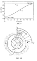
- Fig. 1 is a modeled plot of shear wave velocity as a function of azimuthal angle in an anisotropic formation
- Fig. 2A is a conceptual side view illustration of an acoustic logging system in a borehole environment
- Fig. 2B is a conceptual sectional view of an acoustic logging tool disposed within a borehole and taken through the source section;
- Fig. 3 shows, for a given azimuthal angle segment, a conceptual slowness time coherence (STC) map from a wireline tool comprising a monopole (10 KHz) source in a Bakken shale formation;
- STC slowness time coherence
- Fig. 4 is the semblance projection of the STC map for the angular segment of Fig. 3 ;
- Fig. 5 shows, for a given azimuthal angular segment, a conceptual STC map of from the wireline tool comprising a monopole (10 KHz) source for a Phenolite formation;
- Fig. 6 is the semblance projection of the STC map of Fig. 5 ;
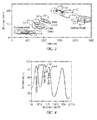
- Fig. 7 illustrates the response of a rotating wireline tool with a low-frequency dipole (2 KHz) source in anisotropic Phenolite formation
- Fig. 8 illustrates the response of the rotating wireline tool with a 2 KHz dipole source in anisotropic Bakken shale formation
- Fig. 9 illustrates the response of the rotating wireline tool with a 2 KHz dipole source in an anisotropic chalk formation
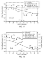
- Fig. 10 illustrates the response of a rotating LWD tool with a 6 KHz unipole source in an anisotropic Bakken shale formation
- Fig. 11 illustrates the response of a rotating LWD tool with a 12 KHz unipole source in an anisotropic limestone formation
- Fig. 12 illustrates the response of a rotating LWD tool with a 6 KHz unipole source in anisotropic chalk formation
- Fig. 13 is a conceptual cross sectional view of a rotating logging tool comprising a unipole or a dipole acoustic source operating at the same relatively high frequency;
- Fig. 14 summarizes the measurement and data processing steps in the form of a conceptual flow chart.
- This invention is a system for measuring acoustic properties of anisotropic earth formation penetrated by a well borehole.
- the system can be embodied as a LWD system in which the source and receiver sections are typically disposed within a drill collar that normally rotates both sections synchronously within the borehole. It is again mentioned that the disclosed LWD apparatus and methods are equally applicable to MWD systems.
- the concepts of the invention can also be embodied as a wireline logging system if the source and receiver sections are synchronously rotated as the wireline tool is conveyed within a borehole.
- the logging systems are designed to operate in, and further to measure anisotrophic properties of the material using a unipole or a dipole acoustic source. Anisotropic measurements are used in a variety of geophysical applications including the correction of other acoustic property measurements used in formation evaluation and seismic applications.
- Transverse isotropy is commonly used to model formation anisotropy.
- the TI anisotropy has a symmetry axis such that material properties and velocities do not vary along any direction transverse to this axis.
- Examples of TI anisotropy are horizontal transverse isotropy (HTI) where the axis of symmetry is horizontal.
- HTI horizontal transverse isotropy
- An example of an HTI formation is anisotropy (caused by fractures, for example) in a plane coincident with the borehole axis in a vertical well.
- VTI vertical transverse isotropy
- An example of a VTI formation is anisotropy along the borehole axis in a vertical well, which is commonly caused by bedding planes.
- Formation anisotropy is defined by a matrix of elastic constants, C, relating the stress to the strain vectors.
- the compressional and shear velocities do not vary with propagation direction and propagate in a direction normal to
- ⁇ the phase angle between the wave front normal and the axis of symmetry.
- Fig. 1 is a plot of ⁇ (abscissa) versus qV SH (ordinate) and shows an example of the expected shear velocity ( qV SH ) profile in an anisotropic formation.
- the curve 12 indicates the velocity of the isotropic rock and curve 14 is the velocity in an anisotropic formation using a model of a water-filled crack with a spatial density of 0.05 and aspect ratio of 0.05.
- Table 1 shows the parameters used to simulate anisotropic formations with different velocities using equations (1) through (8). It is noted that for the chalk formation, the shear velocity is slower than the mud velocity where no refracted shear is detected. The Bakken shale is fast and refracted shear should be detected at any mud velocity. The shear velocity of Phenolite is comparable to the velocity of water and refracted shear is detected only if the mud velocity is higher than roughly 210 us/ft. Table II shows the theoretical shear velocities in these formations.
- FIG. 2A A conceptual side view illustration of an acoustic logging system in a borehole environment is show in Fig. 2A .
- An acoustic borehole instrument or "tool” 20 comprising a source section 23, operating at a frequency of approximately 4 KHz or greater, and a receiver section 22 is shown suspended in a borehole 18 that penetrates earth formation material 21.
- the receiver section 22 comprises a plurality of axially spaced receiver stations R 1 , R 2 , ... R m shown at 24.
- An isolation section 26 is used to minimize direct transmission of acoustic energy from the source section 23 to the receiver section 22.
- the tool 20 is attached to a lower end of conveyance means 32 by a suitable connector 31.
- the upper end of the conveyance means 32 terminates at draw works 34, which is electrically connected to surface equipment 36. Output from the surface equipment 36 cooperates with a recorder 38 that produces a measure, or "log", of one or more parameters of interest as a function of depth within the well borehole.
- a measure, or "log" of one or more parameters of interest as a function of depth within the well borehole.
- the acoustic logging system is a wireline system
- the acoustic tool 20 is a wireline tool
- the conveyance means 32 is a logging cable
- the draw works 34 is a cable winch hoist system that is well known in the art.
- the cable also serves as a data and control conduit between the wireline logging tool 20 and the surface equipment 36.
- the acoustic tool 20 is a acoustic tool typically disposed within a drill collar
- the conveyance means 32 is a drill string
- the draw works 34 is a rotary drilling rig that is well known in the art.
- the tool 20 further comprises an instrument section 33 that comprises power, control, processor and memory elements required to operate the tool.
- the tool 20 also comprises a directional section 29 that is used to measure an "absolute" position of the logging tool 20, as will be discussed in subsequent sections of this disclosure.
- a downhole telemetry element is shown at 28. This is used to telemeter data between the tool 20 and an "uphole" telemetry element (not shown) preferably disposed in the surface equipment 36. These data can include measured acoustic data and computed acoustic parameters. These data can optionally be stored within memory (not shown), preferably disposed within the instrument section 33, for subsequent removal and processing at the surface of the earth 40. Command data for operating the tool 20 can also be telemetered from the surface via the telemetry system.
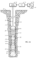
- Fig. 2B is a sectional view of the tool 20 taken through the source section 23 of the tool 20 disposed within the borehole 18.
- the source section 23 (and therefore the tool 20) rotates about the major axis of the tool 20 as indicated conceptually by the arrow 23a.
- An acoustic source which assumed to be a unipole source for purposes of this illustration, is shown at 23b.
- the angle ⁇ is defined by the acoustic wave front normal emitted by the source 23b and the major axis of symmetry of the tool 20.
- a reference angle ⁇ R is defined as 0 degrees for convenience, and azimuthal angle segments ⁇ 1 , ⁇ 2 , ... ⁇ n are shown at 42. These azimuthal angle segments, as well as the "cross-over" angle ⁇ C , will be discussed in subsequent sections of this disclosure.
- This invention is an LWD or a wireline logging system for measuring acoustic properties in anisotrophic properties a unipole or a dipole acoustic source.
- tool 20 was centered (as shown in Fig. 2B ) within a borehole 18 with a 8.5 inch (22.2 centimeters) diameter, and the borehole was filled with 202 us/ft (61.57 us/meter) mud which is fresh water.
- Monopole acoustic sources are not azimuthally directional. Tools with monopole sources can identify formation shear anisotrophy only if the anisotrophy ratio is large enough for the slow and fast shear velocities to register two peaks on a semblance plot projection. For weak anisotropy of 7 percent or less, the shear peaks may not be resolved and the measured shear velocity will be somewhere between the actual fast and slow shear velocities. Moreover, the direction of maximum stress can not be identified using a monopole source.
- the responses of a monopole source tool, operating at 10 KHz, in two modeled formations are presented to illustrate the above mentioned limitations of the monopole source. More specifically, the wireline monopole tool Configuration 1 is used as an example of the data obtained from a monopole source in an anisotropic formation. The source and receiver sections of the wireline tool are rotated synchronously within the borehole. Results and conclusions obtained from the rotating wireline tool can also be applied to an LWD tool with a monopole source.
- Fig. 3 shows, for a given azimuthal segment ⁇ i , a conceptual STC map of the wireline tool monopole data in the Bakken shale formation.
- the STC map has been conceptualized for brevity and comprises a plot of slowness (ordinate) as a function of arrival times from the wave field responses recorded by the receivers 24 shown in Fig. 2A .
- Slowness and arrival times are expressed in units of microseconds per foot (us/ft) and microseconds (ms), respectively, for this and the STC map follows.
- Contours 52, 54 and 56 indicate values of increasing magnitude, respectfully.
- the two arrivals seen in the map are the fast and slow shear velocities which are clearly identified.
- the map also shows the compressional arrival.
- the semblance projection of the STC map for the angular segment of Fig. 3 is shown in Fig. 4 where semblance in percent (ordinate) is plotted as a function of slowness (us/ft).
- the projection shows two distinguished fast shear and slow shear peaks 62 and 64, respectively, falling at 118 and 145 us/ft, which are fairly close to the slow and fast shear velocities of the formation tabulated in Table 2.
- the reason for the two distinguished peaks 62 and 64 in this example is the relatively high anisotropy ratio (20%). If the anisotropy ratio is reduced, the two peaks may not be resolved as illustrated in the following example.
- Fig. 5 shows the STC map, for a given angular segment ⁇ i , of the wireline tool monopole data for the Phenolite formation, which has an anisotropy ratio of 7%.
- the semblance projection of the STC map of Fig. 5 is shown in Fig. 6 .
- the fast and shear arrivals are both within the dashed oval 58 and therefore cannot be resolved on the projection plot.
- the peak value of the arrival depends on the maximum coherence, which happened to be at the fast arrival of 190 us/ft in this case. Other cases may be different and the peak value could be any where between the two velocities depending coherence.
- the monopole source can be used to identify formation fast and slow shear wave slowness, and therefore shear anisotropy, as a function of angular segment ⁇ i , only if the anisotropy ratio is high enough for the slow and fast shear velocities to register two peaks on the semblance plot.
- the slow and fast shear velocity peaks can not be resolved, and the measured shear velocity will be somewhere between the two velocities.
- the direction of maximum stress cannot be identified from monopole sources.
- wireline monopole tool Configuration 1 was used to obtain the above responses of a monopole source in an anisotropic formation. Similar results are obtained by modeling a LWD tool with a monopole source, or an LWD tool with a unipole source after averaging the data from several shots acquired while rotating the tool within the borehole through angle ⁇ .
- Dipole and unipole sources are azimuthally directional and are therefore conceptually suited for measuring azimuthal anisotrophy.
- Wireline tools comprising crossed dipole acoustic sources have been used in the prior art to measure formation anisotropy. Details of a cross dipole anisotropy wireline system are disclosed in U.S. Patent Nos: 5,343,441 ; 7,310,285 B2 ; 7,646,674 B2 ; and 6.098,021 , which are incorporated herein by reference.
- a wireline tool typically does not rotate as it is conveyed along the borehole.
- Mechanical means can, in principle, be embodied to synchronously rotate (at least) the source and receiver and receiver sections in order to obtain the desired anisotropy sensitivity of this invention.
- Anisotropy measurements from a low frequency dipole source in a wireline tool are typically made using what is known as crossed-dipole measurements.
- crossed-dipole measurements are made using two sets of orthogonal dipole transmitters disposed within the source section 23, and with each receiver station 24 comprising orthogonal receivers. This is the previously described wireline Configuration 2.
- the orthogonal transmitters and receivers are azimuthally aligned.
- Waveform data are collected in the inline and cross-line receivers from the orthogonal transmitters to form four waveform data sets usually referred to as XX, YY (inline) and XY and YX (cross-line).
- a mathematical rotation commonly known as Alford Rotation, shown in U.S. Patent No. 5,343,441 , which is incorporated herein by reference. is then applied to the four sets of data to obtain the slow and fast velocities and the direction of maximum stress.
- Fig. 7 The response, in anisotropic Phenolite, of a rotating wireline tool with a low-frequency dipole (2 KHz) is shown in Fig. 7 .
- the illustration is a plot of shear slowness (us/ft) as a function of azimuthal angle of tool rotation ⁇ (degrees).
- the "theoretical" curve 62 represents the response calculated using equations (1) - (8) and "measured" tool shear velocities modeled in 15 degree azimuthal segments ⁇ i are identified as 64.
- Fig. 7 shows a fairly good agreement measured values 64 and the theoretical values represented by the curve 62. Illustrations of corresponding STC maps and corresponding semblance projections have been omitted for brevity.
- Fig. 8 is a plot of shear slowness as a function of ⁇ .
- the curve 63 represents the theoretical response calculated using equations (1) - (8) and measured tool shear velocities modeled in 15 degree azimuthal segments ⁇ i are identified as 65.
- the overall higher measured slowness compared to the theoretical slowness 63 is to due to dispersion effects. This is more noticeable for the Bakken shale case given the fast shear velocity arriving at a relatively high frequency (3-4 KHz).
- Fig. 9 is a plot of shear slowness as a function of ⁇ .
- the curve 67 represents the theoretical response calculated using equations (1) - (8) and "measured" tool shear velocities modeled in 15 degree azimuthal segments ⁇ i are identified as 69 shows.
- the overall higher measured slowness 69 compared to the theoretical slowness 67 is to due to dispersion effects.
- Unipole acoustic sources emit energy pulses that are azimuthally directional.
- the following results are obtained using a unipole source disposed within a LWD tool such that the emitted pulse is essentially orthogonal to the major axis of the tool.
- a conceptual illustration of the unipole source disposition is illustrated at 23b in Fig. 2B .
- acoustic receivers disposed within axially spaced receiver stations 24 shown in Fig. 2A are preferably azimuthally aligned with the unipole source. This is the previously defined LWD Configuration 3.
- An LWD logging tool comprising a dipole source operating in the 6 and 12 KHz range can be used in a drilling environment.
- Modeling results show no significant difference in tool response employing a high frequency dipole source and a unipole source operating at the same frequency.
- results in the following section are given for a unipole acoustic source, the same results are applicable to a LWD tool operating at the same frequency and are so indicated in the following illustrations.
- Fig. 10 illustrates the response of a rotating LWD tool with a 6 KHz unipole source in anisotropic Bakken shale formation.
- Fig. 10 is a plot of shear slowness as a function of angle ⁇ .
- the curve 63 represents the response calculated using equations (1) - (8) and is essentially identical to the results for the 2 KHz dipole wireline tool shown in Fig. 8 .
- the measured shear velocities modeled in 15 degree azimuthal segments ⁇ i are identified as 65 are for the 2 KHz dipole wireline tool and are shown for reference.
- the measured shear velocities modeled in 15 degree azimuthal segments ⁇ i are identified as 70 are for the 6 KHz unipole LWD tool.
- the measurements 70 are shown to represent both embodiments.
- This angle 72 is defined as the "cross-over" angle and is hereafter denoted as ⁇ C .
- Fig. 11 is a plot of shear slowness as a function of ⁇ .
- Data points 64 have been previously discussed and function in this discussion as reference measurements from the rotating wireline tool with a dipole source operating at 2 KHz.
- the curve 74 represents the theoretical response calculated using equations (1) - (8).
- the measured shear velocities modeled in 15 degree azimuthal segments ⁇ i are identified as 78 are for a 12 KHz unipole LWD tool as well as a 12 KHz dipole wireline tool.
- Fig. 12 is a plot of shear slowness as a function of ⁇ i in an anisotropic chalk formation. Recall that the chalk formation is relatively slow (see Table 2).
- Data points 69 are the reference measurements from the rotating wireline tool with a dipole source operating at 2 KHz and are the same as those shown in Fig. 9 .
- the curve 67 represents the response calculated using equations (1) - (8) and is likewise the same as the theoretical curve shown in Fig. 9 .
- the measured shear velocities modeled in 15 degree azimuthal segments ⁇ i are identified as 80 are for the 6 KHz unipole LWD tool and also representative of the response for a 6 KHz dipole wireline tool.
- Fig. 13 is a conceptual cross sectional view of a rotating logging tool comprising a unipole or dipole acoustic source operating at the same relatively high frequency.
- the angle of the fast-slow boundary is referenced to an absolute reference angle ⁇ ABS which can be magnetic north, the "high" side of a deviated borehole, and the like.
- LWD unipole measurements made at higher frequencies can provide the slow and fast formation velocities with good accuracy in fast formations.
- the direction of minimum/maximum stress can be determined from these measurements by detecting the angle at which the velocity changes from fast to slow, which is defined as the cross-over angle.
- the direction of maximum stress is 45 degrees (relative to the tool reference angle) from the cross-over angle towards the slow velocity and the direction of minimum stress is 45 degrees.
- Fig. 14 summarizes the measurement and data processing methods in the form of a conceptual flow chart. Specific identifiers from Figs. 2A , 2B and 13 are also referenced.
- the acoustic source within the source section 23 is fired at step 90.
- the wave field generated by the acoustic pulse is received by plurality of detectors in the receiver section 24. These waveforms are digitized by a suitable analog to digital converter typically disposed within the instrument section 33 of the logging tool 20. These operations are indicated at step 92.
- Measured waveform data are partitioned at step 94 into azimuthal angle segments ⁇ i as the tool rotates within the borehole.
- shear velocity is computed for each azimuthal angle segments ⁇ i as described in previous sections of this disclosure.
- a cross-over angle cross-over angle ⁇ C if present, is determined at step 98.
- Steps 90 through 98 are repeated for each source section-receiver section revolution within the borehole.
- the cross-over angle ⁇ C is related at step 100 to an absolute reference angle ⁇ ABS using output from a directional section 29.
- the absolute reference angle can be magnetic north, the high side of a deviated borehole, and the like.
- anisotropic formation parameters and other parameters of interest (POI) using the previously described measured and computed data.
- Parameters of interest are recorded at step 104 as a function of depth. These parameters of interest can be recorded in memory disposed within the instrument section 33 for subsequent retrieval at the surface of the earth surface 40.
- parameters of interest can be telemetered to the surface via the telemetry system 31, received by surface equipment 31, recorded in a surface recorder 38 which generates a "log" 39 of the parameters of interest as a function of depth.
- depth is incremented and steps 90 through 104 are repeated thereby generating the log 39.
- the measure of acoustic properties of anisotropic formations penetrated by a borehole can be summarized as follows: of material penetrated by a well borehole
Landscapes
- Physics & Mathematics (AREA)
- Life Sciences & Earth Sciences (AREA)
- Engineering & Computer Science (AREA)
- Acoustics & Sound (AREA)
- Environmental & Geological Engineering (AREA)
- Geology (AREA)
- Remote Sensing (AREA)
- General Life Sciences & Earth Sciences (AREA)
- General Physics & Mathematics (AREA)
- Geophysics (AREA)
- Geophysics And Detection Of Objects (AREA)
- Earth Drilling (AREA)
Abstract
Description
- This invention is related to systems for measuring one or more acoustic properties of material penetrated by a well borehole. More particularly, the invention is related to measuring anisotrophic properties of the material using unipole and dipole acoustic sources. Anisotropic measurements are used in a variety of geophysical applications.
- Acoustic logging systems are routinely used in the oil and gas industry to measure formation acoustic properties of earth formation penetrated by a well borehole. These properties include the compressional and shear velocities of the formation, which are subsequently used to determine a variety of formation parameters of interest including, but not limited to; porosity, lithology, density and pore pressure. Additionally, acoustic logging systems are used to produce acoustic images of the borehole from which well conditions and other geological features can be investigated. Other applications of acoustic logging measurements include seismic correlation and rock mechanic determination.
- The above mentioned acoustic measurements typically need to be corrected for any formation anisotrophic effects before parameters of interest can be determined from the measured parameters. Furthermore, anisotrophy parameters are themselves parameters of interest, and are used in a variety of geophysical applications including cross-well seismic measurements, convention seismic interpretations, and the like. Elastic anisotropy manifests itself as the directional dependence of sound speed in earth formation. Anisotropy in earth formation may be due to intrinsic microstructure, such as the case in shales, or may be due to mesostructure, such as fractures, or may be due to macrostructure such as layering due to sedimentation. Whatever the cause for anisotropy may be, good estimates of elastic properties of anisotropic media are required in resolving seismic images accurately, in interpreting borehole logs and in estimating drilling mechanics parameters.
- Most formations have anisotropic structure resulting from layering, micro fractures, or orientation of mineral deposits in a certain direction. This internal stress causes the shear velocity to vary with propagation direction. Transverse isotropy (TI) is commonly used to model formation anisotropy. One example of TI anisotropy is horizontal transverse isotropy (HTI) where the axis of anisotropic symmetry is horizontal. Another example of TI anisotropy is vertical transverse isotropy, where the axis of anisotropic symmetry is vertical. Specific examples of these TI anisotropy formations are vertical fracturing along the borehole axis and horizontal bedding planes in a vertical well.
- Formation anisotropy can be determined with acoustic logging-while-drilling (LWD) or measurement-while-drilling (MWD) systems. Formation anisotropy can also be determined with acoustic wireline systems after the borehole drilling operation is complete. MWD, LWD, and wireline acoustic logging systems comprising monopole and dipole acoustic sources have been used in the prior art as shown, for example, in
U.S. Patent Nos. 7,623,412 B2 ,5,808,963 ,6,714,480 B2 ,7,310,285 B2 ,7,646,674 B2 , which are incorporated herein by reference. There are operational and environment factors that limit practical source frequencies, especially in MWD and LWD systems. This topic will be discussed in detail in subsequent sections of this disclosure. - This invention is based upon anisotropic formation modeling and acoustic logging system tool response modeling in anisotropic formations. The invention can be embodied as a MWD, LWD or wireline logging system. Hereafter, all systems that measure parameters of interest while drilling will be referred to as "LWD" systems, although it should be understood the invention can also be embodied as a MWD system. LWD and wireline logging systems comprising a unipole or alternately a dipole acoustic source are developed from the modeling. The borehole instrument or "logging tool" comprises a source section and a receiver section. The source section comprises a source of acoustic energy operated at a frequency of approximately 4 kilohertz (KHz) or greater for the LWD or MWD tool and 1 KHz or greater for the wireline tool. The receiver section comprises a plurality of receiver stations axially spaced at different distances from the acoustic source. An isolator section isolates the source and receiver sections from direct acoustic transmission. The logging tool also comprises an instrument section comprising power, processor, memory and control elements, a downhole telemetry section, and a directional section that yields the absolute orientation of the logging tool. In addition to the logging tool, the logging system comprises a conveyance means, draw works, surface equipment comprising a surface telemetry element, and a surface recorder. All system elements will be described in detail in subsequent sections of this disclosure. The source and receiver sections of the logging tool rotate azimuthally as the logging tool is conveyed along the well borehole.
- Acoustic logging system responses are presented for three basic system configurations in a variety of anisotrophic formations. The first response modeling is for a wireline tool comprising a monopole acoustic source operating at a frequency of 10 KHz, and further comprising six receiver stations at six different axial spacings from the source, wherein each station comprising one monopole acoustic receiver. The second response modeling is for a wireline tool comprising a dipole acoustic source operating at 2 KHz, and further comprising eight receiver stations at eight different axial spacings from the source and with each station comprising two directional acoustic receivers at 180 degrees from each other. The third response modeling is for a LWD tool that comprises a single sided unipole acoustic source operating at 6 and 12 KHz, and further comprising six receiver stations at six different axial spacings from the source with each station comprising one directional acoustic receiver lined up with the source. It is noted that additional modeling was made for a LWD tool comprising a dipole source with a receiver array that is configured the same as the third response model defined above. Response results from the dipole LWD tool, operating at the same frequency as the third (unipole) response model, were essentially the same as the third response model comprising the unipole source. Details of the LWD "high frequency" dipole model results have, therefore, been omitted from this disclosure for brevity but are included in the analysis of the system response results.
- In each of the above configurations, model response results were obtained for the acoustic source and receiver sections rotating synchronously about the major axis of the borehole in an HTI anisotropic formation. It was assumed that the formation anisotropy is azimuthally symmetric around the wall of the borehole. Waveform data were generated in contiguous azimuthal angle segments Δθ i = 15 degrees in the range of 0 to 90 degrees (i.e. i = 1, 2, ... , 6). Time-slowness coherence analysis (STC) was used to determine the shear velocity in each azimuthal angle segments Δθ i . Other methods such as maximum likelihood or slowness frequency coherence analysis can be used to determine the formation velocities.
- The operation procedures for the acoustic logging system, whether LWD or wireline, are summarized as follows. The logging tool, with synchronously rotating source and receiver sections, is conveyed along the borehole. The acoustic source within the source section is fired periodically as the source section rotates. The acoustic wave field generated by the acoustic pulse is received by the plurality of detectors in the receiver section. These waveforms are conditioned and digitized using an analog to digital converter typically disposed within the instrument section of the logging tool. Measured waveform data are partitioned into azimuthal angle segments Δθ i for each 360 degree revolution of the source and receiver sections. Shear velocity is computed for each azimuthal angle segments Δθ i . A cross-over angle segments Δθ C , if present, is determined from the Δθ i along with a corresponding cross-over angle θ C . The above steps are repeated for each source section-receiver section revolution within the borehole. For each revolution, the cross-over angle θ C is related to an absolute reference angle θ ABS using output from a directional section of the logging tool. The absolute reference angle can be magnetic north, the high side of a deviated borehole, and the like. Anisotropic formation parameters and other parameters of interest (POI) are obtained from measured and computed data. Depth of the tool in the borehole and the above steps are repeated. Parameters of interest are recorded as a function of depth of the logging tool within the borehole thereby generating a "log" of the parameters of interest.
- The manner in which the above recited features and advantages, briefly summarized above, are obtained can be understood in detail by reference to the embodiments illustrated in the appended drawings.
-
Fig. 1 is a modeled plot of shear wave velocity as a function of azimuthal angle in an anisotropic formation; -
Fig. 2A is a conceptual side view illustration of an acoustic logging system in a borehole environment; -
Fig. 2B is a conceptual sectional view of an acoustic logging tool disposed within a borehole and taken through the source section; -
Fig. 3 shows, for a given azimuthal angle segment, a conceptual slowness time coherence (STC) map from a wireline tool comprising a monopole (10 KHz) source in a Bakken shale formation; -
Fig. 4 is the semblance projection of the STC map for the angular segment ofFig. 3 ; -
Fig. 5 shows, for a given azimuthal angular segment, a conceptual STC map of from the wireline tool comprising a monopole (10 KHz) source for a Phenolite formation; -
Fig. 6 is the semblance projection of the STC map ofFig. 5 ; -
Fig. 7 illustrates the response of a rotating wireline tool with a low-frequency dipole (2 KHz) source in anisotropic Phenolite formation; -
Fig. 8 illustrates the response of the rotating wireline tool with a 2 KHz dipole source in anisotropic Bakken shale formation; -
Fig. 9 illustrates the response of the rotating wireline tool with a 2 KHz dipole source in an anisotropic chalk formation; -
Fig. 10 illustrates the response of a rotating LWD tool with a 6 KHz unipole source in an anisotropic Bakken shale formation; -
Fig. 11 illustrates the response of a rotating LWD tool with a 12 KHz unipole source in an anisotropic limestone formation; -
Fig. 12 illustrates the response of a rotating LWD tool with a 6 KHz unipole source in anisotropic chalk formation; -
Fig. 13 is a conceptual cross sectional view of a rotating logging tool comprising a unipole or a dipole acoustic source operating at the same relatively high frequency; and -
Fig. 14 summarizes the measurement and data processing steps in the form of a conceptual flow chart. - This invention is a system for measuring acoustic properties of anisotropic earth formation penetrated by a well borehole. The system can be embodied as a LWD system in which the source and receiver sections are typically disposed within a drill collar that normally rotates both sections synchronously within the borehole. It is again mentioned that the disclosed LWD apparatus and methods are equally applicable to MWD systems. The concepts of the invention can also be embodied as a wireline logging system if the source and receiver sections are synchronously rotated as the wireline tool is conveyed within a borehole. The logging systems are designed to operate in, and further to measure anisotrophic properties of the material using a unipole or a dipole acoustic source. Anisotropic measurements are used in a variety of geophysical applications including the correction of other acoustic property measurements used in formation evaluation and seismic applications.
- The responses of the unipole and dipole LWD and wireline systems are illustrated by formation and tool response modeling.
- Modeling of Anisotropic Formations
- As mentioned previously, most earth formations or "rocks" have anisotropic structure resulting from layering, micro fractures, or orientation of mineral deposits in a certain direction. This internal stress causes the shear velocity to vary with propagation direction. Transverse isotropy (TI) is commonly used to model formation anisotropy. The TI anisotropy has a symmetry axis such that material properties and velocities do not vary along any direction transverse to this axis. Examples of TI anisotropy are horizontal transverse isotropy (HTI) where the axis of symmetry is horizontal. An example of an HTI formation is anisotropy (caused by fractures, for example) in a plane coincident with the borehole axis in a vertical well. Another example of TI anisotropy is vertical transverse isotropy (VTI), where the axis of symmetry is vertical. An example of a VTI formation is anisotropy along the borehole axis in a vertical well, which is commonly caused by bedding planes.
- The following formalism is used to compute idealized or "theoretical" acoustic tool responses in anisotropic formations. Formation anisotropy is defined by a matrix of elastic constants, C, relating the stress to the strain vectors. The matrix of the elastic constants has nine independent coefficients as shown in the following equation:

In an isotropic formation;


where λ and µ are the Lamé bulk and shear constants of the medium. In an isotropic medium, the compressional and shear velocities do not vary with propagation direction and propagate in a direction normal to the tangent of the wave front. - In an anisotropic formation, the velocity varies with propagation direction. In a transversely isotropic formation, which is a common representation of an anisotropic medium, the quasi compressional velocity, qVP, is given by

The quasi shear velocity, qVSV, is given by
and the shear velocity, qVSH , is given by
where
ρ = the density of the formation, and
θ = the phase angle between the wave front normal and the axis of symmetry. -
Fig. 1 is a plot of θ (abscissa) versus qVSH (ordinate) and shows an example of the expected shear velocity (qVSH ) profile in an anisotropic formation. Thecurve 12 indicates the velocity of the isotropic rock andcurve 14 is the velocity in an anisotropic formation using a model of a water-filled crack with a spatial density of 0.05 and aspect ratio of 0.05. - Table 1 shows the parameters used to simulate anisotropic formations with different velocities using equations (1) through (8). It is noted that for the chalk formation, the shear velocity is slower than the mud velocity where no refracted shear is detected. The Bakken shale is fast and refracted shear should be detected at any mud velocity. The shear velocity of Phenolite is comparable to the velocity of water and refracted shear is detected only if the mud velocity is higher than roughly 210 us/ft. Table II shows the theoretical shear velocities in these formations.
Table 1 Formation Properties used for Modeling HTI anisotropy Model Density (g/cc) C11 (GPa) C12 =C13 (GPa) C22=C33 (GPa) C23 (GPa) C44 (GPa) C55 =C66 (GPa) Phenolite 1.32 10.58 5.71 13.61 6.68 3.42 2.97 Bakken Shale 2.23 26.9 8.5 42.9 12.35 15.3 10.5 Chalk 2.19 14 12 22 15.8 3.1 2.4 Table 2 Formation Slow and Fast Shear Velocities for the Modeled HTI anisotropy Model Slow Shear (us/ft) Fast Shear (us/ft) Phenolite 202.27 189.36 Bakken Shale 138.01 116.36 Chalk 289.09 256.46 - Modeling of Acoustic Tool Response in Anisotropic Formations
- Responses of various acoustic logging systems were modeled in anisotropic formations, in a well borehole environment, using a finite difference model. These model results are used to determine optimum parameters for determining anisotropic properties of interest, and to illustrate the advantages of rotating LWD and wireline systems using a unipole or a dipole acoustic source operating at relatively high frequencies.
- A conceptual side view illustration of an acoustic logging system in a borehole environment is show in
Fig. 2A . An acoustic borehole instrument or "tool" 20 comprising asource section 23, operating at a frequency of approximately 4 KHz or greater, and areceiver section 22 is shown suspended in a borehole 18 that penetratesearth formation material 21. Thereceiver section 22 comprises a plurality of axially spaced receiver stations R1, R2, ... Rm shown at 24. Anisolation section 26 is used to minimize direct transmission of acoustic energy from thesource section 23 to thereceiver section 22. Thetool 20 is attached to a lower end of conveyance means 32 by asuitable connector 31. The upper end of the conveyance means 32 terminates at draw works 34, which is electrically connected to surfaceequipment 36. Output from thesurface equipment 36 cooperates with arecorder 38 that produces a measure, or "log", of one or more parameters of interest as a function of depth within the well borehole. If the acoustic logging system is a wireline system, theacoustic tool 20 is a wireline tool, the conveyance means 32 is a logging cable, and the draw works 34 is a cable winch hoist system that is well known in the art. The cable also serves as a data and control conduit between thewireline logging tool 20 and thesurface equipment 36. If the acoustic logging system is a LWD system, theacoustic tool 20 is a acoustic tool typically disposed within a drill collar, the conveyance means 32 is a drill string, and the draw works 34 is a rotary drilling rig that is well known in the art. - Still referring to
Fig. 2A , thetool 20 further comprises aninstrument section 33 that comprises power, control, processor and memory elements required to operate the tool. Thetool 20 also comprises adirectional section 29 that is used to measure an "absolute" position of thelogging tool 20, as will be discussed in subsequent sections of this disclosure. A downhole telemetry element is shown at 28. This is used to telemeter data between thetool 20 and an "uphole" telemetry element (not shown) preferably disposed in thesurface equipment 36. These data can include measured acoustic data and computed acoustic parameters. These data can optionally be stored within memory (not shown), preferably disposed within theinstrument section 33, for subsequent removal and processing at the surface of theearth 40. Command data for operating thetool 20 can also be telemetered from the surface via the telemetry system. -
Fig. 2B is a sectional view of thetool 20 taken through thesource section 23 of thetool 20 disposed within theborehole 18. The source section 23 (and therefore the tool 20) rotates about the major axis of thetool 20 as indicated conceptually by thearrow 23a. An acoustic source, which assumed to be a unipole source for purposes of this illustration, is shown at 23b. The angle θ is defined by the acoustic wave front normal emitted by thesource 23b and the major axis of symmetry of thetool 20. A reference angle θ R is defined as 0 degrees for convenience, and azimuthal angle segments Δθ 1 , Δθ 2 , ... Δθ n are shown at 42. These azimuthal angle segments, as well as the "cross-over" angle Δθ C , will be discussed in subsequent sections of this disclosure. - Response Model Results
- This invention is an LWD or a wireline logging system for measuring acoustic properties in anisotrophic properties a unipole or a dipole acoustic source.
- Again referring to
Figs. 2A and2B , responses of acoustic logging systems in anisotropic formations were modeled for the following configurations: - Configuration 1: A
wireline tool 20 with:- (a) a monopole acoustic source operating at 10 KHz and disposed in the
source section 23; and - (b) six
receiver stations 24 with each station comprising one acoustic receiver.
- (a) a monopole acoustic source operating at 10 KHz and disposed in the
- Configuration 2: A
wireline tool 20 with- (a) a dipole acoustic source operating at 2 KHz and disposed in the
source section 23; and - (b) eight
receiver stations 24 with each station comprising two acoustic receivers.
- (a) a dipole acoustic source operating at 2 KHz and disposed in the
- Configuration 3: An
LWD tool 20 that is 6.75 inches (17.2 centimeters) in diameter and with- (a) a single sided unipole acoustic source operating at 6 and 12 KHz and disposed in the
source section 23; and - (b) six
receiver stations 24 with each station comprising one acoustic receiver.
- (a) a single sided unipole acoustic source operating at 6 and 12 KHz and disposed in the
- For each of the above configurations,
tool 20 was centered (as shown inFig. 2B ) within aborehole 18 with a 8.5 inch (22.2 centimeters) diameter, and the borehole was filled with 202 us/ft (61.57 us/meter) mud which is fresh water. - In each of the above configurations, model response results were obtained for the
logging tool 20 tool rotating about the major axis of theborehole 18 and in an HTI anisotropic formation. It was assumed that the anisotropy is azimuthally symmetric. Waveform data were generated in contiguous azimuthal angle segments Δθ i = 15 degrees in the range of 0 to 90 degrees (i.e. i = 1, 2, ... , 6) using previously defined nomenclature. Again Δθ R = 0 degrees is defined as the tool azimuthal reference angle. Time-slowness coherence analysis (STC) was used to determine the shear velocity. Shear velocities were computed from the semblance projection at each angle and compared to their theoretical values. - Response Model Results-Monopole Sources
- Monopole acoustic sources are not azimuthally directional. Tools with monopole sources can identify formation shear anisotrophy only if the anisotrophy ratio is large enough for the slow and fast shear velocities to register two peaks on a semblance plot projection. For weak anisotropy of 7 percent or less, the shear peaks may not be resolved and the measured shear velocity will be somewhere between the actual fast and slow shear velocities. Moreover, the direction of maximum stress can not be identified using a monopole source.
- The responses of a monopole source tool, operating at 10 KHz, in two modeled formations are presented to illustrate the above mentioned limitations of the monopole source. More specifically, the wireline
monopole tool Configuration 1 is used as an example of the data obtained from a monopole source in an anisotropic formation. The source and receiver sections of the wireline tool are rotated synchronously within the borehole. Results and conclusions obtained from the rotating wireline tool can also be applied to an LWD tool with a monopole source. - The results of a monopole source were similar for all modeled tool responses. Since the monopole data do not change significantly while the tool is rotating in the borehole, the model at any rotational angle produced essentially the same results.
-
Fig. 3 shows, for a given azimuthal segment Δθ i , a conceptual STC map of the wireline tool monopole data in the Bakken shale formation. The STC map has been conceptualized for brevity and comprises a plot of slowness (ordinate) as a function of arrival times from the wave field responses recorded by thereceivers 24 shown inFig. 2A . Slowness and arrival times are expressed in units of microseconds per foot (us/ft) and microseconds (ms), respectively, for this and the STC map follows.Contours - The semblance projection of the STC map for the angular segment of
Fig. 3 is shown inFig. 4 where semblance in percent (ordinate) is plotted as a function of slowness (us/ft). The projection shows two distinguished fast shear and slow shear peaks 62 and 64, respectively, falling at 118 and 145 us/ft, which are fairly close to the slow and fast shear velocities of the formation tabulated in Table 2. However, the reason for the twodistinguished peaks -
Fig. 5 shows the STC map, for a given angular segment Δθ i , of the wireline tool monopole data for the Phenolite formation, which has an anisotropy ratio of 7%. The fast and slow shear velocities, inclosed in the dashedoval 57, are not clearly identified. The semblance projection of the STC map ofFig. 5 is shown inFig. 6 . In this formation, the fast and shear arrivals are both within the dashedoval 58 and therefore cannot be resolved on the projection plot. The peak value of the arrival depends on the maximum coherence, which happened to be at the fast arrival of 190 us/ft in this case. Other cases may be different and the peak value could be any where between the two velocities depending coherence. - Using the two models of a wireline tool comprising a monopole source, the following conclusions are apparent. The monopole source can be used to identify formation fast and slow shear wave slowness, and therefore shear anisotropy, as a function of angular segment Δθ i , only if the anisotropy ratio is high enough for the slow and fast shear velocities to register two peaks on the semblance plot. However, for typical weak anisotropy of 7% of less, the slow and fast shear velocity peaks can not be resolved, and the measured shear velocity will be somewhere between the two velocities. Moreover, the direction of maximum stress cannot be identified from monopole sources. It is again emphasized that the wireline
monopole tool Configuration 1 was used to obtain the above responses of a monopole source in an anisotropic formation. Similar results are obtained by modeling a LWD tool with a monopole source, or an LWD tool with a unipole source after averaging the data from several shots acquired while rotating the tool within the borehole through angle θ. - Response Model Results-Dipole and Unipole Sources
- Dipole and unipole sources are azimuthally directional and are therefore conceptually suited for measuring azimuthal anisotrophy.
- Wireline tools comprising crossed dipole acoustic sources have been used in the prior art to measure formation anisotropy. Details of a cross dipole anisotropy wireline system are disclosed in
U.S. Patent Nos: 5,343,441 ;7,310,285 B2 ;7,646,674 B2 ; and6.098,021 , which are incorporated herein by reference. A wireline tool typically does not rotate as it is conveyed along the borehole. Mechanical means can, in principle, be embodied to synchronously rotate (at least) the source and receiver and receiver sections in order to obtain the desired anisotropy sensitivity of this invention. - While the conclusions made for monopole sources can be applied equally to wireline and LWD tools, acoustic signals from dipole sources are vastly different when used while drilling. One of the main differences is not being able to operate a dipole source at low frequency while drilling because of interference from the drilling noise. Operating a dipole source at high frequencies (4-8 KHz) requires much larger dispersion corrections than when operating at low frequencies (1-2 KHz). Second, the mass and stiffness of the drill collar affects the dipole measurements while drilling, which makes the measurement made from an LWD tool at 4-8 KHz only marginally better than the one obtained from a single-sided monopole (unipole) source.
- Wireline Dipole Source
- Anisotropy measurements from a low frequency dipole source in a wireline tool are typically made using what is known as crossed-dipole measurements. Referring again to
Figs 2A and2B , crossed-dipole measurements are made using two sets of orthogonal dipole transmitters disposed within thesource section 23, and with eachreceiver station 24 comprising orthogonal receivers. This is the previously describedwireline Configuration 2. The orthogonal transmitters and receivers are azimuthally aligned. Waveform data are collected in the inline and cross-line receivers from the orthogonal transmitters to form four waveform data sets usually referred to as XX, YY (inline) and XY and YX (cross-line). A mathematical rotation, commonly known asAlford Rotation, shown in U.S. Patent No. 5,343,441 , which is incorporated herein by reference. is then applied to the four sets of data to obtain the slow and fast velocities and the direction of maximum stress. - In theory, the shear measurements from a mechanically rotating dipole wireline tool should track the theoretical values shown in
Fig. 1 . The response, in anisotropic Phenolite, of a rotating wireline tool with a low-frequency dipole (2 KHz) is shown inFig. 7 . The illustration is a plot of shear slowness (us/ft) as a function of azimuthal angle of tool rotation θ (degrees). The "theoretical"curve 62 represents the response calculated using equations (1) - (8) and "measured" tool shear velocities modeled in 15 degree azimuthal segments Δθ i are identified as 64.Fig. 7 shows a fairly good agreement measuredvalues 64 and the theoretical values represented by thecurve 62. Illustrations of corresponding STC maps and corresponding semblance projections have been omitted for brevity. - The response of the rotating wireline tool formation with a 2 KHz dipole source in anisotropic Bakken shale is shown in
Fig. 8 . As inFig. 7, Fig. 8 is a plot of shear slowness as a function of θ. Thecurve 63 represents the theoretical response calculated using equations (1) - (8) and measured tool shear velocities modeled in 15 degree azimuthal segments Δθ i are identified as 65. STC maps (not shown) at azimuthal segments Δθ i = 45 degrees and 60 degrees indicate that the shear velocity arrivals can not be resolved, therefore measuredvalues 65 in these azimuthal segments have been omitted. The overall higher measured slowness compared to thetheoretical slowness 63 is to due to dispersion effects. This is more noticeable for the Bakken shale case given the fast shear velocity arriving at a relatively high frequency (3-4 KHz). - The response of the rotating wireline tool formation with a 2 KHz dipole source in anisotropic chalk formation is shown in
Fig. 9 . Once again,Fig. 9 is a plot of shear slowness as a function of θ. Thecurve 67 represents the theoretical response calculated using equations (1) - (8) and "measured" tool shear velocities modeled in 15 degree azimuthal segments Δθ i are identified as 69 shows. An STC map (not shown) at azimuthal segments Δθ i = 60 degrees indicates that fast and shear velocity arrivals can not be resolved, therefore measuredvalues 69 in this azimuthal segment has been omitted. As in the case of the Bakken shale, the overall higher measuredslowness 69 compared to thetheoretical slowness 67 is to due to dispersion effects. - Given that the above rotating wireline dipole data tracks the theoretical velocity profile while rotating, several anisotropy parameters can be determined from the data:
- 1. The slow and fast shear velocities can be determined as the minimum and maximum velocities measured while rotating;
- 2. The anisotropy ratio can be readily calculated from the minimum and maximum shear velocities; and
- 3. The directions of maximum/minimum stresses can also be readily calculated from the angles at which the minim and maximum velocities are measured.
- To summarize, low frequency crossed-dipole measurements from wireline tools are well established, but due to the previously noted reasons, they cannot be applied to a LWD acoustic system. Therefore, there is a need for a method of detecting anisotropy while drilling. Given that LWD tools rotate most of the time, a new principle based on a rotating unipole tool is introduced in the following section.
- The LWD Unipole and Dipole Acoustic Logging System
- Unipole acoustic sources emit energy pulses that are azimuthally directional. The following results are obtained using a unipole source disposed within a LWD tool such that the emitted pulse is essentially orthogonal to the major axis of the tool. A conceptual illustration of the unipole source disposition is illustrated at 23b in
Fig. 2B . Furthermore, acoustic receivers disposed within axially spacedreceiver stations 24 shown inFig. 2A are preferably azimuthally aligned with the unipole source. This is the previously defined LWD Configuration 3. - An LWD logging tool comprising a dipole source operating in the 6 and 12 KHz range can be used in a drilling environment. Modeling results show no significant difference in tool response employing a high frequency dipole source and a unipole source operating at the same frequency. Although results in the following section are given for a unipole acoustic source, the same results are applicable to a LWD tool operating at the same frequency and are so indicated in the following illustrations.
- In fast formations where refracted shear waves are detected from a unipole source, the velocity profile obtained from a rotating unipole tool agrees with the theoretical values at the fast and slow directions, and changes fairly abruptly from one velocity to the other velocity at θ = 45 degrees. This trend can be seen in
Fig. 10 . More specifically,Fig. 10 illustrates the response of a rotating LWD tool with a 6 KHz unipole source in anisotropic Bakken shale formation. Once again,Fig. 10 is a plot of shear slowness as a function of angle θ. As stated previously, modeling of a rotating wireline tool with a dipole source operating at 6 KHz yielded essentially the same results as a rotating LWD tool with a dipole source operating at 6 KHz. The higher 6 KHz frequency is operational feasible in a drilling environment as previously discussed. Thecurve 63 represents the response calculated using equations (1) - (8) and is essentially identical to the results for the 2 KHz dipole wireline tool shown inFig. 8 . The measured shear velocities modeled in 15 degree azimuthal segments Δθ i are identified as 65 are for the 2 KHz dipole wireline tool and are shown for reference. The measured shear velocities modeled in 15 degree azimuthal segments Δθ i are identified as 70 are for the 6 KHz unipole LWD tool. As mentioned previously, essentially identical results were obtained for a rotating wireline tool with a 6 KHz source, therefore themeasurements 70 are shown to represent both embodiments. The measured values 70 are relatively constant on either side of Δθ i = 45 degrees as indicated by the broken horizontal lines. There is an abrupt change in shear slowness at θ = 45 degrees. Thisangle 72 is defined as the "cross-over" angle and is hereafter denoted as θ C . The abrupt change at θ C . = 45 degrees does, therefore, define the azimuthal position of the change in shear wave velocity and thus a relative azimuthal direction for shear anisotrophy. - The abrupt change in shear arrival shown in the Bakken shale was confirmed by similar modeling in a limestone formation with 5 percent HTI anisotrophy. These results are shown in
Fig. 11 . Again,Fig. 11 is a plot of shear slowness as a function of θ. Data points 64 have been previously discussed and function in this discussion as reference measurements from the rotating wireline tool with a dipole source operating at 2 KHz. Thecurve 74 represents the theoretical response calculated using equations (1) - (8). The measured shear velocities modeled in 15 degree azimuthal segments Δθ i are identified as 78 are for a 12 KHz unipole LWD tool as well as a 12 KHz dipole wireline tool. As in the previous illustration, the measuredvalues 78 are relatively constant on either side of θ = 45 degrees as indicated by the broken lines. An abrupt change occurs again at θ C . = 45 degrees thereby defining the azimuthal position of the change in shear wave velocity and thus a relative azimuthal direction for shear anisotrophy. -
Fig. 12 is a plot of shear slowness as a function of Δθ i in an anisotropic chalk formation. Recall that the chalk formation is relatively slow (see Table 2). Data points 69 are the reference measurements from the rotating wireline tool with a dipole source operating at 2 KHz and are the same as those shown inFig. 9 . Thecurve 67 represents the response calculated using equations (1) - (8) and is likewise the same as the theoretical curve shown inFig. 9 . The measured shear velocities modeled in 15 degree azimuthal segments Δθ i are identified as 80 are for the 6 KHz unipole LWD tool and also representative of the response for a 6 KHz dipole wireline tool. Although there is an abrupt change in the LWD measured values 80 on either side of Δθ i = 45 degrees, the values are not relatively constant on either side. As a result, in slow formations such as chalk, refracted shear (as scaled on the right ordinate axis) cannot be detected by a unipole source. However, flexural waves (as scaled on the left ordinate axis) from a unipole source were found to behave similar to a low-frequency dipole source in anisotropic formation but with much larger dispersion corrections. -
Fig. 13 is a conceptual cross sectional view of a rotating logging tool comprising a unipole or dipole acoustic source operating at the same relatively high frequency. Assuming that anisotrophy is azimuthally symmetrical, the measured cross-over azimuthal segment Δθ C defines the boundary between fast andslow formation Fig. 2b ). By combining this measurement with the response of thedirectional section 29 of the logging tool 20 (seeFig. 2A ), the angle of the fast-slow boundary is referenced to an absolute reference angle Δθ ABS which can be magnetic north, the "high" side of a deviated borehole, and the like. - It is apparent from the above illustrations and discussions that LWD unipole measurements made at higher frequencies (and likewise LWD dipole measurements made at the same frequency) can provide the slow and fast formation velocities with good accuracy in fast formations. The direction of minimum/maximum stress can be determined from these measurements by detecting the angle at which the velocity changes from fast to slow, which is defined as the cross-over angle. The direction of maximum stress is 45 degrees (relative to the tool reference angle) from the cross-over angle towards the slow velocity and the direction of minimum stress is 45 degrees.
- Data Processing of Rotating Unipole and Dipole Logging Systems
-
Fig. 14 summarizes the measurement and data processing methods in the form of a conceptual flow chart. Specific identifiers fromFigs. 2A ,2B and13 are also referenced. - Again referring to
Fig 14 , the acoustic source within thesource section 23 is fired atstep 90. The wave field generated by the acoustic pulse is received by plurality of detectors in thereceiver section 24. These waveforms are digitized by a suitable analog to digital converter typically disposed within theinstrument section 33 of thelogging tool 20. These operations are indicated atstep 92. Measured waveform data are partitioned atstep 94 into azimuthal angle segments Δθ i as the tool rotates within the borehole. Atstep 96, shear velocity is computed for each azimuthal angle segments Δθ i as described in previous sections of this disclosure. A cross-over angle cross-over angle θ C , if present, is determined atstep 98.Steps 90 through 98 are repeated for each source section-receiver section revolution within the borehole. For each revolution, the cross-over angle θ C is related atstep 100 to an absolute reference angle θ ABS using output from adirectional section 29. The absolute reference angle can be magnetic north, the high side of a deviated borehole, and the like. Atstep 102, anisotropic formation parameters and other parameters of interest (POI) using the previously described measured and computed data. Parameters of interest are recorded atstep 104 as a function of depth. These parameters of interest can be recorded in memory disposed within theinstrument section 33 for subsequent retrieval at the surface of theearth surface 40. Alternately, parameters of interest can be telemetered to the surface via thetelemetry system 31, received bysurface equipment 31, recorded in asurface recorder 38 which generates a "log" 39 of the parameters of interest as a function of depth. Atstep 106, depth is incremented and steps 90 through 104 are repeated thereby generating thelog 39. - Summary
- The measure of acoustic properties of anisotropic formations penetrated by a borehole can be summarized as follows: of material penetrated by a well borehole
- 1. Anisotropy measurements consist of three parts:
- (a) the measuring the slow and fast shear velocities of the formation;
- (b) the measuring the direction of the minimum/maximum stress; and
- (c) the measuring the ratio of anisotropy ratio by either measuring the ratio of the fast to slow slowness or their energies.
- 2. Wireline crossed-dipole shear measurements made at 2 KHz or less can provide all three anisotropy measurements. The same measurements can also be provided from a low-frequency dipole (rather than crossed-dipole) source, while rotating the wireline tool, by measuring the shear velocities as a function of rotational angle.
- 3. LWD unipole measurements made at higher frequencies can provide the slow and fast formation velocities with good accuracy in fast formations. The direction of minimum/maximum stress can be determined from these measurements by detecting the angle at which the velocity changes from fast to slow, which is defined as the cross-over angle. The direction of maximum stress is 45 degrees from the cross-over angle towards the slow velocity and the direction of minimum stress is 45 degrees from the cross-over angle towards the fast velocity.
- 4. Flexural modes generated from a unipole source can be used to measure anisotropy in slow formation after applying dispersion corrections.
- 5. LWD dipole measurements made at high frequency do not offer any advantage over unipole measurements made at the same frequency.
- The above disclosure is to be regarded as illustrative and not restrictive, and the invention is limited only by the claims that follow.
Claims (17)
- An acoustic logging tool for determining a parameter of anisotropic formations penetrated by a borehole, said tool comprising:(a) an acoustic source; and(b) a receiver section comprising a plurality of receiver stations at differing axial spacings from said acoustic source; wherein(c) said source and said receiver section rotate synchronously within said borehole;(d) responses of said receivers are measured in azimuthal angular segments;(f) said responses are processed to determine shear velocity of said formation as a function of azimuthal angle; and(g) said shear velocities as a function of said azimuthal angle are used to determine said parameter.
- The tool of claim 1 wherein:(a) said parameter is angular direction of minimum/maximum stress of said formation;(b) said shear velocities as a function of azimuthal angle are used to determine a cross-over angle; and(c) said cross-over angle is combined with measurements from a directional section of said tool to yield an absolute angular direction of said minimum/maximum stress.
- The tool of claim 1 wherein said responses are processed with STC maps and semblance projections or maximum likelihood method or slowness frequency coherence analysis.
- The tool of claim 1 wherein said responses are processed with STC maps and semblance projections.
- The tool of claim 1 wherein said source is a unipole source.
- The tool of claim 1 wherein said source is a dipole source.
- The tool of claim 1 wherein said plurality of receiver stations comprises six or more receiver stations.
- The tool of claim 1 wherein each said receiver station comprises at last one acoustic receiver.
- The tool of claim 8 wherein each said receiver station comprises two acoustic receivers.
- A method for determining a parameter of anisotropic formations penetrated by a borehole, said tool comprising:(a) operating an acoustic source to emit an acoustic signal;(b) providing a receiver section comprising a plurality of receiver stations at differing axial spacings from said acoustic source; wherein(c) rotating said source section and said receiver section synchronously within said borehole;(d) measuring responses of said receivers in azimuthal angular segments at a given depth within said borehole;(e) processing said responses to determine shear velocity of said formation as a function of azimuthal angle at said depth;(f) determining, from said shear velocity of said formation as a function of azimuthal angle at said depth, a relative angular direction of minimum/maximum stress of said formation; and(g) combining said relative angular direction of minimum/maximum stress with a measure of tool orientation to obtain an absolute angular direction of said minimum/maximum stress.
- The method of claim 10 wherein said responses are processed with STC maps and semblance projections or maximum likelihood method or slowness frequency coherence analysis.
- The method of claim 10 wherein said responses are processed with STC maps and semblance projections.
- The method of claim 10 wherein said acoustic source is a unipole source.
- The method of claim 10 wherein said acoustic source is a dipole source.
- The method of claim 10 wherein said plurality of receiver stations comprises six or more receiver stations.
- The method of claim 10 wherein each said receiver station comprises at least one acoustic receiver.
- The method of claim 16 wherein each said receiver station comprises two acoustic receivers.
Applications Claiming Priority (1)
| Application Number | Priority Date | Filing Date | Title |
|---|---|---|---|
| US12/848,430 US8797825B2 (en) | 2010-08-02 | 2010-08-02 | Method and apparatus for measuring formation anisotropy while drilling |
Publications (3)
| Publication Number | Publication Date |
|---|---|
| EP2416180A2 true EP2416180A2 (en) | 2012-02-08 |
| EP2416180A3 EP2416180A3 (en) | 2013-01-23 |
| EP2416180B1 EP2416180B1 (en) | 2018-03-21 |
Family
ID=44993247
Family Applications (1)
| Application Number | Title | Priority Date | Filing Date |
|---|---|---|---|
| EP11174366.2A Active EP2416180B1 (en) | 2010-08-02 | 2011-07-18 | Method and apparatus for measuring formation anisotropy while drilling |
Country Status (5)
| Country | Link |
|---|---|
| US (1) | US8797825B2 (en) |
| EP (1) | EP2416180B1 (en) |
| AU (1) | AU2011204827B2 (en) |
| BR (1) | BRPI1103904B1 (en) |
| CA (1) | CA2747275C (en) |
Families Citing this family (13)
| Publication number | Priority date | Publication date | Assignee | Title |
|---|---|---|---|---|
| US9207342B2 (en) * | 2012-03-09 | 2015-12-08 | Chevron U.S.A. Inc. | Correction of shear log for elastic anisotropy |
| US20140169129A1 (en) * | 2012-12-18 | 2014-06-19 | Schlumberger Technology Corporation | Downhole Receiver Systems and Methods for Low Frequency Seismic Investigations |
| US9523784B2 (en) * | 2012-12-18 | 2016-12-20 | Schlumberger Technology Corporation | Data processing systems and methods for downhole seismic investigations |
| US20140241111A1 (en) * | 2013-02-28 | 2014-08-28 | Weatherford/Lamb, Inc. | Acoustic borehole imaging tool |
| US9417352B2 (en) | 2013-06-12 | 2016-08-16 | Schlumberger Technology Corporation | Multi-frequency inversion of modal dispersions for estimating formation anisotropy constants |
| US9625599B2 (en) * | 2013-12-17 | 2017-04-18 | Schlumberger Technology Corporation | Downhole elastic anisotropy measurements |
| EP3128345B1 (en) * | 2014-03-31 | 2019-05-01 | Murata Manufacturing Co., Ltd. | Position-detecting system |
| US10359530B2 (en) | 2015-08-28 | 2019-07-23 | Halliburton Energy Services, Inc. | Acoustic anisotropy log visualization |
| US10955581B2 (en) | 2015-09-17 | 2021-03-23 | Halliburton Energy Services, Inc. | Using an adjusted drive pulse in formation evaluation |
| RU2018140060A (en) | 2016-04-15 | 2020-05-15 | Шлюмбергер Текнолоджи Б.В. | METHODS AND SYSTEMS FOR DETERMINING DIRECTIONS OF FAST AND SLOW TRANSVERSE WAVES IN ANISOTROPIC LAYER WITH APPLICATION OF A LOGGING DEVICE IN THE DRILLING PROCESS |
| US10801997B2 (en) * | 2018-02-27 | 2020-10-13 | Gowell International, Llc | Method and system of evaluating cement bonds through tubing |
| US11768306B2 (en) | 2018-11-21 | 2023-09-26 | Halliburton Energy Services, Inc. | Enhanced anisotropy analysis with multicomponent dipole sonic data |
| US11927711B2 (en) * | 2019-05-21 | 2024-03-12 | Halliburton Energy Services, Inc. | Enhanced-resolution sonic data processing for formation body wave slowness with full offset waveform data |
Citations (7)
| Publication number | Priority date | Publication date | Assignee | Title |
|---|---|---|---|---|
| US5343441A (en) | 1984-07-20 | 1994-08-30 | Amoco Corporation | Multisource multireceiver method and system for geophysical exploration |
| US5808963A (en) | 1997-01-29 | 1998-09-15 | Schlumberger Technology Corporation | Dipole shear anisotropy logging |
| US6098021A (en) | 1999-01-15 | 2000-08-01 | Baker Hughes Incorporated | Estimating formation stress using borehole monopole and cross-dipole acoustic measurements: theory and method |
| US6714480B2 (en) | 2002-03-06 | 2004-03-30 | Schlumberger Technology Corporation | Determination of anisotropic moduli of earth formations |
| US7310285B2 (en) | 2005-08-04 | 2007-12-18 | Schlumberger Technology Corporation | Method for characterizing shear wave formation anisotropy |
| US7623412B2 (en) | 2006-03-07 | 2009-11-24 | Schlumberger Technology Corporation | Anisotropy measurement while drilling |
| US7646674B2 (en) | 2006-02-06 | 2010-01-12 | Precision Energy Services Ltd. | Borehole apparatus and methods for simultaneous multimode excitation and reception to determine elastic wave velocities, elastic modulii, degree of anisotropy and elastic symmetry configurations |
Family Cites Families (10)
| Publication number | Priority date | Publication date | Assignee | Title |
|---|---|---|---|---|
| US5311484A (en) | 1991-07-26 | 1994-05-10 | The Trustees Of Columbia University In The City Of New York | Method and apparatus for petroleum and gas exploration |
| US5678643A (en) | 1995-10-18 | 1997-10-21 | Halliburton Energy Services, Inc. | Acoustic logging while drilling tool to determine bed boundaries |
| US6188961B1 (en) | 1999-03-31 | 2001-02-13 | Hilliburton Energy Services, Inc. | Acoustic logging apparatus and method |
| US6930616B2 (en) | 2000-11-13 | 2005-08-16 | Baker Hughes Incorporated | Method and apparatus for LWD shear velocity measurement |
| US6718266B1 (en) | 2002-10-31 | 2004-04-06 | Schlumberger Technology Corporation | Determination of dipole shear anisotropy of earth formations |
| GB0313281D0 (en) * | 2003-06-09 | 2003-07-16 | Pathfinder Energy Services Inc | Well twinning techniques in borehole surveying |
| US7471591B2 (en) | 2005-12-21 | 2008-12-30 | Precision Energy Services, Inc. | Method and apparatus for azimuthal logging of shear waves in boreholes using optionally rotatable transmitter and receiver assemblies |
| US8194497B2 (en) | 2007-01-16 | 2012-06-05 | Precision Energy Services, Inc. | Reduction of tool eccentricity effects on acoustic measurements |
| US8004932B2 (en) | 2008-01-18 | 2011-08-23 | Baker Hughes Incorporated | Identification of stress in formations using angles of fast and slow dipole waves in borehole acoustic logging |
| US10197691B2 (en) | 2008-04-03 | 2019-02-05 | Halliburton Energy Services, Inc. | Acoustic anisotropy and imaging by means of high resolution azimuthal sampling |
-
2010
- 2010-08-02 US US12/848,430 patent/US8797825B2/en active Active
-
2011
- 2011-07-18 AU AU2011204827A patent/AU2011204827B2/en not_active Ceased
- 2011-07-18 EP EP11174366.2A patent/EP2416180B1/en active Active
- 2011-07-26 CA CA2747275A patent/CA2747275C/en active Active
- 2011-08-01 BR BRPI1103904-3A patent/BRPI1103904B1/en not_active IP Right Cessation
Patent Citations (7)
| Publication number | Priority date | Publication date | Assignee | Title |
|---|---|---|---|---|
| US5343441A (en) | 1984-07-20 | 1994-08-30 | Amoco Corporation | Multisource multireceiver method and system for geophysical exploration |
| US5808963A (en) | 1997-01-29 | 1998-09-15 | Schlumberger Technology Corporation | Dipole shear anisotropy logging |
| US6098021A (en) | 1999-01-15 | 2000-08-01 | Baker Hughes Incorporated | Estimating formation stress using borehole monopole and cross-dipole acoustic measurements: theory and method |
| US6714480B2 (en) | 2002-03-06 | 2004-03-30 | Schlumberger Technology Corporation | Determination of anisotropic moduli of earth formations |
| US7310285B2 (en) | 2005-08-04 | 2007-12-18 | Schlumberger Technology Corporation | Method for characterizing shear wave formation anisotropy |
| US7646674B2 (en) | 2006-02-06 | 2010-01-12 | Precision Energy Services Ltd. | Borehole apparatus and methods for simultaneous multimode excitation and reception to determine elastic wave velocities, elastic modulii, degree of anisotropy and elastic symmetry configurations |
| US7623412B2 (en) | 2006-03-07 | 2009-11-24 | Schlumberger Technology Corporation | Anisotropy measurement while drilling |
Also Published As
| Publication number | Publication date |
|---|---|
| CA2747275C (en) | 2015-03-03 |
| US20120026831A1 (en) | 2012-02-02 |
| CA2747275A1 (en) | 2012-02-02 |
| US8797825B2 (en) | 2014-08-05 |
| AU2011204827A1 (en) | 2012-02-16 |
| EP2416180B1 (en) | 2018-03-21 |
| EP2416180A3 (en) | 2013-01-23 |
| BRPI1103904B1 (en) | 2020-02-18 |
| AU2011204827B2 (en) | 2014-03-06 |
| BRPI1103904A2 (en) | 2015-01-13 |
Similar Documents
| Publication | Publication Date | Title |
|---|---|---|
| US8797825B2 (en) | Method and apparatus for measuring formation anisotropy while drilling | |
| US8102732B2 (en) | Anisotropy measurement while drilling | |
| US6930616B2 (en) | Method and apparatus for LWD shear velocity measurement | |
| US6714480B2 (en) | Determination of anisotropic moduli of earth formations | |
| US10465509B2 (en) | Collocated multitone acoustic beam and electromagnetic flux leakage evaluation downhole | |
| US7646674B2 (en) | Borehole apparatus and methods for simultaneous multimode excitation and reception to determine elastic wave velocities, elastic modulii, degree of anisotropy and elastic symmetry configurations | |
| US7035165B2 (en) | Imaging near-borehole structure using directional acoustic-wave measurement | |
| US6614360B1 (en) | Measurement-while-drilling acoustic system employing multiple, segmented transmitters and receivers | |
| US8944183B2 (en) | Low frequency formation shear slowness from drilling noise derived quadrupole array data | |
| US5402392A (en) | Determining orientation of vertical fractures with well logging tools | |
| EP2784550A2 (en) | Acoustic borehole imaging tool | |
| US11656381B2 (en) | Extracting shear wave slowness from hexapole waves and octupole waves | |
| Pistre et al. | A new modular sonic tool provides complete acoustic formation characterization | |
| EP1581825B1 (en) | Method and apparatus for lwd shear velocity measurement | |
| US11681065B2 (en) | Depth-continuous estimation of the elastic tensor using single depth borehole sonic measurements | |
| WO2014111897A1 (en) | Methods and apparatus for estimating borehole mud slownesses | |
| CA1295725C (en) | Method and system for measuring azimuthal anisotropy effects using acoustic multipole transducers | |
| Pistre et al. | Wireline tool to improve estimates of 3D borehole acoustic rock properties |
Legal Events
| Date | Code | Title | Description |
|---|---|---|---|
| AK | Designated contracting states |
Kind code of ref document: A2 Designated state(s): AL AT BE BG CH CY CZ DE DK EE ES FI FR GB GR HR HU IE IS IT LI LT LU LV MC MK MT NL NO PL PT RO RS SE SI SK SM TR |
|
| AX | Request for extension of the european patent |
Extension state: BA ME |
|
| PUAI | Public reference made under article 153(3) epc to a published international application that has entered the european phase |
Free format text: ORIGINAL CODE: 0009012 |
|
| PUAL | Search report despatched |
Free format text: ORIGINAL CODE: 0009013 |
|
| AK | Designated contracting states |
Kind code of ref document: A3 Designated state(s): AL AT BE BG CH CY CZ DE DK EE ES FI FR GB GR HR HU IE IS IT LI LT LU LV MC MK MT NL NO PL PT RO RS SE SI SK SM TR |
|
| AX | Request for extension of the european patent |
Extension state: BA ME |
|
| RIC1 | Information provided on ipc code assigned before grant |
Ipc: G01V 1/46 20060101AFI20121218BHEP Ipc: G01V 1/50 20060101ALI20121218BHEP Ipc: G01V 1/48 20060101ALN20121218BHEP |
|
| 17P | Request for examination filed |
Effective date: 20130716 |
|
| RBV | Designated contracting states (corrected) |
Designated state(s): AL AT BE BG CH CY CZ DE DK EE ES FI FR GB GR HR HU IE IS IT LI LT LU LV MC MK MT NL NO PL PT RO RS SE SI SK SM TR |
|
| 17Q | First examination report despatched |
Effective date: 20140717 |
|
| REG | Reference to a national code |
Ref country code: DE Ref legal event code: R079 Ref document number: 602011046630 Country of ref document: DE Free format text: PREVIOUS MAIN CLASS: G01V0001480000 Ipc: G01V0001460000 |
|
| GRAP | Despatch of communication of intention to grant a patent |
Free format text: ORIGINAL CODE: EPIDOSNIGR1 |
|
| RIC1 | Information provided on ipc code assigned before grant |
Ipc: G01V 1/50 20060101ALI20170616BHEP Ipc: G01V 1/52 20060101ALI20170616BHEP Ipc: G01V 1/46 20060101AFI20170616BHEP Ipc: G01V 1/48 20060101ALN20170616BHEP |
|
| INTG | Intention to grant announced |
Effective date: 20170724 |
|
| GRAS | Grant fee paid |
Free format text: ORIGINAL CODE: EPIDOSNIGR3 |
|
| GRAA | (expected) grant |
Free format text: ORIGINAL CODE: 0009210 |
|
| AK | Designated contracting states |
Kind code of ref document: B1 Designated state(s): AL AT BE BG CH CY CZ DE DK EE ES FI FR GB GR HR HU IE IS IT LI LT LU LV MC MK MT NL NO PL PT RO RS SE SI SK SM TR |
|
| REG | Reference to a national code |
Ref country code: GB Ref legal event code: FG4D |
|
| REG | Reference to a national code |
Ref country code: CH Ref legal event code: EP |
|
| REG | Reference to a national code |
Ref country code: AT Ref legal event code: REF Ref document number: 981711 Country of ref document: AT Kind code of ref document: T Effective date: 20180415 |
|
| REG | Reference to a national code |
Ref country code: IE Ref legal event code: FG4D |
|
| REG | Reference to a national code |
Ref country code: DE Ref legal event code: R096 Ref document number: 602011046630 Country of ref document: DE |
|
| REG | Reference to a national code |
Ref country code: NL Ref legal event code: MP Effective date: 20180321 |
|
| PG25 | Lapsed in a contracting state [announced via postgrant information from national office to epo] |
Ref country code: LT Free format text: LAPSE BECAUSE OF FAILURE TO SUBMIT A TRANSLATION OF THE DESCRIPTION OR TO PAY THE FEE WITHIN THE PRESCRIBED TIME-LIMIT Effective date: 20180321 Ref country code: CY Free format text: LAPSE BECAUSE OF FAILURE TO SUBMIT A TRANSLATION OF THE DESCRIPTION OR TO PAY THE FEE WITHIN THE PRESCRIBED TIME-LIMIT Effective date: 20180321 Ref country code: HR Free format text: LAPSE BECAUSE OF FAILURE TO SUBMIT A TRANSLATION OF THE DESCRIPTION OR TO PAY THE FEE WITHIN THE PRESCRIBED TIME-LIMIT Effective date: 20180321 Ref country code: FI Free format text: LAPSE BECAUSE OF FAILURE TO SUBMIT A TRANSLATION OF THE DESCRIPTION OR TO PAY THE FEE WITHIN THE PRESCRIBED TIME-LIMIT Effective date: 20180321 |
|
| REG | Reference to a national code |
Ref country code: LT Ref legal event code: MG4D |
|
| REG | Reference to a national code |
Ref country code: AT Ref legal event code: MK05 Ref document number: 981711 Country of ref document: AT Kind code of ref document: T Effective date: 20180321 |
|
| REG | Reference to a national code |
Ref country code: NO Ref legal event code: T2 Effective date: 20180321 |
|
| PG25 | Lapsed in a contracting state [announced via postgrant information from national office to epo] |
Ref country code: SE Free format text: LAPSE BECAUSE OF FAILURE TO SUBMIT A TRANSLATION OF THE DESCRIPTION OR TO PAY THE FEE WITHIN THE PRESCRIBED TIME-LIMIT Effective date: 20180321 Ref country code: LV Free format text: LAPSE BECAUSE OF FAILURE TO SUBMIT A TRANSLATION OF THE DESCRIPTION OR TO PAY THE FEE WITHIN THE PRESCRIBED TIME-LIMIT Effective date: 20180321 Ref country code: RS Free format text: LAPSE BECAUSE OF FAILURE TO SUBMIT A TRANSLATION OF THE DESCRIPTION OR TO PAY THE FEE WITHIN THE PRESCRIBED TIME-LIMIT Effective date: 20180321 Ref country code: GR Free format text: LAPSE BECAUSE OF FAILURE TO SUBMIT A TRANSLATION OF THE DESCRIPTION OR TO PAY THE FEE WITHIN THE PRESCRIBED TIME-LIMIT Effective date: 20180622 Ref country code: BG Free format text: LAPSE BECAUSE OF FAILURE TO SUBMIT A TRANSLATION OF THE DESCRIPTION OR TO PAY THE FEE WITHIN THE PRESCRIBED TIME-LIMIT Effective date: 20180621 |
|
| PG25 | Lapsed in a contracting state [announced via postgrant information from national office to epo] |
Ref country code: ES Free format text: LAPSE BECAUSE OF FAILURE TO SUBMIT A TRANSLATION OF THE DESCRIPTION OR TO PAY THE FEE WITHIN THE PRESCRIBED TIME-LIMIT Effective date: 20180321 Ref country code: AL Free format text: LAPSE BECAUSE OF FAILURE TO SUBMIT A TRANSLATION OF THE DESCRIPTION OR TO PAY THE FEE WITHIN THE PRESCRIBED TIME-LIMIT Effective date: 20180321 Ref country code: NL Free format text: LAPSE BECAUSE OF FAILURE TO SUBMIT A TRANSLATION OF THE DESCRIPTION OR TO PAY THE FEE WITHIN THE PRESCRIBED TIME-LIMIT Effective date: 20180321 Ref country code: IT Free format text: LAPSE BECAUSE OF FAILURE TO SUBMIT A TRANSLATION OF THE DESCRIPTION OR TO PAY THE FEE WITHIN THE PRESCRIBED TIME-LIMIT Effective date: 20180321 Ref country code: EE Free format text: LAPSE BECAUSE OF FAILURE TO SUBMIT A TRANSLATION OF THE DESCRIPTION OR TO PAY THE FEE WITHIN THE PRESCRIBED TIME-LIMIT Effective date: 20180321 Ref country code: RO Free format text: LAPSE BECAUSE OF FAILURE TO SUBMIT A TRANSLATION OF THE DESCRIPTION OR TO PAY THE FEE WITHIN THE PRESCRIBED TIME-LIMIT Effective date: 20180321 Ref country code: PL Free format text: LAPSE BECAUSE OF FAILURE TO SUBMIT A TRANSLATION OF THE DESCRIPTION OR TO PAY THE FEE WITHIN THE PRESCRIBED TIME-LIMIT Effective date: 20180321 |
|
| PG25 | Lapsed in a contracting state [announced via postgrant information from national office to epo] |
Ref country code: SK Free format text: LAPSE BECAUSE OF FAILURE TO SUBMIT A TRANSLATION OF THE DESCRIPTION OR TO PAY THE FEE WITHIN THE PRESCRIBED TIME-LIMIT Effective date: 20180321 Ref country code: CZ Free format text: LAPSE BECAUSE OF FAILURE TO SUBMIT A TRANSLATION OF THE DESCRIPTION OR TO PAY THE FEE WITHIN THE PRESCRIBED TIME-LIMIT Effective date: 20180321 Ref country code: AT Free format text: LAPSE BECAUSE OF FAILURE TO SUBMIT A TRANSLATION OF THE DESCRIPTION OR TO PAY THE FEE WITHIN THE PRESCRIBED TIME-LIMIT Effective date: 20180321 Ref country code: SM Free format text: LAPSE BECAUSE OF FAILURE TO SUBMIT A TRANSLATION OF THE DESCRIPTION OR TO PAY THE FEE WITHIN THE PRESCRIBED TIME-LIMIT Effective date: 20180321 |
|
| PG25 | Lapsed in a contracting state [announced via postgrant information from national office to epo] |
Ref country code: PT Free format text: LAPSE BECAUSE OF FAILURE TO SUBMIT A TRANSLATION OF THE DESCRIPTION OR TO PAY THE FEE WITHIN THE PRESCRIBED TIME-LIMIT Effective date: 20180723 |
|
| REG | Reference to a national code |
Ref country code: DE Ref legal event code: R097 Ref document number: 602011046630 Country of ref document: DE |
|
| PLBE | No opposition filed within time limit |
Free format text: ORIGINAL CODE: 0009261 |
|
| STAA | Information on the status of an ep patent application or granted ep patent |
Free format text: STATUS: NO OPPOSITION FILED WITHIN TIME LIMIT |
|
| PG25 | Lapsed in a contracting state [announced via postgrant information from national office to epo] |
Ref country code: DK Free format text: LAPSE BECAUSE OF FAILURE TO SUBMIT A TRANSLATION OF THE DESCRIPTION OR TO PAY THE FEE WITHIN THE PRESCRIBED TIME-LIMIT Effective date: 20180321 |
|
| REG | Reference to a national code |
Ref country code: DE Ref legal event code: R119 Ref document number: 602011046630 Country of ref document: DE |
|
| 26N | No opposition filed |
Effective date: 20190102 |
|
| REG | Reference to a national code |
Ref country code: CH Ref legal event code: PL |
|
| PG25 | Lapsed in a contracting state [announced via postgrant information from national office to epo] |
Ref country code: LU Free format text: LAPSE BECAUSE OF NON-PAYMENT OF DUE FEES Effective date: 20180718 Ref country code: MC Free format text: LAPSE BECAUSE OF FAILURE TO SUBMIT A TRANSLATION OF THE DESCRIPTION OR TO PAY THE FEE WITHIN THE PRESCRIBED TIME-LIMIT Effective date: 20180321 |
|
| REG | Reference to a national code |
Ref country code: BE Ref legal event code: MM Effective date: 20180731 |
|
| REG | Reference to a national code |
Ref country code: IE Ref legal event code: MM4A |
|
| PG25 | Lapsed in a contracting state [announced via postgrant information from national office to epo] |
Ref country code: DE Free format text: LAPSE BECAUSE OF NON-PAYMENT OF DUE FEES Effective date: 20190201 Ref country code: FR Free format text: LAPSE BECAUSE OF NON-PAYMENT OF DUE FEES Effective date: 20180731 Ref country code: CH Free format text: LAPSE BECAUSE OF NON-PAYMENT OF DUE FEES Effective date: 20180731 Ref country code: IE Free format text: LAPSE BECAUSE OF NON-PAYMENT OF DUE FEES Effective date: 20180718 Ref country code: LI Free format text: LAPSE BECAUSE OF NON-PAYMENT OF DUE FEES Effective date: 20180731 |
|
| PG25 | Lapsed in a contracting state [announced via postgrant information from national office to epo] |
Ref country code: SI Free format text: LAPSE BECAUSE OF FAILURE TO SUBMIT A TRANSLATION OF THE DESCRIPTION OR TO PAY THE FEE WITHIN THE PRESCRIBED TIME-LIMIT Effective date: 20180321 Ref country code: BE Free format text: LAPSE BECAUSE OF NON-PAYMENT OF DUE FEES Effective date: 20180731 |
|
| PG25 | Lapsed in a contracting state [announced via postgrant information from national office to epo] |
Ref country code: MT Free format text: LAPSE BECAUSE OF NON-PAYMENT OF DUE FEES Effective date: 20180718 |
|
| PG25 | Lapsed in a contracting state [announced via postgrant information from national office to epo] |
Ref country code: TR Free format text: LAPSE BECAUSE OF FAILURE TO SUBMIT A TRANSLATION OF THE DESCRIPTION OR TO PAY THE FEE WITHIN THE PRESCRIBED TIME-LIMIT Effective date: 20180321 |
|
| PG25 | Lapsed in a contracting state [announced via postgrant information from national office to epo] |
Ref country code: HU Free format text: LAPSE BECAUSE OF FAILURE TO SUBMIT A TRANSLATION OF THE DESCRIPTION OR TO PAY THE FEE WITHIN THE PRESCRIBED TIME-LIMIT; INVALID AB INITIO Effective date: 20110718 |
|
| PG25 | Lapsed in a contracting state [announced via postgrant information from national office to epo] |
Ref country code: MK Free format text: LAPSE BECAUSE OF NON-PAYMENT OF DUE FEES Effective date: 20180321 |
|
| REG | Reference to a national code |
Ref country code: NO Ref legal event code: PLED Effective date: 20200525 |
|
| PG25 | Lapsed in a contracting state [announced via postgrant information from national office to epo] |
Ref country code: IS Free format text: LAPSE BECAUSE OF FAILURE TO SUBMIT A TRANSLATION OF THE DESCRIPTION OR TO PAY THE FEE WITHIN THE PRESCRIBED TIME-LIMIT Effective date: 20180721 |
|
| REG | Reference to a national code |
Ref country code: GB Ref legal event code: 732E Free format text: REGISTERED BETWEEN 20200813 AND 20200819 |
|
| REG | Reference to a national code |
Ref country code: GB Ref legal event code: 732E Free format text: REGISTERED BETWEEN 20201119 AND 20201125 |
|
| REG | Reference to a national code |
Ref country code: GB Ref legal event code: 732E Free format text: REGISTERED BETWEEN 20210729 AND 20210804 |
|
| PGFP | Annual fee paid to national office [announced via postgrant information from national office to epo] |
Ref country code: NO Payment date: 20230712 Year of fee payment: 13 |
|
| PGFP | Annual fee paid to national office [announced via postgrant information from national office to epo] |
Ref country code: GB Payment date: 20240530 Year of fee payment: 14 |