EP2291790B1 - Modélisation des systèmes dynamiques géologiques en visualisant un espace de paramètres et en réduisant cet espace de paramètres - Google Patents
Modélisation des systèmes dynamiques géologiques en visualisant un espace de paramètres et en réduisant cet espace de paramètres Download PDFInfo
- Publication number
- EP2291790B1 EP2291790B1 EP09743168.8A EP09743168A EP2291790B1 EP 2291790 B1 EP2291790 B1 EP 2291790B1 EP 09743168 A EP09743168 A EP 09743168A EP 2291790 B1 EP2291790 B1 EP 2291790B1
- Authority
- EP
- European Patent Office
- Prior art keywords
- parameter space
- conditioning
- response
- space
- parameters
- Prior art date
- Legal status (The legal status is an assumption and is not a legal conclusion. Google has not performed a legal analysis and makes no representation as to the accuracy of the status listed.)
- Active
Links
- 230000004044 response Effects 0.000 claims description 209
- 238000000034 method Methods 0.000 claims description 173
- 230000003750 conditioning effect Effects 0.000 claims description 112
- 230000008569 process Effects 0.000 claims description 67
- 230000035945 sensitivity Effects 0.000 claims description 31
- 238000005070 sampling Methods 0.000 claims description 30
- 238000010206 sensitivity analysis Methods 0.000 claims description 30
- 230000008859 change Effects 0.000 claims description 8
- 238000004590 computer program Methods 0.000 claims description 3
- 230000000007 visual effect Effects 0.000 claims description 2
- 238000009877 rendering Methods 0.000 claims 1
- 238000004088 simulation Methods 0.000 description 63
- 230000006870 function Effects 0.000 description 19
- 238000005457 optimization Methods 0.000 description 19
- 238000005315 distribution function Methods 0.000 description 18
- 230000001143 conditioned effect Effects 0.000 description 16
- 238000004458 analytical method Methods 0.000 description 10
- 238000004422 calculation algorithm Methods 0.000 description 10
- 238000004519 manufacturing process Methods 0.000 description 10
- 238000012800 visualization Methods 0.000 description 10
- 238000009826 distribution Methods 0.000 description 9
- 239000004576 sand Substances 0.000 description 9
- 230000008901 benefit Effects 0.000 description 8
- 230000009466 transformation Effects 0.000 description 8
- 238000013459 approach Methods 0.000 description 7
- 229930195733 hydrocarbon Natural products 0.000 description 7
- 150000002430 hydrocarbons Chemical class 0.000 description 7
- 239000011159 matrix material Substances 0.000 description 7
- 238000012360 testing method Methods 0.000 description 7
- 239000004215 Carbon black (E152) Substances 0.000 description 6
- 230000000694 effects Effects 0.000 description 6
- 238000004364 calculation method Methods 0.000 description 5
- 238000005259 measurement Methods 0.000 description 5
- 239000003086 colorant Substances 0.000 description 4
- 230000002596 correlated effect Effects 0.000 description 4
- 238000013178 mathematical model Methods 0.000 description 4
- 230000003121 nonmonotonic effect Effects 0.000 description 4
- 238000012614 Monte-Carlo sampling Methods 0.000 description 3
- 238000004891 communication Methods 0.000 description 3
- 230000007423 decrease Effects 0.000 description 3
- 230000001419 dependent effect Effects 0.000 description 3
- 238000010586 diagram Methods 0.000 description 3
- 239000000203 mixture Substances 0.000 description 3
- 230000035699 permeability Effects 0.000 description 3
- 239000013049 sediment Substances 0.000 description 3
- 238000011426 transformation method Methods 0.000 description 3
- 238000009827 uniform distribution Methods 0.000 description 3
- 238000013476 bayesian approach Methods 0.000 description 2
- 230000015572 biosynthetic process Effects 0.000 description 2
- 230000001186 cumulative effect Effects 0.000 description 2
- 238000011161 development Methods 0.000 description 2
- 230000018109 developmental process Effects 0.000 description 2
- 238000002474 experimental method Methods 0.000 description 2
- 230000002068 genetic effect Effects 0.000 description 2
- 230000006872 improvement Effects 0.000 description 2
- 238000007726 management method Methods 0.000 description 2
- 239000003208 petroleum Substances 0.000 description 2
- 238000012552 review Methods 0.000 description 2
- 239000011435 rock Substances 0.000 description 2
- 238000003860 storage Methods 0.000 description 2
- 230000002123 temporal effect Effects 0.000 description 2
- 238000010200 validation analysis Methods 0.000 description 2
- 238000007794 visualization technique Methods 0.000 description 2
- 238000001134 F-test Methods 0.000 description 1
- 238000012313 Kruskal-Wallis test Methods 0.000 description 1
- 238000009825 accumulation Methods 0.000 description 1
- 230000009471 action Effects 0.000 description 1
- 230000004075 alteration Effects 0.000 description 1
- 238000010923 batch production Methods 0.000 description 1
- 235000000332 black box Nutrition 0.000 description 1
- 230000037237 body shape Effects 0.000 description 1
- 238000012512 characterization method Methods 0.000 description 1
- 238000000546 chi-square test Methods 0.000 description 1
- 239000002131 composite material Substances 0.000 description 1
- 238000011437 continuous method Methods 0.000 description 1
- 230000001276 controlling effect Effects 0.000 description 1
- 230000000875 corresponding effect Effects 0.000 description 1
- 238000012517 data analytics Methods 0.000 description 1
- 238000013499 data model Methods 0.000 description 1
- 238000013461 design Methods 0.000 description 1
- 238000009792 diffusion process Methods 0.000 description 1
- 239000006185 dispersion Substances 0.000 description 1
- 238000005553 drilling Methods 0.000 description 1
- 238000005516 engineering process Methods 0.000 description 1
- 230000003628 erosive effect Effects 0.000 description 1
- 230000002349 favourable effect Effects 0.000 description 1
- 230000005484 gravity Effects 0.000 description 1
- 230000003993 interaction Effects 0.000 description 1
- 230000001788 irregular Effects 0.000 description 1
- 238000012417 linear regression Methods 0.000 description 1
- 238000013507 mapping Methods 0.000 description 1
- 239000000463 material Substances 0.000 description 1
- 238000005065 mining Methods 0.000 description 1
- 230000035772 mutation Effects 0.000 description 1
- 239000003129 oil well Substances 0.000 description 1
- 230000003287 optical effect Effects 0.000 description 1
- 230000008520 organization Effects 0.000 description 1
- 238000012805 post-processing Methods 0.000 description 1
- 238000012545 processing Methods 0.000 description 1
- 230000009467 reduction Effects 0.000 description 1
- 238000007670 refining Methods 0.000 description 1
- 238000000611 regression analysis Methods 0.000 description 1
- 238000000528 statistical test Methods 0.000 description 1
- 238000006467 substitution reaction Methods 0.000 description 1
- 230000009897 systematic effect Effects 0.000 description 1
- 238000000844 transformation Methods 0.000 description 1
- 230000007704 transition Effects 0.000 description 1
- 201000002282 venous insufficiency Diseases 0.000 description 1
- 238000011179 visual inspection Methods 0.000 description 1
- XLYOFNOQVPJJNP-UHFFFAOYSA-N water Substances O XLYOFNOQVPJJNP-UHFFFAOYSA-N 0.000 description 1
Images


Classifications
-
- G—PHYSICS
- G01—MEASURING; TESTING
- G01V—GEOPHYSICS; GRAVITATIONAL MEASUREMENTS; DETECTING MASSES OR OBJECTS; TAGS
- G01V20/00—Geomodelling in general
-
- G—PHYSICS
- G06—COMPUTING; CALCULATING OR COUNTING
- G06F—ELECTRIC DIGITAL DATA PROCESSING
- G06F30/00—Computer-aided design [CAD]
- G06F30/20—Design optimisation, verification or simulation
-
- G—PHYSICS
- G06—COMPUTING; CALCULATING OR COUNTING
- G06T—IMAGE DATA PROCESSING OR GENERATION, IN GENERAL
- G06T17/00—Three dimensional [3D] modelling, e.g. data description of 3D objects
- G06T17/05—Geographic models
-
- G—PHYSICS
- G01—MEASURING; TESTING
- G01V—GEOPHYSICS; GRAVITATIONAL MEASUREMENTS; DETECTING MASSES OR OBJECTS; TAGS
- G01V2210/00—Details of seismic processing or analysis
- G01V2210/60—Analysis
- G01V2210/66—Subsurface modeling
- G01V2210/661—Model from sedimentation process modeling, e.g. from first principles
-
- G—PHYSICS
- G01—MEASURING; TESTING
- G01V—GEOPHYSICS; GRAVITATIONAL MEASUREMENTS; DETECTING MASSES OR OBJECTS; TAGS
- G01V2210/00—Details of seismic processing or analysis
- G01V2210/60—Analysis
- G01V2210/66—Subsurface modeling
- G01V2210/667—Determining confidence or uncertainty in parameters
-
- G—PHYSICS
- G06—COMPUTING; CALCULATING OR COUNTING
- G06F—ELECTRIC DIGITAL DATA PROCESSING
- G06F2111/00—Details relating to CAD techniques
- G06F2111/04—Constraint-based CAD
Definitions
- the present description relates generally to modeling and simulation of dynamic systems through inversion. Specifically, the description relates to techniques for visualizing a parameter space, performing sensitivity analysis on the parameter space, and conditioning the parameter space.
- Deposit data are generally collected through seismic surveys, (exploration, development, and production) well logs, and other means. Because seismic and well data are the measures of model output (response) and cannot be used directly as model input, they are used to infer a set of appropriate input parameters for sedimentary process simulation. The inference process is called conditioning.
- Conditioning sedimentary process simulation to seismic and well data is a type of inverse problem. Inverse problems have been studied in science and engineering for decades. They are generally difficult to solve because they are commonly ill-posed (i.e., (1) the solution may not exist, (2) the solution may not be unique, and (3) the solution may not depend continuously on the data). Solving an inverse problem in the earth sciences, especially in sedimentary process simulation, is even more difficult because the data required to constrain the problem is extremely scarce. Conditioning sedimentary process simulation to seismic and well data is considered by some researchers to be very difficult, unsolved, and even impossible (Burton et al., 1987).
- a conditioning (inverse) problem is traditionally formulated in the form of an objective (fitness) function and the problem is solved by using algorithms developed in the field of optimization.
- the objective function measures the misfit between the model responses and observations, and the disagreement between known knowledge and the model.
- J is the objective function that is a function of y, y o , ⁇ (x), ⁇ o , and x;
- y is a response(s) of the model;
- y o is an observation(s) of the response(s) of the physical systems to be modeled;
- ⁇ (x) is a measure(s) of the model parameters;
- ⁇ o is a known measure(s) of the model parameters for the physical systems;
- x represents an input parameter(s);
- is a norm that measures the length, size, or extent of an object; f 1 , f 2 are some given functions.
- Equation 1 is solved by using an optimization algorithm to find the solution where the value of the objective function is the smallest. Most of the current conditioning methods in geology are optimization-based.
- Cross et al. developed an inverse method using a combination of linear and nonlinear solutions developed by Lerche (1996) to solve the conditioning problem of stratigraphic simulation. They demonstrated their method and some of their results with two dimensional deposits in 2001 in United States Patent, US 6,246,963 B1 . They later in 2004 extended their method from 2D (two dimensions) to 3D (three dimensions) in United States Patent, US 6,754,558 B2 . Even though Cross et al.'s method can avoid being trapped at local minima which is the common problem of gradient-based optimization methods, the method cannot address the non-uniqueness problem of conditioning process-based models.
- Lazaar and Guerillot's United States Patent (2001), US 6,205,402 B1 , presented a method for conditioning the stratigraphic structure of an underground zone with observed or measured data. They used a quasi-Newtonian algorithm (a gradient-based method) to adjust the model parameters until the difference between model results and observed/measured data is minimized.
- a quasi-Newtonian algorithm (a gradient-based method) to adjust the model parameters until the difference between model results and observed/measured data is minimized.
- Lazaar and Guerillot's method suffers the problem of convergence at local minima. Similar to Cross et al.'s method, Lazaar and Guerillot's method cannot address the common non-uniqueness issue in conditioning of process-based models.
- Karssenberg et al. proposed a trial-and-error method for conditioning three dimensional process-based models (simplified mathematic models without full physics) to well data. Because their goal was to show the possibility of conditioning process-based models to observational data in principle rather than to demonstrate the effectiveness and efficiency of the method for real-world problems, their method, as they stated, was computationally intensive and not ready for real-world problems.
- Bornholdt et al. (1999) demonstrated a method to solve inverse stratigraphic problems using genetic algorithms for two simple (two-dimensional cross section) models. Although their method is very time-consuming (exploring 1021 different stratigraphic models), the authors claimed that the method will eventually be attractive considering the exponential decay of computing costs and the constant increase of manpower costs. Their method is not ready for real world applications due to problems of efficiency and effectiveness using current computing technology.
- GA Genetic algorithm
- NA neighborhood algorithm
- Adjoint methods have also been applied in hydrogeology (Neuman and Carrera, 1985; Yeh and Sun, 1990) and hydraulic engineering (Piasecki and Katopades, 1999; Sanders and Katopodes, 2000).
- adjoint methods have not been used in conditioning of sedimentary process simulation.
- adjoint methods have the danger of being trapped at local minima.
- EnKF ensemble Kalman filter
- EnKF there are some limitations for EnKF (Kalnay, 2003, page 156): if the observation and/or forecast error covariances are poorly known, if there are biases, or if the observation and forecast errors are correlated, the analysis precision of EnKF can be poor. Other complaints include sensitivity to the initial ensemble, destroying geologic relationships, non-physical results, and the lack of global optimization etc. Vrugt et al. (2005) proposed a hybrid method that combines the strengths of EnKF for data assimilation and Markov Chain Monte Carlo (MCMC) for global optimization. Because EnKF requires dense observations, both in space and in time, which may be generally unavailable in geological processes, its application in sedimentary process simulation is still an open question.
- optimization-based conditioning methods have been successfully applied in many fields of science and engineering, their success in the conditioning of the sedimentary process simulation is limited.
- One of the reasons is that the conditioning problem in the sedimentary process simulation is ill-posed and the success of a conditioning method depends on its ability to address the ill-posed problem.
- Some of optimization-based conditioning methods e.g., GA and NA, have attacked the problem of non-uniqueness (one of the issues of ill-posedness) but the other issues (the existence of solution and the continuity of the parameter space) of the ill-posed problem are not addressed. If the three ill-posedness issues are not fully addressed, conditioning may not give a meaningful solution. As a result, the solution obtained may have no predictive power.
- An example of this issue was reported by Tavassoli et al. (2004).
- US6549854 B1 discloses a method, apparatus, and article of manufacture that uses measurement data to create a model of a subsurface area.
- the method includes creating an initial parameterized model having an initial estimate of model parameter uncertainties: considering measurement data from the subsurface area: updating the model and its associated uncertainty estimate: and repeating the considering and updating steps with additional measurement data.
- a computer-based apparatus and article of manufacture for implementing the method are also disclosed. The method, apparatus, and article of manufacture are said to be particularly useful in assisting oil companies in making hydrocarbon reservoir data acquisition, drilling and field development decisions.
- EP0911652 A2 discloses a geostatistical method for reconciling the disparity in scale between vertically detailed log measurements of a selected rock property in boreholes and vertically-averaged measurements of the same rock property as derived from seismic observations over a region of interest.
- US2007179767 A1 discloses methods, systems, and computer readable media for fast updating of oil and gas field production optimization using physical and proxy simulators.
- a base model of a reservoir, well, or a pipeline network is established in one or more physical simulators.
- a decision management system is used to define uncertain parameters for matching with observed data.
- a proxy model is used to fit the uncertain parameters to outputs of the physical simulators, determine sensitivities of the uncertain parameters, and compute correlations between the uncertain parameters and output data from the physical simulators. Parameters for which the sensitivities are below a threshold are eliminated.
- the decision management system validates parameters which are output from the proxy model in the simulators. The validated parameters are used to make production decisions.
- the invention is directed to a computer-implemented method for modeling dynamic geological systems as presented in claim 1.
- Various embodiments of the present invention are described in the dependent claims.
- the disclosure describes systems methods, and computer program products that offer advanced techniques to simulate dynamic systems (e.g., hydrocarbon reservoirs) by using one or more of the following methodologies: visualizing a multi-dimensional parameter space with a smaller number of dimensions (namely two dimensions) and conditioning a parameter space with response data to narrow the parameter space to a plurality of possibilities.
- the optimization-based approach is a black box approach in which the input parameter space of a model is treated as a black box and a mathematical algorithm is used to search for a solution(s) within the box by minimizing the misfit (objective function) between model responses and measured/observed data. Because the black-box process is typically wholly automatic and the input parameter space is seldom visualized or analyzed, the characteristics of the input parameter space are ignored in the course of conditioning.
- a Solution Space Method described in this disclosure includes a white box approach in which the input parameter space is visualized, explored, and examined during the process of conditioning.
- various embodiments of the present invention open the input parameter space and directly search for the solution within the input parameter space that satisfies the constraints of the measured/observed data.
- Embodiments also use techniques to reduce the dimensionality of the parameter space, thereby providing intuitive visualization of the parameter space and the conditioning process.
- the problem can be quickly identified by a user in a visual depiction of the narrowing of the parameter space.
- the user can then construct a new input parameter space that may contain the solution.
- various embodiments find a space of solutions from which uncertainty in the solution can be captured.
- the space of solutions can be comprehended by a user through use of the visualization techniques, and viewing the conditioning can often give users an insight into the amount of uncertainty, because increased narrowing tends to indicate less uncertainty.
- the input parameter space is not well behaved (e.g., non-smoothness)
- the problem can be studied and any potential flaws/issues inside the model can be investigated using the visualization techniques.
- the three ill-posed issues of conditioning can be fully addressed using various embodiments of the present invention.
- One example of the invention includes defining model parameters and responses and constructing the input parameter space.
- Responses may include, among other things, observed or experimental data, such as seismic data or well bore data.
- the parameter space includes a range of the various parameters (e.g., inputs to the system that control the models). The number of parameters can be as high as desired. In an embodiment with N different parameters, the parameter space can be referred to as N-dimensional.
- Sensitivity includes global and local sensitivity.
- an embodiment samples the parameter space using a well-constructed and random sampling. In a very high dimensional space, it may be desirable to sample relatively few points of the space.
- sampling techniques such as, e.g., Latin Hypercube Sampling (LHS).
- LHS Latin Hypercube Sampling
- McKay et al. (1979) and extended by Iman and Conover (1982) can be used to select a manageable number of representative points to numerically represent the input parameter space in a very efficient and effective way.
- FIGURE 1 illustrates sensitive 101, insensitive 103, and oversensitive 102 relationships in an exemplary intuitive format. Most useful, in this example embodiment, are parameters that have a more or less linear relationship to the response and are neither insensitive nor over sensitive. Some embodiments include ranking which parameters are possibly more important or more appropriate for conditioning based on the results of sensitivity analysis. Once sensitivities are known, they can be used to sample the parameter space more carefully or to redesign the sample process to capture more sensitive responses. If there is an oversensitive parameter, it may indicate that the physical/mathematical model used for conditioning and prediction should be fixed because it contains an unstable factor that may make the model unpredictable.
- the parameter may be removed, because it has little or no effect on the model performance.
- the parameter space can be culled of parameters that are too sensitive, not sensitive enough, or related to other parameters to the point of near redundancy.
- Embodiments visualize the input parameter space, which usually includes more than three dimensions. However, all of the currently available visualization tools are limited to visualizing in three dimensions.
- MDS Multi-Dimensional Scaling
- One technique that has been used in psychology, political science, and marketing to visualize high dimension number sets is Multi-Dimensional Scaling (MDS) (Borg and Groenen, 1997, pp. 1-14).
- MDS provides a way to scale the original multidimensional parameter space to a two- or three- dimensional space that maintains the relationship between data points.
- embodiments of the invention can make use of existing visualization tools to visualize, explore, and examine the multidimensional input parameter space.
- Effective visualization can help a user to find trends in the response, for example, a user may desire to find where model responses substantially match observed data.
- MDS uses mathematic operations to condense the parameter space into, for example, a two-dimensional space.
- a two dimensional space is created for a given response, and the parameter space is reduced in dimensions to fit the 2-D space. Colors within the 2-D space indicate changes in the value of the given response.
- the parameter space is conditioned to the response, one technique draws an area that delineates portions of the parameter space that are eliminates versus those that are not eliminated.
- the parameter space is conditioned for another response, there is another area, and the overlapping portion of the areas indicates where the parameter space is conditioned for both responses.
- the process can be performed sequentially for each response or at the same time for each response. Typically, adding more responses narrows the parameter space.
- the area of the parameter space that is left represents a group of models controlled by the remaining parameter samples.
- some embodiments include conditioning the narrowed parameter space according to a second set of responses.
- the first set of responses are from a type of measured data that does not necessarily require the use of high sample densities in the parameter space. Those responses can then be used in a first round of conditioning.
- the parameter space Once the parameter space has been narrowed, it can then be resampled for a higher density and analyzed for sensitivity according to the second set of responses. Then, visualization and conditioning are performed as described above. In fact, as many response set iterations as desired can be performed.
- the narrowed field of parameter samples is used to generate models to simulate, measure, and predict other aspects of a dynamic system.
- measured data includes a ten year history of production from an oil well. Models using the narrowed field of the parameter space may match the ten year history very well.
- a user may also desire to predict what the hydrocarbon production will be like in 20 years or 30 years to plan for investment.
- Each model can be used to make a prediction, and the various models may show some divergence. However, the divergence is not necessarily undesirable, as it gives an indication of uncertainty, and the uncertainty can be taken into account in planning for future use/investment of the hydrocarbon reserve. As time passes and more data is observed from the well, the new data can be used to further narrow the parameter space, thereby reducing the uncertainty.
- FIGURE 2 is an illustration of exemplary process 200 according to one embodiment of the present invention.
- Exemplary process 200 can be described as an SSM, and it includes sensitivity analysis of the parameter space, visualization of the parameter space, and, in some instances, produces a plurality of models based on a narrowed space of parameters.
- Exemplary process 200 is adapted for sedimentary process simulation and uses seismic data and well data as observed results.
- the invention is not so limited, as methodologies using other observed data and in different fields are within the scope of some embodiments.
- Process 200 of the illustrated embodiment includes the following steps:
- model parameters/responses are defined and the input parameter space is constructed.
- many embodiments include choosing a mathematical model for sedimentary process simulation.
- SEDPAKTM Strobel et al., 1989
- DFPO3DTM Bitzer and Pflug, 1989
- SEDFLUXTM SEDFLUXTM
- SEDSIMTM Teetzlaff and Harbaugh, 1989, pp. 1-10
- FUZZIMTM FUZZIMTM
- the present example uses a mathematical model described in United States Patent Application Publication No. US20070219725 A1 to demonstrate SSM.
- the present example uses the technique discussed in United States Patent Application Publication No. US20070219725 A1 as a forward model to solve the inverse problem of sedimentary process simulation.
- the invention is not so limited, as use with other mathematical models (whether mentioned herein or otherwise) are within the scope of the embodiments.
- the ten input parameters utilized according to one example are (1) bottom slope ( S ), (2) inlet aspect ratio ( R L , inlet width/inlet water depth), (3) drag coefficient ( c D ), (4) Froude number ( F r , inlet inertial force/inlet gravity force), (5) inlet velocity ( u , m/s), (6) mean grain size( ⁇ , phi), (7) grain size sorting ( ⁇ ; phi), (8) near bed sediment concentration ratio ( r o ), (9) depositional porosity ( ⁇ ), and (10) alpha ( ⁇ ).
- bed load and turbulence dispersion are not addressed herein.
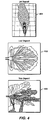
- Jet 401 and leaf 402 deposits are composed of a single body while tree deposits 403 consist of composite sedimentary bodies and channels. Due to their simple body shapes and composition, jet 401 and leaf 402 deposits are chosen to illustrate this invention. However, various embodiments of the invention can be applied to other deposits as well. Additionally, various embodiments may be applied to systems other than sedimentary deposits.
- the numerical model outputs two classes of variables: flow variables and deposit variables.
- Flow variables include turbidity current thickness, velocity, concentration, and grain sizes
- deposit variables include deposit layer top/base, grain sizes, porosity, and permeability. Both flow and deposit variables are functions of time and space. They are difficult to use for sensitivity analysis. Instead, the present example focuses on those model responses that have direct implications to reservoir modeling.
- the main objective for the numerical model is to simulate a sedimentary deposit that represents a particular reservoir of interest. There are several ways to measure the deposit that is being simulated. For jet and leaf deposits 401, and 402, in this example, the model responses of interest are shape and internal composition of the deposit.
- DAR deposit aspect ratio
- DVF deposit volume fraction
- NTG net-to-gross ratio
- deposit length ( L ) and average thickness ( H ) can be used as model responses as well.
- the foregoing responses can be measured and observed from seismic surveys to provide the global measures for a deposit. They can be used as seismic-derived conditioning data for sedimentary process simulation if they are available.
- Responses that can be measured/observed from well data (cores and logs) are, for example, deposit thickness ( THK ) , net-to-gross ( NTG ), grain size ( GS ), sorting ( ST ), grain size gradient ( GSG ) , and sorting gradient ( STG ) .
- Well data responses provide the local measures of a deposit along well bores in the deposit. They can be used as well-derived conditioning data for sedimentary process simulation if they are available.
- step 202 includes performing Global Sensitivity Analysis (GSA) on the various parameters.
- GSA Global Sensitivity Analysis
- step 202 includes three sub-steps: 2.1 Latin hypercube sampling, 2.2 sedimentary process simulation, and 2.3 sensitivity analysis.
- various embodiments represent the space with a finite number of representative points.
- sampling procedures e.g., Monte Carlo sampling, importance sampling, orthogonal sampling, and Latin hypercube sampling (LHS) etc., in which LHS is the most efficient and effective (Helton and Davis, 2003) for this example.
- McKay et al. (1979) introduced LHS to overcome the slow convergence of the Monte Carlo sampling method.
- Use of LHS accelerates the convergence of the sampling processes, and as a result, reduces the number of points needed to represent the input parameter space.
- the basic idea of LHS is to divide the CDF (cumulative distribution function) interval [0, 1] into equal-spaced subintervals and then to use Monte Carlo sampling in each subinterval. Because random sampling is only in smaller intervals rather than in the entire interval, LHS substantially guarantees that every segment of the entire domain of a given input variable can be sampled with equal probability.
- the use of LHS can reduce unwanted or repeated sampling points.
- a correlation structure or correlation matrix is used to generate meaningful results for sensitivity analysis.
- Iman and Conover (1982) proposed a method for controlling the correlation structure in LHS based on rank correlation and this method can be used in one or more embodiments.
- the correlation structure within the input parameters is preserved in the sample points.
- Table 2 shows an example correlation matrix between input parameters.
- turbidity current can be as small as a couple of kilometers (e.g., about nine km for the Rhone delta of Lake Geneva (Lambert and Giovanoli, 1988)) and as large as a thousand kilometers (e.g., about one thousand km for the Grand Banks (Johnson, 1964)). This example simulation domain design is consistent with these observations.
- a fixed number of uniformly rectangular cells (100 ⁇ 150) are chosen for all simulation runs.
- the inlet (orifice) is placed at the center of the first row of the simulation grid, i.e., cell (75, 1).
- Length ( dy ) of each cell is set to be twice of the width ( dx ) of the cell.
- the turbidity current at the inlet (orifice) flows toward the y direction into the simulation domain.
- the width ( dx ) of the simulation cell for a simulation run is equal to the width of the inlet (orifice) calculated using the given inlet aspect ratio. Because the inlet aspect ratios for the simulation runs are different, the sizes of the simulation cells for different simulation runs are also different.
- this example uses an output scheme by which simulation runs are reported at the same dimensionless times.
- a fixed value of dimensionless time interval i.e., one thousand
- the reporting time index can be used as a dimensionless time to estimate dimensionless avulsion time ( DAT ) .
- Simulation runs for the sample points generated in the LHS operation can be conducted using either a batch process on a computer or a parallel process on a cluster of computers.
- Post processing is then used to calculate the model responses (e.g., NTG, DAR, and DVF ) from the simulation results as a function of time after the simulation runs are finished.
- This example focuses on jet/leaf deposits, so that only response values at avulsion time are needed for sensitivity analysis and conditioning.
- Table 3 shows an example table for ten input parameters and four responses in columns and sample points in rows. The discussion now transitions to studying the sensitivity relationships between the input parameters and the responses.
- the basic assumption for the sensitivity analysis used in this example is that the relationships between the model responses and input parameters are linear. If a linear relationship between an input and a response does not exist, at least one transformation may be used to create a linear relationship. There are two types of nonlinearities between an input parameter and a response: monotonic and non-monotonic. Various embodiments use a monotone transformation method to transform a non-monotonic relationship to a monotonic relationship. The second transformation method that can be used is the rank transformation method that transforms a monotonic nonlinear relationship to a normalized linear relationship. When relationships between responses and input parameters are monotonic, only rank transformation is typically needed because a monotonic relationship already exists. Otherwise, both the monotonic and rank transformations should be used.
- Helton and Davis (2003) proposed a method to handle non-monotonic relationships between responses and input parameters and the method may be used in various embodiments.
- Their method first divides the values of an input parameter into a sequence of mutually exclusive and exhaustive subintervals containing equal numbers of sampled values, and then three statistical tests ( F -test, ⁇ 2 -test, and Kruskal-Wallis test) are performed.
- the three tests for non-monotonic relationships can identify input parameters that might otherwise be missed using standard regression-based sensitivity analysis.
- the rank transformation is an effective transformation that transforms raw data from nonlinear to linear.
- the analysis with rank-transformed data is typically more effective than the analysis with raw data (Iman and Conover 1979, Conover and Iman 1981, Saltelli and Sobol 1995).
- Rank transformation standardizes input/response automatically, but it is generally only appropriate for monotonic relationships.
- Sensitivity analysis is a process that determines the effects of individual input parameters on the individual responses. The effects can be ordered according to the magnitudes of their values to demonstrate the relative importance of each input parameter on a given response and the order can be shown in a tornado chart.
- FIGURE 1 illustrates exemplary sensitive 101, insensitive 103, and oversensitive 102 relationships in an intuitive format.
- y r is a rank transformed response
- s k is the sensitivity coefficient of the k th input parameter to the given response
- x rk is the k th rank transformed input parameter
- N is the number of input parameters
- ⁇ is a random error with zero mean.
- s k is also called SRRC (standard rank transformed regression coefficient). It is a measure of the sensitivity between an input parameter and a response.
- a standard regression method may be used to estimate s k .
- a positive s k means the given response is positively correlated with the k th input parameter, i.e., the response increases as the k th input parameter increases.
- a negative s k means a negative correlation between the given response and the k th input parameter or the response decreases as the k th input parameter increases.
- ) indicates that the k th input parameter is more sensitive to the response while a smaller
- FIGURE 7 An example of the importance of the input parameters is shown in FIGURE 7 as a tornado chart wherein parameters near the top are generally considered to be more important to the particular analysis.
- the p -value of the t- hypostasis test for s k is used to check if s k affects y r .
- a stepwise regression analysis may be used to detect interactions between variables and to protect against over fit.
- FIGURE 8 shows an example cross plot of NTG between simulation and sensitivity model.
- RMV includes two sub-steps: (3.1) multidimensional scaling (MDS) and (3.2) response maps (2D)/volumes (3D).
- MDS provides a useful tool to visualize the input parameter space in a two or three dimensional space. This discussion denotes the relationship for a response in the two-dimensional space a "response map" and in the three-dimensional space a “response volume.”
- MDS has been developed primary in psychology and has been applied successfully in psychology, political science, and marketing in the last several decades (Borg and Groenen, 1997, pp. 1-14). It is almost unknown in engineering and geology. MDS is a statistical technique used to analyze the structure of similarity/dissimilarity data in multidimensional space.
- MDS roles There are four MDS roles (Borg and Groenen, 1997, pp.1-14): (1) as a method that represents similarity/dissimilarity data as distances in a low-dimensional space to make these data accessible to visual inspection and exploration, (2) as a technique that allows testing of structural hypotheses, (3) as a psychological model for exploring psychological structures, and (4) as a data-analytic approach that allows discovery of the dimensions that underlie judgments of similarity/dissimilarity. The first role is quite useful in this example embodiment.
- the MDS described in this example includes a method that represents a set of sampling points obtained in a higher multidimensional parameter space in a lower multidimensional space, usually a two- or three-dimensional space, while maintaining the proximity (e.g., distance) among the sampling points.
- the proximity can be defined as a similarity or dissimilarity. Similarity can be described using, e.g., Pearson correlation coefficient while dissimilarity can be measured using, e.g., Euclidean distance. Therefore, the MDS method used in this example has the ability to preserve the Euclidean distances between the sampling points from the original high-dimensional space to a two- or three-dimensional space.
- MDS models absolute, ratio, interval, and ordinal, which can be used in various embodiments of the invention. This example focuses on the absolute MDS model in which each dissimilarity d ij must match the distance between sample points i and j in the representation space.
- the MDS of this example preserves the distances between sampling points after the number of the dimensions of the multidimensional space has been reduced.
- the measure of the distance changes for sampling points in a lower dimensional space is called stress, a terminology from psychology. Stress measures the error caused by the deduction of spatial dimension. Several formulas can be used to define a stress.
- the first plot is the stress plot that shows the stress (the vertical axis) as a function of the number of dimensions (the horizontal axis).
- FIGURE 9 shows example stress plot 901.
- Another plot is Shepard diagram 902 that is a cross plot between distance d ij (the vertical axis) and dissimilarity D ij (the horizontal axis) for a given dimension.
- FIGURE 9 shows an example Shepard diagram 902 for a stress of 0.064.
- a Shepard plot gives an intuitive picture about the quality of MDS.
- Kruskal's suggestion can be adapted in this example as well.
- the number of dimensions for visualization can be determined based on a given acceptance criteria. For example, if an acceptance criterion is at least a "fair", i.e., stress ⁇ 0.1, the case shown in stress plot 901 and FIGURE 9 should have three dimensions to represent an acceptable response map. Borg and Groenen (1997, pp.
- Kruskal's above classification may not work because a need for more systematic insights into how stress depends on the number of points, the dimensionality of the MDS solution, the kind and amount of error in the proximities, and the type of the underlying true configuration.
- One intuitive technique is to look at an "elbow" in a stress curve, which is a point where the decrements in stress begin to be less pronounced. The elbow gives an indication of the dimensionality that should be chosen.
- Kruskal's classification and the "elbow" point concept are used to determine the number of dimensions that should be used.
- the first aspect is creating the sensitivity-based input parameter space.
- the second aspect is calculating similarity/dissimilarity matrix.
- the third aspect is performing MDS analysis.
- the first of the foregoing aspects of MDS is creating a sensitivity-based input parameter space.
- the original input parameter space may be very difficult to visualize because the magnitude of parameter values in each dimension can be very different, for example, slope is on the order of 10 -4 while inlet aspect ratio is on the order of 10 2 .
- the rank transformation can be used to normalize the input parameter space, thereby compensating for different magnitudes of parameter values.
- the sensitivity study has shown that the input parameters do not equally contribute to a given response. Therefore, it is possible to scale the rank transformed input parameters based on their contributions to the given response. Based on Equation 5, the rank transformed input parameters should be scaled by using the absolute value of the sensitivity coefficients.
- the second of the foregoing aspects of MDS is calculating the similarity/dissimilarity matrix, i.e., the Euclidean distance matrix.
- the Euclidean distance between any two sampling points in the sensitivity-based input parameter space is calculated using Equation 6.
- MDS is performing MDS analysis.
- a tool that can be used in some embodiments is XLSTATTM, a commercial software package developed by Addinsoft.
- MDS is selected with the dissimilarity matrix, absolute model, and dimensions from one to six to construct the stress plot (e.g., 901 of FIGURE 9 ) from which the number of dimensions needed can be determined.
- a Shepard diagram e.g., 902 of FIGURE 9
- the next step is to construct response maps/volumes in part 3.2 of step 203.
- FIGURE 10 shows an example 2D response map 1001 in which the color represents NTG that changes from a large value in red color to a small value in blue color.
- Response map 1001 is in black and white but is adapted from a color map with a continual progression of color change from red to blue.
- mapping 1001 For ease of illustration, areas are indicated in map 1001 where one or more colors dominate.
- the sampling points are represented with their sample point identifications (this is a seventy-five sample-point set with the sample identification changing from one to seventy-five).
- From response maps the relationship between the given response and its input parameters can be visualized by a human user who is used to one-, two-, and three-dimensional concepts. Because 2D is typically easier to visualize than three-dimensional (3D), the embodiments use 2D.
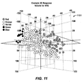
- FIGURE 11 shows example 3D response volume 1101 in which the response is NTG and its value increases as the color (size) of a sampling point changes from blue (small) to red (large).
- Volume 1101 is in black and white but is adapted from a color volume in which the spheres include a color. For ease of illustration, areas of volume 1101 wherein one or more colors dominate are noted.
- step 204 sedimentary process simulations are conditioned to seismic data.
- the goal of this step is to find an intermediate solution space (i.e., seismic-conditioned ensemble) where model responses match the measured/observed seismic data.
- FIGURE 12a shows the conditioning procedures for DAR
- FIGURE 12b shows the conditioning procedures for both DAR and H.
- Bars 1201 and 1202 show the ranges of the input parameters while 2D response maps 1210 and 1220 show the parameter space mapped to DAR and H values. Because the vertical and horizontal coordinates of maps 1210 and 1220 are nonlinear functions with the input parameters, the coordinates and their scales cannot be displayed meaningfully. In MDS, the coordinates are usually called dimensions one and two for a 2D map.
- 2D response maps 1210 and 1220 are adapted from color but are in black and white. While not shown herein, the color in DAR maps 1210 gradually change from red to blue from the top right corner to the bottom left corner. In H maps 1220, the color changes from red in the lower right corner to blue in the top left corner.
- the conditioning process starts with the initial ensemble (the unconditioned parameter space represented by bars and initial response maps) that is large enough to encompass the solutions to the given values of responses.
- a subspace of the initial ensemble can be defined using the constraint of the value range of the response.
- the reduced ensemble can be represented on other response maps, e.g., response map 1220 for H.
- the reduced ensemble can also be illustrated using bars 1202 for the input parameters.
- Bars 1201 of FIGURE 12a show that the ranges of the input parameters ( S and ⁇ ) are shrunk to the reduced ensemble after being conditioned to the given values of DAR.
- the reduced ensemble further shrinks to contain the only values of given H on response map 1220 in FIGURE 12b .
- the further reduced ensemble can also be shown on other maps, e.g., response map 1210 illustrated in FIGURE 12b , and bars 1201 and 1202 of the input parameters. Any of bars 1201, 1202 and/or maps 1210, 1220 can be displayed to a user when using one or more embodiments of the present invention. The same process is repeated for all other responses until the constraints of the values of all given responses have been applied.
- the process shows a continuous improvement in which the ensemble shrinks when new response data is added.
- the size of the ensemble can shrink to be very small compared to that of the initial ensemble, but the ensemble does not shrink to a single point unless perfect data and knowledge are available (and they are not in real world systems).
- the reduced ensemble is the seismic-conditioned ensemble (intermediate solution space) shown in FIGURE 2 .
- step 205 steps 201-203 are repeated to prepare for conditioning with one or more setup responses. Before conditioning sedimentary process simulation to wells, steps 201-203 are performed.
- Step 205 includes constructing the new range and distribution function for each input parameter based on the seismic-conditioned ensemble. This is typically straightforward because a range for each input parameter is known after the seismic-conditioned ensemble is generated in previous steps. In this example, the uniform distribution for each input parameter is assumed because the range for each parameter is an interval(s) of the original distribution function and a uniform distribution is the simplest form of distribution functions that can be used to fit the original distribution function in that interval(s).
- New LHS sample points are generated from the seismic-conditioned ensemble and GSA is carried out using the responses defined at each well: deposit total thickness ( THK ), net-to-gross ( NTG ) , grain size ( GS ), sorting ( ST ) , grain size gradient ( GSG ) , and sorting gradient ( STG ) .
- THK, NTG, GS, and ST are all defined for the entire interval of the intersection between a well and a deposit while GSG and STG are the average gradients of local (layer-based) GS and ST in the entire interval, respectively.
- the response maps/volumes for each well are created.
- step 206 sedimentary process simulations are conditioned to well data.
- the last step for exemplary SSM method 200 is to condition the reduced ensemble to well data (responses).
- the conditioning method for well data is similar to the seismic-conditioning method except different responses are used. The former applies the model responses measured at each well location and the latter utilizes the model responses measured for the entire deposit.
- the size of the seismic-conditioned ensemble is expected to be continuously reduced. If the process is successful, the final solution space, i.e. the well- and seismic-conditioned ensemble, is created, and then the entire conditioning process for sedimentary process simulation using SSM is finished.
- test case conditions sedimentary process simulations to seismic data first and then conditions the simulations to well data.
- the test case also shows the use of sensitivity analysis and MDS.
- FIGURE 13 shows a case to demonstrate a method of conditioning sedimentary numerical models to seismic data, according to an embodiment of the invention.
- Thickness map 1301 for the deposit of this case (a jet/leaf deposit) is illustrated, and the model responses that may be estimated from a seismic survey are shown in the table next to map 1301.
- Thickness map 1301 is a black and white illustration adapted from a color illustration where color indicates depth. For ease of illustration, the color has been removed from map 1301 but is indicated in text.
- the thickness of the deposit varies in a range from zero to fifty meters.
- Table 4 summarizes the true input parameters that are used to generate the deposit. These input parameters, called “truth” in the case study, are assumed to be unknown in the conditioning process and are almost always unknown in real world studies. In this case, truth parameters are used to validate the solution from conditioning. Because it is generally impossible to measure the deposit from a seismic survey precisely in reality, uncertainties are always associated with the estimated responses. Table 5 summarizes the uncertainty and range for each response that is applied in the conditioning case study. Notice that the 5% uncertainty assumption for NTG is too low for a complex deposit (tree deposit) because no currently available seismic survey is able to measure NTG with such accuracy. However, for jet/leaf deposits, the 5% uncertainty for NTG is a reasonable assumption.
- FIGURES 14-18 are organized in a uniform way to demonstrate this embodiment of the invention.
- the first feature is the conditioning (measured/observed) data that includes the given response values and their uncertainties ( ⁇ %, percent errors) shown on the upper right corner of each figure.
- the second feature is the parameter space that is illustrated with vertical bars 1410, 1510, 1610, 1710 and 1810.
- the legends for bars 1410, 1510, 1610, 1710, and 1810 can be found on the upper left corner of each figure.
- Vertical bars 1410, 1510, 1610, 1710, and 1810 show the range of each input parameter as a function of conditioning data where the left-most bars in each set represent the entire parameter space (initial ensemble).
- the changes of bars 1410, 1510, 1610, 1710, and 1810 from left to right in each grouping reflect the change of the ensemble due to the constraints of the given responses imposed on the parameter space.
- the third feature is response maps 1420, 1520, 1620, 1720 and 1820.
- Response maps 1420, 1520, 1620, 1720 and 1820 are labeled with their corresponding response names.
- the 2D maps e.g., maps 1420a-d
- maps 1420a-d are the responses that define the entire parameter space (initial ensemble) while the irregular polygons therein represent the reduced ensemble in which the values of response maps match the given responses and uncertainties.
- response maps 1420, 1520, 1620, 1720 and 1820 are adapted from color maps, as with FIGURES 12a and 12b .
- response maps 1420, 1520, 1620, 1720 and 1820 are the same, except that the polygons therein change as conditioning is performed. As more conditioning data is given, the polygons in each map 1420, 1520, 1620, 1720 and 1820 are expected to shrink if the new given conditioning data has an impact on the ensemble (i.e., is sensitive to the input parameters).
- FIGURE 14 shows the reduced ensemble after the parameter space is conditioned to the given DAR (0.8) response and its uncertainty (10%).
- the conditioning process begins by digitizing a polygon on DAR response map 1420a. The values of DAR inside the polygon fall in the given range of DAR. Once the polygon is constructed, it can be displayed on other response maps, e.g., NTG, DVF, H, and L shown in FIGURE 14 . These polygons, the shapes of which can be very different on different response maps, are the representations of the reduced ensemble and serve as an intuitive illustration for human users.
- the reduced ensemble can also be shown in the parameter space as the vertical (right-hand) bars of each small grouping of bars 1410 in FIGURE 14 that represent the reduced range of each parameter with new minimum and maximum.
- the reduced ensemble can be visualized using vertical bars 1410 in the parameter space and the polygons on response maps 1420.
- Both the polygons and vertical bars 1420, 1520, 1620, 1720, and 1820 in FIGURES 14-18 show that conditioning to the given DAR is successful because the size of the ensemble is reduced.
- the input parameters with the largest changes are slope ( S ), inlet aspect ratio ( R L ), mean grain size ( ⁇ ), velocity ( V ), drag coefficient ( c D ), Froude number ( F R ), and depositional porosity ( ⁇ ).
- FIGURE 15 shows that the reduced ensemble continuously shrinks after being conditioned to the given NTG (0.96) and its uncertainty (5%).
- a new polygon that encompasses the given NTG values is digitized inside the existing polygon on NTG response map 1520b to create a new ensemble.
- the new reduced ensemble is then displayed on the other response maps 1520a and 1520c-d and as the new vertical bars in the parameter space.
- Vertical bars 1520 show that conditioning to the given NTG ranges affects the ranges of mean grain size ( ⁇ ), sorting ( ⁇ ), and Froude number ( F r ).
- FIGURE 16 shows that conditioning to DVF causes changes of the polygons on the NTG, H, and L response maps (1620b, 1620d, and 1620e).
- the input parameters that have clear changes are mean grain size ( ⁇ ), sorting ( ⁇ ), drag coefficient ( c D ), and alpha ( ⁇ ).
- the ensemble size drops as new information is added.
- FIGURE 17 shows that the polygons of the new ensemble shown on all of the response maps shrink as the conditioning data for H is used.
- the input parameters with clear changes in their ranges are slope ( S ), drag coefficient ( c D ), Froude number ( F r ), mean grain size ( ⁇ ), and depositional porosity ( ⁇ ).
- FIGURE 18 shows that the size of the reduced ensemble shown as the polygons on all response maps 1820 and the ranges of most input parameters (vertical bars) dramatically drops.
- the input parameters that show a large impact are slope ( S ), inlet aspect ratio ( R L ), drag coefficient ( c D ), velocity ( V ), mean grain size ( ⁇ ), and depositional porosity ( ⁇ ).
- the true input parameters and responses are displayed on vertical bars 1810 and response maps 1820 as points.
- FIGURE 18 shows that truth is inside the polygons and the parameter ranges, which validates the conditioning process.
- Table 6 summarizes the changes of the ranges of the input parameters as a result of the above conditioning process.
- Table 6 summarizes the changes of the ranges of the input parameters as a result of the above conditioning process.
- the ranges of the input parameters in the ensemble that do not converge to a single point indicate that the available conditioning information is not sufficient enough to identify the truth.
- the process demonstrates that an ensemble that includes the truth may be identified. The estimation and understanding of the truth improve as more information is available.
- FIGURE 19 illustrates a graphical comparison of deposit thickness maps between the four samples and the truth.
- the deposit thickness maps of FIGURE 19 are similar to the maps of FIGURE 13 and are adapted to black and white from color. As in FIGURE 13 , the colors generally follow the contour lines.
- Both Table 8 and FIGURE 19 show that the ensemble (intermediate solution space) reproduces the truth reasonably well. In the next section, it is shown that the uncertainty in the solution can be continuously reduced when the sedimentary process simulations are conditioned to well data.
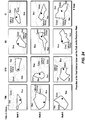
- FIGURE 20 shows the positions of three wells (relative to the truth) that are selected for the conditioning study.
- Well-1 is chosen in the distal area near the orifice (inlet)
- well-2 is located on the levee
- well-3 is selected in the distal area far away from the orifice (inlet).
- Responses at the three wells are deposit thickness ( THK ), net-to-gross ( NTG ), grain size ( GS ), sorting ( ST ), grain size gradient ( GSG ), and sorting gradient ( STG ) .
- THK, NTG, GS, and ST are all defined for the entire interval of the intersection between a well and a deposit while GSG and STG are the gradients of local (layer-based) GS and ST in the entire interval, respectively.
- the first response, THK is the thickness of the deposit at a given well location. It is calculated as the difference between the top value (elevation) of the top layer of the deposit and the base value of the bottom layer of the deposit.
- NTG is calculated using sand volume ( V D -V S ) divided by V D (deposit volume).
- ⁇ k is the fraction of sand for layer k
- C kl is the concentration of grain l at layer k whose size D / is larger than a shale grain size threshold D t
- n s is the number of grain sizes.
- the shale grain size threshold D t used is equal to 60 ⁇ m, or 0.06 mm.
- GS and ST are relatively simple.
- the grain size concentrations of the layers in a given well are combined according to their volumes into a single grain size distribution for the entire well.
- GS and ST are computed directly using the mean and standard deviation of the single grain size distribution function, respectively.
- GSG describes a fining or coarsening direction in a well. If GSG is positive, the grain size distribution in the well is coarsening upward. Otherwise, the grain size distribution in the well is fining upward.
- this example embodiment calculates the mean grain size for each layer in the well and assigns it to the center of the layer. Then, a table of layer-mean grain size and layer center elevation can be constructed. A linear regression method is used to calculate the slope of layer-mean grain size as a function of layer center elevation. The calculated slope is the expected GSG.
- Calculation of STG is similar to the calculation of GSG, except that layer sorting is used as the dependent variable in regression, instead of using layer-mean grain size.
- Table 9 summarizes the "measured/observed” values of the six responses in well-1, well-2, and well-3 from the "truth" model shown in FIGURES 13 and 20 .
- TABLE 9 Response Symbol Unit Value (Well-1) Value (Well-2 Value (Well-3) Deposit thickness THK m 2.24 18.17 2.6 Net-to-gross NTG 0.922 0.996 0.98 Mean grain size GS mm 0.112 0.393 0.143 Sorting ST phi 0.56 0.832 0.474 Grain size gradient GSG mm/m 0.1089 -0.0091 -0.1089 Sorting gradient STG phi/m 0.00399 0.00164 -0.02254
- the seismic-conditioned ensemble is used to create the ranges and distributions for the new input parameter space.
- One-hundred fifty LHS sample points are generated from the input parameter, one-hundred fifty simulation runs are carried out, and sensitivity analysis is conducted in the second step. Using the sensitivity results, MDS is performed and response maps are created.
- the example embodiment includes conditioning the seismic-conditioned ensemble to the response data collected from wells 1, 2, and 3. After this conditioning, the seismic- and well-conditioned ensemble (final solution space) is created.
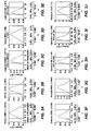
- FIGURE 21 shows cross plots between simulation (vertical axis) and sensitivity model (Equation 5, horizontal axis) for the responses at the three wells.
- a good correlation indicates a strong relationship between a response and the input parameters.
- a R 2 equal to 0.9 means that 90% of the variability of the response can be explained by the variability of the input parameters using the sensitivity model.
- R 2 is small, the unexplained portion of the variability of the response is large and thus the chance to estimate the true input parameters from the response is small. Therefore, studying the value of R 2 can help to eliminate the responses that have a very small R 2 (e.g., ⁇ 0.5) from the candidates for conditioning.
- sorting gradient STG should be removed from conditioning because its R 2 s for the three conditioning wells are all smaller than 0.5.
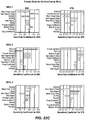
- FIGURE 22 shows tornado charts for responses at the three wells.
- the tornado charts of FIGURE 22 illustrate the ranking of importance of the input parameters on each individual response and can be used to determine or eliminate insensitive parameters.
- the three most important input parameters (in this particular study) for all of the responses are sorting ( ⁇ ), velocity ( V ), and mean grain size ( ⁇ ).
- sorting ⁇
- V velocity
- ⁇ mean grain size
- conditioning to the three wells may reduce the uncertainty of the three input parameters (sorting, velocity, and mean grain size) because they have the largest impact on the responses.
- the sorting in the deposit (ST) is mainly controlled by the sorting ( ⁇ ) in the flow at the orifice (inlet). Therefore, the chance of success to estimate the sorting of grain sizes in the flow at the inlet by studying the sorting of grain sizes in the deposit at a well is large.
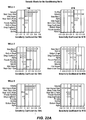
- FIGURE 23 The table shown at the upper right corner of FIGURE 23 gives the conditioning data for wells 1, 2, and 3.
- the values of uncertainty ( ⁇ %) are given by considering the correlations between responses and the input parameters shown in FIGURE 21 .
- the seismic-conditioned ensemble is expected to continuously reduce when the numerical model is conditioned to well data.
- FIGURE 23 shows the further reduced solution spaces for the three wells. From FIGURE 23 , it is apparent well 3 has the smallest overall contribution to reducing the size of the solution space, compared to the contributions of wells 1 and 2. Therefore, well 3 may be not an ideal location for conditioning.
- FIGURE 23 further implies that as the distance of a well from the orifice (inlet) increases, the chance of success to identify the input parameters decreases.
- FIGURE 23 also shows that the input parameters that have the overall largest changes in their ranges are sorting ( ⁇ ), velocity ( V ), and mean grain size ( ⁇ ), which is consistent with the sensitivity analysis results shown in FIGURE 22 . Therefore, the largest contribution of conditioning to well data is on refining the estimation of the sorting ( ⁇ ), velocity ( V ), and mean grain size ( ⁇ ) in the flow at the orifice.
- the parameters with the overall smallest changes in their ranges are Slope ( S ) and Alpha ( ⁇ ), which may indicate that the chance of success to identify the values of S and ⁇ from well data is small.
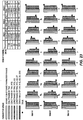
- FIGURE 24 Conditioning the seismic-conditioned parameter space to data from the three wells creates the seismic- and well-conditioned ensemble (final solution space) that is shown as polygons on the response maps in FIGURE 24 .
- the response maps of FIGURE 24 represent the seismic-conditioned parameter space and the values of the responses increase as the color scale changes from blue to red.
- FIGURE 24 is adapted from a color illustration, and the color is not reproduced herein.
- FIGURE 24 represents an intuitive way to illustrate conditioning and uncertainty to a user after a second round of response data is used for conditioning.
- the dots represent the truth in the seismic-conditioned parameter space for validation purposes in this example.
- Table 10 shows the comparison of the ranges of the input parameters changing from the original unconditioned ensemble to the seismic-conditioned ensemble to the seismic- and well-conditioned ensemble.
- the ensembles continuously shrink and the estimation of the input parameters is getting more accurate as more conditioning data is added in.
- FIGURE 25 shows the continuous improvement process using the input grain size distribution function as an example.
- FIGURE 25 shows that the size of the unconditioned ensemble is very large. After the original ensemble is conditioned to seismic data, the size of the seismic-conditioned ensemble decreases and converges toward the truth. The size of the seismic- and well- conditioned ensemble further drops as it is conditioned to well data.
- FIGURE 25 clearly shows a converging process toward the truth as new response data is added.
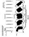
- FIGURE 26 shows a comparison of the grain size distributions in the deposit at different well locations and the estimated input grain size distribution function at the inlet.
- the figure shows that the distribution functions are very different in different locations in the deposit.
- Well 2 shows the coarsest grains with the poorest sorting
- well 3 illustrates the finest grains with the best sorting
- well 1 shows an intermediate sorting.
- the estimated input grain size distribution function in the flow is different from any of the distribution functions in the deposit at the three well locations. From a material balance point of view, the input grain size distribution is the sum of the distributions of the deposit at all locations. If there is an appreciable number of wells and data from those wells, the input grain size distribution for the numerical model can be calculated by summing up the grain size distribution functions measured at the various well locations.
- FIGURE 27 is an illustration of exemplary system 2700 adapted according to the disclosure.
- System 2700 includes a computer or computers with associated hardware and software to perform the functions described above.
- Functional units 2701-2707 can include hardware, software, and any combination thereof. Further, examples of the system are not limited to any particular architecture. For example, while functional units 2701-2707 are shown as separate units, various ones of functional units 2701-2707 may be combined with other ones of functional units 2701-2707. In fact, the functionality shown in FIGURE 2 may be distributed amongst a plurality of computers.
- System 2700 includes functional unit 2701, which creates the initial parameter space.
- Parameter spaces can be set automatically, by input from a user, or a combination of user input and automation.
- Functional unit 2702 provides sampling, such as LHS or any other suitable sampling.
- Functional unit 2703 provides process simulations, such as sedimentary process simulations.
- Functional unit 2704 performs sensitivity analysis.
- Functional unit 2705 creates 2D maps and 3D volumes from the parameter spaces. While the examples herein focus on 2D and 3D visualizations, higher-dimensional visualizations may be used as well. The number of dimensions for most conditioning problems is much larger than ten, such that a substantial reduction in the number of dimensions (even if the end visualization has more than three dimensions) can be quite useful to a human user.
- Functional unit 2706 performs conditioning.
- Functional unit 2706 conditions the parameter space using more than one set of responses.
- functional unit 2706 performs conditioning with respect to a set of responses that are more suitable for a low-density parameter space.
- functional unit 2706 sends the reduced parameter space back to one or more of functional units 2701-2705 to repeat sampling and sensitivity analysis in anticipation of conditioning with respect to a second set of responses. Then, conditioning is performed on the second set of responses that are more suitable for a high-density parameter space, thereby reducing the parameter space even further.
- System 2700 is operable to condition the parameter space using more than two sets of responses.
- Functional unit 2707 includes user input/output hardware and software.
- the user receives output from each functional unit 2701-2706, thereby allowing the user to review the data in a very intuitive form. Additionally, the user can control any of functional units 2701-2706 by inputting information (e.g., by redefining a parameter space, taking action based on results of sensitivity analysis, etc.).
- embodiments of the invention may be adapted for use in any area of science and engineering where an inverse solution of a dynamic system is useful.
- examples that relate to the earth sciences are, but not limited to, conditioning sedimentary process simulation, 4D seismic and hydrocarbon production history matching, seismic inversion, and hydrological model calibration, geophysical surveys, ecosystems, and atmospheric systems.
- various embodiments include one or more advantages over prior art solutions. For example, narrowing a group of parameter values to a range, rather than a single point, tends to give results to a human user that are intuitive in their illustration of uncertainty. Also, narrowing the parameter space to a range eliminates the possibility of becoming "stuck" at a local minimum, which addresses a drawback of prior art optimization approaches.
- various embodiments of the invention address all three issues of the ill-posedness problem. For instance, a user is visually apprised when there is no solution within a parameter space because one or more polygons do not overlap during conditioning. Further, non-smoothness is illustrated to a user during sensitivity analysis, and smoothness issues can be dealt with by the use accordingly. Additionally, various embodiments of the invention provide an intuitive tool to study non-unique solutions as values within a final ensemble in the context of uncertainty.
- the MDS techniques of various embodiments provide a user with a way to visualize the parameter space, even high-dimensional parameter spaces. The user can then more easily understand the parameter space, and can also more easily understand narrowing of the parameter space due to conditioning.
- various elements of embodiments of the present invention are in essence the software code defining the operations of such various elements.
- the executable instructions or software code may be obtained from a tangible readable medium (e.g., a hard drive media, optical media, EPROM, EEPROM, tape media, cartridge media, flash memory, ROM, memory stick, and/or the like).
- readable media can include any medium that can store information.
- FIGURE 28 illustrates an example computer system 2800 adapted according the present disclosure. That is, computer system 2800 comprises an example system on which embodiments of the present invention may be implemented (such as a computer used to enter response data, enter parameter ranges and/or construct an input parameter space, to perform sensitivity analysis, perform MDS and construct response maps/volumes in two or three dimensions, perform conditioning, and the like).
- Central processing unit (CPU) 2801 is coupled to system bus 2802.
- CPU 2801 may be any general purpose CPU, as long as CPU 2801 supports the operations as described herein.
- CPU 2801 may execute the various logical instructions according to the present disclosure. For example, CPU 2801 may execute machine-level instructions according to the exemplary operational flows described above in conjunction with FIGURE 2 .
- Computer system 2800 also preferably includes random access memory (RAM) 2803, which may be SRAM, DRAM, SDRAM, or the like.
- Computer system 2800 preferably includes read-only memory (ROM) 2804 which may be PROM, EPROM, EEPROM, or the like.
- RAM 2803 and ROM 2804 hold user and system data and programs, as is well known in the art.
- Computer system 2800 also preferably includes input/output (I/O) adapter 2805, communications adapter 2811, user interface adapter 2808, and display adapter 2809.
- I/O adapter 2805, user interface adapter 2808, and/or communications adapter 2811 may, in certain examples, enable a user to interact with computer system 2800 to input information, such as response data.
- a user may also interact with system 2800 to modify a parameter space, to modify maps/volumes, to create simulations or analysis data from models, and/or the like.
- I/O adapter 2805 preferably connects to storage device(s) 2806, such as one or more of hard drive, compact disc (CD) drive, floppy disk drive, tape drive, etc. to computer system 2800.
- the storage devices may be utilized when RAM 2803 is insufficient for the memory requirements associated with storing data.
- Communications adapter 2811 is preferably adapted to couple computer system 2800 to network 2812 (e.g., a Local Area Network, a Wide Area Network, the Internet, and/or the like).
- User interface adapter 2808 couples user input devices, such as keyboard 2813, pointing device 2807, and microphone 2814 and/or output devices, such as speaker(s) 2815 to computer system 2800.
- Display adapter 2809 is driven by CPU 2801 to control the display on display device 2810 to, for example, display the user interface (which may show one or more displays such as the maps, tables, and graphs of FIGURES 3 and 7-26 ) of the present disclosure.
- the present disclosure is not limited to the architecture of system 2800.
- any suitable processor-based device may be utilized, including without limitation personal computers, laptop computers, handheld computing devices, computer workstations, and multi-processor servers.
- examples of the present disclosure may be implemented on application specific integrated circuits (ASICs) or very large scale integrated (VLSI) circuits.
- ASICs application specific integrated circuits
- VLSI very large scale integrated circuits
Landscapes
- Engineering & Computer Science (AREA)
- Physics & Mathematics (AREA)
- General Physics & Mathematics (AREA)
- Theoretical Computer Science (AREA)
- Geometry (AREA)
- Software Systems (AREA)
- General Engineering & Computer Science (AREA)
- Evolutionary Computation (AREA)
- Remote Sensing (AREA)
- Computer Hardware Design (AREA)
- Computer Graphics (AREA)
- Life Sciences & Earth Sciences (AREA)
- General Life Sciences & Earth Sciences (AREA)
- Geophysics (AREA)
- Management, Administration, Business Operations System, And Electronic Commerce (AREA)
Claims (10)
- Procédé mis en œuvre par ordinateur pour modéliser des systèmes géologiques dynamiques, ledit procédé comportant les étapes consistant à :construire un espace (201) de paramètres d'entrée pour un modèle de le système géologique, ledit espace de paramètres d'entrée comprenant plus de trois dimensions, ledit modèle étant utilisé pour générer des données de réponse correspondant à des données observées ou expérimentales ;représenter visuellement ledit espace de paramètres d'entrée avec moins de dimensions qu'un nombre de dimensions dudit espace de paramètres d'entrée, pour générer une représentation visuelle dudit espace de paramètres d'entrée, le fait de représenter ledit espace de paramètres d'entrée comportant la représentation d'une pluralité de points dans ledit espace de paramètres dans un espace bidimensionnel tout en maintenant des distances entre points ;restreindre ledit espace de paramètres d'entrée en conditionnant ledit espace de paramètres à l'aide d'au moins un sous-ensemble desdites données de réponse,ledit conditionnement étant caractérisé par :la génération des données de réponse pour au moins un sous-ensemble de ladite pluralité de points dans ladite représentation bidimensionnelle de l'espace de paramètres ;la détermination, dans ladite représentation bidimensionnelle, d'un polygone circonscrivant les points pour lesquels lesdites données de réponse générées se situent dans la limite d'une erreur par rapport aux données observées ou expérimentales, et l'espace de paramètres d'entrée étant visualisé, exploré et examiné pendant le processus de conditionnement ;le procédé comportant en outre :
la mise à jour de ladite représentation dudit espace de paramètres d'entrée pour représenter visuellement ladite restriction dudit espace de paramètres en restituant le polygone sur ledit espace bidimensionnel. - Procédé selon la revendication 1, ledit espace bidimensionnel comprenant un codage en couleurs pour représenter des variations dans des valeurs desdites données de réponse.
- Procédé selon la revendication 1, la construction de l'espace (201) de paramètres d'entrée comportant :
l'échantillonnage de valeurs de paramètres pour générer un nombre discret de points, chacun desdits points correspondant à une valeur d'un paramètre dans ledit espace de paramètres. - Procédé selon la revendication 3, ledit échantillonnage comprenant un échantillonnage par hypercube latin (LHS).
- Procédé selon la revendication 1, l'espace de paramètres comportant une pluralité de modèles et le procédé comportant en outre les étapes consistant à :effectuer une analyse de sensibilité (202) sur les paramètres d'entrée d'un ou plusieurs desdits modèles ; etne pas conditionner les paramètres d'entrée de l'espace de paramètres d'un ou plusieurs desdits modèles qui présentent une sensibilité inférieure à un premier seuil.
- Procédé selon la revendication 5, ladite analyse de sensibilité (202) mesurant un rapport d'une variation dans une sortie d'un modèle donné à une variation dans un paramètre d'entrée d'un modèle donné, un rapport plus élevé indiquant une sensibilité plus élevée.
- Procédé selon la revendication 5 comportant en outre :
l'ajustement des paramètres d'au moins un desdits modèles en réponse au fait qu'une sensibilité des paramètres dudit ou desdits modèles est supérieure à un second seuil. - Procédé selon la revendication 5, la réalisation de l'analyse de sensibilité (202) comportant :
le classement de paramètres d'entrée dudit espace de paramètres d'entrée d'après leurs sensibilités respectives. - Procédé selon la revendication 1, lesdites données de réponse comportant :des données sismiques dudit système géologique ; etdes données de puits dudit système géologique.
- Produit de programme informatique comprenant un support lisible par ordinateur sur lequel est enregistrée une logique de programme informatique servant à réaliser le procédé selon l'une quelconque des revendications précédentes.
Applications Claiming Priority (2)
| Application Number | Priority Date | Filing Date | Title |
|---|---|---|---|
| US12643808P | 2008-05-05 | 2008-05-05 | |
| PCT/US2009/038279 WO2009137181A1 (fr) | 2008-05-05 | 2009-03-25 | Systèmes, procédés et produits de programme informatique pour modéliser des systèmes dynamiques en visualisant un espace de paramètres et en réduisant cet espace de paramètres |
Publications (3)
| Publication Number | Publication Date |
|---|---|
| EP2291790A1 EP2291790A1 (fr) | 2011-03-09 |
| EP2291790A4 EP2291790A4 (fr) | 2017-02-22 |
| EP2291790B1 true EP2291790B1 (fr) | 2020-04-29 |
Family
ID=41264918
Family Applications (1)
| Application Number | Title | Priority Date | Filing Date |
|---|---|---|---|
| EP09743168.8A Active EP2291790B1 (fr) | 2008-05-05 | 2009-03-25 | Modélisation des systèmes dynamiques géologiques en visualisant un espace de paramètres et en réduisant cet espace de paramètres |
Country Status (5)
| Country | Link |
|---|---|
| US (1) | US9372943B2 (fr) |
| EP (1) | EP2291790B1 (fr) |
| AU (1) | AU2009244726B2 (fr) |
| CA (1) | CA2720117C (fr) |
| WO (1) | WO2009137181A1 (fr) |
Families Citing this family (67)
| Publication number | Priority date | Publication date | Assignee | Title |
|---|---|---|---|---|
| US9372943B2 (en) | 2008-05-05 | 2016-06-21 | Exxonmobil Upstream Research Company | Modeling dynamic systems by visualizing and narrowing a parameter space |
| US8374836B2 (en) * | 2008-11-12 | 2013-02-12 | Geoscape Analytics, Inc. | Methods and systems for constructing and using a subterranean geomechanics model spanning local to zonal scale in complex geological environments |
| US8818780B2 (en) | 2008-11-14 | 2014-08-26 | Exxonmobil Upstream Research Company | Forming a model of a subsurface region |
| BRPI0924258A2 (pt) * | 2009-03-05 | 2016-01-26 | Exxonmobil Upstream Res Co | métodos para otimizar e para determinar desempenho de reservatório |
| US8606555B2 (en) * | 2009-10-23 | 2013-12-10 | Chevron U.S.A. Inc. | System and method for modeling a geologic volume of interest |
| US8355872B2 (en) * | 2009-11-19 | 2013-01-15 | Chevron U.S.A. Inc. | System and method for reservoir analysis background |
| CN102870087B (zh) | 2010-04-30 | 2016-11-09 | 埃克森美孚上游研究公司 | 流体有限体积仿真的方法和系统 |
| CA2801386A1 (fr) | 2010-06-15 | 2011-12-22 | Exxonmobil Upstream Research Company | Procede et systeme permettant de stabiliser des procedes de formulation |
| CA2803068C (fr) | 2010-07-29 | 2016-10-11 | Exxonmobil Upstream Research Company | Procede et systeme de modelisation d'un reservoir |
| EP2599031A4 (fr) | 2010-07-29 | 2014-01-08 | Exxonmobil Upstream Res Co | Procédés et systèmes pour une simulation de flux par apprentissage automatique |
| AU2011283190A1 (en) | 2010-07-29 | 2013-02-07 | Exxonmobil Upstream Research Company | Methods and systems for machine-learning based simulation of flow |
| CA2805446C (fr) | 2010-07-29 | 2016-08-16 | Exxonmobil Upstream Research Company | Procedes et systemes de simulation d'ecoulement basee sur un apprentissage machine |
| WO2012039811A1 (fr) | 2010-09-20 | 2012-03-29 | Exxonmobil Upstream Research Company | Formulations souples et adaptatives pour des simulations de gisements complexes |
| AU2011332274B2 (en) | 2010-11-23 | 2017-02-23 | Exxonmobil Upstream Research Company | Variable discretization method for flow simulation on complex geological models |
| WO2012074533A1 (fr) * | 2010-12-03 | 2012-06-07 | James Victory | Appareil et procédé pour synthétiseur de cellule d'alimentation optimisé |
| US8805659B2 (en) * | 2011-02-17 | 2014-08-12 | Chevron U.S.A. Inc. | System and method for uncertainty quantification in reservoir simulation |
| US20120296618A1 (en) * | 2011-05-20 | 2012-11-22 | Baker Hughes Incorporated | Multiscale Geologic Modeling of a Clastic Meander Belt Including Asymmetry Using Multi-Point Statistics |
| US8731891B2 (en) * | 2011-07-28 | 2014-05-20 | Saudi Arabian Oil Company | Cluster 3D petrophysical uncertainty modeling |
| CN103959233B (zh) | 2011-09-15 | 2017-05-17 | 埃克森美孚上游研究公司 | 在执行eos计算的指令受限算法中最优化矩阵和向量运算 |
| US20130110474A1 (en) | 2011-10-26 | 2013-05-02 | Nansen G. Saleri | Determining and considering a premium related to petroleum reserves and production characteristics when valuing petroleum production capital projects |
| US9946986B1 (en) | 2011-10-26 | 2018-04-17 | QRI Group, LLC | Petroleum reservoir operation using geotechnical analysis |
| US9767421B2 (en) * | 2011-10-26 | 2017-09-19 | QRI Group, LLC | Determining and considering petroleum reservoir reserves and production characteristics when valuing petroleum production capital projects |
| US10508520B2 (en) | 2011-10-26 | 2019-12-17 | QRI Group, LLC | Systems and methods for increasing recovery efficiency of petroleum reservoirs |
| US20130110483A1 (en) * | 2011-10-31 | 2013-05-02 | Nikita V. Chugunov | Method for measurement screening under reservoir uncertainty |
| AU2012357785B2 (en) * | 2011-12-20 | 2014-12-04 | Shell Internationale Research Maatschappij B.V. | Automated calibration of a Stratigraphic Forward Modelling (SFM) tool using a Neighborhood Algorithm with explicit escape clauses |
| US9098106B2 (en) * | 2012-08-10 | 2015-08-04 | Comsol Ab | Systems and methods for creating application interfaces for forming and solving problems in a modeling system |
| US10578767B2 (en) | 2012-09-26 | 2020-03-03 | Exxonmobil Upstream Research Company | Conditional process-aided multiple-points statistics modeling |
| EP2901363A4 (fr) | 2012-09-28 | 2016-06-01 | Exxonmobil Upstream Res Co | Suppression des failles dans des modèles géologiques |
| US10650177B2 (en) | 2012-12-20 | 2020-05-12 | Comsol Ab | System and method for creating application interfaces for multiphysics modeling |
| US9297918B2 (en) | 2012-12-28 | 2016-03-29 | General Electric Company | Seismic data analysis |
| US20150003200A1 (en) * | 2013-06-28 | 2015-01-01 | Mike Hall | System and method for determining the position of a sensor in seismic exploration |
| WO2015175216A1 (fr) * | 2014-05-16 | 2015-11-19 | Apache Corporation | Procédés de production de statistiques de production de puits et de réserves |
| US9945703B2 (en) | 2014-05-30 | 2018-04-17 | QRI Group, LLC | Multi-tank material balance model |
| US10319143B2 (en) | 2014-07-30 | 2019-06-11 | Exxonmobil Upstream Research Company | Volumetric grid generation in a domain with heterogeneous material properties |
| US10508532B1 (en) | 2014-08-27 | 2019-12-17 | QRI Group, LLC | Efficient recovery of petroleum from reservoir and optimized well design and operation through well-based production and automated decline curve analysis |
| AU2015339883B2 (en) | 2014-10-31 | 2018-03-29 | Exxonmobil Upstream Research Company | Methods to handle discontinuity in constructing design space for faulted subsurface model using moving least squares |
| AU2015339884B2 (en) | 2014-10-31 | 2018-03-15 | Exxonmobil Upstream Research Company | Handling domain discontinuity in a subsurface grid model with the help of grid optimization techniques |
| WO2016134210A1 (fr) * | 2015-02-20 | 2016-08-25 | Schlumberger Technology Corporation | Analyse et modélisation de scénario de sensibilité microsismique |
| GB2555031A (en) * | 2015-06-17 | 2018-04-18 | Landmark Graphics Corp | Model tuning using boundary flux sector surrogates |
| US10082006B2 (en) | 2015-10-26 | 2018-09-25 | International Business Machines Corporation | Reduced space clustering representatives and its application to long term prediction |
| US11899161B2 (en) | 2015-10-27 | 2024-02-13 | Schlumberger Technology Corporation | Optimization under uncertainty for integrated models |
| CA3024515C (fr) * | 2016-06-02 | 2023-11-28 | Shell Internationale Research Maatschappij B.V. | Procede de traitement d'un ensemble de donnees geospatiales |
| US10458207B1 (en) | 2016-06-09 | 2019-10-29 | QRI Group, LLC | Reduced-physics, data-driven secondary recovery optimization |
| US10794134B2 (en) * | 2016-08-04 | 2020-10-06 | Baker Hughes, A Ge Company, Llc | Estimation of optimum tripping schedules |
| CA3043231C (fr) | 2016-12-23 | 2022-06-14 | Exxonmobil Upstream Research Company | Procede et systeme de simulation de reservoir stable et efficace a l'aide d'indicateurs de stabilite |
| CN106682355B (zh) * | 2017-01-12 | 2018-12-21 | 中国水利水电科学研究院 | 一种基于pso-ga混合算法的水文模型参数率定方法 |
| CA3018334A1 (fr) * | 2017-09-21 | 2019-03-21 | Royal Bank Of Canada | Dispositif et methode d'evaluation de la qualite des visualisations des donnees multidimensionnelles |
| US11126762B2 (en) * | 2018-02-28 | 2021-09-21 | Saudi Arabian Oil Company | Locating new hydrocarbon fields and predicting reservoir performance from hydrocarbon migration |
| US11466554B2 (en) | 2018-03-20 | 2022-10-11 | QRI Group, LLC | Data-driven methods and systems for improving oil and gas drilling and completion processes |
| US11010883B2 (en) | 2018-04-17 | 2021-05-18 | Saudi Arabian Oil Company | Automated analysis of petrographic thin section images using advanced machine learning techniques |
| US11506804B2 (en) * | 2018-05-31 | 2022-11-22 | Saudi Arabian Oil Company | Inverse stratigraphic modeling using a hybrid linear and nonlinear algorithm |
| US11301794B2 (en) | 2018-06-11 | 2022-04-12 | International Business Machines Corporation | Machine for labor optimization for efficient shipping |
| US11301791B2 (en) * | 2018-06-11 | 2022-04-12 | International Business Machines Corporation | Fulfilment machine for optimizing shipping |
| US11506052B1 (en) | 2018-06-26 | 2022-11-22 | QRI Group, LLC | Framework and interface for assessing reservoir management competency |
| WO2020109958A1 (fr) * | 2018-11-30 | 2020-06-04 | Chevron Usa Inc. | Système et procédé d'analyse de données de subsurface |
| US11494854B2 (en) * | 2019-02-07 | 2022-11-08 | Midcontinent Independent System Operator, Inc. | Systems and methods for managing watchlist constraints on an electric power grid |
| CN110046754B (zh) * | 2019-03-29 | 2021-12-10 | 中国海洋石油集团有限公司 | 拉丁超立方抽样油田产液结构优化方法、存储介质及终端 |
| US11604909B2 (en) | 2019-05-28 | 2023-03-14 | Chevron U.S.A. Inc. | System and method for accelerated computation of subsurface representations |
| US11249220B2 (en) | 2019-08-14 | 2022-02-15 | Chevron U.S.A. Inc. | Correlation matrix for simultaneously correlating multiple wells |
| US11187826B2 (en) | 2019-12-06 | 2021-11-30 | Chevron U.S.A. Inc. | Characterization of subsurface regions using moving-window based analysis of unsegmented continuous data |
| US11320566B2 (en) | 2020-01-16 | 2022-05-03 | Chevron U.S.A. Inc. | Multiple well matching within subsurface representation |
| US11263362B2 (en) | 2020-01-16 | 2022-03-01 | Chevron U.S.A. Inc. | Correlation of multiple wells using subsurface representation |
| US11397279B2 (en) * | 2020-03-27 | 2022-07-26 | Chevron U.S.A. Inc. | Comparison of wells using a dissimilarity matrix |
| CN112288169B (zh) * | 2020-10-30 | 2022-03-18 | 成都理工大学 | 二维滑坡动力学参数概率反分析与滑程超越概率评估方法 |
| US11668847B2 (en) | 2021-01-04 | 2023-06-06 | Saudi Arabian Oil Company | Generating synthetic geological formation images based on rock fragment images |
| CN113421336B (zh) * | 2021-08-23 | 2021-11-09 | 武汉幻城经纬科技有限公司 | 动态水域的体绘制方法及装置、存储介质、电子设备 |
| CN113552856B (zh) * | 2021-09-22 | 2021-12-10 | 成都数之联科技有限公司 | 工艺参数根因定位方法和相关装置 |
Family Cites Families (84)
| Publication number | Priority date | Publication date | Assignee | Title |
|---|---|---|---|---|
| US5537320A (en) | 1994-10-31 | 1996-07-16 | Landmark Graphics Corporation | Method and apparatus for identifying fault curves in seismic data |
| US5706194A (en) | 1995-06-01 | 1998-01-06 | Phillips Petroleum Company | Non-unique seismic lithologic inversion for subterranean modeling |
| FR2744224B1 (fr) | 1996-01-26 | 1998-04-17 | Inst Francais Du Petrole | Methode pour simuler le remplissage d'un bassin sedimentaire |
| US5838634A (en) | 1996-04-04 | 1998-11-17 | Exxon Production Research Company | Method of generating 3-D geologic models incorporating geologic and geophysical constraints |
| FR2748516B1 (fr) | 1996-05-07 | 1998-06-26 | Inst Francais Du Petrole | Methode pour realiser un modele cinematique en 2d de bassins geologiques affectes par des failles |
| US6014343A (en) | 1996-10-31 | 2000-01-11 | Geoquest | Automatic non-artificially extended fault surface based horizon modeling system |
| US6128577A (en) | 1996-12-19 | 2000-10-03 | Schlumberger Technology Corporation | Modeling geological structures and properties |
| US5835883A (en) * | 1997-01-31 | 1998-11-10 | Phillips Petroleum Company | Method for determining distribution of reservoir permeability, porosity and pseudo relative permeability |
| US6106561A (en) | 1997-06-23 | 2000-08-22 | Schlumberger Technology Corporation | Simulation gridding method and apparatus including a structured areal gridder adapted for use by a reservoir simulator |
| DE19740565A1 (de) * | 1997-09-15 | 1999-03-18 | Max Planck Gesellschaft | Verfahren zur Erfassung zeitabhängiger Moden dynamischer Systeme |
| US5995906A (en) * | 1997-10-03 | 1999-11-30 | Western Atlas International, Inc. | Method for reconciling data at seismic and well-log scales in 3-D earth modeling |
| FR2776393B1 (fr) | 1998-03-20 | 2001-09-07 | Inst Francais Du Petrole | Methode pour former automatiquement un modele simulant la structure stratigraphique d'une zone souterraine |
| AU2950499A (en) | 1998-05-04 | 1999-11-23 | Schlumberger Evaluation & Production (Uk) Services | Near wellbore modeling method and apparatus |
| US6018498A (en) | 1998-09-02 | 2000-01-25 | Phillips Petroleum Company | Automated seismic fault detection and picking |
| US6246963B1 (en) | 1999-01-29 | 2001-06-12 | Timothy A. Cross | Method for predicting stratigraphy |
| EP1151326B1 (fr) * | 1999-02-12 | 2005-11-02 | Schlumberger Limited | Modelisation de zone souterraine a incertitude reduite |
| US6480790B1 (en) | 1999-10-29 | 2002-11-12 | Exxonmobil Upstream Research Company | Process for constructing three-dimensional geologic models having adjustable geologic interfaces |
| FR2800881B1 (fr) | 1999-11-05 | 2001-11-30 | Inst Francais Du Petrole | Methode pour realiser en 3d un modele cinematique de deformation d'un bassin sedimentaire |
| US6374185B1 (en) | 2000-02-18 | 2002-04-16 | Rdsp I, L.P. | Method for generating an estimate of lithological characteristics of a region of the earth's subsurface |
| US6980940B1 (en) | 2000-02-22 | 2005-12-27 | Schlumberger Technology Corp. | Intergrated reservoir optimization |
| US6370491B1 (en) | 2000-04-04 | 2002-04-09 | Conoco, Inc. | Method of modeling of faulting and fracturing in the earth |
| US7432935B2 (en) * | 2002-11-19 | 2008-10-07 | Mental Images Gmbh | Image synthesis methods and systems for generating sample points in a graphics scene |
| WO2002047011A1 (fr) * | 2000-12-08 | 2002-06-13 | Ortoleva Peter J | Procede de modelisation de domaines multidimensionnels faisant appel a la theorie de l'information pour resoudre les lacunes dans des donnees et dans des theories |
| US8041541B2 (en) | 2001-05-24 | 2011-10-18 | Test Advantage, Inc. | Methods and apparatus for data analysis |
| WO2002099464A1 (fr) | 2001-06-06 | 2002-12-12 | Schlumberger Canada Limited | Systeme automatise pour modelage d'horizons failles a valeur multiple |
| US6541975B2 (en) * | 2001-08-23 | 2003-04-01 | Kjt Enterprises, Inc. | Integrated borehole system for reservoir detection and monitoring |
| US6754558B2 (en) | 2001-08-28 | 2004-06-22 | Vending Management Services Ltd. | Efficient collection of information from vending machines |
| US7248259B2 (en) | 2001-12-12 | 2007-07-24 | Technoguide As | Three dimensional geological model construction |
| US7606691B2 (en) | 2001-12-13 | 2009-10-20 | Exxonmobil Upstream Research Company | Method for locally controlling spatial continuity in geologic models |
| US7069149B2 (en) | 2001-12-14 | 2006-06-27 | Chevron U.S.A. Inc. | Process for interpreting faults from a fault-enhanced 3-dimensional seismic attribute volume |
| US20030182093A1 (en) | 2002-03-25 | 2003-09-25 | Jones Thomas A. | Controlling azimuthally varying continuity in geologic models |
| US7523024B2 (en) | 2002-05-17 | 2009-04-21 | Schlumberger Technology Corporation | Modeling geologic objects in faulted formations |
| US20060122780A1 (en) | 2002-11-09 | 2006-06-08 | Geoenergy, Inc | Method and apparatus for seismic feature extraction |
| US7379854B2 (en) | 2002-12-19 | 2008-05-27 | Exxonmobil Upstream Research Company | Method of conditioning a random field to have directionally varying anisotropic continuity |
| FR2849211B1 (fr) * | 2002-12-20 | 2005-03-11 | Inst Francais Du Petrole | Methode de modelisation pour constituer un modele simulant le remplissage multilithologique d'un bassin sedimentaire |
| US7844430B2 (en) | 2004-01-30 | 2010-11-30 | Exxonmobil Upstream Research Co. | Reservoir model building methods |
| US7596481B2 (en) | 2004-03-16 | 2009-09-29 | M-I L.L.C. | Three-dimensional wellbore analysis and visualization |
| EP1751585B1 (fr) | 2004-06-02 | 2009-11-18 | Paradigm France | Procede de construction d'une partition cellulaire tridimensionnelle d'un domaine geologique |
| US20060047429A1 (en) | 2004-08-24 | 2006-03-02 | Adams Steven L | Method of estimating geological formation depths by converting interpreted seismic horizons from the time domain to the depth domain |
| US8117019B2 (en) | 2004-09-10 | 2012-02-14 | Exxonmobil Upstream Research Company | Method for evaluating sedimentary basin properties by numerical modeling of sedimentation processes |
| EA010285B1 (ru) | 2004-09-10 | 2008-08-29 | Эксонмобил Апстрим Рисерч Компани | Способ построения геологических моделей подземных осадочных объёмов |
| DE602004015297D1 (de) | 2004-10-26 | 2008-09-04 | Total Sa | Verfahren und Computerprogramm zur Fehleroberflächenkonstruktion |
| EP1707993B1 (fr) | 2005-03-29 | 2009-08-19 | Total S.A. | Procédé et programme de recherche de discontinuites géologiques |
| US7480205B2 (en) | 2005-04-20 | 2009-01-20 | Landmark Graphics Corporation | 3D fast fault restoration |
| FR2890453B1 (fr) | 2005-09-05 | 2007-10-19 | Inst Francais Du Petrole | Methode pour mettre a jour un modele geologique de reservoir a l'aide de donnees dynamiques |
| WO2007089829A2 (fr) * | 2006-01-31 | 2007-08-09 | Landmark Graphics Corporation | Procédés, systèmes, et supports lisibles par ordinateur pour la mise à jour rapide de modèles de production de champs de pétrole et de gaz à l'aide de simulateurs physiques et mandataires |
| US9646415B2 (en) * | 2006-05-16 | 2017-05-09 | Underground Imaging Technologies, Inc. | System and method for visualizing multiple-sensor subsurface imaging data |
| US7756694B2 (en) | 2006-05-31 | 2010-07-13 | Schlumberger Technology Corporation | Method for interactive automation of fault modeling including a method for intelligently sensing fault-fault relationships |
| US7254091B1 (en) | 2006-06-08 | 2007-08-07 | Bhp Billiton Innovation Pty Ltd. | Method for estimating and/or reducing uncertainty in reservoir models of potential petroleum reservoirs |
| EP2038810A4 (fr) | 2006-07-07 | 2018-05-09 | Exxonmobil Upstream Research Company | Interpolation de modèles de réservoir par réutilisation de solutions de débit issus de modèles géologiques |
| US7983885B2 (en) * | 2006-12-29 | 2011-07-19 | Terratek, Inc. | Method and apparatus for multi-dimensional data analysis to identify rock heterogeneity |
| JP4802279B2 (ja) | 2007-02-02 | 2011-10-26 | インターデイジタル テクノロジー コーポレーション | 拡張Cell_FACH状態でのセル更新のための方法および装置 |
| US7706981B2 (en) | 2007-02-08 | 2010-04-27 | Chevron U.S.A. Inc. | Method for generating reservoir models utilizing synthetic stratigraphic columns |
| RU2444788C2 (ru) | 2007-06-01 | 2012-03-10 | Эксонмобил Апстрим Рисерч Компани | Создание ограниченной сетки вороного на плоскости |
| US7986319B2 (en) | 2007-08-01 | 2011-07-26 | Austin Gemodeling, Inc. | Method and system for dynamic, three-dimensional geological interpretation and modeling |
| US8577660B2 (en) | 2008-01-23 | 2013-11-05 | Schlumberger Technology Corporation | Three-dimensional mechanical earth modeling |
| US9223041B2 (en) | 2008-01-23 | 2015-12-29 | Schlubmerger Technology Corporation | Three-dimensional mechanical earth modeling |
| US7933750B2 (en) | 2008-04-02 | 2011-04-26 | Schlumberger Technology Corp | Method for defining regions in reservoir simulation |
| CA2721008A1 (fr) | 2008-04-11 | 2009-10-15 | Terraspark Geosciences, Llc | Visualisation de caracteristiques geologiques a l'aide de representations de donnees leur appartenant |
| US9372943B2 (en) | 2008-05-05 | 2016-06-21 | Exxonmobil Upstream Research Company | Modeling dynamic systems by visualizing and narrowing a parameter space |
| US8355898B2 (en) | 2008-06-17 | 2013-01-15 | Chevron U.S.A. Inc. | System and method for modeling flow events responsible for the formation of a geological reservoir |
| US8447522B2 (en) | 2008-07-03 | 2013-05-21 | Baker Hughes Incorporated | Method for estimating the probability of collision between wells |
| BRPI0914102A2 (pt) | 2008-07-03 | 2015-10-20 | Chevron Usa Inc | método de volume finito de multiescalas e sistemas para uso simular um modelo geológico de escala fina de um reservatório de subsuperfície |
| US8255195B2 (en) | 2008-09-18 | 2012-08-28 | Geoscape Analytics, Inc | N-phasic element method for calculating a fully coupled response of multiphase compositional fluid flow and a system for uncertainty estimation |
| US10590762B2 (en) | 2008-09-18 | 2020-03-17 | Geoscale, Inc. | N-phasic finite element method for calculating a fully coupled response of multiphase compositional fluid flow and a system for uncertainty estimation of the calculated reservoir response |
| CA2737724A1 (fr) * | 2008-09-19 | 2010-03-25 | The University Of Sydney | Procede et systeme de modelisation de donnees |
| US8374836B2 (en) | 2008-11-12 | 2013-02-12 | Geoscape Analytics, Inc. | Methods and systems for constructing and using a subterranean geomechanics model spanning local to zonal scale in complex geological environments |
| US8818780B2 (en) | 2008-11-14 | 2014-08-26 | Exxonmobil Upstream Research Company | Forming a model of a subsurface region |
| CA2753544A1 (fr) | 2009-03-27 | 2010-09-30 | Exxonmobil Upstream Research Company | Caracterisation de la qualite d'un reservoir au moyen d'equations d'heterogeneite avec des parametres spatialement variables |
| FR2948215B1 (fr) | 2009-07-16 | 2011-06-24 | Inst Francais Du Petrole | Methode pour generer un maillage hexa-dominant d'un milieu souterrain faille |
| US8655632B2 (en) | 2009-09-03 | 2014-02-18 | Schlumberger Technology Corporation | Gridless geological modeling |
| WO2011037580A1 (fr) * | 2009-09-25 | 2011-03-31 | Landmark Graphics Corporation | Systèmes et procédés pour l'estimation quantitative de l'incertitude d'une prévision de production |
| US8855987B2 (en) * | 2009-10-23 | 2014-10-07 | Exxonmobil Upstream Research Company | Method for optimization with gradient information |
| PL400383A1 (pl) | 2009-12-15 | 2013-01-21 | Schlumberger Technology B.V. | Sposób modelowania basenu zbiornikowego |
| EP2534606B1 (fr) * | 2010-02-12 | 2019-02-27 | Exxonmobil Upstream Research Company | Procédé et programme d'ordinateur de création de modèles de simulation mis en correspondance avec un historique et procédé correspondant de production d'hydrocarbures d'un champ d'yhdrocarbures |
| US8452580B2 (en) | 2010-02-26 | 2013-05-28 | Chevron U.S.A. Inc. | Method and system for using multiple-point statistics simulation to model reservoir property trends |
| US8515720B2 (en) | 2010-04-06 | 2013-08-20 | Schlumberger Technology Corporation | Determine field fractures using geomechanical forward modeling |
| US8731887B2 (en) | 2010-04-12 | 2014-05-20 | Exxonmobile Upstream Research Company | System and method for obtaining a model of data describing a physical structure |
| US20110310101A1 (en) | 2010-06-22 | 2011-12-22 | Schlumberger Technology Corporation | Pillar grid conversion |
| FR2962835B1 (fr) | 2010-07-16 | 2013-07-12 | IFP Energies Nouvelles | Methode pour generer un maillage hexa-dominant d'un bassin geometriquement complexe |
| US8515678B2 (en) | 2010-07-29 | 2013-08-20 | Schlumberger Technology Corporation | Chrono-stratigraphic and tectono-stratigraphic interpretation on seismic volumes |
| AU2011339017B2 (en) | 2010-12-08 | 2016-09-08 | Exxonmobil Upstream Research Company | Constructing geologic models from geologic concepts |
| US8843353B2 (en) | 2011-08-25 | 2014-09-23 | Chevron U.S.A. Inc. | Hybrid deterministic-geostatistical earth model |
| US10977396B2 (en) * | 2012-01-13 | 2021-04-13 | Schlumberger Technology Corporation | Determining an elastic model for a geologic region |
-
2009
- 2009-03-25 US US12/920,266 patent/US9372943B2/en active Active
- 2009-03-25 EP EP09743168.8A patent/EP2291790B1/fr active Active
- 2009-03-25 CA CA2720117A patent/CA2720117C/fr active Active
- 2009-03-25 WO PCT/US2009/038279 patent/WO2009137181A1/fr active Application Filing
- 2009-03-25 AU AU2009244726A patent/AU2009244726B2/en not_active Ceased
Non-Patent Citations (1)
| Title |
|---|
| None * |
Also Published As
| Publication number | Publication date |
|---|---|
| US9372943B2 (en) | 2016-06-21 |
| AU2009244726B2 (en) | 2014-04-24 |
| EP2291790A1 (fr) | 2011-03-09 |
| CA2720117C (fr) | 2017-11-28 |
| US20110054869A1 (en) | 2011-03-03 |
| AU2009244726A1 (en) | 2009-11-12 |
| WO2009137181A1 (fr) | 2009-11-12 |
| EP2291790A4 (fr) | 2017-02-22 |
| CA2720117A1 (fr) | 2009-11-12 |
Similar Documents
| Publication | Publication Date | Title |
|---|---|---|
| EP2291790B1 (fr) | Modélisation des systèmes dynamiques géologiques en visualisant un espace de paramètres et en réduisant cet espace de paramètres | |
| EP3563030B1 (fr) | Procédé et système de régression et de classification dans des modèles de subsurface pour supporter la prise de décisions dans les opérations d'exploitation d'hydrocarbures | |
| Caers | Modeling uncertainty in the earth sciences | |
| CA2774182C (fr) | Procede et systeme pour evaluation de modele rapide a l'aide de simulations a niveaux multiples | |
| US11268353B2 (en) | Energy deposit discovery system and method | |
| US20120010865A1 (en) | Reservoir Quality Characterization Using Heterogeneity Equations With Spatially-Varying Parameters | |
| Bao et al. | Data-driven end-to-end production prediction of oil reservoirs by enkf-enhanced recurrent neural networks | |
| Yarus et al. | Practical geostatistics-an armchair overview for petroleum reservoir engineers | |
| Gervais et al. | Probability maps of reservoir presence and sensitivity analysis in stratigraphic forward modeling | |
| Dubrule et al. | Achievements and challenges in petroleum geostatistics | |
| Cremon et al. | Monte Carlo simulation for uncertainty quantification in reservoir simulation: a convergence study | |
| US20140019108A1 (en) | Method for exploiting a geological reservoir from a reservoir model matched by the computation of an analytical law of conditional distribution of uncertain parameters of the model | |
| Salehi et al. | A comprehensive adaptive forecasting framework for optimum field development planning | |
| Jackson et al. | Rapid reservoir modeling: prototyping of reservoir models, well trajectories and development options using an intuitive, sketch-based interface | |
| WO2020142257A1 (fr) | Procédé et système d'évaluation de variabilité dans des modèles de subsurface pour supporter la prise de décisions dans des exploitations d'hydrocarbures | |
| Bueno et al. | Constraining uncertainty in volumetric estimation: A case study from Namorado Field, Brazil | |
| Pyrcz et al. | Uncertainty in reservoir modeling | |
| Amarante et al. | Boundary simulation–a hierarchical approach for multiple categories | |
| Goodwin et al. | Stochastic modeling of subseismic faults conditioned on displacement and orientation maps | |
| Tang et al. | Incorporation of spatial characteristics into volcanic facies and favorable reservoir prediction | |
| Bazargan | An efficient polynomial chaos-based proxy model for history matching and uncertainty quantification of complex geological structures | |
| Tveteraas et al. | Implementation of ensemble-based reservoir modelling on the Ærfugl field | |
| Floris et al. | Integrated scenario and probabilistic analysis for asset decision support | |
| Hutahaean | Multi-objective methods for history matching, uncertainty prediction and optimisation in reservoir modelling | |
| Tang et al. | Incorporation of spatial characters into volcanic facies and favorable reservoir prediction |
Legal Events
| Date | Code | Title | Description |
|---|---|---|---|
| PUAI | Public reference made under article 153(3) epc to a published international application that has entered the european phase |
Free format text: ORIGINAL CODE: 0009012 |
|
| 17P | Request for examination filed |
Effective date: 20101130 |
|
| AK | Designated contracting states |
Kind code of ref document: A1 Designated state(s): AT BE BG CH CY CZ DE DK EE ES FI FR GB GR HR HU IE IS IT LI LT LU LV MC MK MT NL NO PL PT RO SE SI SK TR |
|
| AX | Request for extension of the european patent |
Extension state: AL BA RS |
|
| DAX | Request for extension of the european patent (deleted) | ||
| RAP1 | Party data changed (applicant data changed or rights of an application transferred) |
Owner name: EXXONMOBIL UPSTREAM RESEARCH COMPANY |
|
| RA4 | Supplementary search report drawn up and despatched (corrected) |
Effective date: 20170123 |
|
| RIC1 | Information provided on ipc code assigned before grant |
Ipc: G06F 17/50 20060101AFI20170117BHEP Ipc: G06G 7/48 20060101ALI20170117BHEP Ipc: G06T 17/05 20110101ALN20170117BHEP Ipc: G01V 99/00 20090101ALI20170117BHEP |
|
| STAA | Information on the status of an ep patent application or granted ep patent |
Free format text: STATUS: EXAMINATION IS IN PROGRESS |
|
| 17Q | First examination report despatched |
Effective date: 20180926 |
|
| REG | Reference to a national code |
Ref country code: DE Ref legal event code: R079 Ref document number: 602009061885 Country of ref document: DE Free format text: PREVIOUS MAIN CLASS: G06G0007480000 Ipc: G01V0099000000 |
|
| GRAP | Despatch of communication of intention to grant a patent |
Free format text: ORIGINAL CODE: EPIDOSNIGR1 |
|
| STAA | Information on the status of an ep patent application or granted ep patent |
Free format text: STATUS: GRANT OF PATENT IS INTENDED |
|
| RIC1 | Information provided on ipc code assigned before grant |
Ipc: G01V 99/00 20090101AFI20191119BHEP Ipc: G06G 7/48 20060101ALI20191119BHEP Ipc: G06F 17/50 20060101ALI20191119BHEP Ipc: G06T 17/05 20110101ALI20191119BHEP |
|
| INTG | Intention to grant announced |
Effective date: 20191212 |
|
| RIN1 | Information on inventor provided before grant (corrected) |
Inventor name: LI, DACHANG Inventor name: WU, XIAO-HUI Inventor name: LYONS, STEPHEN L. Inventor name: CHARTRAND, TIMOTHY A. Inventor name: SUN, TAO |
|
| GRAS | Grant fee paid |
Free format text: ORIGINAL CODE: EPIDOSNIGR3 |
|
| GRAA | (expected) grant |
Free format text: ORIGINAL CODE: 0009210 |
|
| STAA | Information on the status of an ep patent application or granted ep patent |
Free format text: STATUS: THE PATENT HAS BEEN GRANTED |
|
| AK | Designated contracting states |
Kind code of ref document: B1 Designated state(s): AT BE BG CH CY CZ DE DK EE ES FI FR GB GR HR HU IE IS IT LI LT LU LV MC MK MT NL NO PL PT RO SE SI SK TR |
|
| REG | Reference to a national code |
Ref country code: GB Ref legal event code: FG4D |
|
| REG | Reference to a national code |
Ref country code: CH Ref legal event code: EP |
|
| REG | Reference to a national code |
Ref country code: DE Ref legal event code: R096 Ref document number: 602009061885 Country of ref document: DE |
|
| REG | Reference to a national code |
Ref country code: AT Ref legal event code: REF Ref document number: 1264152 Country of ref document: AT Kind code of ref document: T Effective date: 20200515 |
|
| REG | Reference to a national code |
Ref country code: IE Ref legal event code: FG4D |
|
| REG | Reference to a national code |
Ref country code: NL Ref legal event code: FP |
|
| REG | Reference to a national code |
Ref country code: NO Ref legal event code: T2 Effective date: 20200429 |
|
| REG | Reference to a national code |
Ref country code: LT Ref legal event code: MG4D |
|
| PG25 | Lapsed in a contracting state [announced via postgrant information from national office to epo] |
Ref country code: LT Free format text: LAPSE BECAUSE OF FAILURE TO SUBMIT A TRANSLATION OF THE DESCRIPTION OR TO PAY THE FEE WITHIN THE PRESCRIBED TIME-LIMIT Effective date: 20200429 Ref country code: FI Free format text: LAPSE BECAUSE OF FAILURE TO SUBMIT A TRANSLATION OF THE DESCRIPTION OR TO PAY THE FEE WITHIN THE PRESCRIBED TIME-LIMIT Effective date: 20200429 Ref country code: GR Free format text: LAPSE BECAUSE OF FAILURE TO SUBMIT A TRANSLATION OF THE DESCRIPTION OR TO PAY THE FEE WITHIN THE PRESCRIBED TIME-LIMIT Effective date: 20200730 Ref country code: IS Free format text: LAPSE BECAUSE OF FAILURE TO SUBMIT A TRANSLATION OF THE DESCRIPTION OR TO PAY THE FEE WITHIN THE PRESCRIBED TIME-LIMIT Effective date: 20200829 Ref country code: SE Free format text: LAPSE BECAUSE OF FAILURE TO SUBMIT A TRANSLATION OF THE DESCRIPTION OR TO PAY THE FEE WITHIN THE PRESCRIBED TIME-LIMIT Effective date: 20200429 Ref country code: PT Free format text: LAPSE BECAUSE OF FAILURE TO SUBMIT A TRANSLATION OF THE DESCRIPTION OR TO PAY THE FEE WITHIN THE PRESCRIBED TIME-LIMIT Effective date: 20200831 |
|
| REG | Reference to a national code |
Ref country code: AT Ref legal event code: MK05 Ref document number: 1264152 Country of ref document: AT Kind code of ref document: T Effective date: 20200429 |
|
| PG25 | Lapsed in a contracting state [announced via postgrant information from national office to epo] |
Ref country code: HR Free format text: LAPSE BECAUSE OF FAILURE TO SUBMIT A TRANSLATION OF THE DESCRIPTION OR TO PAY THE FEE WITHIN THE PRESCRIBED TIME-LIMIT Effective date: 20200429 Ref country code: BG Free format text: LAPSE BECAUSE OF FAILURE TO SUBMIT A TRANSLATION OF THE DESCRIPTION OR TO PAY THE FEE WITHIN THE PRESCRIBED TIME-LIMIT Effective date: 20200729 Ref country code: LV Free format text: LAPSE BECAUSE OF FAILURE TO SUBMIT A TRANSLATION OF THE DESCRIPTION OR TO PAY THE FEE WITHIN THE PRESCRIBED TIME-LIMIT Effective date: 20200429 |
|
| RAP2 | Party data changed (patent owner data changed or rights of a patent transferred) |
Owner name: EXXONMOBIL UPSTREAM RESEARCH COMPANY |
|
| PG25 | Lapsed in a contracting state [announced via postgrant information from national office to epo] |
Ref country code: IT Free format text: LAPSE BECAUSE OF FAILURE TO SUBMIT A TRANSLATION OF THE DESCRIPTION OR TO PAY THE FEE WITHIN THE PRESCRIBED TIME-LIMIT Effective date: 20200429 Ref country code: ES Free format text: LAPSE BECAUSE OF FAILURE TO SUBMIT A TRANSLATION OF THE DESCRIPTION OR TO PAY THE FEE WITHIN THE PRESCRIBED TIME-LIMIT Effective date: 20200429 Ref country code: CZ Free format text: LAPSE BECAUSE OF FAILURE TO SUBMIT A TRANSLATION OF THE DESCRIPTION OR TO PAY THE FEE WITHIN THE PRESCRIBED TIME-LIMIT Effective date: 20200429 Ref country code: RO Free format text: LAPSE BECAUSE OF FAILURE TO SUBMIT A TRANSLATION OF THE DESCRIPTION OR TO PAY THE FEE WITHIN THE PRESCRIBED TIME-LIMIT Effective date: 20200429 Ref country code: EE Free format text: LAPSE BECAUSE OF FAILURE TO SUBMIT A TRANSLATION OF THE DESCRIPTION OR TO PAY THE FEE WITHIN THE PRESCRIBED TIME-LIMIT Effective date: 20200429 Ref country code: DK Free format text: LAPSE BECAUSE OF FAILURE TO SUBMIT A TRANSLATION OF THE DESCRIPTION OR TO PAY THE FEE WITHIN THE PRESCRIBED TIME-LIMIT Effective date: 20200429 Ref country code: AT Free format text: LAPSE BECAUSE OF FAILURE TO SUBMIT A TRANSLATION OF THE DESCRIPTION OR TO PAY THE FEE WITHIN THE PRESCRIBED TIME-LIMIT Effective date: 20200429 |
|
| REG | Reference to a national code |
Ref country code: DE Ref legal event code: R097 Ref document number: 602009061885 Country of ref document: DE |
|
| PG25 | Lapsed in a contracting state [announced via postgrant information from national office to epo] |
Ref country code: SK Free format text: LAPSE BECAUSE OF FAILURE TO SUBMIT A TRANSLATION OF THE DESCRIPTION OR TO PAY THE FEE WITHIN THE PRESCRIBED TIME-LIMIT Effective date: 20200429 Ref country code: PL Free format text: LAPSE BECAUSE OF FAILURE TO SUBMIT A TRANSLATION OF THE DESCRIPTION OR TO PAY THE FEE WITHIN THE PRESCRIBED TIME-LIMIT Effective date: 20200429 |
|
| PLBE | No opposition filed within time limit |
Free format text: ORIGINAL CODE: 0009261 |
|
| STAA | Information on the status of an ep patent application or granted ep patent |
Free format text: STATUS: NO OPPOSITION FILED WITHIN TIME LIMIT |
|
| 26N | No opposition filed |
Effective date: 20210201 |
|
| PG25 | Lapsed in a contracting state [announced via postgrant information from national office to epo] |
Ref country code: SI Free format text: LAPSE BECAUSE OF FAILURE TO SUBMIT A TRANSLATION OF THE DESCRIPTION OR TO PAY THE FEE WITHIN THE PRESCRIBED TIME-LIMIT Effective date: 20200429 |
|
| REG | Reference to a national code |
Ref country code: DE Ref legal event code: R119 Ref document number: 602009061885 Country of ref document: DE |
|
| PG25 | Lapsed in a contracting state [announced via postgrant information from national office to epo] |
Ref country code: MC Free format text: LAPSE BECAUSE OF FAILURE TO SUBMIT A TRANSLATION OF THE DESCRIPTION OR TO PAY THE FEE WITHIN THE PRESCRIBED TIME-LIMIT Effective date: 20200429 |
|
| REG | Reference to a national code |
Ref country code: CH Ref legal event code: PL |
|
| REG | Reference to a national code |
Ref country code: BE Ref legal event code: MM Effective date: 20210331 |
|
| PG25 | Lapsed in a contracting state [announced via postgrant information from national office to epo] |
Ref country code: LI Free format text: LAPSE BECAUSE OF NON-PAYMENT OF DUE FEES Effective date: 20210331 Ref country code: LU Free format text: LAPSE BECAUSE OF NON-PAYMENT OF DUE FEES Effective date: 20210325 Ref country code: CH Free format text: LAPSE BECAUSE OF NON-PAYMENT OF DUE FEES Effective date: 20210331 Ref country code: DE Free format text: LAPSE BECAUSE OF NON-PAYMENT OF DUE FEES Effective date: 20211001 Ref country code: IE Free format text: LAPSE BECAUSE OF NON-PAYMENT OF DUE FEES Effective date: 20210325 |
|
| PGFP | Annual fee paid to national office [announced via postgrant information from national office to epo] |
Ref country code: GB Payment date: 20220322 Year of fee payment: 14 |
|
| PGFP | Annual fee paid to national office [announced via postgrant information from national office to epo] |
Ref country code: NO Payment date: 20220322 Year of fee payment: 14 Ref country code: NL Payment date: 20220325 Year of fee payment: 14 Ref country code: FR Payment date: 20220325 Year of fee payment: 14 |
|
| PG25 | Lapsed in a contracting state [announced via postgrant information from national office to epo] |
Ref country code: BE Free format text: LAPSE BECAUSE OF NON-PAYMENT OF DUE FEES Effective date: 20210331 |
|
| PG25 | Lapsed in a contracting state [announced via postgrant information from national office to epo] |
Ref country code: HU Free format text: LAPSE BECAUSE OF FAILURE TO SUBMIT A TRANSLATION OF THE DESCRIPTION OR TO PAY THE FEE WITHIN THE PRESCRIBED TIME-LIMIT; INVALID AB INITIO Effective date: 20090325 Ref country code: CY Free format text: LAPSE BECAUSE OF FAILURE TO SUBMIT A TRANSLATION OF THE DESCRIPTION OR TO PAY THE FEE WITHIN THE PRESCRIBED TIME-LIMIT Effective date: 20200429 |
|
| REG | Reference to a national code |
Ref country code: NO Ref legal event code: MMEP |
|
| REG | Reference to a national code |
Ref country code: NL Ref legal event code: MM Effective date: 20230401 |
|
| GBPC | Gb: european patent ceased through non-payment of renewal fee |
Effective date: 20230325 |
|
| PG25 | Lapsed in a contracting state [announced via postgrant information from national office to epo] |
Ref country code: NL Free format text: LAPSE BECAUSE OF NON-PAYMENT OF DUE FEES Effective date: 20230401 |
|
| PG25 | Lapsed in a contracting state [announced via postgrant information from national office to epo] |
Ref country code: GB Free format text: LAPSE BECAUSE OF NON-PAYMENT OF DUE FEES Effective date: 20230325 |
|
| PG25 | Lapsed in a contracting state [announced via postgrant information from national office to epo] |
Ref country code: NO Free format text: LAPSE BECAUSE OF NON-PAYMENT OF DUE FEES Effective date: 20230331 Ref country code: GB Free format text: LAPSE BECAUSE OF NON-PAYMENT OF DUE FEES Effective date: 20230325 Ref country code: FR Free format text: LAPSE BECAUSE OF NON-PAYMENT OF DUE FEES Effective date: 20230331 |
|
| PG25 | Lapsed in a contracting state [announced via postgrant information from national office to epo] |
Ref country code: MK Free format text: LAPSE BECAUSE OF FAILURE TO SUBMIT A TRANSLATION OF THE DESCRIPTION OR TO PAY THE FEE WITHIN THE PRESCRIBED TIME-LIMIT Effective date: 20200429 |