EP2274635B1 - Enhancing signals - Google Patents
Enhancing signals Download PDFInfo
- Publication number
- EP2274635B1 EP2274635B1 EP09725323.1A EP09725323A EP2274635B1 EP 2274635 B1 EP2274635 B1 EP 2274635B1 EP 09725323 A EP09725323 A EP 09725323A EP 2274635 B1 EP2274635 B1 EP 2274635B1
- Authority
- EP
- European Patent Office
- Prior art keywords
- signal
- corrupting
- excitation
- response signal
- sample
- Prior art date
- Legal status (The legal status is an assumption and is not a legal conclusion. Google has not performed a legal analysis and makes no representation as to the accuracy of the status listed.)
- Not-in-force
Links
Images


Classifications
-
- G—PHYSICS
- G01—MEASURING; TESTING
- G01R—MEASURING ELECTRIC VARIABLES; MEASURING MAGNETIC VARIABLES
- G01R33/00—Arrangements or instruments for measuring magnetic variables
- G01R33/20—Arrangements or instruments for measuring magnetic variables involving magnetic resonance
- G01R33/44—Arrangements or instruments for measuring magnetic variables involving magnetic resonance using nuclear magnetic resonance [NMR]
- G01R33/441—Nuclear Quadrupole Resonance [NQR] Spectroscopy and Imaging
-
- G—PHYSICS
- G01—MEASURING; TESTING
- G01R—MEASURING ELECTRIC VARIABLES; MEASURING MAGNETIC VARIABLES
- G01R33/00—Arrangements or instruments for measuring magnetic variables
- G01R33/20—Arrangements or instruments for measuring magnetic variables involving magnetic resonance
- G01R33/44—Arrangements or instruments for measuring magnetic variables involving magnetic resonance using nuclear magnetic resonance [NMR]
- G01R33/46—NMR spectroscopy
- G01R33/4616—NMR spectroscopy using specific RF pulses or specific modulation schemes, e.g. stochastic excitation, adiabatic RF pulses, composite pulses, binomial pulses, Shinnar-le-Roux pulses, spectrally selective pulses not being used for spatial selection
-
- G—PHYSICS
- G01—MEASURING; TESTING
- G01R—MEASURING ELECTRIC VARIABLES; MEASURING MAGNETIC VARIABLES
- G01R33/00—Arrangements or instruments for measuring magnetic variables
- G01R33/20—Arrangements or instruments for measuring magnetic variables involving magnetic resonance
- G01R33/44—Arrangements or instruments for measuring magnetic variables involving magnetic resonance using nuclear magnetic resonance [NMR]
- G01R33/46—NMR spectroscopy
- G01R33/4625—Processing of acquired signals, e.g. elimination of phase errors, baseline fitting, chemometric analysis
-
- G—PHYSICS
- G01—MEASURING; TESTING
- G01N—INVESTIGATING OR ANALYSING MATERIALS BY DETERMINING THEIR CHEMICAL OR PHYSICAL PROPERTIES
- G01N24/00—Investigating or analyzing materials by the use of nuclear magnetic resonance, electron paramagnetic resonance or other spin effects
- G01N24/08—Investigating or analyzing materials by the use of nuclear magnetic resonance, electron paramagnetic resonance or other spin effects by using nuclear magnetic resonance
-
- G—PHYSICS
- G01—MEASURING; TESTING
- G01N—INVESTIGATING OR ANALYSING MATERIALS BY DETERMINING THEIR CHEMICAL OR PHYSICAL PROPERTIES
- G01N24/00—Investigating or analyzing materials by the use of nuclear magnetic resonance, electron paramagnetic resonance or other spin effects
- G01N24/10—Investigating or analyzing materials by the use of nuclear magnetic resonance, electron paramagnetic resonance or other spin effects by using electron paramagnetic resonance
-
- G—PHYSICS
- G01—MEASURING; TESTING
- G01R—MEASURING ELECTRIC VARIABLES; MEASURING MAGNETIC VARIABLES
- G01R33/00—Arrangements or instruments for measuring magnetic variables
- G01R33/20—Arrangements or instruments for measuring magnetic variables involving magnetic resonance
- G01R33/44—Arrangements or instruments for measuring magnetic variables involving magnetic resonance using nuclear magnetic resonance [NMR]
- G01R33/48—NMR imaging systems
- G01R33/54—Signal processing systems, e.g. using pulse sequences ; Generation or control of pulse sequences; Operator console
- G01R33/56—Image enhancement or correction, e.g. subtraction or averaging techniques, e.g. improvement of signal-to-noise ratio and resolution
- G01R33/5608—Data processing and visualization specially adapted for MR, e.g. for feature analysis and pattern recognition on the basis of measured MR data, segmentation of measured MR data, edge contour detection on the basis of measured MR data, for enhancing measured MR data in terms of signal-to-noise ratio by means of noise filtering or apodization, for enhancing measured MR data in terms of resolution by means for deblurring, windowing, zero filling, or generation of gray-scaled images, colour-coded images or images displaying vectors instead of pixels
Definitions
- the present invention relates to the detection of species by Nuclear Quadrupole Resonance (NQR).
- NQR Nuclear Quadrupole Resonance
- SOI-free samples are samples not containing the SOI (e.g. the NQR signal), but only corrupting signals, such as interference (e.g. RF interference), spurious signals (e.g. signals excited using the excitation itself, including signals related to ferromagnetic and piezoelectric effects), and high-rank noise (e.g., thermal noise).
- interference e.g. RF interference
- spurious signals e.g. signals excited using the excitation itself, including signals related to ferromagnetic and piezoelectric effects
- high-rank noise e.g., thermal noise
- Nuclear quadrupole resonance is a solid-state radio frequency (RF) spectroscopic technique that can be used to detect the presence of quadrupolar nuclei, such as the 14 N nucleus prevalent in many explosives and narcotics.
- RF radio frequency
- SNR signal-to-noise ratio
- RFID strong RF interference
- RF interference can be a major concern; for example, in the detection of landmines containing TNT, the relatively weak NQR signal is significantly affected by radio transmissions in the AM radio band.
- extra RFI mitigation needs to be employed, be it passive methods which use specially designed antennas to cancel far-field RFI, or active methods which require extra antennae to measure the background RFI.
- the present invention aims to provide a method of reducing the effects of this interference and/or other 'corrupting' signals.
- Methods applicable to conventional NQR and stochastic NQR are described. These methods may also find application in other forms of noise spectroscopy, such as stochastic NMR (nuclear magnetic resonance) and EPR (electron paramagnetic resonance), and in other forms of conventional spectroscopy, e.g., NMR and EPR.
- a method of testing for the presence of a species within a sample comprising the steps of:
- response signal includes a signal detected directly as a result of the excitation and a signal which has been processed subsequent to its initial detection.
- response signal includes that obtained in stochastic techniques, wherein the response characteristic is reconstructed from the individual responses to a series of small excitations.
- the method may be used to detect the NQR response from the 14 N nucleus as found, for example, in explosives such as TNT or in narcotics such as cocaine and to all other quadrupolar nuclei, such as 35 Cl in pharmaceutical analysis, 27 Al in clay and other minerals, and 75 As in toxic waste in abandoned land-fill.
- the method may also be used to detect the presence of a particular species within the sample.
- the method may also be used, for example, to distinguish between real and counterfeit medicines and to check on shelf life.
- the applied excitation may be a radio-frequency excitation.
- this excites a nuclear quadrupole resonance (NQR) response in the sample.
- the excitation may excite nuclear magnetic resonance or alternatively electron paramagnetic resonance in the sample.
- the correlation-domain response signal may be analogous to the free-induction decay (FID) signal obtained in cNQR.
- Stochastic NQR has the advantage over conventional NQR (cNQR) in that substantially lower power excitation can be used, allowing for safer, more portable operation, and that data can be essentially collected continuously (in cNQR, the data collection rate is slowed and therefore detection time lengthened by samples with large spin-lattice relaxation times).
- the response signal is sampled (i.e. data collected) using multiple-point acquisition i.e. by taking multiple samples between consecutive excitation pulses.
- algorithms are used to estimate spectral parameters directly from the resulting correlation-domain signal. This has the advantage, unlike in the prior art, that it is not necessary to perform repeat measurements in order to construct a complete gap-less correlation-domain signal i.e. data can (essentially) be acquired continuously.
- the first part of the response signal may comprise a signal of interest (SOI) and 'corrupting' signal such as an interference signal and/or noise;
- the second part of the response signal may comprise substantially or solely a corrupting signal such as an interference signal and/or noise.
- the corrupting signal is of the same type in the first and second parts.
- the 'corrupting' signal may be interference, such as radio-frequency interference, spurious signals or high-rank or thermal noise.
- the SOI is relatively strong, or non-negligible, in the first part of the response signal and relatively weak, or substantially negligible, in the second part of the response signal.
- Between the first and second parts of the response signal may be an intermediate region of the response signal wherein the SOI is either strong or non-negligible.
- this intermediate region of the response signal is not used in the processing step and/or is not detected.
- the start of the first part of the response signal is at a period after the ring-down time of the sample, as known or measured a priori.
- ringdown effects may be suppressed by means of Q-damping circuitry, phase cycling and the technique of composite pulses.
- the end of the first part of the response signal is at a period after the associated excitation (for example, excitation pulse) which is less than five times, preferably less than three times, more preferably less than twice, and yet more preferably less than the longest spin-phase decay time T 2 , max ⁇ of the sample.
- the value of T 2 , max ⁇ is known or can be measured a priori.
- time axis as used in describing the signals and responses of conventional NQR (cNQR) in the time domain is analogous to a cross-correlation lag axis as used in stochastic NQR (sNQR) in the cross-correlation domain, and that the use of 'time' (including the quantity T 2 , max ⁇ ) in the sNQR context may be understood to refer to a degree of evolution of the response signal.
- T 2 , max ⁇ is used, it is interchangeable with the more familiar term in the art T 2 , max ⁇ .
- the start of the second part of the response signal is at a period after the associated excitation which is more than at least one, two, three or five times the longest spin-phase decay time T 2 , max ⁇ of the sample.
- the start of the second part of the response signal is at a period by which the FID has decayed to such an extent that there is essentially no SOI present in the second part of the response signal.
- the start of the second part is at a period after the start of the first part that is more than 1, 2, 3, or 5 times the duration of the first part.
- the method further comprises processing the second part of the response signal in order to obtain a model of the corrupting signal.
- the model of the corrupting signal is used to reduce the effects of the corrupting signal in the first part of the response signal.
- the resulting correlation-domain signal is modelled as a gapped free-induction decay (FID).
- Algorithms may be used to estimate the required parameters directly from the 'gapped' data.
- the corrupting signal may be modelled as belonging to a low-rank linear subspace, embedded in wideband noise, and the second part of the response signal may be used to make an estimate of this low-rank linear subspace, and may be used in reducing the influence of the corrupting signal in the part of the response signal containing the SOI.
- the corrupting signal may be modelled as pure zero mean Gaussian noise, and the second part of the response signal may be used to estimate the corresponding noise covariance matrix and thus allow the construction of a pre-whitening transform for use in reducing the influence of the corruptive signal in the part of the response signal containing the SOI.
- other parts of the response signal may also be modelled, including, for example the first part of the response signal, which is to say the SOI with the corrupting signal.
- the model of the corrupting signal may be used to adjust the model of the first part of the response signal.
- spurious signals are reduced by repeating the excitation at cycled phases, for example as taught in International Patent Application No. PCT/GB96/00422 .
- the design is preferably non-gradiometric.
- the invention also provides apparatus with which to put into effect the methods of the present invention, as defined in claim 8.
- this consists of a transmitter, with which to excite the sample, and a receiver with which to detect the response signal. Transmitting and receiving functions may be combined.
- the transmitter comprises an RF source, pulse modulator, an RF power amplifier, and a probe.
- the probe may consist of a shield, an RF antenna and tuning electronics.
- a processor, associated memory and storage may also be provided.
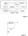
- Figure 1 illustrates a typical NQR system.
- the transmitter section used to excite the sample with the desired radio-frequency (RF); and a receiver section, used to detect the weak RF signals generated by the quadrupolar nuclei.
- the heart of the apparatus is the spectrometer, which performs both transmitter and receiver functions. Given a pulse sequence, the spectrometer, which contains an RF source and pulse modulation hardware, will produce RF pulses with the desired characteristics, ready for amplification by the RF power amplifier. The amplified pulse sequence is then transmitted to the sample via the probe.
- the probe consists of a shield, an RF antenna and the electronics required to tune the antenna to the correct excitation frequency and match its impedance to the other electronic devices.
- a shield big enough to house the coil and the tuning and matching circuitry, with an easily removable lid, is provided.
- the shield is not a Faraday shield, as it only shields the contents from electric fields and not magnetic fields.
- a crossed-diode is a nonlinear element because it looks like a good conductor for large incoming signals, but like a poor conductor to signals of either polarity. Therefore, putting crossed-diodes between the power amplifier and the probe means that the high power RF pulses are passed successfully to the probe, but at all other times the probe is isolated from the transmitter section and therefore also from any noise in the transmitter section.
- the receiver section consists of the RF antenna to measure the weak signals from the sample, a pre-amplification stage to enhance the weak signal, and hardware (within the spectrometer) used to demodulate the measured signal at the excitation frequency.
- a single antenna is provided for both transmit and receive. Since the transmitted RF pulses are several orders of magnitude greater than the received NQR signals, extra electronic circuitry is required in order to protect the sensitive receiver section during the RF pulse.
- the crossed-diodes to ground protect the sensitive receiver circuitry during an RF pulse, since during a pulse the cross-diodes act as a good conductor "shunting" the signal to ground. When the signal falls below the diode threshold voltage, the signal is passed to the rest of the receiver circuit.
- the shorted quarter wave cable, between the probe and the rest of the receiver section performs a kind of band pass filtering operation. It acts as an open circuit only for signals around the design frequency and will attenuate all others, thus helping to filter out unwanted noise.
- the Quality (Q) factor is a measure of the quality of a resonant system and is important, firstly, as the SNR is proportional to Q 1/2 , secondly, because the recovery time of the tuned circuit is proportional to the Q, and thirdly, because the bandwidth of the system is effected by it.
- the lower/upper cut-off frequency is defined as the frequency below/above which the output of the tuned circuit is reduced to 70.7% of the reference voltage at f_0.
- NQR signals can generally not be measured during or directly after the excitation pulses, as these pulses are many orders of magnitude greater in amplitude than the generated NQR signals, leading to a dead-time between the centre of the excitation pulse and the first sample. Rapid detection of signals that decay quickly in the time domain (and are broad in the frequency domain) is limited by the length of this dead-time, as the strongest part of the signal will have been lost in this time. The biggest contributor to this dead-time is the time required for the RF voltage, due to the excitation, to decay (or ring-down) to levels of the same order of magnitude as the NQR signals.
- the ring-down time is proportional to the Quality (Q) factor of the probe, so one possible option would be to lower the Q-factor of the probe; however, the SNR is proportional to Q 1/2 . Therefore, ideally one would like to lower the Q of the probe directly after the transmit pulse, in order to allow rapid ring-down of the residual transmit RF, then increase the Q when the NQR signal is sampled, in order to give a high SNR.
- the task of the Q damper is to allow rapid switching of the Q of the receiver circuit, as required.
- Figure 3 shows the circuit diagram of the Q-damper. It is noted that the values of the components R1, R2, C1 and C2 depend upon the specifications of the damping coil and the operating frequency. Further, Q1 and Q2 are BUP35 NPN transistors, D1 and D2 are STTA806D diodes, D3 is a BZX86C6V2 diode and MC34152P is a MOSFET Driver integrated circuit.
- This embodiment describes how, in noise spectroscopy, SOI-free correlation domain samples can be used to reduce the influence of corruptive signals. This is further discussed in Papers A.
- the SOI is obtained by cross-correlating the (pseudo white) noise excitation sequence with the time domain response, yielding the correlation domain signal. Often, however, only a very small portion of the correlation domain signal will contain the SOI; therefore, the rest of the signal can be considered SOI-free.
- the corrupting signals comprise of interference, belonging to a low rank linear subspace, embedded in white Gaussian noise.
- An estimate of the low rank linear subspace is formed from the signal-of-interest free samples and used to reduce the influence of the corruptive signals; the resulting algorithm is termed SEAQUER.
- the corruptive signal is assumed to be pure zero mean Gaussian noise.
- An estimate of the noise covariance matrix is formed from the signal-of-interest free samples, from which a prewhitening transform, which can be used to reduce the influence of the corruptive signals, is derived; the resulting algorithm is termed RCDAML.
- SEAQUER and RCDAML techniques are applicable to all forms of noise spectroscopy. Note that SEAQUER and RCDAML are examples of two ways of exploiting the SOI-free samples to reduce the influence of corrupting signals.
- Nuclear quadrupole resonance is a solid-state radio frequency (RF) spectroscopic technique, allowing the detection of compounds containing quadrupolar nuclei, a requirement fulfilled by many high explosives and narcotics.
- RF radio frequency
- the practical use of NQR is restricted by the inherently low signal-to-noise ratio of the observed signals, a problem that is further exacerbated by the presence of strong RF interference (RFI).
- the current literature focuses on the use of conventional, multiple-pulsed NQR (cNQR) to obtain signals.
- An alternative method called stochastic NQR (sNQR) is provided, having many advantages over cNQR, one of which is the availability of signal-of-interest free samples.
- these samples are exploited forming a matched subspace-type detector and a detector employing a pre-whitening approach, both of which are able to efficiently reduce the influence of RFI.
- many of the ideas already developed for cNQR including providing robustness to uncertainties in the assumed complex amplitudes and exploiting the temperature dependencies of the NQR spectral components, are recast for sNQR.
- the presented detectors are evaluated on both simulated and measured trinitrotoluene (TNT) data.
- Nuclear quadrupole resonance is a solid-state radio frequency (RF) technique that can be used to detect the presence of quadrupolar nuclei, such as the 14 N nucleus prevalent in many explosives and narcotics.
- RF radio frequency
- FID free induction decay
- NQR nuclear magnetic resonance
- sNQR trains of low power coherent pulses, whose phases or amplitudes are randomized, are used to interrogate the sample; herein, such pulses are termed stochastic pulses.
- stochastic pulses Providing sufficiently weak stochastic pulses are used, the NQR system maybe treated as linear and time invariant.
- cross-correlation of the observed time domain signal with a white input sequence yields the linear response (or FID) which may be well modelled as a sum of exponentially damped complex sinusoids.
- sNQR as compared to cNQR, is that significantly lower RF powers are required to achieve the same excitation bandwidth, which may be beneficial, for instance, in the area of humanitarian de-mining where lightweight, man-portable and battery-operated detectors are required, or for interrogating samples hidden on people, where there are strict limits on the amount of RF power that may be used.
- sNQR has an immediate advantage over cNQR when investigating compounds with long spin-lattice relaxation times, such as trinitrotoluene (TNT).
- TNT trinitrotoluene
- a restrictive delay usually five times the spin-lattice relaxation time, must be adhered to in between measurements, resulting in unfeasibly long detection times. This problem is alleviated in sNQR and data can (essentially) be acquired continuously.
- the bandwidth of the received signal is limited by the time between consecutive stochastic pulses, here termed the stochastic dwell time; for example, the bandwidth of the received signal is limited to, say, 25 kHz.
- the stochastic dwell time is limited by the time between consecutive stochastic pulses, here termed the stochastic dwell time; for example, the bandwidth of the received signal is limited to, say, 25 kHz.
- RF interference can be a major concern; e.g., in the detection of landmines containing TNT, the relatively weak NQR signal is significantly affected by radio transmissions in the AM radio band.
- extra RFI mitigation often needs to be employed, be it passive methods which use specially designed antennas to cancel far-field RFI, or active methods which require extra antennae to measure the background RFI .
- the FID will have decayed to negligible levels after five times the longest spin-phase memory decay time, here denoted T 2 , max ⁇ , which can be measured a priori.
- the spin-phase memory decay time of a resonant line can vary between samples, due to differing sample crystallinity and/or the presence of impurities.
- the spin-phase memory decay time is upper bounded by the spin-spin relaxation time, which does not change between samples, and could be used instead. Therefore, only a relatively small subset of the correlation domain data will contain the sNQR signal; however, RFI components will likely be present throughout the entire correlation domain.
- Section I-2 The data model for the correlation domain sNQR signal is outlined in Section I-2.
- Sections I-3 and I-4 contain the derivations for the SEAQUER and RCDAML algorithms, respectively.
- Section I-5 the performances of the proposed detectors are evaluated.
- Section I-6 draws some conclusions.
- the observed time domain signal will contain NP samples.
- Cross-correlation of the time domain signal with the (white) exciting sequence yields the correlation domain signal r ( t ), also consisting of NP samples, which may be well modelled as a gapped FID, consisting of evenly spaced blocks of data, sampled at the data dwell time, D w .
- MLBS maximum length binary sequence
- ⁇ k , ⁇ k ( T ) and ⁇ k denote the complex amplitude, the frequency shifting function and the sinusoidal damping constant of the k th FID component, respectively.
- w p ( t ) denotes an additive coloured noise, due to thermal (Johnson) noise and external RFI, where it is here assumed that any known noise colouring has already been removed. This is further discussed in Paper B.
- the maximum number of correlation blocks that should be used for estimation of the FID parameters are the first P ⁇ blocks that correspond to times less than or equal to 5 T 2 , max ⁇ .
- a subset of the remaining P-P ⁇ blocks, here selected as the last P ⁇ blocks, can then be used for interference and noise rejection.
- ( ⁇ ) T , ( ⁇ ) * , ( ⁇ ) ⁇ , ⁇ 2 , Re ⁇ and E ⁇ denote the transpose, the Hermitian transpose, the Moore-Penrose pseudoinverse, the two-norm, the real operator and the expectation operator, respectively.
- w N P ⁇ the coloured noise term, w N P ⁇
- w N P ⁇ S ⁇ + e N P ⁇
- S, ⁇ and e N P denoting the basis for the interference subspace, the interference subspace weights and an additive white Gaussian noise, respectively.
- the interference subspace will typically be unknown, and therefore must be estimated from the available data.
- Such an estimate may be formed by using the P ⁇ end correlation domain data blocks, by first constructing a N P ⁇ ⁇ P ⁇ / P ⁇ data matrix, X ⁇ , in which each column consists of P ⁇ end correlation domain data blocks.
- P ⁇ is selected as an integer multiple of P ⁇ .
- SVD singular value decomposition
- the interference consists of a mixture of either sinusoids or damped sinusoids, then the best choice for d int is as the number of sinusoidal components. If no prior knowledge of the number of RFI components is available, then a reasonable estimate may be obtained by examining the singular values of X ⁇ .
- PDF probability density function
- the data and model vectors are projected onto the space orthogonal to the interference subspace, nulling the effects of the interference.
- ⁇ is the common (real-valued) magnitude scaling due to the signal power
- ⁇ is the (complex) amplitude vector, normalized such that its largest magnitude equals unity, containing both the phases and the relative magnitudes of the d complex amplitudes.
- the magnitude errors, ⁇ k m are modelled as independent truncated Gaussian random variables, parameterized by the variance ⁇ m 2 .
- the phase errors, ⁇ k p are assumed to be independent identically distributed random variables, uniformly distributed over the interval [- P,P ], where 0 ⁇ P ⁇ ⁇ is selected according to the uncertainty in the phases.
- the statistics of the amplitude errors should be obtained from real measurements.
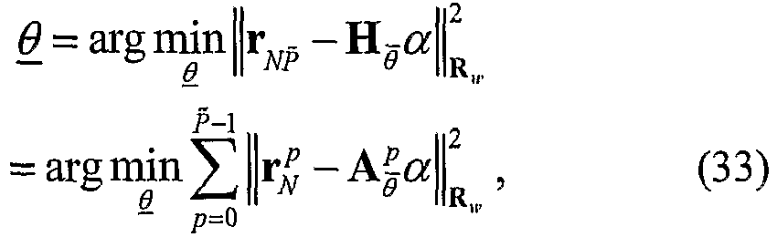
- an estimate of the vector best fitting the observed data can be obtained by solving the following constrained minimization min ⁇ ⁇ ⁇ S ⁇ ⁇ H ⁇ ⁇ ⁇ ⁇ r N P ⁇ ⁇ 2 2 subject to ⁇ ⁇ ⁇ ⁇ ⁇ ⁇ 2 2 ⁇ ⁇ , where ⁇ is here assumed known. It is noted that an initial estimate of ⁇ is needed to solve (20).
- the resulting detector is termed the SEAQUER detector.
- ⁇ Re H ⁇ ⁇ ⁇ ⁇ ⁇ ⁇ r ⁇ N P ⁇ .
- ⁇ ' is a predetermined threshold value reflecting the acceptable p f .
- the resulting detector the RCDAML detector. Similar to the SEAQUER detector, we resort to Monte-Carlo performance evaluation to determine ⁇ ' . t to the noise power. When there is RFI, the results illustrate that the detector is approximately CFAR with the respect to the unknown interference subspace and noise power.
- both the SEAQUER and RCDAML detectors require a ( d +1)-dimensional search over the nonlinear parameter space. This full search may be well approximated using ( d +1) one-dimensional searches, which may be iterated to further improve the fitting. This is further discussed in Paper B. Furthermore, for notational simplicity, we have here derived the SEAQUER and RCDAML detectors assuming the presence of only a single compound or polymorphic form.
- the measured data consisted of 1000 data files, 500 with TNT present and 500 without, each taking 30 seconds to acquire.
- the sample consisting of 180 g creamed monoclinic TNT, was placed inside a shielded solenoidal coil and maintained at a temperature of 295.15-296.15 K.
- the Quality (Q) factor of the coil and the pulse width were selected to ensure that the excitation bandwidth was sufficient to excite five v + lines of monoclinic TNT using a single excitation frequency of 843 kHz.
- MLBS maximum length binary sequence
- the table of Figure 5 summarizes the sNQR signal parameters, estimated from a high SNR signal, obtained by summing around 8 hours of data.
- the detectors were also compared on simulated data, with and without RFI.
- the simulated data without RFI, designed to mimic the measured data, was generated using (1), (2) together with the temperature shifting function constants for monoclinic TNT (see Figure 5).
- the RFI components were added to the time-domain sNQR signal, i.e., before cross-correlation.
- the RFI is modelled as a set of discrete sinusoids whose frequencies and phases are uniformly distributed (over the interval [- ⁇ , ⁇ ]), and with uniformly distributed (over the interval [0,1]) normalized magnitudes; here, six discrete sinusoids have been provided. It is noted that due to the chosen sampling rate, the RFI will always be within 25 kHz of the excitation frequency.
- DMA demodulation approaches
- P ⁇ 320 has been selected.
- the SEAQUER, RCDAML and DMA-s detectors use a search region over temperature of [290, 300] K (in 100 steps).
- the search regions could be restricted further, according to any prior knowledge concerning the sample's temperature and/or the sinusoidal dampings.
- the figure illustrates the benefits of the proposed SEAQUER and RCDAML algorithms, especially for ISR ⁇ 30 dB, where the effect of increasing the ISR on p d is negligible.
- the known and without error, and may be obtained by setting ⁇ 0.
- the standard SEAQUER algorithm selects ⁇ as E ⁇ ⁇ ⁇ , obtained using (20), (21) and Figure 5 .
- v the uncertainty parameter
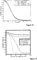
- Figure 9 shows f SEAQUER, p f vs. threshold curves for simulated data, generated using 3000 Monte-Carlo simulations.
- Figure 10 shows RCDAML, p f vs. threshold curves for simulated data, generated using 3000 Monte-Carlo simulations.
- the standard SEAQUER detector is compared with two special cases, denoted the SEAQUER-LS and SEAQUER- ⁇ 0 detectors.
- SEAQUER- ⁇ 0 performs well at low uncertainties when ⁇ represents the observed data well. Also, as expected, for high uncertainty, it is better to use SEAQUER-LS instead of the SEAQUER- ⁇ 0 as then ⁇ is significantly in error.
- the standard SEAQUER algorithm is able to perform better than both the special cases as it is able to exploit ⁇ , but also allow for errors in it. Studies illustrate similar results for the RCDAML detector.
- the stochastic NQR (sNQR) data model has been introduced and the benefits of sNQR as compared to conventional NQR have been discussed.
- SEAQUER stochastic NQR
- RCDAML two detection schemes
- the SEAQUER detector estimates a low-rank interference subspace, and exploits this in a matched subspace-type detector, whereas the RCDAML detector follows a pre-whitening approach, using a pre-whitening transform estimated from the data.
- the SEAQUER detector is shown to have the best interference and noise rejection capability.
- Performance studies using both simulated and measured sNQR data, indicate that the proposed methods show a significant performance gain as compared to existing techniques, allowing for an accurate detection even in the presence of substantial interference signals. Furthermore, numerical results illustrate that the presented detectors are CFAR with respect to the noise power, when RFI is absent, and approximately CFAR with respect to the unknown interference, when RFI is present.
- This embodiment describes how, in conventional spectroscopic methods, where the SOI is measured in the time domain, late SOI-free time-domain samples can be used to reduce the influence of corruptive signals.
- c-SEAQUER and RTDAML are examples of two ways of exploiting the SOI-free samples to reduce the influence of corrupting signals. Persons skilled in the art will appreciate that variants of the present invention may make use of other suitable algorithms.
- Nuclear Quadrupole Resonance is a solid-state radio frequency (RF) spectroscopic technique, allowing the detection of many high explosives and narcotics.
- RF radio frequency
- sNQR stochastic NQR
- cNQR conventional NQR
- the concept is closely related to the work in the first embodiment described above, although the algorithmic details differ sufficiently to make the extension non-trivial. Similar to the sNQR case, the presented detectors are able to substantially outperform all previously proposed cNQR detectors when RFI is present.
- Nuclear quadrupole resonance is a solid-state radio frequency (RF) technique that can be used to detect the presence of quadrupolar nuclei, such as the 14 N nucleus prevalent in many explosives and narcotics.
- RF interference can be a major concern; e.g., in the detection of landmines containing TNT, the relatively weak NQR signal is significantly affected by radio transmissions in the AM radio band.
- extra RFI mitigation needs to be employed, be it passive methods which use specially designed antennas to cancel far-field RFI, or active methods which require extra antennae to measure the background RFI.
- NQR data models used for conventional multiple-pulse NQR (cNQR) signals are significantly different to those used for sNQR, as are the acquisition processes.
- cNQR multiple-pulse NQR
- one cross-cor relates the NQR response with the white exciting signal to recover the SOI or the NQR free induction decay (FID). Since only a very small amount of the correlation domain signal will contain the FID, the remainder of the signal can be considered SOI-free, i.e., SOI-free signals arise naturally in sNQR.
- cNQR the SOI is acquired in the time domain.
- the SOI-free samples may be used to form an estimate of a subspace spanned by the RFI components and then cancel the influence of the RFI by projecting the SOI-data and cNQR model vectors onto the space orthogonal to this subspace.
- the SOI-free samples to derive a pre-whitening transform that can be used to remove the influence of RFI is exploited.
- the performance of the proposed algorithms will depend upon how stationary the RFI is in between the SOI and SOI-free data sets and therefore it is imperative to evaluate the algorithms using realistic RFI signals.
- the RFI has been modelled simplistically as a set of discrete sinusoids. This model is expanded to form a more realistic RFI model, so that it mimics the AM radio transmissions often present in real measurements.
- Section II-2 The data model for cNQR signals is outlined in Section II-2.
- Section 11-3 contains derivations for the c-SEAQUER algorithm.
- Section II-4 the performances of the proposed detectors are evaluated, before conclusions are drawn in Section II-5.
- ( ⁇ ) T , ( ⁇ ) * , ( ⁇ ) * , ⁇ 2 and Re ⁇ denote the transpose, the Hermitian transpose, the Moore-Penrose pseudoinverse, the two-norm and the real operator, respectively.
- M ⁇ SOI-free echoes are acquired, from which a N ⁇ M ⁇ data matrix, X ⁇ , is constructed. These SOI-free echoes are obtained after a delay of five times the longest spin-phase memory decay time after the last excitation pulse, by which time the NQR signal will have decayed to negligible levels. Excitation pulses should not continue to be applied, as this would result in having to wait for a considerably longer period (of five times the longest spin-echo decay time after the preparation pulse) for the NQR signal to decay to negligible levels.
- SVD singular value decomposition
- the number of RFI components will be unknown.
- ⁇ ⁇ is first factorized, where ⁇ is the common (real-valued) magnitude scaling due to the signal power, and ⁇ is the (complex) amplitude vector, normalized such that its largest magnitude equals unity. This is further discussed in Paper B.
- ⁇ the assumed (normalized) amplitude vector, here denoted ⁇ is considered, as well as the actual (normalized) amplitude vector, ⁇ , belong to an uncertainty hypersphere with radius ⁇ , i.e., ⁇ ⁇ ⁇ ⁇ ⁇ ⁇ 2 2 ⁇ ⁇ .
- an initial estimate of ⁇ is needed to solve (17).
- ⁇ max ⁇
- ⁇ ⁇ LS H ⁇ ⁇ ⁇ ⁇ z ⁇ NM is obtained by minimizing (15) with respect to ⁇ .
- GLRT generalized likelihood ratio
- c-SEAQUER The resulting detector is termed c-SEAQUER, where the "c” denotes conventional, to stress the difference to the sNQR version of the algorithm.
- c-SEAQUER requires a (2 d +1)-dimensional search over the nonlinear parameter space. This full search may be well approximated using (2 d +1) one-dimensional searches, which may be iterated to further improve the fitting. This is further discussed in Paper B.
- c-SEAQUER has been derived assuming the presence of only a single compound or polymorphic form.
- RCDAML Robust Time Domain Approximate Maximum Likelihood
- the performances of the proposed detectors are compared against current state-of-the-art detectors, namely the Robust Echo Train Approximate Maximum Likelihood (RETAML) and Frequency selective RETAML (FRETAML) algorithms, using simulated TNT data.
- RFI components are also added to the simulated data. Specifically, a variety of speech and audio signals are taked, sampled at 8 kHz (as for AM radio transmissions), and modulate the signals onto a carrier whose frequency is uniformly distributed over the interval [- ⁇ /4, ⁇ /4] (which corresponds to the RFI always being within 25 kHz of the excitation frequency).
- the resulting signal is then upsampled, according to the NQR sampling rate of 200 kHz, and added to the simulated NQR signal.
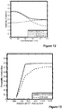
- Figure 11 illustrates the probability of detection ( p d ) vs the ISR, illustrating how the proposed algorithms are able to counter the RFI.
- the robustness to complex amplitude uncertainty is examined. Assuming a substantial interference of 60 dB, the c-SEAQUER detector is focused on, comparing it to two special cases, the c-SEAQUER-LS detector, which treats the complex amplitudes as unknown parameters, and the c-SEAQUER- ⁇ 0 detector, which exploits the relative complex amplitudes as known and without error. This is further discussed in Paper B.
- Figure 12 shows p d vs the uncertainty parameter, v, illustrating that the robust part of c-SEAQUER is unaffected by the presence of RFI.
- a technique is provided allowing for RFI in single-sensor cNQR measurements.
- the performances of these algorithms on realistic cNQR signals corrupted by typical AM RFI signals are evaluated.
- a representation of the corrupting signals, as modelled from noise characteristics determined from the SOI-free sample, can be simply subtracted in the frequency domain from the response signal.
Landscapes
- Physics & Mathematics (AREA)
- Spectroscopy & Molecular Physics (AREA)
- High Energy & Nuclear Physics (AREA)
- Condensed Matter Physics & Semiconductors (AREA)
- General Physics & Mathematics (AREA)
- Engineering & Computer Science (AREA)
- Signal Processing (AREA)
- Other Investigation Or Analysis Of Materials By Electrical Means (AREA)
- Magnetic Resonance Imaging Apparatus (AREA)
Description
- The present invention relates to the detection of species by Nuclear Quadrupole Resonance (NQR). In particular, there are described methods of exploiting signal of interest (SOI) free samples in single-sensor spectroscopic methods, to reduce the influence of corrupting signals. SOI-free samples are samples not containing the SOI (e.g. the NQR signal), but only corrupting signals, such as interference (e.g. RF interference), spurious signals (e.g. signals excited using the excitation itself, including signals related to ferromagnetic and piezoelectric effects), and high-rank noise (e.g., thermal noise).
- Nuclear quadrupole resonance (NQR) is a solid-state radio frequency (RF) spectroscopic technique that can be used to detect the presence of quadrupolar nuclei, such as the 14N nucleus prevalent in many explosives and narcotics. The practical use of NQR is restricted by the inherently low signal-to-noise ratio (SNR) of the observed signals, a problem that is further exacerbated by the presence of strong RF interference (RFI). In many NQR applications, RF interference (RFI) can be a major concern; for example, in the detection of landmines containing TNT, the relatively weak NQR signal is significantly affected by radio transmissions in the AM radio band. Often, extra RFI mitigation needs to be employed, be it passive methods which use specially designed antennas to cancel far-field RFI, or active methods which require extra antennae to measure the background RFI.
- The present invention aims to provide a method of reducing the effects of this interference and/or other 'corrupting' signals. Methods applicable to conventional NQR and stochastic NQR are described. These methods may also find application in other forms of noise spectroscopy, such as stochastic NMR (nuclear magnetic resonance) and EPR (electron paramagnetic resonance), and in other forms of conventional spectroscopy, e.g., NMR and EPR.
- International Patent Application
WO 96/26453 - Further information may be found in the documents:
- ▪ "Signal Processing Applications of Oblique Projection Operators," by R. T. Behrens and L. L. Scharf, IEEE Transactions on Signal Processing, vol. 42, no. 6, pp. 1413-1424, June 1994
- ▪ "Matched Subspace Detectors," by L. L. Scharf and B. Friedlander, IEEE Transactions on Signal Processing, vol. 42, no. 8, pp. 2146-2157, August 1994.
- ▪ "Detection of Stochastic Nuclear Quadrupole Resonance Signals", by S.D. Somasundaram et al., Digital Signal Processing, IEEE, pp. 367-370, 2007. This article describes a method of testing for the presence of a species within a sample by means of detecting stochastic nuclear quadrupole resonance signals, wherein a resonance response signal is detected by taking multiple samples between consecutive excitation pulses and cross-correlating the spectroscopic resonance inducing signal with the response signal.
- The following papers are from some of the inventors:
- ▪ Papers A
- ∘ "Robust Detection of Stochastic Nuclear Quadrupole Resonance Signals," by S. D. Somasundaram, A. Jakobsson, M.D. Rowe, J.A.S. Smith, N.R. Butt and K. Althoefer, IEEE Trans. On Signal Processing, vol. 56, no. 9, pp.4221-4229, September 2008.
- ∘ "Countering Radio Frequency Interference in Single-Sensor Quadrupole Resonance," by S. D. Somasundaram, A. Jakobsson and N.R. Butt, IEEE Geoscience and Remote Sensing Letters, vol. 6, no. 1, pp. 62-66, January 2009.
- ▪ Paper B
∘ "Robust Nuclear Quadrupole Resonance Signal Detection Allowing for Amplitude Uncertainties," by S. D. Somasundaram, A. Jakobsson, and E. Gudmundson, IEEE Trans. On Signal Processing, vol. 56, no. 3, pp. 887-894, March 2008. - According to a first aspect of the invention, there is provided a method of testing for the presence of a species within a sample comprising the steps of:
- applying a spectroscopic resonance inducing excitation to the sample, wherein the excitation is a stochastic excitation, such as a random or pseudo-random excitation;
- detecting a response signal from the sample by taking multiple samples between consecutive excitation pulses, the resonance response signal comprising a signal-of-interest of the species and at least one corrupting signal comprising radio frequency interference, emanating externally to the sample;
- cross-correlating the spectroscopic resonance inducing signal with the response signal to produce a correlation domain signal;
- processing a first part of the response signal comprising a signal-of-interest and a said corrupting signal and a second part of the response signal comprising solely a said corrupting signal, the corrupting signal being of the same type in the first and second parts; and
- determining from the second part of the response signal, information regarding the at least one corrupting signal, and using the information to form a model of the corrupting signal;
- projecting the model of the corrupting signal onto the first part f the response signal to null the effects of the corrupting signal in the first part of the response signal;
- and then using the correlation domain signal o derive a detector configured to determine the presence of the signal-of-interest from the first part of the response signal, when a predetermined threshold is exceeded.
- As used herein, the term "response signal" includes a signal detected directly as a result of the excitation and a signal which has been processed subsequent to its initial detection. Hence, for example, "response signal" includes that obtained in stochastic techniques, wherein the response characteristic is reconstructed from the individual responses to a series of small excitations.
- The method may be used to detect the NQR response from the 14N nucleus as found, for example, in explosives such as TNT or in narcotics such as cocaine and to all other quadrupolar nuclei, such as 35Cl in pharmaceutical analysis, 27Al in clay and other minerals, and 75As in toxic waste in abandoned land-fill. The method may also be used to detect the presence of a particular species within the sample. The method may also be used, for example, to distinguish between real and counterfeit medicines and to check on shelf life.
- The applied excitation may be a radio-frequency excitation. Preferably, this excites a nuclear quadrupole resonance (NQR) response in the sample. Alternatively, the excitation may excite nuclear magnetic resonance or alternatively electron paramagnetic resonance in the sample.
The correlation-domain response signal may be analogous to the free-induction decay (FID) signal obtained in cNQR. - Stochastic NQR (sNQR) has the advantage over conventional NQR (cNQR) in that substantially lower power excitation can be used, allowing for safer, more portable operation, and that data can be essentially collected continuously (in cNQR, the data collection rate is slowed and therefore detection time lengthened by samples with large spin-lattice relaxation times).
- Preferably, for sNQR, the response signal is sampled (i.e. data collected) using multiple-point acquisition i.e. by taking multiple samples between consecutive excitation pulses. Preferably, unlike in the prior art, algorithms are used to estimate spectral parameters directly from the resulting correlation-domain signal. This has the advantage, unlike in the prior art, that it is not necessary to perform repeat measurements in order to construct a complete gap-less correlation-domain signal i.e. data can (essentially) be acquired continuously.
- In any embodiment, the first part of the response signal may comprise a signal of interest (SOI) and 'corrupting' signal such as an interference signal and/or noise; the second part of the response signal may comprise substantially or solely a corrupting signal such as an interference signal and/or noise. Typically the corrupting signal is of the same type in the first and second parts.
- The 'corrupting' signal may be interference, such as radio-frequency interference, spurious signals or high-rank or thermal noise.
- Preferably, the SOI is relatively strong, or non-negligible, in the first part of the response signal and relatively weak, or substantially negligible, in the second part of the response signal. Between the first and second parts of the response signal may be an intermediate region of the response signal wherein the SOI is either strong or non-negligible. Preferably this intermediate region of the response signal is not used in the processing step and/or is not detected.
- Preferably, the start of the first part of the response signal is at a period after the ring-down time of the sample, as known or measured a priori.
- Alternatively, and preferably in the case of sNQR, ringdown effects may be suppressed by means of Q-damping circuitry, phase cycling and the technique of composite pulses.
- Preferably, the end of the first part of the response signal is at a period after the associated excitation (for example, excitation pulse) which is less than five times, preferably less than three times, more preferably less than twice, and yet more preferably less than the longest spin-phase
decay time 

- It will be understood that the concept of a time axis as used in describing the signals and responses of conventional NQR (cNQR) in the time domain is analogous to a cross-correlation lag axis as used in stochastic NQR (sNQR) in the cross-correlation domain, and that the use of 'time' (including the
quantity 
- It is to be understood that wherever the
term 
art 
- Preferably, the start of the second part of the response signal is at a period after the associated excitation which is more than at least one, two, three or five times the longest spin-phase
decay time 
- Preferably, the start of the second part is at a period after the start of the first part that is more than 1, 2, 3, or 5 times the duration of the first part.
- Preferably, the method further comprises processing the second part of the response signal in order to obtain a model of the corrupting signal. Preferably, the model of the corrupting signal is used to reduce the effects of the corrupting signal in the first part of the response signal.
- Preferably, for stochastic NQR (sNQR), the resulting correlation-domain signal is modelled as a gapped free-induction decay (FID). Algorithms may be used to estimate the required parameters directly from the 'gapped' data.
- The corrupting signal may be modelled as belonging to a low-rank linear subspace, embedded in wideband noise, and the second part of the response signal may be used to make an estimate of this low-rank linear subspace, and may be used in reducing the influence of the corrupting signal in the part of the response signal containing the SOI.
- Alternatively, the corrupting signal may be modelled as pure zero mean Gaussian noise, and the second part of the response signal may be used to estimate the corresponding noise covariance matrix and thus allow the construction of a pre-whitening transform for use in reducing the influence of the corruptive signal in the part of the response signal containing the SOI.
- Preferably, other parts of the response signal may also be modelled, including, for example the first part of the response signal, which is to say the SOI with the corrupting signal.
- Preferably, the model of the corrupting signal may be used to adjust the model of the first part of the response signal.
- Preferably, spurious signals are reduced by repeating the excitation at cycled phases, for example as taught in International Patent Application No.
PCT/GB96/00422 - Preferably, only a single sensor is used. That is, the design is preferably non-gradiometric.
- The invention also provides apparatus with which to put into effect the methods of the present invention, as defined in claim 8. Preferably, this consists of a transmitter, with which to excite the sample, and a receiver with which to detect the response signal. Transmitting and receiving functions may be combined. Preferably, the transmitter comprises an RF source, pulse modulator, an RF power amplifier, and a probe. The probe may consist of a shield, an RF antenna and tuning electronics.
- A processor, associated memory and storage may also be provided.
- Any feature in one aspect of the invention may be applied to other aspects of the invention, in any appropriate combination, provided such a combination is covered by the claims. In particular, method aspects may be applied to apparatus aspects, and vice versa.
- Furthermore, features implemented in hardware may generally be implemented in software, and vice versa. Any reference to software and hardware features herein should be construed accordingly.
- It will be understood that the present invention as described below is purely by way of example; modifications of detail can be made within the scope of the invention, as defined by the appended claims.
- These and other aspects of the present invention will become apparent from the following exemplary embodiments that are described with reference to the accompanying figures in which:
-
Figure 1 is a block diagram of an NQR system; -
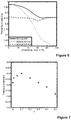
Figure 2 is a schematic diagram of the tuning and matching circuitry; -
Figure 3 is a circuit diagram of the Q-damper; -
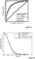
Figure 4 is a graph showing the probability of detection as a function of the ISR, for pf = 0.05, using simulated data with SNR = -34 dB; -
Figure 5 is a table showing estimates of sNQR signal parameters for the d = 5 v + lines of monoclinic TNT, for an excitation frequency of 843 kHz, in the region of 830-860 kHz; -
Figure 6 is a graph showing the probability of detection as a function of the uncertainty level, for pf = 0.1, using simulated data with SNR=-34 dB and ISR = 60 dB; -
Figure 7 is a graph showing a plot of pd vs ε, for pf = 0.02, using measured data; -
Figure 8 is a graph showing the ROC curves for measured data, with (where applicable) ε = 0.1; -
Figure 9 is a graph showing for SEAQUER, pf vs. threshold curves for simulated data, generated using 3000 Monte-Carlo simulations; -
Figure 10 is a graph showing for RCDAML, pf vs. threshold curves for simulated data, generated using 3000 Monte-Carlo simulations; -
Figure 11 is a graph showing (for the second embodiment) the probability of detection as a function of the ISR, for pf = 0.05, using simulated data with SNR = -27 dB; -
Figure 12 is a graph showing (for the second embodiment) the probability of detection as a function of the uncertainty parameter, v, for pf = 0.02, using simulated data with SNR = -27 dB and ISR = 60dB; and -
Figure 13 is a graph showing (for the second embodiment) the probability of detection as a function of
-
Figure 1 illustrates a typical NQR system. There are two main sections: the transmitter section, used to excite the sample with the desired radio-frequency (RF); and a receiver section, used to detect the weak RF signals generated by the quadrupolar nuclei. The heart of the apparatus is the spectrometer, which performs both transmitter and receiver functions. Given a pulse sequence, the spectrometer, which contains an RF source and pulse modulation hardware, will produce RF pulses with the desired characteristics, ready for amplification by the RF power amplifier. The amplified pulse sequence is then transmitted to the sample via the probe. The probe consists of a shield, an RF antenna and the electronics required to tune the antenna to the correct excitation frequency and match its impedance to the other electronic devices. In one embodiment, in order to develop and test many of the algorithms, it was necessary to obtain data without external RFI. Therefore, a shield big enough to house the coil and the tuning and matching circuitry, with an easily removable lid, is provided. The shield is not a Faraday shield, as it only shields the contents from electric fields and not magnetic fields. -
Figure 2 shows the schematic diagram of the circuitry needed to tune the RF antenna to the excitation frequency, and match the impedance of the probe to the rest of the hardware. It is noted that variable capacitors were used for both tuning, Ct, and matching, Cm. The total capacitance (Cm+Ct) needed to tune the probe to a given frequency is given by
- The receiver section consists of the RF antenna to measure the weak signals from the sample, a pre-amplification stage to enhance the weak signal, and hardware (within the spectrometer) used to demodulate the measured signal at the excitation frequency. A single antenna is provided for both transmit and receive. Since the transmitted RF pulses are several orders of magnitude greater than the received NQR signals, extra electronic circuitry is required in order to protect the sensitive receiver section during the RF pulse. The crossed-diodes to ground protect the sensitive receiver circuitry during an RF pulse, since during a pulse the cross-diodes act as a good conductor "shunting" the signal to ground. When the signal falls below the diode threshold voltage, the signal is passed to the rest of the receiver circuit. The shorted quarter wave cable, between the probe and the rest of the receiver section, performs a kind of band pass filtering operation. It acts as an open circuit only for signals around the design frequency and will attenuate all others, thus helping to filter out unwanted noise.
- The Quality (Q) factor is a measure of the quality of a resonant system and is important, firstly, as the SNR is proportional to Q1/2, secondly, because the recovery time of the tuned circuit is proportional to the Q, and thirdly, because the bandwidth of the system is effected by it. In a tuned RF receiver circuit, the Q is defined as


- A useful expression for measuring the Q of a tuned circuit is
- NQR signals can generally not be measured during or directly after the excitation pulses, as these pulses are many orders of magnitude greater in amplitude than the generated NQR signals, leading to a dead-time between the centre of the excitation pulse and the first sample. Rapid detection of signals that decay quickly in the time domain (and are broad in the frequency domain) is limited by the length of this dead-time, as the strongest part of the signal will have been lost in this time. The biggest contributor to this dead-time is the time required for the RF voltage, due to the excitation, to decay (or ring-down) to levels of the same order of magnitude as the NQR signals. The ring-down time is proportional to the Quality (Q) factor of the probe, so one possible option would be to lower the Q-factor of the probe; however, the SNR is proportional to Q1/2. Therefore, ideally one would like to lower the Q of the probe directly after the transmit pulse, in order to allow rapid ring-down of the residual transmit RF, then increase the Q when the NQR signal is sampled, in order to give a high SNR. The task of the Q damper is to allow rapid switching of the Q of the receiver circuit, as required.
-
Figure 3 shows the circuit diagram of the Q-damper. It is noted that the values of the components R1, R2, C1 and C2 depend upon the specifications of the damping coil and the operating frequency. Further, Q1 and Q2 are BUP35 NPN transistors, D1 and D2 are STTA806D diodes, D3 is a BZX86C6V2 diode and MC34152P is a MOSFET Driver integrated circuit. - This embodiment describes how, in noise spectroscopy, SOI-free correlation domain samples can be used to reduce the influence of corruptive signals. This is further discussed in Papers A.
- In stochastic/noise spectroscopy, the SOI is obtained by cross-correlating the (pseudo white) noise excitation sequence with the time domain response, yielding the correlation domain signal. Often, however, only a very small portion of the correlation domain signal will contain the SOI; therefore, the rest of the signal can be considered SOI-free.
- Two examples of exploiting SOI-free samples in stochastic NQR are described. In one example it is assumed that the corrupting signals comprise of interference, belonging to a low rank linear subspace, embedded in white Gaussian noise. An estimate of the low rank linear subspace is formed from the signal-of-interest free samples and used to reduce the influence of the corruptive signals; the resulting algorithm is termed SEAQUER. In the second example, the corruptive signal is assumed to be pure zero mean Gaussian noise. An estimate of the noise covariance matrix is formed from the signal-of-interest free samples, from which a prewhitening transform, which can be used to reduce the influence of the corruptive signals, is derived; the resulting algorithm is termed RCDAML.
- This invention and the SEAQUER and RCDAML techniques are applicable to all forms of noise spectroscopy. Note that SEAQUER and RCDAML are examples of two ways of exploiting the SOI-free samples to reduce the influence of corrupting signals.
- Nuclear quadrupole resonance (NQR) is a solid-state radio frequency (RF) spectroscopic technique, allowing the detection of compounds containing quadrupolar nuclei, a requirement fulfilled by many high explosives and narcotics. The practical use of NQR is restricted by the inherently low signal-to-noise ratio of the observed signals, a problem that is further exacerbated by the presence of strong RF interference (RFI). The current literature focuses on the use of conventional, multiple-pulsed NQR (cNQR) to obtain signals. An alternative method called stochastic NQR (sNQR) is provided, having many advantages over cNQR, one of which is the availability of signal-of-interest free samples. In this embodiment, these samples are exploited forming a matched subspace-type detector and a detector employing a pre-whitening approach, both of which are able to efficiently reduce the influence of RFI. Further, many of the ideas already developed for cNQR, including providing robustness to uncertainties in the assumed complex amplitudes and exploiting the temperature dependencies of the NQR spectral components, are recast for sNQR. The presented detectors are evaluated on both simulated and measured trinitrotoluene (TNT) data.
- Nuclear quadrupole resonance (NQR) is a solid-state radio frequency (RF) technique that can be used to detect the presence of quadrupolar nuclei, such as the 14N nucleus prevalent in many explosives and narcotics. Historically, the linear response of the NQR system known as the free induction decay (FID) was measured, using a simple one-pulse experiment; however, since the advent of multiple-pulse techniques, the trend has instead been to obtain nonlinear responses, enabling signals with higher signal-to-noise ratios (SNRs) to be obtained in a shorter time . The aforementioned acquisition methods, which are termed collectively as conventional NQR (cNQR) methods, use powerful coherent RF modulated pulses to interrogate the sample. An alternative method for acquiring NQR signals, called stochastic NQR (sNQR), uses stochastic (or noise) excitation . Whilst stochastic excitation was proposed for nuclear magnetic resonance (NMR) as early as 1970 , there are still relatively few publications on stochastic NMR.
- In sNQR, trains of low power coherent pulses, whose phases or amplitudes are randomized, are used to interrogate the sample; herein, such pulses are termed stochastic pulses. Providing sufficiently weak stochastic pulses are used, the NQR system maybe treated as linear and time invariant. Thus, cross-correlation of the observed time domain signal with a white input sequence yields the linear response (or FID) which may be well modelled as a sum of exponentially damped complex sinusoids.
- An important advantage of sNQR, as compared to cNQR, is that significantly lower RF powers are required to achieve the same excitation bandwidth, which may be beneficial, for instance, in the area of humanitarian de-mining where lightweight, man-portable and battery-operated detectors are required, or for interrogating samples hidden on people, where there are strict limits on the amount of RF power that may be used.
- Furthermore, sNQR has an immediate advantage over cNQR when investigating compounds with long spin-lattice relaxation times, such as trinitrotoluene (TNT). In cNQR, a restrictive delay, usually five times the spin-lattice relaxation time, must be adhered to in between measurements, resulting in unfeasibly long detection times. This problem is alleviated in sNQR and data can (essentially) be acquired continuously.
- It is noted that although broadband excitation has been shown to be achievable for sNQR, a limitation of previous work is that the bandwidth of the received signal is limited by the time between consecutive stochastic pulses, here termed the stochastic dwell time; for example, the bandwidth of the received signal is limited to, say, 25 kHz. This as previous techniques acquired only a single data point between consecutive stochastic pulses, a technique here termed as single-point acquisition, and therefore the sampling period is equal to the stochastic dwell time. Due to effects such as ringdown, there is a limit on how short one can make the stochastic dwell time (and thus also the sampling period when single-point acquisition is used). It has been shown, for both NMR and electron paramagnetic resonance (EPR), that the spectral bandwidth can be increased by acquiring two or more data points between consecutive pulses. Herein, such a technique is employed for sNQR, here termed as multiple-point acquisition. The resulting correlation domain signal can then be well modeled as an FID with periodically recurring gaps. In the prior art, for NMR, it is proposed to handle these gaps by repeating the measurements with differing experimental settings so that the gaps occur in different places, and then stitching the resulting gapped FIDs together to form a single seamless FID. Rather, algorithms are provided that are able to estimate the required spectral parameters directly from the gapped data.
- In many NQR applications, RF interference (RFI) can be a major concern; e.g., in the detection of landmines containing TNT, the relatively weak NQR signal is significantly affected by radio transmissions in the AM radio band. In cNQR, extra RFI mitigation often needs to be employed, be it passive methods which use specially designed antennas to cancel far-field RFI, or active methods which require extra antennae to measure the background RFI . For sNQR, however, it is possible to cancel the effects of the RFI without the need for these additional techniques. It is noted that the FID will have decayed to negligible levels after five times the longest spin-phase memory decay time, here denoted

- One alternative is to use the correlation domain samples known not to contain NQR components, here termed the signal-of-interest free samples, to obtain an estimate of the noise covariance matrix, and then use this to pre-whiten any unknown noise coloring; such an approach leads to the here proposed Robust Correlation Domain Approximate Maximum Likelihood (RCDAML) detector.
- Another alternative is to assume that the RFI lies in a low-rank linear interference subspace that can be estimated from the signal-of-interest free samples. The interference subspace is then exploited to form a matched subspace-type detector. This approach yields the Subspace-based EvaluAtion of QUadrupole resonance signals Exploiting Robust methods (SEAQUER) detector introduced in Section I-3.
- Furthermore, we beneficially exploit the dependencies of the NQR frequencies on temperature when forming both the SEAQUER and RCDAML detectors. Additionally, it has been shown to be beneficial to exploit prior knowledge concerning the complex amplitudes of the NQR components, which allows such information to be exploited, but also allows for uncertainty in it. This is further discussed in Paper B.
- The data model for the correlation domain sNQR signal is outlined in Section I-2. Sections I-3 and I-4 contain the derivations for the SEAQUER and RCDAML algorithms, respectively. In Section I-5, the performances of the proposed detectors are evaluated. Finally, Section I-6 draws some conclusions.
- If the sample is interrogated with a stochastic excitation sequence consisting of P stochastic pulses, and N samples are acquired after each pulse, then the observed time domain signal will contain NP samples. Cross-correlation of the time domain signal with the (white) exciting sequence, yields the correlation domain signal r(t), also consisting of NP samples, which may be well modelled as a gapped FID, consisting of evenly spaced blocks of data, sampled at the data dwell time, Dw. It is noted that if a pseudo random noise sequence such as the maximum length binary sequence (MLBS) is used for excitation, then the fast Hadamard transform can be used for cross-correlation. The p th correlation domain block may then be written as


- The maximum number of correlation blocks that should be used for estimation of the FID parameters are the first P̃ blocks that correspond to times less than or equal to


- In the following, (·) T , (·)*, (·)†, ∥·∥2, Re{·} and E{·} denote the transpose, the Hermitian transpose, the Moore-Penrose pseudoinverse, the two-norm, the real operator and the expectation operator, respectively.
- Using (1), the pth data block may be expressed as


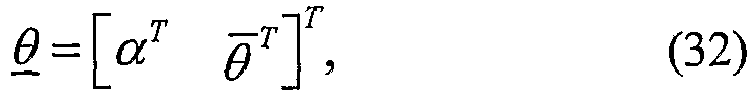
θ =[T βT ] T and β = [β 1 βd ] T denoting the nonlinear parameter vector and the vector of unknown sinusoidal dampings, respectively. Thus, the data model for P̃ data blocks can be written as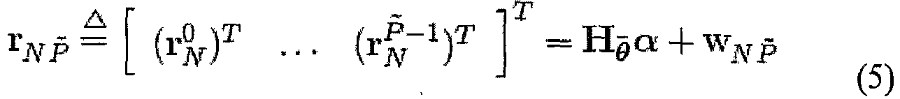

- Here, it is further assumed that the coloured noise term, w N P̃ , may be factored as

P denoting the basis for the interference subspace, the interference subspace weights and an additive white Gaussian noise, respectively. Thus, (5) may be rewritten as
- It is noted that the interference subspace will typically be unknown, and therefore must be estimated from the available data. Such an estimate may be formed by using the


int , i.e.,


- Minimizing (12) with respect to φ yields an estimate of φ as


- Thus, the data and model vectors are projected onto the space orthogonal to the interference subspace, nulling the effects of the interference.
- To exploit the prior knowledge typically available for the complex amplitudes,

- Is first factorized, where ρ is the common (real-valued) magnitude scaling due to the signal power, and κ is the (complex) amplitude vector, normalized such that its largest magnitude equals unity, containing both the phases and the relative magnitudes of the d complex amplitudes. This is further discussed in Paper B. It is here considered the case when the assumed (normalized) amplitude vector, here denoted
κ , as well as the actual (normalized) amplitude vector, κ, belong to an uncertainty hypersphere with radius
- The choice of ε should reflect the uncertainty in the complex amplitudes, typically obtained as a result of the experimental setup. Herein, as further discussed in Paper B, ε is modelled as a random variable, ε , formed as


κ k | and ∠κ k denoting the assumed magnitude and phase components;


variance 

- By restricting the actual (normalized) amplitude vector to this hypersphere, an estimate of the vector best fitting the observed data can be obtained by solving the following constrained minimization

θ is here assumed known. It is noted that an initial estimate of ρ is needed to solve (20). By noting that ρ is the largest magnitude in α, an initial estimate of ρ may be obtained as


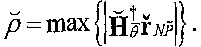
- Given κ̂, ρ may be re-estimated as

- Forming


θ to stress the dependence of α̂ onθ . In general, the nonlinear parameter vector,θ , will be unknown and must be estimated by minimizing ϕθ overθ , using a grid search. Thus, for each value ofθ , the residual error, ϕθ , is evaluated using (20)-(28). The estimated value ofθ is then found as the parameter vector minimizing this error, i.e.,
- The test statistic is formed as an (approximate) generalized likelihood ratio (GLRT) detector, i.e.


- In this section, the RCDAML algorithm is derived in which a pre-whitening approach for interference rejection is employed. Let R w denote the covariance matrix of the additive noise term, i.e.,

- Then, using (5), the maximum likelihood estimate of


-
Figure 4 shows the probability of detection as a function of the ISR, for pf = 0.05, using simulated data with SNR = -34 dB.
Factorizing


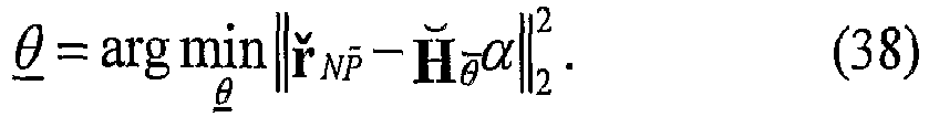
- Factorizing α as in (16), a robust estimate of κ may be found by solving the constrained minimization


- Forming


θ . Thus, similar to the SEAQUER detector, an estimate of the nonlinear parameter vector is obtained as
θ ,


- We remark that both the SEAQUER and RCDAML detectors require a (d+1)-dimensional search over the nonlinear parameter space. This full search may be well approximated using (d+1) one-dimensional searches, which may be iterated to further improve the fitting. This is further discussed in Paper B. Furthermore, for notational simplicity, we have here derived the SEAQUER and RCDAML detectors assuming the presence of only a single compound or polymorphic form. In previous work, we have shown (for cNQR) that when multiple polymorphs/compounds are present, it is beneficial to combine the signals from all contained components, and we have outlined an approach for dealing with multiple components of a mixture, whilst also allowing for robustness in the assumed amplitudes associated with each compound/polymorph.
-
Figure 5 shows a table of estimates of sNQR signal parameters for the d = 5 v + lines of monoclinic TNT, for an excitation frequency of 843 kHz, in the region of 830-860 kHz. - In this section the performance of the proposed detectors using both simulated and measured sNQR data is examined. The measured data consisted of 1000 data files, 500 with TNT present and 500 without, each taking 30 seconds to acquire. The sample, consisting of 180 g creamed monoclinic TNT, was placed inside a shielded solenoidal coil and maintained at a temperature of 295.15-296.15 K. The Quality (Q) factor of the coil and the pulse width were selected to ensure that the excitation bandwidth was sufficient to excite five v + lines of monoclinic TNT using a single excitation frequency of 843 kHz. A length P = 511 stochastic excitation sequence was used, in which the phases of the RF pulses were randomized with either 0 or 180° phase shifts, using a maximum length binary sequence (MLBS). For each 30 s data file, this sequence was repeatedly applied, and the responses from each sequence summed up. Following each stochastic pulse, N = 64 data points were acquired, where Dw = 2×10⁻⁵ s, yielding a time domain sequence consisting of NP = 32704 samples. This time-domain signal was then cross-correlated using the fast Hadamard transform to obtain the correlation domain signal. In our experiments, Q-damping circuitry, phase cycling and the technique of composite pulses were used to suppress ringdown effects. The table of
Figure 5 summarizes the sNQR signal parameters, estimated from a high SNR signal, obtained by summing around 8 hours of data. The detectors were also compared on simulated data, with and without RFI. The simulated data without RFI, designed to mimic the measured data, was generated using (1), (2) together with the temperature shifting function constants for monoclinic TNT (seeFigure 5). For the simulations with RFI, the RFI components were added to the time-domain sNQR signal, i.e., before cross-correlation. -
Figure 6 shows the probability of detection as a function of the uncertainty level, for pf = 0.1, using simulated data with SNR = -34 dB and ISR = 60 dB.
The RFI is modelled as a set of discrete sinusoids whose frequencies and phases are uniformly distributed (over the interval [-π,π]), and with uniformly distributed (over the interval [0,1]) normalized magnitudes; here, six discrete sinusoids have been provided. It is noted that due to the chosen sampling rate, the RFI will always be within 25 kHz of the excitation frequency. The interference-to-(noise-free) NQR signal ratio (ISR) is here defined as


-
Figure 7 shows a plot of pd vs ε, for pf = 0.02, using the measured data.
Initially, the interference rejection capabilities of the algorithms is examined. As a reference, the presented detectors to the demodulation approaches (DMA), which measure the response of a single resonance frequency is also compared. The DMA-p detector is allowed perfect knowledge of the sample's temperature so that the location of the most dominant resonance is exactly known. However, for applications such as landmine detection, it is difficult to estimate the sample's temperature with more than 5 K accuracy; therefore, the R̂ w = I is also included, corresponding to the case of no interference rejection. - It is noted that the spin-phase memory decay time for the kth resonance, here denoted


Figure 5 , we note that

Figure 4 illustrates the probability of detection (pd ) as a function of the ISR, for simulated data with RFI, where the uncertainty in the complex amplitudes is selected as zero and therefore ε = 0. The figure illustrates the benefits of the proposed SEAQUER and RCDAML algorithms, especially for ISR ≥ 30 dB, where the effect of increasing the ISR on pd is negligible. It is noted that for low ISR, theκ , and can be obtained either by setting ε = ∞, or by using (24), instead of (29), in (30). The known and without error, and may be obtained by setting ε = 0. The standard SEAQUER algorithm selects ε as E{ ε }, obtained using (20), (21) andFigure 5 . We define the uncertainty parameter v, which couples the uncertainties in the phases and the magnitudes. This is further discussed in Paper B. For a given value of v, we set
Figure 6 illustrates, for simulated data with RFI, the effect of varying the uncertainties in the complex amplitudes, indicating that the robust part of the SEAQUER detectors is unaffected by the presence of RFI. -
Figure 8 shows the ROC curves for measured data, with (where applicable) ε = 0.1. -
Figure 9 shows f SEAQUER, pf vs. threshold curves for simulated data, generated using 3000 Monte-Carlo simulations. -
Figure 10 shows RCDAML, pf vs. threshold curves for simulated data, generated using 3000 Monte-Carlo simulations. - For comparison, the standard SEAQUER detector is compared with two special cases, denoted the SEAQUER-LS and SEAQUER-ε0 detectors. The SEAQUER-LS detector represents the case when no prior knowledge of the complex amplitudes is exploited, i.e. it does not exploit
κ , and can be obtained by setting ε = ∞. The SEAQUER-ε0 detector represents the case when the relative complex amplitudes are exploited as known and without error, and may obtained by setting ε = 0. - As expected, SEAQUER-ε0 performs well at low uncertainties when
κ represents the observed data well. Also, as expected, for high uncertainty, it is better to use SEAQUER-LS instead of the SEAQUER-ε0 as thenκ is significantly in error. The standard SEAQUER algorithm is able to perform better than both the special cases as it is able to exploitκ , but also allow for errors in it. Studies illustrate similar results for the RCDAML detector. - The measured data, obtained under laboratory conditions, is examined; hence, it can be expected that the uncertainty in the complex amplitudes to be low.
Figure 7 illustrates pd as a function of ε for the real data, illustrating that even under laboratory conditions, it is beneficial to allow for errors in the assumed complex amplitudes. Furthermore, as is clear from the figure, the algorithm is quite robust to the actual choice of ε, indicating that the assumed uncertainty level does not need to be known precisely. As detection is the problem of interest, the receiver operating characteristic (ROC) curves for the SEAQUER, RCDAML are examined. - In this embodiment, the stochastic NQR (sNQR) data model has been introduced and the benefits of sNQR as compared to conventional NQR have been discussed. Furthermore, two detection schemes have been provided, termed SEAQUER and RCDAML, that are robust to the presence of RFI, typically observed in practical scenarios. The SEAQUER detector estimates a low-rank interference subspace, and exploits this in a matched subspace-type detector, whereas the RCDAML detector follows a pre-whitening approach, using a pre-whitening transform estimated from the data. Of the two, the SEAQUER detector is shown to have the best interference and noise rejection capability. Performance studies, using both simulated and measured sNQR data, indicate that the proposed methods show a significant performance gain as compared to existing techniques, allowing for an accurate detection even in the presence of substantial interference signals. Furthermore, numerical results illustrate that the presented detectors are CFAR with respect to the noise power, when RFI is absent, and approximately CFAR with respect to the unknown interference, when RFI is present.
- This embodiment describes how, in conventional spectroscopic methods, where the SOI is measured in the time domain, late SOI-free time-domain samples can be used to reduce the influence of corruptive signals.
- Two examples of exploiting signal of interest free samples in conventional NQR are described. One example closely follows the algorithmic concept in SEAQUER and is therefore denoted c-SEAQUER. The second example closely follows RCDAML and is denoted RTDAML.
- Note that c-SEAQUER and RTDAML are examples of two ways of exploiting the SOI-free samples to reduce the influence of corrupting signals. Persons skilled in the art will appreciate that variants of the present invention may make use of other suitable algorithms.
- Nuclear Quadrupole Resonance (NQR) is a solid-state radio frequency (RF) spectroscopic technique, allowing the detection of many high explosives and narcotics. Unfortunately, the practical use of NQR is often restricted by the presence of strong RF interference (RFI). Based on stochastic NQR (sNQR), acquiring signal-of-interest free samples is described, containing only corrupting signals, and exploiting them to reduce the influence of RFI in conventional NQR (cNQR) measurements. The concept is closely related to the work in the first embodiment described above, although the algorithmic details differ sufficiently to make the extension non-trivial. Similar to the sNQR case, the presented detectors are able to substantially outperform all previously proposed cNQR detectors when RFI is present.
- Nuclear quadrupole resonance (NQR) is a solid-state radio frequency (RF) technique that can be used to detect the presence of quadrupolar nuclei, such as the 14N nucleus prevalent in many explosives and narcotics. In many NQR applications, RF interference (RFI) can be a major concern; e.g., in the detection of landmines containing TNT, the relatively weak NQR signal is significantly affected by radio transmissions in the AM radio band. Often, extra RFI mitigation needs to be employed, be it passive methods which use specially designed antennas to cancel far-field RFI, or active methods which require extra antennae to measure the background RFI. In the technique of stochastic NQR (sNQR) it has been discovered that signal-of-interest (SOI) free samples arise naturally as part of the acquisition process. We exploited these samples, deriving the SEAQUER (Subspace based EvaluAtion of QUadrupole resonance signals Exploiting Robust methods) and RCDAML (Robust Correlation Domain Approximate Maximum Likelihood) detectors, both of which are able to efficiently reduce the influence of RFI. Unlike other RFI mitigation methods, a substantial advantage of the RCDAML/SEAQUER approaches is that they do not require any additional hardware. We here concentrate on NQR signals that are obtained using conventional spin-echo techniques; however, the method is also applicable to the majority of multiple-pulse techniques. These conventional techniques are widely used in practice and are beneficial when detecting compounds with short spin-phase memory decay times, such as, e.g., orthorhombic TNT. The NQR data models used for conventional multiple-pulse NQR (cNQR) signals are significantly different to those used for sNQR, as are the acquisition processes. In sNQR, one cross-correlates the NQR response with the white exciting signal to recover the SOI or the NQR free induction decay (FID). Since only a very small amount of the correlation domain signal will contain the FID, the remainder of the signal can be considered SOI-free, i.e., SOI-free signals arise naturally in sNQR. In cNQR, the SOI is acquired in the time domain. Herein, a technique to acquire SOI-free samples, for cNQR systems, and then exploit them to reduce the influence of RFI is provided. Acquiring SOI-free samples in single-sensor cNQR has not been proposed in the literature before. Active methods exploit secondary data from extra sensors. The approach used here is fundamentally different, as only one sensor is required.
- In one instance, the SOI-free samples may be used to form an estimate of a subspace spanned by the RFI components and then cancel the influence of the RFI by projecting the SOI-data and cNQR model vectors onto the space orthogonal to this subspace.
- In another instance, the SOI-free samples to derive a pre-whitening transform that can be used to remove the influence of RFI is exploited.
- Clearly, the performance of the proposed algorithms will depend upon how stationary the RFI is in between the SOI and SOI-free data sets and therefore it is imperative to evaluate the algorithms using realistic RFI signals. Previously the RFI has been modelled simplistically as a set of discrete sinusoids. This model is expanded to form a more realistic RFI model, so that it mimics the AM radio transmissions often present in real measurements.
- The data model for cNQR signals is outlined in Section II-2. Section 11-3 contains derivations for the c-SEAQUER algorithm. In Section II-4, the performances of the proposed detectors are evaluated, before conclusions are drawn in Section II-5.
- The m th echo of an echo train may be well modelled as
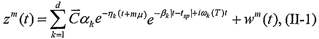
C accounts for the effect of this filter on the NQR modes. Whilst this operation will remove any known noise colouring, unknown colouring due to external RFI will still typically be present and therefore wm (t) denotes a coloured noise term. - In the following, (·) T , (·)*, (·)*, ∥·∥2 and Re{·} denote the transpose, the Hermitian transpose, the Moore-Penrose pseudoinverse, the two-norm and the real operator, respectively.
- Using (11-1), the mth echo may be written as


θ = [T βT ηT ] T , where β and η denote the vectors of unknown sinusoidal and echo dampings, respectively. Using (2), the data model for the entire echo train may then be written as

- Here, the coloured noise term,


- Since the interference subspace will typically be unknown, it must be estimated from SOI-free data.


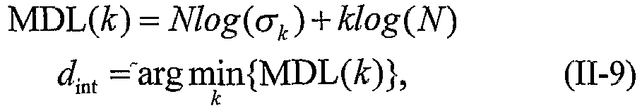
θ T αT φT ] T is given by
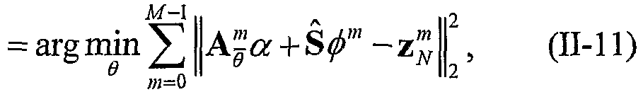
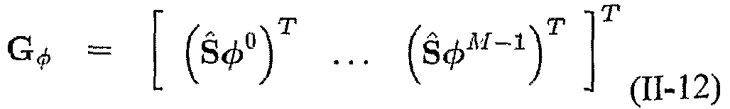
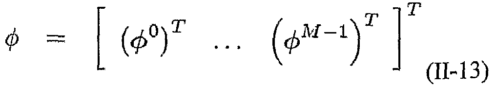
- Minimizing (II-11) with respect to φm yields an estimate of φm as

- Substituting (11-14) into (11-11) yields the compressed minimization
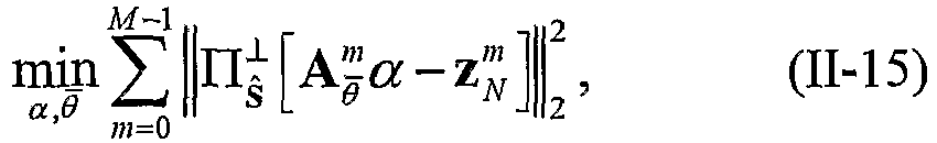
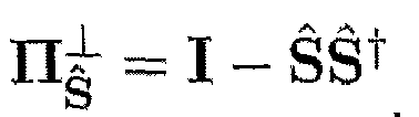
- To exploit the prior knowledge typically available for the complex amplitudes, α = ρκ is first factorized, where ρ is the common (real-valued) magnitude scaling due to the signal power, and κ is the (complex) amplitude vector, normalized such that its largest magnitude equals unity. This is further discussed in Paper B. The case when the assumed (normalized) amplitude vector, here denoted
κ is considered, as well as the actual (normalized) amplitude vector,κ , belong to an uncertainty hypersphere with radius

- The choice of ε should reflect the uncertainty in the complex amplitudes, typically obtained as a result of the experimental setup. This is further discussed in Paper B. By restricting the actual (normalized) amplitude vector to this hypersphere, an estimate of the vector best fitting the observed data can be obtained by solving the following constrained minimization

θ is here assumed known and where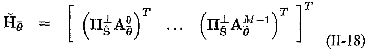

- It is noted that an initial estimate of ρ is needed to solve (17). By noting that ρ is the largest magnitude in α, an initial estimate of ρ may be obtained as ρ̂ =max {|α̂LS |} with max{x} denoting the maximum element in the vector x, and where

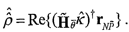

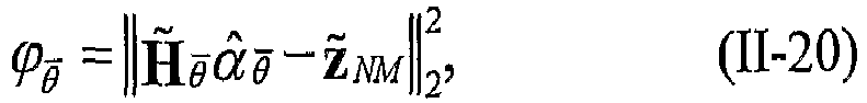
θ has been used to stress the dependence of α̂ onθ . In general,θ will be unknown and must be estimated by minimizing ϕθ overθ , using a grid search. Thus, for each value ofθ , the residual error, ϕθ , is evaluated using (II-17)-(II-20). The estimated value ofθ is then found as the parameter vector minimizing this error, i.e.,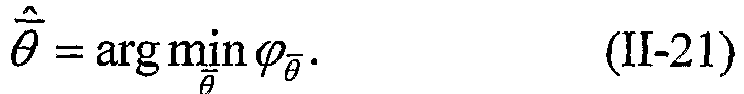
- The test statistic is formed as an approximate generalized likelihood ratio (GLRT) detector, i.e.,

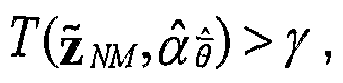
- An algorithm reminiscent of the RCDAML algorithm can also easily be derived, in which the SOI-free samples are used to form an estimate of the noise covariance matrix, from which a prewhitening transform may be obtained to reduce the effects of RFI. The results of this algorithm are here denoted the Robust Time Domain Approximate Maximum Likelihood (RTDAML) detector. Similar to SEAQUER and RCDAML, c-SEAQUER and RTDAML have a constant false alarm rate (CFAR) with respect to the additive white noise and are approximately CFAR with respect to the interference power.
-
Figure 11 shows the probability of detection as a function of the ISR, for pf = 0.05, using simulated data with SNR = -27 dB. -
Figure 12 shows the probability of detection as a function of the uncertainty parameter, v, for pf = 0.02, using simulated data with SNR = -27 dB and ISR = 60dB. -
Figure 13 shows the probability of detection as a function of
- Here, the performances of the proposed detectors are compared against current state-of-the-art detectors, namely the Robust Echo Train Approximate Maximum Likelihood (RETAML) and Frequency selective RETAML (FRETAML) algorithms, using simulated TNT data. This is further discussed in Paper B. RFI components are also added to the simulated data. Specifically, a variety of speech and audio signals are taked, sampled at 8 kHz (as for AM radio transmissions), and modulate the signals onto a carrier whose frequency is uniformly distributed over the interval [-π/4, π/4] (which corresponds to the RFI always being within 25 kHz of the excitation frequency). The resulting signal is then upsampled, according to the NQR sampling rate of 200 kHz, and added to the simulated NQR signal. The interference-to-(noise-free) NQR signal ratio (ISR) is here defined as


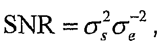

Figure 11 illustrates the probability of detection (pd ) vs the ISR, illustrating how the proposed algorithms are able to counter the RFI. The robustness to complex amplitude uncertainty is examined. Assuming a substantial interference of 60 dB, the c-SEAQUER detector is focused on, comparing it to two special cases, the c-SEAQUER-LS detector, which treats the complex amplitudes as unknown parameters, and the c-SEAQUER-ε0 detector, which exploits the relative complex amplitudes as known and without error. This is further discussed in Paper B.Figure 12 shows pd vs the uncertainty parameter, v, illustrating that the robust part of c-SEAQUER is unaffected by the presence of RFI. Similar results are obtained for RTDAML. Finally, the effect of varying
Figure 13 illustrates pd vs
- In this embodiment, a technique is provided allowing for RFI in single-sensor cNQR measurements. For the first time, we have proposed acquiring SOI-free samples, containing only corrupting signals. These samples are exploited, forming the c-SEAQUER and RTDAML detectors, both of which are able to efficiently reduce the effects of RFI. Furthermore, the performances of these algorithms on realistic cNQR signals corrupted by typical AM RFI signals are evaluated.
- In another embodiment, a representation of the corrupting signals, as modelled from noise characteristics determined from the SOI-free sample, can be simply subtracted in the frequency domain from the response signal.
- It will be understood that the present invention has been described above purely by way of example, and modifications of detail can be made within the scope of the invention as defined by the appended claims.
- Each feature disclosed in the description, and (where appropriate) the claims and drawings may be provided independently or in any appropriate combination, provided it is covered by the appended claims.
Claims (13)
- A method of testing for the presence of a species within a sample comprising the steps of:applying a spectroscopic resonance inducing excitation to the sample, wherein the excitation is a stochastic excitation, such as a random or pseudo-random excitation;detecting a resonance response signal from the sample by taking multiple samples between consecutive excitation pulses, the resonance response signal comprising a signal-of-interest of the species and at least one corrupting signal comprising radio frequency interference emanating externally to the excitation of the sample;cross-correlating the spectroscopic resonance inducing signal with the response signal to produce a correlation domain signal;processing a first part of the response signal comprising a signal-of-interest and a said corrupting signal and a second part of the response signal comprising solely a said corrupting signal, the corrupting signal being of the same type in the first and second parts; anddetermining, from the second part of the response signal, information regarding the at least one corrupting signal, and using the information to form a model of the corrupting signal;projecting the model of the corrupting signal onto the first part of the response signal to null the effects of the corrupting signal in the first part of the response signal;and then using the correlation domain signal, to derive a detector configured to determine the presence of the signal-of-interest from the first part of the response signal, when a predetermined threshold is exceeded.
- A method according to claim 1, wherein the applied excitation is a radio-frequency excitation preferably exciting in the sample one of:a nuclear quadrupole resonance;a nuclear magnetic resonance; oran electron paramagnetic resonance.
- A method according to claim 1, wherein the resulting correlation-domain signal is modelled as a gapped free-induction decay; and
preferably wherein algorithms are used to estimate spectral parameters directly from the resulting correlation-domain signal. - A method according to claim 1 or 2, wherein the corrupting signal is modelled as belonging to a low-rank linear interference subspace, embedded in wideband noise.
- A method according to claim 4, wherein the second part of the response signal is used to make an estimate of the low-rank linear interference subspace; and
preferably wherein vectors representing the response signal and the model of the corrupting signal are projected onto the space orthogonal to the interference subspace and thereby to reduce the influence of the corrupting signal in the part of the response signal containing the signal-of-interest. - A method according to any preceding claim, wherein the corrupting signal is modelled as pure zero mean Gaussian noise, and
preferably wherein the second part of the response signal is used to estimate a corresponding noise covariance matrix and to construct a transform to pre-whiten any unknown noise colouring due to the corruptive signal and thereby to reduce the influence of the corruptive signal in the first part of the response signal containing the signal-of-interest. - A method according to any preceding claim wherein the applied excitation is a radio-frequency excitation preferably exciting in the sample a nuclear quadrupole resonance, and wherein the method is used to distinguish between real and counterfeit medicines, preferably using only a single preferably non-gradiometric sensor.
- Apparatus for testing for the presence of a species within a sample comprising:means for applying a spectroscopic resonance inducing excitation to the sample, wherein the excitation signal is a stochastic signal, such as a random or pseudo-random signal;means arranged to detect a resonance response signal from the sample comprising a signal-of-interest of the species and at least one corrupting signal comprising radio frequency interference, emanating externally to the excitation of the sample;means arranged to cross-correlate the spectroscopic resonance inducing signal with the response signal to produce a correlation domain response signal;means for processing, arranged to process a first part of the response signal comprising a signal-of-interest and a corrupting signal and a second part of the response signal comprising solely a corrupting signal being of the same type in the first and second parts; andmeans arranged to determine from the second part of the response signal information regarding the at least one corrupting signal so as to model the corrupting signal, and means for using the signal information to form a model of the corrupting signal; andmeans arranged to project the model onto the first part of the response signal to null the effects of the corrupting signal in the first part of the response signal andmeans configured to use the correlation domain signal to determine the presence of the signal-of-interest from the first part of the response signal, when a predetermined threshold is exceeded.
- Apparatus according to claim 8, wherein the means for applying an excitation is adapted to apply a radio-frequency excitation, the excitation preferably exciting in the sample one of:a nuclear quadrupole resonance;a nuclear magnetic resonance; oran electron paramagnetic resonance.
- Apparatus according to claim 8 or 9, wherein the means for applying an excitation is adapted to apply a conventional pulse-sequence excitation.
- Apparatus according to claim 8 or 9, wherein
the means for processing is adapted to model the resulting correlation-domain signal as a gapped free-induction decay; and
preferably further comprising estimation means arranged to apply algorithms to estimate spectral parameters directly from the resulting correlation-domain signal. - Apparatus according to claim 11, wherein the means for processing is adapted to model the corrupting signal as belonging to a low-rank linear interference subspace, embedded in wideband noise; andpreferably wherein the means for processing is adapted to use the second part of the response signal to make an estimate of the low-rank linear interference subspace; andpreferably wherein the means for processing is adapted to project vectors representing the response signal and the model of the corrupting signal onto the space orthogonal to the interference subspace to reduce the influence of the corrupting signal in the part of the response signal containing the signal of interest.
- Apparatus according to claim 11, wherein the means for processing is further adapted to model the corrupting signal as pure zero Gaussian noise;
preferably wherein the means for processing is further adapted to use the second part of the response signal is to estimate the corresponding noise covariance matrix and to construct a pre-whitening transform for use in reducing the influence of the corruptive signal in the part of the response signal containing the signal-of-interest.
Applications Claiming Priority (2)
| Application Number | Priority Date | Filing Date | Title |
|---|---|---|---|
| GBGB0805688.9A GB0805688D0 (en) | 2008-03-28 | 2008-03-28 | Enhancing signals |
| PCT/GB2009/000803 WO2009118530A1 (en) | 2008-03-28 | 2009-03-27 | Enhancing signals |
Publications (2)
| Publication Number | Publication Date |
|---|---|
| EP2274635A1 EP2274635A1 (en) | 2011-01-19 |
| EP2274635B1 true EP2274635B1 (en) | 2020-10-21 |
Family
ID=39386936
Family Applications (1)
| Application Number | Title | Priority Date | Filing Date |
|---|---|---|---|
| EP09725323.1A Not-in-force EP2274635B1 (en) | 2008-03-28 | 2009-03-27 | Enhancing signals |
Country Status (4)
| Country | Link |
|---|---|
| US (1) | US8618798B2 (en) |
| EP (1) | EP2274635B1 (en) |
| GB (1) | GB0805688D0 (en) |
| WO (1) | WO2009118530A1 (en) |
Families Citing this family (5)
| Publication number | Priority date | Publication date | Assignee | Title |
|---|---|---|---|---|
| US9009039B2 (en) * | 2009-06-12 | 2015-04-14 | Microsoft Technology Licensing, Llc | Noise adaptive training for speech recognition |
| US8970217B1 (en) | 2010-04-14 | 2015-03-03 | Hypres, Inc. | System and method for noise reduction in magnetic resonance imaging |
| US8892140B2 (en) * | 2012-09-04 | 2014-11-18 | Futurewei Technologies, Inc. | Bi-directional training in dual networks system |
| US9575147B2 (en) | 2012-09-07 | 2017-02-21 | Morpho Detection, Llc | Nuclear quadrupole resonance system and method of using the same to remove interference components from sensor signals |
| GB2590492A (en) * | 2019-12-20 | 2021-06-30 | Henric Ryden | A method and controller for magnetic resonance imaging |
Family Cites Families (4)
| Publication number | Priority date | Publication date | Assignee | Title |
|---|---|---|---|---|
| EP0871895B1 (en) | 1995-02-24 | 2008-10-08 | QRSciences Pty. Limited | Method of and apparatus for nuclear quadrupole resonance testing a sample |
| US6121774A (en) * | 1998-06-22 | 2000-09-19 | Schlumberger Technology Corporation | Method for eliminating ringing during a nuclear magnetic resonance measurement |
| US8220334B2 (en) * | 2006-11-10 | 2012-07-17 | Penrith Corporation | Transducer array imaging system |
| US8312771B2 (en) * | 2006-11-10 | 2012-11-20 | Siemens Medical Solutions Usa, Inc. | Transducer array imaging system |
-
2008
- 2008-03-28 GB GBGB0805688.9A patent/GB0805688D0/en not_active Ceased
-
2009
- 2009-03-27 WO PCT/GB2009/000803 patent/WO2009118530A1/en not_active Ceased
- 2009-03-27 US US12/935,202 patent/US8618798B2/en not_active Expired - Fee Related
- 2009-03-27 EP EP09725323.1A patent/EP2274635B1/en not_active Not-in-force
Non-Patent Citations (1)
| Title |
|---|
| None * |
Also Published As
| Publication number | Publication date |
|---|---|
| WO2009118530A1 (en) | 2009-10-01 |
| GB0805688D0 (en) | 2008-04-30 |
| US20110210728A1 (en) | 2011-09-01 |
| US8618798B2 (en) | 2013-12-31 |
| EP2274635A1 (en) | 2011-01-19 |
Similar Documents
| Publication | Publication Date | Title |
|---|---|---|
| US11543477B2 (en) | Magnetic resonance detection (MRD) system for and methods of detecting and classifying multiple chemical substances | |
| US20020153891A1 (en) | Methods of and apparatus for analysing a signal | |
| US6420872B1 (en) | Probe for detecting a transient magnetic resonance signal, wherein the ratio of the Q of the probe to the Q of the resonance signal is relatively large | |
| WO2003076952A2 (en) | Three-frequency nuclear quadrupole resonance (nqr) | |
| EP2274635B1 (en) | Enhancing signals | |
| Somasundaram et al. | Exploiting spin echo decay in the detection of nuclear quadrupole resonance signals | |
| Mozzhukhin et al. | The detection of industrial explosives by the quadrupole resonance method: some aspects of the detection of ammonium nitrate and trinitrotoluene | |
| Shao et al. | Detecting NQR signals severely polluted by interference | |
| Monea | Signal processing and analysis methods in nuclear quadrupole resonance spectroscopy | |
| WO2002044747A1 (en) | Decoupling sideband resolved nmr spectroscopy (desire) | |
| Monea et al. | An optimized NQR spectrometer for detection of prohibited substances | |
| Somasundaram et al. | Robust detection of stochastic nuclear quadrupole resonance signals | |
| Mandal et al. | Two-dimensional NQR using ultra-broadband electronics | |
| Somasundaram et al. | Countering radio frequency interference in single-sensor quadrupole resonance | |
| Somasundaram et al. | Robust nuclear quadrupole resonance signal detection allowing for amplitude uncertainties | |
| Hemnani et al. | 14 N NQR spectrometer for explosive detection: A review | |
| Mozzhukhin et al. | Three-frequency composite multipulse nuclear quadrupole resonance technique for explosive detection | |
| Somasundaram et al. | Analysis of nuclear quadrupole resonance signals from mixtures | |
| US7791342B2 (en) | Cancellation of ringing artifacts and far field interference in nuclear quadrupole resonance | |
| Zhu et al. | Nuclear quadrupole resonance signal detectability enhancement methods—An overview | |
| Jakobsson et al. | Using spatial diversity to detect narcotics and explosives using NQR signals | |
| Shan | EMD and wavelet methods for interference cancellation in quadrupole resonance detection | |
| Tseytlin et al. | Decoupling of excitation and receive coils in pulsed magnetic resonance using sinusoidal magnetic field modulation | |
| Mozzhukhin et al. | Two-frequency nuclear quadrupole resonance for line identification | |
| Mozzhukhin et al. | Sensing system for 14 N NQR remote detection of explosives |
Legal Events
| Date | Code | Title | Description |
|---|---|---|---|
| PUAI | Public reference made under article 153(3) epc to a published international application that has entered the european phase |
Free format text: ORIGINAL CODE: 0009012 |
|
| 17P | Request for examination filed |
Effective date: 20101028 |
|
| AK | Designated contracting states |
Kind code of ref document: A1 Designated state(s): AT BE BG CH CY CZ DE DK EE ES FI FR GB GR HR HU IE IS IT LI LT LU LV MC MK MT NL NO PL PT RO SE SI SK TR |
|
| AX | Request for extension of the european patent |
Extension state: AL BA RS |
|
| DAX | Request for extension of the european patent (deleted) | ||
| 17Q | First examination report despatched |
Effective date: 20150921 |
|
| STAA | Information on the status of an ep patent application or granted ep patent |
Free format text: STATUS: EXAMINATION IS IN PROGRESS |
|
| GRAP | Despatch of communication of intention to grant a patent |
Free format text: ORIGINAL CODE: EPIDOSNIGR1 |
|
| STAA | Information on the status of an ep patent application or granted ep patent |
Free format text: STATUS: GRANT OF PATENT IS INTENDED |
|
| INTG | Intention to grant announced |
Effective date: 20200511 |
|
| GRAS | Grant fee paid |
Free format text: ORIGINAL CODE: EPIDOSNIGR3 |
|
| GRAA | (expected) grant |
Free format text: ORIGINAL CODE: 0009210 |
|
| STAA | Information on the status of an ep patent application or granted ep patent |
Free format text: STATUS: THE PATENT HAS BEEN GRANTED |
|
| AK | Designated contracting states |
Kind code of ref document: B1 Designated state(s): AT BE BG CH CY CZ DE DK EE ES FI FR GB GR HR HU IE IS IT LI LT LU LV MC MK MT NL NO PL PT RO SE SI SK TR |
|
| REG | Reference to a national code |
Ref country code: GB Ref legal event code: FG4D |
|
| REG | Reference to a national code |
Ref country code: CH Ref legal event code: EP |
|
| REG | Reference to a national code |
Ref country code: IE Ref legal event code: FG4D |
|
| REG | Reference to a national code |
Ref country code: DE Ref legal event code: R096 Ref document number: 602009062940 Country of ref document: DE |
|
| REG | Reference to a national code |
Ref country code: AT Ref legal event code: REF Ref document number: 1326348 Country of ref document: AT Kind code of ref document: T Effective date: 20201115 |
|
| REG | Reference to a national code |
Ref country code: DE Ref legal event code: R082 Ref document number: 602009062940 Country of ref document: DE Representative=s name: MATHYS & SQUIRE EUROPE PATENTANWAELTE PARTNERS, DE Ref country code: DE Ref legal event code: R082 Ref document number: 602009062940 Country of ref document: DE Representative=s name: MATHYS & SQUIRE GBR, DE |
|
| REG | Reference to a national code |
Ref country code: AT Ref legal event code: MK05 Ref document number: 1326348 Country of ref document: AT Kind code of ref document: T Effective date: 20201021 |
|
| REG | Reference to a national code |
Ref country code: NL Ref legal event code: MP Effective date: 20201021 |
|
| PG25 | Lapsed in a contracting state [announced via postgrant information from national office to epo] |
Ref country code: FI Free format text: LAPSE BECAUSE OF FAILURE TO SUBMIT A TRANSLATION OF THE DESCRIPTION OR TO PAY THE FEE WITHIN THE PRESCRIBED TIME-LIMIT Effective date: 20201021 Ref country code: NL Free format text: LAPSE BECAUSE OF FAILURE TO SUBMIT A TRANSLATION OF THE DESCRIPTION OR TO PAY THE FEE WITHIN THE PRESCRIBED TIME-LIMIT Effective date: 20201021 Ref country code: NO Free format text: LAPSE BECAUSE OF FAILURE TO SUBMIT A TRANSLATION OF THE DESCRIPTION OR TO PAY THE FEE WITHIN THE PRESCRIBED TIME-LIMIT Effective date: 20210121 Ref country code: PT Free format text: LAPSE BECAUSE OF FAILURE TO SUBMIT A TRANSLATION OF THE DESCRIPTION OR TO PAY THE FEE WITHIN THE PRESCRIBED TIME-LIMIT Effective date: 20210222 Ref country code: GR Free format text: LAPSE BECAUSE OF FAILURE TO SUBMIT A TRANSLATION OF THE DESCRIPTION OR TO PAY THE FEE WITHIN THE PRESCRIBED TIME-LIMIT Effective date: 20210122 |
|
| PGFP | Annual fee paid to national office [announced via postgrant information from national office to epo] |
Ref country code: FR Payment date: 20210325 Year of fee payment: 13 |
|
| REG | Reference to a national code |
Ref country code: LT Ref legal event code: MG4D |
|
| PG25 | Lapsed in a contracting state [announced via postgrant information from national office to epo] |
Ref country code: SE Free format text: LAPSE BECAUSE OF FAILURE TO SUBMIT A TRANSLATION OF THE DESCRIPTION OR TO PAY THE FEE WITHIN THE PRESCRIBED TIME-LIMIT Effective date: 20201021 Ref country code: PL Free format text: LAPSE BECAUSE OF FAILURE TO SUBMIT A TRANSLATION OF THE DESCRIPTION OR TO PAY THE FEE WITHIN THE PRESCRIBED TIME-LIMIT Effective date: 20201021 Ref country code: LV Free format text: LAPSE BECAUSE OF FAILURE TO SUBMIT A TRANSLATION OF THE DESCRIPTION OR TO PAY THE FEE WITHIN THE PRESCRIBED TIME-LIMIT Effective date: 20201021 Ref country code: BG Free format text: LAPSE BECAUSE OF FAILURE TO SUBMIT A TRANSLATION OF THE DESCRIPTION OR TO PAY THE FEE WITHIN THE PRESCRIBED TIME-LIMIT Effective date: 20210121 Ref country code: AT Free format text: LAPSE BECAUSE OF FAILURE TO SUBMIT A TRANSLATION OF THE DESCRIPTION OR TO PAY THE FEE WITHIN THE PRESCRIBED TIME-LIMIT Effective date: 20201021 Ref country code: ES Free format text: LAPSE BECAUSE OF FAILURE TO SUBMIT A TRANSLATION OF THE DESCRIPTION OR TO PAY THE FEE WITHIN THE PRESCRIBED TIME-LIMIT Effective date: 20201021 Ref country code: IS Free format text: LAPSE BECAUSE OF FAILURE TO SUBMIT A TRANSLATION OF THE DESCRIPTION OR TO PAY THE FEE WITHIN THE PRESCRIBED TIME-LIMIT Effective date: 20210221 |
|
| PGFP | Annual fee paid to national office [announced via postgrant information from national office to epo] |
Ref country code: DE Payment date: 20210323 Year of fee payment: 13 Ref country code: GB Payment date: 20210308 Year of fee payment: 13 |
|
| PG25 | Lapsed in a contracting state [announced via postgrant information from national office to epo] |
Ref country code: HR Free format text: LAPSE BECAUSE OF FAILURE TO SUBMIT A TRANSLATION OF THE DESCRIPTION OR TO PAY THE FEE WITHIN THE PRESCRIBED TIME-LIMIT Effective date: 20201021 |
|
| REG | Reference to a national code |
Ref country code: DE Ref legal event code: R097 Ref document number: 602009062940 Country of ref document: DE |
|
| PG25 | Lapsed in a contracting state [announced via postgrant information from national office to epo] |
Ref country code: LT Free format text: LAPSE BECAUSE OF FAILURE TO SUBMIT A TRANSLATION OF THE DESCRIPTION OR TO PAY THE FEE WITHIN THE PRESCRIBED TIME-LIMIT Effective date: 20201021 Ref country code: EE Free format text: LAPSE BECAUSE OF FAILURE TO SUBMIT A TRANSLATION OF THE DESCRIPTION OR TO PAY THE FEE WITHIN THE PRESCRIBED TIME-LIMIT Effective date: 20201021 Ref country code: CZ Free format text: LAPSE BECAUSE OF FAILURE TO SUBMIT A TRANSLATION OF THE DESCRIPTION OR TO PAY THE FEE WITHIN THE PRESCRIBED TIME-LIMIT Effective date: 20201021 Ref country code: SK Free format text: LAPSE BECAUSE OF FAILURE TO SUBMIT A TRANSLATION OF THE DESCRIPTION OR TO PAY THE FEE WITHIN THE PRESCRIBED TIME-LIMIT Effective date: 20201021 Ref country code: RO Free format text: LAPSE BECAUSE OF FAILURE TO SUBMIT A TRANSLATION OF THE DESCRIPTION OR TO PAY THE FEE WITHIN THE PRESCRIBED TIME-LIMIT Effective date: 20201021 |
|
| PLBE | No opposition filed within time limit |
Free format text: ORIGINAL CODE: 0009261 |
|
| STAA | Information on the status of an ep patent application or granted ep patent |
Free format text: STATUS: NO OPPOSITION FILED WITHIN TIME LIMIT |
|
| PG25 | Lapsed in a contracting state [announced via postgrant information from national office to epo] |
Ref country code: DK Free format text: LAPSE BECAUSE OF FAILURE TO SUBMIT A TRANSLATION OF THE DESCRIPTION OR TO PAY THE FEE WITHIN THE PRESCRIBED TIME-LIMIT Effective date: 20201021 |
|
| 26N | No opposition filed |
Effective date: 20210722 |
|
| PG25 | Lapsed in a contracting state [announced via postgrant information from national office to epo] |
Ref country code: MC Free format text: LAPSE BECAUSE OF FAILURE TO SUBMIT A TRANSLATION OF THE DESCRIPTION OR TO PAY THE FEE WITHIN THE PRESCRIBED TIME-LIMIT Effective date: 20201021 Ref country code: IT Free format text: LAPSE BECAUSE OF FAILURE TO SUBMIT A TRANSLATION OF THE DESCRIPTION OR TO PAY THE FEE WITHIN THE PRESCRIBED TIME-LIMIT Effective date: 20201021 |
|
| REG | Reference to a national code |
Ref country code: CH Ref legal event code: PL |
|
| PG25 | Lapsed in a contracting state [announced via postgrant information from national office to epo] |
Ref country code: SI Free format text: LAPSE BECAUSE OF FAILURE TO SUBMIT A TRANSLATION OF THE DESCRIPTION OR TO PAY THE FEE WITHIN THE PRESCRIBED TIME-LIMIT Effective date: 20201021 |
|
| REG | Reference to a national code |
Ref country code: BE Ref legal event code: MM Effective date: 20210331 |
|
| PG25 | Lapsed in a contracting state [announced via postgrant information from national office to epo] |
Ref country code: LU Free format text: LAPSE BECAUSE OF NON-PAYMENT OF DUE FEES Effective date: 20210327 Ref country code: LI Free format text: LAPSE BECAUSE OF NON-PAYMENT OF DUE FEES Effective date: 20210331 Ref country code: CH Free format text: LAPSE BECAUSE OF NON-PAYMENT OF DUE FEES Effective date: 20210331 Ref country code: IE Free format text: LAPSE BECAUSE OF NON-PAYMENT OF DUE FEES Effective date: 20210327 |
|
| PG25 | Lapsed in a contracting state [announced via postgrant information from national office to epo] |
Ref country code: IS Free format text: LAPSE BECAUSE OF FAILURE TO SUBMIT A TRANSLATION OF THE DESCRIPTION OR TO PAY THE FEE WITHIN THE PRESCRIBED TIME-LIMIT Effective date: 20210221 |
|
| PG25 | Lapsed in a contracting state [announced via postgrant information from national office to epo] |
Ref country code: BE Free format text: LAPSE BECAUSE OF NON-PAYMENT OF DUE FEES Effective date: 20210331 |
|
| REG | Reference to a national code |
Ref country code: DE Ref legal event code: R119 Ref document number: 602009062940 Country of ref document: DE |
|
| GBPC | Gb: european patent ceased through non-payment of renewal fee |
Effective date: 20220327 |
|
| PG25 | Lapsed in a contracting state [announced via postgrant information from national office to epo] |
Ref country code: GB Free format text: LAPSE BECAUSE OF NON-PAYMENT OF DUE FEES Effective date: 20220327 Ref country code: FR Free format text: LAPSE BECAUSE OF NON-PAYMENT OF DUE FEES Effective date: 20220331 Ref country code: DE Free format text: LAPSE BECAUSE OF NON-PAYMENT OF DUE FEES Effective date: 20221001 |
|
| PG25 | Lapsed in a contracting state [announced via postgrant information from national office to epo] |
Ref country code: HU Free format text: LAPSE BECAUSE OF FAILURE TO SUBMIT A TRANSLATION OF THE DESCRIPTION OR TO PAY THE FEE WITHIN THE PRESCRIBED TIME-LIMIT; INVALID AB INITIO Effective date: 20090327 Ref country code: CY Free format text: LAPSE BECAUSE OF FAILURE TO SUBMIT A TRANSLATION OF THE DESCRIPTION OR TO PAY THE FEE WITHIN THE PRESCRIBED TIME-LIMIT Effective date: 20201021 |
|
| PG25 | Lapsed in a contracting state [announced via postgrant information from national office to epo] |
Ref country code: MK Free format text: LAPSE BECAUSE OF FAILURE TO SUBMIT A TRANSLATION OF THE DESCRIPTION OR TO PAY THE FEE WITHIN THE PRESCRIBED TIME-LIMIT Effective date: 20201021 |
|
| PG25 | Lapsed in a contracting state [announced via postgrant information from national office to epo] |
Ref country code: MT Free format text: LAPSE BECAUSE OF FAILURE TO SUBMIT A TRANSLATION OF THE DESCRIPTION OR TO PAY THE FEE WITHIN THE PRESCRIBED TIME-LIMIT Effective date: 20201021 |
|
| PG25 | Lapsed in a contracting state [announced via postgrant information from national office to epo] |
Ref country code: TR Free format text: LAPSE BECAUSE OF FAILURE TO SUBMIT A TRANSLATION OF THE DESCRIPTION OR TO PAY THE FEE WITHIN THE PRESCRIBED TIME-LIMIT Effective date: 20201021 |