EP2157521A1 - Method for tire rolling simulation on mud - Google Patents
Method for tire rolling simulation on mud Download PDFInfo
- Publication number
- EP2157521A1 EP2157521A1 EP09006542A EP09006542A EP2157521A1 EP 2157521 A1 EP2157521 A1 EP 2157521A1 EP 09006542 A EP09006542 A EP 09006542A EP 09006542 A EP09006542 A EP 09006542A EP 2157521 A1 EP2157521 A1 EP 2157521A1
- Authority
- EP
- European Patent Office
- Prior art keywords
- stress
- mud
- tire
- strain
- model
- Prior art date
- Legal status (The legal status is an assumption and is not a legal conclusion. Google has not performed a legal analysis and makes no representation as to the accuracy of the status listed.)
- Withdrawn
Links
Images





Classifications
-
- G—PHYSICS
- G06—COMPUTING OR CALCULATING; COUNTING
- G06F—ELECTRIC DIGITAL DATA PROCESSING
- G06F9/00—Arrangements for program control, e.g. control units
- G06F9/06—Arrangements for program control, e.g. control units using stored programs, i.e. using an internal store of processing equipment to receive or retain programs
- G06F9/44—Arrangements for executing specific programs
- G06F9/455—Emulation; Interpretation; Software simulation, e.g. virtualisation or emulation of application or operating system execution engines
-
- B—PERFORMING OPERATIONS; TRANSPORTING
- B60—VEHICLES IN GENERAL
- B60C—VEHICLE TYRES; TYRE INFLATION; TYRE CHANGING; CONNECTING VALVES TO INFLATABLE ELASTIC BODIES IN GENERAL; DEVICES OR ARRANGEMENTS RELATED TO TYRES
- B60C99/00—Subject matter not provided for in other groups of this subclass
- B60C99/006—Computer aided tyre design or simulation
-
- G—PHYSICS
- G01—MEASURING; TESTING
- G01M—TESTING STATIC OR DYNAMIC BALANCE OF MACHINES OR STRUCTURES; TESTING OF STRUCTURES OR APPARATUS, NOT OTHERWISE PROVIDED FOR
- G01M17/00—Testing of vehicles
- G01M17/007—Wheeled or endless-tracked vehicles
- G01M17/02—Tyres
-
- G—PHYSICS
- G06—COMPUTING OR CALCULATING; COUNTING
- G06F—ELECTRIC DIGITAL DATA PROCESSING
- G06F30/00—Computer-aided design [CAD]
- G06F30/10—Geometric CAD
- G06F30/15—Vehicle, aircraft or watercraft design
-
- G—PHYSICS
- G06—COMPUTING OR CALCULATING; COUNTING
- G06F—ELECTRIC DIGITAL DATA PROCESSING
- G06F30/00—Computer-aided design [CAD]
- G06F30/20—Design optimisation, verification or simulation
- G06F30/23—Design optimisation, verification or simulation using finite element methods [FEM] or finite difference methods [FDM]
Definitions
- the present invention relates to a method for tire rolling simulation capable of predicting a tire performance on mud.
- a method for tire rolling simulation on mud comprises the steps of modeling a tire using finite elements to build a tire model, modeling a muddy road covered with mud using finite volumes to build a muddy road model which can exhibit elastoplasticity property, and failure property in which the finite volume fails under a certain tensile stress, but does not fail under any compression stress, and executing a numerical simulation in which the tire model is made to roll on the muddy road model in a predetermined condition.
- the simulation method of this embodiment is to roll a tire model 2 on a road covered with thick mud layer.
- mud comprises a mixture of mud particles of at least one kind of: clay having a particle size of less than 0.005 mm; silt having a particle size of from 0.005 to 0.075 mm; fine mud having a particle size of from 0.075 to 0.250 mm; medium mud having a particle size of from 0.250 to 0.850 mm; fine gravel having a particle size of from 0.850 to 2.00 mm; granule having a particle size of from 2.00 to 4.75 mm; or medium gravel having a particle size of from 4.75 to 19.00 mm.
- the particle size is preferably not more than 9.50 mm, and percentage of water content is preferably set in the range of from 10 to 50%, more preferably in the range of from 10 to 40%.
- Fig. 1 shows a computer device 1 used for the simulation method of the present invention.
- the computer device 1 comprises a main body 1a, a keyboard 1b, a mouse 1c, and a display device 1d.
- the main body 1a includes disk drives 1a1 and 1a2, a CPU, a ROM, a memory, and a bulk storage (which are not illustrated).
- the bulk storage stores programs, which execute the simulation method described below.
- Fig. 2 shows an example of the procedure of the invention simulation method.
- a tire model 2 is set by modeling a tire using finite elements capable of numerical analysis.
- the numerical analysis includes, for example, the finite element method, the finite volume method, the finite difference method and the boundary element method.
- the finite element method and the finite volume method are employed.
- Fig. 3 is an example of the tire model 2 which is visualized in three-dimensional.
- the tire to be analyzed is divided into a finite number of small elements (LaGrange elements) 2a, 2b, 2c which are numerical data capable of calculation by the computer device 1.
- the tire model 2 includes the coordinate values of the nodal points of each element 2a, 2b, 2c ..., their nodal numbers, and their properties such as density, Young's modulus, damping coefficient.
- Each of the elements 2a, 2b, 2c ... can be, but not limited to, rectangular plane elements or three-dimensional tetrahedral solid elements. Other various elements such as pentagonal and/or hexagonal solid elements are also employed.
- the tire model 2 shown in Fig. 3 is provided with tread grooves on the tread including longitudinal and transverse grooves, but these may be omitted.
- the circumferential length of one element arranged on the tread of the tire model 2 does not preferably exceed 25% of a circumferential length of the tread ground contact portion. This is useful for correct expression of the tread ground contact pressure or the distribution of the shearing force.
- the length of one element in the axial direction of the tire is preferably 20 mm or less.
- the tire model 2 could be, but not limited to, a combination of the detailed pattern part "A” that has modeled grooves on the tread and the simple pattern part B that has no grooves on the tread.
- the detailed pattern part "A” is longer than the tread ground contact portion in the tire circumferential direction, but is shorter than the simple pattern part B. This helps to accelerate the calculation time by reducing the number of elements in the tire model 2 as a whole.
- Fig. 5 shows an example of modeling of a cord reinforcement member c such as a belt ply, a carcass ply or the like.
- the cord reinforcement members c are modeled into membrane elements 5a and 5b, and the topping rubber part t is modeled into solid elements 5c, 5d and 5e. These elements are stacked in the direction of a thickness so as to form a shell element 5.
- the membrane elements 5a and 5b have anisotropy that is different stiffness in the longitudinal direction of the cord c1 and the direction orthogonal thereto. Further, a viscoelastic property is defined in the solid elements.
- a muddy road model is set by modeling muddy road in finite volumes capable of the numerical analysis above.
- the muddy road model is modeled in this embodiment using Euler finite volumes.
- Fig. 6 shows an example of the muddy road model 6.
- the muddy road model 6 comprises: a three-dimensional regular finite volume mesh 6a fixed on the stiff element 7; and the numerical mud material 6c corresponding to the mud packed in the spaces 6b divided by the mesh 6a.
- the mud material 6c can move in the space 6b of the mesh 6a having a bottom and sidewalls.
- the thickness H of the mud material 6c corresponds to the thickness of the mud layer to be evaluated. In this embodiment, the thickness is taken large enough to represent deep mud.
- the term "one volume of the muddy road model" means one hexagonal space 6b and the numerical mud material 6c therein.
- the muddy road model 6 has a width and a length as necessary for the rotation of the tire model 2.
- Figs. 7(a) and 7 ((b) show a state in which the muddy road model 6 gets into contact with the tire model 2.
- the crossing portion J between the tire model 2 and the numerical mud material 6c is calculated based on mutual position information. Then, the tire model 2 and the mud material 6c are coupled at the boundary JL of the crossing portion J so as to interact with each other. Namely, the mud material 6c provides reaction force to the tire model 2 through the boundary JL.
- the tire model 2 provides the mud material 6c with a moving boundary surface (coupling surface). Therefore, mud material 6c in the cross portion J is moved out of the model so that the mud material 6c is compressed along the tread of the tire model.
- elastoplasticity property, failure property, and adhesion are defined in the mud material 6c.
- the elastoplasticity is a state of a substance subjected to a stress greater than its elastic limit but not so great as to cause it to rupture, in which it exhibits both elastic and plastic properties.
- the numerical mud material 6c can change its physical property according to its state of the stress.
- the inventors have found that the behavior of mud with, but not limited to, a particle size can be represented by elastoplasticity. That is, the mud hasviscosity, so that the deformation property thereof is dependent on the strain rate.
- the elastoplasticity is preferably to be set according to mud properties that are to be evaluated for the target mud.
- the elastoplasticity of the mud is determined based on results of the triaxial compression tests in which the mud is compressed with an axial force under an external pressure that is kept constant.
- the failure property is denoted as the following characteristics: the mud material 6c does not fail by compression stress (average compression stress) even if plastic strain occurs therein; and the mud material 6c fails by tensile stress (average tensile stress) when equivalent plastic strain reaches a particular value.
- the equivalent plastic strain is kept constant regardless of the external pressure.
- the failure property is also preferably to be set according to mud properties that are to be evaluated for the target mud.
- the failure property of the mud is determined based on results of the hollow cylinder tensile tests.
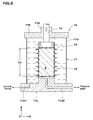
- Fig. 8 schematically shows an example of a compression test machine 10 for mud.
- the compression test machine 10 comprises: a pressure chamber 11 filled with a liquid such as water; a cylindrical container 12 packed with mud S and placed inside the chamber 11; and an actuator 14 which can apply an axial compressive force on the container 12 and the mud inside.
- the pressure chamber 11 comprises: a cylindrical main body 11a having a space therein; an upper cover 11b to close a top of the main body 11a with a guide 11d for the piston rod of the actuator 14; and a bottom cover 11c to close the bottom of the main body 11a.
- the internal pressure of the chamber 11 is kept constant by controlling amount of the liquid using a control device (not shown).
- the bottom cover 11c is provided with a passage 11e1 connecting the bottom of the container 12 to the control device and a second passage 11e2 connected to a pressure gage (not shown).
- the cylindrical container 12 has a thin and soft sidewall made of rubber or the like such that it does not have substantial stiffness.
- the container 12 has a diameter of about 5cm.
- test mud s is tightly packed in the container 12. Therefore, the mud s receives pressure from the liquid in the chamber 11 through the soft sidewall of the container 12. Further, the bottom of the container 12 is fixed on the lower cover 11c, and its top is pushed by the piston rod of the actuator 14. Also, the sidewall of the container 12 receives liquid pressure in the chamber 11.
- the liquid pressure in the chamber 11 is defined as external pressure for the mud S.
- the compression test is performed under at least two, or preferably three different levels of external pressure acting on mud. Further, the levels of external pressure are preferably determined in consideration of the contact pressure of the tire. In this embodiment, the mud compression tests have been performed under three levels of external pressure of 98 kPa, 196 kPa, and 294 kPa, respectively.
- the mud s filled in the container 12 is in a triaxial stress state receiving external pressure in x, Y, and z directions and compressive axial force in z direction from the actuator 14.
- the actuator 14 under a constant external pressure, when increasing the axial force, particles of the mud begin to slip, and then the container 12 bulges in its radial direction.
- the relationship between the axial stress and the axial plastic compression strain of the mud is obtained from the result of these compression tests.
- the actuator 14 is pressed down by the velocities ⁇ '1 and ⁇ '2 (> ⁇ '1) under each of the three leveled external pressures to reflect strain velocity in the simulation.
- ⁇ a ⁇ L / L ⁇ 0
- Fig. 9 shows that the relationship between the axial plastic compression strain ⁇ a and the deviatoric stress ( ⁇ a- ⁇ r) of the mud s varies according to the external pressure. That is, when the compression velocity is higher, the deviatonic stress is also higher. The strain rate dependency appears prominently.
- the stress-strain relationship namely the elastoplasticity, under three different levels of external pressures and two different levels of strain velocities as obtained in the compression tests, is defined as the elastic-plastic relationship of the muddy road model 6.
- each finite volume of the muddy road model 6 behaves according to the relationship shown in Fig. 9 .
- the computer device 1 depicts these curves shown in Fig. 9 as functions and/or approximate curves and stores them.
- the stress-strain relationship excepting under each of the above mentioned predetermined levels of external pressures and strain velocities can be obtained by interpolation.
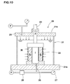
- Fig. 10 shows an embodiment of a tensile test machine 20 for hollow cylinder tensile tests to study the failure property of mud.
- the tensile test machine 20, as well as the triaxial compression tests machine 10, comprises:
- the container 22 has a thin and soft sidewall made of rubber or the like such that it does not have substantial stiffness.
- the pressure chamber 21 comprises: an upper cover 21a and a bottom cover 21b.
- the upper cover 21a having a flow channel 25 to inflate high-pressure air from a pressure pump P so as to the outer surfaces of the container 22 can be applied a pressure Po through the liquid W.
- the bottom cover 21b having a flow channel 26 to inflate high-pressure air from a pressure pump P into the hollow (i) so as to apply arbitrary pressure Pi on the surface of the mud S from the side of the hollow (i).
- the actions of the tensile test machine 20 are described below.
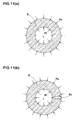
- certain pressures Pi and Po were applied into the pressure chamber 21 and the hollow (i) of container 22, respectively.
- the actuator 23 presses the container 22 so that the compression pressure applied to the container 22 is as much as the external pressure Po.
- the pressure Po of the pressure chamber 22 While keeping the pressure Po of the pressure chamber 22 constant, the pressure Pi in the hollow (i) of the container 22 is increased until cracks Sc occurring in the mud s of the container 22 as shown in Fig. 11(b) .
- the pressure P of the actuator 23 is supplemented with the pressure increasing in the hollow (i).
- a manometer 27 and a flow meter 28 measure the internal pressure Pi and volume increases of the container 22, respectively.
- the hollow cylinder tensile tests have been performed under two levels of external pressure Po of 19.6 kPa and 98.0 kPa.
- Mud is unfit for a conventional tensile test.
- the present embodiment allows to test its failure property.
- the mud is contained in the ring-shaped hollow cylindrical container 22; the hollow (i) thereof is applied pressure; and the mud is applied the tensile stress in the circumferential direction until failing.
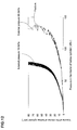
- Fig. 12 shows the results of the above-described hollow cylinder tensile tests.
- the volume of the hollow (i) gradually increases in accordance with the increase of the inner pressure Pi initially. Then, the inner pressure Pi hardly increases, however, the volume of the hollow (i) suddenly increases, and finally yields and then fails. Meanwhile, the failure strain does not depend on the external pressure but is constant. In the present embodiment, the failure strain is stored in the computer device 1.
- mud has strong adhesion.
- the volume of the mud model 6 gets out when the equivalent plastic strain thereof is over the certain value predetermined based on the failure property under tensile stress condition, so that it is useful in simulating accurately the representation of rolling resistance caused by mud.
- Adhesion frictional force between the tire surface and the mud occurs also in the tensile stress condition. The adhesion force and adhesion frictional force are predetermined between the tire model 2 and muddy road model 6, and these forces are considered in the deformation calculation for simulation.
- Fig. 13(a) shows a schematic illustration wherein the tire model 2 and the muddy road model 6 are in compression.
- vertical reactive force N and frictional force ⁇ N that is caused by locomotion ( ⁇ : coefficient of dynamic friction) arise. These forces affect on the tire model 2.
- adhersion frictional force adhesive force and frictional force that is caused by locomotion
- the adhesive force is normal force, arises ongoingly, and continues to increase to the break point of the mud material 6c of the muddy road model 6. Moreover, the adhesive force is set to be particularly larger than the breaking strength of the muddy road model 6.
- the adhesion frictional force is a force perpendicular to the above-mentioned adhesive force, and continues to generate until it reaches maximum frictional force.
- the simulation with this generation of frictional force under the tensile stress condition, in view of the adhesive force can represent more accurately the condition of tire rolling in muddy road.
- boundary conditions for the simulation are set.
- the boundary conditions include wheel rims, internal pressure of the tire model 2, friction coefficient between the tire model 2 and the muddy road model 6, the tire load, the slip angle, the camber angle, rotating speed (In this embodiment, rotational and translational speeds are set to the tire model 2.), initial time increment for deformation calculation of each model and initial position of each model 2 and 6.
- Fig. 14 shows the virtual rim assembly of the tire model 2.
- a pair of bead regions 2r of the tire model 2 are equal to the rim width.
- the radial distance (r) from the rotation axis CL of the tire model 2 to the bead regions 2r is set to be equal to the rim diameter.
- the internal pressure is expressed by applying an uniformly distributed load (w) having the same value as the internal pressure of the tire on the internal surface of the tire model 2.
- the explicit time integration method is employed in the simulation in this present example.
- the moment that the load acts on each model is taken as time zero, and the time is divided into small increments so as to find the displacement of the model at each point in time.
- the explicit method does not involve convergence calculations. However, it is necessary that the time increment satisfies the "Courant criterion", in order to stabilize the calculations.
- the initial time increment ⁇ t in the deformation calculation for the tire model 2 and the muddy road model 6 is set at the values that meet the following formula (1). ⁇ t ⁇ L min / C
- L min is the characteristic length of the smallest element in each model
- the propagating time of the stress wave of each element is calculated based on the formula (1), and after that, the time increment is set up by multiplying the minimum of the propagating time by a safety factor.
- the safety factor is, for example, more preferably set equal to 0.66.
- the initial time increment is preferably set of from 0.1 to 5 ⁇ sec, more preferably 0.3 to 3 ⁇ sec, and most preferably 0.5 to 2 ⁇ sec for both the tire model 2 and the muddy road model 6.
- the deformation calculation of the tire model 2 and the deformation calculation of the muddy road model 6 are performed separately.
- the position, the shape and the speed data of the tire model 2 obtained from the deformation calculation of the tire model 2 are given to the muddy road model 6 as a boundary condition for the deformation calculation of the muddy road model 6 (Step S8).
- the pressure and frictional force obtained from the deformation calculation of the muddy road model 6 are given to the tire model 2 as the boundary condition (load) for the deformation calculation of the tire model 2 (Step S7).
- Fig. 16 shows an example of the deformation calculation of the tire model 2.
- Step S41 shown in Fig. 16 the deformation calculation after the time increment ⁇ t is performed first.
- the deformation calculation in the present example is performed by the computer device 1 to solve equations of motion. Calculated values indicate the state that the tire rolls on the muddy road model 6 for the time increment ⁇ t.
- the stress wave propagation time of each element of the deformed tire model 2 is calculated based on its size, density and stiffness (Step S42). Then, based on the minimum value of this stress wave propagation time, the time increment for the next deformation calculation is set so as to satisfy the Courant criterion above (Step S43). Since the stress wave propagation time is a function of the size and density of the element, it changes every time the element deforms. In the present embodiment, the optimum time increment is set in accordance with the deformation of the element, which helps the deformation calculation of the tire model 2 to be performed more accurately.
- Step S44 it is checked whether the predetermined duration of simulation time has been elapsed or not (Step S44).
- Step S44 it is checked whether the predetermined duration of simulation time has been elapsed or not.
- Step S44 the process goes back to the Step S41 to perform one more calculation by adding the newly set time increment.
- Step S44 the deformation calculation of the tire model 2 is terminated and the process goes to the Step S6.
- Fig. 17 shows an example of the deformation calculation of the muddy road model 6.
- the deformation calculation of the material in each finite volume of the muddy road model 6 is performed after the time increment (Step S51).
- the density ⁇ of each finite volume of the muddy road model 6 is calculated because the density of the mud material 6c of the muddy model 6 changes in accordance with positions of the tire model 2.
- ⁇ 0 is the initial density of the finite volume under zero pressure, and the compressive volume strain is expressed as negative.
- Step S52 the stress calculation of the muddy road model 6 after the time increment is performed.
- the second invariant J 2 of the stress tensor of each finite volume of the muddy road model 6 are calculated using deviatoric stresses of each volume.
- Each of the normal deviatoric stresses ⁇ x ', ⁇ y ', and ⁇ z ' is calculated by subtracting the pressure P evaluated above from each of the normal stresses, ⁇ x , ⁇ y , and ⁇ z .
- the second invariant J 2 of the stress tensor is calculated by the following equation (8) using the above deviatoric stress and shear stress components.
- J 2 ⁇ x ⁇ ⁇ ⁇ ⁇ y ⁇ ⁇ + ⁇ y ⁇ ⁇ ⁇ ⁇ z ⁇ ⁇ + ⁇ z ⁇ ⁇ ⁇ ⁇ ⁇ x ⁇ ⁇ - ⁇ xy 2 - ⁇ yz 2 - ⁇ zx 2
- ⁇ xy , ⁇ yz , and ⁇ zx are the shear stress components.
- strain increments of each finite volume is considered as elastic.
- Step S53 the stress-strain curve of each finite volume of the muddy road model 6 after the time increment is calculated. Since the pressure P of each finite volume has already been calculated in Step S51, the stress-strain curve corresponding to the pressure P and the strain rate is obtained based on the predetermined elastoplastic stress-strain curve shown in Fig. 9 (Step S53).
- Step S54 it is checked whether the present stress state of each finite volume is over the stress-strain curve or not. When it has been determined that the stress of the volume is over the stress-strain curve, an iteration process for decreasing the stress is performed in Step S55.
- Fig. 18 shows the relationship between a parameter (3J 2 ) 0.5 using the second invariant J 2 and the pressure P.
- Fig. 19 shows the relationship between the parameter (3J 2 ) 0.5 and the plastic strain ⁇ p .
- step S52 in the deformation calculation of the muddy road model in the step S52, all the increase in each volume of the muddy road model 6 is assumed to be caused by elastic deformation.
- the step S54 is therefore needed for verifying correctness of the above-mentioned assumption.
- the value of stress state of the volume is over the stress-strain curve, it is necessary to reduce the value to a correct value on the stress-strain curve while recalculating the elastic and plastic deformation and the pressure so as to keep the simulation accuracy high.
- Steps S54 and S55 a finite volume is now assumed in a state of z1 and the stress-strain curve is assumed as the curve f 2 ' as shown in Fig. 19 .
- the state of z1 of the finite volume is over the curve f 2 '. This means that the deformation of the material is in a plastic region, and an iteration step is performed.
- the iteration process may be performed in various ways; in this embodiment the iteration process to decrease the stress of the finite volume is performed until the state z1 becomes on the stress-strain curve. Specifically, the process decreases the stress of the finite volume to state Z' to the stress-strain curve f 2 ' without changing the plastic strain ⁇ p1 of the state z 2 '.
- a new plastic strain ⁇ p2 " is obtained by considering the strain caused by reducing the stress from the state z1 to z2' as a plastic component.
- the strain corresponding to the difference between the stress state z1 and the stress-plastic strain curve f 2 ' is regarded as a component of the plastic strain causing plastic deformation to the finite volume.
- a new pressure P of the finite volume and the strain velocity are calculated using the stress state of z2'.
- a new stress-strain curve f 2 " is calculated based on the latest pressure P and the relationship of Fig. 9 .
- a new stress state z2" with a plastic strain ⁇ p2 " which lies on the stress-strain curve f 2 " is calculated.
- the plastic strain and the pressure of the finite volume are recalculated, and these process continues until the stress state of the finite volume converges on the stress-strain curve. Accordingly, the stress state z1 of the finite volume is finally decreased to the stress state z2 on the stress-strain curve f 2 .
- Step 56 when the average stress of a finite volume of the muddy road model 6 is tensile force, the equivalent plastic strain of the volume is compared to the predetermined failure strain of failure condition. If the value of equivalent plastic strain is larger than that of the failure strain, the stress of the volume is set to be zero (Step 57).
- the adhesive force is sufficiently-larger than the failure breaking strength.
- the volume after Step 57 therefore pulls out of the muddy road model 6 and attaches to the tire model 2 owing to the adhesive force. Meanwhile, when the volume of mud attached to the tire model 2 connects again to ground and that the average strain increment get back tocompression, the mud volume can regenerate stress.
- the stress wave propagation time of each finite volume of the deformed muddy road model 6 is recalculated, and a value equal to the minimum value of the stress wave propagation time multiplied by the safety factor is set as the next time increment (Step S58).
- Step S59 it is checked whether the predetermined simulation duration has elapsed or not (Step S59). When it has not, the process goes back to Step S51 and recalculation is performed again with the newly set time increment. When it has elapsed, the deformation calculation of the muddy road model 6 is terminated to return to Step s6 of Fig.2 .
- Steps S7 and S8 in Fig.2 necessary data obtained from the results of the individual calculations of the tire model 2 and muddy road model 6 are exchanged between these models so as to couple them.
- the pressure data of the muddy road model 6 is given to the tire model 2 as a load for next deformation calculation thereof.
- the shape and speed of the tire model 2 are given to the muddy road model 6 as a boundary condition for the next deformation calculation thereof.
- the muddy road model 6 it becomes possible for the muddy road model 6 to calculate changes in the reaction force on the tire model 2 due to changes in the position or shape of the tire model 2.
- Step S6 it is checked whether the predetermined duration that indicates the completion of calculation has elapsed or not.
- the calculation results are outputted (Step S9), and the simulation procedure is terminated.
- the duration of the calculations in Step S6 can be determined according to the simulation to be executed so as to obtain stable calculation results.
- the output of the calculation results may contain various information. For example, pressure and plastic strain distribution of the muddy road model 6 and longitudinal and/or side force applied on the tire model 2 may be obtained. Any physical parameters involved in the tire model 2 and the muddy road model 6 calculations may be obtained as output information.
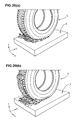
- Figs. 20 (a) and (b) are visualized the tire model 2 and muddy road model 6 during rolling simulation.
- Fig. 20(b) follows Fig. 20(a) with time and shows that muddy volumes are visible adhering on the surface of tire model 2.
- the tire model 2 is made to roll on a stationary muddy road model 6.
- a tire model 2 with a free rotating tire axis is driven by friction force from a moving muddy road model 6 in contact with the tread of the tire model 2.
Landscapes
- Engineering & Computer Science (AREA)
- Physics & Mathematics (AREA)
- Theoretical Computer Science (AREA)
- General Physics & Mathematics (AREA)
- Geometry (AREA)
- General Engineering & Computer Science (AREA)
- Computer Hardware Design (AREA)
- Evolutionary Computation (AREA)
- Software Systems (AREA)
- Computational Mathematics (AREA)
- Mathematical Analysis (AREA)
- Mathematical Optimization (AREA)
- Pure & Applied Mathematics (AREA)
- Aviation & Aerospace Engineering (AREA)
- Automation & Control Theory (AREA)
- Mechanical Engineering (AREA)
- Tires In General (AREA)
Abstract
A method for tire rolling simulation on mud comprises the steps of modeling a tire using finite elements to build a tire model, modeling a muddy road using finite volumes to build a muddy road model which can exhibit elastoplasticity property and failure property, and executing a numerical simulation in which the tire model is made to roll on the muddy road model in a predetermined condition.
Description
- The present invention relates to a method for tire rolling simulation capable of predicting a tire performance on mud.
- conventionally, tires have been developed by a procedure of prototype manufacturing, actual testing, and improved product manufacturing based on the results of the tests. This approach, however, is inefficient because prototype manufacturing and testing demand a lot of cost and time. To solve this drawback, computer simulation using a numerical analysis method, such as the finite element method, have been suggested. This approach enables the prediction of tire performance without manufacturing prototype tires.
- Conventional simulation, however, is only performed on dry asphalt, wet asphalt, or sandy roads in which volume change remains, such as snow or desiccated soil. Therefore, the conventional approaches fail to accurately predict tire performance running on mud, which clings, to the tread surface of a tire.
- It is a main object of the present invention to provide a method for tire rolling simulation, which can simulate the tire performance on mud with accuracy.
- According to the present invention, a method for tire rolling simulation on mud comprises the steps of
modeling a tire using finite elements to build a tire model,
modeling a muddy road covered with mud using finite volumes to build a muddy road model which can exhibit elastoplasticity property, and failure property in which the finite volume fails under a certain tensile stress, but does not fail under any compression stress, and
executing a numerical simulation in which the tire model is made to roll on the muddy road model in a predetermined condition. -
-
Fig. 1 is an illustration of a computer device for executing the simulation method; -
Fig. 2 is a flowchart showing an example of the simulation method; -
Fig. 3 is a perspective view of a tire model; -
Fig. 4 is a side view of the tire model in another embodiment; -
Fig. 5 is a perspective view explaining the modeling of cord reinforcements; -
Fig. 6 is a side view, which visualizes an example of a muddy road model; -
Figs. 7(a) and 7(b) are side views showing an interaction between the tire model and the muddy road model; -
Fig. 8 is a cross-sectional view of a compression test machine for mud; -
Fig. 9 is a graph showing a typical relationship between the deviatoric stress and plastic compressive strain of mud; -
Fig. 10 is a front cross-sectional view of a hollow cylinder tensile test machine for mud; -
Figs. 11 (a) and 11(b) are cross-sectional views perpendicular to axis center line, and showing failure of mud in the cylinder of the hollow cylinder tensile test machine; -
Fig. 12 a graph showing a result of the cylinder of the hollow cylinder tensile tests; -
Figs. 13 (a) and 13(b) are schematic illustrations showing each equilibrium of force between the tire model and the muddy road model. -
Fig. 14 is a cross sectional view of the tire model; -
Fig. 15 is a perspective view of an element in the tire model; -
Fig. 16 is a flowchart showing an example of the deformation calculation of the tire model; -
Fig. 17 is a flowchart showing an example of the deformation calculation of the muddy road model; -
Fig. 18 is a graph showing the relationship between pressure and deviatoric stress; -
Fig. 19 is a graph showing the relationship between plastic strain and deviatoric stress; and -
Figs. 20(a) and 20(b) are visualized perspective views of tires on rolling simulation. - An embodiment of the present invention will be described as follows based on the drawings.
- The simulation method of this embodiment is to roll a
tire model 2 on a road covered with thick mud layer. Here, mud comprises a mixture of mud particles of at least one kind of: clay having a particle size of less than 0.005 mm; silt having a particle size of from 0.005 to 0.075 mm; fine mud having a particle size of from 0.075 to 0.250 mm; medium mud having a particle size of from 0.250 to 0.850 mm; fine gravel having a particle size of from 0.850 to 2.00 mm; granule having a particle size of from 2.00 to 4.75 mm; or medium gravel having a particle size of from 4.75 to 19.00 mm. In order to set a muddy road condition, the particle size is preferably not more than 9.50 mm, and percentage of water content is preferably set in the range of from 10 to 50%, more preferably in the range of from 10 to 40%. -
Fig. 1 shows acomputer device 1 used for the simulation method of the present invention. Thecomputer device 1 comprises amain body 1a, akeyboard 1b, amouse 1c, and adisplay device 1d. Themain body 1a includes disk drives 1a1 and 1a2, a CPU, a ROM, a memory, and a bulk storage (which are not illustrated). The bulk storage stores programs, which execute the simulation method described below. -
Fig. 2 shows an example of the procedure of the invention simulation method. In the step s1, atire model 2 is set by modeling a tire using finite elements capable of numerical analysis. The numerical analysis includes, for example, the finite element method, the finite volume method, the finite difference method and the boundary element method. In this example, the finite element method and the finite volume method are employed. -
Fig. 3 is an example of thetire model 2 which is visualized in three-dimensional. In thetire model 2, the tire to be analyzed is divided into a finite number of small elements (LaGrange elements) 2a, 2b, 2c which are numerical data capable of calculation by thecomputer device 1. Further, thetire model 2 includes the coordinate values of the nodal points of eachelement elements - Most of the rubber part of the tire is modeled using mainly three-dimensional solid elements. The
tire model 2 shown inFig. 3 is provided with tread grooves on the tread including longitudinal and transverse grooves, but these may be omitted. The circumferential length of one element arranged on the tread of thetire model 2 does not preferably exceed 25% of a circumferential length of the tread ground contact portion. This is useful for correct expression of the tread ground contact pressure or the distribution of the shearing force. The length of one element in the axial direction of the tire is preferably 20 mm or less. - As shown in
Fig. 4 , thetire model 2 could be, but not limited to, a combination of the detailed pattern part "A" that has modeled grooves on the tread and the simple pattern part B that has no grooves on the tread. The detailed pattern part "A" is longer than the tread ground contact portion in the tire circumferential direction, but is shorter than the simple pattern part B. This helps to accelerate the calculation time by reducing the number of elements in thetire model 2 as a whole. -
Fig. 5 shows an example of modeling of a cord reinforcement member c such as a belt ply, a carcass ply or the like. The cord reinforcement members c are modeled intomembrane elements solid elements shell element 5. Themembrane elements - In the Step S2 shown in
Fig. 2 , a muddy road model is set by modeling muddy road in finite volumes capable of the numerical analysis above. - The muddy road model is modeled in this embodiment using Euler finite volumes.
Fig. 6 shows an example of themuddy road model 6. Themuddy road model 6 comprises: a three-dimensional regularfinite volume mesh 6a fixed on thestiff element 7; and thenumerical mud material 6c corresponding to the mud packed in thespaces 6b divided by themesh 6a. - The
mud material 6c can move in thespace 6b of themesh 6a having a bottom and sidewalls. The thickness H of themud material 6c corresponds to the thickness of the mud layer to be evaluated. In this embodiment, the thickness is taken large enough to represent deep mud. Here, the term "one volume of the muddy road model" means onehexagonal space 6b and thenumerical mud material 6c therein. - Further, the
muddy road model 6 has a width and a length as necessary for the rotation of thetire model 2. -
Figs. 7(a) and 7 ((b) show a state in which themuddy road model 6 gets into contact with thetire model 2. In the deformation calculation of thetire model 2 andmuddy road model 6 described later, the crossing portion J between thetire model 2 and thenumerical mud material 6c is calculated based on mutual position information. Then, thetire model 2 and themud material 6c are coupled at the boundary JL of the crossing portion J so as to interact with each other. Namely, themud material 6c provides reaction force to thetire model 2 through the boundary JL. On the other hand, thetire model 2 provides themud material 6c with a moving boundary surface (coupling surface). Therefore,mud material 6c in the cross portion J is moved out of the model so that themud material 6c is compressed along the tread of the tire model. - Further, elastoplasticity property, failure property, and adhesion are defined in the
mud material 6c. - The elastoplasticity is a state of a substance subjected to a stress greater than its elastic limit but not so great as to cause it to rupture, in which it exhibits both elastic and plastic properties. Namely, the
numerical mud material 6c can change its physical property according to its state of the stress. The inventors have found that the behavior of mud with, but not limited to, a particle size can be represented by elastoplasticity. That is, the mud hasviscosity, so that the deformation property thereof is dependent on the strain rate. - The elastoplasticity is preferably to be set according to mud properties that are to be evaluated for the target mud. In this embodiment, in order to satisfy this requirement, the elastoplasticity of the mud is determined based on results of the triaxial compression tests in which the mud is compressed with an axial force under an external pressure that is kept constant.
- Meanwhile, the failure property is denoted as the following characteristics: the
mud material 6c does not fail by compression stress (average compression stress) even if plastic strain occurs therein; and themud material 6c fails by tensile stress (average tensile stress) when equivalent plastic strain reaches a particular value. The equivalent plastic strain is kept constant regardless of the external pressure. - The failure property is also preferably to be set according to mud properties that are to be evaluated for the target mud. In this embodiment, in order to satisfy this requirement, the failure property of the mud is determined based on results of the hollow cylinder tensile tests.
- Accordingly, by defining the elastoplasticity and failure property into the
muddy road model 6, it is possible to obtain the tire performance on mud with high accuracy by the simulation. -
Fig. 8 schematically shows an example of acompression test machine 10 for mud. Thecompression test machine 10 comprises: apressure chamber 11 filled with a liquid such as water; acylindrical container 12 packed with mud S and placed inside thechamber 11; and anactuator 14 which can apply an axial compressive force on thecontainer 12 and the mud inside. - The
pressure chamber 11 comprises: a cylindricalmain body 11a having a space therein; anupper cover 11b to close a top of themain body 11a with aguide 11d for the piston rod of theactuator 14; and abottom cover 11c to close the bottom of themain body 11a. The internal pressure of thechamber 11 is kept constant by controlling amount of the liquid using a control device (not shown). Thebottom cover 11c is provided with a passage 11e1 connecting the bottom of thecontainer 12 to the control device and a second passage 11e2 connected to a pressure gage (not shown). - The
cylindrical container 12 has a thin and soft sidewall made of rubber or the like such that it does not have substantial stiffness. In this embodiment, thecontainer 12 has a diameter of about 5cm. Further, test mud s is tightly packed in thecontainer 12. Therefore, the mud s receives pressure from the liquid in thechamber 11 through the soft sidewall of thecontainer 12. Further, the bottom of thecontainer 12 is fixed on thelower cover 11c, and its top is pushed by the piston rod of theactuator 14. Also, the sidewall of thecontainer 12 receives liquid pressure in thechamber 11. The liquid pressure in thechamber 11 is defined as external pressure for the mud S. - since the physical property of mud varies according to the stress state thereof, it is desirable that the compression test is performed under at least two, or preferably three different levels of external pressure acting on mud. Further, the levels of external pressure are preferably determined in consideration of the contact pressure of the tire. In this embodiment, the mud compression tests have been performed under three levels of external pressure of 98 kPa, 196 kPa, and 294 kPa, respectively.
- In this triaxial compression test, the following steps are performed: setting the external pressure being applied to the
container 12; compressing thecontainer 12; and measuring various parameters such as the force, the displacement and/or the volume change of the mud. - In such a compression test, the mud s filled in the
container 12 is in a triaxial stress state receiving external pressure in x, Y, and z directions and compressive axial force in z direction from theactuator 14. under a constant external pressure, when increasing the axial force, particles of the mud begin to slip, and then thecontainer 12 bulges in its radial direction. As shown inFig. 9 , the relationship between the axial stress and the axial plastic compression strain of the mud is obtained from the result of these compression tests. - The
actuator 14 is pressed down by the velocities ε'1 and ε'2 (> ε'1) under each of the three leveled external pressures to reflect strain velocity in the simulation. - More specifically, the vertical axis in
Fig. 9 shows the deviatoric stress (σa-σr) of the mud, and the horizontal axis shows the axial plastic compression strain εa of the mud. These are calculated as follows.
- L0: Original axial length of the mud filled in the container
- ΔL: Change of axial Length of the mud
- σa: Maximum principal stress (= Fext/A)
Fext : axial compressive force
A : Current nominal cross-section area of the mud filled in the container - σr: minimum principal stress (=external pressure acting on mud)
- Sliding is started between the particles having smaller contact force and gradually increases as the deviatoric stress increases, until complete sliding occurs at the peak of the axial stress-strain curve. This sliding also causes the increase of the stress to slow down. This means that mud exhibits elastoplasticity. As sliding continues after the peak of the axial stress, the axial stress decreases slowly until it is saturated.
-
Fig. 9 shows that the relationship between the axial plastic compression strain εa and the deviatoric stress (σa-σr) of the mud s varies according to the external pressure. That is, when the compression velocity is higher, the deviatonic stress is also higher. The strain rate dependency appears prominently. - Further, in each of the six curves shown in
Fig. 9 , in this embodiment, the stress-strain relationship, namely the elastoplasticity, under three different levels of external pressures and two different levels of strain velocities as obtained in the compression tests, is defined as the elastic-plastic relationship of themuddy road model 6. In other words, in the simulation step, each finite volume of themuddy road model 6 behaves according to the relationship shown inFig. 9 . Further, thecomputer device 1 depicts these curves shown inFig. 9 as functions and/or approximate curves and stores them. In the elastoplasticity inFig.9 , the stress-strain relationship excepting under each of the above mentioned predetermined levels of external pressures and strain velocities can be obtained by interpolation. -
Fig. 10 shows an embodiment of atensile test machine 20 for hollow cylinder tensile tests to study the failure property of mud. Thetensile test machine 20, as well as the triaxialcompression tests machine 10, comprises: - a
pressure chamber 21 filled with a liquid w such as water; acylindrical container 22 having a hollow (i) therein and packed with mud s and placed inside thechamber 21; and - an
actuator 23 which can apply an axial compressive force on thecontainer 22 and the mud s. - The
container 22 has a thin and soft sidewall made of rubber or the like such that it does not have substantial stiffness. Thepressure chamber 21 comprises: anupper cover 21a and abottom cover 21b. Theupper cover 21a having aflow channel 25 to inflate high-pressure air from a pressure pump P so as to the outer surfaces of thecontainer 22 can be applied a pressure Po through the liquid W. Thebottom cover 21b having aflow channel 26 to inflate high-pressure air from a pressure pump P into the hollow (i) so as to apply arbitrary pressure Pi on the surface of the mud S from the side of the hollow (i). - The actions of the
tensile test machine 20 are described below. As shown inFig. 11(a) , certain pressures Pi and Po were applied into thepressure chamber 21 and the hollow (i) ofcontainer 22, respectively. And, theactuator 23 presses thecontainer 22 so that the compression pressure applied to thecontainer 22 is as much as the external pressure Po. While keeping the pressure Po of thepressure chamber 22 constant, the pressure Pi in the hollow (i) of thecontainer 22 is increased until cracks Sc occurring in the mud s of thecontainer 22 as shown inFig. 11(b) . The pressure P of theactuator 23 is supplemented with the pressure increasing in the hollow (i). Amanometer 27 and aflow meter 28 measure the internal pressure Pi and volume increases of thecontainer 22, respectively. In the present embodiment; the hollow cylinder tensile tests have been performed under two levels of external pressure Po of 19.6 kPa and 98.0 kPa. - Mud is unfit for a conventional tensile test. However, the present embodiment allows to test its failure property. In the present embodiment, the mud is contained in the ring-shaped hollow
cylindrical container 22; the hollow (i) thereof is applied pressure; and the mud is applied the tensile stress in the circumferential direction until failing. -
Fig. 12 shows the results of the above-described hollow cylinder tensile tests. The volume of the hollow (i) gradually increases in accordance with the increase of the inner pressure Pi initially. Then, the inner pressure Pi hardly increases, however, the volume of the hollow (i) suddenly increases, and finally yields and then fails. Meanwhile, the failure strain does not depend on the external pressure but is constant. In the present embodiment, the failure strain is stored in thecomputer device 1. - unlike snow and sand, mud has strong adhesion. When the tire rolls on such a muddy road surface, the mud adheres on the tread surface of the tire. The mud adhered thereon is pulled by the tire and comes off the road surface. Such a condition is represented in the computer simulation of the present embodiment. In other words, the volume of the
mud model 6 gets out when the equivalent plastic strain thereof is over the certain value predetermined based on the failure property under tensile stress condition, so that it is useful in simulating accurately the representation of rolling resistance caused by mud. Adhesion frictional force between the tire surface and the mud occurs also in the tensile stress condition. The adhesion force and adhesion frictional force are predetermined between thetire model 2 andmuddy road model 6, and these forces are considered in the deformation calculation for simulation. -
Fig. 13(a) shows a schematic illustration wherein thetire model 2 and themuddy road model 6 are in compression. In this instance, vertical reactive force N and frictional force µN that is caused by locomotion (µ: coefficient of dynamic friction) arise. These forces affect on thetire model 2. - As shown in
Fig. 13(b) , when thetire model 2 andmuddy road model 6 are in the tensile stress condition, thetire model 2 is subjected to adhesive force and frictional force that is caused by locomotion (hereinafter called "adhesion frictional force") βF. - β: A variable depending on slip velocity (<=1)
- F: A predetermined maximum adhesion frictional force
- The adhesive force is normal force, arises ongoingly, and continues to increase to the break point of the
mud material 6c of themuddy road model 6. Moreover, the adhesive force is set to be particularly larger than the breaking strength of themuddy road model 6. - Meanwhile, the adhesion frictional force is a force perpendicular to the above-mentioned adhesive force, and continues to generate until it reaches maximum frictional force. In this way, the simulation with this generation of frictional force under the tensile stress condition, in view of the adhesive force, can represent more accurately the condition of tire rolling in muddy road.
- Next, in step s3 in this present embodiment, boundary conditions for the simulation are set. The boundary conditions include wheel rims, internal pressure of the
tire model 2, friction coefficient between thetire model 2 and themuddy road model 6, the tire load, the slip angle, the camber angle, rotating speed (In this embodiment, rotational and translational speeds are set to thetire model 2.), initial time increment for deformation calculation of each model and initial position of eachmodel -
Fig. 14 shows the virtual rim assembly of thetire model 2. A pair ofbead regions 2r of thetire model 2 are equal to the rim width. The radial distance (r) from the rotation axis CL of thetire model 2 to thebead regions 2r is set to be equal to the rim diameter. Further, the internal pressure is expressed by applying an uniformly distributed load (w) having the same value as the internal pressure of the tire on the internal surface of thetire model 2. - Next, in the steps s4 to s8, deformation calculations of the
tire model 2 and the muddy road model are performed. Namely, the state where thetire model 2 rolls on themuddy road model 6 is calculated for every small time increment by using thecomputer device 1. - The explicit time integration method is employed in the simulation in this present example. According to the explicit method, the moment that the load acts on each model is taken as time zero, and the time is divided into small increments so as to find the displacement of the model at each point in time. The explicit method does not involve convergence calculations. However, it is necessary that the time increment satisfies the "Courant criterion", in order to stabilize the calculations. To be more specific, the initial time increment Δt in the deformation calculation for the
tire model 2 and themuddy road model 6 is set at the values that meet the following formula (1).
- Here, "Lmin" is the characteristic length of the smallest element in each model, and "C" is the propagation speed of a stress wave propagating in the material calculated as follows:

where E is Young's modulus, and ρ is the density. In the deformation calculations with a time increment that satisfies the Courant criterion, as shown inFig. 15 , it becomes possible to calculate the deformation condition of the element e1 when an external force F acts thereon before the external force F is transferred to the element e2 adjacent to the element e1. This helps to obtain stable solutions. - In this embodiment, the propagating time of the stress wave of each element is calculated based on the formula (1), and after that, the time increment is set up by multiplying the minimum of the propagating time by a safety factor. The safety factor is, for example, more preferably set equal to 0.66. Further, the initial time increment is preferably set of from 0.1 to 5 µsec, more preferably 0.3 to 3 µsec, and most preferably 0.5 to 2 µsec for both the
tire model 2 and themuddy road model 6. - As shown in the Steps S4 to S8 in
Fig.2 , the deformation calculation of thetire model 2 and the deformation calculation of themuddy road model 6 are performed separately. However, the position, the shape and the speed data of thetire model 2 obtained from the deformation calculation of thetire model 2 are given to themuddy road model 6 as a boundary condition for the deformation calculation of the muddy road model 6 (Step S8). On the other hand, the pressure and frictional force obtained from the deformation calculation of themuddy road model 6 are given to thetire model 2 as the boundary condition (load) for the deformation calculation of the tire model 2 (Step S7). -
Fig. 16 shows an example of the deformation calculation of thetire model 2. In Step S41 shown inFig. 16 , the deformation calculation after the time increment Δt is performed first. The deformation calculation in the present example is performed by thecomputer device 1 to solve equations of motion. Calculated values indicate the state that the tire rolls on themuddy road model 6 for the time increment Δt. - Next, the stress wave propagation time of each element of the
deformed tire model 2 is calculated based on its size, density and stiffness (Step S42). Then, based on the minimum value of this stress wave propagation time, the time increment for the next deformation calculation is set so as to satisfy the Courant criterion above (Step S43). Since the stress wave propagation time is a function of the size and density of the element, it changes every time the element deforms. In the present embodiment, the optimum time increment is set in accordance with the deformation of the element, which helps the deformation calculation of thetire model 2 to be performed more accurately. - Next, it is checked whether the predetermined duration of simulation time has been elapsed or not (Step S44). When "No" is selected in the Step S44, the process goes back to the Step S41 to perform one more calculation by adding the newly set time increment. When "Yes" is selected in the Step S44, the deformation calculation of the
tire model 2 is terminated and the process goes to the Step S6. -
Fig. 17 shows an example of the deformation calculation of themuddy road model 6. The deformation calculation of the material in each finite volume of themuddy road model 6 is performed after the time increment (Step S51). In this Step 51, the density ρ of each finite volume of themuddy road model 6 is calculated because the density of themud material 6c of themuddy model 6 changes in accordance with positions of thetire model 2. - The volume strain εv is calculated by the following formula (2) using the current density pof each finite volume of the
muddy road model 6.
- Here, ρ0 is the initial density of the finite volume under zero pressure, and the compressive volume strain is expressed as negative.
- Next, the pressure P after the time increment passed is calculated by the following formula (3).

- The pressure P is the average value of the three normal stress components that act on each finite volume. Further, "a1" and "a2" are material parameters, µ is the volume-compression rate (compression is positive) defined by the following formula (4).

- Next, the stress calculation of the
muddy road model 6 after the time increment is performed (Step S52). In this stress calculation, the second invariant J2 of the stress tensor of each finite volume of themuddy road model 6 are calculated using deviatoric stresses of each volume. Each of the normal deviatoric stresses σx', σy', and σz' is calculated by subtracting the pressure P evaluated above from each of the normal stresses, σx, σy, and σz.


- The second invariant J2 of the stress tensor is calculated by the following equation (8) using the above deviatoric stress and shear stress components.

- In this equation, τxy, τyz, and τzx are the shear stress components. In this step, strain increments of each finite volume is considered as elastic.
- Next, the stress-strain curve of each finite volume of the
muddy road model 6 after the time increment is calculated. Since the pressure P of each finite volume has already been calculated in Step S51, the stress-strain curve corresponding to the pressure P and the strain rate is obtained based on the predetermined elastoplastic stress-strain curve shown inFig. 9 (Step S53). - In Step S54, it is checked whether the present stress state of each finite volume is over the stress-strain curve or not. When it has been determined that the stress of the volume is over the stress-strain curve, an iteration process for decreasing the stress is performed in Step S55.
-
Fig. 18 shows the relationship between a parameter (3J2)0.5 using the second invariant J2 and the pressure P.Fig. 19 shows the relationship between the parameter (3J2)0.5 and the plastic strain εp. - Namely, in the deformation calculation of the muddy road model in the step S52, all the increase in each volume of the
muddy road model 6 is assumed to be caused by elastic deformation. The step S54 is therefore needed for verifying correctness of the above-mentioned assumption. When the value of stress state of the volume is over the stress-strain curve, it is necessary to reduce the value to a correct value on the stress-strain curve while recalculating the elastic and plastic deformation and the pressure so as to keep the simulation accuracy high. - To describe an example of Steps S54 and S55, a finite volume is now assumed in a state of z1 and the stress-strain curve is assumed as the curve f2' as shown in
Fig. 19 . The state of z1 of the finite volume is over the curve f2'. This means that the deformation of the material is in a plastic region, and an iteration step is performed. - The iteration process may be performed in various ways; in this embodiment the iteration process to decrease the stress of the finite volume is performed until the state z1 becomes on the stress-strain curve. Specifically, the process decreases the stress of the finite volume to state Z' to the stress-strain curve f2' without changing the plastic strain εp1 of the state z2'.
- Next, a new plastic strain εp2" is obtained by considering the strain caused by reducing the stress from the state z1 to z2' as a plastic component. In the iteration process, the strain corresponding to the difference between the stress state z1 and the stress-plastic strain curve f2' is regarded as a component of the plastic strain causing plastic deformation to the finite volume.
- Next, a new pressure P of the finite volume and the strain velocity are calculated using the stress state of z2'. Then, a new stress-strain curve f2" is calculated based on the latest pressure P and the relationship of
Fig. 9 . Then, a new stress state z2" with a plastic strain εp2" which lies on the stress-strain curve f2" is calculated. Further, the plastic strain and the pressure of the finite volume are recalculated, and these process continues until the stress state of the finite volume converges on the stress-strain curve. Accordingly, the stress state z1 of the finite volume is finally decreased to the stress state z2 on the stress-strain curve f2. - In
Step 56, when the average stress of a finite volume of themuddy road model 6 is tensile force, the equivalent plastic strain of the volume is compared to the predetermined failure strain of failure condition. If the value of equivalent plastic strain is larger than that of the failure strain, the stress of the volume is set to be zero (Step 57). - The adhesive force is sufficiently-larger than the failure breaking strength. The volume after
Step 57 therefore pulls out of themuddy road model 6 and attaches to thetire model 2 owing to the adhesive force. Meanwhile, when the volume of mud attached to thetire model 2 connects again to ground and that the average strain increment get back tocompression, the mud volume can regenerate stress. - In this way, considered are the travel resistance caused by mud addressing and the detachment from a road surface caused by mud fracturing in the simulation.
- In this embodiment, the stress wave propagation time of each finite volume of the deformed
muddy road model 6 is recalculated, and a value equal to the minimum value of the stress wave propagation time multiplied by the safety factor is set as the next time increment (Step S58). - Next, it is checked whether the predetermined simulation duration has elapsed or not (Step S59). When it has not, the process goes back to Step S51 and recalculation is performed again with the newly set time increment. When it has elapsed, the deformation calculation of the
muddy road model 6 is terminated to return to Step s6 ofFig.2 . - In Steps S7 and S8 in
Fig.2 , necessary data obtained from the results of the individual calculations of thetire model 2 andmuddy road model 6 are exchanged between these models so as to couple them. The pressure data of themuddy road model 6 is given to thetire model 2 as a load for next deformation calculation thereof. On the other hand, the shape and speed of thetire model 2 are given to themuddy road model 6 as a boundary condition for the next deformation calculation thereof. - Accordingly, it becomes possible for the
muddy road model 6 to calculate changes in the reaction force on thetire model 2 due to changes in the position or shape of thetire model 2. For thetire model 2, it becomes possible to calculate a new deformation due to the reaction force received from themuddy road model 6. Repeating these calculations can analyze the changing contact situation between thetire model 2 and themuddy road model 6, while considering their interaction. - In Step S6, it is checked whether the predetermined duration that indicates the completion of calculation has elapsed or not. When "Yes" is selected in Step S6, the calculation results are outputted (Step S9), and the simulation procedure is terminated. The duration of the calculations in Step S6 can be determined according to the simulation to be executed so as to obtain stable calculation results.
- The output of the calculation results may contain various information. For example, pressure and plastic strain distribution of the
muddy road model 6 and longitudinal and/or side force applied on thetire model 2 may be obtained. Any physical parameters involved in thetire model 2 and themuddy road model 6 calculations may be obtained as output information. -
Figs. 20 (a) and (b) are visualized thetire model 2 andmuddy road model 6 during rolling simulation.Fig. 20(b) followsFig. 20(a) with time and shows that muddy volumes are visible adhering on the surface oftire model 2. - Based on the outputted information of the simulation, designers and analysts can device modifications of internal structure of tire, profile of tread, tread grooves, tread patterns or sipes, internal pressure of tire, and used rubber materials. It is also possible to prototype the tire version that have shown preferable simulation results. This greatly accelerates the process of development of tires for mud, thereby reducing the development time and cost.
- In this embodiment described above, the
tire model 2 is made to roll on a stationarymuddy road model 6. However, it is possible that atire model 2 with a free rotating tire axis is driven by friction force from a movingmuddy road model 6 in contact with the tread of thetire model 2.
Claims (6)
- A method for tire rolling simulation on mud comprising the steps of:modeling a tire using finite elements to build a tire model;modeling a muddy road covered with mud using finite volumes to build a muddy road model which can exhibit elastoplasticity property, and failure property in which the finite volume fails under a certain tensile stress, but does not fail under any compression stress; andexecuting a numerical simulation in which the tire model is made to roll on the muddy road model in a predetermined condition.
- The method for tire rolling simulation on mud according to claim 1, wherein
travel resistance is reproduced by predetermining adhesion and traction between said tire model and muddy road model in the step of executing a numerical simulation. - The method for tire rolling simulation on mud according to claim 1, wherein
the elastoplasticity is defined using a predetermined relationship between the stress and the strain of the mud, and
the relationship is obtained from triaxial compression tests in which the mud is compressed with an axial force under at least two different levels of external constant pressure. - The method for tire rolling simulation on mud according to claim 3, wherein
the relationship between the stress and strain of the mud has a first region and a second region,
the first region exhibits a smooth increase of strain with increase of the stress, and
the second region exhibits a smooth increase of stress from the yield point with increase of the strain. - The method for tire rolling simulation on mud according to claim 1, wherein
said failure property is defined using the steps of:executing hollow cylinder tensile tests, the test comprising the steps of
forming a hollow cylinder by using mud, and
destroying the hollow cylinder by increasing internal pressure under at least two different levels of external constant pressure; andcalculating failure strain based on the values obtained by hollow cylinder tensile tests. - The method for tire rolling simulation on mud according to claim 1, wherein said simulation comprising the steps of:calculating stress of said each finite volume of the muddy road model;calculating a curve of relation between the stress and plastic strain;determining whether said each stress of the volume is over the value on the stress-strain curve or not; andwhen the stress value of the volume is over the stress-strain curve, the stress value is modified on a value of the stress-strain curb.
Applications Claiming Priority (1)
| Application Number | Priority Date | Filing Date | Title |
|---|---|---|---|
| JP2008155683A JP4659070B2 (en) | 2008-06-13 | 2008-06-13 | Tire running simulation method |
Publications (1)
| Publication Number | Publication Date |
|---|---|
| EP2157521A1 true EP2157521A1 (en) | 2010-02-24 |
Family
ID=41396321
Family Applications (1)
| Application Number | Title | Priority Date | Filing Date |
|---|---|---|---|
| EP09006542A Withdrawn EP2157521A1 (en) | 2008-06-13 | 2009-05-14 | Method for tire rolling simulation on mud |
Country Status (5)
| Country | Link |
|---|---|
| US (1) | US7908915B2 (en) |
| EP (1) | EP2157521A1 (en) |
| JP (1) | JP4659070B2 (en) |
| KR (1) | KR20090129940A (en) |
| CN (1) | CN101603882B (en) |
Families Citing this family (15)
| Publication number | Priority date | Publication date | Assignee | Title |
|---|---|---|---|---|
| JP5588378B2 (en) * | 2011-02-28 | 2014-09-10 | 住友ゴム工業株式会社 | How to evaluate tire mud performance |
| JP5811625B2 (en) * | 2011-06-22 | 2015-11-11 | 横浜ゴム株式会社 | Simulation method and simulation apparatus |
| JP5848550B2 (en) * | 2011-08-24 | 2016-01-27 | 住友ゴム工業株式会社 | Tire mud performance evaluation method |
| US8960003B2 (en) * | 2011-09-16 | 2015-02-24 | Taiwan Semiconductor Manufacturing Company, Ltd. | Motion sensor device and methods for forming the same |
| JP6039167B2 (en) * | 2011-09-20 | 2016-12-07 | 住友ゴム工業株式会社 | Tire simulation method |
| KR101675362B1 (en) | 2012-04-11 | 2016-11-11 | 브리지스톤 어메리카스 타이어 오퍼레이션스, 엘엘씨 | System and method for steady state simulation of rolling tire |
| JP5613195B2 (en) * | 2012-04-11 | 2014-10-22 | 住友ゴム工業株式会社 | Tire simulation method |
| JP6093157B2 (en) * | 2012-11-27 | 2017-03-08 | 住友ゴム工業株式会社 | Syringe design method |
| CN103076191B (en) * | 2013-01-10 | 2014-12-24 | 中国矿业大学 | Shock excitation abrasion tester for tyre in complex environment |
| CN104344967B (en) * | 2014-02-28 | 2017-01-18 | 风神轮胎股份有限公司 | Tread pattern groove pumping noise source recognition method |
| US10179487B1 (en) * | 2016-01-15 | 2019-01-15 | Hunter Engineering Company | Method for generating images of predicted tire tread wear |
| JP6668774B2 (en) * | 2016-01-20 | 2020-03-18 | 横浜ゴム株式会社 | Simulation method and evaluation method of pneumatic tire |
| US10549587B2 (en) | 2017-10-19 | 2020-02-04 | Infineon Technologies Ag | Method, component, tire-mounted TPMS module, TPMS system, and machine readable storage or computer program for determining time information of at least one contact patch event of a rolling tire, method for locating a tire |
| US20190118592A1 (en) * | 2017-10-19 | 2019-04-25 | Infineon Technologies Ag | Method, Tire-Mounted TPMS Component, and Machine Readable Storage or Computer Program for Determining a Duration of at Least one Contact Patch Event of a Rolling Tire |
| CN112033624B (en) * | 2020-09-23 | 2022-09-27 | 赛轮集团股份有限公司 | Device for measuring ground pressure distribution of tire in coating state |
Citations (2)
| Publication number | Priority date | Publication date | Assignee | Title |
|---|---|---|---|---|
| EP1297975A1 (en) * | 2000-06-14 | 2003-04-02 | Sumitomo Rubber Industries, Ltd. | Vehicle/tire performances simulating method |
| EP1777634A1 (en) | 2005-10-24 | 2007-04-25 | Sumitomo Rubber Industries, Ltd. | Method for tire rolling simulation on sand |
Family Cites Families (7)
| Publication number | Priority date | Publication date | Assignee | Title |
|---|---|---|---|---|
| JP2887977B2 (en) * | 1991-10-01 | 1999-05-10 | 三菱マテリアル株式会社 | Fracture toughness test method and fracture toughness test apparatus |
| JP3332370B1 (en) * | 2001-09-18 | 2002-10-07 | 住友ゴム工業株式会社 | Tire running simulation method |
| JP4394866B2 (en) * | 2002-07-02 | 2010-01-06 | 住友ゴム工業株式会社 | Tire running simulation method |
| JP2004042831A (en) * | 2002-07-12 | 2004-02-12 | Sumitomo Rubber Ind Ltd | Simulation method for running tires on snow |
| JP2005351770A (en) * | 2004-06-10 | 2005-12-22 | Sumitomo Rubber Ind Ltd | Simulation method for rubber material |
| JP4486105B2 (en) * | 2007-03-30 | 2010-06-23 | 株式会社ブリヂストン | Tire performance prediction method, ground simulation method, tire design method, recording medium, and tire performance prediction program |
| JP4746584B2 (en) * | 2007-04-27 | 2011-08-10 | 株式会社ブリヂストン | Tire performance prediction method, tire design method, recording medium, and tire performance prediction program |
-
2008
- 2008-06-13 JP JP2008155683A patent/JP4659070B2/en not_active Expired - Fee Related
-
2009
- 2009-04-24 US US12/429,698 patent/US7908915B2/en not_active Expired - Fee Related
- 2009-05-12 KR KR1020090041310A patent/KR20090129940A/en not_active Withdrawn
- 2009-05-14 EP EP09006542A patent/EP2157521A1/en not_active Withdrawn
- 2009-05-27 CN CN2009101455554A patent/CN101603882B/en not_active Expired - Fee Related
Patent Citations (2)
| Publication number | Priority date | Publication date | Assignee | Title |
|---|---|---|---|---|
| EP1297975A1 (en) * | 2000-06-14 | 2003-04-02 | Sumitomo Rubber Industries, Ltd. | Vehicle/tire performances simulating method |
| EP1777634A1 (en) | 2005-10-24 | 2007-04-25 | Sumitomo Rubber Industries, Ltd. | Method for tire rolling simulation on sand |
Non-Patent Citations (2)
| Title |
|---|
| BERKER A ET AL: "Phenomenological models of viscoplastic, thixotropic, and granular materials", RHEOLOGICA ACTA GERMANY, vol. 31, no. 2, March 1992 (1992-03-01), pages 119 - 138, XP002560260, ISSN: 0035-4511 * |
| ROONEY T ET AL: "Application of finite element analysis and computational fluid dynamics to ATV tire design", TIRE SCIENCE AND TECHNOLOGY, TIRE SOCIETY INC, US, vol. 30, no. 3, 1 January 2002 (2002-01-01), pages 198 - 212, XP009126290, ISSN: 0090-8657 * |
Also Published As
| Publication number | Publication date |
|---|---|
| US20090308149A1 (en) | 2009-12-17 |
| KR20090129940A (en) | 2009-12-17 |
| JP4659070B2 (en) | 2011-03-30 |
| CN101603882A (en) | 2009-12-16 |
| CN101603882B (en) | 2013-06-26 |
| JP2009300278A (en) | 2009-12-24 |
| US7908915B2 (en) | 2011-03-22 |
Similar Documents
| Publication | Publication Date | Title |
|---|---|---|
| US7908915B2 (en) | Method for tire rolling simulation on mud | |
| EP1293917B1 (en) | A method for tire rolling simulation | |
| El-Sayegh et al. | Improved tire-soil interaction model using FEA-SPH simulation | |
| US7343788B2 (en) | Method for tire rolling simulation on sand | |
| US20040107081A1 (en) | Method of simulating tire and snow | |
| JP4469172B2 (en) | Tire simulation method | |
| JP5430198B2 (en) | Tire wear simulation method, apparatus, and program | |
| Hernandez et al. | Numerical prediction of three-dimensional tire-pavement contact stresses | |
| EP1798648B1 (en) | Method for pneumatic tire simulation | |
| JP4594030B2 (en) | Tire performance prediction method, tire simulation method, tire performance prediction program, and recording medium | |
| JP4394866B2 (en) | Tire running simulation method | |
| JP6634840B2 (en) | Tire simulation method | |
| JP2004042831A (en) | Simulation method for running tires on snow | |
| JP6039167B2 (en) | Tire simulation method | |
| Lardner | Prediction of the off-road rigid-ring model parameters for truck tire and soft soil interactions | |
| JP2004042832A (en) | Simulation method of tire on snow | |
| JP4486105B2 (en) | Tire performance prediction method, ground simulation method, tire design method, recording medium, and tire performance prediction program | |
| JP3305706B1 (en) | Tire running simulation method | |
| Ly et al. | Investigation of Truck Tire Rubber Material Definitions Using Finite Element Analysis | |
| JP3332370B1 (en) | Tire running simulation method | |
| JP3305705B1 (en) | Tire running simulation method | |
| Mansura et al. | A Novel Multiscale Numerical Model for Prediction of Texture-Related Impacts on Fuel Consumption | |
| Khosravi | Modeling and analysis of Regional Haul Steer (RHS) truck tire model | |
| Khosravi et al. | DEVELOPMENT AND VALIDATION OF A REGIONAL HAUL STEER (RHS) TRUCK TIRE MODEL USING ADVANCED COMPUTATIONAL TECHNIQUES | |
| JP2006309437A (en) | Device and method for simulating tire characteristic, and method for forming tire model |
Legal Events
| Date | Code | Title | Description |
|---|---|---|---|
| PUAI | Public reference made under article 153(3) epc to a published international application that has entered the european phase |
Free format text: ORIGINAL CODE: 0009012 |
|
| AK | Designated contracting states |
Kind code of ref document: A1 Designated state(s): AT BE BG CH CY CZ DE DK EE ES FI FR GB GR HR HU IE IS IT LI LT LU LV MC MK MT NL NO PL PT RO SE SI SK TR |
|
| AX | Request for extension of the european patent |
Extension state: AL BA RS |
|
| 17P | Request for examination filed |
Effective date: 20100409 |
|
| STAA | Information on the status of an ep patent application or granted ep patent |
Free format text: STATUS: THE APPLICATION IS DEEMED TO BE WITHDRAWN |
|
| 18D | Application deemed to be withdrawn |
Effective date: 20141202 |