EP2128584A2 - Pressure sensor calibration method - Google Patents
Pressure sensor calibration method Download PDFInfo
- Publication number
- EP2128584A2 EP2128584A2 EP09160941A EP09160941A EP2128584A2 EP 2128584 A2 EP2128584 A2 EP 2128584A2 EP 09160941 A EP09160941 A EP 09160941A EP 09160941 A EP09160941 A EP 09160941A EP 2128584 A2 EP2128584 A2 EP 2128584A2
- Authority
- EP
- European Patent Office
- Prior art keywords
- polynomials
- data points
- sensor
- values
- frequency
- Prior art date
- Legal status (The legal status is an assumption and is not a legal conclusion. Google has not performed a legal analysis and makes no representation as to the accuracy of the status listed.)
- Withdrawn
Links
- 238000000034 method Methods 0.000 title claims abstract description 53
- 238000004364 calculation method Methods 0.000 description 10
- 230000006870 function Effects 0.000 description 10
- 238000011156 evaluation Methods 0.000 description 7
- 238000005259 measurement Methods 0.000 description 6
- 238000012360 testing method Methods 0.000 description 3
- 239000011159 matrix material Substances 0.000 description 2
- 241001156569 Ptychosperma lineare Species 0.000 description 1
- 230000006399 behavior Effects 0.000 description 1
- 238000010276 construction Methods 0.000 description 1
- 238000012888 cubic function Methods 0.000 description 1
- 230000003111 delayed effect Effects 0.000 description 1
- 230000001419 dependent effect Effects 0.000 description 1
- 238000010586 diagram Methods 0.000 description 1
- 230000007717 exclusion Effects 0.000 description 1
- 230000003534 oscillatory effect Effects 0.000 description 1
- 238000012545 processing Methods 0.000 description 1
- 238000003672 processing method Methods 0.000 description 1
- 238000006467 substitution reaction Methods 0.000 description 1
- 230000002277 temperature effect Effects 0.000 description 1
- 230000007704 transition Effects 0.000 description 1
Images
Classifications
-
- G—PHYSICS
- G01—MEASURING; TESTING
- G01L—MEASURING FORCE, STRESS, TORQUE, WORK, MECHANICAL POWER, MECHANICAL EFFICIENCY, OR FLUID PRESSURE
- G01L27/00—Testing or calibrating of apparatus for measuring fluid pressure
- G01L27/002—Calibrating, i.e. establishing true relation between transducer output value and value to be measured, zeroing, linearising or span error determination
-
- G—PHYSICS
- G01—MEASURING; TESTING
- G01L—MEASURING FORCE, STRESS, TORQUE, WORK, MECHANICAL POWER, MECHANICAL EFFICIENCY, OR FLUID PRESSURE
- G01L19/00—Details of, or accessories for, apparatus for measuring steady or quasi-steady pressure of a fluent medium insofar as such details or accessories are not special to particular types of pressure gauges
- G01L19/04—Means for compensating for effects of changes of temperature, i.e. other than electric compensation
-
- G—PHYSICS
- G01—MEASURING; TESTING
- G01L—MEASURING FORCE, STRESS, TORQUE, WORK, MECHANICAL POWER, MECHANICAL EFFICIENCY, OR FLUID PRESSURE
- G01L27/00—Testing or calibrating of apparatus for measuring fluid pressure
-
- G—PHYSICS
- G01—MEASURING; TESTING
- G01L—MEASURING FORCE, STRESS, TORQUE, WORK, MECHANICAL POWER, MECHANICAL EFFICIENCY, OR FLUID PRESSURE
- G01L9/00—Measuring steady of quasi-steady pressure of fluid or fluent solid material by electric or magnetic pressure-sensitive elements; Transmitting or indicating the displacement of mechanical pressure-sensitive elements, used to measure the steady or quasi-steady pressure of a fluid or fluent solid material, by electric or magnetic means
Definitions
- This subject invention relates to sensors, in one example, a pressure sensor.
- a pressure indicator includes a resonant pressure transducer whose frequency changes depending upon the applied pressure.
- the relationship between the sensor input (pressure) and the sensor output (frequency changes) is not linear.
- the resonant frequency also changes as a function of temperature.
- the pressure indicator typically includes a temperature sensor and both temperature and frequency signals are input to a microprocessor. Calibration and compensation data is stored in a memory, (i.e., an EEPROM) linked to the microprocessor.
- P f F ⁇ T where F is the frequency, P is the pressure, and T is temperature.
- P a 0 + b 0 . F + c 0 . F 2 + d 0 . F 3 + a 1 ⁇ T + b 1 . F . T + c 1 . F 2 . T + d 1 . F 3 . T + a 2 ⁇ T 2 + b 2 . F . T 2 + c 2 . F 2 . T 2 + d 2 . F 3 . T 2 + a 2 ⁇ T 3 + b 3 . F . T 3 + c 3 . F 2 . T 3 + d 3 . F 3 . T 3 . T 3
- coefficients a 0 ...d 3 are calculated from the calibration data and are used to approximate the relation of F and T to the output P.
- Linear approximation schemes such as least square fit, or an exact fit from a prescribed number of data points may be used.
- the microprocessor notes the temperature and frequency of the transducer and calculates the pressure readout based on equation (2).
- this scheme has a number of limitations.
- the fit of the polynomial is dependent on the order of the polynomial chosen. Higher order polynomials provide a better fit but significantly increase the computational burden which limits the speed and accuracy of calculations.
- Cubic splines techniques have also been used to fit data. Such methods have the advantage that curvature is controlled to avoid sharp transitions. However, such methods depend on prior knowledge of curvature constraints and end point characteristics that are often unknown or too variable creating errors in the resultant fit that do not appear in the measurement data. Furthermore, the complexity of the calculation is substantial.
- the subject invention features a new processing method for a pressure sensor.
- the pressure and temperature effects of a sensor are corrected using calibration points and highly efficient and accurate algorithms.
- the method allows rapid and accurate determinations of the output of a sensor and avoids the need for double precision floating point calculations.
- the method minimizes rounding errors, results in faster signal processing, and results in lower power consumption.
- the subject invention further features a pressure sensor which incorporates the method discussed above. Moreover, the method can be employed with other types of sensors.
- the subject invention features a method of sensing pressure.
- the sensor is then used to sense an unknown pressure P ⁇ , at a temperature T ⁇ at which the sensor has a frequency F ⁇ . From the generated polynomials, several polynomials that surround T ⁇ and F ⁇ are selected.
- generating the polynomials includes employing Newton's method.
- the generated polynomials may be stored or the data points can be stored and then the polynomials are not generated until the surrounding data points are selected.
- the subject invention also features a pressure sensor comprising a resonant pressure transducer whose frequency F changes depending on the applied pressure P and the temperature T, a temperature sensor for measuring the temperature T, and a memory including stored therein data points corresponding to the sensor's frequency F at different applied pressures and temperatures.
- the processor then outputs P ⁇ .
- the subject invention features a method of determining an unknown parameter Z based on two measured parameters X and Y.
- a sensor system is accordance with the subject invention features a sensor with a parameter Y that changes depending on parameter Z and parameter X.
- a device measures parameter X.
- a memory includes stored therein data points corresponding to values of parameter Y at different values of Z and Z.
- the subject invention uses simple interpolating polynomial functions that represents the function accurately over a narrow range in one dimension.
- the full range is achieved by providing sets of such polynomials.
- Two dimensional interpolation is then realized by creating several sets of polynomials which are then combined to form a unified representation of the data.
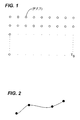
- calibration data points are collected from measurements taken to form grid of sensor characteristics in at least two variables. In one example, this would be the measurement of sensor frequency F and sensor temperature T at various applied pressures (P applied ) and test temperatures (T applied ). For example, this might be at 9 pressures and 5 temperatures yielding 45 data points as shown in Fig. 1 . There is no requirement for the grid to be either equally spaced nor contain equal number of points in each dimension. Indeed, it may be preferable to have a higher point density in areas of uncertainty.
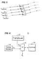
- Fig. 3 shows how 6 points create 3 cubic polynomials from 4 adjacent points.
- the polynomials may be pre-calculated and held in memory. Alternatively the defining data points alone may be held in memory and polynomial calculation delayed until it is needed.
- there are two tables of 30 polynomials related to the row/column order of the original data points instead of 9 x 5, there would be 6 x 5 i.e. 5 sets each containing 6 polynomials.
- the frequency of the transducer is F ⁇ .
- the polynomial sets that surround the point are selected. Selection of these polynomials (or their defining points) is accomplished using a simple search of the data point table held in memory. For the unknowns T ⁇ and F ⁇ , the table of polynomials is searched to find the ones which surround the unknown. In the example, four are needed for a cubic fit so that is two on either side. For the second method, only the original data is stored. So, instead of finding the four polynomials which surround T ⁇ and F ⁇ , all the points which define those polynomials are located. This would be a collection of 16 points that surround T ⁇ and F ⁇ . A cubic function suits the variability of P with T, so for any given point the four nearest sets that surround that point are selected.
- Each of these sets of polynomials can now be evaluated to give P and T values for the given value of F ⁇ using a substitution in the pre-calculated Newtonian polynomials.
- a combined interpolation and evaluation of the original data points using Lagrange's method can be employed. In this case, 16 original data points would be chosen, to create four polynomials.
- the four surrounding sets provide four values of P and four values of T for the given value F ⁇ as shown in Fig. 5 .
- Lagrange and Newton's method can be used to substantially reduce the computational power required.
- Newton's method allows a pre-calculation of all the polynomials in an accurate and efficient manner leaving only the evaluation of m+1 of these polynomials and final interpolation using Lagrange's method.
- Fig. 6 shows pressure sensor 10 having an output P and transducer 12 which generates a different frequency F when subject to different pressures.
- Temperature sensor 14 measures the temperature T.
- Processor 16 is responsive to both F and T and is configured (e.g.) programmed to operate according to the method discussed above.
- EEPROM 18 (or some other memory) stores the values of F and P at different temperatures T as discussed above in reference to Fig. 1 .
- Processor 16 outputs (to a display, for example) P ⁇ when transducer 12 is subject to P ⁇ at temperature T ⁇ and exhibits a frequency F ⁇ .
- the above method has yielded accuracy of better than 1ppm using single precision floating point calculations.
- the subject invention is not limited to pressure transducers and the method described above can be used with other types of sensors.
- This data is of the form (X,Y,Z). For example, consider a test of a pressure sensor across a range of different applied pressures and temperatures. Z is the measured pressure, X is the temperature sensor measurement and Y is the output of the sensor.
- step one the data points (X,Y,Z) are arranged to represent a grid of Z values for two input variables X and Y where X and Y are in monotonic order. See Fig. 1 .
- step two the (m+1) by (n+1) point matrix that spans the (x, y) point to be evaluated is selected.
- Selecting the point matrix may be accomplished using a search of the data values. This search maybe optimized for efficiency using established methods.
- these steps and the evaluation step may be combined using Lagrange's interpolation to reduce memory requirements and still maintains accuracy.
- the last two steps are preferably combined using Lagrange's interpolation and evaluation.
- the subject invention can be employed in a wide variety of sensor and control applications. For example, in engine control, it is common to take two measurements to derive a third parameter. For example, RPM and manifold pressure can be used to determine ignition timing.
- the method of this invention can be used in such an application and the original data might be based on experimental or modeled conditions and the output would not typically be an indicator but instead part of the overall system control function.
Landscapes
- Physics & Mathematics (AREA)
- General Physics & Mathematics (AREA)
- Measuring Fluid Pressure (AREA)
Abstract
Description
- This subject invention relates to sensors, in one example, a pressure sensor.
- Sensors must be calibrated. In one example, a pressure indicator includes a resonant pressure transducer whose frequency changes depending upon the applied pressure. The relationship between the sensor input (pressure) and the sensor output (frequency changes) however, is not linear. Moreover, the resonant frequency also changes as a function of temperature. Thus, the pressure indicator typically includes a temperature sensor and both temperature and frequency signals are input to a microprocessor. Calibration and compensation data is stored in a memory, (i.e., an EEPROM) linked to the microprocessor.
- During calibration, several known pressures are applied to the sensor at several known temperatures. The microprocessor, programmed to apply various curve fitting techniques, then calculates the calibration data and stores it in the memory in the form:

where F is the frequency, P is the pressure, and T is temperature. In one example,
- Here the coefficients a0...d3, are calculated from the calibration data and are used to approximate the relation of F and T to the output P. Linear approximation schemes such as least square fit, or an exact fit from a prescribed number of data points may be used.
- When the sensor is used in the field, the microprocessor notes the temperature and frequency of the transducer and calculates the pressure readout based on equation (2).
- For high accuracy use, this scheme has a number of limitations.
- First, the fit of the polynomial is dependent on the order of the polynomial chosen. Higher order polynomials provide a better fit but significantly increase the computational burden which limits the speed and accuracy of calculations.
- Second, high order polynomials are notoriously ill behaved and exhibit oscillatory characteristics not fount in the original data.
- Third, the estimation at the boundaries of the original data is poor, with extreme divergence outside of the boundaries of the original data.
- Other methods such as Bezier curves and Hermite Splines may also be used to overcome some of the unnatural behaviors of the polynomials. Such methods, however, involve significant computational burden thus limiting their usefulness in systems where computational power is limited.
- Cubic splines techniques have also been used to fit data. Such methods have the advantage that curvature is controlled to avoid sharp transitions. However, such methods depend on prior knowledge of curvature constraints and end point characteristics that are often unknown or too variable creating errors in the resultant fit that do not appear in the measurement data. Furthermore, the complexity of the calculation is substantial.
- In the prior art, the calculations involved require the use of double precision floating point operations to maintain calculation errors below 1ppm. This alone almost quadruples the computational load for a small microprocessor based system.
- The subject invention features a new processing method for a pressure sensor. The pressure and temperature effects of a sensor are corrected using calibration points and highly efficient and accurate algorithms. The method allows rapid and accurate determinations of the output of a sensor and avoids the need for double precision floating point calculations. The method minimizes rounding errors, results in faster signal processing, and results in lower power consumption. The subject invention further features a pressure sensor which incorporates the method discussed above. Moreover, the method can be employed with other types of sensors.
- In one aspect, the subject invention features a method of sensing pressure. The method comprises subjecting a pressure sensor having an output P which varies based on the sensor's frequency F and the temperature T to several different temperatures and applied pressures, determining the sensor's frequency F at the different temperatures and applied pressures and collecting data points representing the same, and, from the data points and at each different temperature, generating several polynomials P=f(F) and T=f(F). The sensor is then used to sense an unknown pressure Pµ, at a temperature Tµ at which the sensor has a frequency Fµ. From the generated polynomials, several polynomials that surround Tµ and Fµ are selected. Those polynomials are evaluated for Fµ to calculated values for P=f(Fµ) and T=f(Fµ). From the calculated values, a polynomial P=f(T) is generated and solved for Tµ in order to output Pµ.
- In one example, generating the polynomials includes employing Newton's method. The generated polynomials may be stored or the data points can be stored and then the polynomials are not generated until the surrounding data points are selected. Solving Pµ=f(T) may include using Lagrange's method.
- The subject invention also features a pressure sensor comprising a resonant pressure transducer whose frequency F changes depending on the applied pressure P and the temperature T, a temperature sensor for measuring the temperature T, and a memory including stored therein data points corresponding to the sensor's frequency F at different applied pressures and temperatures. A processor is configured to generate several polynomials P=f(F) and T=f(F) from the data points and to calculate Pµ at Tµ when the transducer frequency is Fµ. From the generated polynomials, polynomials that surround Fµ and Tµ are selected, the selected polynomials are evaluated for Fµ to calculated values for P=f(Fµ) and T=f(Fµ), a polynomial P=f(T) is generated for the calculated values and Pµ=f(T) is solved for Tµ. The processor then outputs Pµ.
- More generically, the subject invention features a method of determining an unknown parameter Z based on two measured parameters X and Y. The preferred method comprises determining Z at different values of X and Y and collecting data points representing the same. From the data points, several polynomials Z=f(X) and X=f(Y) are generated. An unknown parameter Zµ at Xµ and Yµ is determined. From the generated polynomials, polynomials that surround Xµ and Yµ are selected. The selected polynomials are evaluated for Yµ to calculated values for Z=f(Yµ) and X=f(Yµ). From the calculated values, a polynomial X=f(X) is generated. Zµ=f(X) for Xµ is solved and Zµ is output.
- A sensor system is accordance with the subject invention features a sensor with a parameter Y that changes depending on parameter Z and parameter X. A device measures parameter X. A memory includes stored therein data points corresponding to values of parameter Y at different values of Z and Z. A processor is configured to general several polynomials from the data points and calculated Zµ at Xµ when the sensor measure Yµ. Polynomials that surround Yµ and Xµ are selected and evaluated for Yµ to calculated values for Z=f(Yµ) and X=f(Yµ). A polynomial Z=f(X) is generated for the calculated values, and Zµ=f(X) is solved for Xµ.
- The subject invention, however, in other embodiments, need not achieve all these objectives and the claims hereof should not be limited to structures or methods capable of achieving these objectives.
- Other objects, features and advantages will occur to those skilled in the art from the following description of a preferred embodiment and the accompanying drawings, in which:
-
Fig. 1 shows an example of calibration data points collected in accordance with the subject invention; -
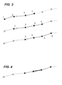
Fig. 2 depicts how a polynomial is calculated in accordance with the subject invention; -
Fig. 3 shows how six points create three cubic polynomials from four adjacent data points in accordance with the subject invention; -
Fig. 4 shows how the most accurate estimation is in the region bounded by the two centermost points that created the polynomial; -
Fig. 5 shows how four surrounding sets provide four valves of pressure and four valves of temperature in accordance with the subject invention; and -
Fig. 6 is a highly schematic block diagram showing the primary components associated with an example of a sensor in accordance with the subject invention. - Aside from the preferred embodiment or embodiments disclosed below, this invention is capable of other embodiments and of being practiced or being carried out in various ways. Thus, it is to be understood that the invention is not limited in its application to the details of construction and the arrangements of components set forth in the following description or illustrated in the drawings. If only one embodiment is described herein, the claims hereof are not to be limited to that embodiment. Moreover, the claims hereof are not to be read restrictively unless there is clear and convincing evidence manifesting a certain exclusion, restriction, or disclaimer.
- The subject invention uses simple interpolating polynomial functions that represents the function accurately over a narrow range in one dimension. The full range is achieved by providing sets of such polynomials. Two dimensional interpolation is then realized by creating several sets of polynomials which are then combined to form a unified representation of the data.
- Typically, calibration data points are collected from measurements taken to form grid of sensor characteristics in at least two variables. In one example, this would be the measurement of sensor frequency F and sensor temperature T at various applied pressures (Papplied) and test temperatures (Tapplied). For example, this might be at 9 pressures and 5 temperatures yielding 45 data points as shown in
Fig. 1 . There is no requirement for the grid to be either equally spaced nor contain equal number of points in each dimension. Indeed, it may be preferable to have a higher point density in areas of uncertainty. - Each of these points would have associated with them precisely measured values of P, F and T. The measured values of P and T may differ significantly from the applied values.
- Various means are used to fit an interpolating polynomial of order"n" to "n+1" data points. This solution is unique and the function exactly passes thru the calibration data points. For example, 4 points can be used to define the cubic polynomial shown in
Fig. 2 . - For each row in the point grid or
Fig. 1 , there are a set of points representing the function. Several "nth" order polynomials can be fitted to adjacent data points. If the number of points in the row is P, there will be p-n such polynomials. - In this example, each value of Tapplied will have 9 points (P, F, T) allowing a set of six cubic polynomial P=f(F) to be calculated for each value of Tapplied.
-
Fig. 3 shows how 6 points create 3 cubic polynomials from 4 adjacent points. - Since the polynomials overlap, they provide several estimates of the function. The most accurate estimation is in the region bounded by the two centermost points that created the polynomial as shown in
Fig. 4 . At the extremes of data, where no choice exists we use the nearest polynomial estimation can be used. - With this selection, there is now a method to provide an accurate estimation across the range bounded by the data points. There will be one such estimate for every row in the original data.
- The process is then repeated for the second variable. In the example, this would yield 6 polynomials T =f(F) for each value of Tapplied. The two polynomial sets above are created for all rows. So in the present example, this would give 5 sets, each containing 6 polynomials P=f(F) and 6 polynomials T =f(F).
- Calculation of these all polynomials (60 in this example) may present a severe challenge to both the computational power and accuracy that can be achieved in a simple sensor device. So, Newton's method can be used to solve these polynomials. This method accurately computes the Newtonian form of polynomial and can exploit the adjacent nature of the points to use "Newton's Triangle" to substantial reduce computational requirements and enhance accuracy.
- The polynomials may be pre-calculated and held in memory. Alternatively the defining data points alone may be held in memory and polynomial calculation delayed until it is needed. For the first method, there are two tables of 30 polynomials related to the row/column order of the original data points (instead of 9 x 5, there would be 6 x 5 i.e. 5 sets each containing 6 polynomials.)
- In the field where the pressure sensor is subjected to a pressure P at a temperature Tµ, the frequency of the transducer is Fµ. To evaluate the function P at any point FµTµ, the polynomial sets that surround the point are selected. Selection of these polynomials (or their defining points) is accomplished using a simple search of the data point table held in memory. For the unknowns Tµ and Fµ, the table of polynomials is searched to find the ones which surround the unknown. In the example, four are needed for a cubic fit so that is two on either side. For the second method, only the original data is stored. So, instead of finding the four polynomials which surround Tµ and Fµ, all the points which define those polynomials are located. This would be a collection of 16 points that surround Tµ and Fµ. A cubic function suits the variability of P with T, so for any given point the four nearest sets that surround that point are selected.
- Each of these sets of polynomials can now be evaluated to give P and T values for the given value of Fµ using a substitution in the pre-calculated Newtonian polynomials. Alternatively a combined interpolation and evaluation of the original data points using Lagrange's method can be employed. In this case, 16 original data points would be chosen, to create four polynomials.
- In our example, the four surrounding sets provide four values of P and four values of T for the given value Fµ as shown in
Fig. 5 . - These four new points define a cubic polynomial function P=f(T) which can then be evaluated at the given value of Tµ to provide final output P.
- As only one evaluation is needed for the final polynomial, it is advantageous to use Lagrange's method to combine both interpolation and evaluation operations. This has lower computational demands and higher accuracy than separately creating the polynomial and evaluating it.
- As has been shown, Lagrange and Newton's method can be used to substantially reduce the computational power required. Newton's method allows a pre-calculation of all the polynomials in an accurate and efficient manner leaving only the evaluation of m+1 of these polynomials and final interpolation using Lagrange's method.
- Alternatively, to conserve memory, just the original data points maybe be stored. Lagrange's method can then be used to combine both interpolation and evaluation.
-
Fig. 6 showspressure sensor 10 having an output P andtransducer 12 which generates a different frequency F when subject to different pressures.Temperature sensor 14 measures thetemperature T. Processor 16 is responsive to both F and T and is configured (e.g.) programmed to operate according to the method discussed above. EEPROM 18 (or some other memory) stores the values of F and P at different temperatures T as discussed above in reference toFig. 1 .Processor 16 outputs (to a display, for example) Pµ whentransducer 12 is subject to Pµ at temperature Tµ and exhibits a frequency Fµ. The above method has yielded accuracy of better than 1ppm using single precision floating point calculations. - But, the subject invention is not limited to pressure transducers and the method described above can be used with other types of sensors. Generally, it is assumed that data has been collected from test or calibration measurements. This data is of the form (X,Y,Z). For example, consider a test of a pressure sensor across a range of different applied pressures and temperatures. Z is the measured pressure, X is the temperature sensor measurement and Y is the output of the sensor.
- The following procedure will then accurately estimate the value of Z for any given value of X=x and Y=y, using a two dimensional polynomial function of order m x n.
- In step one, the data points (X,Y,Z) are arranged to represent a grid of Z values for two input variables X and Y where X and Y are in monotonic order. See
Fig. 1 . In step two, the (m+1) by (n+1) point matrix that spans the (x, y) point to be evaluated is selected. In step three, m+1 polynomials of order n using n+1 points where Z=f(Y) are solved. In step four, m+1 polynomials of order n using n+1 points where X=f(Y) are solved. In step five, the polynomials found in step four, are evaluated for the input value of Y=y to give m+1 values for Z and X. In step six, the polynomial of order m is solved using the m+1 data points for Z=f(X). Then, in step seven, Z is evaluated using the polynomial from step six for the input value of X=x. - Selecting the point matrix may be accomplished using a search of the data values. This search maybe optimized for efficiency using established methods.
- Steps three and four, solving the Z=f(Y) and X=f(Y) polynomials, may be optimized by pre-calculating the polynomials using the Newtonian form to preserve accuracy and calculation efficiency. Alternatively, these steps and the evaluation step may be combined using Lagrange's interpolation to reduce memory requirements and still maintains accuracy. The last two steps are preferably combined using Lagrange's interpolation and evaluation.
- The subject invention can be employed in a wide variety of sensor and control applications. For example, in engine control, it is common to take two measurements to derive a third parameter. For example, RPM and manifold pressure can be used to determine ignition timing. The method of this invention can be used in such an application and the original data might be based on experimental or modeled conditions and the output would not typically be an indicator but instead part of the overall system control function.
- Thus, although specific features of the invention are shown in some drawings and not in others, this is for convenience only as each feature may be combined with any or all of the other features in accordance with the invention. The words "including", "comprising", "having", and "with" as used herein are to be interpreted broadly and comprehensively and are not limited to any physical interconnection. Moreover, any embodiments disclosed in the subject application are not to be taken as the only possible embodiments. Other embodiments will occur to those skilled in the art and are within the following claims.
- In addition, any amendment presented during the prosecution of the patent application for this patent is not a disclaimer of any claim element presented in the application as filed: those skilled in the art cannot reasonably be expected to draft a claim that would literally encompass all possible equivalents, many equivalents will be unforeseeable at the time of the amendment and are beyond a fair interpretation of what is to be surrendered (if anything), the rationale underlying the amendment may bear no more than a tangential relation to many equivalents, and/or there are many other reasons the applicant can not be expected to describe certain insubstantial substitutes for any claim element amended.
Claims (12)
- A. method of sensing pressure, the method comprising:subjecting a pressure sensor having on output P which varies based on the sensor's frequency F and the temperature T to several different temperatures and applied pressures;determining the sensor's frequency F at the different temperatures and applied pressures and collecting data points representing the same;from the data points and at each different temperature, generating several polynomials P=f(F) and T=f(F);using the sensor to sense an unknown pressure Pµ at a temperature Tµ at which the sensor has a frequency Fµ;selecting, from the generated polynomials, polynomials that surround Tµ and Fµ;evaluating the selected polynomials for Fµ to calculate values for P=f(Fµ) and T=f(Fµ);from the calculated values, generating a polynomial P=f(T); andsolving Pµ=f(T) for Tµ and outputting Pµ.
- The method of claim 1, in which generating the polynomials includes employing Newton's method.
- The method of claim 1 or claim 2, in which the generated polynomials are stored.
- The method of any one of the preceding claims, in which the data points are stored and the polynomials are not generated until the surrounding data points are selected.
- The method of any one of the preceding claims, in which solving Pµ=f(T) includes using Lagrange's method.
- A pressure sensor comprising:a resonant pressure transducer whose frequency F changes depending on the applied pressure P and the temperature T;a temperature sensor for measuring the temperature T;a memory including stored therein data points corresponding to the sensor's frequency F at different applied pressures and temperatures; anda processor configured to:generate several polynomials P=f(F) and T=f(F) from the data points,calculate Pµ at Tµ when the transducer frequency is Fµ by:selecting, from the generated polynomials, polynomials that surround Fµ and Tµ,evaluating the selected polynomials for Fµ to calculate values for P=f(Fµ) and T=f(Fµ),generating a polynomial P=f(T) for the calculated values, andsolving Pµ=f(T) for Tµ, andoutput Pµ.
- A method of determining an unknown parameter Z based on two measured parameters X and Y, the method comprising:determining Z at different values of X and Y and collecting data points representing the same;from the data points, generating several polynomials Z=f(X) and X=f(Y);determining an unknown parameter Zµ at Xµ and Yµ;selecting, from the generated polynomials, polynomials that surround Xµ and Yµ;evaluating the selected polynomials for Yµ to calculate values for Z=f(Yµ) and X=f(Yµ);from the calculated values, generating a polynomial Z=f(X); andsolving Zµ=f(X) for Xµ and outputting Zµ.
- The method of claim 7, in which generating the polynomials includes employing Newton's method.
- The method of claim 7 or claim 8, in which the generated polynomials are stored.
- The method of any one of claims 7 to 9, in which the data points are stored and the polynomials are not generated until surrounding data points are selected.
- The method of claims 7 to 10, in which solving Zµ=f(X) includes using Lagrange's method.
- A sensor system comprising:a sensor with a parameter Y that changes depending on parameter Z and parameter X;a device which measures parameter X;a memory including stored therein data points corresponding to values of parameter Y at different values of Z and X; anda processor configured to:general several polynomials Z=f(X) and X=f(Y) from the data points,calculate Zµ at Xµ when the sensor measures Yµ by:output Zµ.selecting, from the generated polynomials, polynomials that surround Yµ and Xµ,evaluating the selected polynomials for Yµ to calculate values for Z=f(Yµ) and X=f(Yµ),generating a polynomial Z=f(X) for the calculated values, andsolving Zµ=f(X) for Xµ, and
Applications Claiming Priority (1)
| Application Number | Priority Date | Filing Date | Title |
|---|---|---|---|
| US12/130,977 US7783448B2 (en) | 2008-05-30 | 2008-05-30 | Sensor processing method |
Publications (2)
| Publication Number | Publication Date |
|---|---|
| EP2128584A2 true EP2128584A2 (en) | 2009-12-02 |
| EP2128584A3 EP2128584A3 (en) | 2015-01-14 |
Family
ID=40999973
Family Applications (1)
| Application Number | Title | Priority Date | Filing Date |
|---|---|---|---|
| EP09160941.2A Withdrawn EP2128584A3 (en) | 2008-05-30 | 2009-05-22 | Pressure sensor calibration method |
Country Status (5)
| Country | Link |
|---|---|
| US (1) | US7783448B2 (en) |
| EP (1) | EP2128584A3 (en) |
| JP (1) | JP5624285B2 (en) |
| KR (1) | KR101483309B1 (en) |
| CN (1) | CN101592540B (en) |
Cited By (2)
| Publication number | Priority date | Publication date | Assignee | Title |
|---|---|---|---|---|
| WO2014160912A3 (en) * | 2013-03-29 | 2015-01-08 | Dresser, Inc. | Temperature compensated pressure transducer |
| EP2817602A4 (en) * | 2012-02-21 | 2015-12-02 | Dresser Inc | PRESSURE TRANSDUCER CORRECTED IN TEMPERATURE |
Families Citing this family (12)
| Publication number | Priority date | Publication date | Assignee | Title |
|---|---|---|---|---|
| EP2189774B1 (en) * | 2008-11-20 | 2014-12-31 | VEGA Grieshaber KG | Method of detecting and compensating for a quick temperature change to a pressure measurement cell |
| JP2012216963A (en) * | 2011-03-31 | 2012-11-08 | Mitsumi Electric Co Ltd | Function generation circuit, control signal generation method, and curve fitting method |
| US20130218502A1 (en) * | 2012-02-21 | 2013-08-22 | Dresser, Inc. | Temperature compensated pressure transducer |
| CN104568289A (en) * | 2013-10-23 | 2015-04-29 | 北京临近空间飞行器系统工程研究所 | Pressure Generation Method Based on Silicon Resonant Sensor |
| CN103712741B (en) * | 2013-11-15 | 2016-01-20 | 上海新干通通信设备有限公司 | The bearing calibration of line pressure sensor |
| CN104535251B (en) * | 2015-01-12 | 2017-02-22 | 中国科学院电子学研究所 | Temperature self-compensating method and measuring mode for double-resonator pressure sensor |
| US10324004B2 (en) * | 2015-04-15 | 2019-06-18 | The Boeing Company | Methods and devices for adaptive autonomous polynomial interpolation of time series data |
| CN108593203B (en) * | 2018-04-28 | 2019-08-09 | 福州大学 | Calibration method of pressure sensor based on MC8051 |
| CN110823335B (en) * | 2018-08-10 | 2021-06-25 | 张德贤 | Grain silo detection method and system based on bottom surface single-circle standard deviation polynomial model |
| CN114323430B (en) * | 2021-12-30 | 2024-09-17 | 杭州和利时自动化有限公司 | Temperature compensation method, system and device for pressure transmitter and storage medium |
| US11714015B1 (en) * | 2022-03-29 | 2023-08-01 | Rosemount Aerospace Inc. | Method for thermoelectric effect error correction |
| CN118625856A (en) * | 2024-04-26 | 2024-09-10 | 华能伊敏煤电有限责任公司 | A mine car operation management method and system based on Internet control |
Family Cites Families (17)
| Publication number | Priority date | Publication date | Assignee | Title |
|---|---|---|---|---|
| US4644482A (en) * | 1984-12-21 | 1987-02-17 | Pressure Systems Incorporated | Digital pressure transducer and corrections circuitry system |
| JPS63281033A (en) * | 1987-05-13 | 1988-11-17 | Daiwa Shinku Kogyosho:Kk | Pressure detector |
| JPH02232541A (en) * | 1989-03-06 | 1990-09-14 | Shimadzu Corp | Pressure measuring apparatus |
| JPH03243840A (en) * | 1990-02-21 | 1991-10-30 | Daishinku Co | Temperature compensation method of piezoelectric vibrator pressure sensor |
| US5497665A (en) * | 1991-02-05 | 1996-03-12 | Direct Measurement Corporation | Coriolis mass flow rate meter having adjustable pressure and density sensitivity |
| US5329818A (en) * | 1992-05-28 | 1994-07-19 | Rosemount Inc. | Correction of a pressure indication in a pressure transducer due to variations of an environmental condition |
| JPH06137977A (en) * | 1992-10-29 | 1994-05-20 | Vacuum Prod Kk | Method for measuring pressure using quartz oscillator |
| US5500509A (en) * | 1994-03-01 | 1996-03-19 | Borg-Warner Automotive, Inc. | Microprocessor based universal digital pressure sensor |
| JPH08201189A (en) * | 1995-01-24 | 1996-08-09 | Hitachi Ltd | Compensation method for electronic measuring device |
| US5551301A (en) | 1995-06-19 | 1996-09-03 | Cardiometrics, Inc. | Piezoresistive pressure transducer circuitry accommodating transducer variability |
| DE19531926C2 (en) * | 1995-08-16 | 1998-05-28 | Hartmann & Braun Ag | Method for correcting a differential pressure signal |
| US6170338B1 (en) * | 1997-03-27 | 2001-01-09 | Rosemont Inc. | Vortex flowmeter with signal processing |
| JP2000019039A (en) | 1998-07-03 | 2000-01-21 | Ishikawajima Harima Heavy Ind Co Ltd | Pressure transducer |
| US6935156B2 (en) * | 2003-09-30 | 2005-08-30 | Rosemount Inc. | Characterization of process pressure sensor |
| US7124047B2 (en) * | 2004-09-03 | 2006-10-17 | Eaton Corporation | Mathematical model useful for determining and calibrating output of a linear sensor |
| ES2353768T3 (en) * | 2004-11-17 | 2011-03-04 | Volvo Lastvagnar Ab | PROCEDURE FOR THE DETERMINATION OF A MIDDLE MOTOR TORQUE. |
| US20060176048A1 (en) * | 2005-02-07 | 2006-08-10 | Zhengrong Zhou | Generation and use of calibration data for automated test equipment |
-
2008
- 2008-05-30 US US12/130,977 patent/US7783448B2/en active Active
-
2009
- 2009-05-22 EP EP09160941.2A patent/EP2128584A3/en not_active Withdrawn
- 2009-05-26 CN CN200910141817.XA patent/CN101592540B/en active Active
- 2009-05-28 JP JP2009128374A patent/JP5624285B2/en active Active
- 2009-05-28 KR KR20090046966A patent/KR101483309B1/en active Active
Non-Patent Citations (1)
| Title |
|---|
| LAYHOU ET AL.: "A Noniterative Polynomial 2-D Calibration Method Implemented in a Microcontroller", IEEE TRANSACTIONS ON INSTRUMENTATION AND MEASUREMENT, vol. 46, no. 4, 1 August 1997 (1997-08-01), pages 752, XP055250250 * |
Cited By (2)
| Publication number | Priority date | Publication date | Assignee | Title |
|---|---|---|---|---|
| EP2817602A4 (en) * | 2012-02-21 | 2015-12-02 | Dresser Inc | PRESSURE TRANSDUCER CORRECTED IN TEMPERATURE |
| WO2014160912A3 (en) * | 2013-03-29 | 2015-01-08 | Dresser, Inc. | Temperature compensated pressure transducer |
Also Published As
| Publication number | Publication date |
|---|---|
| JP5624285B2 (en) | 2014-11-12 |
| CN101592540A (en) | 2009-12-02 |
| CN101592540B (en) | 2014-03-26 |
| KR20090124972A (en) | 2009-12-03 |
| JP2009288244A (en) | 2009-12-10 |
| EP2128584A3 (en) | 2015-01-14 |
| KR101483309B1 (en) | 2015-01-15 |
| US7783448B2 (en) | 2010-08-24 |
| US20090299658A1 (en) | 2009-12-03 |
Similar Documents
| Publication | Publication Date | Title |
|---|---|---|
| US7783448B2 (en) | Sensor processing method | |
| US5965824A (en) | Vibration type measuring instrument | |
| EP3218747B1 (en) | Optical fiber and method and apparatus for accurate fiber optic sensing under multiple stimuli | |
| CN103162901A (en) | Nonlinear calibrating method for multiple temperature points of pressure sensor | |
| US20090216477A1 (en) | Measuring apparatuses and methods of using them | |
| US20090299657A1 (en) | Air flow measurement device and air flow correction method | |
| EP1150103B1 (en) | Method of setting flow coefficient and flow meter | |
| JP4810876B2 (en) | Bolt axial force measuring device | |
| US7100450B2 (en) | Method for correcting pressure measurement for the influence of temperature in a sapphire gauge | |
| CN114689214B (en) | Temperature sensor testing equipment and temperature sensor compensation method | |
| US6668236B1 (en) | Process for calibrating a sensor for measuring an angle of inclination of a motor vehicle wheel | |
| US20010044703A1 (en) | Calculation device and method therefor | |
| CN117664253A (en) | Compensation method for measuring precision of ultrasonic flowmeter and control device thereof | |
| CN119666094B (en) | A temperature-adaptive ultrasonic flow measurement method and system | |
| Yadav et al. | Evaluation of associated uncertainties in calibration of direct pressure indicating electromechanical devices | |
| JP2004028653A (en) | Internal diameter measuring device | |
| JP7716914B2 (en) | Offset estimation device and offset estimation method | |
| Klevtsov | Plane Conversion Characteristic Model for Microprocessor Pressure Sensor | |
| JP5259950B2 (en) | Processing device for exhaust gas analysis and exhaust gas analysis method | |
| WO2024162135A1 (en) | Virtual flow rate computing apparatus, virtual flow rate computing method, and virtual flow rate computing program | |
| RU2503968C1 (en) | Method to correct characteristics of measuring converters | |
| RU2504760C2 (en) | Method of measurement for gaseous media polycomposition | |
| Dyurish et al. | A matrix interpretation of the estimate of the extension of uncertainties when constructing a temperature scale | |
| DeLoach et al. | A Statistical Theory of Bidirectionality | |
| JPH08304104A (en) | Compensation method for electronic measuring device |
Legal Events
| Date | Code | Title | Description |
|---|---|---|---|
| PUAI | Public reference made under article 153(3) epc to a published international application that has entered the european phase |
Free format text: ORIGINAL CODE: 0009012 |
|
| AK | Designated contracting states |
Kind code of ref document: A2 Designated state(s): AT BE BG CH CY CZ DE DK EE ES FI FR GB GR HR HU IE IS IT LI LT LU LV MC MK MT NL NO PL PT RO SE SI SK TR |
|
| PUAL | Search report despatched |
Free format text: ORIGINAL CODE: 0009013 |
|
| AK | Designated contracting states |
Kind code of ref document: A3 Designated state(s): AT BE BG CH CY CZ DE DK EE ES FI FR GB GR HR HU IE IS IT LI LT LU LV MC MK MT NL NO PL PT RO SE SI SK TR |
|
| RIC1 | Information provided on ipc code assigned before grant |
Ipc: G01L 27/00 20060101AFI20141208BHEP |
|
| 17P | Request for examination filed |
Effective date: 20150714 |
|
| RBV | Designated contracting states (corrected) |
Designated state(s): AT BE BG CH CY CZ DE DK EE ES FI FR GB GR HR HU IE IS IT LI LT LU LV MC MK MT NL NO PL PT RO SE SI SK TR |
|
| 17Q | First examination report despatched |
Effective date: 20150909 |
|
| STAA | Information on the status of an ep patent application or granted ep patent |
Free format text: STATUS: THE APPLICATION IS DEEMED TO BE WITHDRAWN |
|
| 18D | Application deemed to be withdrawn |
Effective date: 20161201 |