EP1995575A2 - System for analysing the frequency of resonant devices - Google Patents
System for analysing the frequency of resonant devices Download PDFInfo
- Publication number
- EP1995575A2 EP1995575A2 EP08156845A EP08156845A EP1995575A2 EP 1995575 A2 EP1995575 A2 EP 1995575A2 EP 08156845 A EP08156845 A EP 08156845A EP 08156845 A EP08156845 A EP 08156845A EP 1995575 A2 EP1995575 A2 EP 1995575A2
- Authority
- EP
- European Patent Office
- Prior art keywords
- function
- square
- representative
- analysis system
- frequency
- Prior art date
- Legal status (The legal status is an assumption and is not a legal conclusion. Google has not performed a legal analysis and makes no representation as to the accuracy of the status listed.)
- Granted
Links
- 238000005259 measurement Methods 0.000 claims abstract description 7
- 230000010349 pulsation Effects 0.000 claims description 16
- 230000010355 oscillation Effects 0.000 claims description 7
- 238000005070 sampling Methods 0.000 claims description 4
- 238000013016 damping Methods 0.000 claims description 3
- 230000010287 polarization Effects 0.000 claims 1
- 230000001133 acceleration Effects 0.000 description 48
- 238000004422 calculation algorithm Methods 0.000 description 13
- 238000001228 spectrum Methods 0.000 description 11
- 241000897276 Termes Species 0.000 description 8
- 230000005284 excitation Effects 0.000 description 7
- 238000012545 processing Methods 0.000 description 6
- 238000000034 method Methods 0.000 description 4
- 230000003595 spectral effect Effects 0.000 description 4
- 238000011161 development Methods 0.000 description 3
- 238000010586 diagram Methods 0.000 description 3
- 101100042630 Caenorhabditis elegans sin-3 gene Proteins 0.000 description 2
- 238000004364 calculation method Methods 0.000 description 2
- 230000003111 delayed effect Effects 0.000 description 2
- 238000001514 detection method Methods 0.000 description 2
- 230000000694 effects Effects 0.000 description 2
- 230000003071 parasitic effect Effects 0.000 description 2
- 230000010363 phase shift Effects 0.000 description 2
- 230000001360 synchronised effect Effects 0.000 description 2
- 238000012546 transfer Methods 0.000 description 2
- 241001644893 Entandrophragma utile Species 0.000 description 1
- 230000008602 contraction Effects 0.000 description 1
- 230000001419 dependent effect Effects 0.000 description 1
- 238000009795 derivation Methods 0.000 description 1
- 229940082150 encore Drugs 0.000 description 1
- 239000000284 extract Substances 0.000 description 1
- 238000001914 filtration Methods 0.000 description 1
- 238000009472 formulation Methods 0.000 description 1
- 230000000670 limiting effect Effects 0.000 description 1
- 239000000203 mixture Substances 0.000 description 1
- 230000002829 reductive effect Effects 0.000 description 1
- 230000000284 resting effect Effects 0.000 description 1
- 230000003068 static effect Effects 0.000 description 1
- 230000036962 time dependent Effects 0.000 description 1
- 238000013519 translation Methods 0.000 description 1
Images


Classifications
-
- G—PHYSICS
- G01—MEASURING; TESTING
- G01H—MEASUREMENT OF MECHANICAL VIBRATIONS OR ULTRASONIC, SONIC OR INFRASONIC WAVES
- G01H13/00—Measuring resonant frequency
-
- G—PHYSICS
- G01—MEASURING; TESTING
- G01P—MEASURING LINEAR OR ANGULAR SPEED, ACCELERATION, DECELERATION, OR SHOCK; INDICATING PRESENCE, ABSENCE, OR DIRECTION, OF MOVEMENT
- G01P15/00—Measuring acceleration; Measuring deceleration; Measuring shock, i.e. sudden change of acceleration
- G01P15/02—Measuring acceleration; Measuring deceleration; Measuring shock, i.e. sudden change of acceleration by making use of inertia forces using solid seismic masses
- G01P15/08—Measuring acceleration; Measuring deceleration; Measuring shock, i.e. sudden change of acceleration by making use of inertia forces using solid seismic masses with conversion into electric or magnetic values
- G01P15/097—Measuring acceleration; Measuring deceleration; Measuring shock, i.e. sudden change of acceleration by making use of inertia forces using solid seismic masses with conversion into electric or magnetic values by vibratory elements
Definitions
- the field of the invention is that of resonant or vibrating devices. It is known that the measurement principle of a large number of sensors is based on the measurement of the oscillation frequency of a mechanical system oscillating either in free oscillations or in forced oscillations, this frequency depending on the parameter that is sought. to measure.
- vibrating-bar accelerometers also called VBAs used for the measurement of accelerations, it being understood that the following can easily be generalized to any vibrating system.
- FIG. 1 a schematic diagram of an accelerometer of this type. It essentially comprises a mass connected to two identical and parallel tuning fork beams 1, each beam carries two electrodes 2 and 3, the first electrode 2 serving for excitation and the second electrode 3 for detecting. Under the effect of an acceleration along the sensitive x-axis of the accelerometer, the mass moves in translation along this sensitive axis causing an extension or a contraction of the tuning fork and thus modifying its resonance frequency according to the relation 0 below.
- the principle of measuring the frequency is as follows.
- the excitation and vibration of the beams are maintained by the excitation electrode 2 covering part of the length of each beam.
- the excitation voltage is the sum of a DC voltage V 0 and an AC voltage v at the resonant frequency of the oscillator, created by loopback of the output signal of the sensor.
- the rest of the surface of the two beams is covered by a detection electrode 3 biased at the voltage V 0 .
- the vibration movement of the beams varying the distance between the beams and this electrode, a detection current appears in the electrode.
- This current flows into a charge amplifier filter.
- the voltage at the output of this filter is the output signal of the sensor.
- This output signal is used on the one hand for the processing 6 making it possible to recover, from the resonance frequency measurement, the acceleration applied to the sensor and, on the other hand, as input into the loopback 4 making it possible to generate the voltage alternative of excitement.
- the acceleration applied to the sensor From the signals returned by the accelerometer, we must find the acceleration applied to the sensor.
- the non-linear nature of the relationship 0 poses a fundamental problem. Indeed, the acceleration a in relation 0 contains not only the useful acceleration applied to the sensor but also vibration terms that can reach very high values.
- the mass-spring system formed by the mass and the resonator has a resonance frequency f R. At this frequency, the noises are greatly amplified.
- the acceleration applied to the sensor comprises a low frequency term whose band is typically comprised of an interval varying from 0 Hz to 400 Hz which is the static or dynamic acceleration that it is desired to determine by virtue of the processing and a term centered on the frequency f R which is typically between 3 kHz and 5 kHz which corresponds to the noise filtered by the mass-spring system and which forms parasitic vibrations likely to degrade the results of the treatment.
- f R typically between 3 kHz and 5 kHz which corresponds to the noise filtered by the mass-spring system and which forms parasitic vibrations likely to degrade the results of the treatment.
- the movement of the beams can be represented by an equivalent one-dimensional oscillator according to the direction and direction of the sensitive axis of the sensor.
- This acceleration includes both the term low frequency that is sought to measure and high frequency terms due to vibrations, ⁇ i : nonlinearity coefficient of order 3, e (t): excitation term, function of time.
- ⁇ 0 1 + at ⁇ VS is the resonant pulse of the vibrating system subjected to acceleration a.
- the current in the sensing electrode is proportional to the speed of the equivalent oscillator.
- the transfer function of the charge amplifier filter is that of an integrator.
- the output voltage of the charge amplifier is obtained by integrating the speed of the equivalent oscillator. If the signal corresponding to the position of the oscillator has a low frequency term, this term is not found at the output of the charge amplifier. The output voltage of the charge amplifier is then proportional to the high frequency terms of the oscillator position signal.
- a first method consists in considering that the frequency of the output signal of the sensor denoted f is related to the acceleration by the relation f ⁇ f 0 ⁇ 1 + at ⁇ VS .
- f 1 and f 2 the frequencies of the output signals on channels 1 and 2 and making a limited development of said frequencies, the following relationships are obtained: f 1 ⁇ f 0 , 1 ⁇ 1 + at ⁇ VS , 1 ⁇ f 0 , 1 ⁇ 1 + at 2 ⁇ ⁇ VS , 1 - at 2 8 ⁇ ⁇ VS , 1 2 + at 3 16 ⁇ ⁇ VS , 1 3 + ...
- Another method is to determine the acceleration from the difference of the square of the frequencies. This method is described in the French patent reference FR 2 590 991 .
- the frequency of the sensor output signal is assumed to be related to acceleration by the following relationships, with the same notations as before: f I , 1 ⁇ f 0 , 1 ⁇ 1 + at 0 + ⁇ V , 1 ⁇ cos 2 ⁇ ⁇ f R ⁇ t ⁇ VS , 1 f I , 2 ⁇ f 0 , 2 ⁇ 1 + at 0 + ⁇ V , 2 ⁇ cos 2 ⁇ ⁇ f R ⁇ t ⁇ VS , 2
- the device that extracts the frequencies in the form of a transfer function having a unity gain and a zero phase shift for the low frequencies, a gain ⁇ and a phase shift ⁇ for the frequency f R and a zero gain for the multiple frequencies of f R.
- This device can be, for example, a PLL, acronym for Phase-Locked Loop, which means phase locked loop.
- f i , 1 f 0 , 1 1 + at 0 + ⁇ V , 1 ⁇ cos 2 ⁇ ⁇ f R ⁇ t 2 ⁇ ⁇ VS , 1 - at 0 2 + ⁇ V , 1 2 ⁇ cos 2 2 ⁇ ⁇ f R ⁇ t + 2 ⁇ at 0 + ⁇ V , 1 ⁇ cos 2 ⁇ ⁇ f R ⁇ t 8 ⁇ VS , 1 2 + 1 16 ⁇ ⁇ VS , 1 3 ⁇ at 0 3 + ⁇ V , 1 3 ⁇ cos 3 2 ⁇ ⁇ f R ⁇ t + 3 ⁇ at 0 ⁇ ⁇ V , 1 2 ⁇ cos 2 2 ⁇ ⁇ f R ⁇ t + 3 ⁇ at 0 2 ⁇ ⁇ V , 1 ⁇ cos 2 ⁇ ⁇ f R ⁇ t + 3 ⁇ at 0 2 ⁇ ⁇ V , 1 ⁇ cos 2 ⁇ ⁇ f R ⁇
- f s , 1 f 0 , 1 1 + at 0 + ⁇ ⁇ ⁇ V , 1 ⁇ cos 2 ⁇ ⁇ f R ⁇ t + ⁇ 2 ⁇ ⁇ VS , 1 - at 0 2 + ⁇ V , 1 2 / 2 + 2 ⁇ at 0 + ⁇ V , 1 ⁇ ⁇ cos ⁇ 2 ⁇ ⁇ f R ⁇ t + ⁇ 8 ⁇ VS , 1 2 + 1 16 ⁇ ⁇ VS , 1 3 ⁇ at 0 3 + ⁇ V , 1 3 ⁇ 3 4 ⁇ ⁇ cos ⁇ 2 ⁇ ⁇ f R ⁇ t + ⁇ + 3 ⁇ at 0 ⁇ ⁇ V , 1 2 2 + 3 ⁇ at 0 2 ⁇ ⁇ V , 1 ⁇ ⁇ cos ⁇ 2 ⁇ ⁇ f R ⁇ t + ⁇ and f s
- f S , 1 2 - f 0 , 1 2 f 0 , 2 2 ⁇ f S , 2 2 f 0 , 1 2 at 0 ⁇ 1 ⁇ VS , 1 + 1 ⁇ VS , 2 + ⁇ 2 - 1 8 ⁇ ⁇ V , 1 2 ⁇ VS , 1 2 - ⁇ V , 2 2 ⁇ VS , 2 2 + at 0 ( 1 - ⁇ 2 ) 8 ⁇ ⁇ V , 1 2 ⁇ VS , 1 3 + ⁇ V , 2 2 ⁇ VS , 2 3
- the system according to the invention does not have the above disadvantages. It is known that the spectrum of the output signal is centered on the frequency f a0 equal to the sum of the central frequency of the resonator and a deviation due to the low frequency acceleration a 0 applied to the sensor. This spectrum comprises lines located at frequencies f a0 ⁇ kf R due to vibrations.
- the system according to the invention implements an algorithm performing a broadband demodulation of the output signal of the sensor, taking into account the lines of significant amplitude. The algorithm is based on rigorous theoretical relationships between the acceleration-induced stiffness variation and the characteristic parameters of the sensor output signal, which are the instantaneous amplitude and the instantaneous frequency.
- the spectrum of the output signal contains lines at frequencies below f R.
- these lines are of negligible amplitudes.
- the sampling frequency must be high enough to contain the signal spectrum. For example, with the modulation indices and frequencies involved for accelerometers at resting resonant frequency and vibration, the order of magnitude of the sampling frequency should be 250 kHz.
- the subject of the invention is a system for analyzing the oscillation frequency of a vibrating device along an axis, the said system comprising means for measuring the position A of the device along this axis, the signal coming from said means representative of the position A being represented by a time dependent function U, characterized in that said system comprises first means for calculating the function ⁇ 1 2 - ⁇ 1 2 ⁇ 1 , ⁇ 1 being the instantaneous pulsation of U, ⁇ 1 its instantaneous amplitude and ⁇ 1 (2) the second derivative of said instantaneous amplitude, the function ⁇ 1 2 - ⁇ 1 2 ⁇ 1 being representative of the square of the resonance pulse ⁇ of the vibrating device.
- said first means comprise means for calculating the second derivative of the function U denoted by U (2) , of the Hilbert transform of the function U denoted V, of the second derivative of this Hilbert transform denoted V (2). as well as a first function equal to U . U 2 + V . V 2 U 2 + V 2 mathematically equal to ⁇ 1 2 - ⁇ 1 2 ⁇ 1 , representative of the square of the resonance pulse ⁇ of the vibrating device.
- said device when the differential equation representative of the variations of position A of the device comprises non-linear order 3 terms, said device then comprises second means for performing, using the preceding notations, a second function equal to V 2 ⁇ V + U 2 ⁇ U U 2 + V 2 - ⁇ i ⁇ 3 4 ⁇ K 1 2 ⁇ U 2 + V 2 , representative of the square of the resonance pulse n of the vibrating device, ⁇ i and K 1 being constants.
- the vibrating device when the vibrating device is forced oscillation, that is to say that the device comprises a phase and amplitude control arranged to eliminate the natural damping of the device, said servocontrol generating a bias V 0 , said device then comprises third means for performing, using the preceding notations, a third function equal to V 2 ⁇ V + U 2 ⁇ U U 2 + V 2 - ⁇ i ⁇ 3 4 ⁇ K 1 2 ⁇ U 2 + V 2 + 3 ( K 3 ⁇ V 0 2 - UU 2 + VV 2 U 2 + V 2 ⁇ ) 2 , Representative the square of the resonance pulse ⁇ of the vibrating device, ⁇ i , K 1 and K 3 being constants.
- the analysis system is an electronic system, the function U being an electrical parameter, said system comprising means for digitizing and sampling the function U, first filters with finite impulse response capable of producing the Hilbert transform. an electronic function, second finite impulse response filters adapted to perform the derivative of an electrical function, delay lines for synchronizing the various sampled signals, electronic means performing the summation, multiplication and division functions; and notch filters and low-pass filters.
- the core of the invention is based on an algorithm performing broadband demodulation of the output signal of the sensor.
- This algorithm implements Hilbert transforms and their properties.
- x ( t ) be a real signal
- ⁇ ⁇ 0 + ⁇ v cos (2 ⁇ f R t ) a 0 representing the useful low frequency part of the acceleration applied to the sensor and ⁇ v being a constant representing the amplitude of the vibrations.
- I A 1 and we denote Q the Hilbert transform of I.
- the output voltage U 1 of the charge amplifier is proportional to the signal I.
- the spectrum of the position signal of the oscillator does not include a low frequency term.
- each rectangle represents an electronic element ensuring a particular function.
- the Hilbert transform V 1 is obtained by means of a finite impulse response filter denoted FIR TH at N + 1 points whose spectral band includes the lines of significant amplitude of the signal U 1 .
- the derivatives of the signals are calculated by a finite impulse response filter denoted FIR D at L + 1 points whose spectral band also includes these lines.
- the signal U 1 must be delayed by NOT 2 points to be synchronized with the signal V 1 by delay lines denoted R (N / 2). Then the signals U 1 and V 1 must be delayed by other delay lines denoted R (L) of L points to be synchronous with U 1 2 and V 1 2 . .
- This provides a broadband demodulation of the signal.
- the use of the algorithm using the second derivative and the Hilbert transform with filters having a sufficiently large bandwidth makes it possible to carry out broadband demodulation of the signal.
- the use of this algorithm is applicable to any dynamic system whose behavior is governed by a law of the type of the relation 0.
- the application of this algorithm to the accelerometer VBA without non-linearity of order 3 makes it possible to obtain a information of the instantaneous acceleration with the useful component and the vibrations.
- the useful component can be extracted by low-pass filtering.
- excitation e 1 K 4.1 ( V 0 + v ) 2 + K 5.1 V 0 2
- V 0 DC bias voltage
- ⁇ variable voltage obtained from a phase and amplitude feedback on the output voltage of the charge amplifier representing the output signal of the sensor.
- the voltage ⁇ is therefore at the frequency of the resonator.
- ⁇ 2 has a component at twice the resonance frequency that does not significantly affect the equation and a negligible continuous term with respect to the square of the DC bias voltage.
- I is a high frequency signal whose spectrum is centered on f ⁇ 0.1 .
- ⁇ is a low frequency signal. It has lines at f R , 2 f R ... due to the presence of the vibrations in a, but these lines are of negligible amplitude. So we have d 2 ⁇ I + ⁇ d t 2 ⁇ d 2 ⁇ I d t 2
- equation (8) is decomposed into a high frequency term and a low frequency term defined by K 3 , 1 ⁇ V 0 2 ⁇ 0 , 1 2 ⁇ 1 + at ⁇ VS , 1
- ⁇ I , ⁇ 3 I and K 3 , 1 ⁇ V 0 2 ⁇ I are high frequency terms. If we took them into account in the algorithm, they would in any case be eliminated by the low-pass filter placed at the end of the processing to isolate the useful part of the acceleration at low frequencies.
- I 2 + Q 2 2 3 4 ⁇ ⁇ 2 + ⁇ 2 4 ⁇ cos 2 ⁇ ⁇ .
- ⁇ 2 cos (2 ⁇ ) is also not in the useful frequency band.
- the information ⁇ having a low frequency spectrum is not present at the output of the charge amplifier.
- ⁇ 1 2 V 1 2 ⁇ V 1 + U 1 2 ⁇ U 1 U 1 2 + V 1 2 - ⁇ i , 1 ⁇ 3 4 ⁇ K 1 2 ⁇ U 1 2 + V 1 2 + 3 ( K 3 , 1 ⁇ V 0 2 - U 1 ⁇ U 1 2 + V 1 ⁇ V 1 2 U 1 2 + V 1 2 ⁇ ) 2 ,
- This function can be calculated by performing the function - V 1 2 ⁇ V 1 + U 1 2 ⁇ U 1 U 1 2 + V 1 2 - ⁇ i , 1 ⁇ 3 4 ⁇ K 1 2 ⁇ U 1 2 + V 1 2 + 3 ( K 3 , 1 ⁇ V 0 2 - U 1 ⁇ U 1 2 + V 1 ⁇ V 1 2 U 1 2 + V 1 2 ⁇ ) 2
- the acceleration estimated by this algorithm does not contain any significant bias introduced by the vibrations.
- the information returned by the algorithm varies linearly as a function of the acceleration applied to the sensor.
- the estimated acceleration of the relation 16 then comprises the useful part and the vibration terms.
- the ratios ⁇ 0 , 1 2 ⁇ 0 , 2 2 ⁇ ⁇ VS , 2 ⁇ VS , 1 and ⁇ 0 , 1 2 ⁇ 0 , 2 2 are temperature independent and can also be calibrated.
- the weighted sum of the two pieces of information therefore theoretically depends only on the temperature and does not depend on the acceleration. Thanks to the weighted sum of ⁇ 1 2 and of ⁇ 2 2 from relationship 17, it is thus possible to estimate the temperature and then to determine the acceleration thanks to the relation 16.
- the weighted difference thus makes it possible to overcome the error of bias due to a poor estimation of the temperature.
- the coefficients ⁇ i and ⁇ i are known by calibration. Informations ⁇ 1 2 and ⁇ 2 2 , we can therefore deduce the useful acceleration and the temperature.
- the differential treatment is represented in FIG. 4.
- the sum and the weighted difference are filtered by a cross-sectional filter denoted F.C.B. centered on the frequency of the vibrations and by a low pass filter noted F.P.B.
- F.C.B a cross-sectional filter centered on the frequency of the vibrations
- F.P.B a low pass filter
Abstract
Description
Le domaine de l'invention est celui des dispositifs résonnants ou vibrants. On sait que le principe de mesure d'un grand nombre de capteurs est basé sur la mesure de la fréquence des oscillations d'un système mécanique oscillant soit en oscillations libres, soit en oscillations forcées, cette fréquence dépendant du paramètre que l'on cherche à mesurer. On peut citer, à titre d'exemple, les accéléromètres à barreau vibrant encore appelés VBA utilisés pour la mesure des accélérations, étant entendu que ce qui suit peut se généraliser aisément à tout système vibrant.The field of the invention is that of resonant or vibrating devices. It is known that the measurement principle of a large number of sensors is based on the measurement of the oscillation frequency of a mechanical system oscillating either in free oscillations or in forced oscillations, this frequency depending on the parameter that is sought. to measure. By way of example, mention may be made of vibrating-bar accelerometers, also called VBAs used for the measurement of accelerations, it being understood that the following can easily be generalized to any vibrating system.
On trouvera en 
avec fa: fréquence de résonance de l'accéléromètre soumis à l'accélération,
f0 : fréquence de résonance du capteur au repos, c'est-à-dire soumis à une accélération d'entrée nulle,
a : accélération appliquée au capteur,
γc : accélération critique de flambage, paramètre physique du résonateur.We will find
with f a : resonance frequency of the accelerometer subjected to acceleration,
f 0: resonance frequency of the sensor at rest, that is to say subjected to a zero input acceleration,
a: acceleration applied to the sensor,
γ c : critical acceleration of buckling, physical parameter of the resonator.
Le principe de mesure de la fréquence est le suivant. L'excitation et la vibration des poutres sont entretenues par l'électrode d'excitation 2 couvrant une partie de la longueur de chaque poutre. La tension d'excitation est la somme d'une tension continue V0 et d'une tension alternative v à la fréquence de résonance de l'oscillateur, créée par rebouclage du signal de sortie du capteur. Le reste de la surface des deux poutres est couvert par une électrode de détection 3 polarisée à la tension V0. Le mouvement de vibration des poutres faisant varier la distance entre les poutres et cette électrode, un courant de détection apparaît dans l'électrode. Ce courant passe dans un filtre 5 amplificateur de charge. La tension à la sortie de ce filtre constitue le signal de sortie du capteur. Ce signal de sortie est utilisé d'une part pour le traitement 6 permettant de retrouver, à partir de la mesure de fréquence de résonance, l'accélération appliquée au capteur et d'autre part comme entrée dans le rebouclage 4 permettant de générer la tension alternative d'excitation.The principle of measuring the frequency is as follows. The excitation and vibration of the beams are maintained by the
A partir des signaux renvoyés par l'accéléromètre, on doit retrouver l'accélération appliquée au capteur. La nature non linéaire de la relation 0 pose un problème fondamental. En effet, l'accélération a dans la relation 0 contient non seulement l'accélération utile appliquée au capteur mais également des termes de vibration pouvant atteindre des valeurs très élevées. Le système masse-ressort formé par la masse et le résonateur présente une fréquence de résonance fR. A cette fréquence, les bruits sont fortement amplifiés. L'accélération appliquée au capteur comporte un terme basse fréquence dont la bande est typiquement comprise sur un intervalle variant de 0 Hz à 400 Hz qui est l'accélération statique ou dynamique que l'on souhaite déterminer grâce au traitement et un terme centré sur la fréquence fR qui est typiquement comprise entre 3 kHz et 5 kHz qui correspond au bruit filtré par le système masse-ressort et qui forme des vibrations parasites susceptibles de dégrader les résultats du traitement. Ces termes entraînent à la fois une erreur de biais et une erreur de facteur d'échelle au niveau de l'accélération. Le niveau des vibrations étant aléatoire, ces erreurs ne peuvent être compensées. Bien entendu, ces problèmes sont communs à tout dispositif soumis à une variation parasite de sa grandeur d'entrée.From the signals returned by the accelerometer, we must find the acceleration applied to the sensor. The non-linear nature of the relationship 0 poses a fundamental problem. Indeed, the acceleration a in relation 0 contains not only the useful acceleration applied to the sensor but also vibration terms that can reach very high values. The mass-spring system formed by the mass and the resonator has a resonance frequency f R. At this frequency, the noises are greatly amplified. The acceleration applied to the sensor comprises a low frequency term whose band is typically comprised of an interval varying from 0 Hz to 400 Hz which is the static or dynamic acceleration that it is desired to determine by virtue of the processing and a term centered on the frequency f R which is typically between 3 kHz and 5 kHz which corresponds to the noise filtered by the mass-spring system and which forms parasitic vibrations likely to degrade the results of the treatment. These terms result in both bias error and scale factor error in acceleration. The vibration level being random, these errors can not be compensated. Of course, these problems are common to any device subjected to parasitic variation of its input quantity.
On peut représenter le mouvement des poutres par un oscillateur équivalent monodimensionnel suivant la direction et le sens de l'axe sensible du capteur. La position notée A de cet oscillateur vérifie l'équation différentielle suivante notée relation 1 : 
avec ω0 pulsation de résonance au repos du capteur, sous une accélération nulle,
QR : facteur de qualité du résonateur,
γc : accélération critique de flambage du capteur,
a : accélération appliquée au capteur. Cette accélération comprend à la fois le terme basse fréquence que l'on cherche à mesurer et des termes haute fréquence dus aux vibrations,
βi : coefficient de non linéarité d'ordre 3,
e(t) : terme d'excitation, fonction du temps.
![]()
with ω 0 resonant pulsation at rest of the sensor, under zero acceleration,
Q R : quality factor of the resonator,
γ c : critical acceleration of the sensor buckling,
a: acceleration applied to the sensor. This acceleration includes both the term low frequency that is sought to measure and high frequency terms due to vibrations,
β i : nonlinearity coefficient of
e (t): excitation term, function of time.
![]()
Généralement, on emploie deux résonateurs ayant des axes sensibles de même direction et de sens opposé permettant d'effectuer la mesure sur deux voies différentes. On a alors les deux équations suivantes, en utilisant les mêmes notations que précédemment, l'indice 1 faisant référence à la voie 1 et l'indice 2 à la voie 2. 

Le courant dans l'électrode de détection est proportionnel à la vitesse de l'oscillateur équivalent. La fonction de transfert du filtre amplificateur de charge est celle d'un intégrateur. La tension en sortie de l'amplificateur de charge est obtenue par intégration de la vitesse de l'oscillateur équivalent. Si le signal correspondant à la position de l'oscillateur comporte un terme basse fréquence, ce terme ne se retrouve pas en sortie de l'amplificateur de charge. La tension en sortie de l'amplificateur de charge est alors proportionnelle aux termes haute fréquence du signal de position de l'oscillateur.The current in the sensing electrode is proportional to the speed of the equivalent oscillator. The transfer function of the charge amplifier filter is that of an integrator. The output voltage of the charge amplifier is obtained by integrating the speed of the equivalent oscillator. If the signal corresponding to the position of the oscillator has a low frequency term, this term is not found at the output of the charge amplifier. The output voltage of the charge amplifier is then proportional to the high frequency terms of the oscillator position signal.
En notant U1 et U2 les tensions en sortie du filtre sur les voies 1 et 2, on a les relations suivantes :
U 1 = K 1 I 1 et U 2 = K 2 I 2 avec K1 et K2 constantes connues, dépendant des paramètres mécaniques et électriques des résonateurs et de l'amplificateur de charge, I 1 et I 2 représentant les parties haute fréquence de A 1 et A 2.By noting U 1 and U 2 the voltages at the output of the filter on
U 1 = K 1 I 1 and U 2 = K 2 I 2 with K 1 and K 2 known constants, dependent on the mechanical and electrical parameters of the resonators and the charge amplifier, I 1 and I 2 representing the high frequency parts of A 1 and A 2 .
Pour déterminer l'accélération à partir de la fréquence, une première méthode consiste à considérer que la fréquence du signal de sortie du capteur notée f est reliée à l'accélération par la relation 
En notant f 1 et f 2 les fréquences des signaux de sortie sur les voies 1 et 2 et en faisant un développement limité desdites fréquences, on obtient les relations suivantes : 

On décompose I°accélération :
- en une première partie utile à basse fréquence ;
- en une seconde partie due aux vibrations à la fréquence de résonance du mode masse-ressort. On obtient respectivement sur les
voies 1 et 2 :

- in a first part useful at low frequency;
- in a second part due to vibrations at the resonance frequency of the spring-mass mode. We obtain on
channels
On peut estimer l'accélération grâce à un traitement différentiel. On ne s'intéresse qu'aux termes basse fréquence de la différence des fréquences. On aboutit à la relation ci-dessous : 
Cette relation montre que :
- le terme d'ordre 3 du développement limité n'étant pas éliminé par le traitement différentiel, il provoque une erreur de non linéarité correspondant au terme en


- Le terme d'ordre 2 n'est qu'en partie réduit par le traitement différentiel. On a donc également une erreur de non linéarité correspondant au terme en


- the term of
order 3 of the limited development not being eliminated by the differential treatment, it causes a nonlinearity error corresponding to the term in - The second-order term is only partially reduced by the differential treatment. So we also have a nonlinearity error corresponding to the term in
Une autre méthode consiste à déterminer l'accélération à partir de la différence du carré des fréquences. Cette méthode est décrite dans le brevet français de référence 

On modélise le dispositif qui permet d'extraire les fréquences sous la forme d'une fonction de transfert ayant un gain unité et un déphasage nul pour les basses fréquences, un gain β et un déphasage φ pour la fréquence fR et un gain nul pour les fréquences multiples de fR . Ce dispositif peut être, par exemple, une PLL, acronyme de Phase-Locked Loop, ce qui signifie boucle à verrouillage de phase.The device that extracts the frequencies in the form of a transfer function having a unity gain and a zero phase shift for the low frequencies, a gain β and a phase shift φ for the frequency f R and a zero gain for the multiple frequencies of f R. This device can be, for example, a PLL, acronym for Phase-Locked Loop, which means phase locked loop.
On a alors en effectuant un développement limité d'ordre 3 : 
et 
and
En sortie du dispositif d'estimation de fréquence, on a, d'après les hypothèses précédentes : 
et 
and
On élève ces deux fréquences au carré et on garde les termes basse fréquence. 
et 
and
En effectuant le traitement différentiel, on obtient : 
Si le capteur est soumis à des vibrations et si le dispositif de calcul des fréquences n'assure pas une démodulation large bande, c'est-à-dire si β est différent de 1, on retrouve, de nouveau, une erreur de facteur d'échelle et une erreur de biais qui ne peut pas être complètement éliminée par le traitement différentiel. Ces erreurs ne sont pas compensables.If the sensor is subjected to vibrations and if the device for calculating the frequencies does not provide a broad band demodulation, that is to say if β is different from 1, there is again a factor error of scale and bias error that can not be completely eliminated by the differential treatment. These errors are not compensable.
Le système selon l'invention ne présente pas les inconvénients précédents. On sait que le spectre du signal de sortie est centré sur la fréquence fa0 égale à la somme de la fréquence centrale du résonateur et d'un écart dû à l'accélération basse fréquence a0 appliquée au capteur. Ce spectre comporte des raies situées aux fréquences fa0 ± k.fR dues aux vibrations. Le système selon l'invention met en oeuvre un algorithme réalisant une démodulation large bande du signal de sortie du capteur, prenant en compte les raies d'amplitude significative. L'algorithme se base sur des relations théoriques rigoureuses entre la variation de raideur induite par l'accélération et les paramètres caractéristiques du signal de sortie du capteur qui sont l'amplitude instantanée et la fréquence instantanée. Théoriquement, le spectre du signal de sortie contient des raies à des fréquences inférieures à fR. En pratique, étant donnés les fréquences et les indices de modulation mis en jeu, ces raies sont d'amplitudes négligeables. On peut donc considérer que le signal a un support spectral disjoint des termes de vibration qui sont de plus basse fréquence que lui. A cause de ces raies, le spectre du signal s'étend sur une large bande. Il faut que la fréquence d'échantillonnage soit suffisamment élevée pour contenir le spectre du signal. Par exemple, avec les indices de modulation et les fréquences mises en jeu pour les accéléromètres au niveau de la fréquence de résonance au repos et des vibrations, l'ordre de grandeur de la fréquence d'échantillonnage doit être de 250 kHz.The system according to the invention does not have the above disadvantages. It is known that the spectrum of the output signal is centered on the frequency f a0 equal to the sum of the central frequency of the resonator and a deviation due to the low frequency acceleration a 0 applied to the sensor. This spectrum comprises lines located at frequencies f a0 ± kf R due to vibrations. The system according to the invention implements an algorithm performing a broadband demodulation of the output signal of the sensor, taking into account the lines of significant amplitude. The algorithm is based on rigorous theoretical relationships between the acceleration-induced stiffness variation and the characteristic parameters of the sensor output signal, which are the instantaneous amplitude and the instantaneous frequency. Theoretically, the spectrum of the output signal contains lines at frequencies below f R. In practice, given the frequencies and the modulation indices involved, these lines are of negligible amplitudes. We can therefore consider that the signal has a spectral support disjoint vibration terms which are of lower frequency than him. Because of these lines, the signal spectrum extends over a wide band. The sampling frequency must be high enough to contain the signal spectrum. For example, with the modulation indices and frequencies involved for accelerometers at resting resonant frequency and vibration, the order of magnitude of the sampling frequency should be 250 kHz.
Plus précisément, l'invention a pour objet un système d'analyse de la fréquence d'oscillation d'un dispositif vibrant selon un axe, le dit système comportant des moyens de mesure de la position A du dispositif selon cet axe, le signal issu desdits moyens représentatif de la position A étant représenté par une fonction U dépendant du temps, caractérisé en ce que ledit système comporte des premiers moyens permettant de calculer la fonction 

Avantageusement, lesdits premiers moyens comprennent des moyens de calcul de la dérivée seconde de la fonction U notée U(2), de la transformée de Hilbert de la fonction U notée V, de la dérivée seconde de cette transformée de Hilbert notée V(2) ainsi que d'une première fonction
égale à 

représentative du carré de la pulsation de résonance Ω du dispositif vibrant.Advantageously, said first means comprise means for calculating the second derivative of the function U denoted by U (2) , of the Hilbert transform of the function U denoted V, of the second derivative of this Hilbert transform denoted V (2). as well as a first function
equal to
representative of the square of the resonance pulse Ω of the vibrating device.
Avantageusement, lorsque l'équation différentielle représentative des variations de position A du dispositif comporte des termes de non-linéarité d'ordre 3, ledit dispositif comporte alors des seconds moyens permettant de réaliser, en utilisant les notations précédentes, une seconde
fonction égale à 
function equal to
Avantageusement, lorsque le dispositif vibrant est à oscillations forcées, c'est-à-dire que le dispositif comporte un asservissement en phase et en amplitude disposé de façon à éliminer l'amortissement naturel du dispositif, ledit asservissement générant une polarisation V0, ledit dispositif comporte alors des troisièmes moyens permettant de réaliser, en utilisant les notations précédentes, une troisième fonction égale à 
représentative
du carré de la pulsation de résonance Ω du dispositif vibrant, βi, K 1 et K 3 étant des constantes.Advantageously, when the vibrating device is forced oscillation, that is to say that the device comprises a phase and amplitude control arranged to eliminate the natural damping of the device, said servocontrol generating a bias V 0 , said device then comprises third means for performing, using the preceding notations, a third function equal to
Representative
the square of the resonance pulse Ω of the vibrating device, β i , K 1 and K 3 being constants.
Avantageusement, le carré de la pulsation de résonance est lié à un paramètre a à mesurer par la relation : ![]()
![]()
Avantageusement, le dispositif vibrant comprend deux moyens de vibration identiques, chacun des moyens étant relié au système d'analyse, ledit système comportant :
- des moyens de mesure aptes à calculer d'une part, ou une première fonction ou une deuxième fonction ou une troisième fonction représentative du carré de la pulsation de résonance Ω1 du premier moyen de vibration et d'autre part ou une première fonction ou une deuxième fonction ou une troisième fonction représentative du carré de la pulsation de résonance Ω2 du second moyen de vibration ;
- des moyens de calcul des fonctions suivantes :


- measuring means capable of calculating on the one hand, or a first function or a second function or a third function representative of the square of the resonance pulse Ω 1 of the first vibration means and, on the other hand, or a first function or a function second function or a third function representative of the square of the resonance pulse Ω 2 of the second vibration means;
- means for calculating the following functions:
Avantageusement, le système d'analyse est un système électronique, la fonction U étant un paramètre électrique, ledit système comportant des moyens de numérisation et d'échantillonnage de la fonction U, des premiers filtres à réponse impulsionnelle finie aptes à réaliser la transformée de Hilbert d'une fonction électronique, des seconds filtres à réponse impulsionnelle finie aptes à réaliser la dérivée d'une fonction électrique, des lignes à retard permettant de synchroniser les différents signaux échantillonnés, des moyens électroniques réalisant les fonctions de sommations, de multiplication et de division et des filtres coupe-bande et des filtres passe-bas.Advantageously, the analysis system is an electronic system, the function U being an electrical parameter, said system comprising means for digitizing and sampling the function U, first filters with finite impulse response capable of producing the Hilbert transform. an electronic function, second finite impulse response filters adapted to perform the derivative of an electrical function, delay lines for synchronizing the various sampled signals, electronic means performing the summation, multiplication and division functions; and notch filters and low-pass filters.
L'invention sera mieux comprise et d'autres avantages apparaîtront à la lecture de la description qui va suivre donnée à titre non limitatif et grâce aux figures annexées parmi lesquelles :
- La
figure 1 représente le schéma de principe d'un oscillateur à poutres vibrantes ; - La
figure 2 représente le synoptique de calcul selon l'invention du carré des pulsations du système ; - La
figure 3 représente le synoptique de calcul des paramètres à mesurer en traitement différentiel.
- The
figure 1 represents the schematic diagram of a vibrating beam oscillator; - The
figure 2 represents the calculation diagram according to the invention of the square of the pulsations of the system; - The
figure 3 represents the synoptic of calculation of the parameters to be measured in differential treatment.
Comme il a été dit, le coeur de l'invention repose sur un algorithme réalisant une démodulation large bande du signal de sortie du capteur. Cet algorithme met en oeuvre les transformées de Hilbert et leurs propriétés.As has been said, the core of the invention is based on an algorithm performing broadband demodulation of the output signal of the sensor. This algorithm implements Hilbert transforms and their properties.
Soit x(t) un signal réel, la transformée de Hilbert x(t) de x(t) est définie par : 
Du point de vue fréquentiel, si on note X(f) et X(f) les transformées de Fourier respectives de x(t) et x(t), on a : ![]()
avec sgn(f) = +1 pour f > 0 sgn(f) =-1 pour f < 0 et sgn(f) = 0 pour f = 0From a frequency point of view, if we denote by X ( f ) and X ( f ) the respective Fourier transforms of x ( t ) and x ( t ), we have: ![]()
with sgn ( f ) = +1 for f > 0 sgn ( f ) = -1 for f <0 and sgn ( f ) = 0 for f = 0
On définit le signal analytique zx (t) par zx (t)=x(t)+jx(t). Sa transformée de Fourier vaut donc, compte-tenu de ce qui précède : ![]()
![]()
![]()
![]()
Le spectre n'étant pas symétrique, le signal zx (t) est complexe.
On pose zx (t) = ρ(t)e jϕ(t) . p(t) est l'amplitude instantanée du signal x, ϕ(t) est la phase instantanée du signal x
On a alors ![]()
On a également ![]()
On définit ω(t) = ![]()
We put z x ( t ) = ρ ( t ) e j φ ( t ) . p (t) is the instantaneous amplitude of the signal x, φ ( t ) is the instantaneous phase of the signal x
We then ![]()
We also ![]()
We define ω ( t ) = ![]()
On utilise dans la suite de la description les trois propriétés suivantes de la transformée de Hilbert :
- Lorsqu'on a deux signaux xet y de support spectraux disjoints, avec x de plus basse fréquence que y , la transformée de Hilbert du produit xy vérifie H(xy) = xH(y).
- Soit x(t) un signal d'amplitude instantanée p et de phase instantanée ϕ. On suppose que p est de plus basse fréquence que cas(ϕ). La transformée de Hilbert de x 2 est alors
est 
- Soit I un signal et Q sa transformée de Hilbert, ω étant la pulsation instantanée de I , p étant l'amplitude instantanée de I. On a alors, en utilisant I = ρcos(ϕ) et Q = ρsin(ϕ), l'égalité suivante

- When there are two disjoint spectral support signals x and y , with x of lower frequency than y , the Hilbert transform of the product xy satisfies H (xy) = xH ( y ) .
- Let x ( t ) be a signal of instantaneous amplitude p and of instantaneous phase φ . We assume that p is of lower frequency only case ( φ ). The Hilbert transform of x 2 is then
- Let I be a signal and Q its Hilbert transform, where ω is the instantaneous pulsation of I, where p is the instantaneous amplitude of I. We then, using I = ρ cos ( φ ) and Q = ρ sin ( φ ), the following equality
La position d'un premier oscillateur notée A 1 vérifie l'équation différentielle générale suivante, avec les mêmes notations que précédemment : 
Dans le cas où ce résonateur ne comporte pas de terme de non linéarité du troisième ordre et dans le cas où le terme d'excitation ne fait que compenser exactement le terme d'amortissement, alors la relation 2 se simplifie et devient la relation 2bis : 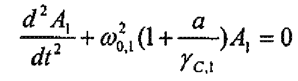

On peut poser α = α 0 + α v cos(2πfR t) a0 représentant la partie utile basse fréquence de l'accélération appliquée au capteur et αv étant une constante représentant l'amplitude des vibrations.We can put α = α 0 + α v cos (2πf R t ) a 0 representing the useful low frequency part of the acceleration applied to the sensor and α v being a constant representing the amplitude of the vibrations.
On pose I = A 1 et on note Q la transformée de Hilbert de I. Le spectre de I est celui d'un signal modulé en fréquence par un sinus. On a donc une raie principale centrée sur la fréquence 
En appliquant la transformée de Hilbert à la relation 2bis, on obtient alors : 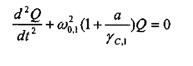
En posant I = ρcos(ϕ) et Q = ρsin(ϕ), avec p amplitude instantanée de I et ϕ phase instantanée de I, dans les deux équations différentielles précédentes, on obtient les deux équations suivantes 

On utilise, dans cette formulation et dans celles qui suivent, la notation simplifiée des dérivées qui consiste à indiquer l'ordre de dérivation par un exposant entre parenthèses. En multipliant la première relation par cos(ϕ) et la seconde par sin(ϕ), en effectuant une somme et en divisant par p , l'amplitude instantanée ne s'annulant pas, on obtient : 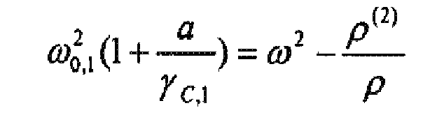
Dans le cas d'un accéléromètre à barreau vibrant, la tension de sortie U 1 de l'amplificateur de charge est proportionnelle au signal I. Le spectre du signal de position de l'oscillateur ne comprend alors pas de terme basse fréquence. En notant ω 1 la pulsation instantanée de U 1 et ρ 1 son amplitude instantanée, on 
On obtient ainsi 
A partir de la fonction 
En notant V 1 la transformée de Hilbert de U 1 et en utilisant la troisième propriété de la transformée de Hilbert on a alors : 
La fonction 
grâce à la fonction 
thanks to the
La réalisation pratique de cette fonction 
Sur cette figure, chaque rectangle représente un élément électronique assurant une fonction particulière. Ainsi, la transformée de Hilbert V1 est obtenue grâce à un filtre à réponse impulsionnelle finie noté FIRTH à N+1 points dont la bande spectrale inclut les raies d'amplitude significative du signal U1. Les dérivées des signaux sont calculées par un filtre à réponse impulsionnelle finie noté FIRD à L+1 points dont la bande spectrale inclut également ces raies. Afin d'assurer la synchronisation des signaux, le signal U1 doit être retardé de ![]()
![]()
![]()
![]()
![]()
![]()
On réalise ainsi une démodulation large bande du signal. La relation 
Il est à noter qu'en remplaçant I par ρcos(ϕ) et Q par ρsin(ϕ) dans leurs équations différentielles respectives, on obtient 2ρ'ω+ρω' = 0 soit ωρ 2 = constante. Toute variation de pulsation instantanée provoquée par une variation de l'accélération appliquée au capteur entraîne une variation d'amplitude instantanée. On démontre ainsi que le signal du capteur n'est pas modulé seulement en fréquence mais aussi en amplitude. Cette modulation d'amplitude n'est pas prise en compte dans les méthodes de l'art antérieur, ce qui engendre donc une erreur supplémentaire.It should be noted that by replacing I by ρ cos ( φ ) and Q by ρ sin ( φ ) in their respective differential equations, we obtain 2 ρ ' ω + ρω ' = 0 that is ωρ 2 = constant. Any variation in instantaneous pulsation caused by a variation of the acceleration applied to the sensor causes a variation instantaneous amplitude. It is thus demonstrated that the sensor signal is not modulated only in frequency but also in amplitude. This amplitude modulation is not taken into account in the methods of the prior art, which therefore generates an additional error.
On considère maintenant l'équation différentielle complète vérifiée par le résonateur : 
Le terme d'excitation e 1 s'écrit e 1 = K 4,1 (V 0 + v)2 + K 5,1 V 0 2
Avec V 0 : tension continue de polarisation et
ν : tension variable obtenue à partir d'un asservissement en phase et en amplitude sur la tension de sortie de l'amplificateur de charge représentant le signal de sortie du capteur. La tension ν se situe donc à la fréquence du résonateur.The term excitation e 1 is written e 1 = K 4.1 ( V 0 + v ) 2 + K 5.1 V 0 2
With V 0 : DC bias voltage and
ν: variable voltage obtained from a phase and amplitude feedback on the output voltage of the charge amplifier representing the output signal of the sensor. The voltage ν is therefore at the frequency of the resonator.
On suppose que l'asservissement en phase et en amplitude se fait parfaitement. On peut éliminer le terme d'amortissement. On a en effet: 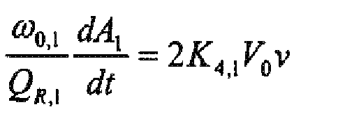
Le terme ν2 possède une composante à deux fois la fréquence de résonance qui n'intervient pas significativement dans l'équation et un terme continu négligeable par rapport au carré de la tension continue de polarisation.The term ν 2 has a component at twice the resonance frequency that does not significantly affect the equation and a negligible continuous term with respect to the square of the DC bias voltage.
L'équation devient ainsi : 
On cherche à décomposer la solution du mouvement sous la forme ![]()
Avec I signal haute fréquence dont le spectre est centré sur 
![]()
With I high frequency signal whose spectrum is centered on
Δ terme basse fréquence.Δ low frequency term.
On raisonne dans un premier temps en l'absence de non linéarité d'ordre 3. On pose alors 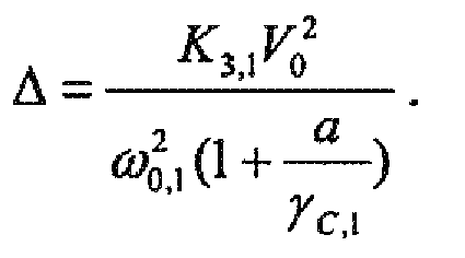
On considère la solution I de l'équation 

En l'absence de non linéarité d'ordre 3, on décompose donc la solution de l'équation (8) en un terme haute fréquence et un terme basse fréquence Δ défini par 
On néglige l'effet de la non linéarité sur ce terme basse fréquence. En effet, d'après les ordres de grandeur mis en jeu, on a 
On écrit donc A 1 = I + Δ avec I terme haute fréquence et Δ terme basse fréquence défini par 
L'équation 8 s'écrit : 
Equation 8 is written:
En appliquant la transformée de Hilbert à la relation 8 bis avec les mêmes notations que précédemment, on obtient, en notant H(αΔ) la transformée de Hilbert de αΔ, la relation 9 ci-dessous : 
En multipliant la relation 8 bis par I et la relation 9 par Q , on obtient : 
Dans le membre de droite de l'équation, les termes H(aΔ) et aΔ sont inconnus. On ne les prend pas en compte dans l'algorithme dans la mesure où ils provoquent une erreur négligeable.In the right-hand side of the equation, the terms H ( a Δ) and a Δ are unknown. They are not taken into account in the algorithm insofar as they cause a negligible error.
Les termes en ΔI, Δ 3 I et ![]()

![]()
Compte-tenu de ces simplifications, on obtient alors la relation suivante : 
a est l'accélération estimée par l'algorithme. Elle comprend l'accélération utile basse fréquence et les termes de vibration.Given these simplifications, we obtain the following relation:
a is the acceleration estimated by the algorithm. It includes useful low frequency acceleration and vibration terms.
On estime Δ par la relation 
La tension de sortie U 1 de l'amplificateur de charge est proportionnelle au signal I.U 1 = K1I . L'information Δ ayant un spectre basse fréquence n'est pas présente en sortie de l'amplificateur de charge. On obtient ainsi la relation 10 
On peut réécrire la relation, en utilisant la troisième propriété de la transformée de Hilbert, en notant ω 1 la pulsation instantanée de U 1 et ρ 1 l'amplitude instantanée de U 1. On obtient alors la relation 11 
L'accélération estimée s'obtient à partir de cette information par la relation 12 
On peut ainsi estimer l'accélération grâce à la fonction 
Cette fonction peut être calculée par la réalisation de la fonction 
L'accélération estimée par cet algorithme ne contient pas de biais significatif introduit par les vibrations. L'information renvoyée par l'algorithme varie linéairement en fonction de l'accélération appliquée au capteur.The acceleration estimated by this algorithm does not contain any significant bias introduced by the vibrations. The information returned by the algorithm varies linearly as a function of the acceleration applied to the sensor.
Par rapport à l'algorithme précédent, on voit apparaître deux termes supplémentaires :


Généralement, on emploie deux résonateurs ayant des axes sensibles de même direction et de sens opposé, sur deux voies différentes. On a, dans ce cas, sur chacune des voies des relations similaires liant Ω aux autres paramètres. Sur la voie 1, on a la relation 12 précédente et sur la voie 2 la relation 13 ci-dessous, en notant ω 2 pulsation instantanée deU 2 et ρ 2 amplitude instantanée de U 2 , U2 étant la tension en sortie du filtre sur la deuxième voie 
En utilisant la troisième propriété de la transformée de Hilbert, on montre que le terme de droite de la relation précédente peut être réalisé en utilisant U 2, sa transformée de Hilbert notée V 2 et leurs dérivées. On obtient alors la relation suivante : 
On peut montrer de la même manière que l'accélération peut être estimée sur cette voie grâce à la relation : 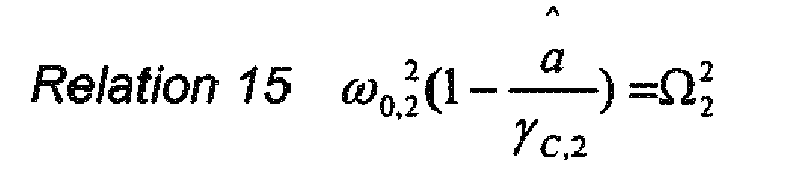
Partant de ces deux relations, il est possible d'effectuer un traitement différentiel, c'est à dire un traitement qui utilise les informations des deux voies du capteur et qui détermine à partir des informations renvoyées par chaque voie non seulement l'information d'accélération mais encore les dérives des principaux paramètres dues notamment à la température.Starting from these two relations, it is possible to perform a differential processing, ie a processing that uses the information of the two channels of the sensor and which determines from the information returned by each channel not only the information of acceleration but also the drifts of the main parameters due in particular to the temperature.
On peut utiliser la simple différence des deux informations, l'accélération pouvant être estimée grâce à la relation 
Cependant, si les termes en (ω 0 et en γC dérivent et sont fonction d'un paramètre comme la température, alors une mauvaise estimation de ladite température provoque alors :
- une erreur de biais par mauvaise estimation du
terme 
- une erreur de facteur d'échelle par mauvaise estimation du terme

- an error of bias by bad estimation of the
term - a scale factor error by mispricing the term
On peut notablement s'affranchir de ces difficultés en utilisant un traitement différentiel mieux adapté. On a vu que l'accélération était reliée aux informations renvoyées sur les deux voies par les relations 11 et 13. On estime les deux quantités suivantes :
- différence pondérée des deux
informations 
- somme pondérée des deux
informations 


- weighted difference of the two pieces of
information - weighted sum of both
information
L'accélération estimée de la relation 16 comprend alors la partie utile et les termes de vibration.The estimated acceleration of the relation 16 then comprises the useful part and the vibration terms.
En supposant que l'accélération critique et que la fréquence au repos varient suivant une loi exponentielle en fonction de la température, les rapports 
![]()
![]()
![]()
![]()
On peut réécrire ces deux relations en exprimant les paramètres physiques comme des polynômes fonction de la température. On suppose que la somme pondérée dépend de la température et également de l'accélération. On obtient ainsi 

Les coefficients αi et δi sont connus par calibration. Des informations ![]()
![]()
![]()
![]()
La réalisation pratique ne pose pas de problèmes particuliers. A titre d'exemple, le traitement différentiel est représenté sur la figure 4. On filtre la somme et la différence pondérée par un filtre coupe bande noté F.C.B. centré sur la fréquence des vibrations et par un filtre passe bas noté F.P.B. L'accélération estimée grâce à ces relations en sortie des filtres est alors uniquement l'accélération utile.The practical realization does not pose particular problems. By way of example, the differential treatment is represented in FIG. 4. The sum and the weighted difference are filtered by a cross-sectional filter denoted F.C.B. centered on the frequency of the vibrations and by a low pass filter noted F.P.B. The estimated acceleration due to these relationships at the output of the filters is then only the useful acceleration.
Claims (7)


représentative du carré de la pulsation de résonance Ω du dispositif vibrant, βi , K 1 et K 3 étant des constantes.Analysis system according to claim 3, characterized in that , when the vibrating device is forced oscillation, that is to say that the device comprises a phase and amplitude control arranged to eliminate the natural damping of the device, said servocontrol generating a polarization V 0 , said device then comprises third means making it possible to carry out, using the preceding notations, a third function equal to
representative of the square of the resonance pulse Ω of the vibrating device, β i , K 1 and K 3 being constants.


Applications Claiming Priority (1)
| Application Number | Priority Date | Filing Date | Title |
|---|---|---|---|
| FR0703733A FR2916533B1 (en) | 2007-05-25 | 2007-05-25 | SYSTEM FOR FREQUENCY ANALYSIS OF RESONANT DEVICES. |
Publications (3)
| Publication Number | Publication Date |
|---|---|
| EP1995575A2 true EP1995575A2 (en) | 2008-11-26 |
| EP1995575A3 EP1995575A3 (en) | 2018-01-17 |
| EP1995575B1 EP1995575B1 (en) | 2022-01-12 |
Family
ID=39227031
Family Applications (1)
| Application Number | Title | Priority Date | Filing Date |
|---|---|---|---|
| EP08156845.3A Active EP1995575B1 (en) | 2007-05-25 | 2008-05-23 | System for analysing the frequency of resonant devices |
Country Status (3)
| Country | Link |
|---|---|
| US (1) | US8220331B2 (en) |
| EP (1) | EP1995575B1 (en) |
| FR (1) | FR2916533B1 (en) |
Cited By (2)
| Publication number | Priority date | Publication date | Assignee | Title |
|---|---|---|---|---|
| EP2544011A1 (en) | 2011-07-08 | 2013-01-09 | Thales | Vibrating micro-system with automatic gain-control loop, with built-in monitoring of the quality factor |
| WO2013189700A1 (en) | 2012-06-22 | 2013-12-27 | Thales | Sensor with a vibrating member in a cavity, with integrated anomaly detection |
Families Citing this family (2)
| Publication number | Priority date | Publication date | Assignee | Title |
|---|---|---|---|---|
| KR102054962B1 (en) * | 2018-04-18 | 2019-12-12 | 경희대학교 산학협력단 | Wire sensing apparatus |
| CN112629647B (en) * | 2020-11-24 | 2022-04-08 | 同济大学 | Real-time identification, monitoring and early warning method for vortex vibration event of large-span suspension bridge |
Family Cites Families (8)
| Publication number | Priority date | Publication date | Assignee | Title |
|---|---|---|---|---|
| US2822515A (en) * | 1955-07-13 | 1958-02-04 | James M Klaasse | Spinning type magnetometer |
| US4761743A (en) | 1985-12-02 | 1988-08-02 | The Singer Company | Dynamic system analysis in a vibrating beam accelerometer |
| US5550516A (en) * | 1994-12-16 | 1996-08-27 | Honeywell Inc. | Integrated resonant microbeam sensor and transistor oscillator |
| US20040123665A1 (en) * | 2001-04-11 | 2004-07-01 | Blodgett David W. | Nondestructive detection of reinforcing member degradation |
| WO2002087083A1 (en) * | 2001-04-18 | 2002-10-31 | The Charles Stark Draper Laboratory, Inc. | Digital method and system for determining the instantaneous phase and amplitude of a vibratory accelerometer and other sensors |
| CN1309168C (en) * | 2001-06-18 | 2007-04-04 | 株式会社山武 | High frequency oscillation type proimity sensor |
| JP2004361388A (en) * | 2003-05-15 | 2004-12-24 | Mitsubishi Electric Corp | Capacitive type inertial force detection device |
| JP2005181394A (en) * | 2003-12-16 | 2005-07-07 | Canon Inc | Torsional vibrator, light deflector, and image forming apparatus |
-
2007
- 2007-05-25 FR FR0703733A patent/FR2916533B1/en not_active Expired - Fee Related
-
2008
- 2008-05-23 EP EP08156845.3A patent/EP1995575B1/en active Active
- 2008-05-23 US US12/126,820 patent/US8220331B2/en active Active
Cited By (3)
| Publication number | Priority date | Publication date | Assignee | Title |
|---|---|---|---|---|
| EP2544011A1 (en) | 2011-07-08 | 2013-01-09 | Thales | Vibrating micro-system with automatic gain-control loop, with built-in monitoring of the quality factor |
| WO2013189700A1 (en) | 2012-06-22 | 2013-12-27 | Thales | Sensor with a vibrating member in a cavity, with integrated anomaly detection |
| FR2992418A1 (en) * | 2012-06-22 | 2013-12-27 | Thales Sa | VIBRANT ELEMENT SENSOR IN A CAVITY WITH INTEGRAL DETECTION OF ANOMALIES |
Also Published As
| Publication number | Publication date |
|---|---|
| US20080289419A1 (en) | 2008-11-27 |
| FR2916533B1 (en) | 2012-12-28 |
| EP1995575B1 (en) | 2022-01-12 |
| US8220331B2 (en) | 2012-07-17 |
| FR2916533A1 (en) | 2008-11-28 |
| EP1995575A3 (en) | 2018-01-17 |
Similar Documents
| Publication | Publication Date | Title |
|---|---|---|
| EP0455530B1 (en) | Fibre optical measuring device, gyroscope, navigation and stabilisation system, current sensor | |
| EP2544011B1 (en) | Vibrating micro-system with automatic gain-control loop, with built-in monitoring of the quality factor | |
| EP3472558B1 (en) | Measuring system and gyrometer comprising such a system | |
| FR2729754A1 (en) | DEVICE AND METHOD FOR INCREASING THE RESOLUTION OF ANGULAR SPEED INFORMATION DETECTED FROM A RING LASER GYROSCOPE | |
| EP1730608A1 (en) | Method for modulating an atomic clock signal with coherent population trapping and corresponding atomic clock | |
| EP2936056B1 (en) | Gyroscope with simplified calibration and simplified calibration method for a gyroscope | |
| EP0161956B1 (en) | Method for the unambiguous doppler speed measurement of a moving object | |
| EP1995575B1 (en) | System for analysing the frequency of resonant devices | |
| EP2620751A1 (en) | Measurement device with resonant sensors | |
| EP3523644B1 (en) | Gas detector and method for measuring a gas concentration using photoacoustic effect | |
| EP0751373B1 (en) | Apparatus for measuring angular speed | |
| FR2827040A1 (en) | OFFSET REMOVAL SYSTEM FOR A VIBRATING GYROSCOPE | |
| EP0750176B1 (en) | Apparatus for measuring an angular speed | |
| EP3462188B1 (en) | Method for determining the quality factor of an oscillator | |
| EP0019511B1 (en) | Process for compensating temperature variations in surface-wave devices and pressure sensor for carrying out this process | |
| EP3462198B1 (en) | Method for determining characteristic parameters of an oscillator | |
| EP0750177B1 (en) | Apparatus and method for measuring angular speed | |
| FR2800869A1 (en) | Hemispherical resonator gyroscope (HRG) or other vibrating sensor has analysis electronics that enable the second harmonic to be eliminated allowing more precise measurements to be made | |
| EP3044697B1 (en) | Electronic method for extracting the amplitude and the phase of a signal in synchronous detection and interferometric assembly for implementing the method | |
| FR2729755A1 (en) | Ring laser gyroscope with phase error correction | |
| CN112424562B (en) | Path fluctuation monitoring for frequency modulated interferometers | |
| EP3469386B1 (en) | System and method for providing the amplitude and phase delay of a sinusoidal signal | |
| EP0371256B1 (en) | Apparatus for measuring a physical quantity | |
| EP4075156A1 (en) | Method for using a magnetometer with zero field optical pumping operated in a non-zero ambient field | |
| FR2892505A1 (en) | Directional system receives and processes intermediate frequency signals to output directional signals having same frequency |
Legal Events
| Date | Code | Title | Description |
|---|---|---|---|
| PUAI | Public reference made under article 153(3) epc to a published international application that has entered the european phase |
Free format text: ORIGINAL CODE: 0009012 |
|
| AK | Designated contracting states |
Kind code of ref document: A2 Designated state(s): AT BE BG CH CY CZ DE DK EE ES FI FR GB GR HR HU IE IS IT LI LT LU LV MC MT NL NO PL PT RO SE SI SK TR |
|
| AX | Request for extension of the european patent |
Extension state: AL BA MK RS |
|
| PUAL | Search report despatched |
Free format text: ORIGINAL CODE: 0009013 |
|
| AK | Designated contracting states |
Kind code of ref document: A3 Designated state(s): AT BE BG CH CY CZ DE DK EE ES FI FR GB GR HR HU IE IS IT LI LT LU LV MC MT NL NO PL PT RO SE SI SK TR |
|
| AX | Request for extension of the european patent |
Extension state: AL BA MK RS |
|
| RIC1 | Information provided on ipc code assigned before grant |
Ipc: G01P 15/097 20060101ALI20171213BHEP Ipc: G01H 13/00 20060101AFI20171213BHEP |
|
| STAA | Information on the status of an ep patent application or granted ep patent |
Free format text: STATUS: REQUEST FOR EXAMINATION WAS MADE |
|
| 17P | Request for examination filed |
Effective date: 20180711 |
|
| RBV | Designated contracting states (corrected) |
Designated state(s): AT BE BG CH CY CZ DE DK EE ES FI FR GB GR HR HU IE IS IT LI LT LU LV MC MT NL NO PL PT RO SE SI SK TR |
|
| AKX | Designation fees paid |
Designated state(s): AT BE BG CH CY CZ DE DK EE ES FI FR GB GR HR HU IE IS IT LI LT LU LV MC MT NL NO PL PT RO SE SI SK TR |
|
| AXX | Extension fees paid |
Extension state: MK Extension state: BA Extension state: RS Extension state: AL |
|
| GRAP | Despatch of communication of intention to grant a patent |
Free format text: ORIGINAL CODE: EPIDOSNIGR1 |
|
| STAA | Information on the status of an ep patent application or granted ep patent |
Free format text: STATUS: GRANT OF PATENT IS INTENDED |
|
| INTG | Intention to grant announced |
Effective date: 20210210 |
|
| GRAJ | Information related to disapproval of communication of intention to grant by the applicant or resumption of examination proceedings by the epo deleted |
Free format text: ORIGINAL CODE: EPIDOSDIGR1 |
|
| STAA | Information on the status of an ep patent application or granted ep patent |
Free format text: STATUS: REQUEST FOR EXAMINATION WAS MADE |
|
| RAP3 | Party data changed (applicant data changed or rights of an application transferred) |
Owner name: THALES |
|
| INTC | Intention to grant announced (deleted) | ||
| GRAP | Despatch of communication of intention to grant a patent |
Free format text: ORIGINAL CODE: EPIDOSNIGR1 |
|
| STAA | Information on the status of an ep patent application or granted ep patent |
Free format text: STATUS: GRANT OF PATENT IS INTENDED |
|
| INTG | Intention to grant announced |
Effective date: 20210614 |
|
| GRAS | Grant fee paid |
Free format text: ORIGINAL CODE: EPIDOSNIGR3 |
|
| GRAA | (expected) grant |
Free format text: ORIGINAL CODE: 0009210 |
|
| STAA | Information on the status of an ep patent application or granted ep patent |
Free format text: STATUS: THE PATENT HAS BEEN GRANTED |
|
| AK | Designated contracting states |
Kind code of ref document: B1 Designated state(s): AT BE BG CH CY CZ DE DK EE ES FI FR GB GR HR HU IE IS IT LI LT LU LV MC MT NL NO PL PT RO SE SI SK TR |
|
| REG | Reference to a national code |
Ref country code: GB Ref legal event code: FG4D Free format text: NOT ENGLISH |
|
| REG | Reference to a national code |
Ref country code: CH Ref legal event code: EP |
|
| REG | Reference to a national code |
Ref country code: DE Ref legal event code: R096 Ref document number: 602008064366 Country of ref document: DE |
|
| REG | Reference to a national code |
Ref country code: IE Ref legal event code: FG4D Free format text: LANGUAGE OF EP DOCUMENT: FRENCH |
|
| REG | Reference to a national code |
Ref country code: AT Ref legal event code: REF Ref document number: 1462686 Country of ref document: AT Kind code of ref document: T Effective date: 20220215 |
|
| REG | Reference to a national code |
Ref country code: LT Ref legal event code: MG9D |
|
| REG | Reference to a national code |
Ref country code: NL Ref legal event code: MP Effective date: 20220112 |
|
| REG | Reference to a national code |
Ref country code: AT Ref legal event code: MK05 Ref document number: 1462686 Country of ref document: AT Kind code of ref document: T Effective date: 20220112 |
|
| PG25 | Lapsed in a contracting state [announced via postgrant information from national office to epo] |
Ref country code: NL Free format text: LAPSE BECAUSE OF FAILURE TO SUBMIT A TRANSLATION OF THE DESCRIPTION OR TO PAY THE FEE WITHIN THE PRESCRIBED TIME-LIMIT Effective date: 20220112 |
|
| PG25 | Lapsed in a contracting state [announced via postgrant information from national office to epo] |
Ref country code: SE Free format text: LAPSE BECAUSE OF FAILURE TO SUBMIT A TRANSLATION OF THE DESCRIPTION OR TO PAY THE FEE WITHIN THE PRESCRIBED TIME-LIMIT Effective date: 20220112 Ref country code: PT Free format text: LAPSE BECAUSE OF FAILURE TO SUBMIT A TRANSLATION OF THE DESCRIPTION OR TO PAY THE FEE WITHIN THE PRESCRIBED TIME-LIMIT Effective date: 20220512 Ref country code: NO Free format text: LAPSE BECAUSE OF FAILURE TO SUBMIT A TRANSLATION OF THE DESCRIPTION OR TO PAY THE FEE WITHIN THE PRESCRIBED TIME-LIMIT Effective date: 20220412 Ref country code: LT Free format text: LAPSE BECAUSE OF FAILURE TO SUBMIT A TRANSLATION OF THE DESCRIPTION OR TO PAY THE FEE WITHIN THE PRESCRIBED TIME-LIMIT Effective date: 20220112 Ref country code: HR Free format text: LAPSE BECAUSE OF FAILURE TO SUBMIT A TRANSLATION OF THE DESCRIPTION OR TO PAY THE FEE WITHIN THE PRESCRIBED TIME-LIMIT Effective date: 20220112 Ref country code: ES Free format text: LAPSE BECAUSE OF FAILURE TO SUBMIT A TRANSLATION OF THE DESCRIPTION OR TO PAY THE FEE WITHIN THE PRESCRIBED TIME-LIMIT Effective date: 20220112 Ref country code: BG Free format text: LAPSE BECAUSE OF FAILURE TO SUBMIT A TRANSLATION OF THE DESCRIPTION OR TO PAY THE FEE WITHIN THE PRESCRIBED TIME-LIMIT Effective date: 20220412 |
|
| PG25 | Lapsed in a contracting state [announced via postgrant information from national office to epo] |
Ref country code: PL Free format text: LAPSE BECAUSE OF FAILURE TO SUBMIT A TRANSLATION OF THE DESCRIPTION OR TO PAY THE FEE WITHIN THE PRESCRIBED TIME-LIMIT Effective date: 20220112 Ref country code: LV Free format text: LAPSE BECAUSE OF FAILURE TO SUBMIT A TRANSLATION OF THE DESCRIPTION OR TO PAY THE FEE WITHIN THE PRESCRIBED TIME-LIMIT Effective date: 20220112 Ref country code: GR Free format text: LAPSE BECAUSE OF FAILURE TO SUBMIT A TRANSLATION OF THE DESCRIPTION OR TO PAY THE FEE WITHIN THE PRESCRIBED TIME-LIMIT Effective date: 20220413 Ref country code: FI Free format text: LAPSE BECAUSE OF FAILURE TO SUBMIT A TRANSLATION OF THE DESCRIPTION OR TO PAY THE FEE WITHIN THE PRESCRIBED TIME-LIMIT Effective date: 20220112 Ref country code: AT Free format text: LAPSE BECAUSE OF FAILURE TO SUBMIT A TRANSLATION OF THE DESCRIPTION OR TO PAY THE FEE WITHIN THE PRESCRIBED TIME-LIMIT Effective date: 20220112 |
|
| PG25 | Lapsed in a contracting state [announced via postgrant information from national office to epo] |
Ref country code: IS Free format text: LAPSE BECAUSE OF FAILURE TO SUBMIT A TRANSLATION OF THE DESCRIPTION OR TO PAY THE FEE WITHIN THE PRESCRIBED TIME-LIMIT Effective date: 20220512 |
|
| REG | Reference to a national code |
Ref country code: DE Ref legal event code: R097 Ref document number: 602008064366 Country of ref document: DE |
|
| PG25 | Lapsed in a contracting state [announced via postgrant information from national office to epo] |
Ref country code: SK Free format text: LAPSE BECAUSE OF FAILURE TO SUBMIT A TRANSLATION OF THE DESCRIPTION OR TO PAY THE FEE WITHIN THE PRESCRIBED TIME-LIMIT Effective date: 20220112 Ref country code: RO Free format text: LAPSE BECAUSE OF FAILURE TO SUBMIT A TRANSLATION OF THE DESCRIPTION OR TO PAY THE FEE WITHIN THE PRESCRIBED TIME-LIMIT Effective date: 20220112 Ref country code: EE Free format text: LAPSE BECAUSE OF FAILURE TO SUBMIT A TRANSLATION OF THE DESCRIPTION OR TO PAY THE FEE WITHIN THE PRESCRIBED TIME-LIMIT Effective date: 20220112 Ref country code: DK Free format text: LAPSE BECAUSE OF FAILURE TO SUBMIT A TRANSLATION OF THE DESCRIPTION OR TO PAY THE FEE WITHIN THE PRESCRIBED TIME-LIMIT Effective date: 20220112 Ref country code: CZ Free format text: LAPSE BECAUSE OF FAILURE TO SUBMIT A TRANSLATION OF THE DESCRIPTION OR TO PAY THE FEE WITHIN THE PRESCRIBED TIME-LIMIT Effective date: 20220112 |
|
| PLBE | No opposition filed within time limit |
Free format text: ORIGINAL CODE: 0009261 |
|
| STAA | Information on the status of an ep patent application or granted ep patent |
Free format text: STATUS: NO OPPOSITION FILED WITHIN TIME LIMIT |
|
| 26N | No opposition filed |
Effective date: 20221013 |
|
| REG | Reference to a national code |
Ref country code: BE Ref legal event code: MM Effective date: 20220531 |
|
| GBPC | Gb: european patent ceased through non-payment of renewal fee |
Effective date: 20220523 |
|
| PG25 | Lapsed in a contracting state [announced via postgrant information from national office to epo] |
Ref country code: MC Free format text: LAPSE BECAUSE OF FAILURE TO SUBMIT A TRANSLATION OF THE DESCRIPTION OR TO PAY THE FEE WITHIN THE PRESCRIBED TIME-LIMIT Effective date: 20220112 Ref country code: LU Free format text: LAPSE BECAUSE OF NON-PAYMENT OF DUE FEES Effective date: 20220523 |
|
| PG25 | Lapsed in a contracting state [announced via postgrant information from national office to epo] |
Ref country code: SI Free format text: LAPSE BECAUSE OF FAILURE TO SUBMIT A TRANSLATION OF THE DESCRIPTION OR TO PAY THE FEE WITHIN THE PRESCRIBED TIME-LIMIT Effective date: 20220112 |
|
| PG25 | Lapsed in a contracting state [announced via postgrant information from national office to epo] |
Ref country code: IE Free format text: LAPSE BECAUSE OF NON-PAYMENT OF DUE FEES Effective date: 20220523 |
|
| PG25 | Lapsed in a contracting state [announced via postgrant information from national office to epo] |
Ref country code: GB Free format text: LAPSE BECAUSE OF NON-PAYMENT OF DUE FEES Effective date: 20220523 Ref country code: BE Free format text: LAPSE BECAUSE OF NON-PAYMENT OF DUE FEES Effective date: 20220531 |
|
| P01 | Opt-out of the competence of the unified patent court (upc) registered |
Effective date: 20230427 |
|
| PG25 | Lapsed in a contracting state [announced via postgrant information from national office to epo] |
Ref country code: IT Free format text: LAPSE BECAUSE OF FAILURE TO SUBMIT A TRANSLATION OF THE DESCRIPTION OR TO PAY THE FEE WITHIN THE PRESCRIBED TIME-LIMIT Effective date: 20220112 |
|
| PGFP | Annual fee paid to national office [announced via postgrant information from national office to epo] |
Ref country code: FR Payment date: 20230421 Year of fee payment: 16 Ref country code: DE Payment date: 20230418 Year of fee payment: 16 Ref country code: CH Payment date: 20230602 Year of fee payment: 16 |
|
| PG25 | Lapsed in a contracting state [announced via postgrant information from national office to epo] |
Ref country code: HU Free format text: LAPSE BECAUSE OF FAILURE TO SUBMIT A TRANSLATION OF THE DESCRIPTION OR TO PAY THE FEE WITHIN THE PRESCRIBED TIME-LIMIT; INVALID AB INITIO Effective date: 20080523 |