EP1865340B1 - A process and program for characterising evolution of an oil reservoir over time - Google Patents
A process and program for characterising evolution of an oil reservoir over time Download PDFInfo
- Publication number
- EP1865340B1 EP1865340B1 EP06290912A EP06290912A EP1865340B1 EP 1865340 B1 EP1865340 B1 EP 1865340B1 EP 06290912 A EP06290912 A EP 06290912A EP 06290912 A EP06290912 A EP 06290912A EP 1865340 B1 EP1865340 B1 EP 1865340B1
- Authority
- EP
- European Patent Office
- Prior art keywords
- time
- survey
- velocity
- seismic
- reservoir
- Prior art date
- Legal status (The legal status is an assumption and is not a legal conclusion. Google has not performed a legal analysis and makes no representation as to the accuracy of the status listed.)
- Active
Links
Images


Classifications
-
- G—PHYSICS
- G01—MEASURING; TESTING
- G01V—GEOPHYSICS; GRAVITATIONAL MEASUREMENTS; DETECTING MASSES OR OBJECTS; TAGS
- G01V1/00—Seismology; Seismic or acoustic prospecting or detecting
- G01V1/28—Processing seismic data, e.g. analysis, for interpretation, for correction
- G01V1/30—Analysis
-
- G—PHYSICS
- G01—MEASURING; TESTING
- G01V—GEOPHYSICS; GRAVITATIONAL MEASUREMENTS; DETECTING MASSES OR OBJECTS; TAGS
- G01V1/00—Seismology; Seismic or acoustic prospecting or detecting
- G01V1/28—Processing seismic data, e.g. analysis, for interpretation, for correction
- G01V1/30—Analysis
- G01V1/308—Time lapse or 4D effects, e.g. production related effects to the formation
-
- G—PHYSICS
- G01—MEASURING; TESTING
- G01V—GEOPHYSICS; GRAVITATIONAL MEASUREMENTS; DETECTING MASSES OR OBJECTS; TAGS
- G01V2210/00—Details of seismic processing or analysis
- G01V2210/60—Analysis
- G01V2210/61—Analysis by combining or comparing a seismic data set with other data
- G01V2210/612—Previously recorded data, e.g. time-lapse or 4D
-
- G—PHYSICS
- G01—MEASURING; TESTING
- G01V—GEOPHYSICS; GRAVITATIONAL MEASUREMENTS; DETECTING MASSES OR OBJECTS; TAGS
- G01V2210/00—Details of seismic processing or analysis
- G01V2210/60—Analysis
- G01V2210/61—Analysis by combining or comparing a seismic data set with other data
- G01V2210/614—Synthetically generated data
Definitions
- the present invention relates to the field of geophysics and more particularly to oil exploration.
- the imaging process aims to place the reflected waves at the position of the corresponding reflectors; the vertical coordinate may be given as depth or an equivalent vertical time depending upon the choice of processing strategy.
- the process normally requires a model of the velocity of propagation of seismic waves in the sub-surface.
- Standard imaging velocity packages such as the one sold by Paradigm (IL) under reference Geodepth make it possible to build such models of the seismic velocity field.
- 4D seismic involves comparing 3D seismic surveys carried out at different time instances.
- the aim is to observe changes in the state of the reservoir and surrounding formations consequent upon production of hydrocarbons from that reservoir. This generally requires greater care in acquisition than for standard 3D surveys followed by specialised processing steps.
- Document WO-A-2005/066660 discloses a method of processing seismic data representing a physical system, the method comprising: forming a difference between first and second seismic data representing the system in first and second states, respectively; and inverting the difference in accordance with a parameterised model of the physical system to obtain changes in the parameters of the model.
- the invention therefore provides a process for characterising the evolution of a oil reservoir in the process of producing by co-analyzing the changes in the propagation times and seismic amplitudes of seismic reflections, comprising the steps of
- the invention provides a computer program residing on a computer-readable medium, comprising computer program code means adapted to run on a computer all the steps of such a process.
- base survey and "monitor survey” for designating the seismic surveys of the reservoir.
- the assumption is that the base survey is carried out earlier in time than the monitor survey.
- the invention is based on the fact that changes in the reservoir, due to exploitation, will cause changes to the velocity field. Practically, oil will be substituted by gas or water and the fluid pressure will change, causing changes in density and moduli, and thus changes in velocity. Changes within the reservoir may also change the stress and strain state of the surrounding rocks, further causing changes in their velocities. These changes to velocity will produce time shifts in the seismic expression of underlying reflectors and associated changes in reflectivity, causing a change in the local waveform.
- the invention suggests, in one embodiment, to assess these effects in the monitor survey. This makes it possible to deduce from the comparison of the base and monitor survey a field of velocity changes, without having to proceed with cross correlation of the traces.
- Figure 1 is a schematic view of a seismic block, showing one trace only for the sake of clarity.
- seismic block is used for describing a set of measurements, over a given geographical field, after processing to produce an image.
- the term seismic block is used for describing a set of measurements, over a given geographical field, after processing to produce an image.
- one uses an orthogonal and normalized set of coordinates, in which the x and y axes lie in the horizontal plane.
- the z-axis which corresponds to time, is vertical and oriented downward.
- one uses the coordinates (x, y, t) for a temporal representation of the survey, or the coordinates (x, y, z) after depth migration to a spatial representation of the survey.
- the sensors may be hydrophones in streamers which are typically towed at 5-7m depth; alternatively receiver cables may be placed on the ocean bottom; even land geophones may sometimes be buried a few metres deep.
- a raw signal is recorded on each sensor C i ; this raw signal is representative of the seismic waves reflected by the various interfaces in the sub-surface.
- Raw signals received on sensors are then processed to provide an image of the sub-surface comprised of a collection of vertical seismic traces, the vertical axis representing time t or depth z.
- Figure 1 shows the axes x, y and t (or z) of the set of coordinates, as well as one sensor C i with the corresponding trace, referenced 2 on the figure.
- figure 1 only shows one sensor and one trace, while a survey would typically involve many sensors and a number of traces higher than one million.
- seismic processing will place the seismic events as accurately as possible in their true lateral positions. In the idealised case of zero dip and zero offset, with no lateral velocity gradients, this would be directly beneath the sensors, but in general the positions will be effectively independent of the original positions of the sensors.
- FIG. 2 is a flowchart of a process according to one embodiment of the invention.
- step 12 there is provided a base survey of the reservoir, with a set of seismic traces at a first time T.
- the base survey provides an amplitude b(t), that is an amplitude which is a function of time t; with digital recording and processing the trace is sampled at a set of values t i , with i an index; typical trace lengths correspond to around 1000 samples at a 4 ms sampling period.
- the trace is then handled as a set of values b(t i ) or b i .
- one provides a monitor survey of the reservoir, taken at a second time T + ⁇ T, with a set of seismic traces.
- ⁇ T is a positive quantity
- the monitor survey is taken at a time later than the base survey; however, the order in which the surveys are taken is irrelevant to the operation of the process of the invention and, in principle, the time lapse ⁇ T could as well be negative - which amounts to comparing the earlier survey to the later one.
- a sampled trace in the monitor survey is represented as a set of values m(t i ) or m i .
- the traces in the monitor survey are associated to the same positions as in the base survey. This is carried out by using, inasmuch as possible, the same equipment, acquisition geometry and processes for running the base survey and monitor survey. Practically speaking, a difference of 5-10 m between the positions of sources and receivers still leads to acceptable results. Techniques such as interpolation may be used in case traces in the monitor survey and in the base survey do not fulfil this condition ( Eiken, O., et al., 2003, A proven method for acquiring highly repeatable towed streamer seismic data, Geophysics, 68, 1303-1309 ).
- V b and V m are notionally the local vertical velocities, considered for 3D warping. They do not in general match any velocities used in prior seismic processing, that is migration velocities or stacking velocities. Their difference is indicative of vertical time shifts of seismic events between base and monitor.
- This relative slowness change, n may be assessed in each sample of the seismic block, that is in each sample of a trace. For estimating the relative slowness change, one uses optimization over a set of points, as explained below.
- This expression is representative of the fact that the time shift w i for sample i on the trace is caused by velocity changes above the sample. Strictly speaking, the time shift is the integrated change of slowness over the path followed by the signal from the source to the sample being considered and back.
- the expression given above is based on the assumption that time shifts derive from velocity changes above the sample being considered; this corresponds to a vertical or quasi-vertical propagation path from source to reflector and back to the sensor.
- the second term is representative of the effect of the local change of reflectivity, consequent upon the velocity change, on the trace; in this second term, local change is considered in a time range commensurate to the wavelet, that is in a time range equal to the duration of the wavelet.
- This difference ⁇ i is the difference between the amplitude b i of the seismic trace in the base survey at the point i and the sum of
- This provides a field of velocity changes, for the various points.
- the field of velocity changes parameterises a warping operation for aligning the monitor survey with the base and may also be used for directly characterizing the evolution of the reservoir.
- step 16 of the process of figure 2 a set of points is selected; the sum S will be minimized on this set of points.
- the size of the set of points may vary, but these will normally be chosen to completely include the full volume of the reservoir under consideration.
- the traces from the entire base and monitor surveys, windowed in time to span the reservoir are used. This will provide values of velocity changes over the complete surveys.
- step 20 of the process the sum S is minimized, by varying the values of the relative velocity changes.
- An optimization technique is provided below; however, one may also use other optimization techniques known per se in the art, such as simulated annealing. If, as suggested above, the seismic events in the monitor survey are not displaced laterally from their positions in the base survey, points are only time-shifted. One may then carry out the computation on a trace-by-trace basis; in other words, optimization may be carried out separately on each trace. This simplifies computation and makes it easier to run the optimization step as parallel tasks on a number of computers.
- step 22 the minimum of sum S has been attained, and this provides a value of velocity change for the various points of the set of points over which the optimization was carried out.
- the field of velocity changes associated with the minimum of the sum S characterizes the evolution of the reservoir over time.
- the wavelet may be scaled accordingly. For example, if there is a positive correlation such that, on average, a 1% change in velocity implies a 0.25% change in density, the wavelet could be scaled by a factor 1.25 so as to give the most probable representation of the change in the trace resulting from the velocity perturbation.
- the process of figure 2 was applied to surveys of the Girassol field.
- the base survey was carried out in the year 1999 by CGG as a high-resolution survey, with sampling of 2ms. Production started in 2001, and the monitor survey was carried out in the year 2002, using the same equipment as the base survey.
- Each survey comprises 2.5 million traces, of around 2000 samples each, which were windowed to 500 samples for the application of the method described herein, in the embodiment detailed above.
- the process of figure 2 was carried out using the velocity field originally modelled for the base survey; the velocity field for processing the monitor survey was taken to be the same as that of the base, for the purpose of the time-lapse comparison. Since the base and monitor surveys were carried out under very similar conditions, and dips are small, optimization was carried out on a trace by trace basis. The process was carried out in 20 hours on 60 processors in parallel, that is around 1200 CPU hours; convergence was achieved in 3 iterations in the optimization process.
- the evaluation of the difference ⁇ i will take the amplitude value from the monitor seismic block which has been displaced not only by a time shift, but also by a change in lateral position.
- the overall displacements between the migrated images are due to velocity changes along the propagation paths, which are no longer vertical; for a given point i, the corresponding point i' is then shifted in time and in space along the propagation path defined by the migration process which created the images, by an amount which corresponds to the integral, along the true propagation path, of the slowness changes in the earth.
- Figures 3-7 show a 2D synthetic test of the process of figure 2 ; the test was carried out by applying velocity changes to actual data, computing the monitor survey based on the velocity changes, and then applying the process for reconstructing the velocity changes.
- Figure 3 shows a section through the seismic image block derived from the base survey. This section is derived from actual data from the Girassol field, obtained by convolutional modelling of the p-wave impedance cube derived by inversion of the base seismic data. As discussed in reference to figure 1 , the horizontal axis shows the trace numbers - or the distance along the section; the vertical axis represents time. Amplitude appears in figure 3 for each trace; one sees that the dip in the reservoir is substantially zero, with maximum values of dip around 3° and RMS values of dip in the reservoir around 1.5°.
- Figure 4 shows the velocity changes imposed in the synthetic test.
- the velocity change has a "butterfly", design, which gives easy appreciation of the inversion result and the potential resolution and stability of the method.
- velocity changes are positive, with a constant value of +8%; on the right side of the butterfly, velocity changes are negative, with a constant value of -8%.
- Figure 5 shows the changes of amplitude caused by the velocity changes of figure 4 . Specifically, figure 5 results from
- Figure 6 shows the results of the process of figure 2 . It shows the differences in amplitudes, after minimising sum S, between the base and the shifted monitor surveys, revealing the estimated changes in amplitudes due to the change of reflectivity only. In the example, optimization was carried out on a trace by trace basis, and converged in 3 iterations.
- Figure 6 shows that amplitude changes substantially reflect the velocity changes of figure 3 ; this shows the efficacy of the process. In particular the alignment of the traces below the velocity changes is sufficiently good that the difference traces are effectively zero in this region.
- Figure 7 shows the velocity changes, computed during the process of optimization. Although there are some errors, figure 7 shows that the values of velocity changes are substantially those of figure 3 .
- Spectral analysis of the velocity perturbation shows that the inversion has a broad-band nature, with frequencies recovered from 0Hz out to the upper limit of the seismic spectrum, and thus that the inverted velocity change attribute may be quantitative and easily interpretable.
- Figures 8 and 9 show a more realistic 2D synthetic test of the process of figure 2 ; the test was carried out by applying velocity changes to actual data, with more complex velocity changes. Specifically, velocity changes were placed in interpreted sand bodies, as shown in figure 8 .
- Figure 9 shows the results obtained in the process of the invention; changes in velocity again substantially correspond to those of figure 8 . As in the example of figures 3-7 , the spectra of the estimated changes confirm the broad-band nature of the calculation.
- Figures 8 and 9 show that the process will also operate on velocity changes more complex that the ones of figure 3 .
- Figures 10-13 show the results obtained thanks to the process of figure 2 , on the actual surveys for the Girassol field.
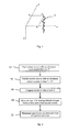
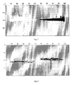
- Figure 10 is a section of the raw differences between the monitor survey and base survey, on Girassol fast-track near substacks; figure 10 is taken along crossline 4001 of the survey.
- Figure 11 shows the seismic amplitude difference computed in the process of figure 2 ; compared to figure 10 , one can see that the differences are now for the major part visible in the upper part of the section; this part corresponds to the portions of the reservoir wherefrom oil is being retrieved.
- figures 10-13 shows that the process of the invention provides results that are immediately usable and are also in accordance with exploration data.
- Spectral analysis of the data of figures 10-12 also shows, as in the previous examples, that lower frequencies are well recovered.
- figures 10-12 is carried out on the Girassol near substacks, where the average incidence angles amount to 12 degrees; therefore, even though the warp displacements may be vertical, they may not be exactly equal to the vertical integral of the superposed slowness changes; the example of figures 10-12 demonstrates that deviations from the assumption of zero-offset and dip which arise in real cases can be tolerated and the method yields results that appear realistic and quantitatively meaningful.
- the process of the invention may be embodied in a computer program.
- the program is adapted to receive data for the base and monitor surveys, as well as data for the velocity fields; such data are in the format provided by state of the art computer packages such as those discussed above.
- the program runs the various steps of the process of figure 2 .
Abstract
Description
- The present invention relates to the field of geophysics and more particularly to oil exploration.
- It is the aim of oil exploration to determine the position of oil-bearing reservoirs on the basis of the results of geophysical measurements made from the surface or in drilling wells. These measurements typically involve sending a seismic wave into the sub-surface and measuring with a number of sensors the various reflections of the wave off geological structures - surfaces separating distinct materials, faults, etc. (reflection seismic surveying). Other measurements are made from wells. Acoustic waves, gamma radiations or electrical signals are then sent into the sub-surface; again, a number of sensors are used for sensing the reflected signals. Such sensors may be disposed on the ground or at sea.
- These techniques typically involve the processing of the measurements so as to construct an image of the sub-surface. The imaging process aims to place the reflected waves at the position of the corresponding reflectors; the vertical coordinate may be given as depth or an equivalent vertical time depending upon the choice of processing strategy. The process normally requires a model of the velocity of propagation of seismic waves in the sub-surface. Standard imaging velocity packages, such as the one sold by Paradigm (IL) under reference Geodepth make it possible to build such models of the seismic velocity field.
- These techniques can be extended to allow observation of the evolution of a given reservoir over time - e.g. before oil production starts and after some period of oil production and to compare the results of measurements. This is called 4D seismic and involves comparing 3D seismic surveys carried out at different time instances. The aim is to observe changes in the state of the reservoir and surrounding formations consequent upon production of hydrocarbons from that reservoir. This generally requires greater care in acquisition than for standard 3D surveys followed by specialised processing steps.
- Document
WO-A-2005/066660 discloses a method of processing seismic data representing a physical system, the method comprising: forming a difference between first and second seismic data representing the system in first and second states, respectively; and inverting the difference in accordance with a parameterised model of the physical system to obtain changes in the parameters of the model. - J.E. Rickett & D.E. Lumley, Cross-equalization data processing for time-lapse seismic reservoir monitoring : A case study from the Gulf of Mexico, J. E. Rickett & D. E. Lumley, Cross-equalization data processing for time-lapse seismic reservoir monitoring : A case study from the Gulf of Mexico, Geophysics, vol. 66 no. 4 (July-August 2001), pp. 1015-1025 discusses the problem of non-repeatable noise in seismic surveys carried out over time. This document discloses the matching of two actual surveys. Pre-migration data were not available. Matching of surveys include matched filtering, amplitude balancing and 3D warping. 3D warping consists in cross-correlating traces within windows to assess movements in x, y and t adapted to optimise matching of data between surveys.
- Hall et al., Cross-matching with interpreted warping of 3D streamer and 3D ocean-bottom-cable data at Valhall for time-lapse assessment, Geophysical Prospecting, 2005, 53, pp. 283-297 discloses cross-matching of legacy streamer data and newer 3D ocean-bottom cable data, for time-lapse analysis of geomechanical changes due to production in the Valhall field. This document is directed to using results provided by different acquisition methodologies - in the example of the Valhall field, 3D streamer data and 3D ocean-bottom cable. The document indicates that similar migration schemes were used for both surveys. The process involves the steps of
- volumetric shaping, to take into account the different acquisition methodologies;
- amplitude balancing within and between volumes;
- spectral shaping;
- global cross-matching, using a locally derived operator.
- O. Kolbjornsen & A.R. Syversveen, Time-match- a method for estimating 4D time shift, Norks Regnesentral, note no. SAND/03/05, April 2005, discusses a method for estimating time shifts in 4D seismic survey. The algorithm used matches the times of imaged reflectors in a new survey with the times in the original survey; providing a map from one to the other, on a trace by trace basis. Specifically, matching is carried out by locally compressing and stretching the time axis of, e.g., traces from the monitor survey in order to minimize the squared difference between amplitudes. This note discusses a synthetic test case.
- These documents of the prior art teach 3D warping, the realignment of the seismic surveys being compared for compensating both faults in acquisition (or non-repeatability of seismic surveys) and changes in velocity in the sub-surface. One problem with correlation-based approaches is the size of the correlation window. If the window used for correlation is too large, the accuracy of correlation is likely to be affected: indeed, the correlation value will then depend not only on differences between the survey at the point being considered, but also on other effects, apart from the points being considered. If the window used for correlation is too small, correlation is likely to be severely affected by noise and non-repeatability of the surveys, including changes due to the effects whose observation is desired.
- There is still a need for a process for characterising the evolution of a reservoir in time, which could mitigate this problem.
- In an embodiment, the invention therefore provides a process for characterising the evolution of a oil reservoir in the process of producing by co-analyzing the changes in the propagation times and seismic amplitudes of seismic reflections, comprising the steps of
- providing a base survey of the reservoir with a set of seismic traces at a first time T associated to a first velocity Vb ;
- providing a monitor survey of the reservoir, taken at a second time T + ΔT, with a set of seismic traces associated to the same positions as in the base survey, associated to a second velocity Vm;
- for a set of points in the base survey, computing the sum S over the points of the set of a norm of the difference between
the amplitude bi of the seismic trace in the base survey at said point i and the sum of the amplitude mi, of the seismic trace at a time-corresponding point i' in the monitor survey and the amplitude due to the reflectivity change local to the said time-corresponding point i' induced by the relative change in the velocity of the earth in and around the reservoir (difference between the first velocity Vb and the second velocity Vm;) - characterising the evolution of the oil reservoir by minimizing the sum S.
- In one embodiment, the amplitude due to reflectivity change local to said time-corresponding point is computed over a time range of one to five times the length of a wavelet used in the surveys. A time range of the order of the length of the wavelet is preferable.
- One may also provide that a corresponding point i' is only shifted in time. In this instance, the step of optimizing may be carried out on a trace by trace basis.
- In another embodiment, a corresponding point i' is shifted in time and in space along the propagation path.
- The process may further comprise, as preprocessing, the step of zero-offsetting a survey.
- In another embodiment, the invention provides a computer program residing on a computer-readable medium, comprising computer program code means adapted to run on a computer all the steps of such a process.
- A process embodying the invention will now be described, by way of nonlimiting example, and in reference to the accompanying drawings, where :
-
figure 1 is a schematic view of a seismic block, showing one trace only for the sake of clarity; -
figure 2 is a flowchart of a process in one embodiment of the invention; -
figure 3 shows a section of a seismic block used for the base survey in a 2D synthetic test of the process offigure 2 ; -
figure 4 shows the velocity changes imposed in the synthetic test; -
figure 5 shows the changes of amplitude caused by the velocity changes offigure 4 ; -
figure 6 shows the results of the process offigure 2 ; -
figure 7 shows the velocity changes, computed during the process of optimization; -
figure 8 shows velocity changes places in interpreted sand bodies, for another 2D synthetic test; -
figure 9 shows the results obtained in the process offigure 2 ; -
figure 10 is a section of the raw differences between the monitor survey and base survey in an actual example; -
figure 11 shows the seismic amplitude difference computed according to the process offigure 2 ; -
figure 12 shows the impedance difference estimated by a leading contractor in the same region; -
figure 13 shows the proportional velocity changes in part of the section offigures 10 and11 ; - In the rest of this description, one will use the terms "base survey" and "monitor survey" for designating the seismic surveys of the reservoir. The assumption is that the base survey is carried out earlier in time than the monitor survey.
- The invention is based on the fact that changes in the reservoir, due to exploitation, will cause changes to the velocity field. Practically, oil will be substituted by gas or water and the fluid pressure will change, causing changes in density and moduli, and thus changes in velocity. Changes within the reservoir may also change the stress and strain state of the surrounding rocks, further causing changes in their velocities. These changes to velocity will produce time shifts in the seismic expression of underlying reflectors and associated changes in reflectivity, causing a change in the local waveform. The invention suggests, in one embodiment, to assess these effects in the monitor survey. This makes it possible to deduce from the comparison of the base and monitor survey a field of velocity changes, without having to proceed with cross correlation of the traces.
- This approach is particularly effective where the change in density is expected to be relatively small and the effective reflection angle is small (and/or the expected changes in the shear-wave velocity are also relatively small). For the sake of facilitating computation, it is further advantageous to assume that the time shifts come uniquely from velocity changes and that changes in acquisition or processing parameters are negligible. The latter assumption is increasingly fulfilled in modem, dedicated 4D surveys. The first of these conditions will be fulfilled when the pressure effect on the frame moduli is the dominant time-lapse phenomenon or when small amounts of gas are released or introduced into a previously 100% liquid pore fluid. As shown in the examples below, the method is particularly applicable for analysing time warping of the near offset substack.
-
Figure 1 is a schematic view of a seismic block, showing one trace only for the sake of clarity. The term seismic block is used for describing a set of measurements, over a given geographical field, after processing to produce an image. As known per se, one uses an orthogonal and normalized set of coordinates, in which the x and y axes lie in the horizontal plane. The z-axis, which corresponds to time, is vertical and oriented downward. As usual for seismic surveys, one uses the coordinates (x, y, t) for a temporal representation of the survey, or the coordinates (x, y, z) after depth migration to a spatial representation of the survey. A set of sensors Ci are placed on the ground or at sea, in points of spatial coordinates (xi, yi, zi), i being an integer representative of the sensor number; although much of the literature appears to subscribe to the fiction that zi=0, the sensors are rarely placed exactly at zi=0. In marine acquisition, the sensors may be hydrophones in streamers which are typically towed at 5-7m depth; alternatively receiver cables may be placed on the ocean bottom; even land geophones may sometimes be buried a few metres deep. When a survey is carried out, a raw signal is recorded on each sensor Ci; this raw signal is representative of the seismic waves reflected by the various interfaces in the sub-surface. Raw signals received on sensors are then processed to provide an image of the sub-surface comprised of a collection of vertical seismic traces, the vertical axis representing time t or depth z.Figure 1 shows the axes x, y and t (or z) of the set of coordinates, as well as one sensor Ci with the corresponding trace, referenced 2 on the figure. For the sake of clarity,figure 1 only shows one sensor and one trace, while a survey would typically involve many sensors and a number of traces higher than one million. As known per se, seismic processing will place the seismic events as accurately as possible in their true lateral positions. In the idealised case of zero dip and zero offset, with no lateral velocity gradients, this would be directly beneath the sensors, but in general the positions will be effectively independent of the original positions of the sensors. - Details on these techniques are available in Özdogan Yilmaz, Seismic Data Processing, Society of exploration Geophysicists, 1987.
-
Figure 2 is a flowchart of a process according to one embodiment of the invention. Instep 12, there is provided a base survey of the reservoir, with a set of seismic traces at a first time T. For a given trace, the base survey provides an amplitude b(t), that is an amplitude which is a function of time t; with digital recording and processing the trace is sampled at a set of values ti , with i an index; typical trace lengths correspond to around 1000 samples at a 4 ms sampling period. The trace is then handled as a set of values b(ti) or bi. - At
step 16, one provides a monitor survey of the reservoir, taken at a second time T + ΔT, with a set of seismic traces. In the simplest assumption, ΔT is a positive quantity, and the monitor survey is taken at a time later than the base survey; however, the order in which the surveys are taken is irrelevant to the operation of the process of the invention and, in principle, the time lapse ΔT could as well be negative - which amounts to comparing the earlier survey to the later one. As for the base survey, a sampled trace in the monitor survey is represented as a set of values m(ti) or mi. - Ideally, the traces in the monitor survey are associated to the same positions as in the base survey. This is carried out by using, inasmuch as possible, the same equipment, acquisition geometry and processes for running the base survey and monitor survey. Practically speaking, a difference of 5-10 m between the positions of sources and receivers still leads to acceptable results. Techniques such as interpolation may be used in case traces in the monitor survey and in the base survey do not fulfil this condition (Eiken, O., et al., 2003, A proven method for acquiring highly repeatable towed streamer seismic data, Geophysics, 68, 1303-1309).
- In this embodiment, the invention results in estimating the relative slowness change, n, where slowness is the reciprocal of velocity, with

In that formula, Vb and Vm are notionally the local vertical velocities, considered for 3D warping. They do not in general match any velocities used in prior seismic processing, that is migration velocities or stacking velocities. Their difference is indicative of vertical time shifts of seismic events between base and monitor. - This relative slowness change, n, may be assessed in each sample of the seismic block, that is in each sample of a trace. For estimating the relative slowness change, one uses optimization over a set of points, as explained below.
- On a given trace, time shift w; (in units of samples) can be expressed for a given sample i as follows

with nk the relative slowness change for sample k. This expression is representative of the fact that the time shift wi for sample i on the trace is caused by velocity changes above the sample. Strictly speaking, the time shift is the integrated change of slowness over the path followed by the signal from the source to the sample being considered and back. The expression given above is based on the assumption that time shifts derive from velocity changes above the sample being considered; this corresponds to a vertical or quasi-vertical propagation path from source to reflector and back to the sensor. This condition is fulfilled at zero offset, that is when the distance between the sender and the sensor which is zero or which may be neglected compared to the vertical depth of the reflectors, and when the value of dip is zero or is limited; the dip is the angle formed between the normals to a horizontal plane and local reflectors. Practically speaking, because we are usually concerned only with propagation through the region where production-related changes are occurring, in the reservoir, these assumptions need only apply over the reservoir thickness; furthermore, "zero" lateral displacement corresponds to remaining within a seismic bin. That is, for a reservoir of thickness around 100m, and a seismic bin size of 25m, these assumptions would allow for propagation paths with a lateral displacement of up to 12.5 m between the entry into the reservoir zone (on the way down from the source) and the reflection point, and a similar displacement on the way back up to the sensor, or to a dip of up to 14° for a zero-offset trace. These assumptions may be relaxed further in most cases, where some continuity is expected between bins, or where the 4D survey is used in the context of informing a reservoir model, where grid cells typically have horizontal dimensions of the order of 100m. - Under these assumptions, the change in velocity from the base survey to the monitor survey will impact the amplitude in a given trace so that

where ψ is the seismic wavelet and n(ti) = n(ti) - n(t i-1). (Note that we are implicitly expressing the times in sample units.) The first term is indicative of the time shift induced by velocity changes above sample i under the assumptions given above. The second term is representative of the effect of the local change of reflectivity, consequent upon the velocity change, on the trace; in this second term, local change is considered in a time range commensurate to the wavelet, that is in a time range equal to the duration of the wavelet. - The invention suggests assessing the change in velocity from the base survey to the monitor survey and thus characterising the evolution of the reservoir by assessing the sum, over various points of the base survey, of the norm of the difference

This difference Δ i is the difference between the amplitude bi of the seismic trace in the base survey at the point i and the sum of - the amplitude mi' of the seismic trace at a time-corresponding point i' in the monitor survey and
- that amplitude perturbation due to the reflectivity change local to the said time-corresponding point i' induced by the difference between the first velocity Vb and the second velocity Vm.
- The sum S of the norm of the difference over the various points

is minimized by varying the modelled velocity changes - expressed as the relative slowness changes ni . This provides a field of velocity changes, for the various points. The field of velocity changes parameterises a warping operation for aligning the monitor survey with the base and may also be used for directly characterizing the evolution of the reservoir. - In
step 16 of the process offigure 2 , a set of points is selected; the sum S will be minimized on this set of points. According to computational resources, one may vary the size of the set of points, but these will normally be chosen to completely include the full volume of the reservoir under consideration. In the examples provided below, the traces from the entire base and monitor surveys, windowed in time to span the reservoir, are used. This will provide values of velocity changes over the complete surveys. - In
step 18 of the process, an initial value of the sum S is computed. - In
step 20 of the process, the sum S is minimized, by varying the values of the relative velocity changes. One example of an optimization technique is provided below; however, one may also use other optimization techniques known per se in the art, such as simulated annealing. If, as suggested above, the seismic events in the monitor survey are not displaced laterally from their positions in the base survey, points are only time-shifted. One may then carry out the computation on a trace-by-trace basis; in other words, optimization may be carried out separately on each trace. This simplifies computation and makes it easier to run the optimization step as parallel tasks on a number of computers. - In
step 22, the minimum of sum S has been attained, and this provides a value of velocity change for the various points of the set of points over which the optimization was carried out. The field of velocity changes associated with the minimum of the sum S, characterizes the evolution of the reservoir over time. - Minimization in
step 20 may be carried out using the Gauss-Newton formula. The Gauss-Newton formula is known per se. - Tests carried out by the applicant suggest that convergence will generally be achieved after 2-4 iterations. It is ascertained that the process will converge if the time shifts amount to less than a half-period of the dominant frequency, as will often be the case. Beyond this value, there may be a risk that the Gauss-Newton iteration will converge on a local minimum. The fact that the above embodiment of the process may converge on a local minimum does not invalidate the method, inasmuch as a correct selection of the initial values of the relative slowness changes, using, e.g., a standard correlation method, such that the remaining shifts are less than a half-period, or interpreting and matching major seismic markers in and around the reservoir, will allow its subsequent application. Alternatively, the use of a global optimisation approach will ensure convergence toward the true minimum.
- In the case where density changes are thought to be non-negligible, but statistically correlated with the velocity changes, the wavelet may be scaled accordingly. For example, if there is a positive correlation such that, on average, a 1% change in velocity implies a 0.25% change in density, the wavelet could be scaled by a factor 1.25 so as to give the most probable representation of the change in the trace resulting from the velocity perturbation.
- The process of
figure 2 was applied to surveys of the Girassol field. The base survey was carried out in the year 1999 by CGG as a high-resolution survey, with sampling of 2ms. Production started in 2001, and the monitor survey was carried out in the year 2002, using the same equipment as the base survey. Each survey comprises 2.5 million traces, of around 2000 samples each, which were windowed to 500 samples for the application of the method described herein, in the embodiment detailed above. The process offigure 2 was carried out using the velocity field originally modelled for the base survey; the velocity field for processing the monitor survey was taken to be the same as that of the base, for the purpose of the time-lapse comparison. Since the base and monitor surveys were carried out under very similar conditions, and dips are small, optimization was carried out on a trace by trace basis. The process was carried out in 20 hours on 60 processors in parallel, that is around 1200 CPU hours; convergence was achieved in 3 iterations in the optimization process. - In the example of
figure 2 , the events represented in the traces in the monitor survey are assumed to be in the same lateral positions as in the base survey. Thus we may consider that changes in the traces are only caused by time shifts, due to the changes in velocity along them (in the zero-offset, zero-dip, assumption) and associated changes in reflectivity. However, the process of the invention also applies where dips are not negligible, so that observed changes in the traces are caused not only by time shift, but also by lateral shifts of the seismic reflections. In other words, the process of the invention may still be carried out if the lateral positions of the events represented in the traces are perturbed in the monitor survey relative to those in the base survey. In this case, the evaluation of the difference Δ i will take the amplitude value from the monitor seismic block which has been displaced not only by a time shift, but also by a change in lateral position. The overall displacements between the migrated images are due to velocity changes along the propagation paths, which are no longer vertical; for a given point i, the corresponding point i' is then shifted in time and in space along the propagation path defined by the migration process which created the images, by an amount which corresponds to the integral, along the true propagation path, of the slowness changes in the earth. There will also be an amplitude change at i', as before, due to the change in local reflectivity associated with the velocity changes in the neighbourhood of that point. This will require some additional effort, compared to the embodiment previously described, to define these propagation paths and compute the relevant integrals. A similar process may then apply to the non-zero-offset case; even in the case where dips are small, and thus the displacements are mainly vertical, the time shifts are associated with slowness integrals along propagation paths that are largely outside the seismic bin containing the amplitude samples being compared. -
Figures 3-7 show a 2D synthetic test of the process offigure 2 ; the test was carried out by applying velocity changes to actual data, computing the monitor survey based on the velocity changes, and then applying the process for reconstructing the velocity changes. -
Figure 3 shows a section through the seismic image block derived from the base survey. This section is derived from actual data from the Girassol field, obtained by convolutional modelling of the p-wave impedance cube derived by inversion of the base seismic data. As discussed in reference tofigure 1 , the horizontal axis shows the trace numbers - or the distance along the section; the vertical axis represents time. Amplitude appears infigure 3 for each trace; one sees that the dip in the reservoir is substantially zero, with maximum values of dip around 3° and RMS values of dip in the reservoir around 1.5°. -
Figure 4 shows the velocity changes imposed in the synthetic test. The velocity change has a "butterfly", design, which gives easy appreciation of the inversion result and the potential resolution and stability of the method. On the left side of the butterfly, velocity changes are positive, with a constant value of +8%; on the right side of the butterfly, velocity changes are negative, with a constant value of -8%. -
Figure 5 shows the changes of amplitude caused by the velocity changes offigure 4 . Specifically,figure 5 results from - the computation of changes of amplitude caused in the data of
figure 3 , due to the velocity changes offigure 4 ; the changes are computed using propagation tools, with a velocity field equal to the sum of the base velocity field and of the butterfly changes offigure 4 ; - the computation of the difference between the computed amplitudes and the amplitudes of
figure 3 . -
Figure 6 shows the results of the process offigure 2 . It shows the differences in amplitudes, after minimising sum S, between the base and the shifted monitor surveys, revealing the estimated changes in amplitudes due to the change of reflectivity only. In the example, optimization was carried out on a trace by trace basis, and converged in 3 iterations.Figure 6 shows that amplitude changes substantially reflect the velocity changes offigure 3 ; this shows the efficacy of the process. In particular the alignment of the traces below the velocity changes is sufficiently good that the difference traces are effectively zero in this region. -
Figure 7 shows the velocity changes, computed during the process of optimization. Although there are some errors,figure 7 shows that the values of velocity changes are substantially those offigure 3 . Spectral analysis of the velocity perturbation shows that the inversion has a broad-band nature, with frequencies recovered from 0Hz out to the upper limit of the seismic spectrum, and thus that the inverted velocity change attribute may be quantitative and easily interpretable. -
Figures 8 and9 show a more realistic 2D synthetic test of the process offigure 2 ; the test was carried out by applying velocity changes to actual data, with more complex velocity changes. Specifically, velocity changes were placed in interpreted sand bodies, as shown infigure 8 .Figure 9 shows the results obtained in the process of the invention; changes in velocity again substantially correspond to those offigure 8 . As in the example offigures 3-7 , the spectra of the estimated changes confirm the broad-band nature of the calculation.Figures 8 and9 show that the process will also operate on velocity changes more complex that the ones offigure 3 . -
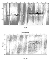
Figures 10-13 show the results obtained thanks to the process offigure 2 , on the actual surveys for the Girassol field.Figure 10 is a section of the raw differences between the monitor survey and base survey, on Girassol fast-track near substacks;figure 10 is taken along crossline 4001 of the survey.Figure 11 shows the seismic amplitude difference computed in the process offigure 2 ; compared tofigure 10 , one can see that the differences are now for the major part visible in the upper part of the section; this part corresponds to the portions of the reservoir wherefrom oil is being retrieved. In the lower part of the reservoir, differences in amplitude are much lower in the section offigure 11 than in the section offigure 10 ; this is caused by the fact that the process offigure 2 takes into account time shifts created in the upper lever.Figure 13 shows the proportional velocity changes in part of the section offigures 10 and11 near a well, as estimated in the optimization process offigure 2 ; this may be compared withfigure 12 , which shows the impedance difference estimated by a leading contractor in the same region. The improvement in interpretability arising from the broad-band nature of the velocity-change attribute is clear, and our confidence in the quantitative values of the attribute is accordingly enhanced.Figure 13 , by the absence of noise, also demonstrates the stability with which the velocity change attribute may be calculated by this approach, which we believe to be considerably improved in comparison with calculations based on the other approaches cited above. - The example of
figures 10-13 shows that the process of the invention provides results that are immediately usable and are also in accordance with exploration data. Spectral analysis of the data offigures 10-12 also shows, as in the previous examples, that lower frequencies are well recovered. - The example of
figures 10-12 is carried out on the Girassol near substacks, where the average incidence angles amount to 12 degrees; therefore, even though the warp displacements may be vertical, they may not be exactly equal to the vertical integral of the superposed slowness changes; the example offigures 10-12 demonstrates that deviations from the assumption of zero-offset and dip which arise in real cases can be tolerated and the method yields results that appear realistic and quantitatively meaningful. - The process of the invention may be embodied in a computer program. The program is adapted to receive data for the base and monitor surveys, as well as data for the velocity fields; such data are in the format provided by state of the art computer packages such as those discussed above. The program runs the various steps of the process of
figure 2 .
Claims (7)
- A process for characterising the evolution of a hydrocarbon reservoir in the process of producing by co-analyzing the changes in the propagation times and seismic amplitudes of a seismic wavelet along propagation paths in the ground, comprising the steps of- providing (12) a base survey of the reservoir with a set of seismic traces at a first time T associated to a first velocity Vb ;- providing (16) a monitor survey of the reservoir, taken at a second time T + ΔT, with a set of seismic traces associated to the same positions as in the base survey, associated to a second velocity Vm ;- for a set of points in the base survey, computing (18) the sum S over the points of the set of a norm of the difference between
the amplitude bi of the seismic trace in the base survey at said point i and the sum of the amplitude mi of the seismic trace at a time-corresponding point i' in the monitor survey and the amplitude due to the reflectivity change local to the said time-corresponding point i' induced by the relative change in the velocity of the earth in and around the reservoir which is the difference between the first velocity Vb and the second velocity Vm ;
wherein the time-corresponding point i' is shifted in time by a time-shift derived from the velocity changes along the propagation path from the surface to said time-corresponding point i';- characterising (22) the evolution of the reservoir by minimizing the sum S. - The process of claim 1, wherein the amplitude due to reflectivity change local to said time-corresponding point is computed over a time range of one to five times the length of a wavelet used in the surveys.
- The process of claim 1 or 2, wherein a corresponding point i' is only shifted in time.
- The process of claim 3, wherein the step of optimizing is carried out on a trace by trace basis.
- The process of claim 1 or 2, wherein a corresponding point i' is shifted in time and in space along the propagation path.
- The process of one of claims 1 to 5, further comprising before the step of computing, the step of zero-offsetting a survey.
- A computer program residing on a computer-readable medium, comprising computer program code means adapted to run on a computer all the steps of the process according to one of claims 1 to 6.
Priority Applications (6)
| Application Number | Priority Date | Filing Date | Title |
|---|---|---|---|
| AT06290912T ATE483175T1 (en) | 2006-06-06 | 2006-06-06 | METHOD AND PROGRAM FOR CHARACTERIZING THE TEMPORARY DEVELOPMENT OF A PETROLEUM REQUIREMENT |
| DE602006017186T DE602006017186D1 (en) | 2006-06-06 | 2006-06-06 | Method and program for characterizing the temporal evolution of a petroleum resource |
| EP06290912A EP1865340B1 (en) | 2006-06-06 | 2006-06-06 | A process and program for characterising evolution of an oil reservoir over time |
| US11/751,883 US7577061B2 (en) | 2006-06-06 | 2007-05-22 | Process and program for characterising evolution of an oil reservoir over time |
| CN2007101104629A CN101086535B (en) | 2006-06-06 | 2007-06-05 | A process and program for characterising evolution of an oil reservoir over time |
| NO20072844A NO338866B1 (en) | 2006-06-06 | 2007-06-05 | Process and computer program for characterizing the development of an oil reservoir over time |
Applications Claiming Priority (1)
| Application Number | Priority Date | Filing Date | Title |
|---|---|---|---|
| EP06290912A EP1865340B1 (en) | 2006-06-06 | 2006-06-06 | A process and program for characterising evolution of an oil reservoir over time |
Publications (2)
| Publication Number | Publication Date |
|---|---|
| EP1865340A1 EP1865340A1 (en) | 2007-12-12 |
| EP1865340B1 true EP1865340B1 (en) | 2010-09-29 |
Family
ID=37199201
Family Applications (1)
| Application Number | Title | Priority Date | Filing Date |
|---|---|---|---|
| EP06290912A Active EP1865340B1 (en) | 2006-06-06 | 2006-06-06 | A process and program for characterising evolution of an oil reservoir over time |
Country Status (6)
| Country | Link |
|---|---|
| US (1) | US7577061B2 (en) |
| EP (1) | EP1865340B1 (en) |
| CN (1) | CN101086535B (en) |
| AT (1) | ATE483175T1 (en) |
| DE (1) | DE602006017186D1 (en) |
| NO (1) | NO338866B1 (en) |
Families Citing this family (45)
| Publication number | Priority date | Publication date | Assignee | Title |
|---|---|---|---|---|
| EP2153246B1 (en) * | 2007-05-09 | 2015-09-16 | ExxonMobil Upstream Research Company | Inversion of 4d seismic data |
| FR2918066B1 (en) | 2007-06-26 | 2010-11-19 | Total France | NON-GELIFIABLE CONCENTRATE BINDER AND POMPABLE FOR BITUMEN / POLYMER |
| US8768672B2 (en) * | 2007-08-24 | 2014-07-01 | ExxonMobil. Upstream Research Company | Method for predicting time-lapse seismic timeshifts by computer simulation |
| US8548782B2 (en) * | 2007-08-24 | 2013-10-01 | Exxonmobil Upstream Research Company | Method for modeling deformation in subsurface strata |
| GB2469979B (en) * | 2008-03-07 | 2012-04-04 | Shell Int Research | Method of marine time-lapse seismic surveying |
| FR2929616B1 (en) * | 2008-04-08 | 2011-09-09 | Total France | PROCESS FOR CROSSLINKING BITUMEN / POLYMER COMPOSITIONS HAVING REDUCED EMISSIONS OF HYDROGEN SULFIDE |
| WO2009145960A1 (en) | 2008-04-17 | 2009-12-03 | Exxonmobil Upstream Research Company | Robust optimization-based decision support tool for reservoir development planning |
| EP2291761A4 (en) | 2008-04-18 | 2013-01-16 | Exxonmobil Upstream Res Co | Markov decision process-based decision support tool for reservoir development planning |
| WO2009131761A2 (en) | 2008-04-21 | 2009-10-29 | Exxonmobile Upstream Research Company | Stochastic programming-based decision support tool for reservoir development planning |
| FR2933499B1 (en) | 2008-07-03 | 2010-08-20 | Inst Francais Du Petrole | METHOD OF JOINT INVERSION OF SEISMIC DATA REPRESENTED ON DIFFERENT TIME SCALES |
| US8724429B2 (en) | 2008-12-17 | 2014-05-13 | Exxonmobil Upstream Research Company | System and method for performing time-lapse monitor surverying using sparse monitor data |
| US8705317B2 (en) | 2008-12-17 | 2014-04-22 | Exxonmobil Upstream Research Company | Method for imaging of targeted reflectors |
| AU2009333603B2 (en) | 2008-12-17 | 2014-07-24 | Exxonmobil Upstream Research Company | System and method for reconstruction of time-lapse data |
| US8451683B2 (en) * | 2009-04-03 | 2013-05-28 | Exxonmobil Upstream Research Company | Method for determining the fluid/pressure distribution of hydrocarbon reservoirs from 4D seismic data |
| US8332154B2 (en) | 2009-06-02 | 2012-12-11 | Exxonmobil Upstream Research Company | Estimating reservoir properties from 4D seismic data |
| US9110190B2 (en) * | 2009-06-03 | 2015-08-18 | Geoscale, Inc. | Methods and systems for multicomponent time-lapse seismic measurement to calculate time strains and a system for verifying and calibrating a geomechanical reservoir simulator response |
| GB2470760B (en) | 2009-06-04 | 2013-07-24 | Total Sa | An improved process for characterising the evolution of an oil or gas reservoir over time |
| CN101625420B (en) * | 2009-07-22 | 2012-05-09 | 中国石化集团胜利石油管理局 | Reservoir description method |
| CA2776487C (en) | 2009-11-12 | 2017-02-14 | Exxonmobil Upstream Research Company | Method and apparatus for generating a three-dimentional simulation grid for a reservoir model |
| GB2479347B (en) * | 2010-04-06 | 2015-10-21 | Total Sa | A process of characterising the evolution of an oil reservoir |
| GB2481444B (en) | 2010-06-25 | 2016-08-17 | Total Sa | An improved process for characterising the evolution of an oil or gas reservoir over time |
| FR2963111B1 (en) | 2010-07-21 | 2012-09-28 | Total Sa | METHOD FOR ESTIMATING ELASTIC PARAMETERS BY INVERTING SEISMIC 4D MEASUREMENTS |
| US8040754B1 (en) | 2010-08-27 | 2011-10-18 | Board Of Regents Of The University Of Texas System | System and method for acquisition and processing of elastic wavefield seismic data |
| US8243548B2 (en) | 2010-08-27 | 2012-08-14 | Board Of Regents Of The University Of Texas System | Extracting SV shear data from P-wave seismic data |
| US8325559B2 (en) | 2010-08-27 | 2012-12-04 | Board Of Regents Of The University Of Texas System | Extracting SV shear data from P-wave marine data |
| FR2965066B1 (en) | 2010-09-20 | 2012-10-26 | Total Sa | METHOD FOR ESTIMATING ELASTIC PARAMETERS |
| GB2489677A (en) * | 2011-03-29 | 2012-10-10 | Total Sa | Characterising the evolution of a reservoir over time from seismic surveys, making allowance for actual propagation paths through non-horizontal layers |
| WO2013009944A1 (en) * | 2011-07-12 | 2013-01-17 | Colorado School Of Mines | Wave-equation migration velocity analysis using image warping |
| US20150205002A1 (en) * | 2012-07-25 | 2015-07-23 | Schlumberger Technology Corporation | Methods for Interpretation of Time-Lapse Borehole Seismic Data for Reservoir Monitoring |
| WO2014177633A2 (en) * | 2013-05-01 | 2014-11-06 | Cgg Services Sa | Device and method for optimization of 4d and 3d seismic data |
| US10353096B2 (en) | 2013-12-16 | 2019-07-16 | Cgg Services Sas | Time-lapse simultaneous inversion of amplitudes and time shifts constrained by pre-computed input maps |
| CN103643949B (en) * | 2013-12-20 | 2016-06-01 | 中国石油天然气集团公司 | A kind of reservoir contains quantitative forecast method and the device of oil gas |
| GB2523109B (en) | 2014-02-12 | 2020-07-29 | Total E&P Uk Ltd | A process for characterising the evolution of an oil or gas reservoir over time |
| FR3019908B1 (en) | 2014-04-14 | 2016-05-06 | Total Sa | METHOD OF PROCESSING SEISMIC IMAGES |
| GB2528129A (en) | 2014-07-11 | 2016-01-13 | Total E&P Uk Ltd | Method for obtaining estimates of a model parameter so as to characterise the evolution of a subsurface volume |
| GB2528130A (en) | 2014-07-11 | 2016-01-13 | Total E&P Uk Ltd | Method of constraining an inversion in the characterisation of the evolution of a subsurface volume |
| WO2016046633A1 (en) * | 2014-09-22 | 2016-03-31 | Cgg Services Sa | Simultaneous multi-vintage time-lapse full waveform inversion |
| US10379244B2 (en) | 2015-01-06 | 2019-08-13 | Total S.A. | Method for obtaining estimates of a model parameter so as to characterise the evolution of a subsurface volume over a time period |
| CN109804273B (en) * | 2016-10-06 | 2022-01-11 | 国际壳牌研究有限公司 | Method for borehole time shift monitoring using seismic waves |
| EP3669210B1 (en) | 2017-08-17 | 2021-04-07 | Total Se | Method for obtaining estimates of a model parameter so as to characterise the evolution of a subsurface volume over a time period using time-lapse seismic |
| US11933929B2 (en) * | 2018-02-06 | 2024-03-19 | Conocophillips Company | 4D seismic as a method for characterizing fracture network and fluid distribution in unconventional reservoir |
| CN110888162B (en) * | 2018-09-07 | 2021-09-17 | 中国石油化工股份有限公司 | Method and system for enhancing continuity of same phase axis based on thermodynamic statistics |
| CN111856559B (en) * | 2019-04-30 | 2023-02-28 | 中国石油天然气股份有限公司 | Multi-channel seismic spectrum inversion method and system based on sparse Bayes learning theory |
| BR112021021740A2 (en) * | 2019-05-02 | 2022-01-04 | Bp Corp North America Inc | Joint inversion of displacement in time and 4d amplitude for velocity perturbation |
| US11372123B2 (en) | 2019-10-07 | 2022-06-28 | Exxonmobil Upstream Research Company | Method for determining convergence in full wavefield inversion of 4D seismic data |
Family Cites Families (5)
| Publication number | Priority date | Publication date | Assignee | Title |
|---|---|---|---|---|
| US6041018A (en) * | 1997-11-13 | 2000-03-21 | Colorado School Of Mines | Method for correcting amplitude and phase differences between time-lapse seismic surveys |
| CN1186648C (en) * | 2001-09-30 | 2005-01-26 | 中海油田服务股份有限公司 | Oil deposit testing ground surface data acquisition and treatment system and its data acquisition treatment method and equipment |
| WO2005040858A1 (en) * | 2003-10-24 | 2005-05-06 | Shell Internationale Research Maatschappij B.V. | Time-lapse seismic survey of a reservoir region |
| GB2409900B (en) | 2004-01-09 | 2006-05-24 | Statoil Asa | Processing seismic data representing a physical system |
| US7626887B2 (en) * | 2006-04-19 | 2009-12-01 | Westerngeco L.L.C. | Displacement field calculation |
-
2006
- 2006-06-06 EP EP06290912A patent/EP1865340B1/en active Active
- 2006-06-06 AT AT06290912T patent/ATE483175T1/en not_active IP Right Cessation
- 2006-06-06 DE DE602006017186T patent/DE602006017186D1/en active Active
-
2007
- 2007-05-22 US US11/751,883 patent/US7577061B2/en active Active
- 2007-06-05 CN CN2007101104629A patent/CN101086535B/en not_active Expired - Fee Related
- 2007-06-05 NO NO20072844A patent/NO338866B1/en unknown
Also Published As
| Publication number | Publication date |
|---|---|
| CN101086535A (en) | 2007-12-12 |
| ATE483175T1 (en) | 2010-10-15 |
| EP1865340A1 (en) | 2007-12-12 |
| US7577061B2 (en) | 2009-08-18 |
| DE602006017186D1 (en) | 2010-11-11 |
| NO20072844L (en) | 2007-12-07 |
| NO338866B1 (en) | 2016-10-31 |
| US20080291781A1 (en) | 2008-11-27 |
| CN101086535B (en) | 2011-12-07 |
Similar Documents
| Publication | Publication Date | Title |
|---|---|---|
| EP1865340B1 (en) | A process and program for characterising evolution of an oil reservoir over time | |
| US11428834B2 (en) | Processes and systems for generating a high-resolution velocity model of a subterranean formation using iterative full-waveform inversion | |
| AU2013200475B2 (en) | Methods and systems for correction of streamer-depth bias in marine seismic surveys | |
| US8352190B2 (en) | Method for analyzing multiple geophysical data sets | |
| CA2775561C (en) | Migration-based illumination determination for ava risk assessment | |
| US8209125B2 (en) | Method for identifying and analyzing faults/fractures using reflected and diffracted waves | |
| US20130289879A1 (en) | Process for characterising the evolution of a reservoir | |
| CA2940406C (en) | Characterizing a physical structure using a multidimensional noise model to attenuate noise data | |
| EP3359982B1 (en) | Seismic sensor orientation | |
| AU4133396A (en) | Method of seismic signal processing and exploration | |
| US11609349B2 (en) | Determining properties of a subterranean formation using an acoustic wave equation with a reflectivity parameterization | |
| EP2745146A1 (en) | System and method for subsurface characterization including uncertainty estimation | |
| US20220373703A1 (en) | Methods and systems for generating an image of a subterranean formation based on low frequency reconstructed seismic data | |
| Woo et al. | Improvement of fault interpretation with seismic attribute analysis of Jeju Basin, offshore southern Korea, East China Sea | |
| Redshaw | 2D and 3D seismic data |
Legal Events
| Date | Code | Title | Description |
|---|---|---|---|
| PUAI | Public reference made under article 153(3) epc to a published international application that has entered the european phase |
Free format text: ORIGINAL CODE: 0009012 |
|
| AK | Designated contracting states |
Kind code of ref document: A1 Designated state(s): AT BE BG CH CY CZ DE DK EE ES FI FR GB GR HU IE IS IT LI LT LU LV MC NL PL PT RO SE SI SK TR |
|
| AX | Request for extension of the european patent |
Extension state: AL BA HR MK YU |
|
| 17P | Request for examination filed |
Effective date: 20080612 |
|
| 17Q | First examination report despatched |
Effective date: 20080715 |
|
| AKX | Designation fees paid |
Designated state(s): AT BE BG CH CY CZ DE DK EE ES FI FR GB GR HU IE IS IT LI LT LU LV MC NL PL PT RO SE SI SK TR |
|
| GRAP | Despatch of communication of intention to grant a patent |
Free format text: ORIGINAL CODE: EPIDOSNIGR1 |
|
| GRAS | Grant fee paid |
Free format text: ORIGINAL CODE: EPIDOSNIGR3 |
|
| GRAJ | Information related to disapproval of communication of intention to grant by the applicant or resumption of examination proceedings by the epo deleted |
Free format text: ORIGINAL CODE: EPIDOSDIGR1 |
|
| GRAL | Information related to payment of fee for publishing/printing deleted |
Free format text: ORIGINAL CODE: EPIDOSDIGR3 |
|
| GRAP | Despatch of communication of intention to grant a patent |
Free format text: ORIGINAL CODE: EPIDOSNIGR1 |
|
| GRAS | Grant fee paid |
Free format text: ORIGINAL CODE: EPIDOSNIGR3 |
|
| GRAA | (expected) grant |
Free format text: ORIGINAL CODE: 0009210 |
|
| AK | Designated contracting states |
Kind code of ref document: B1 Designated state(s): AT BE BG CH CY CZ DE DK EE ES FI FR GB GR HU IE IS IT LI LT LU LV MC NL PL PT RO SE SI SK TR |
|
| REG | Reference to a national code |
Ref country code: GB Ref legal event code: FG4D |
|
| REG | Reference to a national code |
Ref country code: CH Ref legal event code: EP |
|
| REG | Reference to a national code |
Ref country code: IE Ref legal event code: FG4D |
|
| REF | Corresponds to: |
Ref document number: 602006017186 Country of ref document: DE Date of ref document: 20101111 Kind code of ref document: P |
|
| PG25 | Lapsed in a contracting state [announced via postgrant information from national office to epo] |
Ref country code: FI Free format text: LAPSE BECAUSE OF FAILURE TO SUBMIT A TRANSLATION OF THE DESCRIPTION OR TO PAY THE FEE WITHIN THE PRESCRIBED TIME-LIMIT Effective date: 20100929 Ref country code: LT Free format text: LAPSE BECAUSE OF FAILURE TO SUBMIT A TRANSLATION OF THE DESCRIPTION OR TO PAY THE FEE WITHIN THE PRESCRIBED TIME-LIMIT Effective date: 20100929 Ref country code: AT Free format text: LAPSE BECAUSE OF FAILURE TO SUBMIT A TRANSLATION OF THE DESCRIPTION OR TO PAY THE FEE WITHIN THE PRESCRIBED TIME-LIMIT Effective date: 20100929 |
|
| REG | Reference to a national code |
Ref country code: NL Ref legal event code: VDEP Effective date: 20100929 |
|
| LTIE | Lt: invalidation of european patent or patent extension |
Effective date: 20100929 |
|
| PG25 | Lapsed in a contracting state [announced via postgrant information from national office to epo] |
Ref country code: SI Free format text: LAPSE BECAUSE OF FAILURE TO SUBMIT A TRANSLATION OF THE DESCRIPTION OR TO PAY THE FEE WITHIN THE PRESCRIBED TIME-LIMIT Effective date: 20100929 |
|
| PG25 | Lapsed in a contracting state [announced via postgrant information from national office to epo] |
Ref country code: LV Free format text: LAPSE BECAUSE OF FAILURE TO SUBMIT A TRANSLATION OF THE DESCRIPTION OR TO PAY THE FEE WITHIN THE PRESCRIBED TIME-LIMIT Effective date: 20100929 Ref country code: GR Free format text: LAPSE BECAUSE OF FAILURE TO SUBMIT A TRANSLATION OF THE DESCRIPTION OR TO PAY THE FEE WITHIN THE PRESCRIBED TIME-LIMIT Effective date: 20101230 Ref country code: SE Free format text: LAPSE BECAUSE OF FAILURE TO SUBMIT A TRANSLATION OF THE DESCRIPTION OR TO PAY THE FEE WITHIN THE PRESCRIBED TIME-LIMIT Effective date: 20100929 |
|
| PG25 | Lapsed in a contracting state [announced via postgrant information from national office to epo] |
Ref country code: SK Free format text: LAPSE BECAUSE OF FAILURE TO SUBMIT A TRANSLATION OF THE DESCRIPTION OR TO PAY THE FEE WITHIN THE PRESCRIBED TIME-LIMIT Effective date: 20100929 Ref country code: NL Free format text: LAPSE BECAUSE OF FAILURE TO SUBMIT A TRANSLATION OF THE DESCRIPTION OR TO PAY THE FEE WITHIN THE PRESCRIBED TIME-LIMIT Effective date: 20100929 Ref country code: IS Free format text: LAPSE BECAUSE OF FAILURE TO SUBMIT A TRANSLATION OF THE DESCRIPTION OR TO PAY THE FEE WITHIN THE PRESCRIBED TIME-LIMIT Effective date: 20110129 Ref country code: IT Free format text: LAPSE BECAUSE OF FAILURE TO SUBMIT A TRANSLATION OF THE DESCRIPTION OR TO PAY THE FEE WITHIN THE PRESCRIBED TIME-LIMIT Effective date: 20100929 Ref country code: CZ Free format text: LAPSE BECAUSE OF FAILURE TO SUBMIT A TRANSLATION OF THE DESCRIPTION OR TO PAY THE FEE WITHIN THE PRESCRIBED TIME-LIMIT Effective date: 20100929 Ref country code: EE Free format text: LAPSE BECAUSE OF FAILURE TO SUBMIT A TRANSLATION OF THE DESCRIPTION OR TO PAY THE FEE WITHIN THE PRESCRIBED TIME-LIMIT Effective date: 20100929 Ref country code: PT Free format text: LAPSE BECAUSE OF FAILURE TO SUBMIT A TRANSLATION OF THE DESCRIPTION OR TO PAY THE FEE WITHIN THE PRESCRIBED TIME-LIMIT Effective date: 20110131 Ref country code: RO Free format text: LAPSE BECAUSE OF FAILURE TO SUBMIT A TRANSLATION OF THE DESCRIPTION OR TO PAY THE FEE WITHIN THE PRESCRIBED TIME-LIMIT Effective date: 20100929 |
|
| PG25 | Lapsed in a contracting state [announced via postgrant information from national office to epo] |
Ref country code: BE Free format text: LAPSE BECAUSE OF FAILURE TO SUBMIT A TRANSLATION OF THE DESCRIPTION OR TO PAY THE FEE WITHIN THE PRESCRIBED TIME-LIMIT Effective date: 20100929 |
|
| PG25 | Lapsed in a contracting state [announced via postgrant information from national office to epo] |
Ref country code: ES Free format text: LAPSE BECAUSE OF FAILURE TO SUBMIT A TRANSLATION OF THE DESCRIPTION OR TO PAY THE FEE WITHIN THE PRESCRIBED TIME-LIMIT Effective date: 20110109 |
|
| PLBE | No opposition filed within time limit |
Free format text: ORIGINAL CODE: 0009261 |
|
| STAA | Information on the status of an ep patent application or granted ep patent |
Free format text: STATUS: NO OPPOSITION FILED WITHIN TIME LIMIT |
|
| PG25 | Lapsed in a contracting state [announced via postgrant information from national office to epo] |
Ref country code: PL Free format text: LAPSE BECAUSE OF FAILURE TO SUBMIT A TRANSLATION OF THE DESCRIPTION OR TO PAY THE FEE WITHIN THE PRESCRIBED TIME-LIMIT Effective date: 20100929 Ref country code: DK Free format text: LAPSE BECAUSE OF FAILURE TO SUBMIT A TRANSLATION OF THE DESCRIPTION OR TO PAY THE FEE WITHIN THE PRESCRIBED TIME-LIMIT Effective date: 20100929 |
|
| REG | Reference to a national code |
Ref country code: DE Ref legal event code: R097 Ref document number: 602006017186 Country of ref document: DE Effective date: 20110630 |
|
| REG | Reference to a national code |
Ref country code: CH Ref legal event code: PL |
|
| REG | Reference to a national code |
Ref country code: IE Ref legal event code: MM4A |
|
| REG | Reference to a national code |
Ref country code: DE Ref legal event code: R119 Ref document number: 602006017186 Country of ref document: DE Effective date: 20120103 |
|
| PG25 | Lapsed in a contracting state [announced via postgrant information from national office to epo] |
Ref country code: IE Free format text: LAPSE BECAUSE OF NON-PAYMENT OF DUE FEES Effective date: 20110606 Ref country code: CH Free format text: LAPSE BECAUSE OF NON-PAYMENT OF DUE FEES Effective date: 20110630 Ref country code: LI Free format text: LAPSE BECAUSE OF NON-PAYMENT OF DUE FEES Effective date: 20110630 Ref country code: DE Free format text: LAPSE BECAUSE OF NON-PAYMENT OF DUE FEES Effective date: 20120103 |
|
| PG25 | Lapsed in a contracting state [announced via postgrant information from national office to epo] |
Ref country code: MC Free format text: LAPSE BECAUSE OF NON-PAYMENT OF DUE FEES Effective date: 20110630 |
|
| PG25 | Lapsed in a contracting state [announced via postgrant information from national office to epo] |
Ref country code: LU Free format text: LAPSE BECAUSE OF NON-PAYMENT OF DUE FEES Effective date: 20110606 Ref country code: CY Free format text: LAPSE BECAUSE OF FAILURE TO SUBMIT A TRANSLATION OF THE DESCRIPTION OR TO PAY THE FEE WITHIN THE PRESCRIBED TIME-LIMIT Effective date: 20100929 |
|
| PG25 | Lapsed in a contracting state [announced via postgrant information from national office to epo] |
Ref country code: BG Free format text: LAPSE BECAUSE OF FAILURE TO SUBMIT A TRANSLATION OF THE DESCRIPTION OR TO PAY THE FEE WITHIN THE PRESCRIBED TIME-LIMIT Effective date: 20101229 Ref country code: TR Free format text: LAPSE BECAUSE OF FAILURE TO SUBMIT A TRANSLATION OF THE DESCRIPTION OR TO PAY THE FEE WITHIN THE PRESCRIBED TIME-LIMIT Effective date: 20100929 |
|
| PG25 | Lapsed in a contracting state [announced via postgrant information from national office to epo] |
Ref country code: HU Free format text: LAPSE BECAUSE OF FAILURE TO SUBMIT A TRANSLATION OF THE DESCRIPTION OR TO PAY THE FEE WITHIN THE PRESCRIBED TIME-LIMIT Effective date: 20100929 |
|
| REG | Reference to a national code |
Ref country code: FR Ref legal event code: PLFP Year of fee payment: 11 |
|
| REG | Reference to a national code |
Ref country code: FR Ref legal event code: PLFP Year of fee payment: 12 |
|
| REG | Reference to a national code |
Ref country code: FR Ref legal event code: PLFP Year of fee payment: 13 |
|
| REG | Reference to a national code |
Ref country code: FR Ref legal event code: PLFP Year of fee payment: 17 |
|
| P01 | Opt-out of the competence of the unified patent court (upc) registered |
Effective date: 20230524 |
|
| PGFP | Annual fee paid to national office [announced via postgrant information from national office to epo] |
Ref country code: FR Payment date: 20230627 Year of fee payment: 18 |
|
| PGFP | Annual fee paid to national office [announced via postgrant information from national office to epo] |
Ref country code: GB Payment date: 20230620 Year of fee payment: 18 |