EP1316906A1 - Business performance index processing system - Google Patents
Business performance index processing system Download PDFInfo
- Publication number
- EP1316906A1 EP1316906A1 EP02026692A EP02026692A EP1316906A1 EP 1316906 A1 EP1316906 A1 EP 1316906A1 EP 02026692 A EP02026692 A EP 02026692A EP 02026692 A EP02026692 A EP 02026692A EP 1316906 A1 EP1316906 A1 EP 1316906A1
- Authority
- EP
- European Patent Office
- Prior art keywords
- meva
- business
- capital
- value
- relating
- Prior art date
- Legal status (The legal status is an assumption and is not a legal conclusion. Google has not performed a legal analysis and makes no representation as to the accuracy of the status listed.)
- Withdrawn
Links
Images










Classifications
-
- G—PHYSICS
- G06—COMPUTING OR CALCULATING; COUNTING
- G06Q—INFORMATION AND COMMUNICATION TECHNOLOGY [ICT] SPECIALLY ADAPTED FOR ADMINISTRATIVE, COMMERCIAL, FINANCIAL, MANAGERIAL OR SUPERVISORY PURPOSES; SYSTEMS OR METHODS SPECIALLY ADAPTED FOR ADMINISTRATIVE, COMMERCIAL, FINANCIAL, MANAGERIAL OR SUPERVISORY PURPOSES, NOT OTHERWISE PROVIDED FOR
- G06Q10/00—Administration; Management
- G06Q10/06—Resources, workflows, human or project management; Enterprise or organisation planning; Enterprise or organisation modelling
-
- G—PHYSICS
- G06—COMPUTING OR CALCULATING; COUNTING
- G06Q—INFORMATION AND COMMUNICATION TECHNOLOGY [ICT] SPECIALLY ADAPTED FOR ADMINISTRATIVE, COMMERCIAL, FINANCIAL, MANAGERIAL OR SUPERVISORY PURPOSES; SYSTEMS OR METHODS SPECIALLY ADAPTED FOR ADMINISTRATIVE, COMMERCIAL, FINANCIAL, MANAGERIAL OR SUPERVISORY PURPOSES, NOT OTHERWISE PROVIDED FOR
- G06Q40/00—Finance; Insurance; Tax strategies; Processing of corporate or income taxes
- G06Q40/02—Banking, e.g. interest calculation or account maintenance
-
- G—PHYSICS
- G06—COMPUTING OR CALCULATING; COUNTING
- G06Q—INFORMATION AND COMMUNICATION TECHNOLOGY [ICT] SPECIALLY ADAPTED FOR ADMINISTRATIVE, COMMERCIAL, FINANCIAL, MANAGERIAL OR SUPERVISORY PURPOSES; SYSTEMS OR METHODS SPECIALLY ADAPTED FOR ADMINISTRATIVE, COMMERCIAL, FINANCIAL, MANAGERIAL OR SUPERVISORY PURPOSES, NOT OTHERWISE PROVIDED FOR
- G06Q40/00—Finance; Insurance; Tax strategies; Processing of corporate or income taxes
- G06Q40/06—Asset management; Financial planning or analysis
Definitions
- the present invention relates to a business performance index processing system. More particularly, it relates to displaying, through calculations performed by a computer for business performance-related indices and based on the results of these calculations, an item related to measurement of performance of an entire enterprise or business units the enterprise has therein, or a new business to be started.
- An object of the present invention is to provide a business performance index processing system that performs calculations through an appropriate method for obtaining market efficiency value added (MEVA) that can be used as an index for evaluation of business performance and displays the results of the calculations.
- MEVA market efficiency value added
- Another object of the present invention is to provide a system capable of displaying appropriately a business value in a format that helps make a decision in terms of management of an enterprise.
- the business performance index processing system performs calculations for obtaining the following three parameters based on a probability distribution of the ratio of the value of profit to the investment amount (ROI).
- the three parameters are: a capital composition (debt/equity ratio) that satisfies a predetermined default probability; a weighted average cost of capital based on the capital composition, and a borrowing cost and an equity cost; and, market efficiency value added, or MEVA, from the weighted average cost of capital based on a net operating profit after tax.
- MEVA market efficiency value added
- the invention is characterized in a number of aspects to be described in the preferred embodiments of the invention to be described later.
- the calculations performed to obtain market efficiency value added, or MEVA, that serves as a business performance index and display thereof in the business performance index processing system according to the present invention may find applications in the following. Namely, it may be applicable to a value analysis, in which it is decided whether or not to invest in a new business to be started. It may also appropriately be applicable to determining whether or not an entire enterprise or a specific existing business unit is efficient or dynamic and revitalized enough.
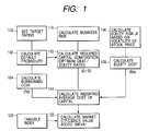
- Fig. 1 is a flowchart of computer processing performed by a business performance index processing system according to an embodiment of the present invention.
- the cost of capital is calculated as described below.
- the invested capital is therefore the sum of a fund (debt) raised as the money borrowed from financial institutions or the like and issued bonds, and a fund (equity) raised as the capital stock obtained as a result of issuing stocks or the like and retained earnings or the like. It represents a fund that is needed to set up and carry out the business. Further, it is necessary to pay a source of the fund the cost that corresponds with the business, that is, the cost of capital.
- the ratio of the cost of capital to the invested capital is the weighted average cost of capital.
- Cost of Capital Weighted Average Cost of Capital x Invested Capital
- the borrowing cost refers to an interest rate of borrowings
- the equity cost refers to an expected return on equity demanded by stockholders, such as dividends paid to stockholders or an increase in retained earnings.
- the weighted average cost of capital can be calculated by obtaining a weighted average of the borrowing cost and the equity cost in terms of the capital composition.
- the capital invested in a specific business unit represents a share of the total invested capital appropriated for that particular business unit out of the total invested capital of the enterprise.
- the weighted average cost of capital of each individual business unit is therefore not constant.
- the following method is therefore employed to virtually divide the invested capital for each business unit into debt and equity, thereby obtaining the weighted average cost of capital of each. This weighted average cost of capital is then used to arrive at the cost of capital.
- the borrowing cost is first calculated.
- Calculation of the borrowing cost proceeds as follows. First of all, default probability and borrowing cost values associated with different credit ratings are established as shown in Fig. 3 using a database that stores therein past default records, actual market standings, and the like.
- a target rating of the business unit to be evaluated is set in step 100
- the default probability of the business unit concerned is determined in step 102
- the borrowing cost (Rd) of the business unit concerned is determined in step 104.
- the equity cost represents the cost for the equity (dividends to be paid to stockholders or an increase in retained earnings).
- Calculation of the equity cost (Re) proceeds as follows.
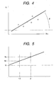
- an equity risk index ⁇ is calculated using past data of the return of the target enterprise (Ri) (or the per share earning ratio of a company in the same industry, if the target enterprise is not listed) and the return of a stock market (Rm) (for example, TOPIX), as shown in Fig. 4 .
- the equity cost (Re) is then calculated in step 108.
- the equity cost (Re) is obtained from a diagram, as shown in Fig. 5 , in which the horizontal axis represents values of the equity risk index ⁇ , while the vertical axis represents the return (R).
- the per share earning ratio of the stock market for example, TOPIX
- Rm when the equity risk index ⁇ is 1.0.
- Rf a rate of return on risk-free assets
- the per share earning ratio when the equity risk index obtained in Fig. 4 is ⁇ is the equity cost (Re).
- Calculation for the required capital composition (an optimum debt/equity ratio) is next performed. It is obtained from the default probability (e.g., 0.1%) determined in step 102 and a business risk.
- the business risk can be represented by a stochastic distribution of the ratio (ROI, or Return on Investment) of the value of profit (operating profit) to the invested capital (the invested amount of money).
- Fig. 2 in which the horizontal axis represents ROI values (%) and the vertical axis represents a probability frequency.
- the horizontal axis represents ROI values (%) and the vertical axis represents a probability frequency.
- the default probability e.g. 0.8%
- the capital composition the debt/equity ratio
- This capital composition therefore fluctuates depending on the business risk (ROI distribution) and a set target credit rating (that is, the default probability).
- the ROI distribution curve shown in Fig. 2 assume that the entire area defined by the ROI distribution curve is 1. Focusing only on an extreme end of the negative ROI value as data of immediate concern allows to find the ROI distribution point, at which the area of the chart is 0.1%. The area of chart of 0.1% indicates that there is an only 0.1% probability of a loss increasing than this.
- the ROI value corresponding to the area of 0.1% may be, for example, -40%. This means that, for an enterprise (business) having an ROI distribution as shown in Fig. 2, the equity accounts for 40% of the invested capital (debt + equity). It therefore follows that, for an enterprise (business) having an ROI distribution curve as shown in Fig. 2, it is necessary that the equity accounts for 40% of the invested capital in order to set the default probability at 0.1%.
- step 120 the net operating profit after tax is obtained according to accounting rules.
- step 122 the MEVA is calculated as detailed below using the weighted average cost of capital calculated in step 114.
- Market Efficiency Value Added (Net Operating Profit after Tax/Invested Capital - Weighted Average Cost of Capital) x Invested Capital
- a Marginal Accumulated Discounted-MEVA is calculated in order to measure a marginal effect of an individual business in an enterprise-wide portfolio.
- AD-MEVA ⁇ ⁇ MEVAt/(1 + r) t-s ⁇ where, t: period to be evaluated; s: reference period for evaluation; MEVAt: MEVA record for period t; r: risk-free rate (government bond rate or the like) or weighted average cost of capital.
- each MEVA can be expressed as follows based on equation (1).
- MEVA A Net Operating Profit after Tax A - Cost of Capital A
- MEVA B Net Operating Profit after Tax B - Cost of Capital B
- MEVA C Net Operating Profit after Tax C - Cost of Capital C
- MEVA X Net Operating Profit after Tax X - Cost of Capital X
- Net Operating Profit after Tax X Net Operating Profit after Tax A + Net Operating Profit after Tax B + Net Operating Profit after Tax C
- Cost of Capital X Cost of Capital A + Cost of Capital B + Cost of Capital C
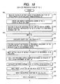
- the system shown in Fig. 16 is what is called a computer system, comprising an input unit 170, an output unit 172, a processing unit 174, a temporary storage unit 176, a transmitter/receiver unit 178, and a storage unit storing various types of data files 180 to 188, all connected to a bus 192.
- the input unit 170 is an input means of a known personal computer, or PC, provided with keys for data entry or a mouse. It may further include a reader for a recording medium such as a CD.
- the output unit 172 is a display device of the PC and a printer.
- the processing unit 174 may be a processor of the PC or that of a server.
- the temporary storage unit 176 is a main memory of the PC or a server. This system may be connected by way of the transmitter/receiver unit 178 to an external computer system through a public network such as the Internet.
- the data file 180 stores therein a table of credit ratings relating to corresponding default probability and borrowing cost values shown in Fig. 3.
- This table is generally created as follows. Namely, credit rating data and default probability data which are disclosed by credit-rating firms are purchased and input through the input unit 170.
- the borrowing cost data is purchased from banks in a form created by the banks and input through the input unit 170.
- the processing unit 174 edits and processes the data input through the input unit 170 and the resultant processed data is stored in memory as the data file 180.
- the data file 182 stores therein stock price data.
- the data file 184 stores data on ROI/probability distribution shown in Fig. 2.
- the data file 186 stores files of ROI.
- the data file 188 stores the business management data.
- the tabulated data of Fig. 3 is read from the data file 180 for setting of credit rating and displayed on the output unit 172 (302).
- the credit rating is then input through the input unit 170. It is temporarily stored in the temporary storage unit 176 (304).
- the processing unit 174 next calculates the default probability from the tabulated data of Fig. 3. The result thereof is temporarily retained in the temporary storage unit 176 (102).
- the processing unit 174 then calculates the borrowing cost from the tabulated data of Fig. 3.
- Step 106 To calculate the equity risk ⁇ from volatility of the stock prices (step 106), volatility of past Tokyo stock prices and that of the stock prices to be evaluated are obtained from an external database through the transmitter/receiver unit 178 (312). While this data is stored in the data file 182, the processing unit 174 not only creates the distribution graph shown in Fig. 4 to display it on the output unit 172, but also displays the ⁇ value plotted on the graph (314). The ⁇ value plotted on the graph is validated by operating a return key on the display screen. This value is stored in the temporary storage unit 176. For the calculation of the equity cost (step 108), the processing unit 174 calculates the equity cost (Re) (320) after Rf has been input (318).
- the processing unit 174 calculates the ROI probability distribution shown in Fig. 2 using the historical method or the simulation method, and creates the graph of Fig. 2 (110).
- the processing unit 174 calculates the required capital composition based on the result of calculation of the business risk (110) and the default probability (102). The processing unit 174 then calculates the weighted average cost of capital according to equation (5) (114). The unit 174 further calculates MEVA using data of profit after tax acquired from the data file 188 or a tangible index such as the peak value shown in Fig. 2 entered (120). This calculation is performed in accordance with equations (8), (9), (10), and (11) (Step 122). The processing unit 174 creates the graph shown in Fig. 6 and subsequent ones to show the result of the calculations performed and makes the display device of the output unit 172 display it.
- the results of the calculations performed by the processing unit 174 are temporarily stored in the temporary storage unit 176 at different stages in the middle of calculation processes before the output is provided for the display. Those who are involved with a business performance evaluation make an investment decision by studying the graph that is displayed.
- MEVA for a single fiscal year and cumulative MEVA for each year for each business unit are displayed as shown in Fig. 6.
- the line graph shown in Fig. 6 represents numeric values of MEVA of each single fiscal year, while the bar graph shown in Fig. 6 represents the cumulative value thereof. Displaying both the line graph showing changes in the value of single fiscal year and the bar graph showing changes in the cumulative value makes it possible to even more appropriately identify performance of the business unit concerned. When more periods elapse to allow actual values of MEVA to be measured, it becomes possible to display in a bar graph the record values or cumulative values thereof in comparison with the original forecast values or cumulative values thereof.
- a specific business unit for which the displayed data is intended, can be selected by dropping down a key marked with "Business Unit A” being displayed in the display shown in Fig. 6.
- the discount rate applicable to aggregating can also be selected by dropping down a key for the discount rate and selecting, for example, "risk-free rate.”
- the reference point for evaluation is also selectable by dropping down a key for the evaluation reference point in Fig. 6 and selecting, for example, the "2nd Period.”
- Segment of data in the display of MEVA may also be selectively displayed, either individually for the total of all businesses, each business unit (business A, business B, business C, ...), and for each project to be invested (project a, project b, project c, %), or collectively for comparison among a plurality of segments.
- the calculation period for MEVA may be annual, semi-annual, quarterly, or monthly and the display can be given for each period of calculation basis.
- FIG. 6 A display example shown in Fig. 6 is used by those who make an investment decision and those who formulate an investment plan when they attempt to measure the business value of the investment plan in question and use as bases for making a decision as to whether or not to invest in the business. As time elapses after the investment plan has been formulated to allow actual values to be measured, Fig. 6 may also be used for comparison and verification against the forecast values projected when the plan was first formulated.
- Fig. 7 displays a comparison between the forecast and record values of MEVA, and a verification and deviation analysis between the two.
- the forecast and record values of MEVA shown in Fig. 6 are tabulated according to the period.
- Fig. 7 also gives data for the invested capital, sales, net operating profit after tax, and weighted average cost of capital that are required when calculating the MEVA in question. It displays the forecast and record values side by side and gives a difference between the two for each of these parameters, thus allowing a difference analysis for each to be made easily.
- Fig. 8 shows a screen that displays a business risk of a particular business unit. Specifically, the horizontal axis represents the net operating profit after tax, while the vertical axis represents frequencies of corresponding values of the net operating profit after tax occurring.
- Fig. 8 is a diagram showing distribution of net operating profit after tax values tallied up for the entire period of a business plan for business unit A.
- the specific business for which data is to be displayed, may nonetheless be selected by dropping down the box of the business unit name.
- the data may also cover a specific business plan or an entire enterprise, in addition to the specific business unit.
- the target rating moves horizontally to the right or left accordingly across it when the rating of "A,” “BBB,” or the like or the default probability of 0.01% or the like is entered, or selected from the rating/default probability table shown in the screen.
- clicking different parts of the screen as shown in Fig. 8 will display different numeric values as detailed in the following.
- Fig. 9 is a typical screen that displays a list of major financial statements figures (invested capital, sales, net operating profit after tax, cost of capital, MEVA, stockholders' equity, internal capital, and the difference in capital) of each business or all businesses.
- the recalculation button provided on the display screen of Fig. 9 is used to change the financial statements figures in the screen or to recalculate the figures before and after correlation of all businesses are taken into consideration after figures involved with a new business have been entered.
- the screen shown in Fig. 9 not only facilitates a comparative examination of each individual business, but also is used to determine how a new business, when it is carried out, affects figures of all other businesses. Clicking [Back] in the display screen shown in Fig. 9 will cause the screen shown in Fig. 8 to reappear. Clicking [Next] in the screen shown in Fig. 9 will show the screen shown in Fig. 10.
- Fig. 10 is a diagram that shows a typical screen displaying, in a graph, the relationship between the MEVA and invested capital (debt + equity) according to the business unit (to be invested). It covers all business units to show the relationship between MEVA and invested capital. Although the display screen shown in Fig. 10 covers all business units, it is possible to selectively set a specific business unit by dropping down the box for the business unit.
- FIG. 10 for the invested capital given on the horizontal axis, that of all businesses up to business G is equivalent to the total invested capital of the enterprise.
- the vertical axis represents the MEVA of a single fiscal year (or the cumulative MEVA).
- Point a depicts the invested capital and MEVA involved with business A
- point b depicts the invested capital and MEVA involved with business B in relation to point a set up as the reference point.
- point c represents the invested capital and MEVA involved with business C
- point d represents those involved with business D.
- point E since the MEVA value thereof is negative, point e is located downwardly on the right of point d.
- the MEVA of the entire enterprise is negative.
- Fig. 10 tells that, while each of the businesses A, B, C, and D works to increase the MEVA of the entire enterprise, each of the businesses E, F, and G works to decrease the MEVA of the entire enterprise. Moving the cursor to each of the different businesses on the graph will display "MEVA xx billion yen (ratio to the total of all MEVA values) and invested capital xx billion yen (ratio to the total of all invested capitals)" of that particular business. Further, double-clicking a specific business will display the MEVA and other values of that particular business in the format shown in Figs. 6, 7, and 8. Clicking [Back] in the display screen shown in Fig. 10 will cause the screen shown in Fig. 9 to reappear. Clicking [Next] in the screen shown in Fig. 10 will show the screen shown in Fig. 11.
- Fig. 11 is a diagram that shows a typical screen displaying risk and return values of each business and the entire enterprise.
- the display screen also shows a composition of different businesses that realizes an expected return with the minimum risk (an effective frontier) as selected from among the existing businesses.
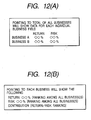
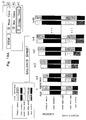
- pointing to total of all businesses will display data (return: XX%; risk: XX%) for each individual business field as shown in Fig. 12A. Clicking each business in the display screen shown in Fig. 11 will jump to the display screen shown in Figs. 6 and 7 for the specific business.
- pointing to each business will display "return: XX% (ranking among all businesses); risk: XX% (ranking among all businesses); and contribution (return/risk ranking)" as shown in Fig. 12B.
- the [Recalculation] button is clicked.
- pointing to the effective frontier curve in the display screen as shown in Fig. 11 will display the percentage distribution of businesses shown in Fig. 13.
- Fig. 13 is a diagram that shows a typical screen displaying percentage distribution of businesses on the effective frontier.
- the horizontal axis represents values of the return (ROI) and the graph shows changing percentage distributions of businesses with varying return values.
- ROI return
- pointing to the effective frontier curve on the display screen shown in Fig. 11 will display a graph showing the percentage distributions of businesses on the effective frontier as shown in Fig. 13.
- a specific return value on the horizontal axis for example, a return value of 3.7%) provides the specific percentage distributions of different businesses as detailed in the following. Namely, business A is 15%, business B is 10%, business C is 5%, business E is 70%, and business D is 0%.
- a return value of 4.7%) provides the specific percentage distributions of different businesses as follows: namely, business A is 20%, business B is 15%, business C is 15%, business E is 40%, and business D is 10%. This means that selecting a specific return value will give specific percentage distributions of different businesses that allow to stably achieve a target. Clicking [Back] in the display screen shown in Fig. 13 will cause the screen shown in Fig. 11 to reappear. Clicking [Quit] in the screen shown in Fig. 13 will close the screen shown in Fig. 13, causing the initial screen shown in Fig. 6 to reappear.
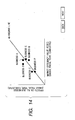
- Fig. 14 is a diagram that shows a typical screen displaying MEVA of each business and an effect of the business in question on the MEVA value of the entire enterprise (increased or decreased effect of MEVA). Specifically, the balance in the MEVA value of the entire enterprise between that including the business in question and that excluding the same is obtained to determine contribution of the business concerned. This serves as a reference when starting a new business and considering the effect of the new business on the existing businesses.
- the horizontal axis represents the MEVA of each business, while the vertical axis represents the effect on all businesses (Marginal Accumulated Discounted-MEVA, or MAD-MEVA).
- the screen shows this relationship for each business.
- the effect on all businesses means the degree of how much the addition of the business in question to the business portfolio increases the cumulative discounted value of the MEVA of the business portfolio. If the point of a specific business is located above the 45-degree line, it is known that the specific business in question contributes to the business value of the entire enterprise more than the value of the specific business.
- the display serves as a reference for making a decision that ensures even more efficient business operations, while taking into consideration diversification effect and synergy effect. Clicking [Back] in the display screen shown in Fig. 14 will cause the screen shown in Fig. 13 to reappear.
- Fig. 15 is a diagram that shows a typical screen displaying, in a table, an accumulated discounted value of MEVA of each business and an effect (marginal accumulated discounted value) of the business in question on the entire enterprise, that is Marginal Accumulated Discounted-MEVA or MAD-MEVA, shown in Fig. 14.
- Preparing an at-a-glance table facilitates a comparative analysis between different pairs of businesses. It serves as a primary source of decision-making for building an even more efficient business portfolio. They are other cases of embodiments.
- Fig. 6 explained previously shows the graph which displayed on the display the progress mouth, the actual result value, and the reexamination plan value of MEVA. In this figure 6, if the numerical value which shows other management states, for example, the numerical value of balance sheet (state of property and a debt, and capital) or cash flow, can be displayed on a display, it will be great help to a manager.
- Fig. 6 did not explain, if operation of changing the contents of a display is performed by operating a change button etc., it will change to the graph of the data chosen from the graph about MEVA currently displayed in Fig. 6. For example, when balance sheet is chosen by operation of the above-mentioned change button, the graph of the balance sheet shown in figure 19A or figure 19B is displayed on the display. Moreover, if cash flow is chosen as a change of the graph about MEVA, the graph of the cash flow shown in figure 19C or figure 19D will be displayed on a display.
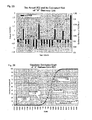
- Figure 19A is the figure which displayed the graph of the average case of the range of fluctuation when predicting the future of the state of the selected property for every enterprise fiscal year and the selected debt, and capital.
- Figure 19B is the figure which displayed the graph of the bad case of fluctuation when predicting the future of the state of the selected property for every enterprise fiscal year and the selected debt, and capital. It is the figure which displayed the graph which shows the state of the prediction value of the cash flow for every fiscal year of the selected enterprise.
- Figure 19C is the figure which displayed the graph of the average case of fluctuation when predicting the state of the cash flow for every fiscal year of the selected enterprise in consideration of the range of fluctuation.
- Figure 19D is the figure which displayed the graph of the bad case of the ranges of fluctuation when predicting the state of the cash flow for every fiscal year of the selected enterprise in consideration of the range of fluctuation.
- deflection width exists in the prediction value by which the simulation was carried out.
- the portion of the good state of the domain of deflection width was chosen and it was shown in graph, and when the portion of a bad state is chosen, in the case where an average domain is chosen, the numerical values of a prediction value differ and the graph displayed differs.
- the operation area 12 has the function which chooses the portion of the good state of the domain of the above-mentioned deflection width, the portion of a bad state, and an average portion.
- the present display value shows in which state of a prediction value, i.e., which portions of the portion of a good state, the portion of a bad state, and an average portion.
- Figure 19A and figure 19C Since 1 ⁇ Average 14 is chosen, displaying the graph of the average value of the deflection width of a simulation result is shown.
- selection of 3 ⁇ Worst 18 displays the graph based on the numerical value of the bad portion of the domain of the above-mentioned deflection width. They are figure 19B and figure 19C. If 2 ⁇ BEST 16 is chosen, the graph based on the numerical value of the good portion of the domain of the above-mentioned deflection width is displayed.
- Fig. 20 is the flow chart of a system of operation, and MEVA, balance sheet, and cash flow are calculated at Steps 22-26, and it is keeped by the memory.
- Step 28 if the contents which should be displayed on a display are chosen (for example, if the data of the data of Fig. 6, the data of figure 19 A/B, or figure 19 C/D is chosen) (Step 28), selected data will be read and it will indicate by graph (Step 30).
- the graph in 1 ⁇ Average mode is displayed as a typical display. For example, the graph of figure 19A or figure 19C is displayed.
- Step 32 If the selection button 12 for a display is chosen at Step 32 and 2 ⁇ Vest mode (Step 36) and 3 ⁇ Worst mode (Step 28) are chosen further, the graph in the selected mode will be expressed as Step 42 or Step 44. Moreover, if 1 ⁇ Average is chosen in the state of changing the mode for a display at Step 32 (Step 34), the graph in 1 ⁇ Average mode will be expressed as Step 40.
- These mode selections are already performed by selection of the operation buttons 14, 16, and 18 of the operation area 12 of above-mentioned figure 19 A-D.
- Fig. 21 is a system flowchart showing monthly performance and risk by business unit. The objectives are to manage the business portfolio and to issue alarm. Input data are as follows.
- Step460 corresponds with Fig. 1. And this process calculates WACC by business unit.
- This process uses business risk (ROI distribution) that is calculated with the trend-cycle series of ROI in DB414. And it stores calculated WACC by business unit in DB420. (See Fig. 1's explanation for detail).
- This process uses WACC in DB420 and invested capital and operating profit by business unit in DB402 and stores each trend-cycle series into DB412.
- Step458 uses MAPT analysis (depended variable: actual ROI, explanatory variable: fluctuations of macro index) and calculates each macro indexes exposure and specific ROI (not explained by macro indexes) by business unit.
- This step uses the seasonally adjusted series of ROI (TC + I) in DB414 and actual macro indexes in DB404. This process calculates X j and ⁇ +e i .
- (ROI) i X 1 ⁇ F 1i +X 2 ⁇ F 2i + ⁇ +X n ⁇ F ni + ⁇ +e i
- (ROI) i seasonally adjusted ROI at time i
- F ji fluctuation in actual j macro index at time i
- X j is j macro index exposure and ⁇ +e i is Specific ROI
- this process calculates the covariance matrix among the macro indexes.
- COV ij COV(F i , F j ) where COV ij is (i, j)-component of covariance matrix, COV(F i , F j ) is covariance between fluctuations of i macro index and j macro index.
- Calculated value is stored in DB418 as "Base Information for Estimated Risk Data".
- Step462 uses AR analysis and estimates the expected operating profit and the expected MEVA and the expected ROI by business unit. This process uses operating profit, MEVA and trend-cycle of actual operating profit in DB412, and trend-cycle of actual ROI in DB414. The estimated value is stored in DB422.
- Step466 estimates expected ROI using MR analysis. This step uses each macro indexes exposure by business unit in DB418 and forecast of each macro indexes in DB406.
- Expected ROI X 1 ⁇ F 1 + X 2 ⁇ F 2 + ⁇ + X n ⁇ F n + ⁇ where F j is forecasted fluctuation in j macro index.
- Estimated value is stored in DB422.
- Step468 calculates the estimated ROI distribution using Monte Carlo simulation. This step uses the estimated ROI risk in DB424 and the expected ROI, the expected operating profit and the expected MEVA in DB422. Estimated ROI distribution is stored in DB425.
- Step470 corresponds with Fig. 1.
- This step calculates WACC by business unit using estimated ROI distribution in DB425. (See Fig. 1's explanation for detail)
- Step 472 calculates the achieve probability (*) and the loss probability. This step uses the planed operating profit and loss by business unit in DB408 and invested capital by business unit in DB402. Calculated values are stored in DB426.
- Fig. 22 is the system flowchart showing monthly performance and risk on entire business. The objects are to manage to business portfolio and issue alarm. Input data are as follows.
- Step550 makes efficient frontier with expected ROI and estimated ROI risk.
- This step uses expected ROI by business unit in DB418 and Base Information for Estimated Risk Data in DB 418. And this step uses estimated ROI risk by business unit in DB424 and invested capital by business unit in DB406, and draws the present business portfolio position and each business unit position in a graph.
- the point of efficient frontier (expected ROI and estimated ROI risk's plot) and the point of present business portfolio position and the point of business unit position are stored in DB500.
- Step554 calculates marginal influence that each business gives portfolio (marginal MEVA). This step uses actual operating profit and invested capital by business unit in DB402, WACC based on past record in DB420, WACC based on estimated value in DB428, expected operating profit and expected MEVA in DB422. Calculated value is stored in DB504. (See Fig. 32's explanation for detail).
- Step556 makes MEVA Frontier. This step uses WACC based on past record in DB420, WACC based on estimated value in DB428 , expected ROI by business unit in DB422 and actual ROI by business unit in DB402. Calculated value is stored in DB502. (See Fig. 28's explanation for detail).
- Step558 analyzes style of business portfolio. This process uses each macro indexes exposure by business unit in DB418 and invested capital by business unit in DB402. Calculated value is stored in DB508. (See Fig. 30, 31's explanation for detail).
- Fig. 23 shows a line graph and a bar graph.
- horizontal axis is Year Month
- vertical axis is operating profit.
- a bar graph is monthly operating profit of "A" business unit.
- a line graph is seasonally adjusted operating profit of "A" business unit.
- Input data is actual operating profit in DB402 of Fig. 21 and trend-cycle of operating profit (TC) in DB412 of Fig. 21.
- a line graph (trend-cycle of operating profit) contributes to see trend of operating profit for long term because actual operating profit usually has big fluctuations.
- This graph also contains expected operating profit and its risk that is estimated by AR Analysis in DB422. So it is possible to see the fluctuations of operating profit in the future.
- Fig .24 shows a line graph and a bar graph.
- horizontal axis is Year Month; vertical axis is ROI (%).
- a bar graph is monthly actual ROI.
- a line graph is trend-cycle of actual ROI.
- a line graph (trend-cycle of ROI) contributes to see the trend of ROI for long term because actual ROI usually has big fluctuations.
- This graph also contains expected ROI and its risk that is estimated by AR Analysis and MR Analysis in DB422. So it is possible to see the fluctuations of ROI in the future and to compare different estimated method: AR analysis and MR analysis.
- Fig. 25 shows a line graph and a bar graph.
- horizontal axis is Year Month; left vertical axis is actual ROI (%); right vertical axis is estimated ROI risk (standard deviation %).
- a bar graph is monthly actual ROI.
- a line graph is estimated ROI risk.
- Fig. 26 shows a line graph and points of three probabilities.
- horizontal axis is ROI (%); vertical axis is cumulative probability (%).
- a line graph is cumulative distribution graph of "A" business unit's ROI. Three points are achieve probability, default probability and loss probability. Input data are the achieve probability and the loss probability by business unit in DB 426 of Fig. 21. To get grasps of various risk at a time is possible, because this graph contains various probabilities.
- Fig. 27 is a graph showing efficient frontier of business portfolio's ROI.
- horizontal axis is estimated risk of ROI (standard deviation %); vertical axis is expected ROI (%).
- Input data is efficient frontier data in DB500 of Fig. 22. This graph is indicator of business portfolio's rearrangement, because it is possible to compare each business unit positions, present portfolio position and theoretically optimal business portfolio position in this graph.
- Fig. 28 is a graph showing a bubble chart.
- horizontal axis is WACC (%); vertical axis is ROI (%); bubble size is invested capital.
- Input data is MEVA Frontier data in DB502 of Fig. 22. This graph expresses relationship WACC and ROI. It is possible to check on an appropriate WACC, because we can compare expected ROI, actual ROI and WACC in this graph.
- Fig. 29 shows a bar graph of contribution value (macro index exposure ⁇ fluctuations in macro index) and a line graph of fluctuations in macro index.
- left vertical axis is contribution value for ROI; right vertical axis is fluctuations in macro index; horizontal axis is Year Month.
- Input data is contribution data in DB506 of Fig. 22. This graph gives important indicator on past analysis that how large fluctuations in macro index should have contributed fluctuations in ROI on entire business.
- Fig. 30 is a graph showing a bubble chart.
- vertical axis is "A" macro index exposure
- horizontal axis is "B” macro index exposure
- bubble size is invested capital.
- Input data is exposure data in DB508 of Fig. 22. It makes possible the present analysis of the business portfolio style: macro index exposure by business unit and invested capital in one graph.
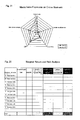
- Fig. 31 is graph showing a radar chart.
- items are macro index's names and values are macro index exposures.
- This graph has two radar lines at different time point.
- Input data is exposure data in DB508 of Fig. 22. It is possible to get a grasp of style of different time by comparing between different point's macro index exposures in this graph.
- Fig. 32 is a table showing MEVA based on past record, MEVA based on forecast of operating profit and marginal influence that business unit gives portfolio.
- Input data is DB504 of Fig .22. This table contributes to compare different business unit, because it is on the same table. And it is possible to get information for purpose of constructing efficient business portfolio.
- the business performance index processing system can accomplish the following task. Namely, it provides business performance indices that relate to the management of performance evaluation, incorporate a risk (uncertainty) evaluation in the investment and withdrawal guidelines, appropriately create a business portfolio (selection and concentration), make the invested capital-to-debt composition (financing) appropriate, and eventually bring a sustainable growth to . the company in harmony with the society.
- the calculation system of the present invention it is possible to vitalize operations within a company, determine investment or withdrawal for each business unit to concentrate on specific areas of businesses, ensure optimum corporate finance, and thereby allow the company to maintain the sustainable growth in harmony with the society.
Landscapes
- Business, Economics & Management (AREA)
- Engineering & Computer Science (AREA)
- Accounting & Taxation (AREA)
- Finance (AREA)
- Development Economics (AREA)
- Strategic Management (AREA)
- Economics (AREA)
- General Business, Economics & Management (AREA)
- Physics & Mathematics (AREA)
- Marketing (AREA)
- General Physics & Mathematics (AREA)
- Theoretical Computer Science (AREA)
- Human Resources & Organizations (AREA)
- Entrepreneurship & Innovation (AREA)
- Technology Law (AREA)
- Game Theory and Decision Science (AREA)
- Operations Research (AREA)
- Educational Administration (AREA)
- Quality & Reliability (AREA)
- Tourism & Hospitality (AREA)
- Financial Or Insurance-Related Operations Such As Payment And Settlement (AREA)
Abstract
A computer is used to perform the calculations for obtaining: a capital composition corresponding to a predetermined default probability based on a probability distribution of a return on investment; a weighted average cost of capital based on the capital composition, a borrowing cost, and an equity cost; and a market efficiency value added from the weighted average cost of capital and a net operating profit after tax. The market efficiency value added obtained through these calculations is then displayed appropriately so as to provide support in decision-making. This provides support in decision-making for determining investment or with drawal for each business unit to concentrate on specific areas of businesses, ensuring optimum business operations, and thereby allowing an enterprise to maintain a sustainable growth in harmony with the society. <IMAGE>
Description
Patent Application Serial No. 10/227,796
The present invention relates to a business
performance index processing system. More particularly, it
relates to displaying, through calculations performed by a
computer for business performance-related indices and based
on the results of these calculations, an item related to
measurement of performance of an entire enterprise or
business units the enterprise has therein, or a new
business to be started.
In recent years, the business circumstances
surrounding enterprises have become more and more severe
and it has become important to even more properly evaluate
each business of an enterprise and to appropriately
evaluate the future of a new business planned so as to meet
the requirement of both the stockholders (investors) and
creditors.
Various performance measurement methods are
currently examined and applied to making a business
performance evaluation. Nonetheless even more appropriate
displaying method is desired.
An object of the present invention is to provide a
business performance index processing system that performs
calculations through an appropriate method for obtaining
market efficiency value added (MEVA) that can be used as an
index for evaluation of business performance and displays
the results of the calculations.
Another object of the present invention is to
provide a system capable of displaying appropriately a
business value in a format that helps make a decision in
terms of management of an enterprise.
Other objects of the present invention will be
described in the preferred embodiments of the invention to
be described later.
To achieve the foregoing objects, the business
performance index processing system according to the
preferred embodiments of the present invention performs
calculations for obtaining the following three parameters
based on a probability distribution of the ratio of the
value of profit to the investment amount (ROI). The three
parameters are: a capital composition (debt/equity ratio)
that satisfies a predetermined default probability; a
weighted average cost of capital based on the capital
composition, and a borrowing cost and an equity cost; and,
market efficiency value added, or MEVA, from the weighted
average cost of capital based on a net operating profit
after tax. Based on the results of these calculations, it
thereby produces an output of an appropriate form, and
gives a display, of indices that serve as the basis for
making a managerial decision.
The invention is characterized in a number of
aspects to be described in the preferred embodiments of the
invention to be described later.
Other objects and advantages of the invention will
become apparent from the following description of
embodiments with reference to the accompanying drawings in
which:
The calculations performed to obtain market
efficiency value added, or MEVA, that serves as a business
performance index and display thereof in the business
performance index processing system according to the
present invention may find applications in the following.
Namely, it may be applicable to a value analysis, in which
it is decided whether or not to invest in a new business to
be started. It may also appropriately be applicable to
determining whether or not an entire enterprise or a
specific existing business unit is efficient or dynamic and
revitalized enough.
Fig. 1 is a flowchart of computer processing
performed by a business performance index processing system
according to an embodiment of the present invention.
The MEVA is calculated as follows. It is calculated
by subtracting a cost of capital invested in a business
from a profit earned by the business. Namely, it is
expressed as:
Market Efficiency Value Added = Net Operating Profit
after Tax - Cost of Capital
The net operating profit after tax is a net profit before
interest after tax as calculated according to accounting
rules.
The cost of capital is calculated as described below.
The invested capital is, to begin with, expressed as:
Invested Capital = Debt + Equity
The invested capital is therefore the sum of a fund (debt)
raised as the money borrowed from financial institutions or
the like and issued bonds, and a fund (equity) raised as
the capital stock obtained as a result of issuing stocks or
the like and retained earnings or the like. It represents
a fund that is needed to set up and carry out the business.
Further, it is necessary to pay a source of the fund the
cost that corresponds with the business, that is, the cost
of capital. The ratio of the cost of capital to the
invested capital is the weighted average cost of capital.
Namely, it is expressed as:
Cost of Capital = Weighted Average Cost of Capital x
Invested Capital
The cost of capital may be divided into a portion involved
with debt and a portion involved with equity. Namely, it
is expressed as:
Cost of Capital = Borrowing Cost x Debt + Equity
Cost x Equity
The borrowing cost refers to an interest rate of
borrowings, and the equity cost refers to an expected
return on equity demanded by stockholders, such as
dividends paid to stockholders or an increase in retained
earnings. The weighted average cost of capital may be
expressed by dividing each of both sides of (4) by the
invested capital. Namely, it is expressed as:
Weighted Average Cost of Capital = Borrowing Cost x
(Debt/Invested Capital) + Equity Cost x (Equity/Invested
Capital)
The weighted average cost of capital can be calculated by
obtaining a weighted average of the borrowing cost and the
equity cost in terms of the capital composition.
When the weighted average cost of capital is
calculated and the cost of capital can be obtained, it then
becomes possible to calculate MEVA using equation (1).
From the viewpoint of an entire enterprise, the
borrowing cost and an equity ratio are determined
efficiently in the market, which allows the cost of capital
to be calculated relatively easily.
Assume, on the other hand, that it is attempted to
calculate the cost of capital of each business unit within
an enterprise. The capital invested in a specific business
unit represents a share of the total invested capital
appropriated for that particular business unit out of the
total invested capital of the enterprise. The weighted
average cost of capital of each individual business unit is
therefore not constant. The following method is therefore
employed to virtually divide the invested capital for each
business unit into debt and equity, thereby obtaining the
weighted average cost of capital of each. This weighted
average cost of capital is then used to arrive at the cost
of capital.
Referring to Fig. 1, the borrowing cost is first
calculated.
Calculation of the borrowing cost proceeds as
follows. First of all, default probability and borrowing
cost values associated with different credit ratings are
established as shown in Fig. 3 using a database that stores
therein past default records, actual market standings, and
the like. When a target rating of the business unit to be
evaluated is set in step 100, the default probability of
the business unit concerned is determined in step 102, and
the borrowing cost (Rd) of the business unit concerned is
determined in step 104.
Calculation of the equity cost of the business unit
concerned is then performed. The equity cost represents
the cost for the equity (dividends to be paid to
stockholders or an increase in retained earnings).
Calculation of the equity cost (Re) proceeds as follows.
In step 106, an equity risk index β is calculated using
past data of the return of the target enterprise (Ri) (or
the per share earning ratio of a company in the same
industry, if the target enterprise is not listed) and the
return of a stock market (Rm) (for example, TOPIX), as
shown in Fig. 4. The equity risk index β can be obtained
using the following equation:
β = (covariance between the stock price and
TOPIX)/(variance of TOPIX)
The equity cost (Re) is then calculated in step 108.
The equity cost (Re) is obtained from a diagram, as shown
in Fig. 5, in which the horizontal axis represents values
of the equity risk index β, while the vertical axis
represents the return (R). Referring to Fig. 5, assume
that the per share earning ratio of the stock market (for
example, TOPIX) is Rm when the equity risk index β is 1.0.
Assume also that a rate of return on risk-free assets such
as sovereign bonds is Rf. The per share earning ratio when
the equity risk index obtained in Fig. 4 is β is the equity
cost (Re).
Using a capital asset pricing model (CAPM) and the
equation given in the following, the equity cost (Re) is
therefore calculated from Rf and Rm:
Re = Rf + β x (Rm - Rf)
Calculation for the required capital composition (an
optimum debt/equity ratio) is next performed. It is
obtained from the default probability (e.g., 0.1%)
determined in step 102 and a business risk. The business
risk can be represented by a stochastic distribution of the
ratio (ROI, or Return on Investment) of the value of profit
(operating profit) to the invested capital (the invested
amount of money).
Reference is now made to Fig. 2, in which the
horizontal axis represents ROI values (%) and the vertical
axis represents a probability frequency. In the graph
(showing an ROI distribution curve) shown in Fig. 2, a
specific ROI value is identified according to the default
probability (e.g., 0.1%) and the capital composition (the
debt/equity ratio) corresponding to the identified ROI
value is obtained. This capital composition (the
debt/equity ratio) therefore fluctuates depending on the
business risk (ROI distribution) and a set target credit
rating (that is, the default probability).
The following description elaborates on it. In the
ROI distribution curve shown in Fig. 2, assume that the
entire area defined by the ROI distribution curve is 1.
Focusing only on an extreme end of the negative ROI value
as data of immediate concern allows to find the ROI
distribution point, at which the area of the chart is 0.1%.
The area of chart of 0.1% indicates that there is an only
0.1% probability of a loss increasing than this. The ROI
value corresponding to the area of 0.1% may be, for example,
-40%. This means that, for an enterprise (business) having
an ROI distribution as shown in Fig. 2, the equity accounts
for 40% of the invested capital (debt + equity). It
therefore follows that, for an enterprise (business) having
an ROI distribution curve as shown in Fig. 2, it is
necessary that the equity accounts for 40% of the invested
capital in order to set the default probability at 0.1%.
The required capital composition (an optimum
debt/equity ratio) and the weighted average cost of capital
are calculated as described in the foregoing. In step 120,
the net operating profit after tax is obtained according to
accounting rules. In step 122, the MEVA is calculated as
detailed below using the weighted average cost of capital
calculated in step 114.
Market Efficiency Value Added (MEVA) = (Net
Operating Profit after Tax/Invested Capital - Weighted
Average Cost of Capital) x Invested Capital
In the process of obtaining the weighted average cost of
capital, consideration has been given to maintaining
consistency between the bond market and the stock market in
regard to the borrowing cost, equity cost, and the
debt/equity ratio. This makes it possible to calculate a
market efficiency business value.
In step 124, a Marginal Accumulated Discounted-MEVA,
or MAD-MEVA, is calculated in order to measure a marginal
effect of an individual business in an enterprise-wide
portfolio.
When calculating an Accumulated Discounted-MEVA, or
AD-MEVA, an adjustment is made using a "risk-free rate" or
the "weighted average cost of capital" before adding up
MEVA values between different points in time. Specifically,
AD-MEVA = Σ {MEVAt/(1 + r) t-s}
where, t: period to be evaluated; s: reference period for
evaluation; MEVAt: MEVA record for period t; r: risk-free
rate (government bond rate or the like) or weighted average
cost of capital.
The following concept is applied to the measurement
method of the marginal effect. Assuming a business
portfolio X comprising three businesses of A, B, and C,
each MEVA can be expressed as follows based on equation (1).
MEVA A = Net Operating Profit after Tax A - Cost of
Capital A
MEVA B = Net Operating Profit after Tax B - Cost of
Capital B
MEVA C = Net Operating Profit after Tax C - Cost of Capital C
MEVA X = Net Operating Profit after Tax X - Cost of
Capital X
The following relationship holds true between the
net operating profit after tax of each individual business
and the net operating profit after tax of the business
portfolio.
Net Operating Profit after Tax X = Net Operating
Profit after Tax A + Net Operating Profit after Tax B + Net
Operating Profit after Tax C
The relationship between each business and the business
portfolio is as follows in terms of the cost of capital.
Cost of Capital X = Cost of Capital A + Cost of
Capital B + Cost of Capital C
Since it can be expected that a business risk
forming part of the cost of capital is reduced by the
effect of diversification of portfolio, the cost of capital
of the business portfolio can be eventually smaller. From
equations (9) and (10), the following relationship
therefore holds true between each individual business and
the business portfolio in terms of MEVA.
MEVA X ≧ MEVA A + MEVA B + MEVA C
Specifically, as the number of businesses that make
up the business portfolio increases, it becomes more likely
that the MEVA of the entire business portfolio is greater
than the simple addition of MEVA values involved with
individual businesses. An effective business portfolio
management can therefore be implemented by comparatively
examining the MEVA value of each individual business and
the difference in MEVA values between the MEVA value before
and that after the business in question is added (marginal
MEVA).
The system and processing operations thereof will be
described with reference to the system configuration
diagram for implementing a business performance index
processing system shown in Fig. 16 and detailed flowcharts
shown in Figs. 17 and 18.
The system shown in Fig. 16 is what is called a
computer system, comprising an input unit 170, an output
unit 172, a processing unit 174, a temporary storage unit
176, a transmitter/receiver unit 178, and a storage unit
storing various types of data files 180 to 188, all
connected to a bus 192.
The input unit 170 is an input means of a known
personal computer, or PC, provided with keys for data entry
or a mouse. It may further include a reader for a
recording medium such as a CD. The output unit 172 is a
display device of the PC and a printer. The processing
unit 174 may be a processor of the PC or that of a server.
The temporary storage unit 176 is a main memory of the PC
or a server. This system may be connected by way of the
transmitter/receiver unit 178 to an external computer
system through a public network such as the Internet.
The data file 180 stores therein a table of credit
ratings relating to corresponding default probability and
borrowing cost values shown in Fig. 3. This table is
generally created as follows. Namely, credit rating data
and default probability data which are disclosed by credit-rating
firms are purchased and input through the input unit
170. The borrowing cost data is purchased from banks in a
form created by the banks and input through the input unit
170. The processing unit 174 edits and processes the data
input through the input unit 170 and the resultant
processed data is stored in memory as the data file 180.
The data file 182 stores therein stock price data.
The data file 184 stores data on ROI/probability
distribution shown in Fig. 2. The data file 186 stores
files of ROI. The data file 188 stores the business
management data.
Processing for calculation of the borrowing cost
shown in Fig. 1 will be described with reference to Fig. 17.
The tabulated data of Fig. 3 is read from the data file 180
for setting of credit rating and displayed on the output
unit 172 (302). The credit rating is then input through
the input unit 170. It is temporarily stored in the
temporary storage unit 176 (304). The processing unit 174
next calculates the default probability from the tabulated
data of Fig. 3. The result thereof is temporarily retained
in the temporary storage unit 176 (102). The processing
unit 174 then calculates the borrowing cost from the
tabulated data of Fig. 3.
Calculation of the market efficiency value added
(MEVA) will be described with reference to Fig. 18. To
calculate the equity risk β from volatility of the stock
prices (step 106), volatility of past Tokyo stock prices
and that of the stock prices to be evaluated are obtained
from an external database through the transmitter/receiver
unit 178 (312). While this data is stored in the data file
182, the processing unit 174 not only creates the
distribution graph shown in Fig. 4 to display it on the
output unit 172, but also displays the β value plotted on
the graph (314). The β value plotted on the graph is
validated by operating a return key on the display screen.
This value is stored in the temporary storage unit 176.
For the calculation of the equity cost (step 108), the
processing unit 174 calculates the equity cost (Re) (320)
after Rf has been input (318).
For the calculation of the business risk, the
processing unit 174 calculates the ROI probability
distribution shown in Fig. 2 using the historical method or
the simulation method, and creates the graph of Fig. 2
(110).
For the calculation of the required capital
composition (112), when a setting value for the default
probability of the enterprise to be evaluated is entered
through the input unit 170 (322), the processing unit 174
calculates the required capital composition based on the
result of calculation of the business risk (110) and the
default probability (102). The processing unit 174 then
calculates the weighted average cost of capital according
to equation (5) (114). The unit 174 further calculates
MEVA using data of profit after tax acquired from the data
file 188 or a tangible index such as the peak value shown
in Fig. 2 entered (120). This calculation is performed in
accordance with equations (8), (9), (10), and (11) (Step
122). The processing unit 174 creates the graph shown in
Fig. 6 and subsequent ones to show the result of the
calculations performed and makes the display device of the
output unit 172 display it.
The results of the calculations performed by the
processing unit 174 are temporarily stored in the temporary
storage unit 176 at different stages in the middle of
calculation processes before the output is provided for the
display. Those who are involved with a business
performance evaluation make an investment decision by
studying the graph that is displayed.
Displays of various kinds concerning MEVA will be
described. MEVA for a single fiscal year and cumulative
MEVA for each year for each business unit are displayed as
shown in Fig. 6. The line graph shown in Fig. 6 represents
numeric values of MEVA of each single fiscal year, while
the bar graph shown in Fig. 6 represents the cumulative
value thereof. Displaying both the line graph showing
changes in the value of single fiscal year and the bar
graph showing changes in the cumulative value makes it
possible to even more appropriately identify performance of
the business unit concerned. When more periods elapse to
allow actual values of MEVA to be measured, it becomes
possible to display in a bar graph the record values or
cumulative values thereof in comparison with the original
forecast values or cumulative values thereof.
In this display of MEVA, a specific business unit,
for which the displayed data is intended, can be selected
by dropping down a key marked with "Business Unit A" being
displayed in the display shown in Fig. 6. The discount
rate applicable to aggregating can also be selected by
dropping down a key for the discount rate and selecting,
for example, "risk-free rate." The reference point for
evaluation is also selectable by dropping down a key for
the evaluation reference point in Fig. 6 and selecting, for
example, the "2nd Period."
Segment of data in the display of MEVA may also be
selectively displayed, either individually for the total of
all businesses, each business unit (business A, business B,
business C, ...), and for each project to be invested
(project a, project b, project c, ...), or collectively for
comparison among a plurality of segments.
The calculation period for MEVA may be annual, semi-annual,
quarterly, or monthly and the display can be given
for each period of calculation basis.
Clicking each bar of the bar graph shown in Fig. 6
will display data as shown below. Specifically, clicking
the bar for the third period marked with B will display the
following:
A display example shown in Fig. 6 is used by those
who make an investment decision and those who formulate an
investment plan when they attempt to measure the business
value of the investment plan in question and use as bases
for making a decision as to whether or not to invest in the
business. As time elapses after the investment plan has
been formulated to allow actual values to be measured, Fig.
6 may also be used for comparison and verification against
the forecast values projected when the plan was first
formulated.
If any of the record values shown in Fig. 6, for
example, A is clicked, it will display a screen that makes
an analysis of differences from the forecast values (Fig.
7). Specifically, Fig. 7 displays a comparison between the
forecast and record values of MEVA, and a verification and
deviation analysis between the two. In more specific terms,
the forecast and record values of MEVA shown in Fig. 6 are
tabulated according to the period. In addition, Fig. 7
also gives data for the invested capital, sales, net
operating profit after tax, and weighted average cost of
capital that are required when calculating the MEVA in
question. It displays the forecast and record values side
by side and gives a difference between the two for each of
these parameters, thus allowing a difference analysis for
each to be made easily.
Furthermore, if the plan is reviewed at the time of
evaluation, it is possible to display in the screen shown
in Fig. 7 reviewed forecast values in the record value
column after evaluation (for example, at the end of the
second period). This makes it possible to identify the
situation as immediately near as possible.
Clicking [Back] in the display screen shown in Fig.
7 will cause the screen shown in Fig. 6 to reappear.
Clicking [Next] in the screen shown in Fig. 7 will show the
screen shown in Fig. 8.
Fig. 8 shows a screen that displays a business risk
of a particular business unit. Specifically, the
horizontal axis represents the net operating profit after
tax, while the vertical axis represents frequencies of
corresponding values of the net operating profit after tax
occurring. Fig. 8 is a diagram showing distribution of net
operating profit after tax values tallied up for the entire
period of a business plan for business unit A. The
specific business, for which data is to be displayed, may
nonetheless be selected by dropping down the box of the
business unit name. The data may also cover a specific
business plan or an entire enterprise, in addition to the
specific business unit.
In the screen as shown in Fig. 8, the target rating
moves horizontally to the right or left accordingly across
it when the rating of "A," "BBB," or the like or the
default probability of 0.01% or the like is entered, or
selected from the rating/default probability table shown in
the screen. In addition, clicking different parts of the
screen as shown in Fig. 8 will display different numeric
values as detailed in the following. Namely, clicking
stockholders' equity will show "Stockholders' equity: X
billion yen." Clicking profit after tax (expected) will
show "Profit after tax (expected): X billion yen."
Clicking one value of standard deviation will show "1σ: X
billion yen." Clicking probability of profit after tax
being in the positive will show "Probability of profit
after tax being in the positive: X%." Clicking [Back] in
the display screen shown in Fig. 8 will cause the screen
shown in Fig. 7 to reappear. Clicking [Next] in the screen
shown in Fig. 8 will show the screen shown in Fig. 9.
Fig. 9 is a typical screen that displays a list of
major financial statements figures (invested capital, sales,
net operating profit after tax, cost of capital, MEVA,
stockholders' equity, internal capital, and the difference
in capital) of each business or all businesses. The
recalculation button provided on the display screen of Fig.
9 is used to change the financial statements figures in the
screen or to recalculate the figures before and after
correlation of all businesses are taken into consideration
after figures involved with a new business have been
entered.
The screen shown in Fig. 9 not only facilitates a
comparative examination of each individual business, but
also is used to determine how a new business, when it is
carried out, affects figures of all other businesses.
Clicking [Back] in the display screen shown in Fig. 9 will
cause the screen shown in Fig. 8 to reappear. Clicking
[Next] in the screen shown in Fig. 9 will show the screen
shown in Fig. 10.
Fig. 10 is a diagram that shows a typical screen
displaying, in a graph, the relationship between the MEVA
and invested capital (debt + equity) according to the
business unit (to be invested). It covers all business
units to show the relationship between MEVA and invested
capital. Although the display screen shown in Fig. 10
covers all business units, it is possible to selectively
set a specific business unit by dropping down the box for
the business unit.
Referring to Fig. 10, for the invested capital given
on the horizontal axis, that of all businesses up to
business G is equivalent to the total invested capital of
the enterprise. The vertical axis, on the other hand,
represents the MEVA of a single fiscal year (or the
cumulative MEVA). Point a depicts the invested capital and
MEVA involved with business A and point b depicts the
invested capital and MEVA involved with business B in
relation to point a set up as the reference point.
Following this procedure, point c represents the invested
capital and MEVA involved with business C and point d
represents those involved with business D. With business E,
since the MEVA value thereof is negative, point e is
located downwardly on the right of point d. Likewise, when
considering businesses F and G, the MEVA of the entire
enterprise is negative. That is, Fig. 10 tells that, while
each of the businesses A, B, C, and D works to increase the
MEVA of the entire enterprise, each of the businesses E, F,
and G works to decrease the MEVA of the entire enterprise.
Moving the cursor to each of the different businesses on
the graph will display "MEVA xx billion yen (ratio to the
total of all MEVA values) and invested capital xx billion
yen (ratio to the total of all invested capitals)" of that
particular business. Further, double-clicking a specific
business will display the MEVA and other values of that
particular business in the format shown in Figs. 6, 7, and
8. Clicking [Back] in the display screen shown in Fig. 10
will cause the screen shown in Fig. 9 to reappear.
Clicking [Next] in the screen shown in Fig. 10 will show
the screen shown in Fig. 11.
Fig. 11 is a diagram that shows a typical screen
displaying risk and return values of each business and the
entire enterprise. The display screen also shows a
composition of different businesses that realizes an
expected return with the minimum risk (an effective
frontier) as selected from among the existing businesses.
In the display screen shown in Fig. 11, pointing to total
of all businesses will display data (return: XX%; risk:
XX%) for each individual business field as shown in Fig.
12A. Clicking each business in the display screen shown in
Fig. 11 will jump to the display screen shown in Figs. 6
and 7 for the specific business. Further, pointing to each
business will display "return: XX% (ranking among all
businesses); risk: XX% (ranking among all businesses); and
contribution (return/risk ranking)" as shown in Fig. 12B.
To recalculate the total of all businesses and the
effective frontier after the number of the businesses shown
in Fig. 9 has been increased or decreased (by abandoning an
existing business being carried out or starting a new one),
the [Recalculation] button is clicked. Furthermore,
pointing to the effective frontier curve in the display
screen as shown in Fig. 11 will display the percentage
distribution of businesses shown in Fig. 13.
Fig. 13 is a diagram that shows a typical screen
displaying percentage distribution of businesses on the
effective frontier. The horizontal axis represents values
of the return (ROI) and the graph shows changing percentage
distributions of businesses with varying return values.
Specifically, pointing to the effective frontier curve on
the display screen shown in Fig. 11 will display a graph
showing the percentage distributions of businesses on the
effective frontier as shown in Fig. 13. In the percentage
distributions of businesses shown in the display screen as
shown in Fig. 13, taking a specific return value on the
horizontal axis (for example, a return value of 3.7%)
provides the specific percentage distributions of different
businesses as detailed in the following. Namely, business
A is 15%, business B is 10%, business C is 5%, business E
is 70%, and business D is 0%. Taking another specific
return value on the horizontal axis (for example, a return
value of 4.7%) provides the specific percentage
distributions of different businesses as follows: namely,
business A is 20%, business B is 15%, business C is 15%,
business E is 40%, and business D is 10%. This means that
selecting a specific return value will give specific
percentage distributions of different businesses that allow
to stably achieve a target. Clicking [Back] in the display
screen shown in Fig. 13 will cause the screen shown in Fig.
11 to reappear. Clicking [Quit] in the screen shown in Fig.
13 will close the screen shown in Fig. 13, causing the
initial screen shown in Fig. 6 to reappear.
Fig. 14 is a diagram that shows a typical screen
displaying MEVA of each business and an effect of the
business in question on the MEVA value of the entire
enterprise (increased or decreased effect of MEVA).
Specifically, the balance in the MEVA value of the entire
enterprise between that including the business in question
and that excluding the same is obtained to determine
contribution of the business concerned. This serves as a
reference when starting a new business and considering the
effect of the new business on the existing businesses.
In the display screen as shown in Fig. 14, the
horizontal axis represents the MEVA of each business, while
the vertical axis represents the effect on all businesses
(Marginal Accumulated Discounted-MEVA, or MAD-MEVA). The
screen shows this relationship for each business. The
effect on all businesses (Marginal Accumulated Discounted-MEVA,
or MAD-MEVA) means the degree of how much the
addition of the business in question to the business
portfolio increases the cumulative discounted value of the
MEVA of the business portfolio. If the point of a specific
business is located above the 45-degree line, it is known
that the specific business in question contributes to the
business value of the entire enterprise more than the value
of the specific business. If the point of a specific
business is located below the 45-degree line, on the other
hand, it is known that the business value of the entire
enterprise does not increase so much as the MEVA of the
specific business in question. For an enterprise-wide
business portfolio management, therefore, the display
serves as a reference for making a decision that ensures
even more efficient business operations, while taking into
consideration diversification effect and synergy effect.
Clicking [Back] in the display screen shown in Fig. 14 will
cause the screen shown in Fig. 13 to reappear.
Fig. 15 is a diagram that shows a typical screen
displaying, in a table, an accumulated discounted value of
MEVA of each business and an effect (marginal accumulated
discounted value) of the business in question on the entire
enterprise, that is Marginal Accumulated Discounted-MEVA or
MAD-MEVA, shown in Fig. 14. Preparing an at-a-glance table
facilitates a comparative analysis between different pairs
of businesses. It serves as a primary source of decision-making
for building an even more efficient business
portfolio.
They are other cases of embodiments. Fig. 6 explained previously shows the graph which displayed on the display the progress mouth, the actual result value, and the reexamination plan value of MEVA. In this figure 6, if the numerical value which shows other management states, for example, the numerical value of balance sheet (state of property and a debt, and capital) or cash flow, can be displayed on a display, it will be great help to a manager.
They are other cases of embodiments. Fig. 6 explained previously shows the graph which displayed on the display the progress mouth, the actual result value, and the reexamination plan value of MEVA. In this figure 6, if the numerical value which shows other management states, for example, the numerical value of balance sheet (state of property and a debt, and capital) or cash flow, can be displayed on a display, it will be great help to a manager.
Although Fig. 6 did not explain, if operation of changing
the contents of a display is performed by operating a
change button etc., it will change to the graph of the data
chosen from the graph about MEVA currently displayed in Fig.
6. For example, when balance sheet is chosen by operation
of the above-mentioned change button, the graph of the
balance sheet shown in figure 19A or figure 19B is
displayed on the display. Moreover, if cash flow is chosen
as a change of the graph about MEVA, the graph of the cash
flow shown in figure 19C or figure 19D will be displayed on
a display.
Figure 19A is the figure which displayed the graph of the
average case of the range of fluctuation when predicting
the future of the state of the selected property for every
enterprise fiscal year and the selected debt, and capital.
Figure 19B is the figure which displayed the graph of the
bad case of fluctuation when predicting the future of the
state of the selected property for every enterprise fiscal
year and the selected debt, and capital. It is the figure
which displayed the graph which shows the state of the
prediction value of the cash flow for every fiscal year of
the selected enterprise.
Figure 19C is the figure which displayed the graph of the
average case of fluctuation when predicting the state of
the cash flow for every fiscal year of the selected
enterprise in consideration of the range of fluctuation.
Figure 19D is the figure which displayed the graph of the
bad case of the ranges of fluctuation when predicting the
state of the cash flow for every fiscal year of the
selected enterprise in consideration of the range of
fluctuation.
In the display screen shown in figure 19A, "t, t+1, t+2,
- t+10" are the prediction values corresponding to "the 3rd
term, the 4th term, and the - 7th term -" of Fig. 6. The
contents of the property in each of these terms or {debt +
capital} can be displayed on the display as a prediction
result. In addition, although the first term of Fig. 6 and
the second term correspond to t-2 and t-1, they are
displayed neither in Fig. 19 nor Fig. 20. Since the time-axis
displayed by operation of moving the time-axis of
graph moves, t-2 and t-1 can be displayed also in Fig. 19
or Fig. 20.
Since a changed part joins future prediction, deflection
width exists in the prediction value by which the
simulation was carried out. When the portion of the good
state of the domain of deflection width was chosen and it
was shown in graph, and when the portion of a bad state is
chosen, in the case where an average domain is chosen, the
numerical values of a prediction value differ and the graph
displayed differs.
In the display shown in Fig. 19 or Fig. 20, the operation
area 12 has the function which chooses the portion of the
good state of the domain of the above-mentioned deflection
width, the portion of a bad state, and an average portion.
Moreover, the present display value shows in which state of
a prediction value, i.e., which portions of the portion of
a good state, the portion of a bad state, and an average
portion. Figure 19A and figure 19C Since 1 ○Average 14 is
chosen, displaying the graph of the average value of the
deflection width of a simulation result is shown. With
figure 19A or figure 19C Instead of 1 ○Average 14, selection
of 3 ○Worst 18 displays the graph based on the numerical
value of the bad portion of the domain of the above-mentioned
deflection width. They are figure 19B and figure
19C. If 2 ○ BEST 16 is chosen, the graph based on the
numerical value of the good portion of the domain of the
above-mentioned deflection width is displayed.
Fig. 20 is the flow chart of a system of operation, and
MEVA, balance sheet, and cash flow are calculated at Steps
22-26, and it is keeped by the memory. Next, if the
contents which should be displayed on a display are chosen
(for example, if the data of the data of Fig. 6, the data
of figure 19 A/B, or figure 19 C/D is chosen) (Step 28),
selected data will be read and it will indicate by graph
(Step 30). At this time, the graph in 1 ○Average mode is
displayed as a typical display. For example, the graph of
figure 19A or figure 19C is displayed. If the selection
button 12 for a display is chosen at Step 32 and 2 ○Vest
mode (Step 36) and 3 ○ Worst mode (Step 28) are chosen
further, the graph in the selected mode will be expressed
as Step 42 or Step 44. Moreover, if 1 ○Average is chosen in
the state of changing the mode for a display at Step 32
(Step 34), the graph in 1 ○Average mode will be expressed as
Step 40. These mode selections are already performed by
selection of the operation buttons 14, 16, and 18 of the
operation area 12 of above-mentioned figure 19 A-D.
Fig. 21 is a system flowchart showing monthly performance
and risk by business unit. The objectives are to manage the
business portfolio and to issue alarm. Input data are as
follows.
- Invested Capital (debt + equity)
- Operating Profit
Step454 seasonally adjusts monthly ROI (= Operating
Profit / Invested Capital) by business unit in DB402. And
seasonally adjusted data are stored in DB414.
Stored data are
- Trend-cycle series (TC)
- Seasonally adjusted series(TC+I).
Step460 corresponds with Fig. 1. And this process
calculates WACC by business unit. This process uses
business risk (ROI distribution) that is calculated with
the trend-cycle series of ROI in DB414. And it stores
calculated WACC by business unit in DB420. (See Fig. 1's
explanation for detail).
Step452 seasonally adjusts monthly MEVA (=Operating
Profit - WACC X Invested Capital) and operating profit by
business unit. This process uses WACC in DB420 and invested
capital and operating profit by business unit in DB402 and
stores each trend-cycle series into DB412.
Step458 uses MAPT analysis (depended variable: actual ROI,
explanatory variable: fluctuations of macro index) and
calculates each macro indexes exposure and specific ROI
(not explained by macro indexes) by business unit. This
step uses the seasonally adjusted series of ROI (TC + I) in
DB414 and actual macro indexes in DB404. This process
calculates Xj and α+ei.
(ROI)i = X1 ·F1i +X2 ·F2i +···+Xn ·Fni +α+ei
where (ROI)i is seasonally adjusted ROI at time i, Fji is
fluctuation in actual j macro index at time i, X j is j
macro index exposure and α+ei is Specific ROI
And this process calculates the covariance matrix among the macro indexes.COVij =COV(Fi , Fj )
where COVij is (i, j)-component of covariance matrix, COV(Fi,
Fj) is covariance between fluctuations of i macro index and
j macro index.
Calculated value is stored in DB418 as "Base Information for Estimated Risk Data".
And this process calculates the covariance matrix among the macro indexes.
Calculated value is stored in DB418 as "Base Information for Estimated Risk Data".
Step462 uses AR analysis and estimates the expected
operating profit and the expected MEVA and the expected ROI
by business unit. This process uses operating profit, MEVA
and trend-cycle of actual operating profit in DB412, and
trend-cycle of actual ROI in DB414. The estimated value is
stored in DB422.
Step464 calculates the estimated ROI risk by business
unit using the "Base Information for Estimated Risk Data".
Calculation method is as follows.
Var(ROI)=X1 ·X1 ·Var(F1 )+···+ Xn ·Xn ·Var(Fn )+2·X1 ·X2 ·COV(F1 ·
F2 )+···
+2·Xn-1 ·Xn ·COV(Fn-1 ·Fn )+Var(α+ei)
where Var(Fi) is variance of fluctuations in i macro index,
Var(α+ej) is variance of Specific ROI. Estimated value is
stored in DB424.
Step466 estimates expected ROI using MR analysis. This
step uses each macro indexes exposure by business unit in
DB418 and forecast of each macro indexes in DB406.
Expected ROI = X1 ·F 1 + X2 ·F 2 +···+ Xn ·F n +α
where Fj is forecasted fluctuation in j macro index.
Estimated value is stored in DB422.
Step468 calculates the estimated ROI distribution using
Monte Carlo simulation. This step uses the estimated ROI
risk in DB424 and the expected ROI, the expected operating
profit and the expected MEVA in DB422. Estimated ROI
distribution is stored in DB425.
Step470 corresponds with Fig. 1. This step calculates
WACC by business unit using estimated ROI distribution in
DB425. (See Fig. 1's explanation for detail)
Step 472 calculates the achieve probability (*) and the
loss probability. This step uses the planed operating
profit and loss by business unit in DB408 and invested
capital by business unit in DB402. Calculated values are
stored in DB426.
Fig. 22 is the system flowchart showing monthly
performance and risk on entire business. The objects are to
manage to business portfolio and issue alarm. Input data
are as follows.
- DB402 Database of financial information by business unit
- DB404 Database of actual Macro Indexes.
- DB418 Database of Base Information for Estimated Risk Data(Monthly)
- DB422 Database of Expected operation profit and MEVA and ROI by business unit.
- DB420 WACC by business unit(based on past record)
- DB428 WACC by business unit(based on estimated value)
- DB424 Estimated ROI risk by business unit(standard deviation)
Step550 makes efficient frontier with expected ROI and
estimated ROI risk. This step uses expected ROI by business
unit in DB418 and Base Information for Estimated Risk Data
in DB 418. And this step uses estimated ROI risk by
business unit in DB424 and invested capital by business
unit in DB406, and draws the present business portfolio
position and each business unit position in a graph. The
point of efficient frontier (expected ROI and estimated ROI
risk's plot) and the point of present business portfolio
position and the point of business unit position are stored
in DB500.
Step552 calculates influence that a macro index should
have given on actual ROI (or profit) of entire business.
This step uses each macro indexes exposure by business unit
in DB418, actual macro indexes in DB404 and invested
capital by business unit in DB406. Each macro indexes
exposure by business unit and contribution value (=macro
index exposure × fluctuations of macro index) are stored in
DB506 as monthly.
Step554 calculates marginal influence that each business
gives portfolio (marginal MEVA). This step uses actual
operating profit and invested capital by business unit in
DB402, WACC based on past record in DB420, WACC based on
estimated value in DB428, expected operating profit and
expected MEVA in DB422. Calculated value is stored in DB504.
(See Fig. 32's explanation for detail).
Step556 makes MEVA Frontier. This step uses WACC based on
past record in DB420, WACC based on estimated value in
DB428 , expected ROI by business unit in DB422 and actual
ROI by business unit in DB402. Calculated value is stored
in DB502. (See Fig. 28's explanation for detail).
Step558 analyzes style of business portfolio. This
process uses each macro indexes exposure by business unit
in DB418 and invested capital by business unit in DB402.
Calculated value is stored in DB508. (See Fig. 30, 31's
explanation for detail).
Fig. 23 shows a line graph and a bar graph. In this graph,
horizontal axis is Year Month, vertical axis is operating
profit. A bar graph is monthly operating profit of "A"
business unit. A line graph is seasonally adjusted
operating profit of "A" business unit. Input data is actual
operating profit in DB402 of Fig. 21 and trend-cycle of
operating profit (TC) in DB412 of Fig. 21. A line graph
(trend-cycle of operating profit) contributes to see trend
of operating profit for long term because actual operating
profit usually has big fluctuations. This graph also
contains expected operating profit and its risk that is
estimated by AR Analysis in DB422. So it is possible to see
the fluctuations of operating profit in the future.
Fig .24 shows a line graph and a bar graph. In this graph,
horizontal axis is Year Month; vertical axis is ROI (%). A
bar graph is monthly actual ROI. A line graph is trend-cycle
of actual ROI. Input data is actual ROI (= Operating
Profit / Invested Capital) in DB402 of Fig. 21 and trend-cycle
of ROI (TC) in DB414 of Fig. 21. A line graph (trend-cycle
of ROI) contributes to see the trend of ROI for long
term because actual ROI usually has big fluctuations. This
graph also contains expected ROI and its risk that is
estimated by AR Analysis and MR Analysis in DB422. So it is
possible to see the fluctuations of ROI in the future and
to compare different estimated method: AR analysis and MR
analysis.
Fig. 25 shows a line graph and a bar graph. In this graph,
horizontal axis is Year Month; left vertical axis is actual
ROI (%); right vertical axis is estimated ROI risk
(standard deviation %). A bar graph is monthly actual ROI.
A line graph is estimated ROI risk. Input data is actual
ROI (= Operating Profit / Invested Capital) in DB402 of Fig.
21 and estimated ROI risk by business unit in DB424 of Fig.
21. Estimated risk gain and loss is compared to actual ROI
in this graph. It makes possible to check an estimated risk
and to take the preaction for mounting estimated risk.
Fig. 26 shows a line graph and points of three
probabilities. In this graph, horizontal axis is ROI (%);
vertical axis is cumulative probability (%). A line graph
is cumulative distribution graph of "A" business unit's ROI.
Three points are achieve probability, default probability
and loss probability. Input data are the achieve
probability and the loss probability by business unit in DB
426 of Fig. 21. To get grasps of various risk at a time is
possible, because this graph contains various probabilities.
Fig. 27 is a graph showing efficient frontier of business
portfolio's ROI. In this graph, horizontal axis is
estimated risk of ROI (standard deviation %); vertical axis
is expected ROI (%). Input data is efficient frontier data
in DB500 of Fig. 22. This graph is indicator of business
portfolio's rearrangement, because it is possible to
compare each business unit positions, present portfolio
position and theoretically optimal business portfolio
position in this graph.
Fig. 28 is a graph showing a bubble chart. In this graph,
horizontal axis is WACC (%); vertical axis is ROI (%);
bubble size is invested capital. Input data is MEVA
Frontier data in DB502 of Fig. 22. This graph expresses
relationship WACC and ROI. It is possible to check on an
appropriate WACC, because we can compare expected ROI,
actual ROI and WACC in this graph.
Fig. 29 shows a bar graph of contribution value (macro
index exposure × fluctuations in macro index) and a line
graph of fluctuations in macro index. In this graph, left
vertical axis is contribution value for ROI; right vertical
axis is fluctuations in macro index; horizontal axis is
Year Month. Input data is contribution data in DB506 of Fig.
22. This graph gives important indicator on past analysis
that how large fluctuations in macro index should have
contributed fluctuations in ROI on entire business.
Fig. 30 is a graph showing a bubble chart. In this graph,
vertical axis is "A" macro index exposure; horizontal axis
is "B" macro index exposure; bubble size is invested
capital. Input data is exposure data in DB508 of Fig. 22.
It makes possible the present analysis of the business
portfolio style: macro index exposure by business unit and
invested capital in one graph.
Fig. 31 is graph showing a radar chart. In this graph,
items are macro index's names and values are macro index
exposures. This graph has two radar lines at different time
point. Input data is exposure data in DB508 of Fig. 22. It
is possible to get a grasp of style of different time by
comparing between different point's macro index exposures
in this graph.
Fig. 32 is a table showing MEVA based on past record,
MEVA based on forecast of operating profit and marginal
influence that business unit gives portfolio. Input data is
DB504 of Fig .22. This table contributes to compare
different business unit, because it is on the same table.
And it is possible to get information for purpose of
constructing efficient business portfolio.
As described in the foregoing, the business
performance index processing system according to the
present invention can accomplish the following task.
Namely, it provides business performance indices that
relate to the management of performance evaluation,
incorporate a risk (uncertainty) evaluation in the
investment and withdrawal guidelines, appropriately create
a business portfolio (selection and concentration), make
the invested capital-to-debt composition (financing)
appropriate, and eventually bring a sustainable growth to .
the company in harmony with the society.
Furthermore, according to the calculation system of
the present invention, it is possible to vitalize
operations within a company, determine investment or
withdrawal for each business unit to concentrate on
specific areas of businesses, ensure optimum corporate
finance, and thereby allow the company to maintain the
sustainable growth in harmony with the society.
Claims (22)
- A business performance index processing system, comprising:a computer that performs calculations for obtaining, based on a probability distribution of a ratio of the value of profit to an investment amount, a capital composition (debt/equity ratio) that satisfies a predetermined default probability, a weighted average cost of capital based on the capital composition, a borrowing cost, and an equity cost, and market efficiency value added (MEVA), from the weighted average cost of capital based on a net operating profit after tax; anda display device that, based on the results of these calculations, gives a display of data created relating to MEVA.
- The business performance index processing system according to claim 1, wherein, the display device displays a forecast value for each of fiscal years making up an entire period subjected to calculation relating to MEVA.
- The business performance index processing system according to claim 1, wherein, the display device displays a cumulative value of a forecast value for each of fiscal years making up an entire period subjected to calculation relating to MEVA.
- The business performance index processing system according to claim 1, wherein, the display device displays a forecast value for each of fiscal years making up an entire period subjected to calculation relating to MEVA, and a cumulative value of the forecast value for each of fiscal years making up the entire period subjected to calculation relating to MEVA, with said forecast value compared with said cumulative value.
- The business performance index processing system according to claim 1, wherein, the display device displays a forecast value for each of fiscal years making up an entire period subjected to calculation relating to MEVA, and a record value for each of fiscal years making up the entire period subjected to calculation relating to MEVA, with said forecast value compared with said record value.
- The business performance index processing system according to claim 1, wherein, the display device displays a cumulative value of a forecast value for each of fiscal years making up an entire period subjected to calculation relating to MEVA, and a cumulative value of a record value for each of fiscal years making up the entire period subjected to calculation relating to MEVA, with said cumulative value of the forecast value compared with said cumulative value of the record value.
- The business performance index processing system according to claim 1, wherein, the-display device displays a plurality of business plans under way on a screen thereof relating to MEVA.
- The business performance index processing system according to claim 1, wherein, the display device displays data relating to MEVA on a semi-annual, quarterly, or monthly basis for an entire period subjected to calculation.
- The business performance index processing system according to claim 3, wherein, the display device displays the cumulative value relating to MEVA as discounted using a cost of capital or a risk-free rate.
- The business performance index processing system according to claim 3, wherein, the display device displays, relating to MEVA, a forecast value for each of an invested capital, sales, a profit after tax, a weighted average cost of capital, and a MEVA for each of fiscal years making up the entire period subjected to calculation in comparison with one another, with each item compared with one another, as calculated from the calculated MEVA.
- The business performance index processing system according to claim 10, wherein, a forecast value, a record value, and a difference between these two values, are displayed for each of the invested capital, sales, profit after tax, weighted average cost of capital, and MEVA.
- The business performance index processing system according to claim 11, wherein, the record value displayed for each of the invested capital, sales, profit after tax, weighted average cost of capital, and MEVA is replaced, after evaluation, by a forecast value as obtained by reviewing the same based on the record value immediately near the evaluation point.
- The business performance index processing system according to claim 1, wherein, the display device displays, relating to MEVA, in a graph a probability distribution of a net operating profit after tax based on MEVA calculated for each investment plan.
- The business performance index processing system according to claim 1, wherein, the display device displays data relating to MEVA for each business unit or for an entire enterprise.
- The business performance index processing system according to claim 14, wherein, the display device displays, relating to MEVA, an invested capital, sales, a profit after tax, a cost of capital, a MEVA, a stockholders' equity, an internal capital, and a difference in capital for each business, based on MEVA calculated for all businesses.
- The business performance index processing system according to claim 15, wherein, the invested capital, the sales, the profit after tax, the cost of capital, the MEVA, the stockholders' equity, the internal capital, and the difference in capital for each business are displayed in terms of a simple addition of each of these items and an addition taken with correlation among different businesses taken into consideration, with said additions compared with each other.
- The business performance index processing system according to claim 16, wherein, the display device displays, relating to MEVA, a graph representing the calculated MEVA in relation to an invested capital for all businesses subjected to calculation, said graph being displayed with each business item connected to each other.
- The business performance index processing system according to claim 1, wherein, the display device displays, relating to MEVA, risk-return data calculated based on MEVA calculated for all businesses and an effective frontier induced therefrom.
- The business performance index processing system according to claim 1, wherein, the display device displays, relating to MEVA, MEVA calculated for each business unit together with an effect (with correlation taken into consideration) of a specific business unit in question on MEVA of an entire enterprise.
- The business performance index processing system according to claim 1, wherein, the display device displays, relating to MEVA, an accumulated discounted value of MEVA calculated for each business unit and an effect on MEVA of an entire enterprise (Marginal Accumulated Discounted-MEVA) shown in an at-a-glance table format.
- A system for processing business performance index using a computer, comprising:a storage device having therein a file that stores therein information relating to credit rating and default probability, a file that stores therein information relating to stock prices, a file that stores therein information relating to a ratio of a value of profit to an invested capital (ROI), and a file that stores therein information relating to a profit after tax;an input unit with which information to be stored in any of these files is input or a command for inputting of the information is issued;a processing unit that performs the calculations, in relation to the information stored in these files, for obtaining a required capital composition (an optimum debt/equity ratio) of an invested capital based on a probability distribution of a return on investment, obtaining a weighted average cost of capital based on the capital composition, a borrowing cost, and an equity cost, and obtaining a market efficiency value added (MEVA) from the weighted average cost of capital and a net operating profit after tax; anda display device that displays data created relating to MEVA based on a result of processing performed by the processing unit.
- The business performance index processing system according to claim 21, wherein, the display device displays a forecast value for each predetermined segment of an entire period of calculation concerning MEVA or information relating to accumulation of the forecast values.
Applications Claiming Priority (2)
| Application Number | Priority Date | Filing Date | Title |
|---|---|---|---|
| JP2001369083 | 2001-12-03 | ||
| JP2001369083A JP2003167983A (en) | 2001-12-03 | 2001-12-03 | How to display market-efficient added value |
Publications (1)
| Publication Number | Publication Date |
|---|---|
| EP1316906A1 true EP1316906A1 (en) | 2003-06-04 |
Family
ID=19178550
Family Applications (1)
| Application Number | Title | Priority Date | Filing Date |
|---|---|---|---|
| EP02026692A Withdrawn EP1316906A1 (en) | 2001-12-03 | 2002-11-29 | Business performance index processing system |
Country Status (4)
| Country | Link |
|---|---|
| US (1) | US20030120577A1 (en) |
| EP (1) | EP1316906A1 (en) |
| JP (1) | JP2003167983A (en) |
| KR (1) | KR20030045646A (en) |
Cited By (1)
| Publication number | Priority date | Publication date | Assignee | Title |
|---|---|---|---|---|
| US11030674B2 (en) | 2017-04-14 | 2021-06-08 | International Business Machines Corporation | Cognitive order processing by predicting resalable returns |
Families Citing this family (33)
| Publication number | Priority date | Publication date | Assignee | Title |
|---|---|---|---|---|
| US7174340B1 (en) * | 2000-08-17 | 2007-02-06 | Oracle International Corporation | Interval-based adjustment data includes computing an adjustment value from the data for a pending adjustment in response to retrieval of an adjusted data value from a database |
| US7747502B2 (en) | 2002-06-03 | 2010-06-29 | Research Affiliates, Llc | Using accounting data based indexing to create a portfolio of assets |
| US7792719B2 (en) * | 2004-02-04 | 2010-09-07 | Research Affiliates, Llc | Valuation indifferent non-capitalization weighted index and portfolio |
| US8374951B2 (en) | 2002-04-10 | 2013-02-12 | Research Affiliates, Llc | System, method, and computer program product for managing a virtual portfolio of financial objects |
| US7620577B2 (en) * | 2002-06-03 | 2009-11-17 | Research Affiliates, Llc | Non-capitalization weighted indexing system, method and computer program product |
| US20060149645A1 (en) * | 2002-06-03 | 2006-07-06 | Wood Paul C | Non-capitalization weighted stock market index and index fund or funds |
| US8374937B2 (en) | 2002-04-10 | 2013-02-12 | Research Affiliates, Llc | Non-capitalization weighted indexing system, method and computer program product |
| US7587352B2 (en) * | 2002-04-10 | 2009-09-08 | Research Affiliates, Llc | Method and apparatus for managing a virtual portfolio of investment objects |
| US8005740B2 (en) | 2002-06-03 | 2011-08-23 | Research Affiliates, Llc | Using accounting data based indexing to create a portfolio of financial objects |
| US8589276B2 (en) | 2002-06-03 | 2013-11-19 | Research Afiliates, LLC | Using accounting data based indexing to create a portfolio of financial objects |
| JP2004348170A (en) * | 2003-04-04 | 2004-12-09 | Eri Okada | Intellectual property index calculation method |
| US7899723B2 (en) * | 2003-07-01 | 2011-03-01 | Accenture Global Services Gmbh | Shareholder value tool |
| US7925557B1 (en) * | 2003-07-01 | 2011-04-12 | Accenture Global Services Limited | Cost analysis and reduction tool |
| US7937304B2 (en) * | 2003-07-01 | 2011-05-03 | Accenture Global Services Limited | Information technology value strategy |
| US7912769B2 (en) * | 2003-07-01 | 2011-03-22 | Accenture Global Services Limited | Shareholder value tool |
| US7454377B1 (en) * | 2003-09-26 | 2008-11-18 | Perry H. Beaumont | Computer method and apparatus for aggregating and segmenting probabilistic distributions |
| JP4534636B2 (en) * | 2004-07-07 | 2010-09-01 | 富士ゼロックス株式会社 | Organization analysis evaluation apparatus, organization analysis evaluation method, and computer program |
| US20060253356A1 (en) * | 2005-05-05 | 2006-11-09 | Cogent Partners, Lp | Methods and devices for displaying and communicating complex financial information |
| KR100848697B1 (en) * | 2005-11-17 | 2008-07-28 | 구경환 | Financial analysis and projection system and method for diagnosing and improving the management status of an enterprise through interner |
| JP5015538B2 (en) * | 2006-09-27 | 2012-08-29 | 株式会社 ドキュメントハウス | Company risk assessment system and company risk sensitivity assessment system |
| US7680719B1 (en) | 2006-12-12 | 2010-03-16 | Goldman Sachs & Co. | Method, system and apparatus for wealth management |
| US12406111B2 (en) | 2007-08-23 | 2025-09-02 | Management Analytics, Inc. | Cognology and cognometrics system and method |
| WO2009026589A2 (en) * | 2007-08-23 | 2009-02-26 | Fred Cohen | Method and/or system for providing and/or analizing and/or presenting decision strategies |
| US12346638B2 (en) | 2023-05-05 | 2025-07-01 | Management Analytics, Inc. | Cognology and cognometrics system and method |
| WO2013028935A1 (en) * | 2011-08-23 | 2013-02-28 | Research Affiliates, Llc | Using accounting data based indexing to create a portfolio of financial objects |
| JP5138826B2 (en) * | 2012-05-10 | 2013-02-06 | 株式会社 ドキュメントハウス | Corporate risk sensitivity evaluation system |
| US20140046709A1 (en) * | 2012-08-08 | 2014-02-13 | Mark Clement Kwapiszeski | Methods and systems for evaluating technology assets |
| US10235696B1 (en) * | 2013-02-27 | 2019-03-19 | Groupon, Inc. | Method for determining provider parameters including a provider margin |
| US11270325B2 (en) * | 2013-03-13 | 2022-03-08 | Eversight, Inc. | Systems and methods for collaborative offer generation |
| DE102013007769A1 (en) * | 2013-05-04 | 2014-11-06 | Till Förstemann | Method for portfolio-based recording of credit risks |
| WO2016129218A1 (en) * | 2015-02-09 | 2016-08-18 | 日本電気株式会社 | Display system for displaying analytical information, method, and program |
| US11997123B1 (en) | 2015-07-15 | 2024-05-28 | Management Analytics, Inc. | Scaleable cyber security assessment system and method |
| US11941659B2 (en) | 2017-05-16 | 2024-03-26 | Maplebear Inc. | Systems and methods for intelligent promotion design with promotion scoring |
Family Cites Families (2)
| Publication number | Priority date | Publication date | Assignee | Title |
|---|---|---|---|---|
| AT286004B (en) * | 1969-09-15 | 1970-11-25 | Franz Dr Gelder | Process and device for the optical representation of business variables |
| US5214579A (en) * | 1989-12-22 | 1993-05-25 | L & C Family Partnership | Goal-oriented investment indexing, tracking and monitoring data processing system |
-
2001
- 2001-12-03 JP JP2001369083A patent/JP2003167983A/en not_active Withdrawn
-
2002
- 2002-11-29 EP EP02026692A patent/EP1316906A1/en not_active Withdrawn
- 2002-12-03 KR KR1020020076362A patent/KR20030045646A/en not_active Ceased
- 2002-12-03 US US10/307,934 patent/US20030120577A1/en not_active Abandoned
Non-Patent Citations (1)
| Title |
|---|
| No Search * |
Cited By (1)
| Publication number | Priority date | Publication date | Assignee | Title |
|---|---|---|---|---|
| US11030674B2 (en) | 2017-04-14 | 2021-06-08 | International Business Machines Corporation | Cognitive order processing by predicting resalable returns |
Also Published As
| Publication number | Publication date |
|---|---|
| US20030120577A1 (en) | 2003-06-26 |
| KR20030045646A (en) | 2003-06-11 |
| JP2003167983A (en) | 2003-06-13 |
Similar Documents
| Publication | Publication Date | Title |
|---|---|---|
| EP1316906A1 (en) | Business performance index processing system | |
| Ke et al. | What insiders know about future earnings and how they use it: Evidence from insider trades | |
| EP1288813A1 (en) | System to calculate buisiness performance index | |
| US20110218937A1 (en) | System and Methods for Management of Real Property | |
| US20050187851A1 (en) | Financial portfolio management and analysis system and method | |
| US20110218934A1 (en) | System and methods for comparing real properties for purchase and for generating heat maps to aid in identifying price anomalies of such real properties | |
| US20020035527A1 (en) | System for relating investment account information to an investment objective | |
| WO2002019218A2 (en) | System and method for online valuation and analysis | |
| Uwah et al. | Capital budgeting processes and wealth maximization objectives: Implications for firms in Nigeria | |
| KR20220035060A (en) | Target financial statements providing method and system for improving the financial rating of a company | |
| Adiputra | The Influence of Profitability and Financial Leverage on Dividend Policy: An Evidence from Manufacturing Industrial Companies in Indonesia | |
| US20030105695A1 (en) | Processing system for market efficiency value added | |
| Kovalev et al. | Dividend policy as a factor for managing company value: Comparing trends in emerging markets | |
| KR102121857B1 (en) | Method for providing financial design service | |
| Bergmann et al. | Accounting based valuation: a simultaneous equations model for forecasting earnings to proxy for ‘other information’ | |
| Schmaltz | A quantitative liquidity model for banks | |
| Alshehadeh et al. | The impact of financial and non-financial information on investment decision-making in the Jordanian business environment | |
| Sohdi | The Influence of Growth Rate, Profitability, Liquidity, and Company Valuation on Stock Price | |
| Grass | Does conglomeration really reduce credit risk? | |
| Tokmak | Probability of default modelling using macroeconomic factors | |
| Smith | Trimming the Retail: The investment outlook for CVS’s growth strategy | |
| Gupta et al. | Financial Distress and Tail Risk | |
| Wulandari | Analysis of Stock Intrinsic Value and Projection of Financial Statements through a fundamental analysis approach to PT. Fast Food Indonesia, Tbk in 2022. | |
| Dixit | Basics Of Financial Management | |
| Remlein et al. | Creative accounting or earnings management via current assets? |
Legal Events
| Date | Code | Title | Description |
|---|---|---|---|
| PUAI | Public reference made under article 153(3) epc to a published international application that has entered the european phase |
Free format text: ORIGINAL CODE: 0009012 |
|
| AK | Designated contracting states |
Designated state(s): AT BE BG CH CY CZ DE DK EE ES FI FR GB GR IE IT LI LU MC NL PT SE SK TR |
|
| AX | Request for extension of the european patent |
Extension state: AL LT LV MK RO SI |
|
| 17P | Request for examination filed |
Effective date: 20031202 |
|
| AKX | Designation fees paid |
Designated state(s): CH DE FR GB LI NL |
|
| 17Q | First examination report despatched |
Effective date: 20041018 |
|
| STAA | Information on the status of an ep patent application or granted ep patent |
Free format text: STATUS: THE APPLICATION IS DEEMED TO BE WITHDRAWN |
|
| 18D | Application deemed to be withdrawn |
Effective date: 20080603 |