EP1184808A2 - Method for detection of skew angle and border of document images in a production scanning environment - Google Patents

Method for detection of skew angle and border of document images in a production scanning environment Download PDF

Info

Publication number
EP1184808A2
EP1184808A2 EP01203137A EP01203137A EP1184808A2 EP 1184808 A2 EP1184808 A2 EP 1184808A2 EP 01203137 A EP01203137 A EP 01203137A EP 01203137 A EP01203137 A EP 01203137A EP 1184808 A2 EP1184808 A2 EP 1184808A2
Authority
EP
European Patent Office
Prior art keywords
border
image
page
contour
skew angle
Prior art date
Legal status (The legal status is an assumption and is not a legal conclusion. Google has not performed a legal analysis and makes no representation as to the accuracy of the status listed.)
Withdrawn
Application number
EP01203137A
Other languages
German (de)
French (fr)
Other versions
EP1184808A3 (en
Inventor
Yongchun Lee
Peter Rudak
Current Assignee (The listed assignees may be inaccurate. Google has not performed a legal analysis and makes no representation or warranty as to the accuracy of the list.)
Eastman Kodak Co
Original Assignee
Eastman Kodak Co
Priority date (The priority date is an assumption and is not a legal conclusion. Google has not performed a legal analysis and makes no representation as to the accuracy of the date listed.)
Filing date
Publication date
Application filed by Eastman Kodak Co filed Critical Eastman Kodak Co
Publication of EP1184808A2 publication Critical patent/EP1184808A2/en
Publication of EP1184808A3 publication Critical patent/EP1184808A3/en
Withdrawn legal-status Critical Current

Links

Images

Classifications

    • HELECTRICITY
    • H04ELECTRIC COMMUNICATION TECHNIQUE
    • H04NPICTORIAL COMMUNICATION, e.g. TELEVISION
    • H04N1/00Scanning, transmission or reproduction of documents or the like, e.g. facsimile transmission; Details thereof
    • H04N1/387Composing, repositioning or otherwise geometrically modifying originals
    • H04N1/3877Image rotation
    • H04N1/3878Skew detection or correction
    • GPHYSICS
    • G06COMPUTING OR CALCULATING; COUNTING
    • G06TIMAGE DATA PROCESSING OR GENERATION, IN GENERAL
    • G06T7/00Image analysis
    • G06T7/70Determining position or orientation of objects or cameras
    • G06T7/73Determining position or orientation of objects or cameras using feature-based methods
    • GPHYSICS
    • G06COMPUTING OR CALCULATING; COUNTING
    • G06VIMAGE OR VIDEO RECOGNITION OR UNDERSTANDING
    • G06V30/00Character recognition; Recognising digital ink; Document-oriented image-based pattern recognition
    • G06V30/10Character recognition
    • G06V30/14Image acquisition
    • G06V30/146Aligning or centring of the image pick-up or image-field
    • G06V30/1475Inclination or skew detection or correction of characters or of image to be recognised
    • G06V30/1478Inclination or skew detection or correction of characters or of image to be recognised of characters or characters lines

Definitions

  • This invention relates in general to the field of scanning documents and more particularly to detecting a skew angle of documents on the scanner and reorienting the digitized image.
  • a stack of documents to be scanned often contain different paper sizes. It is impossible to adaptively adjust the CCD scan width to fit all document sizes. To avoid cutoff of a document, the CCD scanning width is often set to a scan a range wider than the document. This results in an unwanted border, either in black or in white, surrounding the original document in the digital image. To produce a digital version which is identical to the appearance and size of the original document, a border detection and removal function in the system is required.
  • the present invention is related to an image processing method which is comprised of automatic document skew angle detection, border detections and border removal for any kind of document shapes in an environment having a noisy background, such as interference of adjacent scanned pages and noises in a high speed production scanner.
  • a method for detection of a skew angle and a border of a document scanned by a production scanner comprise the steps of:
  • the method generally comprises the steps of capturing a document image by a linear CCD array in raster scan fashion and detecting image edge pixels from the captured gray scale image.
  • the connected image contour pixels are traced and grouped and the largest connected contour pixel component is selected as the outline component of the scanned document page.
  • the selected contour component is analyzed to obtain the skew angle and the boundary of a scanned page.
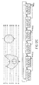
  • Figure 1 is an example of digital images captured by a high speed production scanner without stop and end signals.
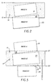
  • Figure 2 is an example of a first captured image frame.
  • Figure 3 is an example of a second captured image frame.
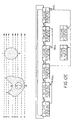
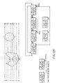
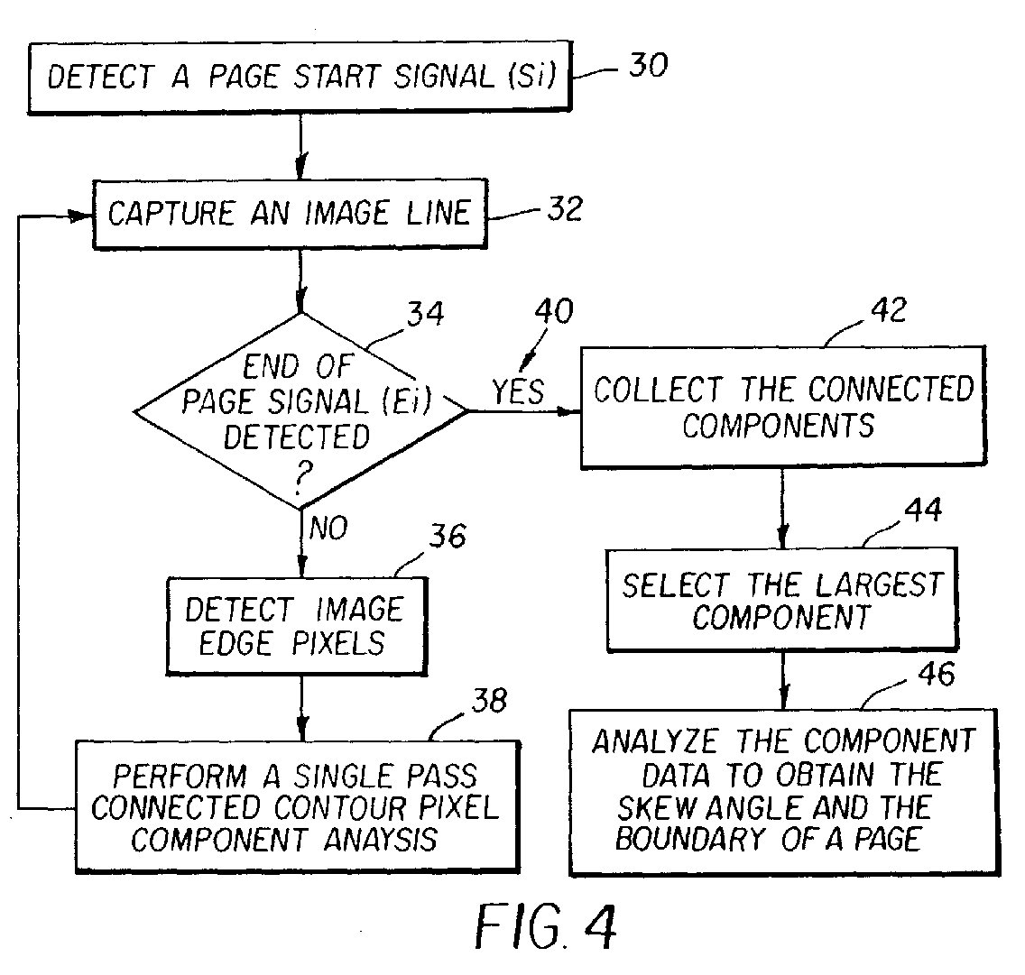
  • Figure 4 is a flow chart outlining the steps of individual image capture and processing in the present invention.
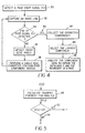
  • Figure 5 is a flow chart showing the steps of detecting image edge pixels.
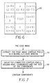
  • Figure 6 shows the position index of 3-by-3 cells for calculating gradient strength.
  • Figure 7 is a flow chart showing the two major processes of performing a single pass connected contour pixel component analysis.
  • Figure 8 shows the steps for extracting contour pixels using a look up table.
  • Figure 9A illustrates the generation of a table integer entry from a 3-by-3 bitmap.
  • Figure 9B is an example of generation of a table integer entry.
  • Figure 9C is an example of generation of template commands using a look up table.
  • Figure 10 a schematic showing four connecting chain codes.
  • Figure 11 is a flow chart illustrating the conversion of template commands into a double link list data chain in tracking and extracting the connected contour components.
  • Figures 12A-E are examples of the step-by-step process for constructing a double link-list data chain for tracking connected contour pixels and for extracting all contour components.
  • Figure 13 is a schematic of the seven extracted connected contour components in Figure 3.
  • Figure 14 is a block diagram for computing skew angle of a contour component.
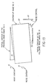
  • Figure 15 is shows the contour of a largest component which is taken as the outline of a page for shape, size, and skew angle analysis.
  • Figure 16 is an example of histogram chart of vertical distance Dy as shown in Figure 15.
  • Figure 17 is an example illustrating the physical intersection points between image scanning lines and the outline of a page.
  • Figure 1 is a graphical example of the resulting image 10 captured by a high speed production scanner if the electronic device which signal start of a scanned page (S1, S2, S3, S4, ...) and end of a scanned page (E1, E2, E3, E4, ...) are off.
  • Each scanned page may have different skew direction.
  • the background black border 12 contains background noises 14 and vertical lines 16 due to dust or dirt blocking the illumination path of light source when a scanning is in progress. Because of high speed paper transport and capture, any two consecutive images 18, 20 can be captured one after the other in very short instance, and the gap between the two captured page images can be very small, and the image content of a current page can contain portions of the preceding and following page images.
  • the S signal i.e. S1, S2, S3, S4
  • the E signal i.e. E1, E2, E3, E4 stops the capture of a page.
  • the S and E signals are to approximately locate each scanned page.
  • Figure 2 shows the region of the captured Image #1 which also contains a small top portion 22 of the following page image (Image #2) and noises.
  • the captured current image 20 as shown in Figure 3 then contains small portions 19 of the preceding page image 18 and small portion 23 the following page image 24 and some unwanted background noises 14.
  • a page start signal (Si) 30 triggers the beginning of a new scan page and starts capturing image line-by-line 32 while a paper document is traveling, until a page ending signal (Ei) is detected 34.
  • every scanline goes through a process of detecting image edge pixels 36, and a single pass connected contour pixel component analysis 38 is immediately followed to group the connected contour pixels.
  • the two operations are repeated on every scanline, until a page end signal is detected 40.
  • the output of the two processes is a connected component data.
  • the connected components data is collected 42.
  • Each component data set contains the coordinates of the contour pixels and its physical size, comprised of component width and component height.
  • the largest component is selected 44 and taken as the page outline component.
  • the skew angle and the boundary of the scanned page are then obtained 46 by analysis of the page outline component data.
  • detection of image edge pixels; a single pass connected outline pixel component analysis; and skew angle and page boundary analysis are presented in the following three sections.
  • the method for detection of image edge pixels is depicted in Figure 5.
  • the detection converts each pixel intensity I(i,j) whose value is between 0 - 255 into a bitmap form.
  • the pixel at the output marked a s"1" is considered as edge pixel and the pixel assigned to "0" is non-edge pixel.
  • a gradient strength for the pixel is calculated 48.
  • Gradient strength for pixel (i,j) is determined by use of the so-called "Sobel” gradient operator on a 3-by-3 window of pixels 50 centered about pixel (i,j) as shown in Figure 6.
  • the Sobel operator relies on computing horizontal and vertical pixel intensity gradients, GX(i,j) and GY(i,j), respectively, and for each pixel position (i,j) forming the gradient strength G(i,j) as an absolute sum of GX(i,j) and GY(i,j).
  • GX(i,j) I(i+1,j-1)+2(i+1,j) + I(i+1,j+1) -I(i-1,j-1) - 2I(i-1,j) - I(i-1,j+1)
  • GY(i,j) I(i-1, j+1) + 2 I(i, j+1) + I(i+1,j+1) -I(i-1,j-1) - 2I(i,j-1) - I(i+1,j-1)
  • G(i,j) GX (i,j) + GY(i,j) where G(i,j) is the gradient strength at pixel (i,j).
  • the value G(i,j) is compared to a constant GT. If G(i,j) is greater than GT 52, the pixel is interpreted as edge pixel and marked as "1". Otherwise, the pixel is interpreted as non-edge pixel 54 and marked as "0". This process is completed for each pixel of a scanline and produces an edge bitmap line.
  • Figure 7 shows the two steps of the processes of the method for extracting the connected contour pixel components in a single pass processing. It reads in the detected edge bitmap in line-by-line fashion.
  • the contour pixels are detected in a moving 3-by-3 local window 56 by means of look up table method and the detected contour pixels are grouped 58 with the connected contour pixels and recorded in a double link list data chain.
  • look up table and the construction of a link list data chain are described below.
  • Figure 8 shows the steps of contour pixel extraction 56.
  • the detection of a contour pixel requires its 3-by-3 neighboring pixels to constitute its connectivity with other contour pixels.
  • the input 60 is a 3-by-3 edge bitmap taken from the previous edge detection.
  • the 3-by-3 bitmap represents the nine cells that lie within a 3-by-3 window at one instant in time as the window is scanned over the edge bitmap lines. Since the value of each cell is either a 0 or a 1 (2 status), the number of bitmap patterns in a 3-by-3 window (9 elements) is 512 (2 power of 9). The 512 patterns are labeled as 0 - 511. In step 62 each number is corresponding to a 3-by-3 bitmap pattern. This information is used as a look up table, step 64, in order to derive template commands, step 66.
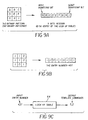
  • FIG. 9A illustrates the specific example as shown in Figure 9A.
  • the bits A through I are arranged in a specific order so as to form a 9-bit integer, the 9-bit integer range in value between 0 and 511.
  • the specific bit pattern selected for the Figure 9B example results in the integer 437 being formed.
  • This integer is then used as an entry number to address the look-up-table as shown in Figure 9C, to output the associated template commands, in this case template commands 5, 2.
  • Table 1 illustrates the relationship between a particular 3-by-3 bitmap and its associated entry number. The entry number being generated according to the procedure previously illustrated in Figure 9C. Table 1 also shows the template commands that are outputted from the look-up-table when the corresponding entry number is applied as an address to the look-up table 64.
  • the template commands, step 66 encode the relationship of the center cell and its neighboring cells in a 3-by-3 bitmap. This template commands are ranged from 0 to 6, and are defined in Table 2.
  • a border transition cell has four possible orientations (0 degree, 45 degree, 90 degree and 135 degree) connecting to its four adjacent pixels in a 3-by-3 bitmap as shown in Figure 10.
  • the four connecting orientations are encoded as commands 0, 1, 2, 3, respectively. All possible local maximum 3-by-3 patterns are shown in Table 3.
  • a local maximum cell for outer contour and for inner contour are encoded as command 4 and 5, which initiates a start of tracking two border pixel strings, respectively. All possible local minimum 3-by-3 patterns are shown in Table 4.
  • a local minimum cell is encoded as command 6 which merges and removes two incoming border pixel strings.
  • a non-border cell is assigned no command. No action is taken when a 3-by-3 window is in a flat region of the edge bitmap.
  • Figure 11 is a block diagram of grouping and recording the connected contour pixels by reading and executing the string of template commands which are generated in an image raster scan fashion.
  • the output of the process is a collection of contour pixel components.
  • Each component data set contains the (x, y) coordinates of contour pixels and its size (width and height).
  • the recording and grouping of the contour pixel components starts with a command which indicates a contour pixel.
  • the command is tested 70 to determine if it is a local maximum (max_point) or not. If it is, two new nodes (Li, Ri), along with two associated border coordinate lists in the link list data string.
  • the two new nodes are assigned to the same identification 72, that is, the left hand sided identification L_ID is set to equal to the right hand sided R_ID.
  • the next template command is read, or the new 3-by-3 bitmap is read for new set of commands, to continue for a next contour pixel. If a command does not indicate a max_point, the command is tested as it is a local minimum (min _point) 74, if it is not, then it is a contour transition pixel whose (x, y) coordinate is saved 76 and the next command is read to extract next contour pixel. If it is a local minimum, the identifications of the two merging contour strings, L_ID and R_ID, are tested 78 if they are the same.
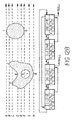
  • FIG. 12A, 12B, 12C, 12D and 12E An example of a link list construction for recording contour pixels is depicted in Figure 12A, 12B, 12C, 12D and 12E.
  • a scanning of the bitmap image from left to right detects a local maximum at 1 in scanline A.
  • the bounding coordinates of the border strings are recorded as (X1, Y1) and (X2, Y2).
  • Next local maximum 2 is detected at scanline B, two additional nodes (L2, R2) are formed to the right of L1 and R1.
  • another local maximum 3 is detected at scanline C, two additional nodes (L3, R3) are formed in between the nodes (L1, R1) and the nodes (L2, R2).
  • a local minimum 4 is detected and signals the merge of the two border chains, R2 and L2.
  • the two nodes, R3 and L2 are removed from the link list loop by resetting the forward'pointer of L3 pointing to R2 pointing to L3.
  • the nodes (L2, R2) and (L3, R3) are part of the same contour and their identifications, L2_ID, R2_ID, L3_ID and R3_ID, are set to the same identification number. In this case, the number I is 6.
  • a new local maximum is detected and two nodes (L5, R5) is inserted in the between the L3 and the R2.
  • Figure 13 displays the extracted contour components for the image 20 in Figure 3 obtained by the processes described in the previous section.
  • the largest component which is labeled as 20 is located in the center of the frame is identified as the outline of the page of interest.
  • the component data which is stored in term of a string (x, y) coordinates along the trace of contour, is taken for analysis to obtain skew angle and the boundary of the scanned page.
  • the skew angle is estimated based on the coordinates of the contour points corresponding to the top border of the page as shown in Figure 14.
  • the contour points in the top border are taken in every Dx increment in horizontal direction 84.
  • the corresponding vertical distance Dy of every pair of subsampled adjacent points is calculated 86.
  • value must be greater than the
  • the remaining data is used to construct a histogram 88 in which the horizontal axis is labeled as Dy and the vertical is labeled the number of Dy counts as shown in Figure 15.
  • the mode (Dm) of the histogram Dy is defined as the value of Dy with the greatest number of hits.
  • K is a threshold value.
  • the linear correlation coefficient (Corr) is calculated 92 and taken as a measure of confidence level in detecting a skewed straight line. If confidence level is below the specified threshold (Ck), the skew angle is set to zero 94. This indicates the page of interest is either upright or it contains irregular top border.
  • the correlation coefficient (r xy ) is defined by and The value of the correlation coefficient is between zero and one, according to the definition. If the correlation coefficient is close to one, it indicates that these points are collinear, and the linear least square fit is applied to these points.
  • the data reorganization is made by sorting the points based the y-coordinate values and stored in a top-to-bottom order. In every y-coordinates, it corresponds to a list of intersection points marked in x-coordinates as shown in Table 5.
  • the x-coordinates in table are the intersection points between image scanning line (y-coordinate) and the image outline which are illustrated in Figure 17. Note that at the tip comer of a contour the intersection point marked with "o" is duplicated in order to guarantee an even number.
  • the x-y coordinates table is applied to border removal either for gray scale image or for binary image.

Landscapes

  • Engineering & Computer Science (AREA)
  • Computer Vision & Pattern Recognition (AREA)
  • Physics & Mathematics (AREA)
  • General Physics & Mathematics (AREA)
  • Multimedia (AREA)
  • Theoretical Computer Science (AREA)
  • Signal Processing (AREA)
  • Image Processing (AREA)
  • Image Input (AREA)
  • Image Analysis (AREA)
  • Facsimile Scanning Arrangements (AREA)
  • Editing Of Facsimile Originals (AREA)
  • Facsimile Image Signal Circuits (AREA)

Abstract

A method for detection of a skew angle and a border of a document scanned by a production scanner comprise the steps of:
  • (a) detecting a page start signal;
  • (b) capturing an image line;
  • (c) checking for an end of page signal;
  • (d) if an end of page signal is detected go to step (h), if no end of page signal is detected go to step (e);
  • (e) detecting image edge pixels;
  • (f) performing a single pass connected contour pixel component analysis;
  • (g) go to step (b);
  • (h) collecting the connected contour pixel components;
  • (i) selecting a largest component; and
  • (j) analyzing the largest component to obtain the skew angle and border of the document.
  • Figure 00000001

    Description

    This invention relates in general to the field of scanning documents and more particularly to detecting a skew angle of documents on the scanner and reorienting the digitized image.
    When a paper document is scanned by a production scanner, the resulting digital image is often skewed. The causes of a skewed image may be that the document was not fed properly, or that the paper transport mechanism is out of alignment. The skew of a document image produces an unpleasant effect on viewing an image. In addition, it results in additional complexities in optical character recognition, document segmentation, and document analysis. Hence, automatic image skew detection and correction are a desired feature in a document scanning system.
    In a production scanning environment, a stack of documents to be scanned often contain different paper sizes. It is impossible to adaptively adjust the CCD scan width to fit all document sizes. To avoid cutoff of a document, the CCD scanning width is often set to a scan a range wider than the document. This results in an unwanted border, either in black or in white, surrounding the original document in the digital image. To produce a digital version which is identical to the appearance and size of the original document, a border detection and removal function in the system is required.
    Two U.S. Patents No. 5,818,976 Method and Apparatus for Document Skew and Size/Shape Detection, and No. 5,901,253 Image Processing System with Image Cropping and Skew Correction, discuss skew angle detection and image border detection for a scanned document. A disadvantage of both methods is the requirement of a clean, uniform background border in order to estimate a skew angle of a document, and to locate the a document page. In a high speed production scanning environment for example, rotary scanning, the background border often contains portions of both the preceding document and the following document, and appears noisy in gray scale due to dust and dirts. The interference of adjacent document images and noises in the background border make the prior art solutions difficult to implemented practically in a high speed scanning system. Another disadvantage of the prior art techniques in border detection is their limitation in handling non-rectangular documents or photographs.
    The present invention is related to an image processing method which is comprised of automatic document skew angle detection, border detections and border removal for any kind of document shapes in an environment having a noisy background, such as interference of adjacent scanned pages and noises in a high speed production scanner.
    Briefly, according to one aspect of the present invention a method for detection of a skew angle and a border of a document scanned by a production scanner comprise the steps of:
  • (a) detecting a page start signal;
  • (b) capturing an image line;
  • (c) checking for an end of page signal;
  • (d) if the end of page signal is detected go to step (h), if no end of page signal is detected go to step (e);
  • (e) detecting image edge pixels;
  • (f) performing a single pass connected contour pixel component analysis;
  • (g) go to step (b);
  • (h) collecting the connected contour pixel components;
  • (i) selecting a largest component; and
  • (j) analyzing the largest component to obtain the skew angle and border of the document.
  • According to one embodiment of the invention the method generally comprises the steps of capturing a document image by a linear CCD array in raster scan fashion and detecting image edge pixels from the captured gray scale image. The connected image contour pixels are traced and grouped and the largest connected contour pixel component is selected as the outline component of the scanned document page. The selected contour component is analyzed to obtain the skew angle and the boundary of a scanned page.
    The invention and its objects and advantages will become more apparent in the detailed description of the preferred embodiment presented below.
    Figure 1 is an example of digital images captured by a high speed production scanner without stop and end signals.
    Figure 2 is an example of a first captured image frame.
    Figure 3 is an example of a second captured image frame.
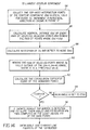
    Figure 4 is a flow chart outlining the steps of individual image capture and processing in the present invention.
    Figure 5 is a flow chart showing the steps of detecting image edge pixels.
    Figure 6 shows the position index of 3-by-3 cells for calculating gradient strength.
    Figure 7 is a flow chart showing the two major processes of performing a single pass connected contour pixel component analysis.
    Figure 8 shows the steps for extracting contour pixels using a look up table.
    Figure 9A illustrates the generation of a table integer entry from a 3-by-3 bitmap.
    Figure 9B is an example of generation of a table integer entry.
    Figure 9C is an example of generation of template commands using a look up table.
    Figure 10 a schematic showing four connecting chain codes.
    Figure 11 is a flow chart illustrating the conversion of template commands into a double link list data chain in tracking and extracting the connected contour components.
    Figures 12A-E are examples of the step-by-step process for constructing a double link-list data chain for tracking connected contour pixels and for extracting all contour components.
    Figure 13 is a schematic of the seven extracted connected contour components in Figure 3.
    Figure 14 is a block diagram for computing skew angle of a contour component.
    Figure 15 is shows the contour of a largest component which is taken as the outline of a page for shape, size, and skew angle analysis.
    Figure 16 is an example of histogram chart of vertical distance Dy as shown in Figure 15.
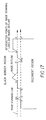
    Figure 17 is an example illustrating the physical intersection points between image scanning lines and the outline of a page.
    Figure 1 is a graphical example of the resulting image 10 captured by a high speed production scanner if the electronic device which signal start of a scanned page (S1, S2, S3, S4, ...) and end of a scanned page (E1, E2, E3, E4, ...) are off. Each scanned page may have different skew direction. The background black border 12 contains background noises 14 and vertical lines 16 due to dust or dirt blocking the illumination path of light source when a scanning is in progress. Because of high speed paper transport and capture, any two consecutive images 18, 20 can be captured one after the other in very short instance, and the gap between the two captured page images can be very small, and the image content of a current page can contain portions of the preceding and following page images.
    In a scan, the S signal (i.e. S1, S2, S3, S4) usually triggers the scanner to start a capture of a new page 18, and the E signal (i.e. E1, E2, E3, E4) stops the capture of a page. The S and E signals are to approximately locate each scanned page. Figure 2 shows the region of the captured Image #1 which also contains a small top portion 22 of the following page image (Image #2) and noises. The captured current image 20 as shown in Figure 3 then contains small portions 19 of the preceding page image 18 and small portion 23 the following page image 24 and some unwanted background noises 14.
    The processing steps of the method in the present invention for detecting skew angle and the boundary of the current page image are shown in Figure 4. A page start signal (Si) 30 triggers the beginning of a new scan page and starts capturing image line-by-line 32 while a paper document is traveling, until a page ending signal (Ei) is detected 34. During the scan, every scanline goes through a process of detecting image edge pixels 36, and a single pass connected contour pixel component analysis 38 is immediately followed to group the connected contour pixels. The two operations are repeated on every scanline, until a page end signal is detected 40. At the end of a page scan, the output of the two processes is a connected component data. The connected components data is collected 42. Each component data set contains the coordinates of the contour pixels and its physical size, comprised of component width and component height. The largest component is selected 44 and taken as the page outline component. The skew angle and the boundary of the scanned page are then obtained 46 by analysis of the page outline component data. The detail descriptions of the three major processes: detection of image edge pixels; a single pass connected outline pixel component analysis; and skew angle and page boundary analysis, are presented in the following three sections.
    Detecting Image Edge Pixels
    The method for detection of image edge pixels is depicted in Figure 5. The detection converts each pixel intensity I(i,j) whose value is between 0 - 255 into a bitmap form. The pixel at the output marked a s"1" is considered as edge pixel and the pixel assigned to "0" is non-edge pixel. First, a gradient strength for the pixel is calculated 48. Gradient strength for pixel (i,j) is determined by use of the so-called "Sobel" gradient operator on a 3-by-3 window of pixels 50 centered about pixel (i,j) as shown in Figure 6. The Sobel operator relies on computing horizontal and vertical pixel intensity gradients, GX(i,j) and GY(i,j), respectively, and for each pixel position (i,j) forming the gradient strength G(i,j) as an absolute sum of GX(i,j) and GY(i,j). The equations of the GX(i,j), GY(i,j) and G(i,j) are defined as: GX(i,j) = I(i+1,j-1)+2(i+1,j) + I(i+1,j+1)    -I(i-1,j-1) - 2I(i-1,j) - I(i-1,j+1) GY(i,j) = I(i-1, j+1) + 2 I(i, j+1) + I(i+1,j+1)    -I(i-1,j-1) - 2I(i,j-1) - I(i+1,j-1) G(i,j) = GX (i,j) + GY(i,j) where G(i,j) is the gradient strength at pixel (i,j). As shown in Figure 5, the value G(i,j) is compared to a constant GT. If G(i,j) is greater than GT 52, the pixel is interpreted as edge pixel and marked as "1". Otherwise, the pixel is interpreted as non-edge pixel 54 and marked as "0". This process is completed for each pixel of a scanline and produces an edge bitmap line.
    A Single Pass Connected Contour Pixel Component Analysis
    Prior techniques to extract the connected outline pixel components can be found in, "Some Experiments in Imaging Vectorization", by J. Jimenez and J. L. Navalon, IBM J res. Develop., vol. 26, No 6, pp. 724-734; "Transforming a Two-Level Image into Contour Vector," by J. Ohta in U.S. Patent No. 5,357,602; and "Chain-Link Coding and Segmentation for Raster Scan Devices," by L. T. Cederberg, Computer Vision, Graphics and Image Processing, vol. 10, pp. 224-234. These prior art methods are not suitable for use in high speed production scanning because they are either not a single pass processing or not computationally efficient. The following method describes a fast, single pass outline pixel component analysis suitable to practical use in high speed scanning systems.
    Figure 7 shows the two steps of the processes of the method for extracting the connected contour pixel components in a single pass processing. It reads in the detected edge bitmap in line-by-line fashion. The contour pixels are detected in a moving 3-by-3 local window 56 by means of look up table method and the detected contour pixels are grouped 58 with the connected contour pixels and recorded in a double link list data chain. The details of the use of look up table and the construction of a link list data chain are described below.
    Figure 8 shows the steps of contour pixel extraction 56. The detection of a contour pixel requires its 3-by-3 neighboring pixels to constitute its connectivity with other contour pixels. Hence, the input 60 is a 3-by-3 edge bitmap taken from the previous edge detection. The 3-by-3 bitmap represents the nine cells that lie within a 3-by-3 window at one instant in time as the window is scanned over the edge bitmap lines. Since the value of each cell is either a 0 or a 1 (2 status), the number of bitmap patterns in a 3-by-3 window (9 elements) is 512 (2 power of 9). The 512 patterns are labeled as 0 - 511. In step 62 each number is corresponding to a 3-by-3 bitmap pattern. This information is used as a look up table, step 64, in order to derive template commands, step 66.
    This is illustrated with the specific example as shown in Figure 9A. The bits A through I are arranged in a specific order so as to form a 9-bit integer, the 9-bit integer range in value between 0 and 511. The specific bit pattern selected for the Figure 9B example results in the integer 437 being formed. This integer is then used as an entry number to address the look-up-table as shown in Figure 9C, to output the associated template commands, in this case template commands 5, 2. Table 1 illustrates the relationship between a particular 3-by-3 bitmap and its associated entry number. The entry number being generated according to the procedure previously illustrated in Figure 9C. Table 1 also shows the template commands that are outputted from the look-up-table when the corresponding entry number is applied as an address to the look-up table 64.
    3x3 bitmap pattern Entry number Template command
    000
    000 0 none
    000
    000
    000 1 none
    001
    000
    010 21 4,5
    101
    000
    010 23 4
    111
    101
    110 368 0,1,3,6,3,6
    000
    110
    110 437 5,2
    101
    111
    111 511 none
    111
    The template commands, step 66, encode the relationship of the center cell and its neighboring cells in a 3-by-3 bitmap. This template commands are ranged from 0 to 6, and are defined in Table 2.
    Template Command Command Definition
    0 Add chain code 0
    1 Add chain code 1
    2 Add chain code 2
    3 Add chain code 3
    4 Initiate a new outer maximum contour point
    5 Initiate a new inner maximum contour point
    6 Merge two incoming border pixel chains
    In a 3-by-3 bitmap, the relationship of a center cell with its neighboring cells can be classified into one or combination of the four conditions: border transition, local maximum, local minimum and non-border. A border transition cell has four possible orientations (0 degree, 45 degree, 90 degree and 135 degree) connecting to its four adjacent pixels in a 3-by-3 bitmap as shown in Figure 10. The four connecting orientations are encoded as commands 0, 1, 2, 3, respectively. All possible local maximum 3-by-3 patterns are shown in Table 3.
    000 000
    011 010
    1xx 100
    000 000
    010 010
    1x1 010
    000 000
    011 010
    01x 001
    000 000
    010 011
    110 000
    000 xxx
    010 x11
    011 100
    000 xxx
    011 x1x
    001 101
    A local maximum cell for outer contour and for inner contour are encoded as command 4 and 5, which initiates a start of tracking two border pixel strings, respectively. All possible local minimum 3-by-3 patterns are shown in Table 4.
    xx1 001
    110 010
    000 000
    1 x 010
    1
    010 010
    000 000
    x10 100
    110 010
    000 000
    110 001
    010 110
    000 000
    110 001
    010 11x
    000 xxx
    100 101
    110 x1x
    000 xxx
    A local minimum cell is encoded as command 6 which merges and removes two incoming border pixel strings. A non-border cell is assigned no command. No action is taken when a 3-by-3 window is in a flat region of the edge bitmap.
    Figure 11 is a block diagram of grouping and recording the connected contour pixels by reading and executing the string of template commands which are generated in an image raster scan fashion. The output of the process is a collection of contour pixel components. Each component data set contains the (x, y) coordinates of contour pixels and its size (width and height). The recording and grouping of the contour pixel components starts with a command which indicates a contour pixel. The command is tested 70 to determine if it is a local maximum (max_point) or not. If it is, two new nodes (Li, Ri), along with two associated border coordinate lists in the link list data string. The two new nodes are assigned to the same identification 72, that is, the left hand sided identification L_ID is set to equal to the right hand sided R_ID. After which the next template command is read, or the new 3-by-3 bitmap is read for new set of commands, to continue for a next contour pixel. If a command does not indicate a max_point, the command is tested as it is a local minimum (min _point) 74, if it is not, then it is a contour transition pixel whose (x, y) coordinate is saved 76 and the next command is read to extract next contour pixel. If it is a local minimum, the identifications of the two merging contour strings, L_ID and R_ID, are tested 78 if they are the same. If it is, then a complete contour is found and the coordinates of the border pixels are collected by retracing the link list nodes 80. If it is not, then the L_ID is set equal to L_IR and remove the two nodes from the link list data string 82 and continue the next template command to start with as shown in Figure 12.
    An example of a link list construction for recording contour pixels is depicted in Figure 12A, 12B, 12C, 12D and 12E. A scanning of the bitmap image from left to right detects a local maximum at 1 in scanline A. When detected, two new nodes (L1, R1), and their L_ID and R_ID are set to a number I=2. The bounding coordinates of the border strings are recorded as (X1, Y1) and (X2, Y2). Next local maximum 2 is detected at scanline B, two additional nodes (L2, R2) are formed to the right of L1 and R1. Continuing the scan, another local maximum 3 is detected at scanline C, two additional nodes (L3, R3) are formed in between the nodes (L1, R1) and the nodes (L2, R2). At the scanline D, a local minimum 4 is detected and signals the merge of the two border chains, R2 and L2. As a result the two nodes, R3 and L2, are removed from the link list loop by resetting the forward'pointer of L3 pointing to R2 pointing to L3. It also indicates that the nodes (L2, R2) and (L3, R3) are part of the same contour and their identifications, L2_ID, R2_ID, L3_ID and R3_ID, are set to the same identification number. In this case, the number I is 6. Continuing the scan, at the scanline E, a new local maximum is detected and two nodes (L5, R5) is inserted in the between the L3 and the R2. A local minimum 6 is detected at the scanline F, it signals the merge of the two incoming border chains, L1 and R1. Since the L1_ID is equal to R1_ID (=2), it indicates that a connected contour pixel component is completed and saved, and the nodes L1 and R1 are removed from the link list loop. The scan is resumed and the detection continues until the end of the bitmap as shown in Figure 12C, 12D, and 12E. At the end of the process, three contours are extracted and the coordinates of contour pixels are read out from the recorded link list chains.
    Calculation of Skew Angle and Boundary of a Scanned Page
    Figure 13 displays the extracted contour components for the image 20 in Figure 3 obtained by the processes described in the previous section. There are seven extracted contour components which are labeled 14, 15, 19, 20, 21, 23, 24, and 25 for the purpose of identification of components. These contour components are either outlines of a scanned pages or contours of noise dots. The largest component which is labeled as 20 is located in the center of the frame is identified as the outline of the page of interest. The component data, which is stored in term of a string (x, y) coordinates along the trace of contour, is taken for analysis to obtain skew angle and the boundary of the scanned page.
    The skew angle is estimated based on the coordinates of the contour points corresponding to the top border of the page as shown in Figure 14. The contour points in the top border are taken in every Dx increment in horizontal direction 84. The corresponding vertical distance Dy of every pair of subsampled adjacent points is calculated 86. For every pair of subsampled adjacent points in the top border, the |Dx| value must be greater than the |Dy| value. Therefore, the pairs of points which shows |Dx| <|Dy| are removed from the recorded data set because they do not belong to the top border. The remaining data is used to construct a histogram 88 in which the horizontal axis is labeled as Dy and the vertical is labeled the number of Dy counts as shown in Figure 15. The mode (Dm) of the histogram Dy is defined as the value of Dy with the greatest number of hits. To minimize the data points which are associated with the boundary noises of a page, those data points, which Dy values fall outside the range of Dm-K and Dm+K 90 as shown in Figure 16, are also deleted, where K is a threshold value. After the process of data cleanup, the remaining data points is evaluated for linearity in the (x, y) domain. The linear correlation coefficient (Corr) is calculated 92 and taken as a measure of confidence level in detecting a skewed straight line. If confidence level is below the specified threshold (Ck), the skew angle is set to zero 94. This indicates the page of interest is either upright or it contains irregular top border. On the other hand, if confidence level is greater than the specified threshold, then it concludes that a slant, straight top border is detected and the equation of the straight line is computed by the least square fit of the data points 96. The skew angle is read from the slope of the fitted straight line, which is arctangent (slope).
    The correlation coefficient is determined as follows. Assume the coordinates of the point are (xi, yi), where I=1, ..., N and N is the number of the remaining data points. The correlation (rxy) is defined by rxy = Sxy/(SxSy).
    The correlation coefficient (rxy) is defined by
    Figure 00140001
    and
    Figure 00140002
    The value of the correlation coefficient is between zero and one, according to the definition. If the correlation coefficient is close to one, it indicates that these points are collinear, and the linear least square fit is applied to these points. The rotating angle S is read from the slope (S = b) of the fitted straight line, y = a + bx , where
    Figure 00150001
    The rotating angle is taken as the skew angle of the scanned documents.
    The value of the coefficient is between zero and one, according to the definition. If the correlation is close to one, it indicates that these data points has perfect linear relationship and the points can be fitted into a straight line, y = a + b x, where the angle which is the skew angel of a scanned page is calculated as the arctangent (b).
    Since the coordinates (x, y) of contour points of a component are sequentially recorded along trace of a contour it requires to reorganize the contour points so that the black border removal can be made in line-by-line order. The data reorganization is made by sorting the points based the y-coordinate values and stored in a top-to-bottom order. In every y-coordinates, it corresponds to a list of intersection points marked in x-coordinates as shown in Table 5.
    Figure 00160001
    The x-coordinates in table are the intersection points between image scanning line (y-coordinate) and the image outline which are illustrated in Figure 17. Note that at the tip comer of a contour the intersection point marked with "o" is duplicated in order to guarantee an even number. The x-y coordinates table is applied to border removal either for gray scale image or for binary image.
    Claims (4)

    1. A method for detection of a skew angle and a border of a document scanned by a production scanner comprising the steps of:
      (a) detecting a page start signal;
      (b) capturing an image line;
      (c) checking for an end of page signal;
      (d) if said end of page signal is detected go to step (h), if no end of page signal is detected go to step (e);
      (e) detecting image edge pixels;
      (f) performing a single pass connected contour pixel component analysis;
      (g) go to step (b);
      (h) collecting said connected contour pixel components;
      (i) selecting a largest component; and
      (j) analyzing said largest component to obtain said skew angle and said border of said document.
    2. A method as in claim 1 wherein said step of detecting image edge pixels is comprised of:
      computing an image intensity gradient in a 3x3 moving window; and
      thresholding said intensity gradient data to extract an edge bitmap of image objects.
    3. A method as in claim 1 wherein said step of performing said single pass connected contour pixel component analysis is comprised of:
      extracting said image edge pixels in a moving 3x3 local window by means of look up table method and a sequence of template commands.
    4. A method as in claim 1 wherein said skew angle is obtained by:
      detecting an orientation of said largest contour component; and
      calculating a skew angle based on said largest contour orientation.
    EP01203137A 2000-08-29 2001-08-17 Method for detection of skew angle and border of document images in a production scanning environment Withdrawn EP1184808A3 (en)

    Applications Claiming Priority (2)

    Application Number Priority Date Filing Date Title
    US65020300A 2000-08-29 2000-08-29
    US650203 2000-08-29

    Publications (2)

    Publication Number Publication Date
    EP1184808A2 true EP1184808A2 (en) 2002-03-06
    EP1184808A3 EP1184808A3 (en) 2003-10-29

    Family

    ID=24607915

    Family Applications (1)

    Application Number Title Priority Date Filing Date
    EP01203137A Withdrawn EP1184808A3 (en) 2000-08-29 2001-08-17 Method for detection of skew angle and border of document images in a production scanning environment

    Country Status (2)

    Country Link
    EP (1) EP1184808A3 (en)
    JP (1) JP2002133424A (en)

    Cited By (6)

    * Cited by examiner, † Cited by third party
    Publication number Priority date Publication date Assignee Title
    GB2391129A (en) * 2002-07-16 2004-01-28 Hewlett Packard Development Co Image processing method comprising detecting image skew and borders.
    EP1408681A1 (en) * 2002-10-01 2004-04-14 Eastman Kodak Company A method for determining skew angle and location of a document in an over-scanned image
    WO2006010769A1 (en) * 2004-07-27 2006-02-02 Hewlett-Packard Development Company, L.P. Document creation system and related methods
    CN102474573A (en) * 2010-06-11 2012-05-23 松下电器产业株式会社 Image processing apparatus and image processing method
    CN109146908A (en) * 2018-07-25 2019-01-04 安徽师范大学 A kind of bianry image stream quick region identification algorithm
    CN110147765A (en) * 2019-05-21 2019-08-20 新华三信息安全技术有限公司 A kind of image processing method and device

    Families Citing this family (1)

    * Cited by examiner, † Cited by third party
    Publication number Priority date Publication date Assignee Title
    JP4238749B2 (en) * 2004-03-10 2009-03-18 カシオ計算機株式会社 Image processing apparatus, image projection apparatus, image processing method, and program

    Family Cites Families (3)

    * Cited by examiner, † Cited by third party
    Publication number Priority date Publication date Assignee Title
    JP3338537B2 (en) * 1993-12-27 2002-10-28 株式会社リコー Image tilt detector
    JPH10208066A (en) * 1997-01-28 1998-08-07 Matsushita Electric Works Ltd Method for extracting edge line of check object and appearance check method using this method
    US6310984B2 (en) * 1998-04-09 2001-10-30 Hewlett-Packard Company Image processing system with image cropping and skew correction

    Cited By (12)

    * Cited by examiner, † Cited by third party
    Publication number Priority date Publication date Assignee Title
    GB2391129A (en) * 2002-07-16 2004-01-28 Hewlett Packard Development Co Image processing method comprising detecting image skew and borders.
    US7068855B2 (en) 2002-07-16 2006-06-27 Hewlett-Packard Development Company, L.P. System and method for manipulating a skewed digital image
    EP1408681A1 (en) * 2002-10-01 2004-04-14 Eastman Kodak Company A method for determining skew angle and location of a document in an over-scanned image
    US7027666B2 (en) 2002-10-01 2006-04-11 Eastman Kodak Company Method for determining skew angle and location of a document in an over-scanned image
    WO2006010769A1 (en) * 2004-07-27 2006-02-02 Hewlett-Packard Development Company, L.P. Document creation system and related methods
    US7262781B2 (en) 2004-07-27 2007-08-28 Hewlett-Packard Development Company, L.P. Document creation system and related methods
    CN102474573A (en) * 2010-06-11 2012-05-23 松下电器产业株式会社 Image processing apparatus and image processing method
    EP2582127A4 (en) * 2010-06-11 2014-07-23 IMAGE PROCESSING APPARATUS AND IMAGE PROCESSING METHOD
    US9088715B2 (en) 2010-06-11 2015-07-21 Panasonic Intellectual Property Corporation Of America Image processing apparatus and image processing method for image correction
    CN102474573B (en) * 2010-06-11 2016-03-16 松下电器(美国)知识产权公司 Image processing apparatus and image processing method
    CN109146908A (en) * 2018-07-25 2019-01-04 安徽师范大学 A kind of bianry image stream quick region identification algorithm
    CN110147765A (en) * 2019-05-21 2019-08-20 新华三信息安全技术有限公司 A kind of image processing method and device

    Also Published As

    Publication number Publication date
    JP2002133424A (en) 2002-05-10
    EP1184808A3 (en) 2003-10-29

    Similar Documents

    Publication Publication Date Title
    EP1014677B1 (en) An artifact removal technique for skew corrected images
    US7636483B2 (en) Code type determining method and code boundary detecting method
    US6160913A (en) Method and apparatus for digital halftone dots detection and removal in business documents
    JP2002133426A (en) Ruled line extraction device for extracting ruled lines from multi-valued images
    JP2007028362A (en) Apparatus and method for processing image data in which background image and target image are mixed
    US6317223B1 (en) Image processing system for reducing vertically disposed patterns on images produced by scanning
    US6687421B1 (en) Skew detection of text in a noisy digitized image
    EP3125159A1 (en) Optical character recognition localization tool
    EP1184808A2 (en) Method for detection of skew angle and border of document images in a production scanning environment
    JP5870745B2 (en) Image processing apparatus, binarization threshold value calculation method, and computer program
    JP4132766B2 (en) Image processing apparatus and method
    JP2871590B2 (en) Image extraction method
    JP2002150213A (en) Barcode reader
    JP5127687B2 (en) Bar code reading apparatus, bar code reading program, and bar code reading method
    JPH11288453A (en) Method and system for detecting skew angle and black boundary line of original image in scan environment for reproduction
    JP4439054B2 (en) Character recognition device and character frame line detection method
    JPH06150059A (en) Image area separator
    JP2795860B2 (en) Character recognition device
    JP2002015283A (en) Separated character string integration method and apparatus
    JP2853140B2 (en) Image area identification device
    JPH06282684A (en) Character recognizing device
    JP3341097B2 (en) Optical character reader
    JPH06139343A (en) Image processing device
    JP2670074B2 (en) Vehicle number recognition device
    JP2001273506A (en) Image data binarization method and apparatus

    Legal Events

    Date Code Title Description
    PUAI Public reference made under article 153(3) epc to a published international application that has entered the european phase

    Free format text: ORIGINAL CODE: 0009012

    AK Designated contracting states

    Kind code of ref document: A2

    Designated state(s): AT BE CH CY DE DK ES FI FR GB GR IE IT LI LU MC NL PT SE TR

    AX Request for extension of the european patent

    Free format text: AL;LT;LV;MK;RO;SI

    PUAL Search report despatched

    Free format text: ORIGINAL CODE: 0009013

    RIC1 Information provided on ipc code assigned before grant

    Ipc: 7H 04N 1/387 B

    Ipc: 7G 06T 7/00 A

    AK Designated contracting states

    Kind code of ref document: A3

    Designated state(s): AT BE CH CY DE DK ES FI FR GB GR IE IT LI LU MC NL PT SE TR

    AX Request for extension of the european patent

    Extension state: AL LT LV MK RO SI

    AKX Designation fees paid
    REG Reference to a national code

    Ref country code: DE

    Ref legal event code: 8566

    STAA Information on the status of an ep patent application or granted ep patent

    Free format text: STATUS: THE APPLICATION IS DEEMED TO BE WITHDRAWN

    18D Application deemed to be withdrawn

    Effective date: 20040430