EP1172980A1 - Dispositif pour la classification de signaux complexes contenant une modulation numérique linéaire - Google Patents
Dispositif pour la classification de signaux complexes contenant une modulation numérique linéaire Download PDFInfo
- Publication number
- EP1172980A1 EP1172980A1 EP01401730A EP01401730A EP1172980A1 EP 1172980 A1 EP1172980 A1 EP 1172980A1 EP 01401730 A EP01401730 A EP 01401730A EP 01401730 A EP01401730 A EP 01401730A EP 1172980 A1 EP1172980 A1 EP 1172980A1
- Authority
- EP
- European Patent Office
- Prior art keywords
- signal
- symbols
- modulation
- estimate
- complex signal
- Prior art date
- Legal status (The legal status is an assumption and is not a legal conclusion. Google has not performed a legal analysis and makes no representation as to the accuracy of the status listed.)
- Granted
Links
- 230000009021 linear effect Effects 0.000 title claims description 27
- 230000006870 function Effects 0.000 claims abstract description 86
- 238000012545 processing Methods 0.000 claims abstract description 30
- 238000004364 calculation method Methods 0.000 claims abstract description 17
- 230000033764 rhythmic process Effects 0.000 claims abstract description 14
- 238000004458 analytical method Methods 0.000 claims abstract description 8
- 230000015654 memory Effects 0.000 claims abstract description 4
- 239000011159 matrix material Substances 0.000 claims description 40
- 238000001914 filtration Methods 0.000 claims description 31
- 238000001228 spectrum Methods 0.000 claims description 23
- 238000005070 sampling Methods 0.000 claims description 13
- 230000004044 response Effects 0.000 claims description 9
- 238000013519 translation Methods 0.000 claims description 9
- 230000002441 reversible effect Effects 0.000 claims description 5
- 230000002123 temporal effect Effects 0.000 claims description 4
- 230000014509 gene expression Effects 0.000 description 44
- 238000011282 treatment Methods 0.000 description 19
- 239000013598 vector Substances 0.000 description 17
- 230000000875 corresponding effect Effects 0.000 description 15
- 238000000034 method Methods 0.000 description 13
- 238000012546 transfer Methods 0.000 description 8
- 238000009826 distribution Methods 0.000 description 7
- 238000004422 calculation algorithm Methods 0.000 description 5
- 238000006243 chemical reaction Methods 0.000 description 4
- 230000003247 decreasing effect Effects 0.000 description 4
- 239000006185 dispersion Substances 0.000 description 4
- 230000003595 spectral effect Effects 0.000 description 4
- 240000008042 Zea mays Species 0.000 description 3
- 230000002596 correlated effect Effects 0.000 description 3
- 230000008449 language Effects 0.000 description 3
- 230000000670 limiting effect Effects 0.000 description 3
- 230000008569 process Effects 0.000 description 3
- 230000009466 transformation Effects 0.000 description 3
- 230000007704 transition Effects 0.000 description 3
- 230000008859 change Effects 0.000 description 2
- 238000004891 communication Methods 0.000 description 2
- 230000006854 communication Effects 0.000 description 2
- 238000010586 diagram Methods 0.000 description 2
- 230000000694 effects Effects 0.000 description 2
- 229940082150 encore Drugs 0.000 description 2
- 230000010363 phase shift Effects 0.000 description 2
- 238000004088 simulation Methods 0.000 description 2
- 230000001502 supplementing effect Effects 0.000 description 2
- 238000010200 validation analysis Methods 0.000 description 2
- HCUOEKSZWPGJIM-YBRHCDHNSA-N (e,2e)-2-hydroxyimino-6-methoxy-4-methyl-5-nitrohex-3-enamide Chemical compound COCC([N+]([O-])=O)\C(C)=C\C(=N/O)\C(N)=O HCUOEKSZWPGJIM-YBRHCDHNSA-N 0.000 description 1
- 241000251184 Rajiformes Species 0.000 description 1
- 229920000297 Rayon Polymers 0.000 description 1
- 238000005311 autocorrelation function Methods 0.000 description 1
- 239000000470 constituent Substances 0.000 description 1
- 238000010276 construction Methods 0.000 description 1
- 230000003111 delayed effect Effects 0.000 description 1
- 238000001514 detection method Methods 0.000 description 1
- 235000021183 entrée Nutrition 0.000 description 1
- 238000011156 evaluation Methods 0.000 description 1
- 229940050561 matrix product Drugs 0.000 description 1
- 238000005259 measurement Methods 0.000 description 1
- 238000012986 modification Methods 0.000 description 1
- 230000004048 modification Effects 0.000 description 1
- 239000002964 rayon Substances 0.000 description 1
- 230000001603 reducing effect Effects 0.000 description 1
- 230000011664 signaling Effects 0.000 description 1
- 241000894007 species Species 0.000 description 1
- 230000001360 synchronised effect Effects 0.000 description 1
- 238000012360 testing method Methods 0.000 description 1
- 230000017105 transposition Effects 0.000 description 1
Images






Classifications
-
- H—ELECTRICITY
- H04—ELECTRIC COMMUNICATION TECHNIQUE
- H04L—TRANSMISSION OF DIGITAL INFORMATION, e.g. TELEGRAPHIC COMMUNICATION
- H04L27/00—Modulated-carrier systems
- H04L27/0012—Modulated-carrier systems arrangements for identifying the type of modulation
Definitions
- the invention relates to the analysis of electromagnetic signals a priori unknown.
- the techniques currently available for the analysis of unknown signals are to search the received signal invariant attributes, by frequency translation or level, in particular. They can involve a Fourier transformation, or a type transformation "wavelets", or a transformation of WIGNER-VILLE, for example.
- the Applicant has posed the problem of obtaining means which help to find the message contained in a signal, or even allow to find this message completely, when know nothing about the exact modulation and the alphabet of symbols used on the program, when, for example, the modulation is digital.
- the processing means comprise means for determining an estimate of the rhythm (1 / T) of the modulation, and projection means, arranged to calculate the components (z p (k)) of the complex signal in a base of functions ( ⁇ i (t)), which is parameterized according to said rhythm (1 / T) of the modulation, and calculation means, operating on these components, in order to determine at least one estimate relating to at least one property of the complex signal, in the group of properties comprising the elementary pulse form (g (t)) of the complex signal, the sequence of symbols (a (k)) of the complex signal and the carrier f 0 used.
- the processing means are arranged to determine an approximate estimate f a of the carrier frequency f 0 of the complex signal, as well as to demodulate this complex signal by this estimate f a .
- the projection means are then arranged to operate on the complex signal (z (t)) after its demodulation by this approximate estimate, while said base of functions is of low frequency, substantially like the spectrum of the complex signal which, after demodulation, is also low frequency.
- the means of calculation include means of matrix calculation on said components.
- the symbol "i", used as an index or as a summation variable is used several times, with different meanings; in fact, the large number of relationships invoked does not allow a different letter to be used systematically each time, and the context in principle removes any ambiguity.
- the sets of values taken by the variables i, k, t, ... are not generally explained, except when necessary. These sets are deduced from the context by taking all the possible values over the entire duration of the analyzed signal.
- the expressions of the minimum and maximum values as a function of the unknowns of the models are of no practical interest in the algorithm.
- estimate and estimate refer to the evaluation of a unknown quantity, without any a priori on the precision of this assessment.
- the invention relates to the analysis of communication signals.
- we start from a received communication signal we are trying to determine the raw information content (i.e. independently of any encryption).
- the signal received has been recorded, and that it is analyzed in delayed time.
- the elementary modulation function (i.e. applied for each symbol) is for example a form of pulse in "raised cosine root" (Fig. 2A).
- a form wave is described for example in the aforementioned work of Proakis, page 536.
- the modulation functions encountered in practice have, as in the example above, lengths greater than T. It follows that the different signals a (k) g (t-kT) (or symbols) emitted successively every T seconds are superimposed partially (Fig. 2B). According to the result of this overlay (Fig. 2C), it is clear that this phenomenon largely contributes to making it difficult to analyze the type of modulation.
- symbols used are chosen in a alphabet or constellation of symbols (example in Figure 2D), also expressed in complex notation.
- the Applicant has posed the problem of determining which is the type of modulation used in a received message, to then determine the parameters used for this modulation, up to the state (or value) of the symbol sequence actually transmitted.
- the symbols contained in the starting signal are drawn of an "alphabet" of a priori unknown symbols, with a basic modulation (the modulation applied to each symbol) which is also unknown.
- the Applicant first observed that, the starting signal being of finite duration, the number of symbols it contains is also finished. The Applicant then thought that after assuming that this starting signal checks the linear digital modulation model it has to exist a means - at least - to find the sequence of symbols, looking at the number of degrees of freedom (or parameters) which are necessary to obtain a representation the starting signal (after approximate demodulation in the example described).
- the Applicant has sought such a means. In doing so, she first focused on how to represent the start signal (preferably after a first demodulation). As will be seen below, she found “basics functions "which allow, by" projection ", to represent most of the signals that can be encountered in practical, with minimal loss of information, negligible in this case.
- the "support" of a function f (x) can be defined as the set of values of the variable x for which the function f (x) is different from zero.
- time functions representing a signal of finite duration.
- the signal z (t) has a bounded support; in the same way, the modulated elementary modulation function g m (t) has a bounded support, which one can call "temporal length" of the elementary modulation.
- the support of the function h m (t) that is to say the length of the time interval over which h m (t) is not zero, is at most equal to the temporal length of the modulation elementary. This is understandable, since the elementary modulation must be able to decompose according to the function h m (t).
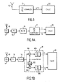
- Figure 1 illustrates the signaling principle complex (100).
- the actual signal received, as from a antenna 10 is defined by the expression E1.
- E1 For treatments, it is subjected to complex filtering 17, the transfer function is adapted to the signal spectrum as we will see it below.
- This filtering provides a computer 20 a complex signal z (t) having a "phase” component I and a "quadrature” component Q.
- this complex signal can be represented as the numbers complex.
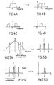
- a complex filter centered on a frequency f 1 can be defined by its impulse response, which corresponds to the relation E2: we start from the impulse response p (t) of a conventional real low-pass filter (Fig. 4A), that we multiply by the expression E3, hence the spectrum shifted from Figure 4B.
- the word “real” here means, as in the following, "with real values", as opposed to complex values.
- FIG. 1A provision is made, after the reception amplifier 11, one or more stages 13 at frequency intermediate (FI), followed by a conversion stage 15 in baseband, then complex filtering 17. Conversion analog digital is usually done either at the input of the stage 15, either inside of it or at its exit (with a lower sampling rate in this last case).
- a stage 18 is provided, with two mixer channels 181 and 182, receiving directly or in quadrature (stage 180) a signal cos 2 ⁇ f 0 t; the mixers are followed by filters 183 and 185, which give the outputs I and Q, respectively.
- Analog to digital conversion is generally done before or after stage 18.
- Stage 200 consists of an estimate of the 1 / T rhythm of the unknown modulation which is presumed to exist in the signal received. We will now describe one of the techniques that can be used for this purpose.
- the rhythm sought corresponds, in the spectrum of this signal x (t), at a frequency line (1 / T). For the rest of the treatments, it is useful to estimate the position of this line, as precisely as possible.
- the spectrum X (f) of the signal x (t) is calculated at 202.
- FFT Interlaced fast Fourier
- each value of X (f) obtained at a frequency f is normalized by the average of the values X (f) obtained for frequencies located in a window of width 2. ⁇ f i , centered around f.
- This processing constitutes a sort of non-linear filtering of the FFT output which aims to bring out the lines contained in this spectrum ( Figure 5B).
- the width 2 ⁇ f i fixes the degree of filtering obtained. Here, it has been fixed by simulation at 20 times the inverse of the total duration of the analyzed signal.
- this signal is thresholded so as to select the lines it contains, and, in 205, the lines at frequencies negative are ignored (Fig. 5C).
- the value 1 / T sought is then estimated in step 206 by an interpolation which can consist in adjusting a curve, of the type polynomial, for example, which goes through the vertices of these different sub-lines and taking the most out of this curve.
- an approximate estimate f a of the carrier frequency f 0 is determined (stage 300).
- the approximate estimate is useful, insofar as it will be used to carry out a first demodulation, which makes it possible to work then at low frequency: the base of functions will be defined in low frequency, and the matrix calculations will be carried out on samples also available at low frequency.
- This technique is based on the fact that, if ⁇ is small before T, the difference between the phase of the signal z (t) at time t and the phase at time (tz) depends only on ⁇ and f 0 .
- ⁇ can be chosen equal to the sampling step (case of Figure 6), or calculated by taking a small fraction of T.
- demodulation consists of a complex multiplication of the signal z (t) by an expression similar to E3, where f 1 is replaced by -f a .
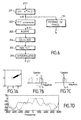
- the initial spectrum (Fig. 7B) of the complex signal comes to center approximately on the zero frequency (Fig. 7C).
- the residual off-center of the spectrum corresponds to a small carrier residue ⁇ f 0 equal to f 0 - f a .
- FIG. 7D An example is given in FIG. 7D, where the mixed line represents the spectrum of the signal before demodulation, while the solid line represents the spectrum of the signal after demodulation.
- the index m means "modulated"
- k is from 1 to kx, which is the total number of symbols involved in the analyzed signal.
- E14 is "without apparent carrier”, that is to say that the carrier residue ⁇ f 0 no longer appears there explicitly. Indeed, it is contained in the “modulated” elementary modulation function g m (t) and in the modulated symbols a m (k).
- stage 500 (501-520) consists in estimating the modulated elementary modulation function, that is to say of the function g m (t). We will deduce from this the symbols modulated a m (k) at stage 600 (610-650) (see Figure 3).
- the Applicant proposes to make an approximation, by projecting the signal z (t) on a "base" of functions, chosen in advance.
- This base (in the mathematical sense of the word) is in fact a free family, preferably orthonormal, of functions ( ⁇ 1 (t), ⁇ 2 (t), ..., ⁇ b (t)).
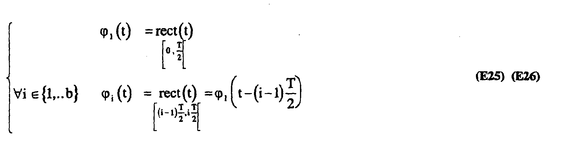
- a base of functions ( ⁇ 1 , ⁇ 2 , ... ⁇ b ) adapted to the rhythm 1 / T as previously estimated, and constructed for example as indicated in expressions E25 and E26.
- rect () denotes the rectangular function over the time interval indicated below.
- the integer q is such that the product qT is substantially equal to the length of the signal analyzed.
- b corresponds to the number of basic functions necessary to cover the entire duration of the signal analyzed.
- the approximation then begins with the calculation of the projection of the signal z (t) in space (also in the mathematical sense of the word) generated by the functions ⁇ i (t).
- This projected signal will then only be defined by projection coefficients, which will be in finite number, less than the number of time samples of the signal z (t).
- the signal z (t) is therefore first of all projected (510, fig. 3) on the basis of functions defined by the relationships E25 and E26. This projection is noted z p (t), where the index p means “projected”.
- the signal is centered on the zero frequency and has, in practical cases, a spectral band of width 1 / T.
- the projection filter is also centered on the zero frequency; on the other hand, it has a band of 2 / T (at 4 dB).
- the prior estimation of the rhythm allows that the projection of the signal on the basis of functions is well synchronized with the modulation rhythm; the estimation of the average instantaneous frequency allows this projection is done on the basis of low frequency functions.
- the Applicant endeavored to find the one which verifies the following property: it is the solution giving symbols modulated to m (k) which, after demodulation, will take a finite number, and the most small possible, of values.
- the projection z p (t) of z (t) can only be modeled from the projection h pm (t) of h m (t).
- the (small) part of the signal that is orthogonal to the projection "base” is lost.
- the function base E25, E26 has been chosen so that the part of the signal lost is sufficiently weak for the signals encountered in practice.
- the signal z (t) is projected on the basis of functions ⁇ i (t).
- this consists, in 510, of filtering the signal z (t) by the impulse response filter ⁇ 1 (-t) (expression E25), then, in 523, of sampling the output of this filter every T / 2 seconds, until the end of the signal z (t).
- the projection z p (t) of the signal z (t) can be written from its projection coefficients z (k) according to the relation E36 (with p for projected).
- the projection h pm (t) of the smallest support function h m (t) is written according to the relation E37, where L is the length of h pm (t), counted in number of periods T In other words, the length of h pm (t) is greater than (L-1) .T and less than or equal to LT
- the first stage of the processing consists in estimating the length L of h pm (t).
- the Applicant has noticed that the lengths of the elementary modulation functions g m (t) encountered in practice are generally less than 10 times T.
- step 525 corresponds to a single-column vector or matrix Z L1 (k) conforming to the expression E41.
- the vectors Z L1 (k) correspond to signal slices z (t) taken between instants kT and (k + L1) T.
- This vector Z L1 (k) contains 2.L1 successive components in r (k), going from (2.k + 1) to (2.k + 2.L1).
- Z L1 (k) largely overlap each other: Z L1 (k + 1) is deduced from Z L1 (k) by suppressing at the top z (2k + 1) and z (2k + 2), by moving the other elements up two boxes, and adding z (2k + 2L1 + 1) and z (2k + 2L1 + 2) at the bottom.
- the construction of these vectors Z L1 (k) from the basic data is therefore done with an interlacing.
- M L1 of dimension 2.L1, defined by the relation E42. It is a kind of covariance matrix of the quantities z (k); however, unlike the usual covariance, the constituent vectors are interlaced; this is why the Applicant proposes to name M L1 the "interlaced covariance matrix".
- the eigenvalues of M L1 are calculated in 529 in a known manner. The analysis of these gives access to the length L of the function h pm (t), because the Applicant has established that the matrix M L1 has L 1 + L - 1 positive eigenvalues nonzero, and L 1 - L + 1 (less than L 1 + L - 1) zero eigenvalues, in fact almost zero because of the noise.
- the length L of the function h pm (t) is given by the rank after sorting of the first zero eigenvalue.
- This matrix M L is another "interlaced covariance matrix", but with an interlacing restricted to L instead of L1.
- the vectors Z L (k) correspond to slices of the signal z p (t) taken between the instants kT and (k + L) T.
- the processing is then as follows.
- the lowest eigenvalue of M L is determined by calculating, for example, as before, all the eigenvalues (which are positive because of the Hermitian symmetry of M L ) and by ranking them in descending order.
- the projection coefficients of h pm (t) are therefore obtained (except for the sign) by taking in order the complex conjugates of the components of this eigenvector, and by changing the sign of these components once in two ( we can work close to the sign).
- steps 535 to 539 are the same than 525 to 529, replacing L1 with L. They can therefore be implemented by the same computing means.
- the signal z p (t) therefore takes its values in a space of dimension L 1 + L-1.
- the matrix M L1 defined above makes it possible, by diagonalization, to estimate the subspace containing these signal slices, from the eigenvectors associated with the nonzero eigenvalues. To simplify the treatment, we can, as described, estimate only the rank L 1 + L-1 of this matrix M L1 (number of eigenvalues which are not very weak or zero). After having deduced L therefrom, it is then possible to re-cut the signal into sections of length LT
- stage 600 is the estimation of the train of modulated symbols c m (k), associated with this estimated function h pm (t).
- each column has qL components.
- the first column is obtained by taking the last q components of h pm (t), and supplementing with zeros.
- each column is deduced from the previous one by a shift of q boxes downwards, by completing at the top with the components of h pm (t) in order, then by zeros, when these components are exhausted.
- the signal z p (t) is then applied in 610 to the inverse filter thus obtained.
- the output corresponds to the symbols c m (k) of the expression E43, in which ⁇ i is the filtering residue and the a m (k) correspond to the symbols sought, modulated by the carrier residue ⁇ f 0 , all these quantities being still unknown at this stage of the algorithm.
- the Applicant has considered imposing the following condition: the symbols a m (k), associated with the filtering residue ( ⁇ i ), must correspond to modulated symbols, which, after demodulation, will take a finite number, and the smallest possible, of values.
- the condition that the Applicant prefers to impose today is: "the train of symbols (a m (k)) is, among the possible solutions giving decorrelated symbols, that for which the alphabet (set of possible values) is of size the smallest”.
- the decorrelation condition of the symbols is given by the relation E70 and relates to the covariance of the symbols.
- the second condition consists in fact in choosing among the solutions making it possible to overcome the first constraint, the train of symbols whose variance of the module of the symbols is the smallest (equation E80).
- the individual elements ( ⁇ i ) of the filtering residue are obtained in 650.
- N 10 as an upper bound, but this value is configurable in the algorithm. Taking an upper bound can only have the effect that the last coefficients ⁇ i with i ⁇ ⁇ n + 1, ..., N ⁇ are zero, if this upper bound N turns out to be greater than n.
- the processing 700 consists in testing all or part of a frequency range [-f 1 , f 1 ], discretized with a sufficiently fine step.
- the probability density d (x, y) of the corresponding symbols is calculated according to the formula E82, or else another quantity with the same properties.
- the criterion used to select the right value consists in choosing the frequency ⁇ f o such that the E85 expression is maximum. We can assimilate the maximization of this criterion to a minimization of the entropy (measure of disorder) of the symbols obtained after demodulation. It would also be possible to replace this criterion with other functions of entropy.
- a demodulation 800 makes it possible to obtain the train of symbols a (k) which corresponds to it.
- This demodulation consists of a complex multiplication of the signal by an expression similar to E3, where f 1 is replaced by - ⁇ f o .
- stage 900 It is still necessary to estimate the possible states of the symbols (stage 900).
- This stage takes into account the fact that the symbols obtained after demodulation correspond to the true symbols, with number of finite states, but corrupted by the noise of power ⁇ 2 , calculated previously, as shown in FIG. 16 which corresponds to an example of result got.
- the different values of the symbols a (k) found are drawn in the complex plane.
- Figure 2D corresponds to the alphabet of symbols a (k) actually emitted for this example.
- the phase rotation between the two figures, as well as the different scales, comes from the fact that, all being unknown at the start, it is only possible to find the train of symbols again to within a complex multiplicative constant.
- the criterion for stopping this treatment (condition "COND" in 907), allowing to know if all possible states have been estimated, maybe that of the expression E86, where ⁇ is a threshold which is fixed in advance (0 ⁇ ⁇ 1).
- the principle used is as follows. It is assumed that the values of the symbols emitted are equally distributed between the different possible values of the alphabet (we have roughly the same number of symbols in each of the modes of FIG. 18, for example).
- the density integrals of the expression E86 are proportional to the numbers of symbols forming these densities.
- n - 1 states e 1 , ..., e n-1 a measure of the average number per state of symbols corresponding to the states e 1 , ..., e n-1 (right member of E86) and in comparing this quantity with the measure of the number of symbols remaining. If this last quantity is too small, it means that there are not enough symbols left to form an additional state.
- These symbols are supposed to be far from states e 1 , ..., e n estimated, because of noise peaks.
- This part of the processing consists, from the train of noisy symbols a (k) and of the possible states of the symbols e 1 , e 2 , ... calculated previously, to estimate, for each noisy symbol a (k), the state e (k) intentionally issued.
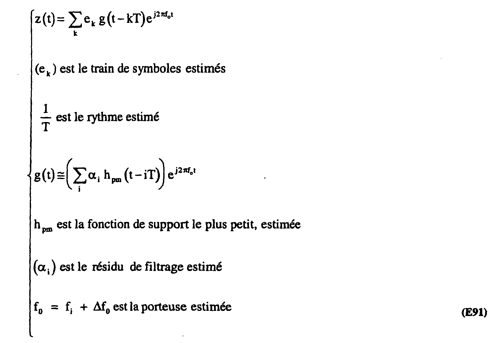
- the preceding treatments made it possible to estimate the elements recalled in E91.
- the quantity defined by the expression E92 is now calculated, and this quantity is compared to a threshold corresponding to the admissible power of the noise.
- This admissible power corresponds to the noise power ⁇ 2 calculated in the "calculation of h pm (520) part, multiplied by the ratio between the sampling frequency of the starting signal and the rhythm of the projection (q / T), and weighted by a coefficient ⁇ (0 ⁇ ⁇ 1) to take account of imperfections in the previous estimates of the parameters
- the value of ⁇ is fixed by simulation.
- the difference between the signal received and the estimated linear digital modulation must be a signal corresponding to noise, of low power; through against, when the signal received is not a modulation linear numeric, said difference is no longer a low power signal that can be seen as noise.
- the treatments described can be implemented on a PC Pentium type workstation, with software tools specific to computational processing, such as software MATLAB.
- Programs prepared under MATLAB can be used as is, or better transformed into a language of faster programming at runtime, like C language MATLAB to C language conversion utilities are available for example from software distributors MATLAB.
- the base of "rectangular" functions described above is not not limiting. Other sets of functions can be used that meet the condition of defining a base, not necessarily orthonormal, provided that the correlation induced on the projection coefficients.
- This treatment remains applicable with any base of functions for which the projection can be interpreted as filtering followed by sampling all T / 2 (that is to say 2 points per symbol).
- the new measures z (k) (signal projection coefficients) are modeled in the form of the relations E50.
- the matrix M L1 can be formed and treated as above. It is given by the expression E52. This matrix M L1 has for the same reasons as previously pL 1 eigenvalues of which L + L1 - 1 are non-zero. The distribution of the eigenvalues is that of figure 13. The break of the diagram allows here also to estimate the length L (in number of T) of the function h pm (t).
- the Applicant plans to calculate and use the eigenvectors V i , from V L1 + L to V q.L1 , associated with the zero eigenvalues of the matrix M L1 .
- the qL 1 components of such a vector (of index i) are noted as indicated in E55, with i ⁇ ⁇ L 1 + L, ...., pL 1 ⁇ .
- matrices P i defined in E56. These are rectangular matrices of dimension qL * q (L 1 + L) -1, formed in the same way as the matrix H allowing the inverse filter to be generated at h pm (t). Each column of such a matrix has qL components. The first column is obtained by taking the last q components of the vector V i considered, and by supplementing with zeros. For the rest, each column is deduced from the previous one by a shift of q boxes downwards, by completing at the top with the components of V i in order, then by zeros when these components are exhausted.
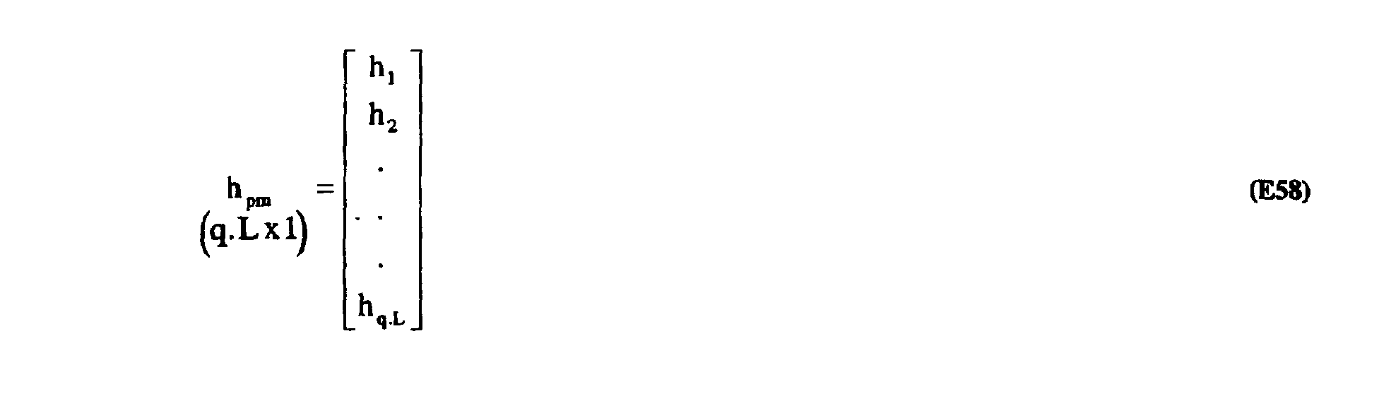
- this matrix has a only zero eigenvalue (excluding noise), and that the vector eigen associated with this eigenvalue obeys the relation E58.
- the power ⁇ 2 of the noise is in this case estimated by taking the average of the almost zero eigenvalues, divided by L1.
- f a the carrier frequency f 0 .
- Different techniques are available for this purpose. We can for example estimate f a by finding the frequency, which after demodulation of the signal by it, minimizes the quadratic band of the signal. If we manage to make the residual difference negligible, then the estimation stage of ⁇ f o and the demodulation which follows it become irrelevant.
- the captured and recorded starting signal is not always comparable to the signal actually transmitted, from which it may differ for various reasons, for example multiple propagation paths. This may result in adjustments to certain stages of treatment.
- Multipaths which can be pictured as echoes, modify the form of the function g (t) and more particularly increase its length. The modification of the form does not change the algorithm since it estimates this form without a priori. On the other hand, it is necessary to increase the upper limits L1 and N of the lengths of h pm and ⁇ i . These parameters which can be configured in the algorithm are to be fixed according to the maximum length of the supposed echoes.
- the invention has been defined essentially with reference to linear digital modulation. It can extend to other types of modulation to which the proposed stages of treatment would agree, at least in part. This is particularly the case for related types of modulation, such as digital frequency modulation with continuous phase, among other codings by frequency hopping (or FSK, for "Frequency Shift Keying").
- related types of modulation such as digital frequency modulation with continuous phase, among other codings by frequency hopping (or FSK, for "Frequency Shift Keying").
- FSK Frequency Shift Keying
Landscapes
- Engineering & Computer Science (AREA)
- Computer Networks & Wireless Communication (AREA)
- Signal Processing (AREA)
- Digital Transmission Methods That Use Modulated Carrier Waves (AREA)
- Radar Systems Or Details Thereof (AREA)
- Amplitude Modulation (AREA)
- Control Of High-Frequency Heating Circuits (AREA)
Abstract
Description
- une mémoire de signal, pour stocker un signal numérique complexe (z(t)), représentatif en amplitude et phase d'un signal capté, sur une durée choisie, et
- des moyens de traitement, agencés pour rechercher dans le signal complexe des propriétés relatives à sa fréquence porteuse et à la modulation de celle-ci, en fonction d'un modèle de modulation, en particulier linéaire.
- la base de fonctions est paramétrée pour présenter au moins deux échantillons par période (T) de la modulation, et plus généralement q échantillons par période (q ∈ N et q ≥ 2);
- elle comprend au moins deux fonctions (ϕ1(t),...,ϕb(t)) se déduisant l'une de l'autre par une translation temporelle de période choisie (T/2 ou plus généralement T/q, q ∈ N et q≥2);
- elle peut être fondée notamment sur des fonctions rectangulaires temporellement adjacentes les unes aux autres, ou encore sur des fonctions du type "cosinus surélevé".
- des moyens définissant un filtre numérique, ayant une réponse impulsionnelle sensiblement égale à l'une desdites fonctions, ce filtre numérique recevant le signal complexe, et
- des moyens d'échantillonnage numérique répété de la sortie de ce filtre à une cadence choisie (2/T;q/T, q ∈ N et q ≥ 2), suivant le type de base choisie.
- la figure 1 illustre schématiquement, sous forme de diagramme-blocs, le principe du passage en signal complexe (100);
- la figure 1A illustre schématiquement un premier mode de réalisation permettant de mettre en oeuvre le principe du passage en signal complexe de la figure 1;
- la figure 1B illustre schématiquement un second mode de réalisation permettant de mettre en oeuvre le principe du passage en signal complexe de la figure 1;
- la figure 2A illustre un exemple de fonction de modulation élémentaire sous la forme d'une impulsion en "racine de cosinus surélevé", en fonction du temps exprimé en périodes T;
- la figure 2B illustre une superposition de signaux a(k)g(t-kT) (ou symboles) émis successivement, en fonction du temps exprimé en périodes T;
- la figure 2C illustre la résultante des signaux de la figure 2B;
- la figure 2D illustre une répartition de symboles (ou constellation) dans le plan complexe, dite "alphabet";
- la figure 3 illustre les principales étapes (ou stades) de traitement du procédé selon l'invention;
- les figures 4A à 4D illustrent respectivement une réponse impulsionnelle d'un filtre passe-bas réel classique, une fonction de transfert du filtre de la figure 4A, un spectre de signal d'entrée, et le spectre du signal complexe du filtre ayant la fonction de transfert de la figure 4B;
- les figures 5A à 5D illustrent respectivement le spectre d'un signal obtenu à partir d'une FFT, un filtrage non linéaire de la sortie de la FFT de la figure 5A, un exemple de traitement des raies de la figure 5B, et un exemple d'estimation de la raie en + 1/T de la figure 5C;
- la figure 6 illustre sous forme d'étape un exemple de traitement permettant d'obtenir la valeur 1/T de la raie isolée de la figure 5D;
- les figures 7A à 7D illustrent respectivement un exemple de signal défini par un nuage de points dans le plan complexe, le spectre du signal complexe de la figure 7A, le spectre du signal complexe de la figure 7B après démodulation, et la densité spectrale du signal de la figure 7A avant et après démodulation;
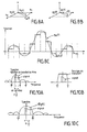
- les figures 8A et 8B illustrent respectivement les projections de hm et du signal dans une base de fonctions choisie;
- la figure 8C illustre une approximation des fonctions gm(t) dans la base de fonctions choisie aux figures 8A et 8B;
- la figure 9 illustre sous forme d'étapes un exemple du déroulement des traitements visant à estimer hm(t);
- les figures 10A à 10C illustrent respectivement le spectre de la fonction de transfert du filtre de réponse impulsionnelle pour un signal centré du type de celui de la figure 7C et pour un premier type de base, le spectre de la fonction de transfert de fonctions ϕ en cosinus surélevés, et le spectre de la fonction de transfert du filtre de réponse impulsionnelle correspondant à la figure 10B;
- la figure 11 illustre l'approximation de hm(t) par sa projection hpm(t) dans la base de fonctions de la figure 10C;
- la figure 12 illustre la répartition des valeurs propres de la matrice ML1, rangées par ordre décroissant de grandeur en abscisse, lorsque la projection correspond à un filtrage suivi d'un échantillonnage à q = 2 points par symboles;
- la figure 13 illustre la répartition des valeurs propres de la matrice ML1, rangées par ordre décroissant de grandeur en abscisse, lorsque la projection correspond à un filtrage suivi d'un échantillonnage à q > 2 points par symboles;
- les figures 14A à 14C illustrent respectivement, en fonction du temps exprimé en périodes T, la fonction hpm(t), le résidu de filtrage, et la fonction élementaire de modulation modulée gpm(t);
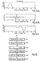
- la figure 15 illustre sous forme d'étapes un exemple du déroulement des traitements visant à estimer les symboles am(k) à partir des trains de symboles possibles;
- la figure 16 illustre un exemple de dispersion du fait du bruit des symboles a(k), dans le plan complexe et pour une plage de fréquence (résidu de fréquence) bien centrée;
- la figure 17 illustre un second exemple de dispersion du fait du bruit des symboles a(k), dans le plan complexe et pour une plage de fréquence mal centrée;
- la figure 18 est une représentation tri-dimensionnelle de la densité de probabilité des symboles a(k) de la figure 16;
- la figure 19 est une représentation tri-dimensionnelle de la densité de probabilité des symboles a(k) de la figure 17;
- la figure 20 illustre sous forme d'étapes un exemple du déroulement des traitements visant à estimer la position des états possibles; et
- la figure 21 illustre sous forme d'étapes un exemple du déroulement des traitements visant à estimer la suite des symboles effectivement émise, à partir du train de symboles bruités a(k) et des états possibles des symboles ei calculés en référence à la figure 20.
- les a(k) (k entier positif) sont les symboles d'information transmis, qui ne peuvent prendre qu'un nombre fini de valeurs possibles, ou états,
- g(t) est la fonction de modulation élémentaire (ou "forme d'impulsion élémentaire"), appliquée à chaque symbole,
- 1/T est le rythme d'émission des symboles, et
- f0 est la fréquence porteuse utilisée.
- la modulation par codage à saut de phase (PSK pour "phase shift keying"),
- la modulation par codage à saut d'amplitude (ASK pour "amplitude shift keying"), et
- la modulation d'amplitude en quadrature (QAM pour "Quadrature Amplitude Modulation").
- passage en signal complexe z(t) (100),
- estimation du rythme 1/T (200),
- estimation "approchée" fa de la fréquence porteuse f0 (300),
- démodulation du signal complexe z(t) par cette fréquence porteuse approchée fa (400),
- estimation de la fonction hpm(t) (500,501,510,520),
- estimation des symboles modulés cm(k) associés à hpm(t) (610),
- estimation du résidu de filtrage αi et des symboles am(k) à partir des symboles cm(k) (650),
- estimation du résidu de porteuse Δf0 (700),
- démodulation des symboles am(k) par le résidu de porteuse (800), afin qu'il ne reste que des symboles a(k),
- estimation des états ou valeurs possibles ei des symboles a(k) à l'aide de l'alphabet (900),
- estimation du train de symboles effectivement émis e(k) en fonction des états possibles (950),
- détermination de l'adéquation du modèle d'une modulation numérique linéaire (990), utilisant les paramètres estimés précédemment (validation ou non de l'hypothèse).
Mais il doit être clair, comme déjà indiqué, que la mise en oeuvre de l'invention peut se faire à partir d'un signal enregistré, ayant déjà subi une partie des traitements, en particulier le passage au signal complexe, auquel cas il est déjà disponible en mémoire 100.
- comme en 201, on prend d'abord le signal x(t) de l'expression E4, puis
- en 311, on calcule la valeur moyenne de la phase de x(t), sur l'ensemble de la durée du signal, et on la divise par 2πτ.
- une fonction de modulation élémentaire modulée gm(t), définie par la relation E12, et
- une suite de symboles modulés am(k), définie par la relation E13.
Dans ces expressions, rect() désigne la fonction rectangulaire sur l'intervalle de temps indiqué en dessous. L'entier q est tel que le produit q.T soit sensiblement égal à la longueur du signal analysé. b correspond au nombre de fonctions de base nécessaire pour couvrir toute la durée du signal analysé.
- parmi les nombreuses solutions possibles de la modélisation, il n'en existe qu'une seule (cm(k),hm(t)) vérifiant la relation E20, où hm est, parmi les fonctions de modulation solutions, celle dont la longueur du support est la plus petite ;
- en outre, cette solution particulière (cm(k),hm(t)) engendre l'ensemble des solutions possibles de la façon suivante: si (am(k),gm(t)) est une autre solution, alors il existe n coefficients (α1, ...αn) permettant de vérifier l'expression E21 donnant gm(t), tandis que les symboles am(k) sont définis récursivement, pour tous les k, par l'expression E23.
- dans un premier temps, on recherche la solution (cm(k),hm(t)) avec la contrainte que hm(t) ait le support le plus petit possible,
- ensuite, à partir des symboles cm(k) correspondant à cette solution hm, et se modélisant selon l'expression E23, on estime la deuxième partie de la fonction gm, à savoir les coefficients (αi), qu'on nomme globalement "résidu de filtrage".
- que la matrice ML a dans ce cas une seule valeur propre λ presque nulle,
- que la grandeur de cette valeur propre permet d'estimer la puissance du bruit σ2 = λ / L, et
- que le vecteur propre associé à cette valeur propre (expression E45) ne dépend que de la fonction hpm(t), solution ayant le support le plus petit.
- les vecteurs ZL1(k) correspondent à un découpage du signal zp(t) en tranches de longueur L1.T, qui se recouvrent;
- ces vecteurs sont définis par les 2.L1 coefficients de projection (z(2k + 1),...,z(2k + 2L1)), qui sont a priori susceptibles de prendre n'importe quelle valeur dans l'espace vectoriel de dimension 2.L1 correspondant;
- cependant, sur chaque tranche ce signal zp(t) devient le signal u(t) conforme à la relation E47, dont les éléments z1(t),...,zL+L1-1(t) sont définis par les relations E48;
- par conséquent, sur chacune de ces tranches, le signal zp(t) est toujours une combinaison linéaire des mêmes (L1+ L - 1) signaux z1(t),...,zL+L1-1(t), combinaison linéaire dont les coefficients sont les symboles cm(k) intervenant dans la tranche considérée et variant donc d'une tranche à l'autre;
- bien que défini au départ à partir de ses 2.L1 coefficients de projection (z(2k + 1),...,z(2k + 2L1)), chaque tranche du signal zp(t) ne prend donc en fait ses valeurs que dans le même sous-espace de fonctions engendré par les L1 + L - 1 signaux définis ci-dessus.
- on sait maintenant que chacune des tranches de longueur L.T du signal zp(t) est susceptible a priori de prendre ses valeurs dans un espace de dimension 2.L ; mais qu'en fait
- sur chacune de ces tranches, le signal zp(t) est toujours une combinaison linéaire des mêmes (2.L-1) signaux s1(t)...SL+L-1(t) de l'équation E48 où l'on remplace L1 par L.
- en 653, on calcule les N racines complexes βi de module inférieur à 1 de ce polynôme Q(Z),
- en 655, on construit les 2N possibilités différentes de N-uplets construites à partir des N racines βi, en remplaçant, ou non, chaque racine βi par son inverse conjugué 1/βi*. Chacun des N-uplets est alors interprété comme les racines d'un filtre,
- en 657, on obtient ainsi 2N filtres possibles dont l'un correspond au résidu de filtrage αi que l'on cherche à calculer,
- puis, en 658, pour chaque possibilité de filtre ainsi obtenue, on estime à partir des symboles cm(k) le train de symboles am(k) qui lui correspond (par filtrage inverse) conformément à la relation E23.
- si βi est une racine de P2 alors 1/βi* est aussi une racine de P2,
- si βi est une racine de P2 alors βi ou bien 1/βi* est une racine du polynôme P qu'on cherche à estimer.
- la figure 14A illustre la fonction hpm(t) ;
- la figure 14B illustre le résidu de filtrage, où se détachent des pics correspondant aux coefficients αi ;
- la figure 14C illustre la fonction élementaire de modulation modulée gpm(t) ; et
- la figure 17 illustre les symboles am(k) en sortie du traitement, qui correspondent aux symboles recherchés, mais demeurant modulés par le résidu de porteuse Δfo.
- on estime le premier état possible e1 comme la position en (x,y) du maximum de la densité de probabilité d(x,y) des symboles bruités,
- à partir de cette densité, on construit la fonction d2(x,y) correspondant à d(x,y), mais dont on force la valeur à zéro pour tous les points se trouvant dans un rayon de 3σ (par exemple) autour de e1,
- on estime alors le deuxième état possible e2 en prenant la position en (x,y) où la fonction d2 est maximale,
- on continue ainsi le traitement jusqu'à ce que tous les états possibles soient traités.
- si l'on prend par exemple pour ϕ1 une fonction en cosinus surélevé de largeur spectrale 2/T, (les autres fonctions ϕi en étant déduites comme précédemment), les spectres sont alors ceux de la figure 10B. L'homme du métier comprend que, du fait de la forme rectangulaire du spectre de ϕ1, on perd encore moins de signal par la projection ;
- on peut aussi prendre la base de fonctions des relations E34 et E35. Ceci revient (Figure 10C) à filtrer le signal par la nouvelle fonction ϕ1(t) et à échantillonner tous les T/q (échantillonnage à q points par symboles, avec q > 2). Comme le montre la figure 11, comparativement à la figure 8C, l'approximation de hm(t) par sa projection hpm(t) dans cette « base » est meilleure.



























Claims (21)
- Dispositif d'aide à l'analyse de signaux contenant une modulation numérique par des symboles, ce dispositif comprenant:caractérisé en ce que les moyens de traitement comprennent:une mémoire de signal (100), pour stocker un signal numérique complexe (z(t)), représentatif en amplitude et phase d'un signal capté, sur une durée choisie, etdes moyens de traitement (200-900), agencés pour rechercher dans le signal complexe des propriétés relatives à sa fréquence porteuse et à la modulation de celle-ci, en particulier en fonction d'un modèle de modulation choisi,des moyens (200) pour déterminer une estimée du rythme (1/T) de la modulation,des moyens de projection (510), agencés pour calculer les composantes (zp(t)) du signal complexe dans une base de fonctions (501;ϕi(t)), laquelle est paramétrée selon ledit rythme (1/T) de la modulation, etdes moyens de calcul (520), opérant sur ces composantes, afin de déterminer au moins une estimée relative à au moins une propriété du signal complexe, dans le groupe de propriétés comprenant la forme d'impulsion élémentaire (g(t)) du signal complexe, la suite des symboles (a(k)) du signal complexe et la porteuse (f0) dudit signal complexe.
- Dispositif selon la revendication 1, caractérisé en ce que ladite base de fonctions (501) est paramétrée pour présenter au moins deux échantillons par période (T) de la modulation (q≥2).
- Dispositif selon la revendication 2, caractérisé en ce que ladite base de fonctions (501) comprend au moins deux fonctions (ϕ1(t),ϕb(t)) se déduisant l'une de l'autre par une translation temporelle de période choisie (T/2;T/q, q≥2).
- Dispositif selon l'une des revendications 1 à 3, caractérisé en ce que ladite base de fonctions (501) comprend des fonctions rectangulaires temporellement adjacentes les unes aux autres.
- Dispositif selon l'une des revendications 1 à 3, caractérisé en ce que ladite base de fonctions (501) comprend des fonctions du type "cosinus surélevé".
- Dispositif selon l'une des revendications 1 à 5, caractérisé en ce que les moyens de projection (520) comprennent:des moyens (521) définissant un filtre numérique, ayant une réponse impulsionnelle sensiblement égale à l'une desdites fonctions, ce filtre numérique recevant le signal complexe, etdes moyens (523) d'échantillonnage numérique répété de la sortie de ce filtre à une cadence choisie (2/T;q/T).
- Dispositif selon l'une des revendications 1 à 6, caractérisé en ce que les moyens de traitement sont agencés pour déterminer (300) une estimée approchée fa de la porteuse f0 dudit signal complexe, ainsi que pour démoduler (400) ce signal complexe par cette estimée fa, et en ce que les moyens de projection (510) sont agencés pour opérer sur le signal complexe (z(t)) après sa démodulation par cette estimée approchée, tandis que ladite base de fonctions (501) est de basse fréquence, comme le spectre du signal complexe après démodulation.
- Dispositif selon l'une des revendications 1 à 7, caractérisé en ce que les moyens de calcul (520) comprennent des moyens de calcul matriciel sur lesdites composantes.
- Dispositif selon l'une des revendications 1 à 8, caractérisé en ce que les moyens de calcul (520) sont agencés pour calculer une estimée de la forme d'impulsion élémentaire modulée (gm(t)) sous la forme d'une fonction de support minimal.
- Dispositif selon la revendication 9, caractérisé en ce que les moyens de calcul (520) d'une estimée de la forme d'impulsion élémentaire modulée sont agencés pour rechercher celle-ci comme une fonction de support mimimal, comprenant une forme d'impulsion de support minimal (hpm(t)), et un train de symboles (cm(k)) associé à ladite forme d'impulsion de support minimal.
- Dispositif selon la revendication 10, caractérisé en ce que les moyens de calcul (520) sont agencés pour déterminer une représentation d'un sous-espace de dimension minimale de l'espace de fonctions, sous-espace qui contient ledit signal complexe, et pour rechercher dans ce sous-espace une direction orthogonale à chacune des tranches du signal complexe, les composantes du vecteur propre (V) associé à cette direction étant représentatives de ladite forme d'impulsion de support minimal.
- Dispositif selon l'une des revendications 10 et 11, caractérisé en ce que les moyens de calcul (520) sont agencés pour déterminer en outre le train de symboles (cm(k)) associé à ladite forme d'impulsion de support minimal.
- Dispositif selon l'une des revendications 11 et 12, caractérisé en ce que les moyens de calcul comprennent :des moyens (610) pour engendrer un filtrage inverse de ladite forme d'impulsion de support minimal, puis pour appliquer ce filtrage inverse aux composantes du signal complexe dans ladite base de fonctions, etdes moyens (650) de résolution polynômiale sur le résultat de ce filtrage inverse, avec des moyens (659) pour sélectionner un jeu de solutions (am(k)) répondant à des contraintes choisies.
- Dispositif selon la revendication 13, caractérisé en ce que les contraintes choisies (659) sont la décorrélation des symboles et la minimisation de la variance du module des symboles.
- Dispositif selon l'une des revendications 10 à 14, caractérisé en ce que les moyens de calcul sont agencés (700) pour déterminer une correction (Δfo) de l'estimation initiale (fa) de la porteuse, par recherche d'une fréquence de démodulation du résidu qui conduise à une densité de probabilité à entropie minimale.
- Dispositif selon la revendication 15, caractérisé en ce que les moyens de calcul sont agencés (800) pour produire une représentation du signal complexe démodulé par l'estimation de porteuse corrigée, avec la forme d'impulsion de support mimimal.
- Dispositif selon la revendication 16, caractérisé en ce qu'il comprend des moyens (900,950) de calcul d'une estimée de l'ensemble des états possibles (ei) des symboles dans le signal complexe.
- Dispositif selon la revendication 17, caractérisé en ce que les moyens (900) de calcul d'une estimée de l'ensemble des états possibles des symboles dans le signal complexe opèrent par recherche de maxima locaux de la densité de probabilité des symboles.
- Dispositif selon la revendication 18, caractérisé en ce qu'il comprend des moyens (950) de calcul d'une estimée du train de symboles (a(k)) effectivement présent dans le signal complexe, par recherche, pour chaque symbole pris individuellement, de l'état possible le plus proche.
- Dispositif selon la revendication 19, caractérisé en ce qu'il comprend des moyens (990) pour reconstruire localement un signal ayant la porteuse, la modulation, et les symboles estimés, et pour comparer ce signal local au signal initial, tel que mémorisé.
- Dispositif selon l'une des revendications précédentes, caractérisé en ce que la base de fonctions (501) est associée à l'ensemble des modulations numériques linéaires.
Applications Claiming Priority (2)
| Application Number | Priority Date | Filing Date | Title |
|---|---|---|---|
| FR0009131 | 2000-07-12 | ||
| FR0009131A FR2811842B1 (fr) | 2000-07-12 | 2000-07-12 | Dispositif pour l'analyse de signaux electromagnetiques |
Publications (2)
| Publication Number | Publication Date |
|---|---|
| EP1172980A1 true EP1172980A1 (fr) | 2002-01-16 |
| EP1172980B1 EP1172980B1 (fr) | 2004-12-29 |
Family
ID=8852421
Family Applications (1)
| Application Number | Title | Priority Date | Filing Date |
|---|---|---|---|
| EP01401730A Expired - Lifetime EP1172980B1 (fr) | 2000-07-12 | 2001-06-28 | Dispositif pour la classification de signaux complexes contenant une modulation numérique linéaire |
Country Status (7)
| Country | Link |
|---|---|
| US (1) | US6996371B2 (fr) |
| EP (1) | EP1172980B1 (fr) |
| AT (1) | ATE286334T1 (fr) |
| CA (1) | CA2352449A1 (fr) |
| DE (1) | DE60108012T2 (fr) |
| FR (1) | FR2811842B1 (fr) |
| IL (1) | IL144098A0 (fr) |
Cited By (1)
| Publication number | Priority date | Publication date | Assignee | Title |
|---|---|---|---|---|
| RU2368075C1 (ru) * | 2008-07-03 | 2009-09-20 | Федеральное государственное образовательное учреждение высшего профессионального образования "Военный авиационный инженерный унивеститет" (г. Воронеж) Министерства обороны Российской Федерации | Устройство для распознания радиосигналов |
Families Citing this family (13)
| Publication number | Priority date | Publication date | Assignee | Title |
|---|---|---|---|---|
| US7115210B2 (en) * | 2004-02-02 | 2006-10-03 | International Business Machines Corporation | Measurement to determine plasma leakage |
| DE102005025402A1 (de) * | 2005-06-02 | 2006-12-07 | Rohde & Schwarz Gmbh & Co. Kg | Verfahren zur Klassifizierung von digital modulierten Signalen |
| US7645929B2 (en) * | 2006-09-11 | 2010-01-12 | Hewlett-Packard Development Company, L.P. | Computational music-tempo estimation |
| US7499515B1 (en) * | 2007-08-27 | 2009-03-03 | Harris Corporation | System and method for automated link quality measurement for adaptive modulation systems using noise level estimates |
| US7555064B2 (en) * | 2007-08-27 | 2009-06-30 | Harris Corporation | System and method for estimating noise power level in a multi-signal communications channel |
| US20090060008A1 (en) * | 2007-08-29 | 2009-03-05 | Harris Corporation | System and method for blind source separation of signals using noise estimator |
| WO2010016017A1 (fr) * | 2008-08-06 | 2010-02-11 | Nxp B.V. | Dispositif et procédé de traitement de signaux de données |
| US9071313B2 (en) * | 2012-11-07 | 2015-06-30 | Datum Systems, Inc. | Method and apparatus for demodulation of a desired signal in the presence of nonlinear-distorted interference |
| US9608718B2 (en) * | 2015-06-03 | 2017-03-28 | PM Associates | Method and apparatus for demodulation of a desired signal by constellation-independent cancellation of nonlinear-distorted interference |
| US10341161B2 (en) | 2017-07-10 | 2019-07-02 | Tm Ip Holdings, Llc | Multi-dimensional signal encoding |
| US10594539B2 (en) | 2018-06-05 | 2020-03-17 | Tm Ip Holdings, Llc | Transpositional modulation and demodulation |
| CN111198789B (zh) * | 2019-12-20 | 2023-06-09 | 北京时代民芯科技有限公司 | 一种fft硬件实现模块的验证方法 |
| CN118094242A (zh) * | 2024-01-29 | 2024-05-28 | 中国电子科技集团公司第二十九研究所 | 一种基于中频图像孪生网络的信号分选方法、介质及装置 |
Family Cites Families (5)
| Publication number | Priority date | Publication date | Assignee | Title |
|---|---|---|---|---|
| US5490177A (en) * | 1994-03-23 | 1996-02-06 | Motorola, Inc. | Method and apparatus for determining signal quality |
| US5633893A (en) * | 1994-09-29 | 1997-05-27 | Ericsson Inc. | Digital modulation method with controlled envelope variation |
| FR2776438B1 (fr) * | 1996-04-30 | 2000-05-05 | Dassault Electronique | Systeme de detection de mobiles, utilisant les emissions de telediffusion numerique d'un reseau d'emetteurs terrestres |
| US6452958B1 (en) * | 1996-07-30 | 2002-09-17 | Agere Systems Guardian Corp | Digital modulation system using extended code set |
| JP3388346B2 (ja) * | 1999-05-10 | 2003-03-17 | アンリツ株式会社 | ディジタル変調信号測定装置 |
-
2000
- 2000-07-12 FR FR0009131A patent/FR2811842B1/fr not_active Expired - Fee Related
-
2001
- 2001-06-28 AT AT01401730T patent/ATE286334T1/de not_active IP Right Cessation
- 2001-06-28 EP EP01401730A patent/EP1172980B1/fr not_active Expired - Lifetime
- 2001-06-28 DE DE60108012T patent/DE60108012T2/de not_active Expired - Lifetime
- 2001-07-02 IL IL14409801A patent/IL144098A0/xx unknown
- 2001-07-09 US US09/900,181 patent/US6996371B2/en not_active Expired - Fee Related
- 2001-07-10 CA CA002352449A patent/CA2352449A1/fr not_active Abandoned
Non-Patent Citations (3)
| Title |
|---|
| HO K C ET AL: "MODULATION IDENTIFICATION BY THE WAVELET TRANSFORM", MILCOM CONFERENCE RECORD,XX,XX, vol. 2, 6 November 1995 (1995-11-06), pages 886 - 890, XP000577556 * |
| MARINOVICH N M ET AL: "CLASSIFICATION OF DIGITAL MODULATION TYPES", PROCEEDINGS OF THE SPIE, 10 July 1995 (1995-07-10), XP000199840 * |
| NAGY P A J: "MODULATION CLASSIFICATION - AN UNIFIED VIEW", SIGNAL PROCESSING: THEORIES AND APPLICATIONS, PROCEEDINGS OF EUSIPCO,XX,XX, vol. 2, 1996, pages 831 - 834, XP000749228 * |
Cited By (1)
| Publication number | Priority date | Publication date | Assignee | Title |
|---|---|---|---|---|
| RU2368075C1 (ru) * | 2008-07-03 | 2009-09-20 | Федеральное государственное образовательное учреждение высшего профессионального образования "Военный авиационный инженерный унивеститет" (г. Воронеж) Министерства обороны Российской Федерации | Устройство для распознания радиосигналов |
Also Published As
| Publication number | Publication date |
|---|---|
| FR2811842A1 (fr) | 2002-01-18 |
| IL144098A0 (en) | 2002-05-23 |
| US20020039887A1 (en) | 2002-04-04 |
| US6996371B2 (en) | 2006-02-07 |
| DE60108012T2 (de) | 2006-01-12 |
| DE60108012D1 (de) | 2005-02-03 |
| ATE286334T1 (de) | 2005-01-15 |
| FR2811842B1 (fr) | 2002-10-31 |
| CA2352449A1 (fr) | 2002-01-12 |
| EP1172980B1 (fr) | 2004-12-29 |
Similar Documents
| Publication | Publication Date | Title |
|---|---|---|
| EP1172980B1 (fr) | Dispositif pour la classification de signaux complexes contenant une modulation numérique linéaire | |
| WO2016102651A1 (fr) | Procedes de traitement et d'analyse d'un signal, et dispositifs mettant en œuvre lesdits procedes | |
| EP1288674A1 (fr) | Procédé et dispositif d'estimation de la vitesse de déplacement d'un terminal mobile d'un système de communication sans fil | |
| EP1410240B1 (fr) | Procede et circuit d'analyse frequentielle en temps reel d'un signal non stationnaire | |
| WO2016102697A1 (fr) | Procédé non linéaire d'estimation d'un mélange de signaux | |
| EP2751749A1 (fr) | Procédé de configuration d'un dispositif de détection à capteur, programme d'ordinateur et dispositif adaptatif correspondants | |
| FR3020157A1 (fr) | Procede de detection numerique | |
| EP1391095B1 (fr) | Procede d'estimation de la fonction de transfert d'un canal de transmission d'un signal multiporteuse et recepteur correspondant | |
| WO1990011494A1 (fr) | Procede et dispositif d'analyse spectrale en temps reel de signaux instationnaires complexes | |
| EP3671250B1 (fr) | Interféromètre numérique à sous-échantillonnage | |
| EP1235399B1 (fr) | Procédé et dispositif d'estimation de la matrice de covariance du canal de transmission d'un système UMTS | |
| FR2855684A1 (fr) | Recepteur de signal ultra large bande et procede de reception associe. | |
| EP3729299B1 (fr) | Filtre interpolateur numerique, dispositif de changement de rythme et equipement de reception correspondants | |
| FR2890450A1 (fr) | Procede de determination par analyse doppler a haute resolution du champ de vitesse d'une masse d'air | |
| EP3672088B1 (fr) | Interféromètre bipolarisation numérique à sous-échantillonnage | |
| EP3971600A1 (fr) | Procédé de séparation de signaux électromagnétiques et d'estimation de leurs directions d'arrivée dans un goniomètre interférométrique large bande à réception numérique sous-échantillonnée | |
| EP3155609B1 (fr) | Analyse frequentielle par démodulation de phase d'un signal acoustique | |
| EP1826973B1 (fr) | Procédé et dispositif d'estimation de la fonction de transfert du canal de transmission pour démodulateur COFDM | |
| EP3459177B1 (fr) | Procédé de traitement d'un signal formé d'une séquence d'impulsions | |
| EP1246373A1 (fr) | Procédé et dispositif pour le traitement d'interferences dans des signaux reçus par un réseau de capteurs | |
| EP2106081A2 (fr) | Procédé de traitement des interférences dans un système xdsl | |
| EP1826974A1 (fr) | Procédé et dispositif d'estimation de la fonction de transfert du canal de transmission pour démodulateur COFDM | |
| EP3590198B1 (fr) | Procédé d'estimation d'un écart d'horloge entre un émetteur et un récepteur | |
| EP4542869A1 (fr) | Procédé, et dispositif, de synchronisation d'un dispositif récepteur de télécommunications recevant un signal radio impulsionnel à bande très large | |
| EP2321913B1 (fr) | Procédé et dispositif de transmission hertzienne simultanée d'un ensemble de messages à partir d'une pluralité d'émetteurs indépendants vers un récepteur unique comportant une pluralité d'antennes |
Legal Events
| Date | Code | Title | Description |
|---|---|---|---|
| PUAI | Public reference made under article 153(3) epc to a published international application that has entered the european phase |
Free format text: ORIGINAL CODE: 0009012 |
|
| AK | Designated contracting states |
Kind code of ref document: A1 Designated state(s): AT BE CH CY DE DK ES FI FR GB GR IE IT LI LU MC NL PT SE TR |
|
| AX | Request for extension of the european patent |
Free format text: AL;LT;LV;MK;RO;SI |
|
| RAP1 | Party data changed (applicant data changed or rights of an application transferred) |
Owner name: THALES |
|
| 17P | Request for examination filed |
Effective date: 20020624 |
|
| AKX | Designation fees paid |
Free format text: AT BE CH CY DE DK ES FI FR GB GR IE IT LI LU MC NL PT SE TR |
|
| 17Q | First examination report despatched |
Effective date: 20030912 |
|
| GRAP | Despatch of communication of intention to grant a patent |
Free format text: ORIGINAL CODE: EPIDOSNIGR1 |
|
| GRAS | Grant fee paid |
Free format text: ORIGINAL CODE: EPIDOSNIGR3 |
|
| GRAA | (expected) grant |
Free format text: ORIGINAL CODE: 0009210 |
|
| RAP1 | Party data changed (applicant data changed or rights of an application transferred) |
Owner name: THALES |
|
| AK | Designated contracting states |
Kind code of ref document: B1 Designated state(s): AT BE CH CY DE DK ES FI FR GB GR IE IT LI LU MC NL PT SE TR |
|
| PG25 | Lapsed in a contracting state [announced via postgrant information from national office to epo] |
Ref country code: FI Free format text: LAPSE BECAUSE OF FAILURE TO SUBMIT A TRANSLATION OF THE DESCRIPTION OR TO PAY THE FEE WITHIN THE PRESCRIBED TIME-LIMIT Effective date: 20041229 Ref country code: IT Free format text: LAPSE BECAUSE OF FAILURE TO SUBMIT A TRANSLATION OF THE DESCRIPTION OR TO PAY THE FEE WITHIN THE PRESCRIBED TIME-LIMIT;WARNING: LAPSES OF ITALIAN PATENTS WITH EFFECTIVE DATE BEFORE 2007 MAY HAVE OCCURRED AT ANY TIME BEFORE 2007. THE CORRECT EFFECTIVE DATE MAY BE DIFFERENT FROM THE ONE RECORDED. Effective date: 20041229 Ref country code: IE Free format text: LAPSE BECAUSE OF FAILURE TO SUBMIT A TRANSLATION OF THE DESCRIPTION OR TO PAY THE FEE WITHIN THE PRESCRIBED TIME-LIMIT Effective date: 20041229 Ref country code: NL Free format text: LAPSE BECAUSE OF FAILURE TO SUBMIT A TRANSLATION OF THE DESCRIPTION OR TO PAY THE FEE WITHIN THE PRESCRIBED TIME-LIMIT Effective date: 20041229 Ref country code: ES Free format text: LAPSE BECAUSE OF FAILURE TO SUBMIT A TRANSLATION OF THE DESCRIPTION OR TO PAY THE FEE WITHIN THE PRESCRIBED TIME-LIMIT Effective date: 20041229 Ref country code: AT Free format text: LAPSE BECAUSE OF FAILURE TO SUBMIT A TRANSLATION OF THE DESCRIPTION OR TO PAY THE FEE WITHIN THE PRESCRIBED TIME-LIMIT Effective date: 20041229 Ref country code: TR Free format text: LAPSE BECAUSE OF FAILURE TO SUBMIT A TRANSLATION OF THE DESCRIPTION OR TO PAY THE FEE WITHIN THE PRESCRIBED TIME-LIMIT Effective date: 20041229 |
|
| REG | Reference to a national code |
Ref country code: GB Ref legal event code: FG4D Free format text: NOT ENGLISH |
|
| REG | Reference to a national code |
Ref country code: CH Ref legal event code: EP |
|
| REG | Reference to a national code |
Ref country code: IE Ref legal event code: FG4D Free format text: FRENCH |
|
| REF | Corresponds to: |
Ref document number: 60108012 Country of ref document: DE Date of ref document: 20050203 Kind code of ref document: P |
|
| PG25 | Lapsed in a contracting state [announced via postgrant information from national office to epo] |
Ref country code: GR Free format text: LAPSE BECAUSE OF FAILURE TO SUBMIT A TRANSLATION OF THE DESCRIPTION OR TO PAY THE FEE WITHIN THE PRESCRIBED TIME-LIMIT Effective date: 20050329 Ref country code: SE Free format text: LAPSE BECAUSE OF FAILURE TO SUBMIT A TRANSLATION OF THE DESCRIPTION OR TO PAY THE FEE WITHIN THE PRESCRIBED TIME-LIMIT Effective date: 20050329 Ref country code: DK Free format text: LAPSE BECAUSE OF FAILURE TO SUBMIT A TRANSLATION OF THE DESCRIPTION OR TO PAY THE FEE WITHIN THE PRESCRIBED TIME-LIMIT Effective date: 20050329 |
|
| GBT | Gb: translation of ep patent filed (gb section 77(6)(a)/1977) |
Effective date: 20050323 |
|
| NLV1 | Nl: lapsed or annulled due to failure to fulfill the requirements of art. 29p and 29m of the patents act | ||
| PG25 | Lapsed in a contracting state [announced via postgrant information from national office to epo] |
Ref country code: CY Free format text: LAPSE BECAUSE OF FAILURE TO SUBMIT A TRANSLATION OF THE DESCRIPTION OR TO PAY THE FEE WITHIN THE PRESCRIBED TIME-LIMIT Effective date: 20050628 Ref country code: LU Free format text: LAPSE BECAUSE OF NON-PAYMENT OF DUE FEES Effective date: 20050628 |
|
| PG25 | Lapsed in a contracting state [announced via postgrant information from national office to epo] |
Ref country code: CH Free format text: LAPSE BECAUSE OF NON-PAYMENT OF DUE FEES Effective date: 20050630 Ref country code: LI Free format text: LAPSE BECAUSE OF NON-PAYMENT OF DUE FEES Effective date: 20050630 Ref country code: MC Free format text: LAPSE BECAUSE OF NON-PAYMENT OF DUE FEES Effective date: 20050630 Ref country code: BE Free format text: LAPSE BECAUSE OF NON-PAYMENT OF DUE FEES Effective date: 20050630 |
|
| REG | Reference to a national code |
Ref country code: IE Ref legal event code: FD4D |
|
| PLBE | No opposition filed within time limit |
Free format text: ORIGINAL CODE: 0009261 |
|
| STAA | Information on the status of an ep patent application or granted ep patent |
Free format text: STATUS: NO OPPOSITION FILED WITHIN TIME LIMIT |
|
| 26N | No opposition filed |
Effective date: 20050930 |
|
| REG | Reference to a national code |
Ref country code: CH Ref legal event code: PL |
|
| BERE | Be: lapsed |
Owner name: *THALES Effective date: 20050630 |
|
| PG25 | Lapsed in a contracting state [announced via postgrant information from national office to epo] |
Ref country code: PT Free format text: LAPSE BECAUSE OF NON-PAYMENT OF DUE FEES Effective date: 20050529 |
|
| PGFP | Annual fee paid to national office [announced via postgrant information from national office to epo] |
Ref country code: GB Payment date: 20140625 Year of fee payment: 14 |
|
| PGFP | Annual fee paid to national office [announced via postgrant information from national office to epo] |
Ref country code: DE Payment date: 20140625 Year of fee payment: 14 |
|
| PGFP | Annual fee paid to national office [announced via postgrant information from national office to epo] |
Ref country code: FR Payment date: 20140609 Year of fee payment: 14 |
|
| REG | Reference to a national code |
Ref country code: DE Ref legal event code: R119 Ref document number: 60108012 Country of ref document: DE |
|
| GBPC | Gb: european patent ceased through non-payment of renewal fee |
Effective date: 20150628 |
|
| REG | Reference to a national code |
Ref country code: FR Ref legal event code: ST Effective date: 20160229 |
|
| PG25 | Lapsed in a contracting state [announced via postgrant information from national office to epo] |
Ref country code: GB Free format text: LAPSE BECAUSE OF NON-PAYMENT OF DUE FEES Effective date: 20150628 Ref country code: DE Free format text: LAPSE BECAUSE OF NON-PAYMENT OF DUE FEES Effective date: 20160101 |
|
| PG25 | Lapsed in a contracting state [announced via postgrant information from national office to epo] |
Ref country code: FR Free format text: LAPSE BECAUSE OF NON-PAYMENT OF DUE FEES Effective date: 20150630 |