EP0697656B1 - Scheduling method for successive tasks - Google Patents
Scheduling method for successive tasks Download PDFInfo
- Publication number
- EP0697656B1 EP0697656B1 EP95401848A EP95401848A EP0697656B1 EP 0697656 B1 EP0697656 B1 EP 0697656B1 EP 95401848 A EP95401848 A EP 95401848A EP 95401848 A EP95401848 A EP 95401848A EP 0697656 B1 EP0697656 B1 EP 0697656B1
- Authority
- EP
- European Patent Office
- Prior art keywords
- task
- tasks
- layer
- scheduling
- constraints
- Prior art date
- Legal status (The legal status is an assumption and is not a legal conclusion. Google has not performed a legal analysis and makes no representation as to the accuracy of the status listed.)
- Expired - Lifetime
Links
Images


Classifications
-
- G—PHYSICS
- G06—COMPUTING OR CALCULATING; COUNTING
- G06F—ELECTRIC DIGITAL DATA PROCESSING
- G06F9/00—Arrangements for program control, e.g. control units
- G06F9/06—Arrangements for program control, e.g. control units using stored programs, i.e. using an internal store of processing equipment to receive or retain programs
- G06F9/46—Multiprogramming arrangements
- G06F9/48—Program initiating; Program switching, e.g. by interrupt
- G06F9/4806—Task transfer initiation or dispatching
- G06F9/4843—Task transfer initiation or dispatching by program, e.g. task dispatcher, supervisor, operating system
- G06F9/4881—Scheduling strategies for dispatcher, e.g. round robin, multi-level priority queues
- G06F9/4887—Scheduling strategies for dispatcher, e.g. round robin, multi-level priority queues involving deadlines, e.g. rate based, periodic
Definitions
- the method according to the invention is applicable in particular to tasks that must be performed successively because that they are executed by a unique means capable of perform only one task at a time, for example: a machine tool, a computer bus, or a team of workers.
- a unique means capable of perform only one task at a time for example: a machine tool, a computer bus, or a team of workers.
- IT field it can be applied to the management of a plurality of tasks predetermined to execute successively in the same processor or on the same bus.
- control-command industrial it can be applied in particular to the management of a so-called field bus, used to transmit information successively according to a schedule predetermined.
- the known methods have two drawbacks: they require a significant calculation time because they systematically check a very large number of permutations before providing a solution.
- the duration of calculation is generally proportional to the function factorial of the number of tasks to schedule.
- the procedures known determine the duration of a macro-cycle equal to at most common multiple of all task periods, and determine the duration of a micro-cycle equal to the largest common divisor of all task periods and then they seek a permutation of tasks such that all constraints be satisfied simultaneously, trying all possible permutations until you find one checking this condition, doing the checks micro-cycle by micro-cycle.
- a conflict arises in a micro-cycle the permutation being checked is abandoned, and another is tried.
- the work done for the verification of this permutation during the micro-cycles precedents become useless because all constraints previously satisfied are called into question.
- the object of the invention is to propose a method scheduling that doesn't have these drawbacks, so get a solution to a problem faster static scheduling, but also to allow deal with dynamic scheduling problems, i.e. redetermine a scheduling as and when the evolution of the number of tasks to be scheduled and the evolution of the constraints relating to these tasks.
- dynamic scheduling can be useful for example for schedule machining tasks on a machine tool, when the products to be manufactured are very diverse; for schedule aircraft takeoffs or landings on an airport runway; to schedule tasks on a bus or a computer processor; etc.
- this process is applicable to scheduling of a system in which multiple tasks can be actually performed in parallel, by breaking down this system into several parallel subsystems in which the tasks must all be carried out successively; and by applying the method according to the invention for each of the subsystems so determined.
- the process thus characterized has the advantage of being particularly fast because in case of failure for the scheduling of a task of this layer, it consists of move, inside this layer, one or more tasks preceding the task where the scheduling has failed, without systematically questioning all constraints already satisfied in this layer, and therefore without question all of the work done previously in this layer.
- This feature reduces considerably the computation time compared to everything process which would consist of systematically exploring all the scheduling possibilities in this layer.
- the method according to the invention can be implemented as well to determine a static scheduling, as to determine dynamic scheduling. But the reduction in the computing time it provides is particularly advantageous for determining a dynamic scheduling, since it allows taking into account in real time of changes in constraints or task.
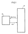
- Figure 1 shows the block diagram of a example of a device implementing the method according to the invention for the dynamic scheduling of industrial production for example.
- This device includes an OR computer coupled to a SY production system.
- This production system SY supplies to an input of the computer SY the parameters necessary for determining a scheduling: the identity ID K of each task, and the possible period T K of each task, and the definition R L of each constraint to satisfied. These parameters are provided whenever a change occurs in the nature of the tasks to be performed or in the constraints.
- the computer determines a new permutation PER, and the production system SY then performs the tasks according to this new permutation.
- the OR computer must also be programmed to transmit to each device a information telling him when he can run a spot. Programming the OR computer to put it implement the method according to the invention and for the transmission of information to each device is at the scope of the skilled person, and will not be described beyond the description of the process itself.
- the means materials for coupling an OR computer to a SY system comprising different devices capable of producing respectively different tasks is within the reach of Man art.
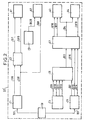
- FIGS 2 and 3 show a control system industrial requiring static scheduling. This application is considered as an example to put implementing the method according to the invention, but this is not not limited to applications where scheduling is static. The same steps make it possible to determine in real time a dynamic scheduling.
- the initialization circuit C0 is susceptible to issue information ID1 and information ID5.
- Each sensors C1 to C5 is likely to emit information.
- a C2 sensor is susceptible to issue information ID7 and information D15.
- Some sensors may receive certain information.
- sensor C2 is likely to receive ID6 information or ID8 information.
- the regulation circuits C6 and C7 are also likely to send and receive information.
- the actuators A1, A3, A4 and the display A2 are only likely to receive information.
- actuator A1 is likely to receive ID7 information and ID15 information emitted by the sensor C2.
- the same information can be received simultaneously by several elements of the system. For example, the ID8 information provided by the C1 sensor is received simultaneously by sensor C2 and by the C7 regulation.
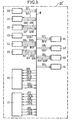
- Figure 3 shows the block diagram of this example system, to show physical connections carrying information ID1, ..., ID20. All the information is transmitted by a single medium B which is a so-called field bus passing near each equipment.
- each of the elements C0, ..., C7, A1, ..., A4 operates with a repetition period.
- these periods are respectively: 200 ms, 200 ms, 500 ms, 400 ms, 40 ms, 40 ms, 40 ms, 200 ms, 400 ms, 40 ms, 40 ms.
- the system therefore operates according to a macro-cycle having a duration equal to the least common multiple of these periods, i.e. 400 ms.
- the constraint R26: ID5 delay [0.400] requires that the transmission of information ID5, which is provided by an output of the initialization circuit C0, begins within a delay between 0 and 400 ms after a reference time absolute which is the initialization instant defined by circuit C0 and which triggers a macro-cycle.
- ID6 after ID5 [102,200] requires that the transmission of information ID6, which is supplied by the sensor C1, only starts within a delay of between 102 and 200 ms after the start of transmission of the ID5 information.
- Each constraint relates only to the start time of the transmission, which must be included in the interval indicated [t min , t max ]. Transmission can continue beyond the limit of this interval, it must only respect the fixed duration.
- the set of constraints R1, ..., R33 which relate to ID1, ..., ID20 information transmission tasks can be represented by a graph called graph of successions, in which each node represents a task and each arc connecting two nodes represents a constraint. Each arc is oriented from a node, called the predecessor, to a node corresponding to the task to which the constraint, and which must therefore be executed after the task said predecessor corresponding to the predecessor node.
- a preliminary step of the process according to the invention consists in reducing the number of permutations to be checked, by only checking the scheduling of tasks during one micro cycle which is the greatest common divisor of all task repetition periods. Indeed, if we arrive find a permutation such that if all tasks are executed during the same micro-cycle and that they satisfy all constraints, then this permutation will not cause any conflict during any of the micro-cycles constituting a macro-cycle, since the worst case is that where all the tasks fall into the same micro-cycle because of the coincidence of multiples of their periods.
- Figures 4 and 5 illustrate this preliminary step of the method according to the invention. It should be noted that in the case where one or more tasks are not considered a priori as repetitive, just assign them a value of common period chosen arbitrarily but as it facilitates the determination of a micro-cycle. So just determine the value of the greatest common divisor of repetitive task periods then choose a multiple of this value to constitute a period common to all non-repetitive tasks.
- FIGS 4 and 5 illustrate an example where schedule 6 periodic T1, ..., T6 tasks, respectively with periods equal to 10 ms, 20 ms, 30 ms, 40 ms, 50 ms, 40 ms.
- the execution time is uniform for all tasks and is equal to 1 ms.
- Figure 4 shows in gray the time intervals [t min , t max ] for each of these tasks.
- TA1 [t min , t max ] [0.4 ms] modulo 10 ms TA2 [10, 13 ms] modulo 20 ms TA3 [20, 23 ms] modulo 30 ms TA4 [30, 32 ms] modulo 40 ms TA5 [40, 41 ms] modulo 50 ms TA6 [20, 22 ms] modulo 40 ms
- tasks TA1, TA3, TA6 must be executed during the same micro-cycle [20 ms , 30 ms ] then [120 ms , 140 ms ], etc.
- the scheduling method according to the invention is then applied in this interval [0, 10 ms].
- Figure 5 shows the scheduling of tasks thus obtained, on the interval 0 to 100 ms, the interval 100 to 600 ms not being represented but having a analogous scheduling.
- Each execution interval is shown in black.
- the 20-30 ms interval in which there may be a conflict between tasks TA1, TA3, and TA6.
- TA1 task is executed during the interval 23 to 24 ms.
- TA3 task is executed during the interval 22 to 23 ms.
- TA6 task is executed during the interval 21 to 22 ms. So there is never simultaneous execution of TA1 and TA3 or TA6, whatever the considered micro-cycle, among the 60 micro-cycles constituting the macro-cycle [0, 600ms].
- this step preliminary also consists in gathering the tasks in several independent graphs, if possible, each graph gathering only tasks linked together by constraints. Scheduling multiple graphs independently is faster than scheduling a single more complex graph.
- Figure 6 shows the succession graph for the tasks performed in the system represented on the Figures 2 and 3.
- the nodes corresponding to the tasks are gathered in 6 successive layers L1 ... L6.
- the constraints R26, R12, R11, R10, R9, R1, R33 are time constraints counted from an instant of absolute reference DM which is the beginning of the micro-cycle.
- the layer L1 comprises the nodes representing the tasks of transmission of information ID5, ID12, ID11, ID10, ID9, ID1, ID20.
- the L2 layer includes the nodes corresponding to the information transmission tasks ID8, ID2, ID14, ID13.
- the L3 layer comprises the nodes corresponding to the tasks of transmission of ID6 and ID16 information.
- L4 layer includes the nodes corresponding to the transmission tasks ID15 and ID3 information.
- L5 layer contains the nodes corresponding to the transmission tasks of information ID7, ID17, ID18, ID19.
- L6 layer has only the node corresponding to the transmission task ID4 information.
- the method according to the invention determines a layer by layer scheduling, successively in order increasing rows, L1, L2, ..., L6 corresponding to successions imposed by constraints.
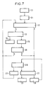
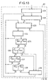
- FIG. 7 shows the flowchart of an example of the implementation process according to the invention.
- a step preliminary EO consists in determining the graph of estates arising from constraints on tasks to schedule, that is to say to gather the tasks into one number of subsets making up the layers of the graph, according to the successions imposed by the constraints. The special case where there are tasks repetitive will be explained later.
- Any task is assigned to a first layer if it is subject only to constraints of the delay type with respect to an initialization instant.
- Any task is assigned to a rank 2 layer if it is subjected to at least one type constraint after a task assigned to the rank 1 layer, and if it is not subjected to any type constraint after a task which does not has not yet been assigned to a layer, and which therefore belongs to a layer of rank greater than 1, and which can for example be the layer of rank 2.
- the layers are formed according to the rows croissants, repeating the scan of the list of constraints and eliminating from this list the constraints dealing with tasks that have been assigned to a layer.
- Any task is assigned to the layer of rank i> 1 if it is subjected to at least one type constraint after a task which has been assigned to the layer of rank i-1 and if it is not subjected to any type of constraint after a task that has not yet been assigned.
- rank i is incremented and the list of constraints is rescheduled until all the tasks have been allocated.
- a first step E1 determines the time intervals at which the execution of the tasks constituting the first layer of the graph must begin respectively.
- the limits of each of these time intervals are given directly by the values of the parameters of a constraint of the delay type. It is therefore not necessary to calculate the absolute value of the instants which limit these time intervals, for the first layer.
- a step E2 consists in scheduling all the tasks belonging to a layer, called the current layer, verifying that this scheduling is compatible with the any orders previously made for others layers. Indeed, step E2 is repeated for others layers as the first layer, as it will appear in the after. Step E2 will be described in detail below, with reference to referring to figure 13.
- step E2 determines if there is a layer after the current layer. If there is no next layer, a step E4 concludes that the scheduling of all the tasks of the graph considered is successfully completed. If there is a next layer, this one becomes the current layer and a step E5 brings together the data constituting the constraints relating to the tasks constituting this next layer.
- a step E6 calculates the limits of the time intervals [t min , t max ] where the execution of the tasks constituting the current layer must begin respectively. This calculation is described below, with reference to FIG. 4. If the calculation of a time interval for each of the tasks is a success, noted S, the method then consists in repeating step E2 to schedule the tasks belonging to the current layer. If the calculation of at least the time interval for at least one task concluded at an empty interval, step E6 is a failure, noted F. This case will be illustrated below with reference to FIG. 4. Then the method consists of an E7 test which determines whether the current layer is the first layer.
- a step E8 concludes that the scheduling has failed, because it is not possible to modify anything upstream of the first layer. If the current layer is not the first layer, then the method consists in performing a step E9 to determine a layer of rank lower than the current layer and in which the ordering will be modified to remedy the failure of the scheduling in the current layer. The layer thus determined by step E9 becomes the current layer.
- the test E7 is also carried out in the event of failure denoted F, the scheduling of the current layer by step E2. In this case, there is an incompatibility between the intervals [t min , t max ] of at least two tasks of the current layer. It is not the same type of conflict as in the case of a failure of step E6, but it too requires reordering of at least one layer of rank lower than that of the current layer.
- Step E9 determines this layer by considering what are the unfulfilled constraints. For each of these constraints, there is a predecessor task that belongs to a layer having been previously scheduled. If there is several constraints unsatisfied, step E9 determines for each layer which contains the predecessor task, then determine which of these layers has the highest rank high, to minimize the number of layers to be reordered.
- step E9 determines for the constraint dissatisfied corresponding to the layer thus determined, the direction and duration of a displacement from the start time performing this predecessor task, such as the unsatisfied constraint can be satisfied during a subsequent reordering of the current layer.
- a step E10 then consists in checking whether it is possible to obtain the time difference determined by the step E9, by modifying the permutation which has been determined previously by step E2 for this layer determined by step E9.
- step E10 concludes that it is possible to carry out this time difference, by means of a modification of the permutation which has been determined for the determined layer by step E9, then a step E11 determines a new initial permutation by making this modification.
- step E2 is repeated for reordering the current layer from this new initial permutation.
- step E10 concludes that it is not possible get this time shift by changing the permutation initial it is a failure for the layer determined by the step E9.
- the E7 test determines whether the layer which has been determined by step E9 was the first layer or not. Yes this is the first layer, step E8 concludes that the scheduling of the whole graph has failed. If this is not the first layer, step E9 is repeated for determine another layer in which the scheduling will be redetermined from an initial permutation modified.
- Step E9 searches for a layer to modify, successively considering the layers corresponding to unsatisfied constraints, according to their decreasing rank at from the current layer.
- Step E9 determines the layer on which the E2 scheduling procedure must be restarted from a new initial permutation, in taking into account the nature of the conflict which prevented the successful scheduling in the layer considered. Yes it is a conflict between a task in the current layer and a other task of the same layer, step E9 proposes to modify the permutation for the scheduling procedure of the current layer.
- a new permutation constitutes the initial permutation.
- FIG. 8 illustrates step E1 and step E6 of the scheduling method. It represents the beginning DM of the macro-cycle of a graph, such as that represented on figure 6, comprising layers n ° 1, ..., m, ..., n, p, q.
- Each of the tasks of layer n ° 1 is subjected to a single constraint which is of the delay type counted from the start DM of the macro-cycle.
- the task G must satisfy a constraint R G which imposes that the instant t G deb , where the execution of this task G begins, is included in an interval [t G min , t G max ].
- the instant t G deb can be confused with the upper limit t G max .
- a small black rectangle represents the time interval occupied by the execution of the task.
- one or more constraints of the type after may impose that the start time of execution of this task is included in a time interval determined with respect to a predecessor task.
- a task referenced K in layer n ° p Layers 1, ..., m, ..., n are assumed to have been scheduled previously. The layer n ° p is being scheduled, and the layer n ° q is not yet scheduled.
- Task K must satisfy three constraints R K1 , R K2 , R K3 , which are of the type after .
- the constraint R K1 requires that the execution of the task K begins in a time interval which is defined by two duration values which are referenced with respect to the instant t 1 where the execution of a given task of the layer no.
- the constraint R K2 requires that the execution of the task K begins in an interval defined by two duration values referenced with respect to the instant t 2 where the execution of a given task of the layer n ° m begins.
- the constraint R K3 requires that the execution of the task K begins at an instant comprised in an interval defined by two duration values referenced with respect to the instant t 3 where the execution of a given task of the layer n begins ° n.
- Constraints of type after are given with values such that the execution interval of the predecessor task cannot overlap with the execution interval of the task undergoing the considered constraint. Under these conditions, if the scheduling of a layer satisfies all the constraints relating to the tasks of this layer, it is not necessary to verify that this scheduling also satisfies other constraints relating to the layers of lower rank.
- Step E6 of the method consists in determining absolutely, by referring to the instant DM at the start of the macro-cycle, the limits of each of these three intervals. It thus determines three intervals [t K1 min , t K1 max ] [t K2 min , t K2 max ], and [t K3 min , t K3 max ]. Since task K must simultaneously satisfy the three constraints R K1 , R K2 , R K3 , the start of execution of this task K must be included in an interval [t K min , t K max ] which is the intersection of these three intervals.
- the new scheduling in layer n ° makes it possible to make the constraints R K1 , R K2 , R K3 compatible with each other, that is to say to determine a non-empty interval [t K min , t K max ], then the number of layers in which the scheduling is redetermined is limited to one.
- step E6 of the method determines a scheduling of these tasks.
- Figures 9 to 12 illustrate the basic principles of the procedure applied during step E2. This procedure order all tasks belonging to the same layer, minimizing the number of permutations to check. This procedure is successfully completed if it has determined a permutation constituting a satisfactory scheduling all the constraints relating to the tasks of this layer.
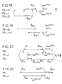
- FIG. 9 represents a timing diagram illustrating a first basic principle of the method according to the invention for scheduling tasks within the same layer.
- This first principle imposes to execute in priority the tasks for which the time interval begins the earliest, that is to say with a value t min the smallest.
- the initial permutation of the tasks that is to say the first permutation to be verified, will be constituted by a sequence referenced MIN-SUITE, in which the tasks are arranged according to the increasing order of the values of t min .
- FIG. 9 shows by rectangles IDA and IDB two time intervals allocated respectively to the execution of a task A and to the execution of a task B. Constraints impose that the task A begins to be executed at the within an interval [t A min , t A max ] or, at the limit, at time t A max . They require that task B begins to be executed within an interval [t B min , t B max ] or, at the limit, at time t B max . In this example t A min is less than t B min .
- the first basic principle consists in executing task A first, by shifting the interval during which this execution lasts, as close as possible to the lower bound t A min ; then to execute task B during an IDB interval starting as close as possible to the lower bound t B min without overlapping the IDA interval.
- FIG. 10 represents, on the same example, the consequences of a non-application of this basic principle, that is to say to execute task B before task A.
- the execution interval IDB then begins as soon as possible, that is to say at the lower limit of the interval [t B min, t B max].
- the IDA execution interval should start after the end of the IDB execution interval so as not to overlap the IDA interval, but in this example the IDB execution interval has a length such that it exceeds the instant t A max which constitutes the upper limit of the interval where it is allowed to start the execution of task A.
- the overlap area is hatched in Figure 6.
- FIG. 11 represents a timing diagram illustrating a second basic principle of the method according to the invention, for scheduling tasks within the same layer.
- This basic principle makes it possible to choose which task is to be executed in priority among several tasks for which the lower bound t min has the same value.
- This second principle requires, in this case, to execute in priority the task for which the upper limit t max is the smallest.
- the upper bound t B max is greater than the upper bound t A max corresponding to task A.
- Figure 12 illustrates on the same example, a conflict which is more likely to occur if the second principle is not respected.
- Task B is executed first, from time t B deb which coincides with the end t 0 of the forbidden interval represented by hatching.
- Step E2 firstly consists of a step E21 consisting in determine the MIN-SUITE sequence made up of all the tasks of the current layer, ordered according to the values increasing from the lower bound tmin. This sequel will used to apply the first principle stated previously.
- the initial permutation is constituted by MIN-SUITE; and the permutations which will be checked next, by in case of failure, will be deducted from MIN-SUITE, by successive modifications.
- step E21 consists in determining the MAX-SUITE sequence, consisting of all the tasks of the current layer, ordered according to the increasing values of the upper bound t max . This sequence will be used to apply the second principle stated above, when it will be necessary to modify the initial permutation.
- a step E22 consists in checking the permutation current, i.e. check if it satisfies all constraints on the tasks of the current layer.
- the current permutation is constituted by the initial permutation determined by step E21.
- This verification consists in successively taking each task in the order of the current permutation and in verifying that the execution interval [t deb , t end ] imposed by the position occupied by this task in the current permutation is compatible with the time interval [t min , t max ] imposed by the constraints relating to this task.
- the task for which this check is in progress is called the current task. If this verification is positive for each of the tasks of the current permutation, this means that the current permutation is a success, denoted S, and the scheduling can continue by step E3 of the flow chart represented in FIG. 7.
- step E22 finds a task, noted X, which is the first misplaced in the current permutation, it draws the conclusion, noted R, that it is necessary to seek a candidate candidate for a displacement to constitute a new permutation.
- the method then consists in executing a step E23 which searches for the task immediately preceding the current task X in the MAX-SUITE sequence. If there is no such task, step E23 ends in failure, denoted F, and the method then consists in performing step E7 of the flowchart shown in FIG. 7.
- step E23 finds a candidate task Q preceding immediately the current task X in the MAX-SUITE suite, the process then consists of a step E24 verifying that this task Q has already been considered well placed, during from a previous step E21. All the tasks that are considered to be well placed are those that have a rank lower than that of the current task X, since the verification of step E22 is done according to the ranks increasing in the current permutation. Therefore, step E24 simply consists in verifying that the task candidate Q precedes current task X in permutation current. If step E24 determines that task Q has not been considered to be well placed, step E23 is repeated for search for another candidate task, immediately preceding the Q task in MAX-SUITE.
- the method consists in executing a step E25 which consists in comparing the instant t Q deb of the start of execution of the task Q with the instant t X max which is the upper bound of the time interval corresponding to the current task X.
- step E29 consisting in moving the task Q in the current permutation, to insert it between the current task X and the task following the task X in the current permutation.
- the tasks which were placed between Q and X, and the task X itself, are shifted by one row, towards the lower rows, to fill the space left free by Q. Consequently, task Q now occupies the position which was that of X.
- the method then consists in repeating step E22 to verify whether the new current permutation thus obtained satisfies all the constraints of the layer considered. It should be noted that task Q and all the other tasks that followed it have been moved.
- FIG. 14 illustrates by an example the case ⁇ .
- the execution intervals are shown in dotted lines when a conflict prevents execution, and in features continuous otherwise.
- Figure 15 shows that by moving the tasks Q and X respectively in the positions PS i-1 and PSj, the probability that the instant t deb (PS i-1 ) falls in the interval [t X min , t X max ] is greater than the probability that the instant t deb (P si ) had to fall in this same interval, because t deb systematically believes with the rank of the position PS.
- the figure shows that the end t X max of the segment corresponding to task X has approached an execution interval, the one that begins at time t deb (PSi-1), and therefore has more chances to have an intersection with such an interval.
- the end t Q max of the segment corresponding to task Q has non-zero chances of having an intersection with the rectangle representing the execution interval starting at time t deb (PSi). Therefore, the new permutation is more likely than the old one to satisfy all the constraints and it is therefore useful to try this new permutation.
- t deb (PS i-1 ) falls beyond t max , so there is still a conflict for task X. It is therefore necessary to make one or more other modifications to the current permutation .
- step E26 This consists in comparing the instant t Q end of the end of execution of the task Q, with the instant t X max which is the upper limit of the interval where the execution of the task X must begin. If t Q end ⁇ t X max, this case is noted ⁇ , and the method then consists in carrying out step E30 which moves the task Q and inserts it after the task X. The opposite case is noted ⁇ .
- Other checks are necessary before being able to conclude that task Q is an interesting candidate task.
- FIG. 16 represents a task X in the position PS i and a task Q in the position PSj, such as the case ⁇ and the case ⁇ are realized: the instant t Q end of the end of execution of the task Q, that is to say the instant t end (PSj) imposed by the position PSj of Q in the current permutation , is located beyond the instant t X max .
- step E27 consists in comparing the instant t Q max which is the upper bound of the time interval at which the execution of the task Q must begin, at the instant t X max which is the upper bound of l time interval at which the execution of task X must begin. If t Q max > t X max , this case is noted ⁇ , and the method then consists in then performing a step E28. Otherwise noted ⁇ , and the method then consists in repeating step E23 because the candidate task Q has no chance of being interesting.
- Figures 18 and 19 illustrate by example the case ⁇ .
- the limit t Q max is strictly less than the instant t X max .
- FIG. 18 represents the tasks X and Q displaced respectively in the positions PS i-1 and P si .
- This figure 18 shows that the instant t Q max becomes closer to the instant t (PSi) deb than it was to the instant t (PSj) deb but the task Q has no chance of being able to be executed because t Q max is even further from t (PSi) deb than t Q max was . Since task Q is 100% likely to be misplaced, it is useless to try such a modification of the current permutation, this is why the next step is a step E23 of searching for another candidate task for a relocation.
- step E28 consists in comparing the instant t Q min which is the lower bound of the interval in which the execution of the task Q must begin, with the instant t X min which is the bound lower the time interval in which the execution of task X should begin.
- step E28 The purpose of this step E28 is to verify that the task Q is placed before the current task X in the MIN-SUITE suite, in order to be able to move the task Q after the task X. Otherwise, noted ⁇ , the next step is a step E23 of searching for another candidate task for a displacement.
- next step is a step E29 moving task Q after task X; then a step E22 is reiterated to check whether all the constraints relating to the tasks of the current layer are satisfied.
- Fig 20 illustrates an example where the cases ⁇ , ⁇ , ⁇ , ⁇ , are performed simultaneously.
- FIG. 21 represents the tasks X and Q displaced respectively in the positions PSi-1 and PSi, in an example where the constraints are such that they are effectively satisfied after this displacement: t deb (PSi) falls in the interval [t Q min , t Q max ] and t deb (PSi-1) fall in the interval [t X min , t X max ].
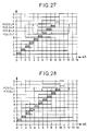
- Figures 22 to 31 illustrate the realization of step E2 to schedule an example of a layer comprising 13 tasks: A, B, C, D, E, G, J, K, L, N, P, S, T.
- Figure 22 shows on a time scale from O to 14 ms, the position of the corresponding execution intervals respectively at 13 positions PS1, ..., PS13.
- the tasks are executed in the order of positions PS1, ..., PS13, and each execution interval has a duration equal to 1 ms.
- Each task must satisfy one or more constraints that result in a single constraint: the beginning the execution interval (black rectangle in figure 22) must be located in a given time interval (segments black in Figure 23). In a borderline case it can start to the upper bound.
- Step E21 consists in determining the MIN-SUITE sequence consisting of all the tasks of the current layer, ordered according to the increasing values of the lower bound t min .
- MIN-SUITE N, J, S, D, E, B, T, A, K, P, L, C, G.
- the 13 tasks are represented in the order of MIN-SUITE, according to the direction of orientation of the axis ordinates.
- the so-called initial permutation which will be checked in first will be that constituted by MIN-SUITE; and those who will be checked next, in case of failure, will be deducted from MIN-SUITE by successive modifications.
- step E21 consists in determining the MAX-SUITE sequence, consisting of all the tasks of the current layer, ordered according to the increasing values of t max .
- This sequence will be used to apply the second principle stated above, when it will be necessary to modify the initial permutation.
- MAX-SUITE N, S, J, T, G, C, L, B, P, K, A, D, E.
- a step E22 consists in checking the permutation current, i.e. check if it satisfies all constraints on the tasks of the layer considered.
- the current permutation is constituted by the initial permutation determined by the step E21.
- the verification is done successively for each task, in the order of the current permutation: N, J, S, D, E, ..., G. If the verification is positive for a task this is considered to be well placed in the permutation, but its placement can be called into question later if necessary to satisfy other constraints.
- FIGS. 22 and 23 make it possible to conclude that there is no problem in executing tasks N, J, S, and D, respectively during the execution intervals represented in FIG. 22. They are therefore considered as well placed.
- the current permutation is: N J S D EBTAKPLCG where tasks considered to be well placed are underlined.
- Figure 24 illustrates the first conflict encountered during the verification of the initial permutation.
- black rectangles represent execution intervals for which there is no conflict between the constraints, and a dotted white rectangle represents the execution interval which is the cause of a conflict. It corresponds to position PS5, currently occupied by task E. This execution interval has nothing in common with the interval in which the execution of task E must begin.
- Step E23 then consists in searching in the MAX-SUITE sequence a task preceding task E, that is to say such that the limit t max has a higher value.
- MAX-SUITE N, S, J, T, G, C, L, B, P, K, A, D, E.
- Step E23 finds task D.
- Step E24 verifies that it is considered to be well placed, by verifying that it has a rank lower than the rank of the current task E, in the current permutation.
- step E25 draws a conclusion ⁇ .
- step E26 draws a conclusion ⁇ .
- Step E29 then moves D to the POS5 position and E moves back to the POS4 position.
- Step E22 verifies that the constraints relating to E and the following tasks are satisfied but notes that the constraints relating to D are no longer satisfied. The permutation tried is not suitable. It is not retained as a new current permutation.
- Step E23 would then find as a candidate task successively: A, K, P, B, L, C, G, T, J; and step E24 would retain task J.
- MAX-SUITE N, S, J, T, G, C, L, B, P, K, A, P.
- step E23 finds as candidate task successively A, K, P, B, L, C, G, T, which are rejected by step E24. Then step E23 finds task J.
- Step E24 verifies that the task J is considered to be well placed.
- Step E25 comes to the conclusion ⁇ .
- Step E26 comes to the conclusion ⁇ .
- Steps E27 and E28 arrive at the conclusion ⁇ and ⁇ . Consequently step E29 places task J in position PS5, in place of E.
- Tasks E, D and S move back one place, S being in position PS2, D in position PS3, and E in the PS4 position. The other tasks do not change places.
- Step E22 then consists in verifying that the tasks who have been moved check all constraints dealing with them, starting with the highest ranking task low among those displaced: S, then E, then D, then J. Elle then check that there is no conflict between constraints successively for tasks B, T, A, K.
- Figure 26 illustrates the new current permutation. It should be noted that for task K the execution interval begins at the exact moment when the interval in which the execution of task K must begin begins. There is no conflict, but the constraints are narrowly met.
- the state of the current permutation is: N , S , E , D , J , B , T , A , K , P, L, C, G.
- Step E23 then successively finds the tasks L, C, G but step E24 rejects them because they are not considered to be well placed in the permutation. Finally steps E23 and E24 find task T. Steps E25 to E28 successively draw conclusions ⁇ , ⁇ , ⁇ , ⁇ . Step E29 moves T to position POS10. Tasks P, K, A move back respectively to positions POS9, POS8, POS7.
- Step E22 then verifies that the constraints relating to the displaced tasks A, K, P, T, and the following ones, are satisfied.
- the new current permutation is: N , S , E , D , J , B , A , K , P , T , L, C, G
- step E22 notes then that the constraints relating to the task L are not not satisfied.
- Step E23 finds task T and step E24 verifies that it is considered to be well placed. Step E25 and the following ones can therefore be executed. They draw conclusions ⁇ , then ⁇ , then ⁇ and ⁇ . Step E29 can then be executed. It places task T in position PS 11 which was occupied by task L. Task L moves back one place. Step E22 verifies that the constraints relating to the displaced tasks L and T are satisfied. Therefore the current permutation becomes: N , S , E , D , J , V , A , K , P , L , T , C, G
- the new current permutation is: N , S , E , D , J , B , A , K , P , L , C , T , G
- step E22 finds that there is a conflict between the constraints relating to task G.
- Step E23 determines a task, T, which precedes task G immediately in the MAX-SUITE sequence .
- Step E24 verifies that the task T is considered to be well placed in the permutation.
- Step E29 moves T after G in the permutation, which amounts to permuting T and G.
- step E22 verifies that all the constraints relating to the displaced tasks G and T are satisfied.
- the new current permutation is: N , S , E , D , J , B , A , K , P , L , C , G , T.
- step E2 is ends with a success S. If there are other layers of rank higher, their scheduling continues with step E3 of the flowchart shown in Figure 7.
Landscapes
- Engineering & Computer Science (AREA)
- Software Systems (AREA)
- Theoretical Computer Science (AREA)
- Physics & Mathematics (AREA)
- General Engineering & Computer Science (AREA)
- General Physics & Mathematics (AREA)
- Management, Administration, Business Operations System, And Electronic Commerce (AREA)
- Vehicle Body Suspensions (AREA)
- Two-Way Televisions, Distribution Of Moving Picture Or The Like (AREA)
- Control Of Steam Boilers And Waste-Gas Boilers (AREA)
- Control By Computers (AREA)
- Mobile Radio Communication Systems (AREA)
- Paper (AREA)
- Data Exchanges In Wide-Area Networks (AREA)
- Feedback Control In General (AREA)
- Position Fixing By Use Of Radio Waves (AREA)
- Time-Division Multiplex Systems (AREA)
- General Factory Administration (AREA)
Abstract
Description
L'invention concerne un procédé pour ordonnancer des tâches successives, au moyen d'un ordinateur, en déterminant un ordre d'exécution de ces tâches et un instant de début d'exécution pour chaque tâche, deux tâches ne devant jamais être exécutées simultanément. Cet ordonnancement est réalisé en fonction d'une pluralité de contraintes que doivent satisfaire les tâches. Ce procédé concerne plus particulièrement les applications où il y a deux types de contrainte :
- Des contraintes de succession : une tâche doit être exécutée après une ou plusieurs autres tâches prédéterminées.
- Des contraintes de délais : l'exécution d'une tâche doit commencer à un instant compris dans au moins un intervalle de temps prédéterminé. Cet intervalle est généralement déterminé par rapport à l'instant de début d'exécution d'une tâche qui doit précéder immédiatement la tâche considérée, ou par rapport à un instant de référence absolue. Une tâche qui précède immédiatement la tâche considérée est appelée tâche prédécesseur. Le nombre de tâches prédécesseurs n'est pas limité.
- Succession constraints: a task must be executed after one or more other predetermined tasks.
- Time constraints: the execution of a task must start at a time included in at least a predetermined time interval. This interval is generally determined in relation to the start time of execution of a task which must immediately precede the task considered, or in relation to an absolute reference time. A task that immediately precedes the task in question is called the predecessor task. There is no limit to the number of predecessor tasks.
Le procédé selon l'invention est applicable notamment à des tâches qui doivent être exécutées successivement parce qu'elles sont exécutées par un moyen unique capable de n'exécuter qu'une seule tâche à la fois, par exemple : une machine outil, un bus informatique, ou une équipe de travailleurs. Dans le domaine de l'informatique, il peut être appliqué à la gestion d'une pluralité de tâches prédéterminées à exécuter successivement dans un même processeur ou sur un même bus. Dans le domaine du contrôle-commande industriel, il peut être appliqué notamment à la gestion d'un bus dit de terrain, utilisé pour transmettre des informations successivement selon un ordonnancement prédéterminé.The method according to the invention is applicable in particular to tasks that must be performed successively because that they are executed by a unique means capable of perform only one task at a time, for example: a machine tool, a computer bus, or a team of workers. In the IT field, it can be applied to the management of a plurality of tasks predetermined to execute successively in the same processor or on the same bus. In the field of control-command industrial, it can be applied in particular to the management of a so-called field bus, used to transmit information successively according to a schedule predetermined.
De nombreux procédés d'ordonnancement sont déjà connus :
- les méthodes dites pôlynomiales ou de circuits critiques;
- les méthodes de programmation linéaire, notamment la méthode du simplex, sur laquelle est fondée le langage PROLOG III;
- les méthodes de programmation dynamique, qui ne peuvent être appliquées qu'à des problèmes de taille assez faible;
- et les méthodes heuristiques, qui utilisent certains algorithmes des méthodes citées ci-dessus, mais qui consistent en outre à réduire le nombre de cas à vérifier, en simplifiant certaines contraintes; la solution obtenue étant alors non optimale.
- the so-called polynomial or critical circuit methods;
- linear programming methods, in particular the simplex method, on which the PROLOG III language is based;
- dynamic programming methods, which can only be applied to fairly small problems;
- and heuristic methods, which use certain algorithms of the methods mentioned above, but which also consist in reducing the number of cases to be verified, by simplifying certain constraints; the solution obtained then being non-optimal.
Les procédés connus ont deux inconvénients : ils nécessitent une durée de calcul importante parce qu'ils vérifient systématiquement un très grand nombre de permutations avant de fournir une solution. La durée de calcul est généralement proportionnelle à la fonction factorielle du nombre de tâches à ordonnancer.The known methods have two drawbacks: they require a significant calculation time because they systematically check a very large number of permutations before providing a solution. The duration of calculation is generally proportional to the function factorial of the number of tasks to schedule.
Pour ordonnancer des tâches répétitives, les procédés connus déterminent la durée d'un macro-cycle égal au plus petit commun multiple de toutes les périodes des tâches, et déterminent la durée d'un micro-cycle égal au plus grand commun diviseur de toutes les périodes des tâches, puis ils cherchent une permutation des tâches telle que toutes les contraintes soient satisfaites simultanément, en essayant toutes les permutations possibles jusqu'à en trouver une vérifiant cette condition, en faisant les vérifications micro-cycle par micro-cycle. Lorsqu'un conflit apparaít dans un micro-cycle la permutation en cours de vérification est abandonnée, et une autre est essayée. Le travail effectué pour la vérification de cette permutation pendant les micro-cycles précédents devient inutile parce que toutes les contraintes satisfaites précédemment sont remises en cause.To schedule repetitive tasks, the procedures known determine the duration of a macro-cycle equal to at most common multiple of all task periods, and determine the duration of a micro-cycle equal to the largest common divisor of all task periods and then they seek a permutation of tasks such that all constraints be satisfied simultaneously, trying all possible permutations until you find one checking this condition, doing the checks micro-cycle by micro-cycle. When a conflict arises in a micro-cycle the permutation being checked is abandoned, and another is tried. The work done for the verification of this permutation during the micro-cycles precedents become useless because all constraints previously satisfied are called into question.
Les procédés connus sont donc peu pratiques à mettre en oeuvre dans des applications industrielles. The known methods are therefore impractical to implement works in industrial applications.
Le but de l'invention est de proposer un procédé d'ordonnancement qui n'ait pas ces inconvénients, afin d'obtenir plus rapidement une solution à un problème d'ordonnancement statique, mais aussi pour permettre de traiter des problèmes d'ordonnancement dynamique, c'est-à-dire redéterminer un ordonnancement au fur et à mesure de l'évolution du nombre de tâches à ordonnancer et de l'évolution des contraintes portant sur ces tâches. Un tel ordonnancement dynamique peut être utile par exemple pour ordonnancer des tâches d'usinage sur une machine outil, lorsque les produits à fabriquer sont très diversifiés; pour ordonnancer les décollages ou les atterrissages d'avions sur une piste d'aéroport; pour ordonnancer des tâches sur un bus ou un processeur informatique; etc.The object of the invention is to propose a method scheduling that doesn't have these drawbacks, so get a solution to a problem faster static scheduling, but also to allow deal with dynamic scheduling problems, i.e. redetermine a scheduling as and when the evolution of the number of tasks to be scheduled and the evolution of the constraints relating to these tasks. Such dynamic scheduling can be useful for example for schedule machining tasks on a machine tool, when the products to be manufactured are very diverse; for schedule aircraft takeoffs or landings on an airport runway; to schedule tasks on a bus or a computer processor; etc.
L'objet de l'invention est un procédé pour ordonnancer
des tâches successives au moyen d'un ordinateur, certaines
tâches devant satisfaire des contraintes; les contraintes,
pour une tâche, consistant en ce que l'instant t K deb de début
d'exécution doit être compris dans au moins un
intervalle de temps [tkmin, tkmax] prédéterminé par rapport
à l'instant de début d'exécution d'une autre tâche, appellée
prédécesseur, dont l'exécution précède celle de la tâche
considéré; ou bien prédéterminé par rapport à un instant de
référence absolue;
caractérisé en ce qu'il consiste à :
- considérer que toutes les tâches sont répétitives, et à réduire l'intervalle de temps sur lequel l'ordonnancement est à déterminer, en réduisant cet intervalle à un micro-cycle dont la durée est égale au plus grand commun diviseur de toutes les périodes de répétition des tâches; et en recherchant un ordonnancement tel que si toutes les tâches sont exécutées au cours d'un même micro-cycle elles satisfassent toutes les contraintes;
- rassembler les tâches à exécuter, dans des couches en fonction des successions imposées par les contraintes;
- ordonnancer les tâches couche par couche, dans l'ordre des couches de rangs croissants, jusqu'à la dernière couche si c'est possible; et conclure alors que l'ordonnancement obtenu est bon;
- refaire l'ordonnancement d'une couche qui est la couche de rang le plus élevé parmi les couches contenant respectivement les tâches prédécesseurs correspondant aux contraintes non satisfaites, en dicalant l'instant d'exécution de la tâche prédécesseur contenue dans cette couche avec un sens et une durée tels que la contrainte insatisfaite pourra être satisfaite lors d'un réordonnancement ultérieur de la couche courante;
- puis à faire, ou éventuellement refaire, l'ordonnancement de toutes les autres couches ayant un rang supérieur à celui de la couche de la tâche prédécesseur, jusqu'à la dernière couche, si c'est possible, et à conclure alors que l'ordonnancement obtenu est bon.
characterized in that it consists of:
- consider that all the tasks are repetitive, and to reduce the time interval over which the scheduling is to be determined, by reducing this interval to a micro-cycle whose duration is equal to the greatest common divisor of all the repetition periods stain; and by looking for a scheduling such that if all the tasks are executed during the same micro-cycle they satisfy all the constraints;
- gather the tasks to be executed, in layers according to the successions imposed by the constraints;
- order the tasks layer by layer, in order of the layers of increasing rows, until the last layer if possible; and then conclude that the scheduling obtained is good;
- redo the scheduling of a layer which is the layer of the highest rank among the layers respectively containing the predecessor tasks corresponding to the constraints not satisfied, by dicalizing the instant of execution of the predecessor task contained in this layer with a meaning and a duration such that the unsatisfied constraint can be satisfied during a subsequent reordering of the current layer;
- then to make, or possibly redo, the ordering of all the other layers having a rank higher than that of the layer of the predecessor task, up to the last layer, if possible, and to conclude then that the scheduling obtained is good.
Le procédé ainsi caractérisé présente l'avantage d'être
plus rapide que les procédés connus parce :
Ces deux caractéristiques réduisent considérablement le temps de calcul, par rapport aux procédés connus qui explorent systématiquement toutes les possibilités d'ordonnancement, en remettant en cause toutes les contraintes ayant été satisfaites précédemment, lorsqu'une permutation ne satisfait pas une contrainte.These two characteristics considerably reduce the calculation time, compared to known methods which systematically explore all possibilities scheduling, by calling into question all the constraints having been satisfied previously, when a permutation does not satisfy a constraint.
Enfin, ce procédé est applicable à l'ordonnancement d'un système dans lequel plusieurs tâches peuvent être effectivement réalisées en parallèle, en décomposant ce système en plusieurs sous-systèmes parallèles dans lesquels les tâches doivent toutes être exécutées successivement; et en appliquant le procédé selon l'invention pour chacun des sous-systèmes ainsi déterminés.Finally, this process is applicable to scheduling of a system in which multiple tasks can be actually performed in parallel, by breaking down this system into several parallel subsystems in which the tasks must all be carried out successively; and by applying the method according to the invention for each of the subsystems so determined.
L'étape consistant à ordonnancer les tâches couche par couche peut être réalisée en mettant en oeuvre un procédé connu tel que l'algorithme du simplex, mais un mode de mise en oeuvre préférentiel, pour ordonnancer chaque couche, consiste à :
- calculer, pour chaque tâche de la couche courante, les bornes tmin et tmax de l'intervalle où doit commencer l'exécution de cette tâche;
- constituer une première suite dans laquelle toutes les tâches de la couche courante sont ordonnées selon les valeurs de tmin croissantes ;
- constituer une seconde suite dans laquelle toutes les tâches de la couche courante sont ordonnées selon les valeurs de tmax croissantes;
- constituer une permutation dite initiale, en ordonnançant les tâches de la couche courante dans l'ordre de la première suite;
- vérifier si la permutation initiale satisfait toutes les contraintes portant sur les tâches de la couche courante;
- conclure que l'ordonnancement de la couche courante est un succès si toutes les contraintes sont satisfaites;
- sinon, déterminer dans la permutation initiale la première tâche, dite mal placée, pour laquelle une contrainte n'est pas satisfaite;
- déterminer dans la seconde suite une tâche dite candidate qui précède immédiatement la tâche mal placée, dans cette seconde suite et qui précède aussi la tâche mal placée, dans la permutation courante;
- vérifier que, si la tâche candidate est déplacée dans
la permutation courante pour être placée immédiatement après
la tâche mal placée, toutes les contraintes portant sur les
tâches ainsi déplacées sont alors satisfaites; et
- si au moins une contrainte n'est pas satisfaite, conclure que la tâche candidate ne convient pas, puis déterminer dans la seconde suite une autre tâche candidate et réitérer la vérification précédente; et si, ce n'est pas possible, conclure que l'ordonnancement de la couche courante a échoué;
- si toutes les contraintes sont satisfaites, conclure que l'ordonnancement de la couche courante est un succès.
- calculate, for each task of the current layer, the limits t min and t max of the interval at which the execution of this task must begin;
- constitute a first sequence in which all the tasks of the current layer are ordered according to the increasing values of t min ;
- constitute a second sequence in which all the tasks of the current layer are ordered according to the increasing values of t max ;
- constitute a so-called initial permutation, by scheduling the tasks of the current layer in the order of the first sequence;
- check if the initial permutation satisfies all the constraints relating to the tasks of the current layer;
- conclude that the scheduling of the current layer is successful if all the constraints are satisfied;
- otherwise, determine in the initial permutation the first task, said to be misplaced, for which a constraint is not satisfied;
- determining in the second sequence a so-called candidate task which immediately precedes the misplaced task, in this second sequence and which also precedes the misplaced task, in the current permutation;
- check that, if the candidate task is moved in the current permutation to be placed immediately after the misplaced task, all the constraints relating to the tasks thus displaced are then satisfied; and
- if at least one constraint is not satisfied, conclude that the candidate task is not suitable, then determine in the second sequence another candidate task and repeat the previous verification; and if this is not possible, conclude that the scheduling of the current layer has failed;
- if all the constraints are satisfied, conclude that the scheduling of the current layer is a success.
Le procédé ainsi caractérisé présente l'avantage d'être particulièrement rapide parce qu'en cas d'échec pour l'ordonnancement d'une tâche de cette couche, il consiste à déplacer, à l'intérieur de cette couche, une ou plusieurs tâches précédant la tâche où l'ordonnancement est en échec, sans remettre en cause systématiquement toutes les contraintes déjà satisfaites dans cette couche, et donc sans remettre en cause l'intégralité du travail effectué précédemment dans cette couche. Cette caractéristique réduit considérablement le temps de calcul par rapport à tout procédé qui consisterait à explorer systématiquement toutes les possibilités d'ordonnancement dans cette couche.The process thus characterized has the advantage of being particularly fast because in case of failure for the scheduling of a task of this layer, it consists of move, inside this layer, one or more tasks preceding the task where the scheduling has failed, without systematically questioning all constraints already satisfied in this layer, and therefore without question all of the work done previously in this layer. This feature reduces considerably the computation time compared to everything process which would consist of systematically exploring all the scheduling possibilities in this layer.
Le procédé selon l'invention sera mieux compris et d'autres caractéristiques apparaítront à l'aide de la description ci-dessous d'un exemple de mise en oeuvre, et des figures l'accompagnant :
- la figure 1 représente le schéma synoptique d'un système dans lequel le procédé selon l'invention est mis en oeuvre pour déterminer dynamiquement un ordonnancement;
- la figure 2 représente le schéma fonctionnel d'un exemple de système de contrôle-commande industriel nécessitant un ordonnancement statique;
- la figure 3 représente le schéma synoptique de ce système de contrôle-commande industriel, comportant un bus de terrain sur lequel des informations sont transmises de manière successive, selon un ordonnancement déterminé en appliquant le procédé selon l'invention;
- les figures 4
et 5 illustrent une étape du procédé selon l'invention, pour prendre en compte le caractère périodique de certaines tâches; - la figure 6 représente un graphe dit de successions,
qui a été déterminé pour l'exemple de système représenté sur
les figures 2
et 3; - la figure 7 représente l'organigramme des étapes d'un exemple de mise en oeuvre du procédé selon l'invention;
- la figure 8 illustre une première étape de l'organigramme représenté sur la figure 7;
- les figures 9 à 12 illustrent les principes de base de l'ordonnancement des tâches à l'intérieur d'une couche du graphe de successions, selon l'invention;
- la figure 13 représente l'organigramme plus détaillé d'une étape E2 de l'organigramme représenté sur la figure 7, réalisant l'ordonnancement des tâches à l'intérieur d'une couche du graphe de successions;
- les figures 14 à 21 représentent des chronogrammes illustrant la mise en oeuvre de l'organigramme représenté sur la figure 11;
- les figures 22 à 31 illustrent la mise en oeuvre de l'organigramme représenté sur la figure 13 pour ordonnancer un exemple de couche.
- FIG. 1 represents the block diagram of a system in which the method according to the invention is implemented for dynamically determining a scheduling;
- FIG. 2 represents the functional diagram of an example of an industrial control-command system requiring static scheduling;
- FIG. 3 represents the block diagram of this industrial control-command system, comprising a field bus on which information is successively transmitted, according to a scheduling determined by applying the method according to the invention;
- Figures 4 and 5 illustrate a step in the method according to the invention, to take into account the periodic nature of certain tasks;
- FIG. 6 represents a so-called succession graph, which has been determined for the example of system represented in FIGS. 2 and 3;
- FIG. 7 represents the flow diagram of the steps of an example of implementation of the method according to the invention;
- Figure 8 illustrates a first step in the flowchart shown in Figure 7;
- Figures 9 to 12 illustrate the basic principles of the scheduling of tasks within a layer of the succession graph, according to the invention;
- FIG. 13 represents the more detailed flowchart of a step E2 of the flowchart shown in FIG. 7, performing the scheduling of the tasks within a layer of the succession graph;
- Figures 14 to 21 show timing diagrams illustrating the implementation of the flowchart shown in Figure 11;
- Figures 22 to 31 illustrate the implementation of the flowchart shown in Figure 13 to schedule an example layer.
Le procédé selon l'invention peut être mis en oeuvre aussi bien pour déterminer un ordonnancement statique, que pour déterminer un ordonnancement dynamique. Mais la réduction de la durée de calcul qu'il procure est particulièrement avantageuse pour déterminer un ordonnancement dynamique, puisqu'elle permet de prendre en compte en temps réel des changements de contraintes ou de tâche.The method according to the invention can be implemented as well to determine a static scheduling, as to determine dynamic scheduling. But the reduction in the computing time it provides is particularly advantageous for determining a dynamic scheduling, since it allows taking into account in real time of changes in constraints or task.
La figure 1 représente le schéma synoptique d'un exemple de dispositif mettant en oeuvre le procédé selon l'invention pour l'ordonnancement dynamique de tâches de production industrielle par exemple.Figure 1 shows the block diagram of a example of a device implementing the method according to the invention for the dynamic scheduling of industrial production for example.
Ce dispositif comporte un ordinateur OR couplé à un système de production SY. Ce système de production SY fournit à une entrée de l'ordinateur SY les paramètres nécessaires pour déterminer un ordonnancement : l'identité IDK de chaque tâche, et la période éventuelle TK de chaque tâche, et la définition RL de chaque contrainte à satisfaire. Ces paramètres sont fournis chaque fois qu'un changement intervient dans la nature des tâches à exécuter ou dans les contraintes.This device includes an OR computer coupled to a SY production system. This production system SY supplies to an input of the computer SY the parameters necessary for determining a scheduling: the identity ID K of each task, and the possible period T K of each task, and the definition R L of each constraint to satisfied. These parameters are provided whenever a change occurs in the nature of the tasks to be performed or in the constraints.
L'ordinateur détermine alors une nouvelle permutation PER, et le système de production SY exécute ensuite les tâches conformément à cette nouvelle permutation.The computer then determines a new permutation PER, and the production system SY then performs the tasks according to this new permutation.
Les tâches sont généralement exécutées par différents dispositifs que comporte le système SY. L'ordinateur OR doit être programmé aussi pour transmettre à chaque dispositif une information lui indiquant les instants où il peut exécuter une tâche. La programmation de l'ordinateur OR pour le mettre en oeuvre le procédé selon l'invention et pour la transmission à chaque dispositif d'une information est à la portée de l'Homme de l'Art, et ne sera pas décrite au-delà de la description du procédé lui-même. De même, les moyens matériels pour coupler un ordinateur OR à un système SY comportant différents dispositifs aptes à réaliser respectivement différentes tâches, est à la portée de l'Homme de l'Art.Tasks are usually performed by different SY system features. The OR computer must also be programmed to transmit to each device a information telling him when he can run a spot. Programming the OR computer to put it implement the method according to the invention and for the transmission of information to each device is at the scope of the skilled person, and will not be described beyond the description of the process itself. Likewise, the means materials for coupling an OR computer to a SY system comprising different devices capable of producing respectively different tasks, is within the reach of Man art.
Les figures 2 et 3 représentent un système de contrôle-commande industriel nécessitant un ordonnancement statique. Cette application est considérée à titre d'exemle pour mettre en oeuvre le procédé selon l'invention, mais celui-ci n'est pas limité aux applications où l'ordonnancement est statique. Les mêmes étapes permettent de déterminer en temps réel un ordonnancement dynamique.Figures 2 and 3 show a control system industrial requiring static scheduling. This application is considered as an example to put implementing the method according to the invention, but this is not not limited to applications where scheduling is static. The same steps make it possible to determine in real time a dynamic scheduling.
La figure 2 représente le schéma fonctionnel d'un système de contrôle-commande industriel SY'. Chaque tâche consiste à transmettre une information entre un émetteur et un récepteur, alors que le médium utilisable ne peut porter qu'une seule informatin à la fois. Ce système SY' comporte :
- un circuit d'initialisation C0;
- des capteurs C1, ..., C5;
- des circuits de régulation C6 et C7;
- des actionneurs A1, A3, A4;
- un afficheur A2.
- an initialization circuit C0;
- sensors C1, ..., C5;
- regulation circuits C6 and C7;
- actuators A1, A3, A4;
- an A2 display.
Les échanges d'information sont représentés par des flèches. Le circuit d'initialisation C0 est susceptible d'émettre une information ID1 et une information ID5. Chacun des capteurs C1 à C5 est susceptible d'émettre des informations. Par exemple un capteur C2 est susceptible d'émettre une information ID7 et une information D15. Certains capteurs sont susceptibles de recevoir certaines informations. Par exemple, le capteur C2 est susceptible de recevoir l'information ID6 ou l'information ID8.Information exchanges are represented by arrows. The initialization circuit C0 is susceptible to issue information ID1 and information ID5. Each sensors C1 to C5 is likely to emit information. For example a C2 sensor is susceptible to issue information ID7 and information D15. Some sensors may receive certain information. For example, sensor C2 is likely to receive ID6 information or ID8 information.
Les circuits de régulation C6 et C7 sont eux aussi susceptibles d'émettre et de recevoir des informations. Dans cet exemple, les actionneurs A1, A3, A4 et l'afficheur A2, sont seulement susceptibles de recevoir des informations. Par exemple, l'actionneur A1 est susceptible de recevoir l'information ID7 et l'information ID15 émises par le capteur C2. Par ailleurs, une même information peut être reçue simultanément par plusieurs éléments du système. Par exemple, l'information ID8 fournie par le capteur C1 est reçue simultanément par le capteur C2 et par le circuit de régulation C7.The regulation circuits C6 and C7 are also likely to send and receive information. In this example, the actuators A1, A3, A4 and the display A2, are only likely to receive information. Through example, actuator A1 is likely to receive ID7 information and ID15 information emitted by the sensor C2. In addition, the same information can be received simultaneously by several elements of the system. For example, the ID8 information provided by the C1 sensor is received simultaneously by sensor C2 and by the C7 regulation.
La figure 3 représente le schéma synoptique de cet exemple de système, pour montrer les liaisons physiques transportant les informations ID1, ..., ID20. Toutes les informations sont transmises par un support unique B qui est un bus dit de terrain passant à proximité de chaque équipement.Figure 3 shows the block diagram of this example system, to show physical connections carrying information ID1, ..., ID20. All the information is transmitted by a single medium B which is a so-called field bus passing near each equipment.
Deux informations ne peuvent pas être transmises simultanément sur le bus B. Par ailleurs, chacune de ces transmissions constitue une tâche devant satisfaire à des contraintes bien déterminées. Il se pose donc le problème d'ordonnancer ces transmissions, c'est-à-dire déterminer l'instant où chacune de ces transmissions doit débuter, relativement à un instant de référence absolue qui est par exemple l'instant d'initialisation du système par le circuit d'initialisation C0.Two pieces of information cannot be transmitted simultaneously on bus B. In addition, each of these transmissions is a task that must satisfy well-defined constraints. So there is the problem to schedule these transmissions, i.e. to determine the moment when each of these transmissions must start, relatively to an absolute reference instant which is by example the instant of initialization of the system by the circuit initialization C0.
Dans cet exemple, chacun des éléments C0, ..., C7, A1, ..., A4 fonctionne avec une période de répétition. Par exemple ces périodes sont respectivement : 200 ms, 200 ms, 500 ms, 400 ms, 40 ms, 40 ms, 40 ms, 200 ms, 400 ms, 40 ms, 40 ms. Le système fonctionne donc selon un macro-cycle ayant une durée égale au plus petit commun multiple de ces périodes, c'est-à-dire 400 ms.In this example, each of the elements C0, ..., C7, A1, ..., A4 operates with a repetition period. Through example these periods are respectively: 200 ms, 200 ms, 500 ms, 400 ms, 40 ms, 40 ms, 40 ms, 200 ms, 400 ms, 40 ms, 40 ms. The system therefore operates according to a macro-cycle having a duration equal to the least common multiple of these periods, i.e. 400 ms.
Dans cet exemple, chaque tâche est constituée par la
transmission d'une seule information et a une durée uniforme
égale à 0,4 ms, quel que soit le nombre de destinataires pour
cette information. En outre, ces tâches de transmission
doivent satisfaire à des contraintes R1 à R33 listées ci-dessous
:
Par exemple, la contrainte R26 : ID5 délai [0,400] impose que la transmission de l'information ID5, qui est fournie par une sortie du circuit d'initialisation C0, commence dans un délai compris entre 0 et 400 ms après un instant de référence absolue qui est l'instant d'initialisation défini par le circuit C0 et qui déclenche un macro-cycle.For example, the constraint R26: ID5 delay [0.400] requires that the transmission of information ID5, which is provided by an output of the initialization circuit C0, begins within a delay between 0 and 400 ms after a reference time absolute which is the initialization instant defined by circuit C0 and which triggers a macro-cycle.
La contrainte R27 : ID6 après ID5 [102,200] impose que la transmission de l'information ID6, qui est fournie par le capteur C1, ne commence que dans un délai compris entre 102 et 200 ms après l'instant de début de transmission de l'information ID5.The constraint R27: ID6 after ID5 [102,200] requires that the transmission of information ID6, which is supplied by the sensor C1, only starts within a delay of between 102 and 200 ms after the start of transmission of the ID5 information.
Chaque contrainte porte seulement sur l'instant de début de la transmission, qui doit être compris dans l'intervalle indiqué [tmin, tmax]. La transmission peut continuer au-delà de la borne de cet intervalle, elle doit seulement respecter la durée fixée.Each constraint relates only to the start time of the transmission, which must be included in the interval indicated [t min , t max ]. Transmission can continue beyond the limit of this interval, it must only respect the fixed duration.
L'ensemble des contraintes R1, ..., R33 qui portent sur les tâches de transmission des informations ID1, ..., ID20 peut être représenté par un graphe appelé graphe de successions, dans lequel chaque noeud représente une tâche et chaque arc reliant deux noeuds représente une contrainte. Chaque arc est orienté d'un noeud, dit précédesseur, vers un noeud correspondant à la tâche sur laquelle porte la contrainte, et qui doit donc être exécutée après la tâche dite prédécesseur correspondant au noeud prédécesseur.The set of constraints R1, ..., R33 which relate to ID1, ..., ID20 information transmission tasks can be represented by a graph called graph of successions, in which each node represents a task and each arc connecting two nodes represents a constraint. Each arc is oriented from a node, called the predecessor, to a node corresponding to the task to which the constraint, and which must therefore be executed after the task said predecessor corresponding to the predecessor node.
Une étape préliminaire du procédé selon l'invention consiste à réduire le nombre de permutations à vérifier, en ne vérifiant l'ordonnancement des tâches que pendant un micro-cycle qui est le plus grand commun diviseur de toutes les périodes de répétition des tâches. En effet, si on arrive à trouver une permutation telle que si toutes les tâches sont exécutées au cours d'un même micro-cycle et qu'elles satisfassent toutes les contraintes, alors cette permutation ne provoquera aucun conflit au cours d'aucun des micro-cycle constituant un macro-cycle, puisque le pire des cas est celui où toutes les tâches tombent dans un même micro-cycle à cause de la coïncidence des multiples de leurs périodes.A preliminary step of the process according to the invention consists in reducing the number of permutations to be checked, by only checking the scheduling of tasks during one micro cycle which is the greatest common divisor of all task repetition periods. Indeed, if we arrive find a permutation such that if all tasks are executed during the same micro-cycle and that they satisfy all constraints, then this permutation will not cause any conflict during any of the micro-cycles constituting a macro-cycle, since the worst case is that where all the tasks fall into the same micro-cycle because of the coincidence of multiples of their periods.
Les figures 4 et 5 illustrent cette étape préliminaire du procédé selon l'invention. Il est à noter que dans le cas où une ou plusieurs tâches ne sont pas considérées à priori comme répétitive, il suffit de leur attribuer une valeur de période commune choisie arbitrairement mais telle qu'elle facilite la détermination d'un micro-cycle. Il suffit donc de déterminer la valeur du plus grand commun diviseur des périodes des tâches répétitives puis de choisir un multiple de cette valeur pour constituer une période commune à toutes les tâches non répétitives.Figures 4 and 5 illustrate this preliminary step of the method according to the invention. It should be noted that in the case where one or more tasks are not considered a priori as repetitive, just assign them a value of common period chosen arbitrarily but as it facilitates the determination of a micro-cycle. So just determine the value of the greatest common divisor of repetitive task periods then choose a multiple of this value to constitute a period common to all non-repetitive tasks.
Les figure 4 et 5 illustrent un exemple où il faut
ordonnancer 6 tâches T1, ..., T6 périodiques, respectivement
avec des périodes égales à 10 ms, 20 ms, 30 ms, 40 ms, 50 ms,
40 ms. La durée d'exécution est uniforme pour toutes les
tâches et est égale à 1 ms.Figures 4 and 5 illustrate an example where
La figure 4 représente en grisé les intervalles de temps [tmin, tmax] pour chacune de ces tâches.Figure 4 shows in gray the time intervals [t min , t max ] for each of these tasks.
Ces intervalles sont les suivants :
Ces tâches ont un macro-cycle égal au plus petit commun multiple de leur période, c'est-à-dire 600 ms. Un macro-cycle peut être découpé en 60 micro-cycles de 10 ms. Deux tâches répétitives peuvent être en conflit si elles sont à exécuter au cours d'un même micro-cycle. Par exemple, les tâches TA1, TA3, TA6 doivent être exécutées au cours d'un même micro-cycle [20ms, 30ms] puis [120ms, 140ms], etc.These tasks have a macro-cycle equal to the smallest common multiple of their period, that is to say 600 ms. A macro cycle can be divided into 60 micro cycles of 10 ms. Two repetitive tasks can be in conflict if they are to be executed during the same micro-cycle. For example, tasks TA1, TA3, TA6 must be executed during the same micro-cycle [20 ms , 30 ms ] then [120 ms , 140 ms ], etc.
Pour déterminer un ordonnancement qui convienne dans le pire cas, il suffit de considérer un micro-cycle où toutes les tâches sans exception devraient être exécutées une fois. En pratique, les tâches ne tombent pas toutes dans un même micro-cycle. On considère un cas fictif où cet évènement serait réalisé.To determine a suitable schedule in the worst case, just consider a micro-cycle where all tasks without exception should be performed once. In practice, not all tasks fall into one micro-cycle. We consider a fictitious case where this event would be realized.
Une translation temporelle peut ramener l'instant
d'exécution de chaque tâche dans l'intervalle d'un même
micro-cycle [0, 10ms]. Elle est définie par la formule :
L'intervalle [tK min, tK max] défini par toutes les contraintes portant sur la tâche K est donc translaté lui aussi de -k.PGCD.The interval [t K min , t K max ] defined by all the constraints relating to the task K is therefore also translated from -k.PGCD.
Le procédé d'ordonnancement selon l'invention est
ensuite appliqué dans cet intervalle [0, 10ms]. Lorsqu'une
permutation satisfaisant toutes les contraintes a été
déterminée, les instants d'exécution réels tK deb sont déduits
des instants fictifs de début d'exécution, par la formule
La figure 5 représente l'ordonnancement des tâches
ainsi obtenu, sur l'intervalle 0 à 100 ms, l'intervalle
100 à 600 ms n'étant pas représenté mais ayant un
ordonnancement analogue. Chaque intervalle d'exécution est
représenté en noir. Considérons à titre d'exemple
l'intervalle 20 à 30 ms dans lequel il peut y avoir conflit
entre les tâches TA1, TA3, et TA6. La tâche TA1 est exécutée
pendant l'intervalle 23 à 24 ms. La tâche TA3 est exécutée
pendant l'intervalle 22 à 23 ms. La tâche TA6 est exécutée
pendant l'intervalle 21 à 22 ms. Ainsi il n'y a jamais
exécution simultanée de TA1 et TA3 ou TA6, quel que soit le
micro-cycle considéré, parmi les 60 micro-cycles constituant
le macro-cycle [0, 600ms].Figure 5 shows the scheduling of tasks
thus obtained, on the
D'autre part, si dans une application certaines tâches peuvent être exécutées simultanément, cette étape préliminaire consiste en outre à rassembler les tâches en plusieurs graphes indépendants, si c'est possible, chaque graphe ne rassemblant que des tâches liées entre elles par des contraintes. Le fait d'ordonnancer plusieurs graphes indépendamment, est plus rapide que d'ordonnancer un seul graphe plus complexe.On the other hand, if in an application certain tasks can be executed simultaneously, this step preliminary also consists in gathering the tasks in several independent graphs, if possible, each graph gathering only tasks linked together by constraints. Scheduling multiple graphs independently is faster than scheduling a single more complex graph.
Dans l'exemple considéré sur la figure 6, les tâches ne peuvent pas être simultanées, il n'y a donc qu'un graphe de successions.In the example considered in FIG. 6, the tasks do not cannot be simultaneous, so there is only one graph of estates.
Pour chaque graphe, le procédé selon l'invention consiste tout d'abord à rassembler les tâches en couches telles que :
- chaque tâche appartient à une seule couche du graphe;
- une tâche donnée appartient à une couche de rang K > 2 si toutes les tâches prédécesseurs de cette tâche appartiennent à des couches de rang strictement inférieur à K, et si au moins l'une des tâches prédécesseurs appartient à la couche n°K-1.
- each task belongs to a single layer of the graph;
- a given task belongs to a layer of rank K> 2 if all the predecessor tasks of this task belong to layers of rank strictly lower than K, and if at least one of the predecessor tasks belongs to layer n ° K-1 .
La figure 6 représente le graphe de successions pour les tâches réalisées dans le système représenté sur les figures 2 et 3. Les noeuds correspondant aux tâches sont rassemblés dans 6 couches successives L1...L6. Les contraintes R26, R12, R11, R10, R9, R1, R33 sont des contraintes de délais comptés à partir d'un instant de référence absolue DM qui est le début du micro-cycle. La couche L1 comporte les noeuds représentant les tâches de transmission des informations ID5, ID12, ID11, ID10, ID9, ID1, ID20. La couche L2 comporte les noeuds correspondant aux tâches de transmission des informations ID8, ID2, ID14, ID13. La couche L3 comporte les noeuds correspondant aux tâches de transmission des informations ID6 et ID16. La couche L4 comporte les noeuds correspondant aux tâches de transmission des informations ID15 et ID3. La couche L5 comporte les noeuds correspondant aux tâches de transmission des informations ID7, ID17, ID18, ID19. La couche L6 comporte seulement le noeud correspondant à la tâche de transmission de l'information ID4.Figure 6 shows the succession graph for the tasks performed in the system represented on the Figures 2 and 3. The nodes corresponding to the tasks are gathered in 6 successive layers L1 ... L6. The constraints R26, R12, R11, R10, R9, R1, R33 are time constraints counted from an instant of absolute reference DM which is the beginning of the micro-cycle. The layer L1 comprises the nodes representing the tasks of transmission of information ID5, ID12, ID11, ID10, ID9, ID1, ID20. The L2 layer includes the nodes corresponding to the information transmission tasks ID8, ID2, ID14, ID13. The L3 layer comprises the nodes corresponding to the tasks of transmission of ID6 and ID16 information. L4 layer includes the nodes corresponding to the transmission tasks ID15 and ID3 information. L5 layer contains the nodes corresponding to the transmission tasks of information ID7, ID17, ID18, ID19. L6 layer has only the node corresponding to the transmission task ID4 information.
Le procédé selon l'invention détermine un ordonnancement couche par couche, successivement dans l'ordre des rangs croissants, L1, L2, ..., L6 correspondant aux successions imposées par les contraintes.The method according to the invention determines a layer by layer scheduling, successively in order increasing rows, L1, L2, ..., L6 corresponding to successions imposed by constraints.
La figure 7 représente l'organigramme d'un exemple de la mise en oeuvre procédé selon l'invention. Une étape préliminaire EO consiste à déterminer le graphe des successions découlant des contraintes portant sur les tâches à ordonnancer, c'est-à-dire à rassembler les tâches en un certain nombre de sous-ensembles constituant les couches du graphe, en fonction des successions imposées par les contraintes. Le cas particulier où il y a des tâches répétitives sera expliqué plus loin.Figure 7 shows the flowchart of an example of the implementation process according to the invention. A step preliminary EO consists in determining the graph of estates arising from constraints on tasks to schedule, that is to say to gather the tasks into one number of subsets making up the layers of the graph, according to the successions imposed by the constraints. The special case where there are tasks repetitive will be explained later.
La liste des contraintes est balayée une première fois.
Toute tâche est attribuée à une première couche si elle n'est
soumise qu'à des contraintes du type délai par rapport à un
instant d'initialisation. Toute tâche est attribuée à une
couche de rang 2 si elle est soumise à au moins une
contrainte du type après une tâche attribuée à la couche de
rang 1, et si elle n'est soumise à aucune contrainte du type
après une tâche qui n'a pas encore été attribuée à une
couche, et qui donc appartient à une couche de rang supérieur
à 1, et qui peut être par exemple la couche de rang 2.The list of constraints is scanned for the first time. Any task is assigned to a first layer if it is subject only to constraints of the delay type with respect to an initialization instant. Any task is assigned to a
Les couches sont constituées selon les rangs croissants, en réitérant le balayage de la liste des contraintes et en éliminant de cette liste les contraintes portant sur des tâches qui ont été attribuées à une couche.The layers are formed according to the rows croissants, repeating the scan of the list of constraints and eliminating from this list the constraints dealing with tasks that have been assigned to a layer.
Toute tâche est attribuée à la couche de rang i > 1 si elle est soumise à au moins une contrainte du type après une tâche qui a été attribuée à la couche de rang i-1 et si elle n'est soumise à aucune contrainte du type après une tâche qui n'a pas encore été attribuée. Quand le balayage a parcouru toute la liste des contraintes, et s'il reste des tâches non attribuées, le rang i est incrémenté et la liste des contraintes est rebalayée jusqu'à ce que toutes les tâches aient été attribuées.Any task is assigned to the layer of rank i> 1 if it is subjected to at least one type constraint after a task which has been assigned to the layer of rank i-1 and if it is not subjected to any type of constraint after a task that has not yet been assigned. When the scan has run through the whole list of constraints, and if there are unassigned tasks, rank i is incremented and the list of constraints is rescheduled until all the tasks have been allocated.
Une première étape E1 détermine les intervalles de temps où doit commencer respectivement l'exécution des tâches constituant la première couche du graphe. Les bornes de chacun de ces intervalles de temps sont données directement par les valeurs des paramètres d'une contrainte du type délai. Il n'est donc pas nécessaire de calculer la valeur absolue des instants qui bornent ces intervalles de temps, pour la première couche.A first step E1 determines the time intervals at which the execution of the tasks constituting the first layer of the graph must begin respectively. The limits of each of these time intervals are given directly by the values of the parameters of a constraint of the delay type. It is therefore not necessary to calculate the absolute value of the instants which limit these time intervals, for the first layer.
Une étape E2 consiste à ordonnancer toutes les tâches appartenant à une couche, appelée couche courante, en vérifiant que cet ordonnancement est compatible avec les éventuels ordonnancements réalisés précédemment pour d'autres couches. En effet, l'étape E2 est réitérée pour d'autres couches que la première couche, comme il apparaítra dans la suite. L'étape E2 sera décrite en détail dans la suite, en se référant à la figure 13.A step E2 consists in scheduling all the tasks belonging to a layer, called the current layer, verifying that this scheduling is compatible with the any orders previously made for others layers. Indeed, step E2 is repeated for others layers as the first layer, as it will appear in the after. Step E2 will be described in detail below, with reference to referring to figure 13.
Si l'étape E2 est un succès, noté S, une étape E3 détermine s'il existe une couche après la couche courante. S'il n'y a pas de couche suivante, une étape E4 conclut que l'ordonnancement de l'ensemble des tâches du graphe considéré est terminé avec succès. S'il y a une couche suivante, celle-ci devient la couche courante et une étape E5 rassemble les données constituant les contraintes portant sur les tâches constituant cette couche suivante.If step E2 is a success, noted S, a step E3 determines if there is a layer after the current layer. If there is no next layer, a step E4 concludes that the scheduling of all the tasks of the graph considered is successfully completed. If there is a next layer, this one becomes the current layer and a step E5 brings together the data constituting the constraints relating to the tasks constituting this next layer.
Puis une étape E6 calcule les bornes des intervalles de temps [tmin, tmax] où doit commencer respectivement l'exécution des tâches constituant la couche courante. Ce calcul est décrit par la suite, en se référant à la figure 4. Si le calcul d'un intervalle de temps pour chacune des tâches est un succès, noté S, le procédé consiste ensuite à réitérer l'étape E2 pour ordonnancer les tâches appartenant à la couche courante. Si le calcul d'au moins de l'intervalle de temps pour au moins une tâche conclue à un intervalle vide, l'étape E6 est un échec, noté F. Ce cas sera illustré plus loin en se référant à la figure 4. Alors le procédé consiste en un test E7 qui détermine si la couche courante est la première couche. Then a step E6 calculates the limits of the time intervals [t min , t max ] where the execution of the tasks constituting the current layer must begin respectively. This calculation is described below, with reference to FIG. 4. If the calculation of a time interval for each of the tasks is a success, noted S, the method then consists in repeating step E2 to schedule the tasks belonging to the current layer. If the calculation of at least the time interval for at least one task concluded at an empty interval, step E6 is a failure, noted F. This case will be illustrated below with reference to FIG. 4. Then the method consists of an E7 test which determines whether the current layer is the first layer.
Si c'est la première couche, une étape E8 conclut que l'ordonnancement a échoué, car il n'est pas possible de modifier quoi que soit en amont de la première couche. Si la couche courante n'est pas la première couche, alors le procédé consiste à réaliser une étape E9 pour déterminer une couche de rang inférieur à la couche courante et dans laquelle l'ordonnancement va être modifié pour remédier à l'échec de l'ordonnancement dans la couche courante. La couche ainsi déterminée par l'étape E9 devient la couche courante. Le test E7 est réalisé en outre en cas d'échec noté F, de l'ordonnancement de la couche courante par l'étape E2. Il s'agit dans ce cas d'une incompatibilité entre les intervalles [tmin, tmax] d'au moins deux tâches de la couche courante. Ce n'est pas le même type de conflit que dans le cas d'un échec de l'étape E6, mais il nécessite lui aussi de refaire l'ordonnancement d'au moins une couche de rang inférieur à celui de la couche courante.If it is the first layer, a step E8 concludes that the scheduling has failed, because it is not possible to modify anything upstream of the first layer. If the current layer is not the first layer, then the method consists in performing a step E9 to determine a layer of rank lower than the current layer and in which the ordering will be modified to remedy the failure of the scheduling in the current layer. The layer thus determined by step E9 becomes the current layer. The test E7 is also carried out in the event of failure denoted F, the scheduling of the current layer by step E2. In this case, there is an incompatibility between the intervals [t min , t max ] of at least two tasks of the current layer. It is not the same type of conflict as in the case of a failure of step E6, but it too requires reordering of at least one layer of rank lower than that of the current layer.
L'étape E9 détermine cette couche en considérant quelles sont les contraintes insatisfaites. Pour chacune de ces contraintes, il y a une tâche précédesseur qui appartient à une couche ayant été ordonnancées précédemment. S'il y a plusieurs contraintes insatisfaites, l'étape E9 détermine pour chacune la couche qui contient la tâche prédécesseur, puis détermine parmi ces couches celle qui a le rang le plus élevé, pour minimiser le nombre de couches à réordonnancer.Step E9 determines this layer by considering what are the unfulfilled constraints. For each of these constraints, there is a predecessor task that belongs to a layer having been previously scheduled. If there is several constraints unsatisfied, step E9 determines for each layer which contains the predecessor task, then determine which of these layers has the highest rank high, to minimize the number of layers to be reordered.
D'autre part, l'étape E9 détermine pour la contrainte insatisfaite correspondant à la couche ainsi déterminée, le sens et la durée d'un déplacement de l'instant de début d'exécution de cette tâche prédécesseur, tels que la contrainte insatisfaite pourra être satisfaite lors d'un réordonnancement ultérieur de la couche courante.On the other hand, step E9 determines for the constraint dissatisfied corresponding to the layer thus determined, the direction and duration of a displacement from the start time performing this predecessor task, such as the unsatisfied constraint can be satisfied during a subsequent reordering of the current layer.
Une étape E10 consiste alors à vérifier s'il est possible d'obtenir le décalage temporel déterminé par l'étape E9, en modifiant la permutation qui a été déterminée précédemment par l'étape E2 pour cette couche déterminée par l'étape E9. A step E10 then consists in checking whether it is possible to obtain the time difference determined by the step E9, by modifying the permutation which has been determined previously by step E2 for this layer determined by step E9.
Si l'étape E10 conclut qu'il est possible de réaliser ce décalage temporel, au moyen d'une modification de la permutation qui a été déterminée pour la couche déterminée par l'étape E9, alors une étape E11 détermine une nouvelle permutation initiale en réalisant cette modification.If step E10 concludes that it is possible to carry out this time difference, by means of a modification of the permutation which has been determined for the determined layer by step E9, then a step E11 determines a new initial permutation by making this modification.
Après l'étape E11, l'étape E2 est réitérée pour réordonnancer la couche courante à partir de cette nouvelle permutation initiale.After step E11, step E2 is repeated for reordering the current layer from this new initial permutation.
Si l'étape E10 conclut qu'il n'est pas possible d'obtenir ce décalage temporel en modifiant la permutation initiale c'est un échec pour la couche déterminée par l'étape E9. Le test E7 détermine alors si la couche qui a été déterminée par l'étape E9 était la première couche ou non. Si c'est la première couche, l'étape E8 conclut que l'ordonnancement de l'ensemble du graphe a échoué. Si ce n'est pas la première couche, l'étape E9 est réitérée pour déterminer une autre couche dans laquelle l'ordonnancement sera redéterminé à partir d'une permutation initiale modifiée.If step E10 concludes that it is not possible get this time shift by changing the permutation initial it is a failure for the layer determined by the step E9. The E7 test then determines whether the layer which has been determined by step E9 was the first layer or not. Yes this is the first layer, step E8 concludes that the scheduling of the whole graph has failed. If this is not the first layer, step E9 is repeated for determine another layer in which the scheduling will be redetermined from an initial permutation modified.
L'étape E9 recherche une couche à modifier, en considérant successivement les couches correspondant aux contraintes insatisfaites, selon leur rang décroissant à partir de la couche courante. L'étape E9 détermine la couche sur laquelle la procédure d'ordonnancement E2 doit être recommencée à partir d'une nouvelle permutation initiale, en tenant compte de la nature du conflit qui a empêché la réussite de l'ordonnancement dans la couche considérée. Si c'est un conflit entre une tâche de la couche courante et une autre tâche de la même couche, l'étape E9 propose de modifier la permutation pour la procédure d'ordonnancement de la couche courante. Si c'est un conflit entre une tâche de la couche courante et une tâche de l'une des couches ayant été ordonnancée précédemment, elle détermine quelle est cette couche, à partir de l'identité de la tâche qui est en conflit avec une tâche de la couche courante : Dans ce cas, une nouvelle permutation constitue la permutation initiale. Step E9 searches for a layer to modify, successively considering the layers corresponding to unsatisfied constraints, according to their decreasing rank at from the current layer. Step E9 determines the layer on which the E2 scheduling procedure must be restarted from a new initial permutation, in taking into account the nature of the conflict which prevented the successful scheduling in the layer considered. Yes it is a conflict between a task in the current layer and a other task of the same layer, step E9 proposes to modify the permutation for the scheduling procedure of the current layer. If it is a conflict between a task of the current layer and a task from one of the layers having been previously scheduled, it determines what is this layer, from the identity of the task that is in conflict with a task from the current layer: In this case, a new permutation constitutes the initial permutation.
La figure 8 illustre l'étape E1 et l'étape E6 du procédé d'ordonnancement. Elle représente le début DM du macro-cycle d'un graphe, tel que celui représenté sur la figure 6, comportant des couches n°1, ..., m, ..., n, p, q. Chacune des tâches de la couche n°1 est soumise à une seule contrainte qui est du type délai compté à partir du début DM du macro-cycle. Par exemple, la tâche G doit satisfaire une contrainte RG qui impose que l'instant tG deb, où commence l'exécution de cette tâche G, soit compris dans un intervalle [ tG min, tG max ]. L'instant tG deb peut être confondu avec la borne supérieure tG max. sur la figure 8 un petit rectangle noir représente l'intervalle de temps occupé par l'exécution de la tâche.FIG. 8 illustrates step E1 and step E6 of the scheduling method. It represents the beginning DM of the macro-cycle of a graph, such as that represented on figure 6, comprising layers n ° 1, ..., m, ..., n, p, q. Each of the tasks of layer n ° 1 is subjected to a single constraint which is of the delay type counted from the start DM of the macro-cycle. For example, the task G must satisfy a constraint R G which imposes that the instant t G deb , where the execution of this task G begins, is included in an interval [t G min , t G max ]. The instant t G deb can be confused with the upper limit t G max . in Figure 8 a small black rectangle represents the time interval occupied by the execution of the task.
Pour chacune des tâches, autre que celles de la
première couche, une ou plusieurs contraintes du type après
peuvent imposer que l'instant de début d'exécution de cette
tâche soit compris dans un intervalle de temps déterminé par
rapport à une tâche prédécesseur. Considérons par exemple une
tâche référencée K dans la couche n°p. Les couches n°1, ...,
m, ..., n sont supposées avoir été ordonnancées précédemment.
La couche n°p est en cours d'ordonnancement, et la couche n°q
n'est pas encore ordonnancée. La tâche K doit satisfaire
trois contraintes RK1, RK2, RK3, qui sont du type après. La
contrainte RK1 impose que l'exécution de la tâche K commence
dans un intervalle de temps qui est défini par deux valeurs
de durée qui sont référencées par rapport à l'instant t1 où
commence l'exécution d'une tâche donnée de la couche n°n. La
contrainte RK2 impose que l'exécution de la tâche K commence
dans un intervalle défini par deux valeurs de durée
référencées par rapport à l'instant t2 où commence
l'exécution d'une tâche donnée de la couche n°m. La
contrainte RK3 impose que l'exécution de la tâche K commence
à un instant compris dans un intervalle défini par deux
valeurs de durée référencées par rapport à l'instant t3 où
commence l'exécution d'une tâche donnée de la couche n°n. For each of the tasks, other than those of the first layer, one or more constraints of the type after may impose that the start time of execution of this task is included in a time interval determined with respect to a predecessor task. Consider for example a task referenced K in layer n ° p.
Les contraintes de type après sont données avec des valeurs telles qu'il ne peut pas y avoir chevauchement de l'intervalle d'exécution de la tâche prédécesseur avec l'intervalle d'exécution de la tâche subissant la contrainte considérée. Dans ces conditions, si l'ordonnancement d'une couche satisfait toutes les contraintes portant sur les tâches de cette couche, il n'est pas nécessaire de vérifier que cet ordonnancement satisfait en outre d'autres contraintes portant sur les couches de rang inférieur.Constraints of type after are given with values such that the execution interval of the predecessor task cannot overlap with the execution interval of the task undergoing the considered constraint. Under these conditions, if the scheduling of a layer satisfies all the constraints relating to the tasks of this layer, it is not necessary to verify that this scheduling also satisfies other constraints relating to the layers of lower rank.
L'étape E6 du procédé consiste à déterminer de manière absolue, en se référant à l'instant DM de début de macro-cycle, les bornes de chacun de ces trois intervalles. Elle détermine ainsi trois intervalles [tK1 min, tK1 max] [tK2 min, tK2 max], et [tK3 min, tK3 max]. La tâche K devant satisfaire simultanément les trois contraintes RK1, RK2, RK3, le début d'exécution de cette tâche K doit être compris dans un intervalle [tK min, tK max] qui est l'intersection de ces trois intervalles. Dans le cas où cette intersection n'existe pas, il est nécessaire de remettre en cause l'ordonnancement d'au moins une des couches, n°m et n°n, qui sont reliées à la tâche K par les contraintes RK1, RK2, et RK3. En effet, en modifiant l'ordonnancement de la couche n°n, il est possible de modifier la position relative des instants t1 et t3 de début d'exécution des tâches qui sont reliées à la tâche K par les contraintes RK1 et RK3. Il est possible aussi de modifier la position de t2 relativement à t1 et à t3 en modifiant l'ordonnancement dans la couche n°n, mais il est préférable de modifier en priorité l'ordonnancement dans les couches de rangs plus élevés, c'est-à-dire la couche n°n dans cet exemple.Step E6 of the method consists in determining absolutely, by referring to the instant DM at the start of the macro-cycle, the limits of each of these three intervals. It thus determines three intervals [t K1 min , t K1 max ] [t K2 min , t K2 max ], and [t K3 min , t K3 max ]. Since task K must simultaneously satisfy the three constraints R K1 , R K2 , R K3 , the start of execution of this task K must be included in an interval [t K min , t K max ] which is the intersection of these three intervals. In the case where this intersection does not exist, it is necessary to question the scheduling of at least one of the layers, n ° m and n ° n, which are connected to the task K by the constraints R K1 , R K2 , and R K3 . Indeed, by modifying the ordering of layer n ° n, it is possible to modify the relative position of the instants t 1 and t 3 of start of execution of the tasks which are connected to the task K by the constraints R K1 and R K3 . It is also possible to modify the position of t2 relative to t1 and to t3 by modifying the scheduling in the layer n ° n, but it is preferable to modify in priority the scheduling in the layers of higher rows, it is that is, layer n in this example.
En effet, dans le cas où l'ordonnancement d'une couche est modifié, il est nécessaire de recommencer aussi l'ordonnancement de toutes les couches de rang plus élevé et ayant été éventuellement ordonnancées précédemment. Dans l'exemple représenté sur la figure 4, si l'ordonnancement est recommencé dans la couche n°m, il est nécessaire de recommencer l'ordonnancement dans les couches n°m+1, ..., n. Il est donc préférable de recommencer l'ordonnancement dans une couche de rang le plus élevé possible. Dans cet exemple, il est préférable de recommencer l'ordonnancement de la couche n°n plutôt que de recommencer l'ordonnancement dans la couche n°m.Indeed, in the case where the scheduling of a layer is changed, it is necessary to start again too the scheduling of all the higher rank layers and having possibly been previously scheduled. In the example shown in Figure 4, if the scheduling is repeated in layer no. m, it is necessary to restart the scheduling in layers n ° m + 1, ..., n. It is therefore preferable to start the scheduling again in a layer of the highest possible rank. In this example, it is better to start the scheduling of the layer no n rather than starting the scheduling again in the layer no.
Si le nouvel ordonnancement dans la couche n°n permet de rendre compatible entre elles les contraintes RK1, RK2, RK3, c'est-à-dire de déterminer un intervalle [tK min, tK max] non vide, alors le nombre de couches dans lesquelles l'ordonnancement est redéterminé est limité à un.If the new scheduling in layer n ° makes it possible to make the constraints R K1 , R K2 , R K3 compatible with each other, that is to say to determine a non-empty interval [t K min , t K max ], then the number of layers in which the scheduling is redetermined is limited to one.
Lorsque l'étape E6 du procédé a réussi à déterminer un intervalle [tKmin, tKmax] pour chacune des tâches de la couche n°p considérée, alors l'étape E2 détermine un ordonnancement de ces tâches.When step E6 of the method has succeeded in determining an interval [t K min, t K max] for each of the tasks of the layer n ° p considered, then step E2 determines a scheduling of these tasks.
Les figures 9 à 12 illustrent les principes de base de la procédure appliquée au cours de l'étape E2. Cette procédure ordonnance toutes les tâches appartenant à une même couche, en minimisant le nombre de permutations à vérifier. Cette procédure s'achève avec succès si elle a déterminé une permutation constituant un ordonnancement satisfaisant toutes les contraintes portant sur les tâches de cette couche.Figures 9 to 12 illustrate the basic principles of the procedure applied during step E2. This procedure order all tasks belonging to the same layer, minimizing the number of permutations to check. This procedure is successfully completed if it has determined a permutation constituting a satisfactory scheduling all the constraints relating to the tasks of this layer.
La figure 9 représente un chronogramme illustrant un premier principe de base du procédé selon l'invention pour ordonnancer des tâches à l'intérieur d'une même couche. Ce premier principe impose d'exécuter en priorité les tâches pour lesquelles l'intervalle de temps commence le plus tôt, c'est-à-dire avec une valeur tmin la plus petite. En pratique, la permutation initiale des tâches, c'est-à-dire la première permutation à vérifier, sera constituée par une suite référencée MIN-SUITE, dans laquelle les tâches sont rangées selon l'ordre croissant des valeurs de tmin.FIG. 9 represents a timing diagram illustrating a first basic principle of the method according to the invention for scheduling tasks within the same layer. This first principle imposes to execute in priority the tasks for which the time interval begins the earliest, that is to say with a value t min the smallest. In practice, the initial permutation of the tasks, that is to say the first permutation to be verified, will be constituted by a sequence referenced MIN-SUITE, in which the tasks are arranged according to the increasing order of the values of t min .
La figure 9 représente par des rectangles IDA et IDB
deux intervalles de temps attribués respectivement à
l'exécution d'une tâche A et à l'exécution d'une tâche B. Des
contraintes imposent que la tâche A commence à être exécutée
à l'intérieur d'un intervalle [tA min, tA max] ou, à la limite,
à l'instant tA max. Elles imposent que la tâche B commence à
être exécutée à l'intérieur d'un intervalle [tB min, tB max]
ou, à la limite, à l'instant tB max. Dans cet exemple tA min
est inférieur à tB min. Le premier principe de base consiste à
exécuter la tâche A en premier, en décalant l'intervalle
pendant lequel dure cette exécution, le plus près possible de
la borne inférieure tA min; puis à exécuter la tâche B pendant
un intervalle IDB commencant le plus près possible de la
borne inférieure tB min sans chevaucher l'intervalle IDA. Dans
cet exemple, l'intervalle IDA a une durée δA qui déborde sur
l'intervalle [tB min, tB max], par conséquent les intervalles
IDA et IDB seront le plus rapprochés possible en
choisissant :
La figure 10 représente, sur le même exemple, les conséquences d'une non-application de ce principe de base, c'est-à-dire faire exécuter la tâche B avant la tâche A. L'intervalle d'exécution IDB débute alors le plus tôt possible c'est-à-dire à la borne inférieure de l'intervalle [tBmin, tBmax]. L'intervalle d'exécution IDA devrait commencer après la fin de l'intervalle d'exécution IDB pour ne pas chevaucher l'intervalle IDA, mais dans cet exemple l'intervalle d'exécution IDB a une longueur telle qu'il dépasse l'instant tA max qui constitue la borne supérieure de l'intervalle où il est permis de commencer l'exécution de la tâche A. Au mieux, la tâche A pourrait commencer à l'instant tA deb = tA max, mais alors il y a chevauchement des deux intervalles d'exécution IDB et IDA. La zone de chevauchement est hâchurée sur la figure 6.FIG. 10 represents, on the same example, the consequences of a non-application of this basic principle, that is to say to execute task B before task A. The execution interval IDB then begins as soon as possible, that is to say at the lower limit of the interval [t B min, t B max]. The IDA execution interval should start after the end of the IDB execution interval so as not to overlap the IDA interval, but in this example the IDB execution interval has a length such that it exceeds the instant t A max which constitutes the upper limit of the interval where it is allowed to start the execution of task A. At best, task A could start at instant t A deb = t A max , but then it the two execution intervals IDB and IDA overlap. The overlap area is hatched in Figure 6.
Il apparaít donc dans cet exemple que le non-respect du premier principe augmente la probabilité de ne pas satisfaire certaines contraintes.It therefore appears in this example that non-compliance with the first principle increases the likelihood of not meeting certain constraints.
La figure 11 représente un chronogramme illustrant un deuxième principe de base du procédé selon l'invention, pour ordonnancer des tâches à l'intérieur d'une même couche. Ce principe de base permet de choisir quelle est la tâche à exécuter en priorité parmi plusieurs tâches pour lesquelles la borne inférieure tmin a la même valeur. Ce second principe impose, dans ce cas, d'exécuter en priorité la tâche pour laquelle la borne supérieure tmax est la plus petite.FIG. 11 represents a timing diagram illustrating a second basic principle of the method according to the invention, for scheduling tasks within the same layer. This basic principle makes it possible to choose which task is to be executed in priority among several tasks for which the lower bound t min has the same value. This second principle requires, in this case, to execute in priority the task for which the upper limit t max is the smallest.
Dans l'exemple représenté sur la figure 11, deux tâches
A et B ont la même borne inférieure tA min = tB min, pour
l'intervalle de temps dans lequel doit commencer l'exécution.
Par ailleurs, des contraintes imposées par l'existence
d'autres intervalles d'exécution non représentés, interdisent
l'exécution des tâches A et B avant un instant tO postérieur
à tA min = tB min, dans un intervalle de temps représenté par
des hâchures. Les intervalles d'exécution IDA et IDB ne
peuvent donc commencer qu'à partir de cet instant tO. Pour la
tâche B, la borne supérieure tB max est supérieure à la borne
supérieure tA max correspondant à la tâche A. Selon le
deuxième principe de base, il faut exécuter en priorité la
tâche A. La tâche B est exécutée ensuite à partir d'un
instant :
Ainsi les deux intervalles d'exécution IDA et IDB se succèdent sans problème particulier dû à la borne supérieure tB max.Thus the two execution intervals IDA and IDB follow one another without any particular problem due to the upper bound t B max .
La figure 12 illustre sur le même exemple, un conflit qui a plus de chance de se produire si le deuxième principe n'est pas respecté. La tâche B est exécutée en premier, à partir de l'instant tB deb qui coïncide avec la fin t0 de l'intervalle interdit représenté par des hâchures. Ensuite la tâche A devrait être exécutée à partir d'un instant tA deb = tB min + δA pour éviter un chevauchement des intervalles IDA et IDB, mais cet instant tA deb se trouverait alors dans une zone interdite, hâchurée sur la figure, située après la borne supérieure tA max de l'intervalle où doit commencer cette exécution. Il y a donc une contrainte qui n'est pas satisfaite. Il apparaít donc dans cet exemple que le non-respect du deuxième principe augmente la probabilité de ne pas satisfaire certaines contraintes.Figure 12 illustrates on the same example, a conflict which is more likely to occur if the second principle is not respected. Task B is executed first, from time t B deb which coincides with the end t 0 of the forbidden interval represented by hatching. Then task A should be executed from an instant t A deb = t B min + δ A to avoid overlapping of the IDA and IDB intervals, but this instant t A deb would then be in a prohibited area, hatched on the figure, located after the upper limit t A max of the interval where this execution must begin. There is therefore a constraint which is not satisfied. It therefore appears in this example that non-compliance with the second principle increases the probability of not meeting certain constraints.
L'étape E2 consistant à ordonnancer les tâches d'une couche peut être réalisée en mettant en oeuvre un procédé connu tel que l'algorithme du simplex. Tout autre procédé d'ordonnancement d'un ensemble de tâches supportant des contraintes définies pour chaque tâche par un intervalle de temps où doit commencer l'exécution de cette tâche, est utilisable à condition qu'il fournisse, en cas d'échec :
- l'identité de la tâche qui est la cause de l'échec de l'ordonnancement de la couche courante;
- le sens et la valeur de la modification de son début d'exécution, nécessaires pour remédier à cet échec, ce sens et cette valeur étant utilisés ensuite pour modifier l'ordonnancement dans une couche de rang inférieur afin de modifier l'intervalle [tmin, tmax ] pour cette tâche.
- the identity of the task which is the cause of the failure of the scheduling of the current layer;
- the direction and the value of the modification of its start of execution, necessary to remedy this failure, this meaning and this value being then used to modify the scheduling in a layer of lower rank in order to modify the interval [t min , t max ] for this task.
La figure 13 représente un organigramme d'un exemple préférentiel de mise en oeuvre de l'étape E2 de l'organigramme représenté sur la figure 3. L'étape E2 consiste tout d'abord en une étape E21 consistant à déterminer la suite MIN-SUITE constituée de toutes les tâches de la couche courante, ordonnées selon les valeurs croissantes de la borne inférieure tmin. Cette suite sera utilisée pour appliquer le premier principe énoncé précédemment. Pour maximiser la probabilité d'arriver rapidement à trouver une permutation qui satisfasse toutes les contraintes portant sur les tâches de la couche considérée, la permutation initiale est constituée par MIN-SUITE; et les permutation qui seront vérifiées ensuite, en cas d'échec, seront déduites de MIN-SUITE, par des modifications successives.Figure 13 shows a flowchart of an example preferential for implementing step E2 of the flowchart shown in Figure 3. Step E2 firstly consists of a step E21 consisting in determine the MIN-SUITE sequence made up of all the tasks of the current layer, ordered according to the values increasing from the lower bound tmin. This sequel will used to apply the first principle stated previously. To maximize the probability of arriving quickly find a permutation that satisfies all constraints on layer tasks considered, the initial permutation is constituted by MIN-SUITE; and the permutations which will be checked next, by in case of failure, will be deducted from MIN-SUITE, by successive modifications.
D'autre part, l'étape E21 consiste à déterminer la suite MAX-SUITE, constituée de toutes les tâches de la couche courante, ordonnées selon les valeurs croissantes de la borne supérieure tmax. Cette suite sera utilisée pour appliquer le second principe énoncé précédemment, lorsqu'il faudra modifier la permutation initiale.On the other hand, step E21 consists in determining the MAX-SUITE sequence, consisting of all the tasks of the current layer, ordered according to the increasing values of the upper bound t max . This sequence will be used to apply the second principle stated above, when it will be necessary to modify the initial permutation.
Puis une étape E22 consiste à vérifier la permutation courante, c'est-à-dire vérifier si elle satisfait toutes les contraintes portant sur les tâches de la couche courante. Au début, la permutation courante est constituée par la permutation initiale déterminée par l'étape E21.Then a step E22 consists in checking the permutation current, i.e. check if it satisfies all constraints on the tasks of the current layer. At start, the current permutation is constituted by the initial permutation determined by step E21.
Cette vérification consiste à prendre successivement chaque tâche dans l'ordre de la permutation courante et à vérifier que l'intervalle d'exécution [tdeb, tfin] imposé par la position occupée par cette tâche dans la permutation courante est compatible avec l'intervalle de temps [tmin, tmax] imposé par les contraintes qui portent sur cette tâche. La tâche pour laquelle cette vérification est en cours est appelée tâche courante. Si cette vérification est positive pour chacune des tâches de la permutation courante, cela signifie que la permutation courante est un succès, noté S, et l'ordonnancement peut se poursuivre par l'étape E3 de l'organigramme représenté sur la figure 7.This verification consists in successively taking each task in the order of the current permutation and in verifying that the execution interval [t deb , t end ] imposed by the position occupied by this task in the current permutation is compatible with the time interval [t min , t max ] imposed by the constraints relating to this task. The task for which this check is in progress is called the current task. If this verification is positive for each of the tasks of the current permutation, this means that the current permutation is a success, denoted S, and the scheduling can continue by step E3 of the flow chart represented in FIG. 7.
Si la vérification rencontre au moins une tâche dont la position dans la permutation impose de commencer l'exécution à un instant tdeb qui n'est pas dans l'intervalle de temps [tmin, tmax] imposé par les contraintes, cette tâche est considérée comme mal placée, puisqu'il y a un conflit entre deux contraintes. Quand l'étape E22 trouve une tâche, notée X, qui est la première mal placée dans la permutation courante, elle tire la conclusion, notée R, qu'il est nécessaire de chercher une tâche candidate à un déplacement pour constituer une nouvelle permutation. Le procédé consiste alors à exécuter une étape E23 qui recherche la tâche précédant immédiatement la tâche courante X dans la suite MAX-SUITE. S'il n'existe pas une telle tâche, l'étape E23 se termine par un échec, noté F, et le procédé consiste à réaliser ensuite l'étape E7 de l'organigramme représenté sur la figure 7. If the verification encounters at least one task whose position in the permutation requires starting execution at an instant t deb which is not in the time interval [t min , t max ] imposed by the constraints, this task is considered misplaced, since there is a conflict between two constraints. When step E22 finds a task, noted X, which is the first misplaced in the current permutation, it draws the conclusion, noted R, that it is necessary to seek a candidate candidate for a displacement to constitute a new permutation. The method then consists in executing a step E23 which searches for the task immediately preceding the current task X in the MAX-SUITE sequence. If there is no such task, step E23 ends in failure, denoted F, and the method then consists in performing step E7 of the flowchart shown in FIG. 7.
Si l'étape E23 trouve une tâche candidate Q précédant immédiatement la tâche courante X dans la suite MAX-SUITE, le procédé consiste ensuite en une étape E24 vérifiant que cette tâche Q a déjà été considérée comme bien placée, au cours d'une étape E21 antérieure. Toutes les tâches qui sont considérées comme bien placées sont celles qui ont un rang inférieur à celui de la tâche courante X, puisque la vérification de l'étape E22 est faite selon les rangs croissants dans la permutation courante. Par conséquent, l'étape E24 consiste tout simplement à vérifier que la tâche candidate Q précède la tâche courante X dans la permutation courante. Si l'étape E24 détermine que la tâche Q n'a pas été considérée comme bien placée, l'étape E23 est réitérée pour rechercher une autre tâche candidate, précédant immédiatement la tâche Q dans MAX-SUITE.If step E23 finds a candidate task Q preceding immediately the current task X in the MAX-SUITE suite, the process then consists of a step E24 verifying that this task Q has already been considered well placed, during from a previous step E21. All the tasks that are considered to be well placed are those that have a rank lower than that of the current task X, since the verification of step E22 is done according to the ranks increasing in the current permutation. Therefore, step E24 simply consists in verifying that the task candidate Q precedes current task X in permutation current. If step E24 determines that task Q has not been considered to be well placed, step E23 is repeated for search for another candidate task, immediately preceding the Q task in MAX-SUITE.
Au contraire, si la tâche candidate Q a été considérée comme bien placée, le procédé consiste à exécuter une étape E25 qui consiste à comparer l'instant tQ deb du début d'exécution de la tâche Q à l'instant tX max qui est la borne supérieure de l'intervalle de temps correspondant à la tâche courante X.On the contrary, if the candidate task Q has been considered as well placed, the method consists in executing a step E25 which consists in comparing the instant t Q deb of the start of execution of the task Q with the instant t X max which is the upper bound of the time interval corresponding to the current task X.
Si tQ deb ≥ tX max, c'est le cas noté α. L'étape suivante est alors une étape E29 consistant à déplacer la tâche Q dans la permutation courante, pour l'insérer entre la tâche courante X et la tâche suivant la tâche X dans la permutation courante. Les tâches qui étaient placées entre Q et X, et la tâche X elle-même, sont décalées d'un rang, vers les rangs inférieurs, pour combler la place laissée libre par Q. Par conséquent, la tâche Q occupe désormais la position qui était celle de X. Le procédé consiste ensuite à réitérer l'étape E22 pour vérifier si la nouvelle permutation courante ainsi obtenue satisfait toutes les contraintes de la couche considérée. Il est à noter que la tâche Q et toutes les autres tâches qui la suivaient ont été déplacées. Elles ne peuvent plus être considérées comme ayant été bien placées car elles ne satisfont pas forcément toutes les contraintes dans leurs nouvelles positions respectives. Les tâches de rang inférieur à Q gardent la même position, donc il n'est pas nécessaire de vérifier qu'elles satisfont toutes les contraintes portant sur elles, le travail de vérification de ces contraintes n'est donc pas refait.If t Q deb ≥ t X max , this is the case noted α. The next step is then a step E29 consisting in moving the task Q in the current permutation, to insert it between the current task X and the task following the task X in the current permutation. The tasks which were placed between Q and X, and the task X itself, are shifted by one row, towards the lower rows, to fill the space left free by Q. Consequently, task Q now occupies the position which was that of X. The method then consists in repeating step E22 to verify whether the new current permutation thus obtained satisfies all the constraints of the layer considered. It should be noted that task Q and all the other tasks that followed it have been moved. They can no longer be considered as having been well placed because they do not necessarily satisfy all the constraints in their new respective positions. Tasks of rank lower than Q keep the same position, so it is not necessary to verify that they satisfy all the constraints relating to them, the work of checking these constraints is therefore not redone.
Si tQ deb < tX max c'est le cas noté
La figure 14 illustre par un exemple le cas α. Les intervalles d'exécution sont représentés en pointillés lorsqu'un conflit empêche une exécution, et en traits continus dans le cas contraire.FIG. 14 illustrates by an example the case α. The execution intervals are shown in dotted lines when a conflict prevents execution, and in features continuous otherwise.
Considérons une tâche X qui est dans une position PSi de la permutation courante, et une tâche Q considérée comme bien placée, qui est dans une position PSj de la permutation courante. La position PSi impose le début de l'exécution de la tâche X à un instant tdeb(PSi) qui est au-delà de la borne tX max. La position PSj impose le début de l'exécution de la tâche Q à un instant tdeb (PSj) qui est, dans cet exemple, au-delà de l'instant tX max. L'instant tQ deb(PSj) étant au-delà de l'instant tX max, la borne tQ max est donc à fortiori supérieure ou égale à TX max, et a donc des chances d'être plus proche de tdeb(PSi), l'idéal étant que tdeb(PSi) tombe en deçà de tQ max.Let us consider a task X which is in a position PSi of the current permutation, and a task Q considered to be well placed, which is in a position PSj of the current permutation. The position PSi requires the start of the execution of the task X at an instant t deb (PSi) which is beyond the terminal t X max . The position PSj requires the start of the execution of the task Q at an instant t deb (PSj) which is, in this example, beyond the instant t X max . The instant t Q deb (PSj) being beyond the instant t X max , the terminal t Q max is therefore a fortiori greater than or equal to T X max , and therefore has chances of being closer to t deb (PSi), the ideal being that t deb (PSi) falls below t Q max .
La figure 15 montre qu'en déplaçant les tâches Q et X respectivement dans les positions PSi-1 et PSj, la probabilité que l'instant tdeb(PSi-1) tombe dans la l'intervalle [tX min, tX max ] est plus grande que la probabilité qu'avait l'instant tdeb(Psi) de tomber dans ce même intervalle, car tdeb croit systématiquement avec le rang de la position PS. La figure montre que l'extrémité tX max du segment correspondant à la tâche X s'est rapprochée d'un intervalle d'exécution, celui qui commence à l'instant tdeb(PSi-1), et a donc plus de chances d'avoir une intersection avec un tel intervalle.Figure 15 shows that by moving the tasks Q and X respectively in the positions PS i-1 and PSj, the probability that the instant t deb (PS i-1 ) falls in the interval [t X min , t X max ] is greater than the probability that the instant t deb (P si ) had to fall in this same interval, because t deb systematically believes with the rank of the position PS. The figure shows that the end t X max of the segment corresponding to task X has approached an execution interval, the one that begins at time t deb (PSi-1), and therefore has more chances to have an intersection with such an interval.
D'autre part, l'extrémité tQ max du segment correspondant à la tâche Q a des chances non nulles d'avoir une intersection avec le rectangle représentant l'intervalle d'exécution commençant à l'instant tdeb(PSi). Par conséquent, la nouvelle permutation a plus de chance que l'ancienne de satisfaire toutes les contraintes et il est donc utile d'essayer cette nouvelle permutation. Dans l'exemple représenté, tdeb(PSi-1) tombe au-delà de tmax, il y a donc encore un conflit pour la tâche X. Il est donc nécessaire de faire encore une ou plusieurs autres modifications de la permutation courante.On the other hand, the end t Q max of the segment corresponding to task Q has non-zero chances of having an intersection with the rectangle representing the execution interval starting at time t deb (PSi). Therefore, the new permutation is more likely than the old one to satisfy all the constraints and it is therefore useful to try this new permutation. In the example shown, t deb (PS i-1 ) falls beyond t max , so there is still a conflict for task X. It is therefore necessary to make one or more other modifications to the current permutation .
Dans cet exemple, tdeb(PSi) tombe au-delà de tQ max donc il y a aussi un conflit pour la tâche Q après le déplacement. Mais dans d'autres exemples correspondant au cas a il peut arriver que les contraintes portant sur X, et celles portant sur Q, soient satisfaites simultanément. Par conséquent il est utile de vérifier toute nouvelle permutation correspondant au cas α.In this example, t deb (PS i ) falls beyond t Q max so there is also a conflict for task Q after the move. But in other examples corresponding to the case a, it can happen that the constraints on X, and those on Q, are satisfied simultaneously. Consequently it is useful to check any new permutation corresponding to the case α.
Dans le cas
Les figures 16 et 17 illustrent le cas β. La figure 16
représente une tâche X dans la position PSi et une tâche Q
dans la position PSj, telles que le cas
La figure 17 montre qu'en déplaçant les tâches Q et X respectivement dans les positions PSi-1 et PSj, la probabilité que l'instant tdeb(PSi-1) tombe dans l'intervalle [tX min, tX max] est plus grande que la probabilité qu'avait l'instant tdeb(PSi) de tomber dans ce même intervalle, car tdeb croit systématiquement avec le rang de la position PS. Par ailleurs, l'instant tQ fin= tfin(PSj) est au-delà de la borne tX max et il n'y a pas de conflit. Ceci signifie que tQ max est soit supérieur à tX max, soit un peu inférieure à tX max, en étant au plus à une distance égale à l'intervalle [tdeb(PSj), tfin(PSj)]. Il y a donc quelques chances que tQ max soit supérieur à tX max, et donc ce cas, il y a quelques chances que tQ max tombe au-delà de tdeb(PSi) après le déplacement. Il est donc utile d'essayer une permutation correspondant au cas β, ce n'est pas forcément du temps perdu.Figure 17 shows that by moving the tasks Q and X respectively in the positions PS i-1 and PSj, the probability that the instant t deb (PS i-1 ) falls in the interval [t X min , t X max ] is greater than the probability that the instant t deb (PSi) had to fall in this same interval, because t deb systematically believes with the rank of the position PS. Furthermore, the instant t Q end = t end (PSj) is beyond the limit t X max and there is no conflict. This means that t Q max is either greater than t X max , or a little less than t X max , being at most at a distance equal to the interval [t deb (PSj), t end (PSj)]. So there are some chances that t Q max is greater than t X max , and therefore this case, there are some chances that t Q max falls beyond t deb (PSi) after the displacement. It is therefore useful to try a permutation corresponding to the case β, it is not necessarily wasted time.
Dans l'exemple représenté sur la figure 17, le déplacement de Q et X ne suffit pas pour que toutes les contraintes sur Q et X soient satisfaites. Il sera nécessaire de modifier un peu plus la permutation courante.In the example shown in Figure 17, the displacement of Q and X is not enough for all constraints on Q and X are satisfied. It will be necessary to modify the current permutation a little more.
Dans le cas
Les figures 18 et 19 illustrent par un exemple le cas
La figure 18 représente les tâches X et Q déplacées respectivement dans les positions PSi-1 et Psi. Cette figure 18 montre que l'instant tQ max devient plus proche de l'instant t(PSi) deb qu'il n'était de l'instant t(PSj) deb mais la tâche Q n'a aucune chance de pouvoir être exécutée car tQ max est encore plus éloigné de t(PSi) deb que ne l'était tQ max. Puisque la tâche Q a 100 % de chances d'être mal placée, il est inutile d'essayer une telle modification de la permutation courante, c'est pourquoi l'étape suivante est une étape E23 de recherche d'une autre tâche candidate pour un déplacement.FIG. 18 represents the tasks X and Q displaced respectively in the positions PS i-1 and P si . This figure 18 shows that the instant t Q max becomes closer to the instant t (PSi) deb than it was to the instant t (PSj) deb but the task Q has no chance of being able to be executed because t Q max is even further from t (PSi) deb than t Q max was . Since task Q is 100% likely to be misplaced, it is useless to try such a modification of the current permutation, this is why the next step is a step E23 of searching for another candidate task for a relocation.
Dans le cas η, l'étape E28 consiste à comparer l'instant tQ min qui est la borne inférieure de l'intervalle dans lequel doit commencer l'exécution de la tâche Q, avec l'instant tX min qui est la borne inférieure de l'intervalle de temps dans lequel doit commencer l'exécution de la tâche X.In the case η, step E28 consists in comparing the instant t Q min which is the lower bound of the interval in which the execution of the task Q must begin, with the instant t X min which is the bound lower the time interval in which the execution of task X should begin.
Le but de cette étape E28 est de vérifier que la tâche
Q est placée avant la tâche courant X dans la suite MIN-SUITE,
pour pouvoir déplacer la tâche Q après la tâche X.
Dans le cas contraire, noté
Dans le cas χ, l'étape suivante est une étape E29 déplaçant la tâche Q après la tâche X; puis une étape E22 est réitérée pour vérifier si toutes les contraintes portant sur les tâches de la couche courante sont satisfaites.In case χ, the next step is a step E29 moving task Q after task X; then a step E22 is reiterated to check whether all the constraints relating to the tasks of the current layer are satisfied.
La figue 20 illustre un exemple où les cas α, β, χ, η, sont réalisées simultanément.Fig 20 illustrates an example where the cases α, β, χ, η, are performed simultaneously.
La figure 21 représente les tâches X et Q déplacées respectivement dans les positions PSi-1 et PSi, dans un exemple où les contraintes sont telles qu'elles sont effectivement satisfaites après ce déplacement : tdeb(PSi) tombe dans l'intervalle [tQ min, tQ max] et tdeb (PSi-1) tombe dans l'intervalle [tX min, tX max].FIG. 21 represents the tasks X and Q displaced respectively in the positions PSi-1 and PSi, in an example where the constraints are such that they are effectively satisfied after this displacement: t deb (PSi) falls in the interval [t Q min , t Q max ] and t deb (PSi-1) fall in the interval [t X min , t X max ].
Les figures 22 à 31 illustrent la réalisation de l'étape E2 pour ordonnancer un exemple de couche comportant 13 tâches: A, B, C, D, E, G, J, K, L, N, P, S, T. Figures 22 to 31 illustrate the realization of step E2 to schedule an example of a layer comprising 13 tasks: A, B, C, D, E, G, J, K, L, N, P, S, T.
La figure 22 représente sur une échelle de temps de O à 14 ms, la position des intervalles d'exécution correspondant respectivement à 13 positions PS1, ..., PS13. Les tâches sont exécutées dans l'ordre des positions PS1, ..., PS13, et chaque intervalle d'exécution a une durée égale à 1 ms.Figure 22 shows on a time scale from O to 14 ms, the position of the corresponding execution intervals respectively at 13 positions PS1, ..., PS13. The tasks are executed in the order of positions PS1, ..., PS13, and each execution interval has a duration equal to 1 ms.
Chaque tâche doit satisfaire une ou plusieurs contraintes qui résultent en une seule contrainte : le début de l'intervalle d'exécution (rectangle noir sur la figure 22) doit être situé dans un intervalle de temps donné (segments noirs sur la figure 23). Dans un cas limite il peut commencer à la borne supérieure.Each task must satisfy one or more constraints that result in a single constraint: the beginning the execution interval (black rectangle in figure 22) must be located in a given time interval (segments black in Figure 23). In a borderline case it can start to the upper bound.
L'étape E21 consiste à déterminer la suite MIN-SUITE
constituée de toutes les tâches de la couche courante,
ordonnées selon les valeurs croissantes de la borne
inférieure tmin.
MIN-SUITE = N, J, S, D, E, B, T, A, K, P, L, C, G.Step E21 consists in determining the MIN-SUITE sequence consisting of all the tasks of the current layer, ordered according to the increasing values of the lower bound t min .
MIN-SUITE = N, J, S, D, E, B, T, A, K, P, L, C, G.
Sur la figure 23 les 13 tâches sont représentées dans l'ordre de MIN-SUITE, selon le sens d'orientation de l'axe des ordonnées. Pour maximiser la probabilité d'arriver rapidement à trouver une permutation qui satisfasse toutes les contraintes portant sur les tâches de la couche considérée, la permutation dite initiale qui sera vérifiée en premier sera celle constituée par MIN-SUITE; et celles qui seront vérifiées ensuite, en cas d'échec, seront déduites de MIN-SUITE par des modifications successives.In figure 23 the 13 tasks are represented in the order of MIN-SUITE, according to the direction of orientation of the axis ordinates. To maximize the probability of arriving quickly find a permutation that satisfies all constraints on layer tasks considered, the so-called initial permutation which will be checked in first will be that constituted by MIN-SUITE; and those who will be checked next, in case of failure, will be deducted from MIN-SUITE by successive modifications.
D'autre part, l'étape E21 consiste à déterminer la
suite MAX-SUITE, constituée de toutes les tâches de la couche
courante, ordonnées selon les valeurs de tmax croissantes.
Cette suite sera utilisée pour appliquer le second principe
énoncé précédemment, lorsqu'il faudra modifier la permutation
initiale. Dans cet exemple,
MAX-SUITE = N, S, J, T, G, C, L, B, P, K, A, D, E.On the other hand, step E21 consists in determining the MAX-SUITE sequence, consisting of all the tasks of the current layer, ordered according to the increasing values of t max . This sequence will be used to apply the second principle stated above, when it will be necessary to modify the initial permutation. In this example,
MAX-SUITE = N, S, J, T, G, C, L, B, P, K, A, D, E.
Puis une étape E22 consiste à vérifier la permutation courante, c'est-à-dire vérifier si elle satisfait toutes les contraintes portant sur les tâches de la couche considérée. Au début de l'étape E2, la permutation courante est constituée par la permutation initiale déterminée par l'étape E21.Then a step E22 consists in checking the permutation current, i.e. check if it satisfies all constraints on the tasks of the layer considered. At the start of step E2, the current permutation is constituted by the initial permutation determined by the step E21.
La vérification est faite successivement pour chaque tâche, dans l'ordre de la permutation courante : N, J, S, D, E, ..., G. Si la vérification est positive pour une tâche celle-ci est considérée comme bien placée dans la permutation, mais son placement peut être remis en cause ultérieurement si cela est nécessaire pour satisfaire d'autres contraintes.The verification is done successively for each task, in the order of the current permutation: N, J, S, D, E, ..., G. If the verification is positive for a task this is considered to be well placed in the permutation, but its placement can be called into question later if necessary to satisfy other constraints.
La comparaison des figures 22 et 23 permet de conclure
qu'il n'y a pas de problème pour exécuter les tâches N,J,S,
et D, respectivement pendant les intervalles d'exécution
représentés sur la figure 22. Elles sont donc considérées
comme bien placées. La permutation courante est :
N J S D E B T A K P L C G
où les tâches considérées comme bien placées sont
soulignées.The comparison of FIGS. 22 and 23 makes it possible to conclude that there is no problem in executing tasks N, J, S, and D, respectively during the execution intervals represented in FIG. 22. They are therefore considered as well placed. The current permutation is:
N J S D EBTAKPLCG
where tasks considered to be well placed are underlined.
La figure 24 illustre le premier conflit rencontré au
cours de la vérification de la permutation initiale. Sur la
figure 24, des rectangles noirs représentent des intervalles
d'exécution pour lesquels il n'y a pas de conflit entre les
contraintes, et un rectangle blanc en pointillés représente
l'intervalle d'exécution qui est cause d'un conflit. Il
correspond à la position PS5, occupée actuellement par la
tâche E. Cet intervalle d'exécution n'a aucun point commun
avec l'intervalle dans lequel doit commencer l'exécution de
la tâche E. L'étape E23 consiste alors à rechercher dans la
suite MAX-SUITE une tâche précédant la tâche E, c'est-à-dire
telle que la borne tmax a une valeur plus élevée.
MAX-SUITE = N, S, J, T, G, C, L, B, P, K, A, D, E.Figure 24 illustrates the first conflict encountered during the verification of the initial permutation. In FIG. 24, black rectangles represent execution intervals for which there is no conflict between the constraints, and a dotted white rectangle represents the execution interval which is the cause of a conflict. It corresponds to position PS5, currently occupied by task E. This execution interval has nothing in common with the interval in which the execution of task E must begin. Step E23 then consists in searching in the MAX-SUITE sequence a task preceding task E, that is to say such that the limit t max has a higher value.
MAX-SUITE = N, S, J, T, G, C, L, B, P, K, A, D, E.
L'étape E23 trouve la tâche D. L'étape E24 vérifie
qu'elle est considérée comme bien placée, en vérifiant
qu'elle a un rang inférieur au rang de la tâche courante E,
dans la permutation courante. Puis l'étape E25 tire une
conclusion
Comme le montre la figure 24, cette modification ne
pouvait pas être un succès car l'intervalle correspondant à D
a une borne supérieure qui n'est pas supérieure à celle de
l'intervalle correspondant à E. Ils sont mêmes strictement
identiques. Pour éviter de vérifier inutilement de nouvelles
permutations il est possible de prendre des précautions lors
de la constitution de MAX-SUITE, au cours de l'étape E21 :
Lorsque deux tâches de la même couche ont pour contrainte un
même intervalle de temps [tmin, tmax], il est possible de les
mettre dans deux positions différentes respectivement dans la
suite MIN-SUITE qui constitue la permutation initiale, et
dans la suite MAX-SUITE. Dans l'exemple illustré sur les
figures 22 à 31, il y a au moins deux possibilités pour
constituer la suite MAX-SUITE puisqu'il est possible de
permuter D et E :
N, S, J, T, G, C, L, B, P, K, A, E, D
ou N, S, J, T, G, C, L, B, P, K, A, D, E.As shown in Figure 24, this modification could not be a success because the interval corresponding to D has an upper limit which is not greater than that of the interval corresponding to E. They are even strictly identical. To avoid unnecessarily checking new permutations it is possible to take precautions during the constitution of MAX-SUITE, during step E21: When two tasks of the same layer have for constraint the same time interval [t min , t max ], it is possible to put them in two different positions respectively in the MIN-SUITE sequence which constitutes the initial permutation, and in the MAX-SUITE sequence. In the example illustrated in FIGS. 22 to 31, there are at least two possibilities for constituting the MAX-SUITE sequence since it is possible to permute D and E:
N, S, J, T, G, C, L, B, P, K, A, E, D
or N, S, J, T, G, C, L, B, P, K, A, D, E.
Il aurait été préférable de choisir l'ordre E, D qui
est l'ordre inverse de l'ordre D, E dans lequel elles sont
prises pour constituer la permutation initiale
MIN-SUITE = N, J, S, D, E, B, T, A, K, P, L, C, G.It would have been better to choose the order E, D which is the reverse order of the order D, E in which they are taken to constitute the initial permutation
MIN-SUITE = N, J, S, D, E, B, T, A, K, P, L, C, G.
L'étape E23 trouverait alors comme tâche candidate successivement : A, K, P, B, L, C, G, T, J; et l'étape E24 retiendrait la tâche J.Step E23 would then find as a candidate task successively: A, K, P, B, L, C, G, T, J; and step E24 would retain task J.
On démontre qu'en règle générale, si les tâches de la couche à ordonner n'ont à satisfaire que des contraintes du type délais, il est préférable de placer dans un ordre inverse, SUITE, toutes les tâches ayant le même intervalle [tmin, tmax] quel que soit leur nombre. Par contre, s'il y a à la fois des contraintes de type délais et des contraintes de type après, il est préférable de les placer dans un même ordre.We show that, as a general rule, if the tasks of the layer to be ordered have to satisfy only constraints of the delay type , it is preferable to place in a reverse order, CONTINUED, all the tasks having the same interval [t min , t max ] whatever their number. By cons, if both possible type of constraints and type of constraint after it is best to place them in the same order.
Considérons la suite de cet exemple, en conservant le
choix initial de MAX-SUITE :
N, S, J, T, G, C, L, B, P, K, A, P.Consider the rest of this example, keeping the initial choice of MAX-SUITE:
N, S, J, T, G, C, L, B, P, K, A, P.
La permutation courante est :
N J S E D B T A K P L C GThe current permutation is:
N J S E DBTAKPLCG
Après cette tentative malheureuse de modification de la permutation, l'étape E23 trouve comme tâche candidate successivement A, K, P, B, L, C, G, T, qui sont rejetées par l'étape E24. Puis l'étape E23 trouve la tâche J.After this unfortunate attempt to change the permutation, step E23 finds as candidate task successively A, K, P, B, L, C, G, T, which are rejected by step E24. Then step E23 finds task J.
La figure 25 illustre cette nouvelle tentative de
modification. L'étape E24 vérifie que la tâche J est
considérée comme bien placée. L'étape E25 arrive à la
conclusion
L'étape E22 consiste à vérifier ensuite que les tâches qui ont été déplacées vérifient toutes les contraintes portant sur elles, en commençant par la tâche de rang le plus bas parmi celles déplacées : S, puis E, puis D, puis J. Elle vérifie ensuite qu'il n'y a pas de conflit entre les contraintes successivement pour les tâches B, T, A, K.Step E22 then consists in verifying that the tasks who have been moved check all constraints dealing with them, starting with the highest ranking task low among those displaced: S, then E, then D, then J. Elle then check that there is no conflict between constraints successively for tasks B, T, A, K.
La figure 26 illustre la nouvelle permutation courante.
Il est à remarquer que pour la tâche K l'intervalle
d'exécution commence à l'instant exact où se termine
l'intervalle dans lequel doit commencer l'exécution de la
tâche K. Il n'y a pas de conflit, mais les contraintes sont
satisfaites de justesse. L'état de la permutation courante
est :
N, S, E, D, J, B, T, A, K, P, L, C, G. Figure 26 illustrates the new current permutation. It should be noted that for task K the execution interval begins at the exact moment when the interval in which the execution of task K must begin begins. There is no conflict, but the constraints are narrowly met. The state of the current permutation is:
N , S , E , D , J , B , T , A , K , P, L, C, G.
La figure 27 montre qu'il apparaít un conflit pour la
tâche P. L'étape E23 est alors réitérée pour déterminer dans
la suite MAX-SUITE la tâche précédant immédiatement la tâche
P dans cette suite. Elle trouve la tâche B. L'étape E24
vérifie que la tâche B fait partie des tâches qui sont
considérées comme bien placées. Les étapes E25 et E26 tirent
les conclusions
L'étape E23 trouve alors successivement les tâches L,
C, G mais l'étape E24 les rejette car elles ne sont pas
considérées comme bien placées dans la permutation.
Finalement les étapes E23 et E24 trouvent la tâche T. Les
étapes E25 à E28 tirent successivement les conclusions
L'étape E22 vérifie ensuite que les contraintes portant
sur les tâches déplacées A, K, P, T, et les suivantes, sont
satisfaites. La nouvelle permutation courante est :
N, S, E, D, J, B, A, K, P, T, L, C, GStep E22 then verifies that the constraints relating to the displaced tasks A, K, P, T, and the following ones, are satisfied. The new current permutation is:
N , S , E , D , J , B , A , K , P , T , L, C, G
Comme le montre la figure 28, l'étape E22 constate ensuite que les contraintes portant sur la tâche L ne sont pas satisfaites.As shown in FIG. 28, step E22 notes then that the constraints relating to the task L are not not satisfied.
L'étape E23 trouve ensuite la tâche T et l'étape E24
vérifie qu'elle est considérée comme bien placée. L'étape E25
et les suivantes peuvent donc être exécutées. Elles tirent
les conclusions
N, S, E, D, J, V, A, K, P, L, T, C, GStep E23 then finds task T and step E24 verifies that it is considered to be well placed. Step E25 and the following ones can therefore be executed. They draw conclusions
N , S , E , D , J , V , A , K , P , L , T , C, G
Comme le montre la figure 29, il y a un conflit entre les contraintes portant sur la tâche C. L'étape E23 détermine la tâche précédant la tâche C dans la suite MAX-SUITE. Elle trouve la tâche G mais l'étape E24 constate que cette tâche G n'est pas considérée comme bien placée dans la permutation. L'étape E23 est réitérée et elle détermine une autre tâche, T, précédant la tâche C dans la suite MAX-SUITE. L'étape E24 vérifie que la tâche T est considérée comme bien placée dans la permutation. L'étape E25 tire la conclusion α puisque tT deb = tC max. L'étape E29 est donc réalisée immédiatement et elle place donc la tâche T après la tâche C dans la permutation, ce qui revient à permuter les positions de C et de T. L'étape E22 vérifie ensuite que toutes les contraintes portant sur les tâches déplacées C et T sont satisfaites.As shown in FIG. 29, there is a conflict between the constraints relating to task C. Step E23 determines the task preceding task C in the MAX-SUITE sequence. It finds task G but step E24 notes that this task G is not considered to be well placed in the permutation. Step E23 is repeated and it determines another task, T, preceding task C in the MAX-SUITE sequence. Step E24 verifies that the task T is considered to be well placed in the permutation. Step E25 draws the conclusion α since t T deb = t C max . Step E29 is therefore carried out immediately and it therefore places task T after task C in the permutation, which amounts to permuting the positions of C and T. Step E22 then verifies that all the constraints relating to the tasks displaced C and T are satisfied.
La nouvelle permutation courante est :
N, S, E, D, J, B, A, K, P, L, C, T, GThe new current permutation is:
N , S , E , D , J , B , A , K , P , L , C , T , G
Comme le montre la figure 30, l'étape E22 constate
qu'il y a un conflit entre les contraintes portant sur la
tâche G. L'étape E23 détermine une tâche, T, qui précède la
tâche G immédiatement dans la suite MAX-SUITE. L'étape E24
vérifie que la tâche T est considérée comme bien placée dans
la permutation. L'étape E25 tire la conclusion α puisque
tT deb = tG max. L'étape E29 déplace T après G dans la
permutation, ce qui revient à permuter T et G. Puis l'étape
E22 vérifie que toutes les contraintes portant sur les tâches
déplacées G et T sont satisfaites. La nouvelle permutation
courante est :
N, S, E, D, J, B, A, K, P, L, C, G, T.As shown in FIG. 30, step E22 finds that there is a conflict between the constraints relating to task G. Step E23 determines a task, T, which precedes task G immediately in the MAX-SUITE sequence . Step E24 verifies that the task T is considered to be well placed in the permutation. Step E25 draws the conclusion α since t T deb = t G max . Step E29 moves T after G in the permutation, which amounts to permuting T and G. Then step E22 verifies that all the constraints relating to the displaced tasks G and T are satisfied. The new current permutation is:
N , S , E , D , J , B , A , K , P , L , C , G , T.
Toutes les tâches sont considérées comme bien placéess car toutes les contraintes sont satisfaites, comme le montre la figure 31, par conséquent la réalisation de l'étape E2 se termine par un succès S. S'il y a d'autres couches de rang plus élevé, leur ordonnancement se poursuit par l'étape E3 de l'organigramme représenté sur la figure 7.All tasks are considered well placed because all the constraints are satisfied, as shown Figure 31, therefore carrying out step E2 is ends with a success S. If there are other layers of rank higher, their scheduling continues with step E3 of the flowchart shown in Figure 7.
Claims (2)
- Method of scheduling successive tasks (ID1,...,ID20) using a computer (OR) when some tasks must satisfy constraints whereby the time k / tst at which execution of the task starts must be within at least one predetermined time interval [tkmin, tkmax] relative either to the execution start time of another, so-called predecessor task execution of which precedes that of the task in question or to an absolute reference time (DM), which method is characterized in that it comprises the steps of:considering all the tasks to be repetitive, to reduce the time interval during which scheduling is to be determined, reducing the scheduling time interval to a microcycle the duration of which is equal to the highest common denominator of all the task repeat periods and looking for a schedule whereby if all the tasks are executed in the same microcycle they satisfy all the constraints;grouping the tasks to be executed into layers (L1,...,L6) in accordance with sequences imposed by the constraints;scheduling (E2 to E6) the tasks layer by layer in order of increasing layer as far as the last layer, if possible, and in this case deciding that scheduling succeeds;in that, if no scheduling of the first layer satisfies all the constraints applying to the tasks of the first layer (L1), stopping scheduling (E8) and deciding it fails;and in that, if the scheduling effected in a so-called current layer (P) that is not the first layer does not satisfy one or more constraints (RK1) applying to a task (K1) of the current layer (p):rescheduling (E9,...,E11, E2) the highest layer (n) of those layers containing the respective predecessor tasks corresponding to the unsatisfied constraints (RK1) by shifting the execution time of the predecessor task contained in that layer (n) in a direction and by an amount such that the unsatisfied constraint can be satisfied on subsequent rescheduling of the current layer (p);then scheduling (E2,...,E6) or rescheduling all other layers (p, q) higher than the layer of the predecessor task, as far as the last layer, if possible, and then deciding (E4) that the resulting scheduling succeeds.
- Method according to claim 1, characterized in that it comprises the following steps in this order for scheduling each layer (L1,...,L6) of a graph:calculating (E6) for each task of the current layer the limits tmin and tmax of the time interval in which execution of that task must start;constructing (E21) a first series (MIN-SERIES) in which all the tasks of the current layer are scheduled in increasing order of their lower limit tmin;constructing (E21) a second series (MAX-SERIES) in which all the tasks of the current layer are scheduled in increasing order of their upper limit tmax;constructing (E21) a so-called initial permutation by scheduling the tasks of the current layer in the order of the first series (MIN-SERIES);verifying (E22) if the initial permutation satisfies all the constraints applying to the tasks of the current layer;deciding (S) that the scheduling of the current layer succeeds if all the constraints are satisfied;otherwise, determining (E22) in the initial permutation the first so-called ill-placed task (X) for which a constraint is not satisfied;determining (E23, E24) in the second series (MAX-SERIES) a so-called candidate task (Q) immediately preceding the ill-placed task (X) in that second series and which also precedes the ill-placed task (X) in the current permutation;verifying (E25,...,E29, E22) that, if the candidate task (Q) is shifted in the current permutation to be immediately after the ill-placed task (X), all the constraints applying to all the tasks shifted in this way are then satisfied; andif at least one constraint is not satisfied, deciding (R) that the candidate task is not suitable, then determining (E23, E24) in the second series (MAX-SERIES) another candidate task and repeating the previous verification (E25,...,E29, E22) and, if this is not possible, deciding (F) that the scheduling of the current layer fails;if all the constraints are satisfied, deciding (S) that the scheduling of the current layer succeeds.
Applications Claiming Priority (2)
| Application Number | Priority Date | Filing Date | Title |
|---|---|---|---|
| FR9409951 | 1994-08-11 | ||
| FR9409951A FR2723652B1 (en) | 1994-08-11 | 1994-08-11 | METHOD FOR SCHEDULING SUCCESSIVE TASKS |
Publications (2)
| Publication Number | Publication Date |
|---|---|
| EP0697656A1 EP0697656A1 (en) | 1996-02-21 |
| EP0697656B1 true EP0697656B1 (en) | 2000-03-01 |
Family
ID=9466263
Family Applications (1)
| Application Number | Title | Priority Date | Filing Date |
|---|---|---|---|
| EP95401848A Expired - Lifetime EP0697656B1 (en) | 1994-08-11 | 1995-08-07 | Scheduling method for successive tasks |
Country Status (8)
| Country | Link |
|---|---|
| US (1) | US5826080A (en) |
| EP (1) | EP0697656B1 (en) |
| JP (1) | JPH0869384A (en) |
| AT (1) | ATE190150T1 (en) |
| DE (1) | DE69515231T2 (en) |
| DK (1) | DK0697656T3 (en) |
| ES (1) | ES2145231T3 (en) |
| FR (1) | FR2723652B1 (en) |
Cited By (1)
| Publication number | Priority date | Publication date | Assignee | Title |
|---|---|---|---|---|
| CN108874627A (en) * | 2018-06-14 | 2018-11-23 | 郑州云海信息技术有限公司 | A kind of monitor task dispatching method and device |
Families Citing this family (63)
| Publication number | Priority date | Publication date | Assignee | Title |
|---|---|---|---|---|
| US6948172B1 (en) * | 1993-09-21 | 2005-09-20 | Microsoft Corporation | Preemptive multi-tasking with cooperative groups of tasks |
| CA2228574A1 (en) * | 1997-06-05 | 1999-08-02 | Attention Control Systems, Inc. | An automatic planning and cueing system and method |
| US6317760B1 (en) | 1998-01-14 | 2001-11-13 | Microsoft Corporation | Extensible ordered information within a web page |
| US7805724B1 (en) * | 1998-05-27 | 2010-09-28 | Arc International I.P., Inc. | Apparatus, method and computer program for dynamic slip control in real-time scheduling |
| US7099848B1 (en) | 1999-02-16 | 2006-08-29 | Listen.Com, Inc. | Audio delivery and rendering method and apparatus |
| US6490298B1 (en) * | 1999-02-26 | 2002-12-03 | Harmonic Inc. | Apparatus and methods of multiplexing data to a communication channel |
| US6857106B1 (en) | 1999-09-15 | 2005-02-15 | Listen.Com, Inc. | Graphical user interface with moveable, mergeable elements |
| KR100782255B1 (en) * | 1999-12-08 | 2007-12-04 | 리슨.컴 .인크. | Scheduled Retrieval, Storage, and Access of Media Data |
| US20030018581A1 (en) * | 2000-02-16 | 2003-01-23 | Bratton Timothy R. | Delivering media data to portable computing devices |
| US6622190B1 (en) * | 2000-04-27 | 2003-09-16 | Sharp Laboratories Of America | Method for modifying task execution priority in a multitasking, windowed operating environment |
| US7010788B1 (en) * | 2000-05-19 | 2006-03-07 | Hewlett-Packard Development Company, L.P. | System for computing the optimal static schedule using the stored task execution costs with recent schedule execution costs |
| KR20020035580A (en) * | 2000-06-27 | 2002-05-11 | 요트.게.아. 롤페즈 | Method of determining a schedule, scheduler and system |
| DE10065498B4 (en) * | 2000-12-28 | 2005-07-07 | Robert Bosch Gmbh | Method and device for reconstructing the process flow of a control program |
| US20020143600A1 (en) * | 2001-03-08 | 2002-10-03 | Dugan Valerie G. | Internet-based appointment scheduling |
| ES2201038T3 (en) | 2001-05-11 | 2004-03-16 | Sospita As | SEQUENTIAL LISTING MECHANISM TO ENSURE THE INTEGRITY OF THE IMPLEMENTATION ORDER OF INTERDEPENDENT CARD APPLICATIONS. |
| US7076781B2 (en) * | 2002-05-31 | 2006-07-11 | International Business Machines Corporation | Resource reservation for large-scale job scheduling |
| US7140019B2 (en) * | 2002-06-28 | 2006-11-21 | Motorola, Inc. | Scheduler of program instructions for streaming vector processor having interconnected functional units |
| US7159099B2 (en) * | 2002-06-28 | 2007-01-02 | Motorola, Inc. | Streaming vector processor with reconfigurable interconnection switch |
| US7415601B2 (en) * | 2002-06-28 | 2008-08-19 | Motorola, Inc. | Method and apparatus for elimination of prolog and epilog instructions in a vector processor using data validity tags and sink counters |
| JP2004334537A (en) * | 2003-05-07 | 2004-11-25 | Sony Corp | Program processing system, program processing method, and computer program |
| US7290122B2 (en) * | 2003-08-29 | 2007-10-30 | Motorola, Inc. | Dataflow graph compression for power reduction in a vector processor |
| JP4057989B2 (en) * | 2003-09-26 | 2008-03-05 | 株式会社東芝 | Scheduling method and information processing system |
| US7650601B2 (en) * | 2003-12-04 | 2010-01-19 | International Business Machines Corporation | Operating system kernel-assisted, self-balanced, access-protected library framework in a run-to-completion multi-processor environment |
| US9176785B2 (en) * | 2004-03-13 | 2015-11-03 | Adaptive Computing Enterprises, Inc. | System and method for providing multi-resource management support in a compute environment |
| US20070266388A1 (en) | 2004-06-18 | 2007-11-15 | Cluster Resources, Inc. | System and method for providing advanced reservations in a compute environment |
| JP4208783B2 (en) * | 2004-07-28 | 2009-01-14 | キヤノン株式会社 | Image processing apparatus, set time adjustment method and program |
| FR2873830B1 (en) * | 2004-07-30 | 2008-02-22 | Commissariat Energie Atomique | TASK PROCESSING ORDERING METHOD AND DEVICE FOR CARRYING OUT THE METHOD |
| US8271980B2 (en) | 2004-11-08 | 2012-09-18 | Adaptive Computing Enterprises, Inc. | System and method of providing system jobs within a compute environment |
| EP1677234A1 (en) * | 2004-12-29 | 2006-07-05 | Sap Ag | Compact scheduling |
| US7698430B2 (en) | 2005-03-16 | 2010-04-13 | Adaptive Computing Enterprises, Inc. | On-demand compute environment |
| US9231886B2 (en) | 2005-03-16 | 2016-01-05 | Adaptive Computing Enterprises, Inc. | Simple integration of an on-demand compute environment |
| EP1872249B1 (en) | 2005-04-07 | 2016-12-07 | Adaptive Computing Enterprises, Inc. | On-demand access to compute resources |
| FR2889329B1 (en) * | 2005-07-29 | 2007-10-19 | Airbus France Sas | AUTOMATIC SEQUENCING METHOD OF THE SPECIFICATIONS OF A COMPUTER, IN PARTICULAR FOR AN AIRCRAFT |
| US8495613B2 (en) * | 2005-12-22 | 2013-07-23 | Microsoft Corporation | Program execution service windows |
| CN100507854C (en) * | 2006-06-19 | 2009-07-01 | 纬创资通股份有限公司 | Method for avoiding collision of execution programs of microcontroller |
| US7805326B2 (en) * | 2006-11-15 | 2010-09-28 | Sap Ag | System to resolve scheduling constraints |
| US8612991B2 (en) * | 2007-12-18 | 2013-12-17 | International Business Machines Corporation | Dynamic critical-path recalculation facility |
| US8365185B2 (en) * | 2007-12-28 | 2013-01-29 | International Business Machines Corporation | Preventing execution of processes responsive to changes in the environment |
| US8868441B2 (en) | 2007-12-28 | 2014-10-21 | International Business Machines Corporation | Non-disruptively changing a computing environment |
| US8346931B2 (en) | 2007-12-28 | 2013-01-01 | International Business Machines Corporation | Conditional computer runtime control of an information technology environment based on pairing constructs |
| US20090172149A1 (en) | 2007-12-28 | 2009-07-02 | International Business Machines Corporation | Real-time information technology environments |
| US8677174B2 (en) | 2007-12-28 | 2014-03-18 | International Business Machines Corporation | Management of runtime events in a computer environment using a containment region |
| US8990810B2 (en) | 2007-12-28 | 2015-03-24 | International Business Machines Corporation | Projecting an effect, using a pairing construct, of execution of a proposed action on a computing environment |
| US9558459B2 (en) | 2007-12-28 | 2017-01-31 | International Business Machines Corporation | Dynamic selection of actions in an information technology environment |
| US8826077B2 (en) | 2007-12-28 | 2014-09-02 | International Business Machines Corporation | Defining a computer recovery process that matches the scope of outage including determining a root cause and performing escalated recovery operations |
| US8751283B2 (en) | 2007-12-28 | 2014-06-10 | International Business Machines Corporation | Defining and using templates in configuring information technology environments |
| US8341014B2 (en) | 2007-12-28 | 2012-12-25 | International Business Machines Corporation | Recovery segments for computer business applications |
| US8375244B2 (en) | 2007-12-28 | 2013-02-12 | International Business Machines Corporation | Managing processing of a computing environment during failures of the environment |
| US8782662B2 (en) | 2007-12-28 | 2014-07-15 | International Business Machines Corporation | Adaptive computer sequencing of actions |
| US8447859B2 (en) | 2007-12-28 | 2013-05-21 | International Business Machines Corporation | Adaptive business resiliency computer system for information technology environments |
| US8428983B2 (en) | 2007-12-28 | 2013-04-23 | International Business Machines Corporation | Facilitating availability of information technology resources based on pattern system environments |
| US8682705B2 (en) | 2007-12-28 | 2014-03-25 | International Business Machines Corporation | Information technology management based on computer dynamically adjusted discrete phases of event correlation |
| US8763006B2 (en) | 2007-12-28 | 2014-06-24 | International Business Machines Corporation | Dynamic generation of processes in computing environments |
| US7945768B2 (en) * | 2008-06-05 | 2011-05-17 | Motorola Mobility, Inc. | Method and apparatus for nested instruction looping using implicit predicates |
| US8898660B2 (en) * | 2008-11-25 | 2014-11-25 | Fisher-Rosemount Systems, Inc. | Systems and methods to provide customized release notes during a software system upgrade of a process control system |
| US8914783B2 (en) * | 2008-11-25 | 2014-12-16 | Fisher-Rosemount Systems, Inc. | Software deployment manager integration within a process control system |
| JP2011039698A (en) * | 2009-08-07 | 2011-02-24 | Sanyo Electric Co Ltd | Arithmetic processor |
| US11720290B2 (en) | 2009-10-30 | 2023-08-08 | Iii Holdings 2, Llc | Memcached server functionality in a cluster of data processing nodes |
| EP2610746A1 (en) * | 2011-12-30 | 2013-07-03 | bioMérieux | Job scheduler for electromechanical system for biological analysis |
| TWI533211B (en) * | 2013-11-14 | 2016-05-11 | 財團法人資訊工業策進會 | Computer system, method and computer-readable storage medium for tasks scheduling |
| JP7193771B1 (en) * | 2021-06-30 | 2022-12-21 | 三菱電機株式会社 | Scheduling method and scheduling design support device |
| CN113961333B (en) * | 2021-12-22 | 2022-03-11 | 北京燧原智能科技有限公司 | Method and device for generating and executing circular task, AI chip and storage medium |
| JP7313615B1 (en) * | 2023-03-22 | 2023-07-25 | コグニロボ株式会社 | Program, manufacturing planning device, and manufacturing planning method |
-
1994
- 1994-08-11 FR FR9409951A patent/FR2723652B1/en not_active Expired - Fee Related
-
1995
- 1995-08-02 US US08/510,343 patent/US5826080A/en not_active Expired - Fee Related
- 1995-08-07 AT AT95401848T patent/ATE190150T1/en not_active IP Right Cessation
- 1995-08-07 ES ES95401848T patent/ES2145231T3/en not_active Expired - Lifetime
- 1995-08-07 EP EP95401848A patent/EP0697656B1/en not_active Expired - Lifetime
- 1995-08-07 DK DK95401848T patent/DK0697656T3/en active
- 1995-08-07 DE DE69515231T patent/DE69515231T2/en not_active Expired - Fee Related
- 1995-08-11 JP JP7206153A patent/JPH0869384A/en active Pending
Cited By (1)
| Publication number | Priority date | Publication date | Assignee | Title |
|---|---|---|---|---|
| CN108874627A (en) * | 2018-06-14 | 2018-11-23 | 郑州云海信息技术有限公司 | A kind of monitor task dispatching method and device |
Also Published As
| Publication number | Publication date |
|---|---|
| JPH0869384A (en) | 1996-03-12 |
| FR2723652A1 (en) | 1996-02-16 |
| FR2723652B1 (en) | 1996-09-13 |
| US5826080A (en) | 1998-10-20 |
| EP0697656A1 (en) | 1996-02-21 |
| DK0697656T3 (en) | 2000-08-14 |
| DE69515231T2 (en) | 2000-09-28 |
| DE69515231D1 (en) | 2000-04-06 |
| ATE190150T1 (en) | 2000-03-15 |
| ES2145231T3 (en) | 2000-07-01 |
Similar Documents
| Publication | Publication Date | Title |
|---|---|---|
| EP0697656B1 (en) | Scheduling method for successive tasks | |
| EP0697657B1 (en) | Scheduling method for successive tasks with time constraints | |
| EP0546048B1 (en) | Method and device for updating information in a memory and use thereof in memory cards | |
| EP0527664B1 (en) | Method for helping the development of a communicating programmable logic controller set | |
| CN112150163A (en) | Block chain contract transaction parallel execution method and device | |
| FR3072801A1 (en) | SYNCHRONIZATION IN A MULTI-PAVEMENT PROCESS MATRIX | |
| CA1257006A (en) | Method and device for transmitting messages between stations through a broadcast local network | |
| FR3072197B1 (en) | METHOD OF EXECUTING SEQUENCING PLANS ENSURING LOW-TIME COMMUNICATION BETWEEN TIME-REAL TASKS | |
| EP3827368A1 (en) | Tool and method for designing and validating a data flow system by a formal model | |
| CA2297276C (en) | Method and device for receiving and pre-processing messages | |
| EP0554177A1 (en) | Associative memory architecture | |
| EP4186009A1 (en) | Methods for allocating logical qubits of a quantum algorithm in a quantum processor | |
| EP3084602B1 (en) | Method for composing and executing a real-time task-sequencing plan | |
| WO2012038000A1 (en) | Method for managing tasks in a microprocessor or in a microprocessor assembly | |
| US11211049B2 (en) | Program dialog by example | |
| WO2005001758A2 (en) | System for the design and use of decision models | |
| Beasley et al. | How Systems Engineering and Systems Thinking Enable Innovation | |
| WO2025176964A1 (en) | Method for mitigating temporal interference via temporal exclusions configured by compilation | |
| EP4439326A1 (en) | Computing unit of a configurable integrated circuit designed to improve data flow management | |
| EP0942387A1 (en) | Procedure and system for multiple reading of a dynamic collection of labels | |
| Laalaoui et al. | A problem-independent search heuristic for single machine scheduling with release dates and deadlines | |
| WO2024256273A1 (en) | Method for behavioral programming of a robot in a robotic network architecture | |
| FR2679397A1 (en) | STRUCTURE OF AN ASSEMBLY OF COMMUNICATING AUTOMATES. | |
| WO2003027868A1 (en) | Shared management device | |
| FR3131022A1 (en) | METHOD FOR DETERMINING A PHYSICAL QUANTITY AND ASSOCIATED DETERMINATION SYSTEM. |
Legal Events
| Date | Code | Title | Description |
|---|---|---|---|
| PUAI | Public reference made under article 153(3) epc to a published international application that has entered the european phase |
Free format text: ORIGINAL CODE: 0009012 |
|
| AK | Designated contracting states |
Kind code of ref document: A1 Designated state(s): AT BE CH DE DK ES GB IT LI NL SE |
|
| 17P | Request for examination filed |
Effective date: 19960629 |
|
| GRAG | Despatch of communication of intention to grant |
Free format text: ORIGINAL CODE: EPIDOS AGRA |
|
| GRAG | Despatch of communication of intention to grant |
Free format text: ORIGINAL CODE: EPIDOS AGRA |
|
| GRAH | Despatch of communication of intention to grant a patent |
Free format text: ORIGINAL CODE: EPIDOS IGRA |
|
| 17Q | First examination report despatched |
Effective date: 19990818 |
|
| GRAH | Despatch of communication of intention to grant a patent |
Free format text: ORIGINAL CODE: EPIDOS IGRA |
|
| GRAA | (expected) grant |
Free format text: ORIGINAL CODE: 0009210 |
|
| AK | Designated contracting states |
Kind code of ref document: B1 Designated state(s): AT BE CH DE DK ES GB IT LI NL SE |
|
| REF | Corresponds to: |
Ref document number: 190150 Country of ref document: AT Date of ref document: 20000315 Kind code of ref document: T |
|
| REG | Reference to a national code |
Ref country code: CH Ref legal event code: EP |
|
| REF | Corresponds to: |
Ref document number: 69515231 Country of ref document: DE Date of ref document: 20000406 |
|
| REG | Reference to a national code |
Ref country code: CH Ref legal event code: NV Representative=s name: CABINET ROLAND NITHARDT CONSEILS EN PROPRIETE INDU |
|
| GBT | Gb: translation of ep patent filed (gb section 77(6)(a)/1977) |
Effective date: 20000327 |
|
| ITF | It: translation for a ep patent filed | ||
| REG | Reference to a national code |
Ref country code: ES Ref legal event code: FG2A Ref document number: 2145231 Country of ref document: ES Kind code of ref document: T3 |
|
| EN | Fr: translation not filed | ||
| REG | Reference to a national code |
Ref country code: DK Ref legal event code: T3 |
|
| EN4 | Fr: notification of non filing translation in an earlier bopi is erroneous | ||
| PLBE | No opposition filed within time limit |
Free format text: ORIGINAL CODE: 0009261 |
|
| STAA | Information on the status of an ep patent application or granted ep patent |
Free format text: STATUS: NO OPPOSITION FILED WITHIN TIME LIMIT |
|
| 26N | No opposition filed | ||
| REG | Reference to a national code |
Ref country code: GB Ref legal event code: IF02 |
|
| PGFP | Annual fee paid to national office [announced via postgrant information from national office to epo] |
Ref country code: DE Payment date: 20050818 Year of fee payment: 11 Ref country code: AT Payment date: 20050818 Year of fee payment: 11 |
|
| PGFP | Annual fee paid to national office [announced via postgrant information from national office to epo] |
Ref country code: SE Payment date: 20050819 Year of fee payment: 11 |
|
| PGFP | Annual fee paid to national office [announced via postgrant information from national office to epo] |
Ref country code: GB Payment date: 20050822 Year of fee payment: 11 |
|
| PGFP | Annual fee paid to national office [announced via postgrant information from national office to epo] |
Ref country code: NL Payment date: 20050823 Year of fee payment: 11 Ref country code: DK Payment date: 20050823 Year of fee payment: 11 Ref country code: CH Payment date: 20050823 Year of fee payment: 11 Ref country code: BE Payment date: 20050823 Year of fee payment: 11 |
|
| PGFP | Annual fee paid to national office [announced via postgrant information from national office to epo] |
Ref country code: ES Payment date: 20050919 Year of fee payment: 11 |
|
| PG25 | Lapsed in a contracting state [announced via postgrant information from national office to epo] |
Ref country code: AT Free format text: LAPSE BECAUSE OF NON-PAYMENT OF DUE FEES Effective date: 20060807 |
|
| PG25 | Lapsed in a contracting state [announced via postgrant information from national office to epo] |
Ref country code: SE Free format text: LAPSE BECAUSE OF NON-PAYMENT OF DUE FEES Effective date: 20060808 |
|
| PG25 | Lapsed in a contracting state [announced via postgrant information from national office to epo] |
Ref country code: LI Free format text: LAPSE BECAUSE OF NON-PAYMENT OF DUE FEES Effective date: 20060831 Ref country code: DK Free format text: LAPSE BECAUSE OF NON-PAYMENT OF DUE FEES Effective date: 20060831 Ref country code: CH Free format text: LAPSE BECAUSE OF NON-PAYMENT OF DUE FEES Effective date: 20060831 Ref country code: BE Free format text: LAPSE BECAUSE OF NON-PAYMENT OF DUE FEES Effective date: 20060831 |
|
| PGFP | Annual fee paid to national office [announced via postgrant information from national office to epo] |
Ref country code: IT Payment date: 20060831 Year of fee payment: 12 |
|
| PG25 | Lapsed in a contracting state [announced via postgrant information from national office to epo] |
Ref country code: NL Free format text: LAPSE BECAUSE OF NON-PAYMENT OF DUE FEES Effective date: 20070301 Ref country code: DE Free format text: LAPSE BECAUSE OF NON-PAYMENT OF DUE FEES Effective date: 20070301 |
|
| REG | Reference to a national code |
Ref country code: DK Ref legal event code: EBP |
|
| REG | Reference to a national code |
Ref country code: CH Ref legal event code: PL |
|
| EUG | Se: european patent has lapsed | ||
| GBPC | Gb: european patent ceased through non-payment of renewal fee |
Effective date: 20060807 |
|
| NLV4 | Nl: lapsed or anulled due to non-payment of the annual fee |
Effective date: 20070301 |
|
| REG | Reference to a national code |
Ref country code: ES Ref legal event code: FD2A Effective date: 20060808 |
|
| PG25 | Lapsed in a contracting state [announced via postgrant information from national office to epo] |
Ref country code: GB Free format text: LAPSE BECAUSE OF NON-PAYMENT OF DUE FEES Effective date: 20060807 |
|
| BERE | Be: lapsed |
Owner name: *CEGELEC Effective date: 20060831 |
|
| PG25 | Lapsed in a contracting state [announced via postgrant information from national office to epo] |
Ref country code: ES Free format text: LAPSE BECAUSE OF NON-PAYMENT OF DUE FEES Effective date: 20060808 |
|
| PG25 | Lapsed in a contracting state [announced via postgrant information from national office to epo] |
Ref country code: IT Free format text: LAPSE BECAUSE OF NON-PAYMENT OF DUE FEES Effective date: 20070807 |