EP0619501A2 - Sonar system - Google Patents
Sonar system Download PDFInfo
- Publication number
- EP0619501A2 EP0619501A2 EP94301363A EP94301363A EP0619501A2 EP 0619501 A2 EP0619501 A2 EP 0619501A2 EP 94301363 A EP94301363 A EP 94301363A EP 94301363 A EP94301363 A EP 94301363A EP 0619501 A2 EP0619501 A2 EP 0619501A2
- Authority
- EP
- European Patent Office
- Prior art keywords
- slope
- sonar
- cell
- data
- slope profile
- Prior art date
- Legal status (The legal status is an assumption and is not a legal conclusion. Google has not performed a legal analysis and makes no representation as to the accuracy of the status listed.)
- Withdrawn
Links
Images


Classifications
-
- G—PHYSICS
- G01—MEASURING; TESTING
- G01S—RADIO DIRECTION-FINDING; RADIO NAVIGATION; DETERMINING DISTANCE OR VELOCITY BY USE OF RADIO WAVES; LOCATING OR PRESENCE-DETECTING BY USE OF THE REFLECTION OR RERADIATION OF RADIO WAVES; ANALOGOUS ARRANGEMENTS USING OTHER WAVES
- G01S15/00—Systems using the reflection or reradiation of acoustic waves, e.g. sonar systems
- G01S15/88—Sonar systems specially adapted for specific applications
- G01S15/93—Sonar systems specially adapted for specific applications for anti-collision purposes
-
- G—PHYSICS
- G01—MEASURING; TESTING
- G01S—RADIO DIRECTION-FINDING; RADIO NAVIGATION; DETERMINING DISTANCE OR VELOCITY BY USE OF RADIO WAVES; LOCATING OR PRESENCE-DETECTING BY USE OF THE REFLECTION OR RERADIATION OF RADIO WAVES; ANALOGOUS ARRANGEMENTS USING OTHER WAVES
- G01S15/00—Systems using the reflection or reradiation of acoustic waves, e.g. sonar systems
-
- Y—GENERAL TAGGING OF NEW TECHNOLOGICAL DEVELOPMENTS; GENERAL TAGGING OF CROSS-SECTIONAL TECHNOLOGIES SPANNING OVER SEVERAL SECTIONS OF THE IPC; TECHNICAL SUBJECTS COVERED BY FORMER USPC CROSS-REFERENCE ART COLLECTIONS [XRACs] AND DIGESTS
- Y10—TECHNICAL SUBJECTS COVERED BY FORMER USPC
- Y10S—TECHNICAL SUBJECTS COVERED BY FORMER USPC CROSS-REFERENCE ART COLLECTIONS [XRACs] AND DIGESTS
- Y10S367/00—Communications, electrical: acoustic wave systems and devices
- Y10S367/909—Collision avoidance
Definitions
- This invention relates generally to sonar systems and more particularly to sonar systems adapted to aid in the detection and avoidance of sea bottom hazards which could damage a sea going vessel's hull.
- charted depth data is used as a primary navigation aid in avoiding reef and other sea bottom hazards.
- this charted depth information changes over time because earth disturbances may create new, previously uncharted hazards.
- current underwater hazard avoidance techniques are supplemented with on-board sonar mapping of the sea's bottom.
- Current sonar imaging provides high resolution of the sea bottom profile when using a vertical, or substantially vertical, depth measurement.
- early warning of forward navigational hazards is required because of the relatively long intervals of time which are required either to slow down or to change course.
- a system for providing advance warning of underwater navigation hazards that threaten safe ship passage includes a sonar transmitter/receiver adapted for mounting on the ship in a forward looking direction.
- a processor in response to sonar returns produced by the sonar transmitter/receiver, produces a sonar produced slope profile of a region of the sea bottom in front of the path of the vessel.
- a charted data produced slope profile is developed from charted depth data. The charted depth data developed slope profile is compared with the sonar return produced slope profile to determine whether the sonar produced slope profile and the charted depth data slope profile are consistent with each other.
- the sonar return produced slope profile in a region of the sea bottom is greater that a predetermined threshold level (selected to identify a potential forward undersea hazard) and, if the charted depth data generated profile of such region does not indicate this potential hazard, an anomaly is identified and a signal indicating such anomaly is produced.
- a predetermined threshold level selected to identify a potential forward undersea hazard
- the system estimates the energy in sonar returns from a sea having a substantially flat bottom.
- the energy in sonar returns are then normalized by the estimated flat sea bottom energy to enhance the identification of hazardous high slope sea bottom profile regions.
- a ship 10 is shown navigating through a body of water 12.
- the ship 10 carries on board an anti-collision sonar system 14.
- the system 14 provides advance warning of underwater navigation hazards that threaten safe passage for ship 10, particularly hazards in shallow water (i.e., between 10 - 20 fathoms).
- the system 14 includes a sonar transmitter/receiver section 16 mounted in a forward position of ship 10, as shown.
- the transmitter/receiver section 16 includes an array 18, here a cylindrical array of conventional transmitting/receiving transducers mounted in the hull section 19 of ship 10 a sufficient distance below the surface 22 (FIG. 1) of the body of water 12 so that high level sonar pressures can be produced without cavitation.
- the sonar transmitter/receiver 16 is adapted for mounting on a sea going vessel, here ship 10, in a forward looking direction 21 (FIG.1).
- the system 10 includes a digital computer 24 for sending ping trigger pulses, via line 25, to a conventional sonar transmitter waveform and (inverse) beamforming computer 20.
- Digital signals produced by computer 20 are converted into analog signals by analog to digital converters (not shown), such converted analog signals being amplified by power amplifiers (not shown), such amplified signals being fed to a transmit/receive switching network 23, in a conventional manner.
- the transmitter waveform and (inverse) beamforming computer 20 transmits an electrical pulse on line 21 initially places the transit/receive (T/R) switching network 23 in a transmit mode.
- the output of the transmitter and waveform (inverse) beamforming computer 20 is coupled to the array 18 of transmitting/receiving transducers 18 so that a ping of sonar energy introduced into the body of water 12. Subsequently, the signal on line 21 changes, and the T/R switching network 23 is placed in the receive mode.
- the array 18 of transmitting/receiving transducers is coupled to a conventional receiving beam forming network 29 through amplifiers 26 and analog to digital converters (A/D) 27.
- the receiving beamforming network 29 produces, in a conventional manner, a plurality of, here nine for example, simultaneously existing receiving beams 301 - 309 arranged to cover a ninety degree sector 32 in front of the ship 10 (i.e., forty-five degrees on either side of bow line 36). (It should be understood that a larger number of beams than 9 beams, for example 12 beams may be preferable in which case a planar array of transducers may be used). Thus, each one of the beams 301 - 309 has a different angular direction.
- the horizontal beam width of each beam is here 10 degrees (i.e. ⁇ 5 degrees about the beam centerline).
- the centerlines of the beams 301 - 309 are substantially parallel with the surface of the body of water.
- the transmitted acoustic power is here in the order of 10,000 watts.
- the digital computer 24 (FIG. 2) includes a program or instruction memory 40, a processor 42 and a data memory 44, all arranged in a conventional manner.
- the digital computer 24 is a Silicon Graphics workstation, Model 4D-35.
- the program memory 40 stores a set of computer instruction for execution by the processor 42 in a manner to be described.
- the processor 42 in response to the instructions, processes data stored in one, or more memory sections of the data memory 44 and stores processed data in one, or more, other memory sections of the data memory 44 in a manner to be described in detail hereinafter.
- the processor 42 in response to sonar returns produced by the sonar transmitter/receiver 16, global position information (X, Y) of ship 10 supplied by a global positioning system (GPS) 45, ship 10 heading information relative to North, ⁇ , provided by the ship's gyro compass 46 and the instructions stored in program memory 40, calculates a sonar generated data (i.e., echo return generated data) profile of the slope of the sea bottom 48 (FIG.
- GPS global positioning system
- the processor 42 produces a sonar data generated slope profile of a region of the sea bottom 48 in front of the path of the ship based on the sonar return data.
- This sonar produced slope data is stored in sonar data slope memory section 49 of data memory 44, in a manner to be described. Suffice it to say here, however, that clusters, or regions, in sector 32 are identified as having relatively large, hazard potential, slope profiles.
- a charted depth memory 50 is provided for storing charted sea bottom depth information as a function of the global position (X,Y) of the ship 10.
- the charted depth data information is loaded in the charted depth memory 50 prior to the ship 10's voyage.
- Such data base is generated by converting paper charts available from the National Oceanographic and Atmospheric Administration (N.O.A.A.) or the Defense Mapping Agency (D.M.A.) into digital information in a form to be described hereinafter.
- charted depth information of the sector 32 in front of ship 10 is read from charted depth memory 50 by the processor 42.
- the processor 42 calculates a charted depth data generated slope profile of the sea bottom 48 (FIG. 1) in the sector 32. That is, a slope profile of the sector 32 of the sea bottom 48 in front of the ship 10 based on charted depth data.
- Such computed, charted depth data generated slope profile is stored in memory section 52 of the data memory 44.
- the processor 42 in response to instructions stored in the program memory 40 correlates, or compares, the stored charted data generated slope profile information with the sonar generated slope profile information stored in the sonar data slope memory section 49 to determine whether the latter slope profile is consistent with the former slope profile. If they are not correlated (i.e., consistent one with the other), an anomaly is identified and ship 10 must proceed with caution. Information produced by the computer 24 is fed to a display 51.
- an echo return is received and converted into electrical signals by array 18 in a conventional manner.
- the electrical signals pass through the T/R switching network 23, amplifiers 26, A/D converters 27 are combined, in a conventional manner, by the receiving beam forming computer 29 to produce digital words on lines 541 - 549.
- the envelope of the digitized signals on lines 541 - 549, respectively represent the intensities, I(r, ⁇ 1) - I(r, ⁇ 9), of the sonar returns received by beams 301 - 309, respectively, as a function of range, r, measured from the bow 19 of ship 10.
- Each one of the digital words in each of the series represents the intensity of the echo return signal at a corresponding range, r, from the bow 19 of ship 10.
- the series of digital words I(r1, ⁇ 1) - I(r76, ⁇ 1) on line 561 through the series of digital words I(r1, ⁇ 9) - I(r76, ⁇ 9) on line 569, respectively, are fed to the data memory 44, as shown.
- memory section 60 may be considered as having a matrix of memory locations, here a matrix of nine column (i.e., one column for each one of the beams 301 - 309) and 76 rows (i.e., one row for each of the 76 range samples).
- the intensity data stored in a typical position (i,j) in sector 32 is therefore, as shown in FIG. 4, I(r i , ⁇ j ), where, here, i is an integer from 1 to 76 and j is an integer from 1 to 9.
- the intensity data I(r i , ⁇ j ) stored in memory section 60 is next read therefrom by processor 42 in response to instructions stored in the program memory 40.
- the calculated energy, E(r i , ⁇ j ) for each of the, here 9 x 76 684 range - beams positions, is stored in a corresponding one of 684 memory locations of position energy memory section 62 of data memory 44.
- sonar echo returns in the general case, are made up of both current sea bottom reverberations and non-sea bottom reverberations.
- r range
- r O is the transition range from the source necessary for distributed backscattering
- I T (r O ) is the transmitted sound intensity at r O
- ⁇ is the attenuation factor resulting from forward scattering losses at the boundaries and absorption loss in the water column
- ⁇ is the horizontal beamwidth
- ⁇ z(r)/ ⁇ r is the slope of the vertical
- the sonar detected energy E(i,j) for each position (i,j) is subtracted from an estimated energy, ⁇ R (r i , ⁇ j ), for the corresponding position (i,j) and the difference, ⁇ (r i , ⁇ j ), for each position (i,j) is evaluated.
- the parameters r ⁇ O , r ⁇ d , and ⁇ are adjusted to minimize the root mean square error (RMS) ⁇ (r i , ⁇ j ) for each position (i,j), using conventional (RMS) estimation processing techniques.
- RMS root mean square error
- the estimate, ⁇ R (r i , ⁇ j ), of flat bottom "shallow" water reverberation in the region in front of ship 10 (i.e. sector 32, FIG. 2) for each of the 9 x 76 positions (i,j) is stored in a corresponding memory location of a flat bottom reverberation memory section 64 (FIG. 3A).
- the processor 42 in response to instructions in the program memory 40, reads the sonar return energy E(r i , ⁇ j ) stored in the position energy memory section 62 and the estimated flat bottom reverberation energy, ⁇ R (r i , ⁇ j ) data stored in the flat bottom reverberation energy memory section 64.
- the normalized energy E'(r i , ⁇ j ) for each position (i,j) is stored in a normalized energy position memory section 66.
- Next processor 42 in response to the instructions stored in the program memory 40, reads the normalized energy data, E'(r i , ⁇ j ), from the normalized energy memory section 66 and increases the number of beam data points from nine to, here, forty-nine, using a conventional interpolation process. That is, the normalized energy E'(r i , ⁇ j ) is subtracted from the normalized energy, E'(r i , ⁇ (j+1) ) (i.e. energy at the same range,r i , but at an adjacent beam angle, ⁇ (j+1) . The difference, ⁇ , in energy (i.e.
- the interpolated energy data, E'(r i , ⁇ k ), stored in memory section 68 is in polar (i.e. r, ⁇ ) coordinates.
- the processor 42 in response to instructions stored in the program memory 40, the global position, X,Y of ship 10, and the bearing, ⁇ , of ship 10 relative to north, N, (FIG. 4), converts the energy data, E(r i , ⁇ k ), into Cartesian coordinates (i.e. into E'(x m ,y n )).
- there are 64 x 64 cells i.e. m is an integer from 1 to 64 and n is an integer from 1 to 64).
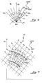
- a region 70 of sector 32 Referring to FIG. 7, a region 70 of sector 32 (FIG.
- the region 70 is generally near a pair of "actual” sonar beams, here beams 307 and 308.
- the region 70 is also near a pair of ranges r i , r (i+1) , as shown.
- forty addition "synthesized beams" shown in FIG. 7 were added by an interpolation process.
- the data points at positions (i, j) associated with the actual beam positions are shown by the symbol (.); here positions P A and P B , (along range r (i+1) ) and positions P C and P D (along range r i ).
- the interpolated data is represented by the symbol (x); here positions P E , P F , P G , P H , P r (along range r (i+1) ), and positions P J , P K , P L , P M , and P N (along range r i ).
- the polar coordinate positions of the normalized energy E'(r i , ⁇ k ) for both the actual and "synthesized" beams are converted to Cartesian coordinate positions.
- the Cartesian coordinates is referenced to the bow of ship 10 and here has its Y-axis aligned in the North direction and its X-axis aligned in the East direction.
- a rectangular Cartesian coordinate grid is shown in FIG. 7 superimposed on the polar plotted position points P A to P N , range line along ranges r i , r (i+1) , and the beams 307 and 308.
- the grid has East/West grid lines E1 to E4, as shown, and North/South grid lines N1 - N4, as shown.
- the North/South grid lines N1 - N4 and East/West grid lines E1 - E4 define an N x M matrix of row and columns of cells C m,n .
- N and M are each 64.
- the grid is square having 64 columns of North/South grid lines and 64 rows of East/West grid lines.
- Each cell C m,n is the region bounded by a pair of successive row grid lines and a pair of successive column grid lines.
- each cell C m,n is square in shape, here having a length ⁇ and a width ⁇ .
- FIG. 7 shows cells C1 - C5 between North/South grid lines N1 - N6 and East/West grid lines E2, E3, for example.
- the global position of the grid lines, N1 - N6, E1 - E4 (and hence the global position of the cells, C m,n ) is known since the global position of ship 10 is known from the global positioning system 44 (FIG. 2).
- FIG. 2 shows an exemplary one of the cells C1 - C4, here cell C2
- it is first noted that such cell C2 is bounded by the pair of North/South grid lines N2, N3 and the pair of East/West grid lines E2, E3, as shown .
- the grid lines N2, and N3 are at x-axis (i.e. East/West) positions x (m- ⁇ /2) , x (m+ ⁇ /2) , respectively and the grid lines E2, E3 are at y-axis (i.e. North/South) positions y (n- ⁇ /2) , y (n+ ⁇ /2) , respectively.
- cell C2, i.e. C m,n)
- the processor 42 in response to instructions stored in the program memory 40, stores the calculated x,y position for all 3,724 normalized energy data, E'(r i , ⁇ k ), and stores the results in a memory section, not shown, of the data memory 44. Thus, for each normalized energy data E'(r i , ⁇ k ), the x,y position thereof is stored in such memory section.
- the processor 42 in response to stored instructions, reads such memory section and determines which one of the 4,096 cells C m,n , includes such x,y position.
- the processor 42 also counts the number, N m,n of normalized energy data points (i.e. samples) in each one of the cells (i.e.
- N m,n is the number of samples in cell C m,n ).
- N m,n 2 samples
- the 3,724 normalized energy samples, E' ⁇ (x m ,y n ) and the number of samples, N m,n in each of the 4,096 cells, C m,n, , are stored as data in normalized global position energy memory section 72.
- processor 42 in response to instructions stored in program memory 40, reads the 3,724 normalized energy samples, E' ⁇ (x m ,y n ) and the number of samples, N m,n in each of the 4,096 cells, C m,n, , from the normalized global position energy memory section 72. From such read data the processor 42 computes, for each of the 4,096 cell, C m,n , a statistically space and time averaged slope detection characteristic, Y m,n .
- the slope detection statistic,Y m,n is calculated in accordance with the following equation: From the equation above it is first observed that the normalized energy samples, E' ⁇ (x m ,y n ), represent the sonar energy level normalized by the estimated energy level for a flat sea bottom. Thus, if the level of the normalized energy sample, E' ⁇ (x m ,y n ) is one (i.e. 1) from the equation above
- the parameter a varies linearly with the speed of ship 10.
- Processor 42 in response to instructions stored in the program memory 40, reads the average slope detection statistic, Y ⁇ m,n (g), from memory section 76 and determines, for each cell C(m,n), whether the sonar has detected a statistically significant slope in such cell C(m,n) of concern to the safety of the ship. More particularly, the average slope detection statistic [ Y ⁇ m,n (g) ] is compared with a threshold level, TH. A typical default threshold level is 1; however, the threshold level can be operator selected.
- FIG. 8 shows a portion of the 4,096 cells, here a six by six cell array portion (i.e. cells C m,n to C (m+5,n+5) ).
- the detection signals S m,n to S (m+5,n+5) are here indicated as 0 except for the following cells where the detection signals are indicated as 1: C m,n ; C m,(n+1) ; C (m+1),n ; C (m+2),n ; C (m+3),n ; C (m+4),n ; C (m+2),(n+2) ; C (m+2),(n+4) ; C (m+3),(n+2) ; C (m+3),(n+3) ; C (m+4),(n+2) ; and, C (m+4),(n+4) , as shown.
- the processor 42 in response to instructions stored in program memory 40 and data read from the detection signal [S m,n ] memory section 78, associates detected cell slopes into clusters, or regions, R j .
- clusters or regions, R j .
- Region R1 is made up of cells: C m,n ; C m,(n+1) ; C (m+1),n ; C (m+1),n ; C (m+3),n ; and, C (m+4),n and region R2 is made up of cells: C (m+2),(n+2) ; C (m+2),(n+4) ; C (m+3),(n+2) ; C (m+3),(n+3) ; C (m+4),(n+2) ; and, C (m+4),(n+4) .
- the regions, R j are stored in the sonar data slope memory section 49, as shown in FIGs 3B and 9. Thus each region, R j , is indexed and the Cartesian coordinate positions of the regions are stored, as indicated.
- the processor 42 examines in sequence each of the cells C m,n to C (m+5),(n+5) on a row by row basis.
- the process starts with the cell in the lower left hand corner (i.e. Cell (m+5),n ) and continues from left to right (i.e. to Cell (m+5),(n+5) ), then progresses upward to the next higher row, to Cell (m+4),n , and continues, on a row by row basis, until Cell m,(n+5) , in this example, is examined.
- the examination process is summarized by the flow diagram in FIG 8A and is as follows: If the sonar energy slope.
- the cells to the left, bottom left, bottom, and bottom right of the C (m+3),(n+3) are: C (m+3),(n+2) , C (m+4),(n+2) , C (m+4),(n+3) , C (m+4),(n+4) , respectively).
- the ID#s of the cells of the "neighboring" cells are "looked at” in the following sequence: first the cell to the left of the examined cell is “looked at”, next the cell to the bottom of the examined cell is “looked at”, next the cell to the bottom left of the examined cell is “looked at”, and finally the cell to the bottom right of the examined cell is “looked at”. If none of the "neighboring" cell to the cell being examined have a non-zero ID#, the cell being examined is given the next successive, non-zero ID#.
- the cell under examination is assigned the ID# of first non-zero ID# in the sequence of "neighboring" cells "looked at” (i.e. the sequence of: left, bottom, bottom left, and finally the bottom right of the examined cell, as discussed above). If the ID# assigned to the cell under examination is the same as the ID# of all cells "neighboring" cell being "looked at”, the processor 42 examines the next cell in the process. If, however, a sequentially "looked at", "neighboring" cell, has an ID# different from the ID# assigned to the cell under examination, then each previously examined cell having this different ID# is reassigned the ID# of the cell being examined.
- a zero ID# is assigned for cells C (m+5,n) , C (m+5,n+1) , C (m+5,n+2) , C (m+5,n+3) , C (m+5,n+4) , C (m+5,n+5) , as shown in FIG. 8B, because none of these cells had a level that crossed the threshold level, TH.
- the next cell examined (FIG. 8) is cell C (m+4),n . This cell had a level that did cross the threshold level. Further there are no cells to the left, bottom left, bottom or bottom right of the examined cell that has been assigned a non-zero ID#.
- the examined cell, C (m+4),n is assigned the next consecutive ID#, here ID#1, as shown in FIG. 8B.
- the next cell examined (FIG. 8), C (m+4),(n+1) did not cross the threshold TH and therefore is assigned a zero ID#, as shown in FIG. 8B.
- the next examined cell (FIG. 8), cell C (m+4),(n+2) has a level that crossed the threshold level. None of the cells to the left, bottom left, bottom, or bottom right to the examined cell has been assigned a non-zero ID#. Therefore the examined cell, here cell C (m+4),(n+2) , is assigned the next consecutive non-zero ID#, here ID#2, as shown in FIG. 8B.
- the next examined cell is cell C (m+4),(n+3) . This cell did not cross the threshold level and therefore it is assigned a zero ID#, as shown in FIG. 8B.
- the next cell examined is cell C (m+4),(n+4) . This cell had a level that crossed the threshold level. None of the cells to the left, bottom left, bottom, or bottom right of the examined cell has been assigned a non-zero ID#. Therefore cell C (m+4),(n+4) , is assigned the next consecutive non-zero ID#. Thus, cell C (m+4),(n+4) is assigned ID#3, as shown in FIG. 8B.
- the next examined cell is cell C (m+4),(n+5) . This cell did not cross the threshold level and therefore it is assigned a zero ID#, as shown in FIG. 8B.
- cell C (m+3),n The next cell examined (FIG. 8) is cell C (m+3),n .
- This cell had a level that crossed the threshold level. Only one of the cells to the left, bottom left, bottom, or bottom right of the examined cell, here the cell to the bottom of the examined cell (i.e. cell C (m+4),n has been assigned a non-zero ID#, here ID#1. Therefore cell C (m+3),n , is assigned the same non-zero ID# as cell C (m+4),n . Thus, examined cell C (m+3),n assigned ID#1, as shown in FIG. 8B.
- cell C (m+3),(n+3) is examined, the processor 42 "looks at" the "neighboring" cells in the sequence discussed above.
- the first "neighboring" cell looked at” is cell C (m+3),(n+2) , which here has an ID#2.
- cell C (m+3),(n+3) is assigned ID#2.
- the next cell in the sequence "looked at” is cell C (m+4),(n+2) , which has the same ID# as that assigned to cell C (m+3),(n+3) , i.e. ID#2.
- the next cell in the sequence "looked at” is cell C (m+4),(n+3) ; however this cell has a zero ID# so that the processor 42 skips this zero ID# cell and "looks at” the next, "neighboring" cell in the sequence, here cell C (m+4),(n+4) .
- Cell C (m+4),(n+4) was previously assigned an ID# of ID#3.
- the ID# assigned to "neighboring" cell C (m+4),(n+4) is different from the ID# of the cell, C (m+3),(n+3) currently being examined.
- the processor 42 reassigns all cells having the ID# of the "looked at", "neighboring" cell C (m+4),(n+4) (i.e. the ID#3) to the ID# of the cell being examined (i.e. the ID# of the cell C (m+3),(n+3) ), as shown.
- the processor 42 continues, as discussed, to assign the cells ID#'s, as shown for the example in FIG. 8C.
- processor 42 groups all cells having the same ID#'s into a common region, R(j), as discussed above in connection with FIG. 9.
- R(j) a common region
- Region R1 is made up of cells: C m,n ; C m,(n+1) ; C (m+1),n ; C (m+2),n ; C (m+3),n ; and, C (m+4),n (because all these cells have a common ID#, here all have an ID#1) and region R2 is made up of cells: C (m+2),n+2) ; C (m+2),(n+4) ; C (m+3),(n+2) ; C (m+3),(n+3) ; C (m+4),(n+2) ; and, C (m+4),(n+4) (because all these cells have a common ID#, here all have an ID#2).
- Processor 42 in response to instructions stored in the program memory 40, charted depth data stored in charted depth data memory 50, the ship 10 global position (X, Y) obtained from the global position system 44 and the ship 10 heading, ⁇ , relative to North, calculates the slope profile of the sea bottom in front of the ship 10. (It is noted that the slope profile is in the same, Earth, or global, position coordinates as the sonar data slope profile stored in the sonar data slope memory section 49).
- FIG. 10A a chart, of the of the area where the ship is presently located and called up from the charted depth data base memory 50, is shown.
- the chart shows depth contour lines, here a pair of contour lines C1 and C2 as well as depth soundings, here seven depth soundings D1 - D7.
- the data representing these contours lines C1, C2 is stored in the data base memory 50 as X,Y positions having the same depth. More particularly, all positions on line C1 have the same depth and all positions on line C2 have the same depth, but the depth of positions on line C1 is different from the depth of positions on line C2.
- data from contour lines are stored with an index indicating the data is from a contour line.
- Each sounding data, D1 - D7 is stored as a X,Y position, a depth, and an index indicating the data is from a sounding.
- the processor 50 in response to instructions stored in the program memory 40 stores the contour data and the sounding data, together with their contour/sounding index, in a random access memory (RAM), not shown, but which is here a section of the data memory.
- the RAM is adapted to stored 1,000 x 1,000 positions of pixels of data; however in the example shown in FIG. 10A a 22 by 16 array of pixels is shown.
- the contour lines C1 and C2 together with sounding D1 - D7 are shown superimposed on the array of pixels.
- the processor 42 reads the data stored in the pixels on a row by row basis until a pixel storing sounding data (as distinguished from contour data) is detected.
- the first sounding pixel meeting this criteria is the data at sounding D1.
- the processor 42 selects this pixel for further examination.
- the processor 42 determines whether there is any data, from either a neighboring sounding or contour, within a square, eleven by eleven pixel window, W, centered at the pixel under examination. If there are no pixels with data within the window, the process goes to the next sounding. If, on the other hand, there is data within the window, the processor 42 continues to do further processing with the selected pixel.
- the processor 42 identifies the nearest pixel (or pixels if more that one pixel are equidistant from the pixel under examination). The processor 42 then interpolates between the depth of the pixel under examination and the depth of the neighboring pixel and fills with the interpolated data the empty pixels intersected by a line passing between the pixel under examination and the neighboring pixel. If there is data in any pixel intersected by the line, the data in such pixel is not changed.
- an eleven by eleven window, W1 is placed around the first selected cell, here the cell having the sounding D1.
- the window is truncated, as shown along the top boundary.
- contour C1 i.e. data in pixels P1, P2 and P3
- contour C2 i.e. data in pixels P4 - P10
- pixels P1 and P5 are equidistant from sounding D1.
- processor 42 interpolates between the depth at pixel D1 and the depth at pixel P1 to thereby fill-in depth data into pixel disposed along (i.e. intersected by) a line L1 between the two pixels D1 and P1 (i.e. pixels F1, F2, F3) and also interpolates along line L2 to fill-in depth data into pixels intersected by line L2 (i.e. pixels F4 and F5).
- the processor 42 then continues to scan row by row until another sounding is detected, here sounding D2 (see also FIG. 10B). Again the selected sounding D2.
- An eleven by eleven pixel window, W2 is placed around the selected pixel, here the pixel having the sounding D2.
- the window W2 encloses pixels having data are those associated with contour C1, sounding D3, and pixels F1 - F5 which have interpolated data.
- Two of the pixels, here pixels P11 and P12 are closet to the selected pixel D2. (Here the two pixels P11 and P12 are equidistant from the selected pixel D2).
- pixels intersected by lines L3 and L4 i.e. pixels F6 - F9 are filled in with interpolated data.
- the distance from the pixel having sounding D2 to the pixel having sounding D3 is greater than the distance between sounding D2 and the pixels P11 and P12 and thus is not a "nearest neighbor" to be included in the interpolation process.
- the process continues until all sounding in the chart have been selected. After the first pass through, the chart fills in pixels intersected by lines L1 - L9, as shown in FIG. 10C.
- the processor 42 After having selected all soundings, the processor 42 makes a second pass through the chart and again selects the first sounding, here sounding D1. Now, however, the window is increased in size to a thirteen by thirteen pixel window. This process continues until the second pass is completed. The process here fills data into pixels along lines L9, L10, L11 and L12, as shown in FIG. 10D. If the second pass increases the number of previously un-filled pixels by more than two percent, a third pass is made. The process continues and subsequent passes are made through the chart until there is less then a two percent increase in the number of unfilled pixels being filled with interpolated data. When there is less then a two percent increase the second, " rectangular interpolation" is used to complete the interpolation process.
- FIG. 10E shows the lines added as a result of the "nearest neighbor" interpolation process, for purposes of illustration.
- the processor 42 scans the stored data row by row, as before. Now, however, the memory also has data interpolated from the "nearest neighbor” process.
- the processor 42 detects a filled pixel, here whether the pixel has data from a sounding, or the contour, or from interpolated data, a ten pixel window is searched along a row of the detected cell, beginning at the next pixel after the detected cell.
- the processor 42 examines all cells in the same row as the detected cell and fills in all the cells therebetween with interpolated data. After the chart is searched row by row, it is then searched column by column.
- a ten pixel window is searched along a column of the detected cell, beginning at the next pixel after the detected cell.
- the processor 42 examines all cells in the same column as the detected cell and fills in all the cells therebetween with interpolated data.
- the window length is increased from a five pixel length to a ten pixel length. The process is successively repeated with window lengths of 20, 50 and 100. The process continues until the window reaches the boundary of the chart.
- the interpolated charted depth data of the portion of the sea bottom in front of the ship (i.e. in sector 32, FIG. 1) is shown for as an array of rows and columns of cells C 1,1 to C (6,6) as depths D 1,1 to D 6,6 , respectively, as shown.
- the columns of the cells are in the North/South direction and the rows of the cells are in the East/West direction. (This is the same as the rows and columns of cells shown in FIG. 7 for the sonar data produced slopes).
- Each computed slope vector, (m,n) is stored as a complex number in a charted data slope vector memory section 80 (FIG. 3B). Here the data stored in memory section 80 is computed and stored prior to the voyage of ship 10.
- the processor 42 in response to the instructions stored in the program memory 40 and the slope vector data stored in the charted data slope vector memory section 80, calculates the charted data based slope in the direction of the one of the 49 sonar beams, 30 k , where k is an integer from 1 to 49 (i.e. beams 301 - 309 as well as the forty "synthesized" beams).
- k is an integer from 1 to 49 (i.e. beams 301 - 309 as well as the forty "synthesized" beams).
- beam 30 k is shown to pass through such cell C 3,4 .
- beam 30 k is at an angle ⁇ k from the bow line 36 (FIG. 1) of ship 10. Further, ship 10 has a heading of ⁇ from North, as shown.
- the North/South components, s NS (3,4), of the slope vector (3,4) and the East/West components s EW (m,n) of such vector (3,4) are shown, along with the resultant slope vector, (3,4).
- the angle between the slope vector, (3,4), and the beam 30 k is ⁇ . If the direction of the beam 30 k is defined by the unit vector , the portion of the slope vector slope, (m,n) as "seem” by beam 30 k , but produced by the chart (i.e. the slope S CHART ) is equal to: [ ⁇ (m,n); that is, the dot product of and (m,n).
- the slope S CHART is therefore the projection of the resultant slope vector, (m,n), onto the direction of the beam 30 k .
- the slope S CHART for each of the 64 x 64 cells (m,n) is stored in a charted data slope memory section 52 of the data memory 44 (FIG. 3B) at the address location of the cell corresponding thereto.
- the processor 42 in response to instructions stored in the program memory 40, determines whether there is an anomaly. That is, for each cluster, or region, R j , stored in the sonar data slope memory section 49, the processor 42 uses the cells in the cluster as an address for the charted data slope memory section 52 to read the chart slope data S CHART in the addressed cluster.
- the processor 42 determines whether any read chart slope data S CHART contained in any cell in the addressed cluster has a level greater than a S CHART slope threshold, ST, here a slope of 0.5. If so, the cluster and the chart data are consistent and the chart data is considered reliable. On the other hand, if the chart data does not indicate a slope, s CHART , greater than the S CHART slope threshold, ST, here 0.5, there is an anomaly between the chart data and the sonar data. Thus, there may be an underwater hazard detected by the sonar that is not on the chart.
- One possible explanation for the anomaly is the presence of a surface ship. That kind of anomaly is resolved by the ship radar.
- Information produced by the computer is fed to display 51 (FIG.1), as shown in FIG. 12.
- An anomaly is indicated by a circle, 90, as shown.
- the circle 90 can be displayed in a different color than the regions R j , for example, and /or may be displayed in a "blinking" format.
Abstract
Description
- This invention relates generally to sonar systems and more particularly to sonar systems adapted to aid in the detection and avoidance of sea bottom hazards which could damage a sea going vessel's hull.
- As is known in the art, charted depth data is used as a primary navigation aid in avoiding reef and other sea bottom hazards. Sometimes this charted depth information changes over time because earth disturbances may create new, previously uncharted hazards. Thus, current underwater hazard avoidance techniques are supplemented with on-board sonar mapping of the sea's bottom. Current sonar imaging provides high resolution of the sea bottom profile when using a vertical, or substantially vertical, depth measurement. However, with the advent of large ocean-going vessels, particularly the new massive oil tankers, early warning of forward navigational hazards is required because of the relatively long intervals of time which are required either to slow down or to change course.
- In accordance with the present invention a system for providing advance warning of underwater navigation hazards that threaten safe ship passage is provided. The system includes a sonar transmitter/receiver adapted for mounting on the ship in a forward looking direction. A processor, in response to sonar returns produced by the sonar transmitter/receiver, produces a sonar produced slope profile of a region of the sea bottom in front of the path of the vessel. A charted data produced slope profile is developed from charted depth data. The charted depth data developed slope profile is compared with the sonar return produced slope profile to determine whether the sonar produced slope profile and the charted depth data slope profile are consistent with each other. If the sonar return produced slope profile in a region of the sea bottom is greater that a predetermined threshold level (selected to identify a potential forward undersea hazard) and, if the charted depth data generated profile of such region does not indicate this potential hazard, an anomaly is identified and a signal indicating such anomaly is produced.
- In a preferred embodiment of the invention, the system estimates the energy in sonar returns from a sea having a substantially flat bottom. The energy in sonar returns are then normalized by the estimated flat sea bottom energy to enhance the identification of hazardous high slope sea bottom profile regions.
- For a more complete understanding of the concepts of the invention reference is now made to the following drawings, in which:
- FIG. 1 is a sketch illustrating a ship navigating through a body of water using an anti-collision system according to the invention;
- FIG. 2 is a block diagram of the anti-collision system used by the ship in FIG. 1;
- FIG. 3 is a diagram showing the relationship between FIGs. 3A and 3B, FIGs. 3A and 3B being, together, a block diagram of a digital computer used in the anti-collision system of FIG. 2;
- FIG. 4 is a diagram showing the angular direction of beams formed by a sonar system used in the anti-collision system of FIG. 2;
- FIG. 5 is block diagram of an estimator used by the anti-collision system of FIG. 2 to estimate the flat profile of the sea bottom;
- FIG. 6 is a curve representing an equation of the estimated energy of a received sonar signal from reverberations from a flat sea bottom, such equation being used by the estimator of FIG. 5;
- FIG. 7 is a diagram showing a portion of the beams of FIG. 4 produced by the sonar system relative to North;
- FIG. 8 is a diagram showing an example of sonar produced sea bottom slopes after processing by a threshold level detection process, such slopes being shown for a number of cell positions of the sea bottom, such diagram being useful in understanding a cluster, or region, identification process used to identify regions of the sea bottom having relatively large slopes;
- FIG. 8A is a flow diagram useful in understanding the cluster, or region, identification process of FIG. 8;
- FIGs. 8B and 8C are diagrams useful in understanding the cluster, or region, identification process of FIG. 8;
- FIG. 9 is a chart showing the cells of FIG. 8 in various regions identified by the process described in connection with FIGs. 8, 8A, 8B and 8C;
- FIGs. 10A to 10E are charts useful in understanding n interpolation process used to generate depth information for determining sea bottom slope information from charted depth information;
- FIG. 11 is a diagram showing the relationship between a sea bottom slope vector, produced from the charted sea bottom information discussed in connection with FIGs. 11A to 11E, and the direction of a beam produced by the sonar system and discussed in connection with FIG. 7; and,
- FIG. 12 is an exemplary view of a display used in the system of FIG. 1.
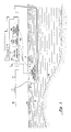
- Referring now to FIG. 1, a
ship 10 is shown navigating through a body ofwater 12. Theship 10 carries on board ananti-collision sonar system 14. Thesystem 14 provides advance warning of underwater navigation hazards that threaten safe passage forship 10, particularly hazards in shallow water (i.e., between 10 - 20 fathoms). Thesystem 14 includes a sonar transmitter/receiver section 16 mounted in a forward position ofship 10, as shown. Referring also to FIG. 2, the transmitter/receiver section 16 includes anarray 18, here a cylindrical array of conventional transmitting/receiving transducers mounted in thehull section 19 of ship 10 a sufficient distance below the surface 22 (FIG. 1) of the body ofwater 12 so that high level sonar pressures can be produced without cavitation. Thus, the sonar transmitter/receiver 16 is adapted for mounting on a sea going vessel, hereship 10, in a forward looking direction 21 (FIG.1). Thesystem 10 includes adigital computer 24 for sending ping trigger pulses, vialine 25, to a conventional sonar transmitter waveform and (inverse)beamforming computer 20. Digital signals produced bycomputer 20 are converted into analog signals by analog to digital converters (not shown), such converted analog signals being amplified by power amplifiers (not shown), such amplified signals being fed to a transmit/receiveswitching network 23, in a conventional manner. In response to each ping trigger signal the transmitter waveform and (inverse)beamforming computer 20 transmits an electrical pulse online 21 initially places the transit/receive (T/R)switching network 23 in a transmit mode. Thus, as is well known, in the transmit mode, the output of the transmitter and waveform (inverse)beamforming computer 20 is coupled to thearray 18 of transmitting/receivingtransducers 18 so that a ping of sonar energy introduced into the body ofwater 12. Subsequently, the signal online 21 changes, and the T/R switching network 23 is placed in the receive mode. Thus, as is well known, in the receive mode thearray 18 of transmitting/receiving transducers is coupled to a conventional receivingbeam forming network 29 throughamplifiers 26 and analog to digital converters (A/D) 27. Thereceiving beamforming network 29 produces, in a conventional manner, a plurality of, here nine for example, simultaneously existing receiving beams 30₁ - 30₉ arranged to cover a ninetydegree sector 32 in front of the ship 10 (i.e., forty-five degrees on either side of bow line 36). (It should be understood that a larger number of beams than 9 beams, for example 12 beams may be preferable in which case a planar array of transducers may be used). Thus, each one of the beams 30₁ - 30₉ has a different angular direction. Here, the centerlines of the nine beams 30₁ - 30₉ have angular deviations from thebow line 36 ofship 10 of: ϑ₁ = -40 degrees; ϑ₂ = -30 degrees; ϑ₃ = -20 degrees; ϑ₄ = -10 degrees; ϑ₅ = zero degrees; ϑ₆ = +10 degrees; ϑ₇ = +20 degrees; ϑ₈ = +30 degrees; and, ϑ₉ = +40 degrees, respectively. The horizontal beam width of each beam is here 10 degrees (i.e. ± 5 degrees about the beam centerline). The centerlines of the beams 30₁ - 30₉ are substantially parallel with the surface of the body of water. The transmitted acoustic power is here in the order of 10,000 watts. - The digital computer 24 (FIG. 2) includes a program or
instruction memory 40, aprocessor 42 and adata memory 44, all arranged in a conventional manner. Here thedigital computer 24 is a Silicon Graphics workstation, Model 4D-35. Theprogram memory 40 stores a set of computer instruction for execution by theprocessor 42 in a manner to be described. Theprocessor 42, in response to the instructions, processes data stored in one, or more memory sections of thedata memory 44 and stores processed data in one, or more, other memory sections of thedata memory 44 in a manner to be described in detail hereinafter. (It should be noted that not all sections of thedata memory 44 have been given a numerical designation, it being understood that sufficient memory is available in thedata memory 44 for theprocessor 42 to perform various required computations, comparisons and processing described herein). Suffice it to say here, however, that theprocessor 42, in response to sonar returns produced by the sonar transmitter/receiver 16, global position information (X, Y) ofship 10 supplied by a global positioning system (GPS) 45,ship 10 heading information relative to North, β, provided by the ship'sgyro compass 46 and the instructions stored inprogram memory 40, calculates a sonar generated data (i.e., echo return generated data) profile of the slope of the sea bottom 48 (FIG. 1) in thesector 32 in front of the path of theship 10. (i.e. thesector 32 covered by the receiving beams 30₁ - 30₉). That is, theprocessor 42 produces a sonar data generated slope profile of a region of the sea bottom 48 in front of the path of the ship based on the sonar return data. This sonar produced slope data is stored in sonar dataslope memory section 49 ofdata memory 44, in a manner to be described. Suffice it to say here, however, that clusters, or regions, insector 32 are identified as having relatively large, hazard potential, slope profiles. - A charted
depth memory 50 is provided for storing charted sea bottom depth information as a function of the global position (X,Y) of theship 10. The charted depth data information is loaded in the charteddepth memory 50 prior to theship 10's voyage. Such data base is generated by converting paper charts available from the National Oceanographic and Atmospheric Administration (N.O.A.A.) or the Defense Mapping Agency (D.M.A.) into digital information in a form to be described hereinafter. Suffice it to say here, however, that, in response to the global position (i.e., X,Y) of the ship, such information being provided by theglobal positioning system 50, charted depth information of thesector 32 in front ofship 10 is read from charteddepth memory 50 by theprocessor 42. In response to this read charted depth information, and the heading, β, of theship 10, theprocessor 42 calculates a charted depth data generated slope profile of the sea bottom 48 (FIG. 1) in thesector 32. That is, a slope profile of thesector 32 of the sea bottom 48 in front of theship 10 based on charted depth data. Such computed, charted depth data generated slope profile is stored inmemory section 52 of thedata memory 44. - The
processor 42, in response to instructions stored in theprogram memory 40 correlates, or compares, the stored charted data generated slope profile information with the sonar generated slope profile information stored in the sonar dataslope memory section 49 to determine whether the latter slope profile is consistent with the former slope profile. If they are not correlated (i.e., consistent one with the other), an anomaly is identified andship 10 must proceed with caution. Information produced by thecomputer 24 is fed to adisplay 51. - More particularly, in response to each sonar ping transmitted, an echo return is received and converted into electrical signals by
array 18 in a conventional manner. The electrical signals pass through the T/R switching network 23,amplifiers 26, A/D converters 27 are combined, in a conventional manner, by the receivingbeam forming computer 29 to produce digital words on lines 54₁ - 54₉. As is well known, then, the envelope of the digitized signals on lines 54₁ - 54₉, respectively, represent the intensities, I(r, ϑ₁) - I(r,ϑ₉), of the sonar returns received by beams 30₁ - 30₉, respectively, as a function of range, r, measured from thebow 19 ofship 10. Thus, for each one of the nine beams, 30₁ - 30₉, nine series of digital words are produced. Each one of the digital words in each of the series represents the intensity of the echo return signal at a corresponding range, r, from thebow 19 ofship 10. Here, 76 range samples, corresponding to ranges r₁ to r₇₆, for each one of the beams 30₁ - 30₉. The series of digital words I(r₁,ϑ₁) - I(r₇₆,ϑ₁) online 56₁ through the series of digital words I(r₁,ϑ₉) - I(r₇₆,ϑ₉) online 56₉, respectively, are fed to thedata memory 44, as shown. - Referring now to FIGs. 3, 3A, and 3B, the
digital computer 24 is shown. The series of digital words on each of lines 56₁ - 56₉ are fed to a position intensity memory section 60 ofdata memory 44. In response to the instructions stored in theprogram memory 40,processor 42 produces control signals to enable the digital words on line 56₁ - 56₉ to become stored in position intensity memory section 60. Thus, memory section 60 may be considered as having a matrix of memory locations, here a matrix of nine column (i.e., one column for each one of the beams 30₁ - 30₉) and 76 rows (i.e., one row for each of the 76 range samples). The intensity data stored in a typical position (i,j) in sector 32 (FIG. 2) is therefore, as shown in FIG. 4, I(ri,ϑj), where, here, i is an integer from 1 to 76 and j is an integer from 1 to 9. - The intensity data I(ri,ϑj) stored in memory section 60 is next read therefrom by
processor 42 in response to instructions stored in theprogram memory 40. Theprocessor 42 then computes the energy E(ri,ϑj) in each position (i,j) by integrating over time, t, over the pulse length, τ, in accordance with: E(ri,ϑj) = ∫| I(ri,ϑj)|² dt. The calculated energy, E(ri,ϑj) for each of the, here 9 x 76 = 684 range - beams positions, is stored in a corresponding one of 684 memory locations of position energy memory section 62 ofdata memory 44. - In order to enhance echo returns from sea bottom slopes, it is desirable to normalize out of the total sonar return the contribution expected from a sea having a substantially flat bottom. To provide this normalization a mathematical model, or equation, is assumed to characterize flat bottom returns (i.e. reverberations) in "shallow" water. "Shallow" water is defined in the underwater acoustics context, where sound propagation encounters numerous interactions with the sea bottom. In the large ship context "shallow" water is defined as charted water depths from 10 to 20 fathoms.
- More particularly, sonar echo returns, in the general case, are made up of both current sea bottom reverberations and non-sea bottom reverberations. The energy in the echo return may be expressed as:

where: r is range; r O is the transition range from the source necessary for distributed backscattering; IT(r O ) is the transmitted sound intensity at r O ; n is an integer selected to match the total two way spreading loss (n = 2 for cylindrical spreading); α is the attenuation factor resulting from forward scattering losses at the boundaries and absorption loss in the water column; φ is the horizontal beamwidth; Δz(r)/Δr is the slope of the vertical discontinuity over Δr at r; Sbd is the backscattering strength of the bottom discontinuity; Sbf is the backscattering strength of the flat bottom; Δr = cτ/2 is the processing range resolution; c is the speed of sound; τ is the active signal pulse length; and N is the system noise floor. - A re-expression of the flat sea bottom portion of the return is made, to facilitate in a least root mean square estimation process to be described hereinafter, Suffice it to say here, however, that such re-expression is:

where, referring also to FIG. 6 (which is a plot of the equation above) : - k
- = the first received energy value of the sonar returns;
- r̂O
- = the range break;
- r̂d
- = the range of the day, which is the maximum range of the sonar for the sea conditions of the day;
- α̂
- = the exponential change in energy with range between r̂O and d (generally referred to as the absorption loss coefficient).
- Thus, the expected flat bottom reverberation energy, Ê(ri,ϑj), for each position (i,j) is computed by first estimating: the first received energy value of the sonar returns, k; r̂O = the range break; r̂d = the range of the day; α̂ = the change in energy with range between r̂O and r̂d. That is, referring also to FIG. 5, in response to each sonar ping, the sonar detected energy E(i,j) for each position (i,j) is subtracted from an estimated energy, ÊR(ri,ϑj), for the corresponding position (i,j) and the difference, ε(ri,ϑj), for each position (i,j) is evaluated. The parameters r̂O, r̂d, and α̂ are adjusted to minimize the root mean square error (RMS) ε(ri,ϑj) for each position (i,j), using conventional (RMS) estimation processing techniques. Thus, there is produced, in response to each ping, one set of parameters for each one of the beams 30₁ - 30₉. ping. While additional memory sections in the
data memory 44 would be used in the estimation processing, such memory sections are not shown. In any event, the estimate, ÊR(ri,ϑj), of flat bottom "shallow" water reverberation in the region in front of ship 10 (i.e.sector 32, FIG. 2) for each of the 9 x 76 positions (i,j) is stored in a corresponding memory location of a flat bottom reverberation memory section 64 (FIG. 3A). Next theprocessor 42, in response to instructions in theprogram memory 40, reads the sonar return energy E(ri,ϑj) stored in the position energy memory section 62 and the estimated flat bottom reverberation energy, ÊR(ri,ϑj) data stored in the flat bottom reverberationenergy memory section 64. In response to such read data, theprocessor 42 normalizes sonar energy data, E(ri,ϑj) stored in memory 62 by the estimated flat bottom reverberation energy ÊR(ri,ϑj) stored inmemory 64, to produce, for each position (i,j) a normalized energy, E'R(ri,ϑj), accordance with:
The normalized energy E'(ri,ϑj) for each position (i,j) is stored in a normalized energyposition memory section 66. -
Next processor 42, in response to the instructions stored in theprogram memory 40, reads the normalized energy data, E'(ri,ϑj), from the normalizedenergy memory section 66 and increases the number of beam data points from nine to, here, forty-nine, using a conventional interpolation process. That is, the normalized energy E'(ri,ϑj) is subtracted from the normalized energy, E'(ri,ϑ(j+1)) (i.e. energy at the same range,ri, but at an adjacent beam angle, ϑ(j+1). The difference,Δ, in energy (i.e. Δ = E'(ri,ϑj) - E'(ri,ϑ(j+1)) is divided by five and appropriately distributed to pixel positions at the same range ri, but at five "synthesized beam" positions having angular positions between the angle ϑj and ϑ(j+1). Thus, instead of having data for only nine beam positions (i.e. at angle of -40,-30,-20,-10,0,+10,+20,+30,+40 degrees, as discussed above), data is generated by the interpolation process for forty additional "synthesized beam positions" (i.e. approximately -38.3, -36.7, -35, -33.4, -31.7, -28.3...+38.3 degrees). Thus there are now pixels at positions (i,k) where k is an integer from 1 to 49. The interpolated energy E'(ri,ϑk) for each of the forty nine beam positions,ϑk, is stored in an interpolated normalizedenergy memory section 68. - As noted from the discussion above, the interpolated energy data, E'(ri,ϑk), stored in
memory section 68 is in polar (i.e. r,ϑ) coordinates. Theprocessor 42, in response to instructions stored in theprogram memory 40, the global position, X,Y ofship 10, and the bearing, β, ofship 10 relative to north, N, (FIG. 4), converts the energy data, E(ri,ϑk), into Cartesian coordinates (i.e. into E'(xm,yn)). Here there are 64 x 64 cells (i.e. m is an integer from 1 to 64 and n is an integer from 1 to 64). Referring to FIG. 7, aregion 70 of sector 32 (FIG. 4) is enlarged. Theregion 70 is generally near a pair of "actual" sonar beams, here beams 30₇ and 30₈. Theregion 70 is also near a pair of ranges ri, r(i+1), as shown. As described above forty addition "synthesized beams" (shown in FIG. 7) were added by an interpolation process. In FIG. 7, the data points at positions (i, j) associated with the actual beam positions are shown by the symbol (.); here positions PA and PB, (along range r(i+1)) and positions PC and PD (along range ri). The interpolated data is represented by the symbol (x); here positions PE, PF, PG, PH, Pr (along range r(i+1)), and positions PJ, PK, PL, PM, and PN (along range ri). The polar coordinate positions of the normalized energy E'(ri,ϑk) for both the actual and "synthesized" beams are converted to Cartesian coordinate positions. The Cartesian coordinates is referenced to the bow ofship 10 and here has its Y-axis aligned in the North direction and its X-axis aligned in the East direction. Thus, the conversion is made by theprocessor 42 in accordance with:

where: xi,k is the position of E'(ri,ϑ) along the North/South direction; yi,k is the position of E'(ri,ϑk) along the East/West direction; and, z is the angle between the beam, at angle ϑk, and North (N). A rectangular Cartesian coordinate grid is shown in FIG. 7 superimposed on the polar plotted position points PA to PN, range line along ranges ri, r(i+1), and thebeams ship 10 is known from the global positioning system 44 (FIG. 2). Thus, considering an exemplary one of the cells C₁ - C₄, here cell C₂, it is first noted that such cell C₂ is bounded by the pair of North/South grid lines N₂, N₃ and the pair of East/West grid lines E₂, E₃, as shown . The grid lines N₂, and N₃ are at x-axis (i.e. East/West) positions x(m-γ/2), x(m+γ/2), respectively and the grid lines E₂, E₃ are at y-axis (i.e. North/South) positions y(n-γ/2), y(n+γ/2), respectively. Thus, cell C₂, (i.e. Cm,n)) is at a position in the Cartesian coordinate system of xm, yn. It is also noted that the number of sonar (actual and "synthesized") data points is here 49 x 76 = 3,724, (i.e. 3,724 polar plotted position points, P) while the number of cells is here 64 x 64 = 4,096. Any one of the cells may have more than one polar plotted position points, P. For example, in FIG. 7, the exemplary cell, Cm,n, (i.e. cell C₂ here has two polar plotted position points, PE and PF. - The
processor 42, in response to instructions stored in theprogram memory 40, stores the calculated x,y position for all 3,724 normalized energy data, E'(ri,ϑk), and stores the results in a memory section, not shown, of thedata memory 44. Thus, for each normalized energy data E'(ri,ϑk), the x,y position thereof is stored in such memory section. Theprocessor 42, in response to stored instructions, reads such memory section and determines which one of the 4,096 cells Cm,n, includes such x,y position. Theprocessor 42 also counts the number, Nm,n of normalized energy data points (i.e. samples) in each one of the cells (i.e. Nm,n is the number of samples in cell Cm,n). Thus, considering the exemplary cell Cm,n (here C₂) shown in FIG. 7, such cell Cm,n (i.e. C₂) has two samples (i.e. Nm,n = 2): E'₁(xm,yn), and E'₂(xm,yn) (i.e. in the general case, E'τ(xm,yn), where τ is the number of the energy samples). The 3,724 normalized energy samples, E'τ(xm,yn) and the number of samples, Nm,n in each of the 4,096 cells, Cm,n,, are stored as data in normalized global positionenergy memory section 72. - Next,
processor 42, in response to instructions stored inprogram memory 40, reads the 3,724 normalized energy samples, E'τ(xm,yn) and the number of samples, Nm,n in each of the 4,096 cells, Cm,n,, from the normalized global positionenergy memory section 72. From such read data theprocessor 42 computes, for each of the 4,096 cell, Cm,n, a statistically space and time averaged slope detection characteristic, Ym,n. The slope detection statistic,Ym,n, is calculated in accordance with the following equation:
From the equation above it is first observed that the normalized energy samples, E'τ(xm,yn), represent the sonar energy level normalized by the estimated energy level for a flat sea bottom. Thus, if the level of the normalized energy sample, E'τ(xm,yn) is one (i.e. 1) from the equation above | E'τ(xm,yn) - 1| will equal 0. Thus, log (1 + | E'τ(xm,yn) - 1| will equal zero indicating the absence of a sea bottom slope (i.e. the presence of a flat sea bottom). Thus, this portion of the equation will increase in level with increasing sea bottom slope. It is next observed that only large slopes are detected because the log function increases in units of one in response to an order of magnitude (i.e. 10:1) change is sea bottom slope. Finally, it is observed that the equation above averages the calculation, log (1 + |E'τ(xm,yn) - 1| , over all, Nm,n energy samples in cell Cm,n. (This process of forming a detection statistic from multiple spatial samples, as represented by the above equation, is sometimes referred to as a log likelihood ratio detector with a zero velocity hypothesis (i.e. stationary, or flat, sea bottom feature)). Theprocessor 42 stores the 4,096 calculated slope detection statistic,Ym,n, in a slope detectionstatistic memory section 74. -
Next processor 42 reads the calculated slope detection statistic, Ym,n, from the slope detectionstatistic memory section 74 and filters (i.e. time averaging) or smooths the statistic, Ym,n, over successive pings. This filtering is performed byprocessor 42 for each of the 4,096 cells Cm,n, in accordance with the following equation:
where: a + b = 1.0 and g is the ping index. The parameter a varies linearly with the speed ofship 10. Here, for example, if the speed ofship 10 is 5 knots, and the range R₇₆ is 10,000 yards and the length of cell Cm,n is 320 yards, a = 0.05 and b = 0.95. The process represented by the equation above may be characterized as low pass filtering using a low pass filter with a time constant of (1/a), here 20. Thus, here it takes 20 pings to build up to a steady state value if a step change were made in the slope detection statistic, Ym,n. The calculated average slope detection statistic,
-
Processor 42, in response to instructions stored in theprogram memory 40, reads the average slope detection statistic,


processor 42 produces a detection signal, Sm,n = 1; on the other hand, if the average slope detection statistic [
processor 42 produces a detection signal, Sm,n = 0. The detection signals Sm,n are stored in a detection signal [Sm,m]memory section 78. FIG. 8 shows a portion of the 4,096 cells, here a six by six cell array portion (i.e. cells Cm,n to C(m+5,n+5)). The detection signals Sm,n to S(m+5,n+5) are here indicated as 0 except for the following cells where the detection signals are indicated as 1: Cm,n; Cm,(n+1); C(m+1),n; C(m+2),n; C(m+3),n; C(m+4),n; C(m+2),(n+2); C(m+2),(n+4); C(m+3),(n+2); C(m+3),(n+3); C(m+4),(n+2); and, C(m+4),(n+4), as shown. - The
processor 42, in response to instructions stored inprogram memory 40 and data read from the detection signal [Sm,n]memory section 78, associates detected cell slopes into clusters, or regions, Rj. Thus, there are in this example two clusters, or regions: R₁ and R₂ (i.e. j = 2) in the sea bottom. Region R₁ is made up of cells: Cm,n; Cm,(n+1); C(m+1),n; C(m+1),n; C(m+3),n; and, C(m+4),n and region R₂ is made up of cells: C(m+2),(n+2); C(m+2),(n+4); C(m+3),(n+2); C(m+3),(n+3); C(m+4),(n+2); and, C(m+4),(n+4).
The regions, Rj, are stored in the sonar dataslope memory section 49, as shown in FIGs 3B and 9. Thus each region, Rj, is indexed and the Cartesian coordinate positions of the regions are stored, as indicated. - More particularly, referring to FIG. 8 the
processor 42 examines in sequence each of the cells Cm,n to C(m+5),(n+5) on a row by row basis. Here, the process starts with the cell in the lower left hand corner (i.e. Cell(m+5),n) and continues from left to right (i.e. to Cell(m+5),(n+5)), then progresses upward to the next higher row, to Cell(m+4),n, and continues, on a row by row basis, until Cellm,(n+5), in this example, is examined. The examination process is summarized by the flow diagram in FIG 8A and is as follows: If the sonar energy slope. Sm,n of the cell being examined did not cross the slope/no slope decision threshold, TH, (i.e. Sn,m = 0) an identification number (ID#) of zero is assigned to the cell. If, on the other hand, the energy slope Sm,n of the cell being examined did have an energy level that crossed the threshold, TH, (i.e. Sm,n = 1) a non-zero ID# is assigned to the cell. More particularly, if the examined cell had a level that crossed the threshold, TH, the ID#s assigned to "neighboring" cells of the examined cell are "looked at". (Here the "neighboring" cells to be "looked at" are the cells to the left, bottom left, bottom or bottom right of the examined cell. Thus, referring to FIG.8, the cells to the left, bottom left, bottom, and bottom right of the C(m+3),(n+3) are: C(m+3),(n+2), C(m+4),(n+2), C(m+4),(n+3), C(m+4),(n+4), respectively). Here, the ID#s of the cells of the "neighboring" cells are "looked at" in the following sequence: first the cell to the left of the examined cell is "looked at", next the cell to the bottom of the examined cell is "looked at", next the cell to the bottom left of the examined cell is "looked at", and finally the cell to the bottom right of the examined cell is "looked at". If none of the "neighboring" cell to the cell being examined have a non-zero ID#, the cell being examined is given the next successive, non-zero ID#. If, however, any of the "neighboring" cells "looked at" has a non-zero ID#, the cell under examination is assigned the ID# of first non-zero ID# in the sequence of "neighboring" cells "looked at" (i.e. the sequence of: left, bottom, bottom left, and finally the bottom right of the examined cell, as discussed above). If the ID# assigned to the cell under examination is the same as the ID# of all cells "neighboring" cell being "looked at", theprocessor 42 examines the next cell in the process. If, however, a sequentially "looked at", "neighboring" cell, has an ID# different from the ID# assigned to the cell under examination, then each previously examined cell having this different ID# is reassigned the ID# of the cell being examined. - Thus, referring to the example shown if FIG. 8, a zero ID# is assigned for cells C(m+5,n), C(m+5,n+1), C(m+5,n+2), C(m+5,n+3), C(m+5,n+4), C(m+5,n+5), as shown in FIG. 8B, because none of these cells had a level that crossed the threshold level, TH. The next cell examined (FIG. 8) is cell C(m+4),n. This cell had a level that did cross the threshold level. Further there are no cells to the left, bottom left, bottom or bottom right of the examined cell that has been assigned a non-zero ID#. Therefore the examined cell, C(m+4),n, is assigned the next consecutive ID#, here
ID# ₁, as shown in FIG. 8B. The next cell examined (FIG. 8), C(m+4),(n+1), did not cross the threshold TH and therefore is assigned a zero ID#, as shown in FIG. 8B. The next examined cell (FIG. 8), cell C(m+4),(n+2), has a level that crossed the threshold level. None of the cells to the left, bottom left, bottom, or bottom right to the examined cell has been assigned a non-zero ID#. Therefore the examined cell, here cell C(m+4),(n+2), is assigned the next consecutive non-zero ID#, hereID# ₂, as shown in FIG. 8B. - The next examined cell is cell C(m+4),(n+3). This cell did not cross the threshold level and therefore it is assigned a zero ID#, as shown in FIG. 8B. The next cell examined is cell C(m+4),(n+4). This cell had a level that crossed the threshold level. None of the cells to the left, bottom left, bottom, or bottom right of the examined cell has been assigned a non-zero ID#. Therefore cell C(m+4),(n+4), is assigned the next consecutive non-zero ID#. Thus, cell C(m+4),(n+4) is assigned
ID# ₃, as shown in FIG. 8B. The next examined cell is cell C(m+4),(n+5). This cell did not cross the threshold level and therefore it is assigned a zero ID#, as shown in FIG. 8B. - The next cell examined (FIG. 8) is cell C(m+3),n. This cell had a level that crossed the threshold level. Only one of the cells to the left, bottom left, bottom, or bottom right of the examined cell, here the cell to the bottom of the examined cell (i.e. cell C(m+4),n has been assigned a non-zero ID#, here
ID# ₁. Therefore cell C(m+3),n, is assigned the same non-zero ID# as cell C(m+4),n. Thus, examined cell C(m+3),n assignedID# ₁, as shown in FIG. 8B. - The process continues as shown in FIGs 8 and 8B. Note however, the examination of cell C(m+3),(n+3). When cell C(m+3),(n+3)is examined, the
processor 42 "looks at" the "neighboring" cells in the sequence discussed above. The first "neighboring" cell looked at" is cell C(m+3),(n+2), which here has anID# ₂. Thus, cell C(m+3),(n+3) is assignedID# ₂. The next cell in the sequence "looked at" is cell C(m+4),(n+2), which has the same ID# as that assigned to cell C(m+3),(n+3), i.e.ID# ₂. The next cell in the sequence "looked at" is cell C(m+4),(n+3); however this cell has a zero ID# so that theprocessor 42 skips this zero ID# cell and "looks at" the next, "neighboring" cell in the sequence, here cell C(m+4),(n+4). Cell C(m+4),(n+4) was previously assigned an ID# ofID# ₃. Thus, the ID# assigned to "neighboring" cell C(m+4),(n+4) is different from the ID# of the cell, C(m+3),(n+3) currently being examined. Therefore, theprocessor 42 reassigns all cells having the ID# of the "looked at", "neighboring" cell C(m+4),(n+4) (i.e. the ID#₃) to the ID# of the cell being examined (i.e. the ID# of the cell C(m+3),(n+3)), as shown. (Here, only" neighboring" cell C(m+4),(n+4) has to be reassigned a new ID#, (i.e. ID₂), as shown in FIG. 8C. Theprocessor 42 continues, as discussed, to assign the cells ID#'s, as shown for the example in FIG. 8C. Finally,processor 42 groups all cells having the same ID#'s into a common region, R(j), as discussed above in connection with FIG. 9. Thus, as discussed above, there are, in this example two clusters, or regions: R₁ and R₂ (i.e. j = 2) in the sea bottom. Region R₁ is made up of cells: Cm,n; Cm,(n+1); C(m+1),n; C(m+2),n; C(m+3),n; and, C(m+4),n (because all these cells have a common ID#, here all have an ID#₁) and region R₂ is made up of cells: C(m+2),n+2); C(m+2),(n+4); C(m+3),(n+2); C(m+3),(n+3); C(m+4),(n+2); and, C(m+4),(n+4) (because all these cells have a common ID#, here all have an ID#₂). -
Processor 42, in response to instructions stored in theprogram memory 40, charted depth data stored in charteddepth data memory 50, theship 10 global position (X, Y) obtained from theglobal position system 44 and theship 10 heading, β, relative to North, calculates the slope profile of the sea bottom in front of theship 10. (It is noted that the slope profile is in the same, Earth, or global, position coordinates as the sonar data slope profile stored in the sonar data slope memory section 49). - Referring to FIG. 10A, a chart, of the of the area where the ship is presently located and called up from the charted depth
data base memory 50, is shown. The chart shows depth contour lines, here a pair of contour lines C₁ and C₂ as well as depth soundings, here seven depth soundings D₁ - D₇. The data representing these contours lines C₁, C₂ is stored in thedata base memory 50 as X,Y positions having the same depth. More particularly, all positions on line C₁ have the same depth and all positions on line C₂ have the same depth, but the depth of positions on line C₁ is different from the depth of positions on line C₂. Also, data from contour lines are stored with an index indicating the data is from a contour line. Each sounding data, D₁ - D₇, is stored as a X,Y position, a depth, and an index indicating the data is from a sounding. Theprocessor 50 in response to instructions stored in theprogram memory 40 stores the contour data and the sounding data, together with their contour/sounding index, in a random access memory (RAM), not shown, but which is here a section of the data memory. Here, the RAM is adapted to stored 1,000 x 1,000 positions of pixels of data; however in the example shown in FIG. 10A a 22 by 16 array of pixels is shown. The contour lines C₁ and C₂ together with sounding D₁ - D₇ are shown superimposed on the array of pixels. Thus, here stored data is available for pixels through which a contour line C₁ or C₂, passes, and data is available for pixels which have soundings D₁ - D₇. It is noted that there are a considerable number of pixels which are empty (i.e. void of depth information from the chart data). The empty pixels are "filled in" through two interpolation processes: first a "nearest neighbor" process; and a then a "rectangular interpolation" process. - In accordance with the stored instructions, the
processor 42 reads the data stored in the pixels on a row by row basis until a pixel storing sounding data (as distinguished from contour data) is detected. Thus, in the example, the first sounding pixel meeting this criteria is the data at sounding D₁. Theprocessor 42 then selects this pixel for further examination. Theprocessor 42 then determines whether there is any data, from either a neighboring sounding or contour, within a square, eleven by eleven pixel window, W, centered at the pixel under examination. If there are no pixels with data within the window, the process goes to the next sounding. If, on the other hand, there is data within the window, theprocessor 42 continues to do further processing with the selected pixel. More particularly, theprocessor 42 identifies the nearest pixel (or pixels if more that one pixel are equidistant from the pixel under examination). Theprocessor 42 then interpolates between the depth of the pixel under examination and the depth of the neighboring pixel and fills with the interpolated data the empty pixels intersected by a line passing between the pixel under examination and the neighboring pixel. If there is data in any pixel intersected by the line, the data in such pixel is not changed. Thus, referring to FIG. 10A, an eleven by eleven window, W₁, is placed around the first selected cell, here the cell having the sounding D₁. Here, however, because of the boundary of the chart, the window is truncated, as shown along the top boundary. It is next noted that there is data, here from both contour C₁ (i.e. data in pixels P₁, P₂ and P₃) and contour C₂ (i.e. data in pixels P₄ - P₁₀) within the window. Here pixels P₁ and P₅ are equidistant from sounding D₁. Thusprocessor 42 interpolates between the depth at pixel D₁ and the depth at pixel P₁ to thereby fill-in depth data into pixel disposed along (i.e. intersected by) a line L₁ between the two pixels D₁ and P₁ (i.e. pixels F₁, F₂, F₃) and also interpolates along line L₂ to fill-in depth data into pixels intersected by line L₂ (i.e. pixels F₄ and F₅). - The
processor 42 then continues to scan row by row until another sounding is detected, here sounding D₂ (see also FIG. 10B). Again the selected sounding D₂. An eleven by eleven pixel window, W₂, is placed around the selected pixel, here the pixel having the sounding D₂. Here the window W₂ encloses pixels having data are those associated with contour C₁, sounding D₃, and pixels F₁ - F₅ which have interpolated data. Two of the pixels, here pixels P₁₁ and P₁₂ are closet to the selected pixel D₂. (Here the two pixels P₁₁ and P₁₂ are equidistant from the selected pixel D₂). Thus pixels intersected by lines L₃ and L₄ (i.e. pixels F₆ - F₉) are filled in with interpolated data. It is noted that the distance from the pixel having sounding D₂ to the pixel having sounding D₃ is greater than the distance between sounding D₂ and the pixels P₁₁ and P₁₂ and thus is not a "nearest neighbor" to be included in the interpolation process. The process continues until all sounding in the chart have been selected. After the first pass through, the chart fills in pixels intersected by lines L₁ - L₉, as shown in FIG. 10C. - After having selected all soundings, the
processor 42 makes a second pass through the chart and again selects the first sounding, here sounding D₁. Now, however, the window is increased in size to a thirteen by thirteen pixel window. This process continues until the second pass is completed. The process here fills data into pixels along lines L₉, L₁₀, L₁₁ and L₁₂, as shown in FIG. 10D. If the second pass increases the number of previously un-filled pixels by more than two percent, a third pass is made. The process continues and subsequent passes are made through the chart until there is less then a two percent increase in the number of unfilled pixels being filled with interpolated data. When there is less then a two percent increase the second, " rectangular interpolation" is used to complete the interpolation process. In any event, even if there is greater than two percent fill in, the process stops after a 100 by 100 pixel size window is passed through the chart. Here again this first process stops and the second "rectangular interpolation" process begins. FIG. 10E shows the lines added as a result of the "nearest neighbor" interpolation process, for purposes of illustration. - In the "rectangular interpolation" process, the
processor 42 scans the stored data row by row, as before. Now, however, the memory also has data interpolated from the "nearest neighbor" process. When theprocessor 42 detects a filled pixel, here whether the pixel has data from a sounding, or the contour, or from interpolated data, a ten pixel window is searched along a row of the detected cell, beginning at the next pixel after the detected cell. Theprocessor 42 examines all cells in the same row as the detected cell and fills in all the cells therebetween with interpolated data. After the chart is searched row by row, it is then searched column by column. When theprocessor 42 detects a filled pixel, here whether the pixel has data from a sounding, or the contour, or from interpolated data, a ten pixel window is searched along a column of the detected cell, beginning at the next pixel after the detected cell. Theprocessor 42 examines all cells in the same column as the detected cell and fills in all the cells therebetween with interpolated data. After the chart is searched row by row, and column by column using a ten pixel long window, the window length is increased from a five pixel length to a ten pixel length. The process is successively repeated with window lengths of 20, 50 and 100. The process continues until the window reaches the boundary of the chart. - Referring to FIG. 11 the interpolated charted depth data of the portion of the sea bottom in front of the ship (i.e. in
sector 32, FIG. 1) is shown for as an array of rows and columns of cells C1,1 to C(6,6) as depths D1,1 to D6,6, respectively, as shown. The columns of the cells are in the North/South direction and the rows of the cells are in the East/West direction. (This is the same as the rows and columns of cells shown in FIG. 7 for the sonar data produced slopes). For each of the cells, Cm,n, a North/South component, sNS, and an East/West component, sEW, of the slope vector,= sNS + j sEW, where j = √-1 is calculated by the
processor 42. For example, referring to FIG. 11 and exemplary cell C3,4: sNS (3,4) = [D2,4 - D4,4] /δ, where δ is the distance between the center of cell C2,4 and cell C4,4 and, sEW(3,4) = [D3,3 - D3,5] /δ. (It is noted that the units of depth Dm,n are the same as the units of δ. Thus, slope is a dimensionless ratio). The North/South and East/West slope components sNS(m,n) and sEW(m,n) for each of the cells Cm,n are computed as described above. Each computed slope vector,(m,n) is stored as a complex number in a charted data slope vector memory section 80 (FIG. 3B). Here the data stored in
memory section 80 is computed and stored prior to the voyage ofship 10. - The
processor 42, in response to the instructions stored in theprogram memory 40 and the slope vector data stored in the charted data slopevector memory section 80, calculates the charted data based slope in the direction of the one of the 49 sonar beams, 30k, where k is an integer from 1 to 49 (i.e. beams 30₁ - 30₉ as well as the forty "synthesized" beams). Thus, referring again also to FIG. 11, and considering again for example cell C3,4, here beam 30k is shown to pass through such cell C3,4. Also, beam 30k is at an angle ϑk from the bow line 36 (FIG. 1) ofship 10. Further,ship 10 has a heading of β from North, as shown. The North/South components, sNS(3,4), of the slope vector(3,4) and the East/West components sEW(m,n) of such vector (3,4) are shown, along with the resultant slope vector,
 (3,4). The angle between the slope vector,
 (3,4), and the beam 30k is Ψ. If the direction of the beam 30k is defined by the unit vector
 , the portion of the slope vector slope,
 (m,n) as "seem" by beam 30k, but produced by the chart (i.e. the slope SCHART) is equal to: [
 ·
· (m,n); that is, the dot product of
 and
and (m,n). The slope SCHART is therefore the projection of the resultant slope vector,
 (m,n), onto the direction of the beam 30k. The slope SCHART for each of the 64 x 64 cells (m,n) is stored in a charted data
slope memory section 52 of the data memory 44 (FIG. 3B) at the address location of the cell corresponding thereto. Theprocessor 42, in response to instructions stored in theprogram memory 40, determines whether there is an anomaly. That is, for each cluster, or region, Rj, stored in the sonar dataslope memory section 49, theprocessor 42 uses the cells in the cluster as an address for the charted dataslope memory section 52 to read the chart slope data SCHART in the addressed cluster. Theprocessor 42 then determines whether any read chart slope data SCHART contained in any cell in the addressed cluster has a level greater than a SCHART slope threshold, ST, here a slope of 0.5. If so, the cluster and the chart data are consistent and the chart data is considered reliable. On the other hand, if the chart data does not indicate a slope, sCHART, greater than the SCHART slope threshold, ST, here 0.5, there is an anomaly between the chart data and the sonar data. Thus, there may be an underwater hazard detected by the sonar that is not on the chart. One possible explanation for the anomaly is the presence of a surface ship. That kind of anomaly is resolved by the ship radar. Information produced by the computer is fed to display 51 (FIG.1), as shown in FIG. 12. An anomaly is indicated by a circle, 90, as shown. Thecircle 90 can be displayed in a different color than the regions Rj, for example, and /or may be displayed in a "blinking" format. - Having described a preferred embodiment of the invention it will now be apparent to one of skill in the art that other embodiments incorporating its concepts may be used. It is felt, therefore, that this invention shown not be limited by the preferred embodiment but rather should be limited only by the spirit and scope of the appended claims.
Claims (6)
- A system for providing advance warning of underwater navigation hazards that threaten safe ship passage, such system comprising:
a sonar transmitter/receiver adapted for mounting on a sea going vessel in a forward looking direction;
means, responsive to sonar returns produced by the sonar transmitter/receiver, for producing a slope profile of a region of the sea bottom in front of the path of the vessel;
means for storing a slope profile developed from charted data;
means for comparing the stored charted data slope profile with the produced slope profile to determine whether the slope profile in front of the vessel is consistent with the charted data developed slope profile. - The system recited in Claim 1 wherein the producing means includes means for estimating sea bottom background reverberations.
- The system recited in Claim 2 including means, responsive to the estimated sea bottom background reverberations and current echo returns made up of both current sea bottom reverberations and non sea bottom reverberations for producing a signal representative of the slope profile of the floor region of the sea bottom in front of the path of the vessel.
- The system recited in Claim 2 wherein the estimator means including means for producing a model in the form

- The system recited in Claim 2 wherein the estimator means including means for producing a model in the form:
 k = the first received energy value of the sonar returns;r̂O = the range break;r̂d = the range of the day;α̂ = the change in energy with range between r̂₀ and r̂d (generally referred to as the absorption loss coefficient).
 - The system recited in Claim 1 including means for determining, from the charted depth data, a vector representative of the magnitude and global direction of the slope of the bottom of the sea and wherein the system produces a receiving beam having a predetermined angular direction, and wherein the system determines the projection of the slope vector onto the direction of the beam.
Applications Claiming Priority (2)
| Application Number | Priority Date | Filing Date | Title |
|---|---|---|---|
| US08/024,546 US5309408A (en) | 1993-03-01 | 1993-03-01 | Sonar system |
| US24546 | 1993-03-01 |
Publications (2)
| Publication Number | Publication Date |
|---|---|
| EP0619501A2 true EP0619501A2 (en) | 1994-10-12 |
| EP0619501A3 EP0619501A3 (en) | 1995-12-06 |
Family
ID=21821164
Family Applications (1)
| Application Number | Title | Priority Date | Filing Date |
|---|---|---|---|
| EP94301363A Withdrawn EP0619501A3 (en) | 1993-03-01 | 1994-02-25 | Sonar system. |
Country Status (4)
| Country | Link |
|---|---|
| US (2) | US5309408A (en) |
| EP (1) | EP0619501A3 (en) |
| JP (1) | JPH075257A (en) |
| KR (1) | KR940022105A (en) |
Cited By (1)
| Publication number | Priority date | Publication date | Assignee | Title |
|---|---|---|---|---|
| EP1612580A1 (en) * | 2004-07-01 | 2006-01-04 | DaimlerChrysler AG | Object recognition method for vehicles |
Families Citing this family (27)
| Publication number | Priority date | Publication date | Assignee | Title |
|---|---|---|---|---|
| US5309408A (en) * | 1993-03-01 | 1994-05-03 | Raytheon Company | Sonar system |
| US5606533A (en) * | 1994-04-14 | 1997-02-25 | The United States Of America As Represented By The Secretary Of The Navy | Data acquisition system and method |
| US6269763B1 (en) * | 1998-02-20 | 2001-08-07 | Richard Lawrence Ken Woodland | Autonomous marine vehicle |
| US6734808B1 (en) * | 1999-10-05 | 2004-05-11 | Honeywell International Inc. | Method, apparatus and computer program products for alerting submersible vessels to hazardous conditions |
| US6469664B1 (en) * | 1999-10-05 | 2002-10-22 | Honeywell International Inc. | Method, apparatus, and computer program products for alerting surface vessels to hazardous conditions |
| US6341661B1 (en) | 2000-04-19 | 2002-01-29 | L3 Communications Corporation | Bow dome sonar |
| US6758158B2 (en) * | 2000-12-11 | 2004-07-06 | Jitendra Lakram | Unsinkable vessel system |
| KR20020088094A (en) * | 2001-05-17 | 2002-11-27 | 위즈정보기술주식회사 | A real time underwater surveillance system based on computer clustering and open computer networking |
| US20050119133A1 (en) * | 2002-03-25 | 2005-06-02 | Shinobu Komiyama | Metal soap-coated particle article made with the same process for production lubricating coating agent and lubricating film |
| US7016767B2 (en) * | 2003-09-15 | 2006-03-21 | Cummins-Allison Corp. | System and method for processing currency and identification cards in a document processing device |
| US7289390B2 (en) | 2004-07-19 | 2007-10-30 | Furuno Electric Company, Limited | Ultrasonic transmitting/receiving apparatus and scanning sonar employing same |
| JP4513455B2 (en) * | 2004-08-05 | 2010-07-28 | 株式会社日立製作所 | 3D submarine topographic map display apparatus and method |
| US7139221B1 (en) | 2004-08-11 | 2006-11-21 | The United States Of America As Represented By The Secretary Of The Navy | Close range sonar system and method |
| JP5369412B2 (en) * | 2007-09-13 | 2013-12-18 | 日本電気株式会社 | Active sonar device and dereverberation method using active sonar device |
| US8082100B2 (en) | 2007-10-19 | 2011-12-20 | Grace Ted V | Watercraft automation and aquatic effort data utilization |
| US7940602B1 (en) * | 2008-09-29 | 2011-05-10 | The United States Of America As Represented By The Secretary Of The Navy | Real-time system and method of underwater depth discrepancy detection, recordation and alarm notification |
| US8463470B2 (en) | 2009-09-03 | 2013-06-11 | Johnson Outdoors Marine Electronics, Inc. | Shallow water highlight method and display systems |
| WO2011084483A2 (en) | 2009-12-16 | 2011-07-14 | Shb Instruments, Inc. | Underwater acoustic navigation systems and methods |
| US8761976B2 (en) | 2010-07-16 | 2014-06-24 | Johnson Outdoors Inc. | System and method for controlling a trolling motor |
| US8645012B2 (en) | 2010-08-20 | 2014-02-04 | Johnson Outdoors Inc. | System and method for automatically navigating a depth contour |
| US8543269B1 (en) | 2010-08-20 | 2013-09-24 | Johnson Outdoors Marine Electronics, Inc. | Digital mapping display functions for a GPS/sonar unit |
| RU2461845C1 (en) * | 2011-04-28 | 2012-09-20 | Российская Федерация, От Имени Которой Выступает Министерство Промышленности И Торговли Российской Федерации | Hydroacoustic system for imaging underwater space |
| US9086278B2 (en) | 2012-12-21 | 2015-07-21 | Navionics Spa | Apparatus and methods for routing |
| US9405445B2 (en) | 2012-12-21 | 2016-08-02 | Navionics Spa | Apparatus and methods for routing |
| US10094918B2 (en) * | 2014-09-13 | 2018-10-09 | Navico Holding As | Alert zones for a marine environment |
| RU2625716C1 (en) * | 2016-09-08 | 2017-07-18 | Акционерное Общество "Концерн "Океанприбор" | Method of measuring sound on route |
| GB2580621A (en) * | 2019-01-17 | 2020-07-29 | Bae Systems Plc | Echo sounder callibration |
Citations (7)
| Publication number | Priority date | Publication date | Assignee | Title |
|---|---|---|---|---|
| US3716825A (en) * | 1970-07-30 | 1973-02-13 | Raytheon Co | Contour measuring apparatus especially for use in a sea bottom elevation measurement |
| US4207620A (en) * | 1974-09-26 | 1980-06-10 | Raytheon Company | Oceanographic mapping system |
| DE3710239A1 (en) * | 1987-03-27 | 1988-10-06 | Siemens Ag | Method for detecting objects |
| EP0397547A1 (en) * | 1989-05-10 | 1990-11-14 | Thomson-Csf | Avoidance sonar for subsurface under water objects |
| WO1991005268A1 (en) * | 1989-10-04 | 1991-04-18 | Ulvertech Limited | Underwater profile detector device |
| DE4030607A1 (en) * | 1990-09-27 | 1992-04-16 | Siemens Ag | Radar principle monitoring system - uses pulse profiles to determine if object is in gap of closing window |
| FR2689981A1 (en) * | 1992-04-14 | 1993-10-15 | Inst Fs Rech Expl Mer | Identification of marine deposits or sea bed using acoustic probe - includes comparison of sound echo envelope with variety of known echo patterns. |
Family Cites Families (2)
| Publication number | Priority date | Publication date | Assignee | Title |
|---|---|---|---|---|
| US3886487A (en) * | 1973-05-31 | 1975-05-27 | Raytheon Corp | Anti-collision sonar system |
| US5309408A (en) * | 1993-03-01 | 1994-05-03 | Raytheon Company | Sonar system |
-
1993
- 1993-03-01 US US08/024,546 patent/US5309408A/en not_active Expired - Fee Related
-
1994
- 1994-02-25 EP EP94301363A patent/EP0619501A3/en not_active Withdrawn
- 1994-03-01 JP JP6031643A patent/JPH075257A/en active Pending
- 1994-03-02 KR KR1019940003925A patent/KR940022105A/en not_active Application Discontinuation
- 1994-03-09 US US08/209,042 patent/US5400300A/en not_active Expired - Fee Related
Patent Citations (7)
| Publication number | Priority date | Publication date | Assignee | Title |
|---|---|---|---|---|
| US3716825A (en) * | 1970-07-30 | 1973-02-13 | Raytheon Co | Contour measuring apparatus especially for use in a sea bottom elevation measurement |
| US4207620A (en) * | 1974-09-26 | 1980-06-10 | Raytheon Company | Oceanographic mapping system |
| DE3710239A1 (en) * | 1987-03-27 | 1988-10-06 | Siemens Ag | Method for detecting objects |
| EP0397547A1 (en) * | 1989-05-10 | 1990-11-14 | Thomson-Csf | Avoidance sonar for subsurface under water objects |
| WO1991005268A1 (en) * | 1989-10-04 | 1991-04-18 | Ulvertech Limited | Underwater profile detector device |
| DE4030607A1 (en) * | 1990-09-27 | 1992-04-16 | Siemens Ag | Radar principle monitoring system - uses pulse profiles to determine if object is in gap of closing window |
| FR2689981A1 (en) * | 1992-04-14 | 1993-10-15 | Inst Fs Rech Expl Mer | Identification of marine deposits or sea bed using acoustic probe - includes comparison of sound echo envelope with variety of known echo patterns. |
Cited By (1)
| Publication number | Priority date | Publication date | Assignee | Title |
|---|---|---|---|---|
| EP1612580A1 (en) * | 2004-07-01 | 2006-01-04 | DaimlerChrysler AG | Object recognition method for vehicles |
Also Published As
| Publication number | Publication date |
|---|---|
| EP0619501A3 (en) | 1995-12-06 |
| JPH075257A (en) | 1995-01-10 |
| US5400300A (en) | 1995-03-21 |
| KR940022105A (en) | 1994-10-20 |
| US5309408A (en) | 1994-05-03 |
Similar Documents
| Publication | Publication Date | Title |
|---|---|---|
| EP0619501A2 (en) | Sonar system | |
| US7035166B2 (en) | 3-D forward looking sonar with fixed frame of reference for navigation | |
| US6868041B2 (en) | Compensation of sonar image data primarily for seabed classification | |
| US8593909B2 (en) | Method and apparatus for passive determination of target parameters | |
| US5077699A (en) | Digital bottom mapping | |
| US5663930A (en) | Signal processing system and method for use in multibeam sensing systems | |
| US10359508B2 (en) | System and method for calibration of echo sounding systems and improved seafloor imaging using such systems | |
| Wales et al. | Ambient noise vertical directionality in the northwest Atlantic | |
| JPH0679065B2 (en) | Seabed search device | |
| JP4075472B2 (en) | Ship detecting method and ship detecting device using cross fan beam | |
| Griffiths et al. | Acoustic correlation sonar for vertical profiling of ocean currents to a range of 1 km | |
| JPS6132200A (en) | Cource minitor for ship | |
| Billon et al. | Two improved ping-to-ping cross-correlation methods for synthetic aperture sonar: theory and sea results | |
| Jantti | Trials and experimental results of the ECHOS XD multibeam echo sounder | |
| JP3583908B2 (en) | Target measuring device | |
| GB2516292A (en) | Navigation sonar | |
| Talukdar et al. | Sidescan survey results from a multibeam sonar system—SEA BEAM 2000 | |
| JPH0380269B2 (en) | ||
| JPH0313552B2 (en) | ||
| JPS6157877A (en) | Acoustic sounding instrument | |
| JPH03197889A (en) | Signal processing method and device | |
| Parthiot et al. | Seafloor spatial representation and bathymetry data quality | |
| CN115900662A (en) | Method and system for measuring water depth of ship channel and readable storage medium | |
| Brissette et al. | Detecting small seabed targets using a high frequency multibeam sonar: geometric models and test results | |
| Kelly et al. | Measurements of High Frequency Reverberation in Shallow Water |
Legal Events
| Date | Code | Title | Description |
|---|---|---|---|
| PUAI | Public reference made under article 153(3) epc to a published international application that has entered the european phase |
Free format text: ORIGINAL CODE: 0009012 |
|
| AK | Designated contracting states |
Kind code of ref document: A2 Designated state(s): DE ES FR GB IT |
|
| PUAL | Search report despatched |
Free format text: ORIGINAL CODE: 0009013 |
|
| AK | Designated contracting states |
Kind code of ref document: A3 Designated state(s): DE ES FR GB IT |
|
| 17P | Request for examination filed |
Effective date: 19960603 |
|
| GRAG | Despatch of communication of intention to grant |
Free format text: ORIGINAL CODE: EPIDOS AGRA |
|
| 17Q | First examination report despatched |
Effective date: 20001227 |
|
| GRAG | Despatch of communication of intention to grant |
Free format text: ORIGINAL CODE: EPIDOS AGRA |
|
| GRAG | Despatch of communication of intention to grant |
Free format text: ORIGINAL CODE: EPIDOS AGRA |
|
| GRAH | Despatch of communication of intention to grant a patent |
Free format text: ORIGINAL CODE: EPIDOS IGRA |
|
| STAA | Information on the status of an ep patent application or granted ep patent |
Free format text: STATUS: THE APPLICATION IS DEEMED TO BE WITHDRAWN |
|
| 18D | Application deemed to be withdrawn |
Effective date: 20020604 |