EP0572321B1 - Signal processing process for geophysical exploration, using an improved wavefield extrapolation operator - Google Patents
Signal processing process for geophysical exploration, using an improved wavefield extrapolation operator Download PDFInfo
- Publication number
- EP0572321B1 EP0572321B1 EP93401354A EP93401354A EP0572321B1 EP 0572321 B1 EP0572321 B1 EP 0572321B1 EP 93401354 A EP93401354 A EP 93401354A EP 93401354 A EP93401354 A EP 93401354A EP 0572321 B1 EP0572321 B1 EP 0572321B1
- Authority
- EP
- European Patent Office
- Prior art keywords
- fact
- extrapolation
- minus
- operator
- spectrum
- Prior art date
- Legal status (The legal status is an assumption and is not a legal conclusion. Google has not performed a legal analysis and makes no representation as to the accuracy of the status listed.)
- Expired - Lifetime
Links
- 238000013213 extrapolation Methods 0.000 title claims description 91
- 238000000034 method Methods 0.000 title claims description 80
- 238000012545 processing Methods 0.000 title claims description 17
- 230000008569 process Effects 0.000 title claims description 8
- 238000003786 synthesis reaction Methods 0.000 claims description 43
- 230000015572 biosynthetic process Effects 0.000 claims description 38
- 238000001228 spectrum Methods 0.000 claims description 37
- 238000005070 sampling Methods 0.000 claims description 15
- 238000011161 development Methods 0.000 claims description 14
- 230000003595 spectral effect Effects 0.000 description 18
- 238000004364 calculation method Methods 0.000 description 12
- 238000013508 migration Methods 0.000 description 9
- 230000005012 migration Effects 0.000 description 9
- 230000008901 benefit Effects 0.000 description 7
- 230000004044 response Effects 0.000 description 6
- 241000897276 Termes Species 0.000 description 3
- 230000008859 change Effects 0.000 description 3
- 239000002360 explosive Substances 0.000 description 3
- 230000009466 transformation Effects 0.000 description 3
- 241001080024 Telles Species 0.000 description 2
- 230000000630 rising effect Effects 0.000 description 2
- 241000861223 Issus Species 0.000 description 1
- 101100446506 Mus musculus Fgf3 gene Proteins 0.000 description 1
- 101000767160 Saccharomyces cerevisiae (strain ATCC 204508 / S288c) Intracellular protein transport protein USO1 Proteins 0.000 description 1
- 230000005540 biological transmission Effects 0.000 description 1
- 238000010276 construction Methods 0.000 description 1
- 238000007796 conventional method Methods 0.000 description 1
- 238000005457 optimization Methods 0.000 description 1
- 230000000135 prohibitive effect Effects 0.000 description 1
- 230000001902 propagating effect Effects 0.000 description 1
- 230000002441 reversible effect Effects 0.000 description 1
- 238000001308 synthesis method Methods 0.000 description 1
- 230000002123 temporal effect Effects 0.000 description 1
- 238000012800 visualization Methods 0.000 description 1
Images


Classifications
-
- G—PHYSICS
- G01—MEASURING; TESTING
- G01V—GEOPHYSICS; GRAVITATIONAL MEASUREMENTS; DETECTING MASSES OR OBJECTS; TAGS
- G01V1/00—Seismology; Seismic or acoustic prospecting or detecting
- G01V1/28—Processing seismic data, e.g. for interpretation or for event detection
- G01V1/36—Effecting static or dynamic corrections on records, e.g. correcting spread; Correlating seismic signals; Eliminating effects of unwanted energy
- G01V1/362—Effecting static or dynamic corrections; Stacking
-
- G—PHYSICS
- G01—MEASURING; TESTING
- G01V—GEOPHYSICS; GRAVITATIONAL MEASUREMENTS; DETECTING MASSES OR OBJECTS; TAGS
- G01V1/00—Seismology; Seismic or acoustic prospecting or detecting
- G01V1/28—Processing seismic data, e.g. for interpretation or for event detection
- G01V1/282—Application of seismic models, synthetic seismograms
Definitions
- the present invention relates to the field of geophysical or seismic prospecting.
- This prospecting method is based on the property that sound waves caused by an artificial source have to undergo refractions and reflections at the contact surfaces of layers with different transmission speeds and densities, according to laws similar to those of optics.
- the systems used for geophysical prospecting therefore generally include: an artificial source of a sound wave or shaking based on an explosive or equivalent, a network of sensors, such as geophones or the like, arranged on the ground surface and sensitive to waves reflected upwards by the internal layers of the ground, a recorder connected to these sensors to record the electrical signals coming from them, in the form of seismograms, means for processing the recorded signals and means for viewing a result exploitable after processing these signals.
- the processing means must carry out a fairly complex processing of the recorded signals, since these signals cannot be used directly to visualize the characteristics of the analyzed layers of the subsoil, because they are disturbed.
- the most commonly used methods work in the time frequency ( ⁇ ) and space domain, ie (x, z) in the two-dimensional case (2D), and (x, y, z) in the three-dimensional case. dimensions (3D).
- W ⁇ , z (x, y) is obtained from W t, z (x, y), which is the wave field at depth z, by a Fourier transformation on the variable t.
- the extrapolation operator F0 ( ⁇ , c, x, y) depends on c which is the local propagation speed of the waves in the medium.
- the implicit methods have the advantage of being unconditionally stable, but they lead to increasing numerical inaccuracies with the dips of the geological reflectors.
- the "dip” corresponds to the inclination of the sensitive surfaces of the sensors with respect to the horizontal, ie to the inclination of the propagation with respect to the vertical.
- the implicit methods are difficult to generalize to the 3D case for which we are led to use an anisotropic approximation called "splitting" which consists of breaking up the extrapolation into 2 2D steps along the directions x and y. This results in a poor image of the reflectors whose dip is neither in the x direction nor in the y direction.
- the data depending on (x, y) are known in practice only on a discrete grid of values, corresponding on the surface to the positions of the sensors.
- the spatial sampling steps in x and y are Dx and Dy.
- ( ⁇ , k x , k y ) (frequency, wave number in x, wave number in y) are the variables corresponding to t, x, y by Fourier transformation.
- k nyqx ⁇ / Dx denotes the Nyquist wave number for the step Dx
- k nyqy ⁇ / Dy similarly for the step Dy.
- W ⁇ , z (m x , m y ) designates the field sampled in (x, y) on a grid of mesh Dx in coordinate x and Dy in coordinate y.
- the indices (m x , m y ) therefore correspond to coordinates (m x Dx, m y Dy).
- the field of propagation velocities at depth z is noted c z (m x , m y ).
- ⁇ denotes the maximum geological dip corresponding to a precise propagation.
- k c ⁇ sin ⁇ / c is the wave number corresponding to the given ⁇ / c and to a propagation angle ⁇ relative to the vertical.
- the constraint on the module is made necessary by the fact that these operators being intended to be applied recursively, a module greater than 1 would generate instability.
- Holberg [1] uses a classical nonlinear least squares method for this. However, this method entails a high calculation cost.
- Hale [2] proposes a faster method by calculating the coefficients a (n) which equal the first coefficients of the Taylor series expansions of F (k) and F0 (k) in k. Stability is ensured by requiring F (k) to be zero for certain values of k in the stop band. However, since a truncated Taylor series is only a good approximation for low values of k, therefore for low dips ⁇ , this method is not optimal.
- Blaquière proposes to carry out explicit 3D extrapolation by generalizing the 2D case, that is to say by making a 2D spectral synthesis: a bank of coefficients a ( ⁇ / c, n x , n y ) is calculated, for ⁇ / c traversing a sampling of the interval [ ⁇ min / c max , ⁇ max / c min ], where [ ⁇ min , ⁇ max ] represents the frequency content of the data and [c min , c max ] the limits of the propagation velocities, and n x ⁇ [-N x , N x ], n y ⁇ [-N y , N y ], such that F ( ⁇ / c, k x , k y ) defines ci- below: approximate F0 ( ⁇ / c, k x , k y ) on the disk (k x 2 + k y 2 ) 1/2 ⁇
- Hale in reference [4], takes up the idea of the previous tabulation by taking advantage of the circular symmetry in (k x , k y ) of F0 ( ⁇ / c, k x , k y ). It uses for this the coefficients a ( ⁇ / c, n) with a dimension corresponding to a 2-D extrapolation and the transformation process proposed by McClellan in reference [5].
- Dx Dy
- the a ( ⁇ / c, n) are calculated such that F ( ⁇ / c, k) approximates F0 ( ⁇ / c, k) for small values of k and is everywhere of modulus less than 1.
- the method therefore consists in calculating the a ( ⁇ / c, n), ⁇ / c traversing a sampling of the interval [ ⁇ min / c max , ⁇ max / c min ] and the M (n x , n y ).
- the object of the present invention is to improve existing techniques for processing signals for geophysical prospecting using an operator for extrapolating a wave field.
- the object of the invention is in particular to facilitate the calculation of the coefficients of the convolution operators and to simplify the construction and application of the operators in 3D.
- Extrapolation of the wave field is necessary to perform the migration, which is an important step in processing geophysical data.
- the present invention can be applied to 2 or 3 dimensional migration, before or after summation, to deep migration as well as to time migration. It can also be applied to modeling, which is the reverse operation of migration.
- step i) consists in approximating the least Laplacian by the sum of two filters with one dimension of the form:
- step ii) the extrapolation operator is approximated by a polynomial at least Laplacian of the form:
- the general structure of the system used in the present invention is substantially in accordance with the known structure mentioned in the preamble.
- This system comprises an artificial source 10 of a sound wave or shake based on an explosive or equivalent, a network of sensors 20, such as geophones or the like, arranged on the surface S of the ground. and sensitive to waves reflected upwards by the internal layers of the ground, a recorder 30 connected to these sensors 20 for recording the electrical signals originating therefrom, in the form of seismograms, means for processing 40 of the recorded signals and means 50 for viewing an exploitable result after processing these signals.
- a network of sensors 20 such as geophones or the like
- the present invention differs from the prior art, however, by the structure and the function of the processing means 40.
- N the half-length of the given filter. is the synthesized spectrum.
- E (h) W (h) [S (h) -S0 (h)] is the weighted error function between the synthesized spectrum and the given ideal spectrum.
- FIG. 2d shows the module of the extrapolation filter.
- one of the important aims of the present invention is to simplify the calculation process used to extrapolate the 3-D wave field represented by the recorded traces, and to improve its precision.
- the Laplacian minus is preferably approximated by the sum of two one-dimensional filters of the form:
- step ii) the extrapolation operator is preferably approximated by a polynomial at least Laplacian of the form:
- the minus Laplacian operator L0 can be split, without approximation, into the sum of two minus second derivative operators, each of which can be approximated by a one-dimensional filter with N Lx and N Ly cosine terms.
- the present invention exploits the circular symmetry of the extrapolation operator, as Hale proposes in the context of a McClellan transform implementation.
- the polynomial synthesis to be performed is as follows:
- the change of variable L g (h) transforms a polynomial of degree N in L into a polynomial of degree N in cos (h) and therefore, according to Chebychev's polynomials, into a sum of cos (nh ) for n varying from 0 to N.
- h g ⁇ 1 (L) transforms a cosine spectrum into a polynomial.
- the norm L- ⁇ is invariant by change of variable. So if the synthesis spectral is optimal for the L- ⁇ norm, so will the polynomial synthesis.
- Extrapolation in time of a wave field makes it possible to migrate in time, before or after summation, a step often used in geophysical processing.
- Time migration is less precise than deep migration, but it can be content with a much less precise speed model c z (m x , m y ), which makes it useful.
- the method proposed by the present invention can be extended to the case of time extrapolation.
- the extrapolation function in k x , k y is in this case, for a temporal extrapolation step Dt:
- G 0 ( ⁇ , c, k x , k y ) expjDt ( ⁇ 2 -vs 2 L 0 ) 1/2
- l 0 (k x , k y ) k x 2 + k y 2
- G0 ( ⁇ , c) this time depends separately on ⁇ and c and cannot be put in the form G0 ( ⁇ / c).
- a tabulation-based method would require a filter for each ⁇ and each c, which would be prohibitive in computation time and storage.
- the proposed method using a development in monomials of the form L n , makes it possible to tabulate the coefficients only for the minimum speed c min , and to deduce the coefficients corresponding to any speed c by a very simple operation which can be done at the time of application.
- the p ( ⁇ , c min , n) must be calculated on [L min c max 2 / c min 2 , L max c max 2 / c min 2 ] instead of [L min , L max ]. In this way, stability (the fact that the module is never greater than 1) is ensured for all speeds c and not only for the tabulated speed.
- the Laplacian spectral synthesis gives better precision than the spectral synthesis of the cos function [Dx (k x 2 + k y 2 ) 1/2 ] of which the McClellan transform is a particular case.
- the proposed method having only one-dimensional symmetric spectra to calculate, we can use optimal and fast algorithms.
- the application of a Laplacian, which has a cross shape in the domain (x, y) is faster than the application of a cos [Dx (k x 2 + k y 2 ) 1/2 ], which has a rectangular shape.
- Another notable advantage of the proposed method is that time extrapolation is possible with a one-dimensional table, whereas it would require a two-dimensional table with existing methods (which makes it impractical).
- the polynomial development is of degree 15.
- the spectral development with 12 terms is calculated by the method of spectral synthesis by 2 optimizations L- ⁇ described previously.
Landscapes
- Engineering & Computer Science (AREA)
- Remote Sensing (AREA)
- Physics & Mathematics (AREA)
- Life Sciences & Earth Sciences (AREA)
- Acoustics & Sound (AREA)
- Environmental & Geological Engineering (AREA)
- Geology (AREA)
- General Life Sciences & Earth Sciences (AREA)
- General Physics & Mathematics (AREA)
- Geophysics (AREA)
- Complex Calculations (AREA)
- Geophysics And Detection Of Objects (AREA)
- Radar Systems Or Details Thereof (AREA)
Description
La présente invention concerne le domaine de la prospection géophysique ou sismique.The present invention relates to the field of geophysical or seismic prospecting.
On sait que la prospection géophysique ou sismique, destinée à permettre l'étude de la structure interne de la terre, consiste fréquemment à enregistrer des ondes sismiques issues d'une source artificielle (explosif, générateur de vibrations, etc...) après leur réflexion et/ou leur réfraction dans le sous-sol.We know that geophysical or seismic prospecting, intended to allow the study of the internal structure of the earth, frequently consists in recording seismic waves coming from an artificial source (explosive, generator of vibrations, etc ...) after their reflection and / or refraction in the basement.
Cette méthode de prospection est fondée sur la propriété qu'ont les ondes sonores provoquées par une source artificielle de subir des réfractions et des réflexions aux surfaces de contact de couches ayant des vitesses de transmission et des densités différentes, suivant des lois analogues à celles de l'optique.This prospecting method is based on the property that sound waves caused by an artificial source have to undergo refractions and reflections at the contact surfaces of layers with different transmission speeds and densities, according to laws similar to those of optics.
Les systèmes utilisés pour la prospection géophysique comprennent donc généralement: une source artificielle d'une onde sonore ou ébranlement à base d'explosif ou équivalent, un réseau de capteurs, tels que des géophones ou équivalents, disposés sur la surface du sol et sensibles aux ondes réfléchies vers le haut par les couches internes du sol, un enregistreur relié à ces capteurs pour enregistrer les signaux électriques issus de ceux-ci, sous forme de sismogrammes, des moyens de traitement des signaux enregistrés et des moyens de visualisation d'un résultat exploitable après traitement de ces signaux.The systems used for geophysical prospecting therefore generally include: an artificial source of a sound wave or shaking based on an explosive or equivalent, a network of sensors, such as geophones or the like, arranged on the ground surface and sensitive to waves reflected upwards by the internal layers of the ground, a recorder connected to these sensors to record the electrical signals coming from them, in the form of seismograms, means for processing the recorded signals and means for viewing a result exploitable after processing these signals.
Les moyens de traitement doivent effectuer un traitement assez complexe des signaux enregistrés, car ces signaux ne peuvent être utilisés directement pour visualiser les caractéristiques des couches analysées du sous-sol, du fait qu'ils sont pertubés.The processing means must carry out a fairly complex processing of the recorded signals, since these signals cannot be used directly to visualize the characteristics of the analyzed layers of the subsoil, because they are disturbed.
Les perturbations de ces signaux sont assez bien connues de l'homme de l'art. Elles résultent en particulier du fait que chaque point lieu d'une variation d'impédance acoustique renvoie les ondes sonores incidentes dans une pluralité de directions, ce qui conduit donc non pas à un point unique, mais à une trace hyperbolique dans l'enregistrement, puisque chaque point diffractant est situé à des distances différentes des divers capteurs utilisés.The disturbances of these signals are fairly well known to those skilled in the art. They result in particular in that each point takes place from a variation in acoustic impedance returns the incident sound waves in a plurality of directions, which therefore leads not to a single point, but to a hyperbolic trace in the recording, since each point diffractant is located at different distances from the various sensors used.
Pour éliminer cette perturbation, on utilise généralement une technique dite de migration qui focalise l'énergie diffractée et permet de donner une image claire du sous-sol, considéré comme un ensemble de sources secondaires. De nombreuses techniques de migration sont actuellement utilisées. Parmi les diverses techniques ainsi connues, la présente invention concerne plus précisément la catégorie des méthodes récursives basées sur l'extrapolation en profondeur (z) du champ d'onde enregistré en surface (z=0). Dans cette catégorie, les méthodes les plus couramment utilisées travaillent dans le domaine fréquence temporelle (ω) et espace soit (x,z) dans le cas à deux dimensions (2D), et (x,y,z) dans le cas à trois dimensions (3D). On distingue encore les méthodes d'extrapolation implicites pour lesquelles le champ extrapolé s'obtient par résolution d'un système linéaire et les méthodes explicites pour lesquelles le champ extrapolé s'obtient par application d'un opérateur de convolution spatiale F₀(ω,c,x,y) suivant l'équation:![]()
![]()
W ω,z(x,y) s'obtient à partir de Wt,z(x,y), qui est le champ d'onde à la profondeur z, par une transformation de Fourier sur la variable t. L'opérateur d'extrapolation F₀(ω,c,x,y) dépend de c qui est la vitesse de propagation locale des ondes dans le milieu.W ω, z (x, y) is obtained from W t, z (x, y), which is the wave field at depth z, by a Fourier transformation on the variable t. The extrapolation operator F₀ (ω, c, x, y) depends on c which is the local propagation speed of the waves in the medium.
Cette équation permet de façon récursive de calculer le champ d'onde W ω,z(x,y), pour toutes les profondeurs z, à partir d'enregistrements de surface pour la profondeur z=0 fournissant Wω,z=0(x,y).This equation allows recursively to calculate the wave field W ω, z (x, y), for all depths z, from surface records for depth z = 0 providing W ω, z = 0 ( x, y).
Les méthodes implicites ont l'avantage d'être inconditionellement stables, mais elles conduisent à des imprécisions numériques croissantes avec les pendages des réflecteurs géologiques. Le "pendage" correspond à l'inclinaison des surfaces sensibles des capteurs par rapport à l'horizontale, soit à l'inclinaison de la propagation par rapport à la verticale. De plus les méthodes implicites se généralisent difficilement au cas 3D pour lequel on est conduit à utiliser une approximation anisotrope dite de "splitting" qui consiste à décomposer l'extrapolation en 2 étapes 2D suivant les directions x et y. Il en résulte une mauvaise image des réflecteurs dont le pendage n'est ni dans la direction x ni dans la direction y.The implicit methods have the advantage of being unconditionally stable, but they lead to increasing numerical inaccuracies with the dips of the geological reflectors. The "dip" corresponds to the inclination of the sensitive surfaces of the sensors with respect to the horizontal, ie to the inclination of the propagation with respect to the vertical. In addition, the implicit methods are difficult to generalize to the 3D case for which we are led to use an anisotropic approximation called "splitting" which consists of breaking up the extrapolation into 2 2D steps along the directions x and y. This results in a poor image of the reflectors whose dip is neither in the x direction nor in the y direction.
Les méthodes explicites ont l'avantage de se généraliser facilement au cas 3D. En revanche, le calcul des coefficients des opérateurs de convolution est délicat pour garantir stabilité et précision. Dans leur mise en oeuvre en général, les opérateurs sont calculés à l'avance dans une table en fonction d'un échantillonnage des paramètres de vitesse du sous-sol.Explicit methods have the advantage of being easily generalized to the 3D case. On the other hand, the calculation of the coefficients of the convolution operators is delicate to guarantee stability and precision. In their implementation in general, the operators are calculated in advance in a table according to a sampling of the speed parameters of the subsoil.
Les données dépendant de (x,y) ne sont connues dans la pratique que sur une grille discrète de valeurs, correspondant en surface aux positions des capteurs. Les pas d'échantillonnages spatiaux en x et y sont Dx et Dy. (ω,kx,ky) = (fréquence, nombre d'onde en x, nombre d'onde en y) sont les variables correspondant à t,x,y par transformation de Fourier. knyqx=π/Dx dénote le nombre d'onde de Nyquist pour le pas Dx, et knyqy=π/Dy de même pour le pas Dy. Nous désignerons désormais le champ d'onde par Wω,z(mx,my), mx étant l'indice sur l'axe des x et my l'indice sur l'axe des y, Wω,z(mx,my) désigne le champ échantillonné en (x,y) sur une grille de maillage Dx en coordonnée x et Dy en coordonnée y. Les indices (mx,my) correspondent donc à des coordonnées (mxDx,myDy). Le champ des vitesses de propagation à la profondeur z est noté cz(mx,my).The data depending on (x, y) are known in practice only on a discrete grid of values, corresponding on the surface to the positions of the sensors. The spatial sampling steps in x and y are Dx and Dy. (ω, k x , k y ) = (frequency, wave number in x, wave number in y) are the variables corresponding to t, x, y by Fourier transformation. k nyqx = π / Dx denotes the Nyquist wave number for the step Dx, and k nyqy = π / Dy similarly for the step Dy. We will now designate the wave field by W ω, z (m x , m y ), m x being the index on the x axis and m y the index on the y axis, W ω, z (m x , m y ) designates the field sampled in (x, y) on a grid of mesh Dx in coordinate x and Dy in coordinate y. The indices (m x , m y ) therefore correspond to coordinates (m x Dx, m y Dy). The field of propagation velocities at depth z is noted c z (m x , m y ).
L'opérateur d'extrapolation F₀(ω,c,x,y), d'un champ d'ondes montantes, d'une profondeur Dz pour une vitesse de propagation c et une fréquence ω, s'écrit dans le domaine (kx,ky):![]()
![]()
L'équation (1) s'écrivant dans le domaine (kx,ky):![]()
![]()
Pour appliquer la méthode à des ondes se propageant vers le bas, il suffit de prendre le conjugué de F₀.To apply the method to waves propagating downwards, it suffices to take the conjugate of F₀.
Les méthodes explicites d'extrapolation en profondeur sont basées sur le fait que F₀ ne dépend pas de ω et de c séparément mais du rapport ω/c seulement. On peut donc écrire F₀(ω,c,kx,ky) = F₀(ω/c,kx,ky).The explicit methods of depth extrapolation are based on the fact that F₀ does not depend on ω and c separately but on the ratio ω / c only. We can therefore write F₀ (ω, c, k x , k y ) = F₀ (ω / c, k x , k y ).
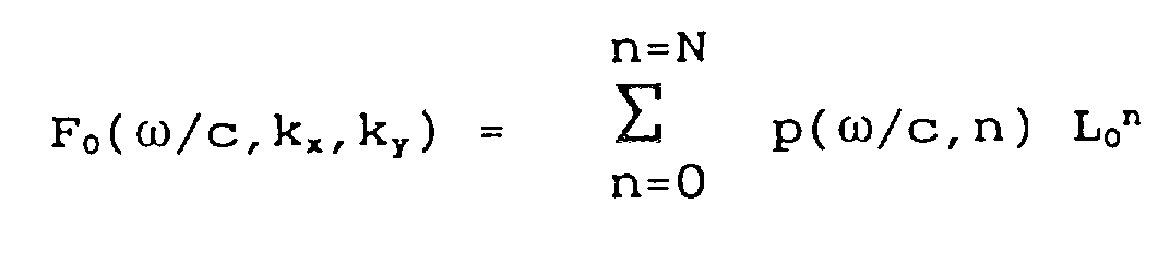
Dans le cas de l'extrapolation à deux dimensions, l'opérateur d'extrapolation s'écrit:![]()
![]()
Les méthodes explicites consistent à faire la synthèse spectrale de F₀, c'est-à-dire calculer une banque de coefficients a(ω/c,n) pour ω/c parcourant un échantillonnage de l'intervalle [ωmin/cmax,ωmax/cmin], où [ωmin,ωmax] représente le contenu fréquentiel des données et [cmin,cmax] les bornes des vitesses de propagation, et n∈[0,N], tels que l'opérateur synthétisé:
Il faut donc assurer la précision sur la bande passante et la stabilité sur la bande d'arrêt.It is therefore necessary to ensure accuracy on the pass band and stability on the stop band.
Holberg [1] utilise pour celà un procédé classique de moindres carrés non linéaire. Cette méthode entraine cependant un coût de calcul élevé.Holberg [1] uses a classical nonlinear least squares method for this. However, this method entails a high calculation cost.
Hale [2] propose un procédé plus rapide en calculant les coefficients a(n) qui égalent les premiers coefficients des développements en série de Taylor de F(k) et F₀(k) en k. La stabilité est assurée en imposant à F(k) d'être nul pour certaines valeurs de k dans la bande d'arrêt. Cependant, une série de Taylor tronquée n'étant une bonne approximation que pour des faibles valeurs de k, donc pour de faibles pendages θ, cette méthode n'est pas optimale.Hale [2] proposes a faster method by calculating the coefficients a (n) which equal the first coefficients of the Taylor series expansions of F (k) and F₀ (k) in k. Stability is ensured by requiring F (k) to be zero for certain values of k in the stop band. However, since a truncated Taylor series is only a good approximation for low values of k, therefore for low dips θ, this method is not optimal.
Dans le cas à 3 dimensions, l'opérateur d'extrapolation d'un champ d'ondes montantes, d'une profondeur Dz pour une vitesse de propagation c et une fréquence ω, est:![]()
![]()
Dans la référence [3] Blaquière propose de réaliser l'extrapolation explicite 3D en généralisant le cas 2D, c'est-à-dire en faisant une synthèse spectrale 2D: une banque de coefficients a(ω/c,nx,ny) est calculée, pour ω/c parcourant un échantillonnage de l'intervalle [ωmin/cmax,ωmax/cmin], où [ωmin,ωmax] représente le contenu fréquentiel des données et [cmin,cmax] les bornes des vitesses de propagation, et nx∈[-Nx,Nx], ny∈[-Ny,Ny], tels que F(ω/c,kx,ky) définit ci-dessous:
Les a(ω/c,nx,ny) sont appliqués de la manière suivante
![]()
![]()
Hale, dans la référence [4], reprend l'idée de la tabulation précédente en tirant partie de surcroit de la symétrie circulaire en (kx,ky) de F₀(ω/c,kx,ky). Il utilise pour celà les coefficients a(ω/c,n) à une dimension correspondant à une extrapolation 2-D et le processus de transformation proposé par McClellan dans la référence [5]. Hale écrit avec Dx=Dy:![]()
et fait la synthèse spectrale:
![]()
and does the spectral synthesis:
Les a(ω/c,n) sont calculés de telle sorte que F(ω/c,k) approxime F₀(ω/c,k) pour les petites valeurs de k et soit partout de module inférieur à 1.The a (ω / c, n) are calculated such that F (ω / c, k) approximates F₀ (ω / c, k) for small values of k and is everywhere of modulus less than 1.
Les cos(nDx k) peuvent se déduire de cos(Dx k) par la formule récursive des polynômes de Chebychev:![]()
![]()
De plus cos(Dx k) peut être approximé par un filtre à deux dimensions pour les pas d'échantillonnage Dx et Dy:
Le développement le plus simple de cos(Dx k) est basé sur la transformée de McClellan à 9 termes, correspondant à NMx=NMy=1:![]()
![]()
Hale propose également d'exploiter une transformée de McClellan améliorée à 17 termes, correspondant à NMx=NMy=2 avec certains termes nuls. Mais, comme on le verra par la suite, même avec cette transformée améliorée, le résultat final comporte des pertubations.Hale also proposes to exploit a McClellan transform improved to 17 terms, corresponding to N Mx = N My = 2 with certain null terms. But, as we will see later, even with this improved transform, the final result involves disturbances.
Plus précisément, la méthode consiste donc à calculer les a(ω/c,n), ω/c parcourant un échantillonnage de l'intervalle [ωmin/cmax, ωmax/cmin] et les M(nx,ny).More precisely, the method therefore consists in calculating the a (ω / c, n), ω / c traversing a sampling of the interval [ω min / c max , ω max / c min ] and the M (n x , n y ).
Définissons l'opération W' = M*W par:
Avec cette notation, le calcul du champ extrapolé Wω,z+dz(mx,my) à partir de Wω,z(mx,my) se fait, pour chaque ω, par le pseudo-code suivant:
- 1) Initialisation :
T₀ = Wz
T₁ = M*Wz
- 2) Itération, pour n=2 jusqu'à N faire:
T = 2 * M * T₁ - T₀
T₁ = T - 3) Fin de la boucle en n.
- 1) Initialization:
T₀ = W z
T₁ = M * W z - 2) Iteration, for n = 2 up to N do:
T = 2 * M * T₁ - T₀
T₁ = T - 3) End of the loop at n.
La présente invention a pour but de perfectionner les techniques existantes de traitement de signaux pour prospection géophysique exploitant un opérateur d'extrapolation d'un champ d'onde.The object of the present invention is to improve existing techniques for processing signals for geophysical prospecting using an operator for extrapolating a wave field.
L'objet de l'invention est en particulier de faciliter le calcul des coefficients des opérateurs de convolution et de simplifier la construction et l'application des opérateurs en 3D.The object of the invention is in particular to facilitate the calculation of the coefficients of the convolution operators and to simplify the construction and application of the operators in 3D.
L'extrapolation du champ d'onde est nécessaire pour réaliser la migration, qui est une étape importante du traitement des données géophysiques. La présente invention peut être appliquée à la migration à 2 ou 3 dimensions, avant ou après sommation, à la migration en profondeur ainsi qu'à la migration en temps. Elle peut s'appliquer aussi à la modélisation, qui est l'opération inverse de la migration.Extrapolation of the wave field is necessary to perform the migration, which is an important step in processing geophysical data. The present invention can be applied to 2 or 3 dimensional migration, before or after summation, to deep migration as well as to time migration. It can also be applied to modeling, which is the reverse operation of migration.
Pour atteindre le but précité il est proposé dans le cadre de la présente invention, un procédé d'extrapolation d'un ensemble de traces enregistrées à l'aide d'un réseau de capteurs, dans un processus de prospection géophysique,
caractérisé par le fait qu'il comprend les étapes consistant à :
- i) approximer un moins Laplacien L₀(kx,ky) = kx 2+ky 2 par la somme de deux filtres à une dimension, et
- ii) approximer un opérateur d'extrapolation Fo par un polynome du moins Laplacien Lo.
characterized by the fact that it comprises the stages consisting in:
- i) approximate a Laplacian minus L₀ (k x , k y ) = k x 2 + k y 2 by the sum of two one-dimensional filters, and
- ii) approximate an extrapolation operator F o by a Laplacian polynomial at least L o .
Selon une caractéristique avantageuse de la présente invention, l'étape i) consiste à approximer le moins Laplacien par la somme de deux filtres à une dimension de la forme:
Selon une autre caractéristique avantageuse de la présente invention, à l'étape ii) l'opérateur d'extrapolation est approximé par un polynome du moins Laplacien de la forme :
Dans le cadre de la présente invention il est également proposé un système pour prospection géophysique du type comprenant :
- une source artificielle d'une onde sonore,
- un réseau de capteurs disposés sur la surface du sol et sensibles aux ondes réfléchies vers le haut par les couches internes du sol,
- un enregistreur relié à ces capteurs pour enregistrer les signaux électriques issus de ceux-ci,
- des moyens de traitement des signaux enregistrés et
- des moyens de visualisation d'un résultat exploitable après traitement de ces signaux,
caractérisé par le fait que :
les moyens de traitement sont adaptés pour décomposer un opérateur d'extrapolation en partie réelle et imagnaire, puis effectuer une synthèse optimale au sens de la norme L-∞ sur chacune des deux parties.
- an artificial source of a sound wave,
- a network of sensors arranged on the ground surface and sensitive to waves reflected upwards by the internal layers of the ground,
- a recorder connected to these sensors to record the electrical signals coming from them,
- means for processing the recorded signals and
- means for displaying an exploitable result after processing these signals,
characterized by the fact that:
the processing means are suitable for decomposing an extrapolation operator into the real and imaginary part, then performing an optimal synthesis within the meaning of the L-∞ standard on each of the two parts.
D'autres buts, caractéristiques et avantages de la présente invention apparaitront à la lecture de description détaillée qui va suivre et en regard des dessins annexés donnés à titre d'exemple non limitatif et sur lesquels:
- la figure 1 représente une vue schématique, sous forme de blocs fonctionnels, d'un système conforme à la présente invention,
- la figure 2a représente la partie réelle d'un filtre d'extrapolation conforme à la présente invention,
- la figure 2b représente le module maximal d'un tel filtre,
- la figure 2c représente la partie imaginaire du filtre d'extrapolation,
- la figure 2d représente le module effectif du filtre d'extrapolation conforme à la présente invention,
- la figure 3 représente la réponse impulsionnelle obtenue en 2 D dans le cadre de la présente invention,
- la figure 4 représente une réponse impulsionnelle 3-D avec utilisation d'un Laplacien à 17 termes conforme à la présente invention, pour une tranche verticale y=0,
- la figure 5 représente une réponse impulsionnelle 3-D avec utilisation d'un Laplacien à 17 termes conforme à la présente invention, pour une tranche horizontale z=450 m,
- la figure 6 représente une réponse impulsionnelle 3-D avec transformée de McClellan à 17 termes conforme à l'état de la technique , pour une tranche horizontale z=450 m.
- FIG. 1 represents a schematic view, in the form of functional blocks, of a system according to the present invention,
- FIG. 2a represents the real part of an extrapolation filter according to the present invention,
- FIG. 2b represents the maximum modulus of such a filter,
- FIG. 2c represents the imaginary part of the extrapolation filter,
- FIG. 2d represents the effective module of the extrapolation filter according to the present invention,
- FIG. 3 represents the impulse response obtained in 2 D in the context of the present invention,
- FIG. 4 represents a 3-D impulse response with the use of a Laplacian with 17 terms in accordance with the present invention, for a vertical section y = 0,
- FIG. 5 represents a 3-D impulse response with the use of a Laplacian with 17 terms in accordance with the present invention, for a horizontal section z = 450 m,
- FIG. 6 represents a 3-D impulse response with McClellan transform in 17 terms conforming to the state of the art, for a horizontal section z = 450 m.
La structure générale du système utilisé dans la présente invention est sensiblement conforme à la structure connue rappelée dans le préambule.The general structure of the system used in the present invention is substantially in accordance with the known structure mentioned in the preamble.
Ce système comprend une source artificielle 10 d'une onde sonore ou ébranlement à base d'explosif ou équivalent, un réseau de capteurs 20, tels que des géophones ou équivalents, disposés sur la surface S du sol et sensibles aux ondes réfléchies vers le haut par les couches internes du sol, un enregistreur 30 relié à ces capteurs 20 pour enregistrer les signaux électriques issus de ceux-ci, sous forme de sismogrammes, des moyens de traitement 40 des signaux enregistrés et des moyens 50 de visualisation d'un résultat exploitable après traitement de ces signaux.This system comprises an
La présente invention se distingue cependant de l'état de la technique par la structure et la fonction des moyens de traitement 40.The present invention differs from the prior art, however, by the structure and the function of the processing means 40.
On va par la suite décrire la fonction de ces moyens de traitement 40 dans le cadre de la présente invention.We will subsequently describe the function of these processing means 40 in the context of the present invention.
Comme indiqué précédemment selon l'invention, on propose d'effectuer la synthèse spectrale en décomposant F₀(k) en partie réelle et imaginaire après une rotation de phase, puis d'effectuer une synthèse optimale au sens de la norme L-∞ sur chacune des deux parties.As indicated previously according to the invention, it is proposed to perform the spectral synthesis by decomposing F₀ (k) into the real and imaginary part after a phase rotation, then to perform an optimal synthesis within the meaning of the standard L-∞ on each of both parties.
Ces 2 synthèses optimales L-∞ peuvent être effectuées par exemple en utilisant le "Remez exchange algorithm" ou "algorithme de Remez", qui est décrit dans la référence [6], et qui résoud le problème suivant:These 2 optimal L-∞ syntheses can be carried out for example using the "Remez exchange algorithm" or "Remez algorithm", which is described in reference [6], and which solves the following problem:
Soit S₀(h) définit pour h∈[0,π], un spectre réel symétrique donné.Let S₀ (h) define for h∈ [0, π], a given symmetric real spectrum.
Soit W(h) définit pour h∈[0,π], une fonction poids réelle positive donné.Let W (h) define for h∈ [0, π], a given positive real weight function.
Soit N la demi-longueur du filtre donnée.
E(h)=W(h)[S(h)-S₀(h)] est la fonction d'erreur pondérée entre le spectre synthétisé et le spectre idéal donné.E (h) = W (h) [S (h) -S₀ (h)] is the weighted error function between the synthesized spectrum and the given ideal spectrum.
Trouver les a(n), n∈[0,N] tels que:Find the a (n), n∈ [0, N] such that:
Norme L-∞ de E(h) = maxh∈[0,π] |E(h)| soit minimum.Norm L-∞ of E (h) = max h∈ [0, π] | E (h) | be minimum.
Plus précisément, la procédure proposée par la présente inventon comprend les étapes qui consistent à:
- i) Décomposer F₀(k) exp(jφc) en parties réelles et imaginaires:

- ii) Par l'algorithme de Remez ou tout autre algorithme, calculer ar(n), n∈[0,N], tels que:

- iii) Puis calculer la fonction de pondération W(k) pour k∈[kc,knyq]:

- iv) Par l'algorithme de Remez ou tout autre algorithme, calculer ai(n), n∈[0,N], tels que:

- i) Decompose F₀ (k) exp (jφ c ) into real and imaginary parts:
- ii) Using Remez's algorithm or any other algorithm, calculate a r (n), n∈ [0, N], such that:
- iii) Then calculate the weighting function W (k) for k∈ [k c , k nyq ]:
- iv) Using Remez's algorithm or any other algorithm, calculate a i (n), n∈ [0, N], such that:
F(k)=[R(k)+jI(k)] ] exp(-jφc) répond alors au problème posé. Les coefficients recherchés sont :![]()
![]()
On a représenté sur la figure 2d annexée le module du filtre d'extrapolation.FIG. 2d shows the module of the extrapolation filter.
La méthode de synthèse spectrale qui vient d'être décrite présente des avantages par rapport aux deux méthodes existantes.The spectral synthesis method which has just been described has advantages over the two existing methods.
L'une (référence [1]) est relativement optimale mais le calcul des coefficients est long, et l'optimalité l'est au sens de la norme L-2. Or, il est préférable que l'approximation en bande passante soit faite pour la norme L-∞, comme dans la méthode proposée En effet ces opérateurs doivent être utilisés de façon récursive. Minimiser l'erreur sur l'opérateur global Fp(k), où p est le nombre de pas d'extrapolation en z, pour n'importe quelle norme, revient en effet à minimiser l'erreur sur l'opérateur unitaire pour la norme L-∞.One (reference [1]) is relatively optimal but the calculation of the coefficients is long, and optimality is within the meaning of the L-2 standard. However, it is preferable that the bandwidth approximation is made for the L-∞ standard, as in the proposed method. Indeed these operators must be used recursively. Minimizing the error on the global operator F p (k) , where p is the number of extrapolation steps in z, for any standard, effectively amounts to minimizing the error on the unit operator for the L-∞ standard.
L'autre (référence [2]) est relativement rapide mais sous-optimale. Elle revient à minimiser l'erreur sur un intervalle local k∈[0,ε] , avec k infiniment petit, alors que la méthode proposée minimise l'erreur sur tout l'intervalle k∈[0,kc=ω sinθ/c], θ étant l'angle maximum de propagation exacte choisi par l'utilisateur, c'est-à-dire que l'erreur est minimisée pour tous les pendages inférieurs à un seuil fixé par l'utilisateur.The other (reference [2]) is relatively fast but suboptimal. It amounts to minimizing the error over a local interval k∈ [0, ε], with k infinitely small, while the proposed method minimizes the error over the entire interval k∈ [0, k c = ω sinθ / c ], θ being the maximum angle of exact propagation chosen by the user, i.e. the error is minimized for all dips below a threshold set by the user.
On a représenté sur la figure 3 la réponse impulsionnelle obtenue pour une plage de fréquence comprise entre fmin = 2Hz et fmax = 48Hz, une vitesse c = 2000 m/s et une cible à une profondeur z = 900m.FIG. 3 shows the impulse response obtained for a frequency range between f min = 2Hz and f max = 48Hz, a speed c = 2000 m / s and a target at a depth z = 900m.
Comme indiqué précédemment, l'un des buts importants de la présente invention est de simplifier le processus de calcul mis en oeuvre pour extrapoler le champ d'onde 3-D représenté par les traces enregistrées, et en améliorer la précision.As indicated above, one of the important aims of the present invention is to simplify the calculation process used to extrapolate the 3-D wave field represented by the recorded traces, and to improve its precision.
Ce but est atteint selon la présente invention grâce à un procédé d'extrapolation en profondeur d'un champ d'onde enregistré à l'aide d'un réseau de capteurs dans un processus de prospection géophysique comprenant les étapes qui consistent à mettre l'opérateur d'extrapolation sous la forme:![]()
![]()
![]()
![]()
Plus précisément selon l'invention le procédé d'extrapolation comprend les étapes qui consistent à :
- i) approximer un moins Laplacien L₀(kx,ky) = kx 2+ky 2 par la somme de deux filtres à une dimension, et
- ii) approximer un opérateur d'extrapolation Fo par un polynome du moins Laplacien Lo.
- i) approximate a Laplacian minus L₀ (k x , k y ) = k x 2 + k y 2 by the sum of two one-dimensional filters, and
- ii) approximate an extrapolation operator F o by a Laplacian polynomial at least L o .
Le moins Laplacien est de préférence approximé par la somme de deux filtres à une dimension de la forme:
Par ailleurs à l'étape ii) l'opérateur d'extrapolation est de préférence approximé par un polynome du moins Laplacien de la forme :
L'opérateur moins Laplacien L₀ peut être scindé, sans approximation, sous forme de la somme de deux opérateurs de moins dérivée seconde, chacun d'eux pouvant être approximé par un filtre à une dimension avec NLx et NLy termes en cosinus.The minus Laplacian operator L₀ can be split, without approximation, into the sum of two minus second derivative operators, each of which can be approximated by a one-dimensional filter with N Lx and N Ly cosine terms.
La présente invention exploite la symétrie circulaire de l'opérateur d'extrapolation, comme le propose Hale dans le cadre d'une mise en oeuvre de transformée de McClellan.The present invention exploits the circular symmetry of the extrapolation operator, as Hale proposes in the context of a McClellan transform implementation.
Cependant la présente invention permet d'éviter le calcul du filtre 2-D approximant cos[Dx(kx 2+ky 2)1/2] grâce à l'utilisation d'un opérateur moins Laplacien, L₀ = kx 2 + ky 2, à l'aide duquel l'opérateur d'extrapolation F₀ est developpé sous la forme de polynome et dont la synthèse ne nécessite que des filtres 1-D.However, the present invention makes it possible to avoid the calculation of the 2-D filter approximating cos [Dx (k x 2 + k y 2 ) 1/2 ] thanks to the use of a less Laplacian operator, L₀ = k x 2 + k y 2 , using which the extrapolation operator F₀ is developed in the form of a polynomial and the synthesis of which requires only 1-D filters.
Plus précisément, la procédure proposée dans le cadre de la présente invention comprend les étapes qui consistent à:
- 1) Faire une synthèse spectrale de l'opérateur moins dérivée seconde en x, c'est-à-dire calculer un filtre symétrique de longueur 2NLx+1, pour le pas d'échantillonnage Dx, dont le spectre Dx(k), définit par :

avec 0 < αx< 1 (αx est typiquement égal à 0,7). Aucune contrainte n'est imposée à Dx(k) sur k∈[αxknyqx,knyqx] (lorsque αx est petit, on peut éventuellement imposer à Dx(k) de ne pas dépasser une certaine valeur). - 2) Faire la même chose pour y:

- 3) Définir L(kx,ky) = Dx(kx) + Dy(ky) qui est la synthèse spectrale du moins Laplacien L₀(kx,ky)=kx 2+ky 2 sur le rectangle kx∈[-αxknyqx,αxknyqx], ky∈[-αyknyqy,αyknyqy].
- 1) Make a spectral synthesis of the operator less derivative second in x, that is to say calculate a symmetrical filter of length 2N Lx +1, for the sampling step Dx, whose spectrum D x (k) , defined by:
- 2) Do the same for y:
- 3) Define L (k x , k y ) = D x (k x ) + D y (k y ) which is the spectral synthesis of the Laplacian least L₀ (k x , k y ) = k x 2 + k y 2 on the rectangle k x ∈ [-α x k nyqx , α x k nyqx ], k y ∈ [-α y k nyqy , α y k nyqy ].
En pratique, on calcule d'abord les dx(n), dy(n) (qui sont a priori indépendants de ω/c mais qui peuvent aussi en dépendre). Ensuite les bornes [Lmin,Lmax] de L(kx,ky) sont calculées en tant que somme des bornes de Dx(k) et de Dy(k). On choisit θ qui est l'angle de propagation maximum considéré par rapport à la verticale. Pour une pulsation et une vitesse donnée, celà correspond à un nombre d'onde kc=ωsinθ/c. Puis pour chaque ω/c parcourant un échantillonnage de l'intervalle [ωmin/cmax,ωmax/cmin], on calcule les p( ω/c,n), en tant que développement polynomial de F₀(ω/c,L). F(ω/c,L) doit approximer F₀(ω/c,L) pour L∈[Lmin,Lc=kc 2=ωsinθ/c] et doit être de module inférieur à 1 pour L∈[Lc,Lmax].In practice, we first calculate the d x (n), d y (n) (which are a priori independent of ω / c but which can also depend on it). Then the bounds [L min , L max ] of L (k x , k y ) are calculated as the sum of the bounds of D x (k) and D y (k). We choose θ which is the maximum propagation angle considered with respect to the vertical. For a given pulse and speed, this corresponds to a wave number k c = ωsinθ / c. Then for each ω / c traversing a sampling of the interval [ω min / c max , ω max / c min ], we calculate the p (ω / c, n), as a polynomial expansion of F₀ (ω / c , L). F (ω / c, L) must approximate F₀ (ω / c, L) for L∈ [L min , L c = k c 2 = ωsinθ / c] and must be of module less than 1 for L∈ [L c , L max ].
Définissons l'opération W'=L*W par:
W' approxime le moins Laplacien de W.W 'approximates the least Laplacian of W.
Avec cette notation, le calcul du champ extrapolé Wω,z+dz(mx,my) à partir de Wω,z(mx,my) se fait, pour chaque ω, par le pseudo-code comprenant les étapes qui consistent à:
- 1) Initialiser:

- 2) Pour n=N-1
jusqu'à 0 faire:
- 1) Initialize:
- 2) For n = N-1 up to 0 do:
On va maintenant préciser la méthode proposée dans le cadre de la présente invention pour calculer les coefficients en extrapolation 3D.We will now specify the method proposed in the context of the present invention for calculating the coefficients in 3D extrapolation.
Nous avons vu comment ramener la synthèse de F₀(ω/c,kx,ky) à celle de coefficients 1-D: une synthèse polynomiale 1-D, p(ω/c,n), et deux synthèses spectrales 1-D de spectres réels symétriques, dx(n) et dy(n). Nous allons décrire une procédure de calcul pour ces coefficients.We have seen how to reduce the synthesis of F₀ (ω / c, k x , k y ) to that of coefficients 1-D: a polynomial synthesis 1-D, p (ω / c, n), and two spectral syntheses 1- D of symmetric real spectra, d x (n) and d y (n). We will describe a calculation procedure for these coefficients.
Les synthèses de dx(n) et dy(n) peuvent se faire simplement en utilisant l'algorithme de Remez, avec S₀(h)=h, W(h)=1 pour h∈[0,αxπ],W(h)=ε pour h∈[αxπ,π], où ε est un petit nombre de l'ordre de 0,05.The syntheses of d x (n) and d y (n) can be done simply by using the Remez algorithm, with S₀ (h) = h, W (h) = 1 for h∈ [0, α x π] , W (h) = ε for h∈ [α x π, π], where ε is a small number on the order of 0.05.
On montre que la synthèse polynomiale peut se ramener à une synthèse spectrale. De plus celle-ci peut être opérée avec le procédé décrit précédemment pour l'extrapolation 2D.We show that polynomial synthesis can be reduced to spectral synthesis. In addition it can be operated with the method described above for 2D extrapolation.
La synthèse polynomiale à effectuer est la suivante:The polynomial synthesis to be performed is as follows:
Soit une fonction complexe F₀(L) donnée, ainsi qu'un intervalle [Lmin,Lmax] et une valeur Lc. Il faut trouver des coefficients p(n), n∈[0,N], tels que:
une approximation de F₀(L) sur [Lmin,Lc] et que le module de F(L) soit inférieur à 1 sur [Lc,Lmax].Let be a given complex function F₀ (L), as well as an interval [L min , L max ] and a value L c . We must find coefficients p (n), n∈ [0, N], such that:
an approximation of F₀ (L) on [L min , L c ] and that the modulus of F (L) is less than 1 on [L c , L max ].
Faisons le changement de variable:![]()
![]()
F₀[g(h)] = S₀(h) est un spectre symétrique connu.F₀ [g (h)] = S₀ (h) is a known symmetric spectrum.
Posons hc = g⁻¹(Lc).Let h c = g⁻¹ (L c ).
On résoud le problème de synthèse spectrale suivant, en utilisant par exemple la méthode proposée précédemment :We solve the following spectral synthesis problem, using for example the method proposed above:
Trouver les t(n), n∈[0,N], tels que
Les t(n) définissants S(h) étant calculés, la méthode décrite dans la suite, F(L)=S(g⁻¹(L)) répond au problème posé.The t (n) defining S (h) being calculated, the method described below, F (L) = S (g⁻¹ (L)) answers the problem posed.
En effet, le changement de variable L=g(h) transforme un polynôme de degré N en L en un polynôme de degré N en cos(h) et donc, d'après les polynômes de Chebychev, en une somme de cos(nh) pour n variant de 0 à N. Donc réciproquement, h=g⁻¹(L), transforme un spectre de cosinus en un polynôme. De plus, la norme L-∞ est invariante par changement de variable. Donc si la synthèse spectrale est optimale pour la norme L-∞, la synthèse polynomiale le sera aussi.Indeed, the change of variable L = g (h) transforms a polynomial of degree N in L into a polynomial of degree N in cos (h) and therefore, according to Chebychev's polynomials, into a sum of cos (nh ) for n varying from 0 to N. So reciprocally, h = g⁻¹ (L), transforms a cosine spectrum into a polynomial. In addition, the norm L-∞ is invariant by change of variable. So if the synthesis spectral is optimal for the L-∞ norm, so will the polynomial synthesis.
Plus précisément, on peut écrire F(L) sous la forme:
Tn(x) étant le polynôme de Chebychev de degré n définit par Tn(cos h) = cos nh.T n (x) being the Chebychev polynomial of degree n defined by T n (cos h) = cos nh.
On se ramène ensuite à la forme:
Le passage de la forme (4) à la forme (5) pour F(L) se fait en écrivant:

Les a(m,n) se calculent récursivement en écrivant:![]()
![]()
Lorsque N est grand, il peut être impossible de trouver un A qui permette de ne pas avoir de problèmes de précision machine. Dans ce cas, il faut en rester à la forme en polynômes de Chebychev (4). Le pseudo-code de la méthode devient alors similaire à celui de la méthode de Hale, mais l'opérateur M, qui a une forme rectangulaire dans le domaine (x,y) est remplacé par l'opérateur (2L-Lmin-Lmax)/(Lmin-Lmax) qui a une forme de croix dans le domaine (x,y).When N is large, it may be impossible to find an A which allows not to have problems of machine precision. In this case, it is necessary to stick to the form in Chebychev polynomials (4). The pseudo-code of the method then becomes similar to that of the method of Hale, but the operator M, which has a rectangular shape in the domain (x, y) is replaced by the operator (2L-L min -L max ) / (L min -L max ) which has a cross shape in the domain (x, y).
Avec la forme (4) de F(L), le pseudo-code utilisé est le suivant :
- 1) initialiser :
T₀=Wz
T₁=L*Wz,
- 2) Pour n=2 jusqu'à N faire:
T=2*L*T₁-T₀
T₁=T
Fin de la boucle en n
avec W'=L*W définit par
- 1) initialize:
T₀ = W z
T₁ = L * W z , - 2) For n = 2 to N do:
T = 2 * L * T₁-T₀
T₁ = T
End of loop in n
with W '= L * W defined by
Avec la forme (5) de F(L), le pseudo-code utilisé est le suivant :
- 1) initialiser

- 2) Pour n=N-1
jusqu'à 0 faire:

- 1) initialize
- 2) For n = N-1 up to 0 do:
L'extrapolation en temps d'un champ d'onde permet de faire la migration en temps, avant ou après sommation, une étape souvent utilisée en traitement géophysique. La migration en temps est moins précise que la migration en profondeur, mais elle peut se contenter d'un modèle de vitesse cz(mx,my) beaucoup moins précis, ce qui en fait l'utilité.Extrapolation in time of a wave field makes it possible to migrate in time, before or after summation, a step often used in geophysical processing. Time migration is less precise than deep migration, but it can be content with a much less precise speed model c z (m x , m y ), which makes it useful.
Contrairement aux méthodes de l'état de la technique précédemment décrites, la méthode proposée par la présente invention peut s'étendre au cas de l'extrapolation en temps. La fonction d'extrapolation en kx,ky est dans ce cas, pour un pas d'extrapolation temporel Dt:![]()
![]()
G₀(ω,c) dépend cette fois-ci séparément de ω et de c et ne peut se mettre sous la forme G₀(ω/c). Une méthode basée sur la tabulation nécessiterait un filtre pour chaque ω et chaque c, ce qui serait prohibitif en temps de calcul et en stockage.G₀ (ω, c) this time depends separately on ω and c and cannot be put in the form G₀ (ω / c). A tabulation-based method would require a filter for each ω and each c, which would be prohibitive in computation time and storage.
La méthode proposée, utilisant un développement en monômes de la forme Ln, permet de ne tabuler les coefficients que pour la vitesse minimale cmin, et de déduire les coefficients correspondant à une vitesse c quelconque par une opération très simple qui peut être faite au moment de l'application.The proposed method, using a development in monomials of the form L n , makes it possible to tabulate the coefficients only for the minimum speed c min , and to deduce the coefficients corresponding to any speed c by a very simple operation which can be done at the time of application.
On écrit:
On précalcule et tabule les p(ω,cmin,n) pour un échantillonnage de ω∈[ωmin,ωmax]. Pour une vitesse c quelconque, écrivons:
Donc p(ω,c,n) = (c/cmin)2np(ω,cmin,n) fournit une approximation de G₀(ω,c,kx,ky).So p (ω, c, n) = (c / c min ) 2n p (ω, c min , n) provides an approximation of G₀ (ω, c, k x , k y ).
Les p(ω,cmin,n) doivent être calculés sur [Lmincmax 2/cmin 2,Lmaxcmax 2/cmin 2] au lieu de [Lmin,Lmax]. De cette façon, la stabilité (le fait que le module ne soit jamais supérieur à 1), est assurée pour toutes les vitesses c et non pas seulement pour la vitesse tabulée. La tabulation se fait avec Lc=ωsinθ/cmin 2, de sorte que cette valeur de Lc est plus grande que les valeurs de Lc nécessaires pour les autres vitesses. C'est la raison pour laquelle il faut tabuler pour cmin plutôt que pour un c₀ arbitraire.The p (ω, c min , n) must be calculated on [L min c max 2 / c min 2 , L max c max 2 / c min 2 ] instead of [L min , L max ]. In this way, stability (the fact that the module is never greater than 1) is ensured for all speeds c and not only for the tabulated speed. The tabulation is done with L c = ωsinθ / c min 2 , so that this value of L c is greater than the values of L c necessary for the other speeds. This is the reason why it is necessary to tabulate for c min rather than for an arbitrary c₀.
Si le rapport cmax/cmin est trop grand, on peut tabuler pour 2 ou 3 valeurs de c: cmin,cint1,cint2,..., et se baser pour calculer p(ω,c,n) sur la valeur tabulée juste inférieure à c.If the ratio c max / c min is too large, we can tabulate for 2 or 3 values of c: c min , c int1 , c int2 , ..., and use it to calculate p (ω, c, n) on the tabulated value just below c.
Le procédé conforme à la présente invention offre des avantages notables par rapport à la technique antérieure, en particulier par rapport au procédé proposé par Hale dans la référence [4].The process according to the present invention offers significant advantages over the prior art, in particular over the process proposed by Hale in reference [4].
Tout d'abord le procédé conforme à la présente invention, basé sur un développement polynomial et une synthèse spectrale de Laplacien, requiert seulement le calcul et l'application d'une banque de coefficients polynomiaux à une dimension p(ω/c,n) et de deux filtres symétriques à une dimension dx(n) et dy(n); alors que le procédé proposé par HaIe, requiert le calcul et l'application d'une banque de filtres à une dimension b(ω/c,n) et d'un filtre à deux dimensions M(nx,ny) (transformée de McClellan à 9 ou 17 termes par exemple). La méthode de la référence [3] requiert pour sa part le calcul et l'application d'une banque de filtres à deux dimensions a(ω/c,nx,ny) et est donc beaucoup plus lourde.First of all the method according to the present invention, based on a polynomial development and a Laplacian spectral synthesis, only requires the calculation and the application of a bank of polynomial coefficients to a dimension p (ω / c, n) and two symmetrical one-dimensional filters d x (n) and d y (n); whereas the method proposed by HaIe, requires the calculation and application of a bank of filters with a dimension b (ω / c, n) and a two-dimensional filter M (n x , n y ) (transformed of McClellan with 9 or 17 terms for example). The method of reference [3] for its part requires the calculation and application of a bank of two-dimensional filters a (ω / c, n x , n y ) and is therefore much more cumbersome.
Par ailleurs, nous avons montré que le calcul d'un développement polynomial se ramène à celui d'un spectre symétrique. On peut donc utiliser pour le développement polynomial le même algorithme que pour le développement spectral. Les approximations polynomiales et spectrales ont alors une précision similaire, pour un nombre de termes identiques.Furthermore, we have shown that the computation of a polynomial expansion is reduced to that of a symmetric spectrum. We can therefore use the same algorithm for polynomial development as for spectral development. The polynomial and spectral approximations then have a similar precision, for a number of identical terms.
Enfin avec un nombre de termes identique, la synthèse spectrale du Laplacien donne une meilleure précision que la synthèse spectrale de la fonction cos[Dx(kx 2+ky 2)1/2] dont la transformée de McClellan est un cas particulier. Avec la méthode proposée, n'ayant que des spectres symétriques à une dimension à calculer, nous pouvons utiliser des algorithmes optimaux et rapides. De plus, l'application d'un Laplacien, qui a une forme de croix dans le domaine (x,y) est plus rapide que l'application d'un cos[Dx(kx 2+ky 2)1/2] , qui a une forme rectangulaire.Finally with an identical number of terms, the Laplacian spectral synthesis gives better precision than the spectral synthesis of the cos function [Dx (k x 2 + k y 2 ) 1/2 ] of which the McClellan transform is a particular case. With the proposed method, having only one-dimensional symmetric spectra to calculate, we can use optimal and fast algorithms. In addition, the application of a Laplacian, which has a cross shape in the domain (x, y) is faster than the application of a cos [Dx (k x 2 + k y 2 ) 1/2 ], which has a rectangular shape.
D'autre part, le cas Dx≠Dy, qui est le plus courant en pratique, complique la méthode de Hale alors qu'elle ne pose aucun problème avec la méthode proposée.On the other hand, the case Dx ≠ Dy, which is the most common in practice, complicates the Hale method while it poses no problem with the proposed method.
Un autre avantage notable de la méthode proposée est que l'extrapolation en temps est possible avec une table à une dimension, alors qu'elle nécessiterait une table à deux dimensions avec les méthodes existantes (ce qui la rend non pratiquable).Another notable advantage of the proposed method is that time extrapolation is possible with a one-dimensional table, whereas it would require a two-dimensional table with existing methods (which makes it impractical).
La figure 4 représente une tranche verticale pour y=0 d'une réponse impulsionnelle correspondant à:FIG. 4 represents a vertical section for y = 0 of an impulse response corresponding to:
Dx=Dy=Dz=10m, c=1000m/s, θ=60 degrés, fmin=2Hz, fmax=48Hz, z=900m, NLx=NLy=4 de sorte que le Laplacien comprend 17 coefficients. Le développement polynomial est de degré 15.Dx = Dy = Dz = 10m, c = 1000m / s, θ = 60 degrees, f min = 2Hz, f max = 48Hz, z = 900m, N Lx = N Ly = 4 so that the Laplacian has 17 coefficients. The polynomial development is of degree 15.
La figure 5 représente une tranche horizontale obtenue dans le cadre de la présente invention à l'aide d'un procédé mettant en oeuvre un développement polynomial à 15 termes et une synthèse de Laplacien à 17 termes, pour z=450m, soit un angle de 60 degrés.FIG. 5 represents a horizontal slice obtained within the framework of the present invention using a method implementing a polynomial development in 15 terms and a Laplacian synthesis in 17 terms, for z = 450m, that is to say an angle of 60 degrees.
La figure 6 représente une tranche horizontale obtenue à l'aide d'un procédé classique comprenant un développement spectral à 12 termes et une transformée de McClellan à 17 termes, pour la même profondeur z=450m. Le développement spectral à 12 termes est calculé par la méthode de synthèse spectrale par 2 optimisations L-∞ décrite précédemment.FIG. 6 represents a horizontal slice obtained using a conventional method comprising a spectral development at 12 terms and a McClellan transform at 17 terms, for the same depth z = 450m. The spectral development with 12 terms is calculated by the method of spectral synthesis by 2 optimizations L-∞ described previously.
On peut noter que les perturbations visibles sur la figure 6, ne possèdent pas de symétrie circulaire. Il est donc clair qu'elles ne résultent pas d'une erreur dans le développement à 12 termes, mais nécessairement dans la transformée de McClellan à 17 termes.It can be noted that the disturbances visible in FIG. 6 do not have circular symmetry. he it is therefore clear that they do not result from an error in the 12-term development, but necessarily in the 17-term McClellan transform.
Références bibliographiques:Bibliographic references:
- [1] O. Holberg: Towards Optimum one-way Wave Propagation, Geophysical Prospecting, vol.36 n°2, pp. 99-114, Février 1988.[1] O. Holberg: Towards Optimum one-way Wave Propagation, Geophysical Prospecting, vol.36 n ° 2, pp. 99-114, February 1988.
- [2] D. Hale: Stable, Explicit Depth Extrapolation of Seismic Wavefields, Geophysics, vol.56 n°11, pp. 1770-1777, Novembre 1991.[2] D. Hale: Stable, Explicit Depth Extrapolation of Seismic Wavefields, Geophysics, vol.56 n ° 11, pp. 1770-1777, November 1991.
- [3] G. Blaquiere, H.W.J. Debeye, C.P.A. Wapenaar, A.J. Berkhout: 3-D table-driven Migration, Geophysical Prospecting, vol.37 n°8, pp. 925-958, Novembre 1989.[3] G. Blaquiere, H.W.J. Debeye, C.P.A. Wapenaar, A.J. Berkhout: 3-D table-driven Migration, Geophysical Prospecting, vol.37 n ° 8, pp. 925-958, November 1989.
- [4] D. Hale: 3-D Depth Migration via McClellan Transformations, Geophysics, vol.56 n°11, pp. 1778-1785, Novembre 1991.[4] D. Hale: 3-D Depth Migration via McClellan Transformations, Geophysics, vol.56 n ° 11, pp. 1778-1785, November 1991.
- [5] J.H. McClellan: The Design of Two-Dimensional Filters by Transformations, Proc. 7th Annual Princeton Conf. on Inform. Sci. and Syst., pp. 247-251,1973.[5] J.H. McClellan: The Design of Two-Dimensional Filters by Transformations, Proc. 7th Annual Princeton Conf. on Inform. Sci. and Syst., pp. 247-251.1973.
- [6] J.H. McClellan, T.W. Parks: Equiripple Approximation of Fan Filters, Geophysics, vol.37 n°4, pp. 573-583, Août 1972.[6] J.H. McClellan, T.W. Parks: Equiripple Approximation of Fan Filters, Geophysics, vol.37 n ° 4, pp. 573-583, August 1972.
Claims (40)
- A method of extrapolating a set of traces recorded by means of an array of sensors in a geophysical prospecting process,
the method being characterized by the fact that it comprises the steps consisting in:i) approximating a minus Laplacian L₀(kx,ky) = kx 2+ky 2 by the sum of two one-dimensional filters; andii) approximating an extrapolation operator F₀ by a polynomial of the minus Laplacian L₀. - A method according to claim 1, characterized by the fact that step i) consists in approximating the minus Laplacian by the sum of two one-dimensional filters of the form:

- A method according to claim 1 or 2, characterized by the fact that step ii) of the extrapolation operator is approximated by a polynomial of the minus Laplacian of the form:
- A method according to claim 1 or 3, characterized by the fact that synthesis of the minus Laplacian consists in:1) performing spectrum synthesis of the minus second derivative operator in x, by calculating a symmetrical filter of length 2NLx+1 with a sampling interval Dx, where the spectrum Dx(k) defined by:
 2) performing spectrum synthesis of the minus second derivative operator in y by calculating a symmetrical filter of length 2NLy+1 for a sampling step size Dy, whose spectrum Dy(k) defined by:
 3) defining L(kx,ky) = Dx(kx) + Dy(ky) which is the spectrum synthesis of the minus Laplacian L₀(kx,ky)=kx 2+ky 2 over the rectangle kx∈[-αxknyqx,αxknyqx], ky∈[-αyknyqy,αyknyqy].
 - A method according to any one of claims 1 to 4, characterized by the fact that the coefficients dx(n) and dy(n) of the minus Laplacian are synthesized by using the Remez algorithm, with S₀(h)=h, W(h)=1 for h∈[0,αx,π], W(h)=ε for h∈[αx,π,π] where ε is a small number equal to about 0.05.
- A method according to any one of claims 1 to 5, characterized by the fact that the polynomial synthesis of the extrapolation operator is performed in the form of a spectrum synthesis.
- A method according to any one of claims 1 to 6, characterized by the fact that the depth extrapolation consists in:computing the coefficients dx(n) and dy(n) of the minus Laplacian;computing the limits [Lmin,Lmax] of the minus Laplacian; andfor each ω/c running over sampling in the range [ωmin/cmax,ωmax/cmin] calculating the coefficients p(ω/c,n) of the polynomial development of the extrapolation operator F₀(ω/c,L).
- A method according to any one of claims 1 to 7, characterized by the fact that the depth extrapolation consists in:1) initializing
 2) for n=N-1 to 0 doing:

- A method according to any one of claims 1 to 8, characterized by the fact that the polynomial synthesis of the extrapolation operator is performed on the basis of steps consisting in:
changing variable:
finding t(n), n∈[0,N] such that
- A method according to any one of claims 1 to 9, characterized by the fact that it includes the step consisting in writing the extrapolation operation in the form:

- A method according to any one of claims 1 to 10, characterized by the fact that it includes the step consisting in writing the extrapolation operator in the form:

- A method according to any one of claims 1 to 11, characterized by the fact that depth extrapolation consists in:1) initializing
 2) for n=N-1 to 0 doing:

- A method according to any one of claims 1 to 12, characterized by the fact that depth extrapolation consists in:1) initializing:
T₀ = Wz
T₁ = L*Wz 2) for n = 2 to N doing:
T = 2 * L * T₁ - T₀
T₁ = T
end n loop
with W'=L*W defined by
- A method according to any one of claims 1 to 13, characterized by the fact that it further includes a time 3D extrapolation stage on the basis of the extrapolation function which is written for one time extrapolation step Dt:

tabulating the coefficients p(ω,cmin,n) of the polynomial development for at least one determined velocity value (cmin); and
calculating the other required coefficients p(ω,c,n) by multiplying the tabulated coefficients by (c/cmin)2n, i.e.
- A method according to any one of claims 1 to 14, characterized by the fact that it includes the step consisting in splitting an extrapolation operator (20) into a real part and an imaginary part, and then in performing synthesis that is optimum in the L-∞ sense on each of the two parts.
- A method according to claim 15, characterized by the fact that the L-∞ optimum synthesis on the real part and on the imaginary part of the extrapolation operator is performed by using the Remez algorithm.
- A method according to claim 15 or 16, characterized by the fact that the optimum synthesis of the real part and of the imaginary part of the extrapolation operator consists in looking for a(n), n∈[0,N] of the synthesized spectrum:
 L-∞ norm of E(h) = maxh∈[0,π] |(E(h)| is a minimum with:S₀ defining for h∈[0,π] a given symmetrical real spectrum;W(h) defining for h∈[0,π] a given positive real weighting function;N being the half-length of the given filter; andE(h)=W(h)[S(h)-S₀(h)] being the weighted error function between the synthesized spectrum and the given ideal spectrum.
 - A method according to any one of claims 15 to 17, characterized by the fact that the extrapolation operator is synthesized by means of the steps consisting in:i) splitting the extrapolation operator F₀(k) exp(jφc) into real and imaginary parts;
 ii) calculating ar(n), n∈[0,N], such that
 iii) calculating the weighting function W(k) for k∈[kc,knyq]:
 iv) calculating ai(n), n∈[0,N] such that:
 v) defining the extrapolation operator by summing the syntheses obtained in steps ii) and iv), i.e.:

- A method according to any one of claims 15 to 18, characterized by the fact that in step i), the following is set:
- A method according to any one of claims 15 to 19, characterized by the fact that in step iii) the minimum of M(k) is constrained to be greater than α and its maximum is constrained to be less than one.
- A geophysical prospecting system of the type comprising:an artificial soundwave source (10);an array of sensors (20) disposed on the surface of the ground and sensitive to waves reflected upwards by the internal strata of the ground;a recorder (30) connected to said sensors for recording the electrical signals from them;processor means (40) for processing the recorded signals; anddisplay means (50) for displaying a usable result after processing the signals;the system being characterized by the fact that the processor means (40) are adapted to split an extrapolation operator (20) into a real part and an imaginary part, and then to perform synthesis that is optimum in the L-∞ norm sense on each of the two parts.
- A system according to claim 21, characterized by the fact that the processor means (40) perform L-∞ optimum synthesis on the real part and on the imaginary part of the extrapolation operator with the help of the Remez algorithm.
- A system according to any one of claims 21 to 22, characterized by the fact that the processor means (40) perform optimum synthesis of the real part and of the imaginary part of the extrapolation operator by searching for a(n), n∈[0,N] of the synthesized spectrum:

with:S₀ defining a given symmetrical real spectrum for h∈[0,π];W(h) defining a given positive real weighting function for h∈[0,π];N being the given filter half-length; andE(h)=W(h)[S(h)-S₀(h)] being the weighted error function between the synthesized spectrum and the given ideal spectrum. - A system according to any one of claims 21 to 23, characterized by the fact that the processor means (40) synthesize the extrapolation operator with the help of steps consisting in:i) splitting the extrapolation operator F₀(k) exp(jφc) into real and imaginary parts;
 ii) calculating ar(n), n∈[0,N], such that
 iii) calculating the weighting function W(k) for k∈[kc,knyq]:
 iv) calculating ai(n), n∈[0,N] such that:
 v) defining the extrapolation operator by summing the syntheses obtained in steps ii) and iv), i.e.:

- A system according to any one of claims 21 to 24, characterized by the fact that at step i) the processor means (40) set:

- A system according to any one of claims 21 to 25, characterized by the fact that at step iii) the processor means (40) constrain the minimum of M(k) to be greater than α and its maximum to be less than one.
- A system according to any one of claims 21 to 26, characterized by the fact that the processor means are adapted to:i) approximate a minus Laplacian L₀(kx,ky) = kx 2+ky 2 by the sum of two one-dimensional filters; andii) approximate an extrapolation operator F₀ by a polynomial of the minus Laplacian L₀.
- A system according to claim 27, characterized by the fact that at step i) the processor means (40) approximate the minus Laplacian by the sum of two one-dimensional filters of the form:

- A system according to any one of claims 27 to 28, characterized by the fact that at step ii) the processor means (40) approximate the extrapolation operator by a polynomial of the minus Laplacian of the form:

- A system according to any one of claims 21 to 29, characterized by the fact that to synthesize the minus Laplacian, the processor means are adapted to:1) perform spectrum synthesis of the minus second derivative operator in x, by calculating a symmetrical filter of length 2NLx+1 with a sampling interval Dx, where the spectrum Dx(k) defined by:
 2) performing spectrum synthesis of the minus second derivative operator in y by calculating a symmetrical filter of length 2NLy+1 with a sampling interval Dy, whose spectrum Dy(k) defined by:
 3) defining L(kx,ky) = Dx(kx) + Dy(ky) which is the spectrum synthesis of the minus Laplacian L₀(kx,ky)=kx 2+ky 2 over the rectangle kx∈[-αxknyqx,αxknyqx], ky∈[-αyknyqy, αyknyqy].
 - A system according to any one of claims 21 to 30, characterized by the fact that the coefficients dx(n) and dy(n) of the minus Laplacian are synthesized by the processor means (40) by using the Remez algorithm, with S₀(h)=h, W(h)=1 for h∈[0,αx,π], W(h)=ε for h∈[αx,π,π] where ε is a small number equal to about 0.05.
- A system according to any one of claims 21 to 31, characterized by the fact that the polynomial of the extrapolation operator is synthesized by the processor means (40) in the form of a spectrum synthesis.
- A system according to any one of claims 21 to 32, characterized by the fact that the processor means (40) form depth extrapolation with the help of steps that consist in:calculating the coefficients dx(n) and dy(n) of the minus Laplacian;defining the limits [Lmin,Lmax] of the minus Laplacian; andfor each ω/c running over sampling in the range [ωmin/cmax,ωmax/cmin] calculating the coefficients p(ω/c,n) of the polynomial development of the extrapolation operator F₀(ω/c,L).
- A system according to any one of claims 21 to 33, characterized by the fact that for depth extrapolation, the processor means (40) are adapted to:1) initializing
 2) for n=N-1 to 0 doing:

- A system according to any one of claims 21 to 34, characterized by the fact that the polynomial of the extrapolation operator is synthesized by the processor means (40) on the basis of steps consisting in:
changing variable:
L = ½(Lmin-Lmax) cos(h) + ½(Lmin+Lmax) = g(h) with L∈[Lmin,Lmax], h∈[0,π], and
F₀[g(h)] = S₀(h) being a known symmetrical spectrum finding t(n), n∈[0,N] such that
- A system according to any one of claims 21 to 35, characterized by the fact that the processor means (40) write the extrapolation operator in the form:

- A system according to any one of claims 21 to 36, characterized by the fact that the processor means (40) write the extrapolation operator in the form:

- A system according to any one of claims 21 to 37, characterized by the fact that for depth extrapolation the processor means (40) are adapted to:1) initializing
 2) for n=N-1 to 0 doing:

- A system according to any one of claims 21 to 38, characterized by the fact that for depth extrapolation, the processor means (40) are adapted to:1) initializing:
T₀ = Wz
T₁ = L*Wz 2) for n = 2 to N doing:
T = 2 * L * T₁ - T₀
T₁ = T
end n loop
with W'=L*W defined by
- A system according to any one of claims 21 to 39, characterized by the fact that the processor means (40) are adapted to operate a time 3D extrapolation stage on the basis of the extrapolation function which is written as follows for one time extrapolation step Dt:

tabulating the coefficients p(ω,cmin,n) of the polynomial development for at least one determined velocity value (cmin); and
calculating the other required coefficients p(ω,c,n) by multiplying the tabulated coefficients by (c/cmin)2n, i.e.
Applications Claiming Priority (2)
| Application Number | Priority Date | Filing Date | Title |
|---|---|---|---|
| FR9206564 | 1992-05-29 | ||
| FR929206564A FR2691812B1 (en) | 1992-05-29 | 1992-05-29 | Signal processing method for geophysical prospecting using an operator to extrapolate an improved wave field. |
Publications (2)
| Publication Number | Publication Date |
|---|---|
| EP0572321A1 EP0572321A1 (en) | 1993-12-01 |
| EP0572321B1 true EP0572321B1 (en) | 1996-04-03 |
Family
ID=9430282
Family Applications (1)
| Application Number | Title | Priority Date | Filing Date |
|---|---|---|---|
| EP93401354A Expired - Lifetime EP0572321B1 (en) | 1992-05-29 | 1993-05-27 | Signal processing process for geophysical exploration, using an improved wavefield extrapolation operator |
Country Status (5)
| Country | Link |
|---|---|
| US (1) | US5583826A (en) |
| EP (1) | EP0572321B1 (en) |
| DE (1) | DE69302045T2 (en) |
| FR (1) | FR2691812B1 (en) |
| NO (1) | NO303890B1 (en) |
Cited By (1)
| Publication number | Priority date | Publication date | Assignee | Title |
|---|---|---|---|---|
| CN100547434C (en) * | 2006-07-17 | 2009-10-07 | 石殿祥 | A kind of inverse operator approach method of three-dimensional seismic offset imaging |
Families Citing this family (9)
| Publication number | Priority date | Publication date | Assignee | Title |
|---|---|---|---|---|
| US5828570A (en) * | 1995-09-29 | 1998-10-27 | Western Atlas International, Inc. | Unconstrained 2-D transformation filter |
| DE19607402C1 (en) * | 1996-02-28 | 1997-07-10 | Welldone Engineering Gmbh | Device for transmitting information within a drill pipe string of a drilling device by means of pressure pulses in a flowing liquid, in particular drilling fluid |
| US6388947B1 (en) * | 1998-09-14 | 2002-05-14 | Tomoseis, Inc. | Multi-crosswell profile 3D imaging and method |
| GB9910908D0 (en) * | 1999-05-12 | 1999-07-07 | Jones Elizabeth A | Signal processing |
| US7108775B2 (en) * | 2002-11-08 | 2006-09-19 | Applera Corporation | Apparatus and method for confining eluted samples in electrophoresis systems |
| US7039525B2 (en) * | 2003-09-23 | 2006-05-02 | Pgs Geophysical As | Method for seismic migration using explicit depth extrapolation operators with dynamically variable operator length |
| US7405997B2 (en) * | 2005-08-11 | 2008-07-29 | Conocophillips Company | Method of accounting for wavelet stretch in seismic data |
| CN104570075B (en) * | 2013-10-17 | 2017-06-20 | 中国石油化工股份有限公司 | A kind of layer position data exception self-adapting correction method |
| CN103926623B (en) * | 2014-05-06 | 2015-02-18 | 东北石油大学 | Method for suppressing reverse time migration low frequency noise |
Family Cites Families (9)
| Publication number | Priority date | Publication date | Assignee | Title |
|---|---|---|---|---|
| US3622965A (en) * | 1970-06-18 | 1971-11-23 | Western Geophysical Co | Method of geophysical prospecting by measuring the attenuation of seismic waves in the earth |
| US4104608A (en) * | 1977-03-30 | 1978-08-01 | The United States Of America As Represented By The Secretary Of The Navy | Heave meter |
| US4513376A (en) * | 1982-01-12 | 1985-04-23 | Schlumberger Technology Corporation | Phasor processing of induction logs including skin effect correction |
| US4575261A (en) * | 1983-06-30 | 1986-03-11 | Nl Industries, Inc. | System for calculating formation temperatures |
| NL8304210A (en) * | 1983-12-07 | 1985-07-01 | Hollandse Signaalapparaten Bv | DIGITAL IMPULSE COMPRESSION FILTER. |
| US4799157A (en) * | 1984-09-07 | 1989-01-17 | Schlumberger Technology Corporation | Method for uniquely estimating permeability and skin factor for at least two layers of a reservoir |
| US5206836A (en) * | 1986-03-20 | 1993-04-27 | Gas Research Institute | Method of determining position and dimensions of a subsurface structure intersecting a wellbore in the earth |
| US4797821A (en) * | 1987-04-02 | 1989-01-10 | Halliburton Company | Method of analyzing naturally fractured reservoirs |
| US4982382A (en) * | 1989-06-14 | 1991-01-01 | Mobil Oil Corporation | Method of modeling subsurface formations |
-
1992
- 1992-05-29 FR FR929206564A patent/FR2691812B1/en not_active Expired - Fee Related
-
1993
- 1993-05-27 DE DE69302045T patent/DE69302045T2/en not_active Expired - Fee Related
- 1993-05-27 US US08/068,635 patent/US5583826A/en not_active Expired - Lifetime
- 1993-05-27 EP EP93401354A patent/EP0572321B1/en not_active Expired - Lifetime
- 1993-05-28 NO NO931945A patent/NO303890B1/en not_active IP Right Cessation
Cited By (1)
| Publication number | Priority date | Publication date | Assignee | Title |
|---|---|---|---|---|
| CN100547434C (en) * | 2006-07-17 | 2009-10-07 | 石殿祥 | A kind of inverse operator approach method of three-dimensional seismic offset imaging |
Also Published As
| Publication number | Publication date |
|---|---|
| FR2691812A1 (en) | 1993-12-03 |
| EP0572321A1 (en) | 1993-12-01 |
| NO931945D0 (en) | 1993-05-28 |
| FR2691812B1 (en) | 1994-09-02 |
| NO303890B1 (en) | 1998-09-14 |
| US5583826A (en) | 1996-12-10 |
| NO931945L (en) | 1993-11-30 |
| DE69302045T2 (en) | 1996-11-21 |
| DE69302045D1 (en) | 1996-05-09 |
Similar Documents
| Publication | Publication Date | Title |
|---|---|---|
| CA2284386C (en) | Method for 3d prestack migration of seismic data | |
| US20130282292A1 (en) | Premigration deghosting of seismic data with a bootstrap technique | |
| FR2782389A1 (en) | METHOD AND DEVICE FOR CORRECTING THE EFFECTS OF SHIP DISPLACEMENT IN SEISMIC MARITIME MEASUREMENTS | |
| FR2979711A1 (en) | PROCESS FOR PROCESSING SEISMIC MARINE DATA | |
| FR2955396A1 (en) | DEVICE FOR PROCESSING SEISMIC MARINE DATA | |
| FR2790102A1 (en) | METHOD FOR PROCESSING SEISMIC DATA SETS | |
| CA2786411A1 (en) | Method and device for acquiring marine seismic data | |
| FR2843202A1 (en) | METHOD FOR FORMING A REPRESENTATIVE MODEL OF THE DISTRIBUTION OF A PHYSICAL SIZE IN A SUBTERRANEAN ZONE, AFFRANCHED BY THE EFFECT OF CORRELATED NOISE SINKING EXPLORATION DATA | |
| EA023381B1 (en) | Marine geophysical exploration method | |
| EP0797780B1 (en) | Method for processing reflection seismic traces recorded for variable offsets | |
| EP0572321B1 (en) | Signal processing process for geophysical exploration, using an improved wavefield extrapolation operator | |
| FR2916540A1 (en) | SEISMIC EXPLORATION METHOD FOR THE REMOVAL OF GHOSTS DUE TO WATER SURFACE REFLECTIONS, AND METHOD OF PROCESSING SEISMIC DATA FOR THE SUPRESSION OF THESE GHOSTS | |
| FR2747477A1 (en) | Seismic surveying method for surveying a subsurface earth formation | |
| OA10264A (en) | Method for producing a 3d cube in close traces from data acquired in marine seismic reflection | |
| FR2792080A1 (en) | METHODS OF PROCESSING SEISMIC WAVE FIELDS, COMPENSATING THE EFFECT OF IRREGULAR ILLUMINATION OF SUBTERRANEAN REFLECTORS, ANALYZING ILLUMINATION CHARACTERS, AND SEISMIC DATA FILTERING | |
| EP0752114B1 (en) | Method for exploring a tectonically complex medium | |
| EP1669778A1 (en) | Method for determining specular information from seismic imaging before stacking | |
| FR2971859A1 (en) | METHOD AND DEVICE FOR SMOOTHING WITH PRESERVATION OF THE TRAVEL TIME | |
| EP0944847B1 (en) | Method for seismic processing and in particular for three-dimensional seismic exploration using seismic data migration | |
| CA2364938C (en) | Method for determining seismic reflection travel times based on the interpretation of migrated cylindrical wave data | |
| US10324208B2 (en) | Premigration deghosting for marine streamer data using a bootstrap approach in Tau-P domain | |
| FR2751757A1 (en) | METHOD OF ACQUISITION AND PROCESSING OF SEISMIC REFLECTION DATA FOR THE EXPLORATION OF A COMPLEX TECTONIC MEDIUM | |
| EP0412013B1 (en) | Method of treating seismic reflection data to obtain seismic cross-sections | |
| Saengduean et al. | Multi-source wavefield reconstruction of distributed acoustic sensing data using compressive sensing and seismic interferometry | |
| FR2739456A1 (en) | NON-CONSTRAINTED 2-D TRANSFORMATION FILTER FOR GEOPHYSICAL APPLICATIONS, IN PARTICULAR |
Legal Events
| Date | Code | Title | Description |
|---|---|---|---|
| PUAI | Public reference made under article 153(3) epc to a published international application that has entered the european phase |
Free format text: ORIGINAL CODE: 0009012 |
|
| AK | Designated contracting states |
Kind code of ref document: A1 Designated state(s): DE FR GB |
|
| 17P | Request for examination filed |
Effective date: 19940124 |
|
| 17Q | First examination report despatched |
Effective date: 19950522 |
|
| GRAH | Despatch of communication of intention to grant a patent |
Free format text: ORIGINAL CODE: EPIDOS IGRA |
|
| GRAA | (expected) grant |
Free format text: ORIGINAL CODE: 0009210 |
|
| AK | Designated contracting states |
Kind code of ref document: B1 Designated state(s): DE FR GB |
|
| GBT | Gb: translation of ep patent filed (gb section 77(6)(a)/1977) |
Effective date: 19960409 |
|
| REF | Corresponds to: |
Ref document number: 69302045 Country of ref document: DE Date of ref document: 19960509 |
|
| PLBE | No opposition filed within time limit |
Free format text: ORIGINAL CODE: 0009261 |
|
| STAA | Information on the status of an ep patent application or granted ep patent |
Free format text: STATUS: NO OPPOSITION FILED WITHIN TIME LIMIT |
|
| 26N | No opposition filed | ||
| REG | Reference to a national code |
Ref country code: GB Ref legal event code: IF02 |
|
| PGFP | Annual fee paid to national office [announced via postgrant information from national office to epo] |
Ref country code: DE Payment date: 20040525 Year of fee payment: 12 |
|
| PG25 | Lapsed in a contracting state [announced via postgrant information from national office to epo] |
Ref country code: DE Free format text: LAPSE BECAUSE OF NON-PAYMENT OF DUE FEES Effective date: 20051201 |
|
| REG | Reference to a national code |
Ref country code: FR Ref legal event code: ST Effective date: 20070131 |
|
| PG25 | Lapsed in a contracting state [announced via postgrant information from national office to epo] |
Ref country code: FR Free format text: LAPSE BECAUSE OF NON-PAYMENT OF DUE FEES Effective date: 20060531 |
|
| PGFP | Annual fee paid to national office [announced via postgrant information from national office to epo] |
Ref country code: FR Payment date: 20070228 Year of fee payment: 15 |
|
| REG | Reference to a national code |
Ref country code: GB Ref legal event code: 732E |
|
| PGFP | Annual fee paid to national office [announced via postgrant information from national office to epo] |
Ref country code: GB Payment date: 20120521 Year of fee payment: 20 |
|
| REG | Reference to a national code |
Ref country code: GB Ref legal event code: PE20 Expiry date: 20130526 |
|
| PG25 | Lapsed in a contracting state [announced via postgrant information from national office to epo] |
Ref country code: GB Free format text: LAPSE BECAUSE OF EXPIRATION OF PROTECTION Effective date: 20130526 |