EP0546624B1 - Data processing system operating with non-linear function divided into pieces - Google Patents
Data processing system operating with non-linear function divided into pieces Download PDFInfo
- Publication number
- EP0546624B1 EP0546624B1 EP92203774A EP92203774A EP0546624B1 EP 0546624 B1 EP0546624 B1 EP 0546624B1 EP 92203774 A EP92203774 A EP 92203774A EP 92203774 A EP92203774 A EP 92203774A EP 0546624 B1 EP0546624 B1 EP 0546624B1
- Authority
- EP
- European Patent Office
- Prior art keywords
- neural
- function
- combinations
- linear function
- linear
- Prior art date
- Legal status (The legal status is an assumption and is not a legal conclusion. Google has not performed a legal analysis and makes no representation as to the accuracy of the status listed.)
- Expired - Lifetime
Links
Images


Classifications
-
- G—PHYSICS
- G06—COMPUTING; CALCULATING OR COUNTING
- G06N—COMPUTING ARRANGEMENTS BASED ON SPECIFIC COMPUTATIONAL MODELS
- G06N3/00—Computing arrangements based on biological models
- G06N3/02—Neural networks
- G06N3/04—Architecture, e.g. interconnection topology
- G06N3/048—Activation functions
Definitions
- the invention relates to a data processing system comprising means for transforming an input signal into an output signal using a non-linear function formed of pieces.
- a data processing system comprising means for transforming an input signal into an output signal using a non-linear function formed of pieces.
- Such a system finds its application in classification problems, in particular for the recognition of shape, of characters, for signal processing, in particular of speech, for image processing, for information compression, for non-linear or other control.
- These can be, for example, neural networks or non-linear controllers. The description which follows will be mainly developed for neural networks without this constituting a limitation.
- a neural network To carry out a processing, a neural network must first learn to carry it out during learning steps, then during solving steps it implements the learned method.
- the processing consists in totaling all the contributions provided by the neurons which are connected to it upstream. It then delivers a POT neural potential. At the output, there may be one or more neurons then called output neurons.
- the neural POT potentials of neurons must generally be subjected to an action of a nonlinear activation function NLF for the processor to be able to correctly operate decisions.
- This NLF activation function must meet certain criteria, the most important being that it saturates when the variable increases in absolute value and that it is differentiable at all points.
- any external processing requires extracting from the neural processor initial digital data (POT neural potentials) then reintroducing processed digital data (STAT neural states) into the neural processor.
- POT neural potentials initial digital data
- STAT neural states processed digital data
- document GB 2 236 608 A which describes a digital neural network which includes means for calculating a non-linear approximation function formed by a piecewise linear function.
- the principle consists in implementing a type A compression law used in pulse coding modulation.
- the approximation thus obtained remains imperfect and this can lead to operating errors of the neural processor. It is therefore desirable to have a much more rigorous approximation of the sigmoid function. It may also be desirable that the implementation of the non-linear approximation function can easily be reprogrammed to approximate functions other than the sigmoid functions. This update must be able to be carried out quickly. The temperature of the non-linear function must therefore be able to be changed very quickly.
- this non-constant segment F (x) can for example be a part of a function formed by a polynomial of order 3 or a ramp function.
- a transformation according to this polynomial of order 3 can be carried out physically using a table which requires only a very limited number of stored values while allowing a calculation of the nonlinear function ANLF with a fine pitch.
- a ramp function is very advantageous because it eliminates the table, which further reduces the material resources required.
- the invention makes it possible to implement a reduced material for calculating the nonlinear approximation function ANLF. It is therefore possible to double this reduced material to implement the computation of the derivative of the nonlinear function ANLF. We thus consider the function and its derivative as two functions treated separately in the same way.
- the invention also relates to nonlinear controllers which transform an input signal into an output signal using a nonlinear chunk function.
- the system can implement a digital architecture and / or an analog architecture.
- Figure 1 a general diagram of a known neural processor.
- Figure 2 part of a sigmoid curve and its approximation by a piecewise linear function (in a first quadrant).
- Figure 3 a general diagram of a neural processor according to the invention.
- FIG. 4 a more detailed diagram of the other digital neural processor according to the invention.
- Figure 5 different shapes of curves F (x) usable according to the invention.
- Figure 6 a diagram in the case where the other nonlinear function is a ramp.
- Figure 7 a diagram for the computation of the derivative of the ANLF function in the case where the other nonlinear function is a ramp.
- Figure 8 a diagram for the calculation of the ANLF function and its derivative in the case where the other nonlinear function is a ramp.
- Figures 9 to 12 an example of construction of a non-linear function by pieces.
- FIG. 1 is a schematic representation of a known neural processor 10 having a neural unit 12 which provides at a given time at least one neural potential POT.
- the neural unit 12 receives DATA data from the input means 13 and synaptic coefficients C ab from the means 16 and calculates the neural potentials such as:
- the neural unit 12 can have several neurons for which a neural potential POT is determined at a given time. If we consider a time sequence, a sequence of POT neural potentials appears for the same neuron. These potentials must generally be individually subjected to the action of a nonlinear activation function NLF. When the calculation of this is done in the neural processor, it is possible to implement (block 14) a non-linear activation function ANLF for approximating the non-linear activation function NLF. A POT neural potential is thus transformed into a STAT neural state which is, for the majority of neurons, reintroduced into the neural unit 12 during the treatment.
- the synaptic coefficients C ab are stored in a memory 16. They characterize the links which connect elements b to elements a. These can be either data inputs of the means 13 or neurons of the neural unit 12.
- connection 15 the coefficients synaptics are loaded (connection 15) in memory 16.
- the synaptic coefficients are read (connection 17) in memory 16.
- FIG. 3 An ANLF nonlinear function for approximating an NLF sigmoid is shown in Figure 2.
- an odd NLF function for which we will determine an ANLF nonlinear function which is also odd. This then corresponds to zero thresholds T h . It is an approximation by pieces formed of rectilinear segments between the abscissa (x 0 , x 1 ), (x 1 , x 2 ), (x 2 , x 3 ) ...
- the invention proposes to operate an approximation of this type using a neural digital processor 14 represented in FIG. 3.
- the input neural unit 20 receives data (neural potentials POT) from the neural unit 12 of the neural processor 10.
- the neural output unit 24 delivers a neural state STAT for each neural potential POT arriving at the input.
- the two neural units 20, 24 can receive thresholds T h affecting each neuron of the neural unit to modify the activation thresholds of the neurons.
- the neural unit 20 comprises n neurons 30 1 ... 30 j ... 30 n which each receive their own synaptic coefficient H 1 ... H j ... H n and which all receive the same POT neural potential which must undergo the action of the non-linear function ANLF. There are as many neurons as there are pieces of non-zero slope in the same quadrant for the nonlinear approximation function ANLF.
- the n neurons each deliver a neural potential M 1 ... M j ... M n with: where Th 1 ... Th j ... are zero when the NLF function is odd.
- n combinations M n can be obtained either by a layer of n neurons as has just been described, or by several layers of neurons which also deliver n combinations. These neural potentials are then subjected to the action of the non-linear function CNLF.
- the means 22 for applying the CNLF function are then formed of units 35 1 ..., 35 d ..., 35 n each preferably applying the same CNLF function.
- a unit 35 n consists for example of two comparators 36 1 , 36 2 which detect when M n is respectively greater than or equal to x max and less than or equal to -x min .
- a table 37 is then addressed either by the outputs of the comparators 36 1 , 36 2 when they are active or by M n when the comparators are not active. The table is previously loaded with the values F (x), F max and -F min . It is possible to use only one unit 35 operating successively on each potential M 1 , ... M j , ... M n .
- non-linear CNLF functions are shown in Figure 5. Outside the interval (-x min , x max ) all functions stabilize at -F min and F max respectively .
- the values -F min and F max can be arbitrary but constant.
- the function F (x) can be formed by a ramp (curve F1) or a polynomial of order 3 (curve F2) or a more complex curve (curve F3).
- a ramp is used in the interval (-x min , x max ).
- This function has the advantage of requiring very little material means. It also has an additional advantage, the associated calculation of its derivative requiring only a few additional means.
- FIG. 6 represents an exemplary embodiment of a unit 35, for example of the unit 35 n , in the case of the ramp for the way of order n.
- the values of F max and -F min are normalized respectively to + 1 and - 1 as well as x max and -x min .
- the neural potential M n enters two comparators 36 1 , 36 2 which detect respectively when M n ⁇ 1 and M n ⁇ - 1.
- outputs 61 2 and 62 2 are activated (state N). They enter an AND gate 64 which acts on a transfer gate 65 which transfers each value M n (bus 38) to the output S n . There is then identity between the neural potentials M n and the states S n .
- All the units 35 1 - 35 n in FIG. 4 are identical to each other when all the potentials M j are subjected to the action of the same function F (x). It is possible to choose different F (x) functions. All the states (S 1 - S n ) arrive, with the synaptic coefficients D j , in the neural unit 24 (FIG. 4) which performs the calculations:
- the neural unit 24 is formed of a single neuron which is not necessarily followed by the action of an activation function.
- the coefficients H j and D j stored in the memory 26 to be used respectively in the neural units 20 and 24 must be predetermined according to the choice of the nonlinear functions NLF, ANLF and CNLF used and the error of approximation tolerated.
- NLF nonlinear function
- ANLF ANLF
- CNLF a ramp
- the calculation method is as follows.
- a number of segments are a priori fixed.
- the ends of the segments are then determined so that the maximum errors for each segment, including the last segment, are strictly equal.
- the calculation method which has just been described for the first criterion can be slightly adapted to deal with this second criterion. This approach is within the reach of those skilled in the art.
- the nonlinear approximation function ANLF When the nonlinear approximation function ANLF has been determined, it remains to calculate the synaptic coefficients H j and D j with 1 ⁇ j ⁇ n.
- the number n of synaptic coefficients is preferably equal to the number of segments with non-zero slope constituting the function ANLF in the first quadrant.
- Table 1 represents the synaptic coefficients H j and Table 2 represents the synaptic coefficients D j .
- the method described above is made for the case where the CNLF function comprises a ramp.
- the method applies by analogy to the case where the CNLF function does not include a ramp but more complex function parts.
- a second solution consists in taking advantage of the implementation used for the ANLF function in order not to unnecessarily duplicate certain material means and also not to calculate an approximation of the derivative of the ANLF function but on the contrary the exact first derivative of the function ANLF.
- the ramp is a particularly interesting case.
- the computation of the derivative can therefore be carried out by a structure identical to that of FIG. 4, except for the blocks 35 which are then represented in FIG. 7.
- the neuronal potentials M j , 1 ⁇ j ⁇ n enter the comparators 36 1 , 36 2 which detect when M j ⁇ 1 and when M j ⁇ - 1.
- the outputs 61 2 and 62 2 are activated when - 1 ⁇ M j ⁇ 1.
- These outputs 61 2 , 62 2 enter the gate AND 64 which activates a transfer gate 70 which transfers the synaptic coefficient H j corresponding to the potential M j of index j.
- the AND gate 64 activates an inverter 72 which controls an element 71 which forces a zero signal on the output S j .
- a FUNCT signal not activated then constitutes a command for calculating the derivative.
- This signal passes through an inverter 85 which activates AND gates 81, 83 which control the blocks 70, 71 previously described.
- the transfer gate 70 serves to propagate the values of the coefficients H j . It is possible to obtain an identical result by setting the input of gate 70 to a value 1 and by multiplying the states S j by the synaptic coefficients D j and by the synaptic coefficients H j (at constant j). This is for example obtained by storing synaptic coefficients D j .H j in memory 26 (FIG. 3).
- the architecture of the blocks 22 is not modified to pass from the calculation of the function F, with the synaptic coefficients H j and D j , to the calculation of its derivative F ', with the synaptic coefficients H j and D j . H j .
- the other neural processor 14 shown in FIG. 4 can be formed from hardware means independent of the other means of the neural processor 10 (FIG. 1).
- an advantageous solution consists in producing the other neural processor 14 from the neural unit 12 and from the memory 16 of the neural processor 10.
- the calculation of the neural potentials POT then that of the application of the function activation forms separate operations in time.
- Neurons of the neural unit 12 can therefore firstly be assigned to the calculation of POT neural potentials and then can then be assigned to the calculation of STAT neural states by application of the non-linear function ANLF.
- the nonlinear function G is assumed to be a piecewise nonlinear function consisting of a plurality of line segments.
- the function G is moreover supposed to be an approximation of an odd sigmoid function usually implemented in the functioning of neural networks.
- the nonlinear function G acts on the POT neural potential.
- the diagram in Figure 9 illustrates the positive part of G, showing that it contains four linear portions with breaks in A, B and C.
- the coefficients H j are constant and predetermined as will be indicated below.
- the D j can be easily determined from this set of three linear equations with three unknowns.
- nonlinear controller can itself include a simple neural network.
Description
L'invention concerne un système de traitement de données comprenant des moyens pour transformer un signal d'entrée en un signal de sortie à l'aide d'une fonction non linéaire formée de morceaux. Un tel système trouve son application dans les problèmes de classification, en particulier pour la reconnaissance de forme, de caractères, pour le traitement du signal, notamment de la parole, pour le traitement d'images, pour la compression de l'information, pour le contrôle non linéaire ou autres. Il peut s'agir, par exemple, de réseaux de neurones ou de contrôleurs non linéaires. La description qui va suivre sera principalement développée pour les réseaux de neurones sans que cela constitue une limitation.The invention relates to a data processing system comprising means for transforming an input signal into an output signal using a non-linear function formed of pieces. Such a system finds its application in classification problems, in particular for the recognition of shape, of characters, for signal processing, in particular of speech, for image processing, for information compression, for non-linear or other control. These can be, for example, neural networks or non-linear controllers. The description which follows will be mainly developed for neural networks without this constituting a limitation.
Des informations concernant différents types de réseaux de neurones peuvent être trouvées, par exemple dans l'article de R.P. LIPMANN "An introduction to computing with neural nets", IEEE ASSP Magazine, April 1987, pages 4 à 22.Information concerning different types of neural networks can be found, for example in the article by R.P. LIPMANN "An introduction to computing with neural nets", IEEE ASSP Magazine, April 1987, pages 4 to 22.
Pour effectuer un traitement, un réseau de neurones doit au préalable apprendre à l'effectuer au cours d'étapes d'apprentissage, puis au cours d'étapes de résolution il met en oeuvre la méthode apprise.To carry out a processing, a neural network must first learn to carry it out during learning steps, then during solving steps it implements the learned method.
Pour un neurone donné le traitement consiste à totaliser l'ensemble des contributions fournies par les neurones qui lui sont connectés en amont. Il délivre alors un potentiel neuronal POT. En sortie, il peut y avoir un ou plusieurs neurones appelés alors neurones de sortie. Les potentiels neuronaux POT des neurones doivent généralement être soumis à une action d'une fonction d'activation non linéaire NLF pour que le processeur puisse opérer correctement des décisions. Cette fonction d'activation NLF doit répondre à certains critères, les plus importants étant qu'elle sature lorsque la variable croît en valeur absolue et qu'elle soit dérivable en tout point.For a given neuron, the processing consists in totaling all the contributions provided by the neurons which are connected to it upstream. It then delivers a POT neural potential. At the output, there may be one or more neurons then called output neurons. The neural POT potentials of neurons must generally be subjected to an action of a nonlinear activation function NLF for the processor to be able to correctly operate decisions. This NLF activation function must meet certain criteria, the most important being that it saturates when the variable increases in absolute value and that it is differentiable at all points.
Plusieurs fonctions sont utilisées couramment dans les processeurs neuronaux connus. Celles qui sont les plus répandues sont les fonctions sigmoïdes car elles permettent d'obtenir des résultats optimaux en particulier sur la vitesse de convergence au cours des étapes d'apprentissage par l'exemple nécessaires pour adapter le processeur neuronal à l'application désirée.Several functions are commonly used in known neural processors. The most common are the sigmoid functions because they make it possible to obtain optimal results in particular on the speed of convergence during the stages of learning by the example necessary to adapt the neural processor to the desired application.
Pour soumettre les potentiels neuronaux POT à l'action de la fonction d'activation non linéaire NLF, différentes méthodes sont actuellement connues. Elles utilisent un traitement soit interne soit externe au processeur. Le traitement externe peut être effectué à l'aide d'un calculateur ou par lecture de tables précalculées. La précision de calcul des coefficients synaptiques (en phase d'apprentissage) ou des états neuronaux (en phase de résolution) dépend en définitive du pas de calcul mis en oeuvre soit dans le calculateur soit dans les tables précalculées. Il apparaît donc des limites de taille notamment pour les tables précalculées ou de durée de calcul pour les calculateurs.To subject the POT neural potentials to the action of the nonlinear activation function NLF, various methods are currently known. They use processing either internal or external to the processor. External processing can be carried out using a computer or by reading precalculated tables. The precision of calculation of the synaptic coefficients (in the learning phase) or of the neural states (in the resolution phase) ultimately depends on the calculation step implemented either in the calculator or in the precalculated tables. Size limits therefore appear, in particular for the precalculated tables or the calculation time for the computers.
D'autre part, une reconfiguration des tables pour opérer avec d'autres fonctions d'activation s'avère être un processus lent. Il n'est pas possible non plus de faire varier aisément le paramètre T dit de "température" qui caractérise une fonction d'activation en transformant une fonction F(x) en fonction F(x/T). De même, le calcul d'une fonction d'activation et de sa dérivée forment deux actions distinctes.On the other hand, reconfiguring tables to operate with other activation functions turns out to be a slow process. It is also not possible to easily vary the parameter T called "temperature" which characterizes an activation function by transforming a function F (x) into a function F (x / T). Similarly, the calculation of an activation function and its derivative form two separate actions.
Par ailleurs, tout traitement externe nécessite d'extraire du processeur neuronal des données numériques initiales (potentiels neuronaux POT) puis de réintroduire dans le processeur neuronal des données numériques traitées (états neuronaux STAT). Ces opérations de transfert nécessitent à la fois du temps de traitement et un matériel spécifique qu'il est souvent souhaitable d'éliminer pour des réalisations sous forme de circuit intégré.Furthermore, any external processing requires extracting from the neural processor initial digital data (POT neural potentials) then reintroducing processed digital data (STAT neural states) into the neural processor. These transfer operations require both processing time and specific equipment which it is often desirable to eliminate for embodiments in the form of an integrated circuit.
On a donc cherché à intégrer directement dans le processeur neuronal les moyens de calcul permettant d'appliquer la fonction d'activation non linéaire choisie. Si l'on désire affecter un matériel réduit à l'implémentation de la fonction non linéaire, on est alors limité à ne mettre en oeuvre que des fonctions non linéaires simples. Elles sont vite insuffisantes pour des applications courantes.We therefore sought to integrate directly into the neural processor the calculation means making it possible to apply the chosen non-linear activation function. If one wishes to assign a reduced material to the implementation of the nonlinear function, one is then limited to implementing only simple nonlinear functions. They are quickly insufficient for common applications.
Comme il n'est pas raisonnablement envisageable d'effectuer le calcul d'une fonction sigmoïde avec un pas suffisamment fin, on s'est alors orienté vers l'approximation de la fonction sigmoïde par une fonction linéaire par morceaux. Ainsi on connaît le document GB 2 236 608 A qui décrit un réseau de neurones numérique qui comprend des moyens pour calculer une fonction non linéaire d'approximation formée par une fonction linéaire par morceaux. Le principe consiste à mettre en oeuvre une loi de compression de type A utilisée en modulation à codage par impulsions.As it is not reasonably possible to carry out the calculation of a sigmoid function with a sufficiently fine step, one was then directed towards the approximation of the sigmoid function by a linear function by pieces. Thus, document GB 2 236 608 A is known which describes a digital neural network which includes means for calculating a non-linear approximation function formed by a piecewise linear function. The principle consists in implementing a type A compression law used in pulse coding modulation.
Mais comme l'indique ce document, l'approximation ainsi obtenue reste imparfaite et cela peut entraîner des erreurs de fonctionnement du processeur neuronal. Il est donc souhaitable de disposer d'une approximation beaucoup plus rigoureuse de la fonction sigmoïde. Il peut être également souhaitable que l'implémentation faite de la fonction non linéaire d'approximation puisse aisément être reprogrammée pour approximer d'autres fonctions que les fonctions sigmoïdes. Cette mise à jour doit pouvoir être effectuée rapidement. La température de la fonction non linéaire doit ainsi pouvoir être modifiée très rapidement.But as this document indicates, the approximation thus obtained remains imperfect and this can lead to operating errors of the neural processor. It is therefore desirable to have a much more rigorous approximation of the sigmoid function. It may also be desirable that the implementation of the non-linear approximation function can easily be reprogrammed to approximate functions other than the sigmoid functions. This update must be able to be carried out quickly. The temperature of the non-linear function must therefore be able to be changed very quickly.
D'autre part, au cours de phases d'apprentissage, il est possible de mettre en oeuvre des algorithmes d'apprentissage qui nécessitent de mettre en oeuvre un calcul de la dérivée de la fonction non linéaire d'approximation utilisée. Il est donc souhaitable, subsidiairement, que la réalisation matérielle mise en oeuvre puisse à faible coût traiter également ce mode opératoire.On the other hand, during learning phases, it is possible to implement learning algorithms which require implementing a computation of the derivative of the nonlinear approximation function used. It is therefore desirable, in the alternative, that the material implementation implemented can also inexpensively process this operating mode.
Ainsi pour calculer des résultats de l'action, sur ledit potentiel neuronal POT, de ladite fonction d'activation non linéaire d'approximation ANLF, il est prévu, selon l'invention un système de traitement de données comme indiqué dans la revendication 1.Thus, to calculate the results of the action, on said neural potential POT, of said nonlinear activation function of ANLF approximation, there is provided, according to the invention, a data processing system as indicated in
Plus particulièrement, les seconds moyens comprennent :
- des moyens pour détecter lorsque les premières combinaisons ont des valeurs ressortissant ou non à ladite partie intermédiaire,
- des moyens pour appliquer, aux premières combinaisons, la partie intermédiaire de l'autre fonction non linéaire lorsque les premières combinaisons ont des valeurs ressortissant à ladite partie intermédiaire, et pour attribuer aux secondes combinaisons des valeurs constantes lorsque les premières combinaisons ont des valeurs ressortissant aux parties extrêmes.
- means for detecting when the first combinations have values which may or may not belong to said intermediate part,
- means for applying, to the first combinations, the intermediate part of the other non-linear function when the first combinations have values falling within said intermediate part, and for assigning constant values to the second combinations when the first combinations have values falling out from extreme parts.
Ainsi avantageusement, il est possible de calculer ladite fonction d'activation par morceaux par une autre fonction non linéaire F(x) qui soit simple, définie dans un intervalle donné et limitée par deux segments constants -Fmin, Fmax. Dans l'intervalle (-xmin, xmax) on peut choisir F(x) en relation avec la fonction non linéaire NLF dont on veut obtenir une approximation ANLF. Pour obtenir une approximation d'une sigmoïde, ce segment non constant F(x) peut être par exemple une partie d'une fonction formée d'un polynôme d'ordre 3 ou une fonction rampe. Une transformation selon ce polynôme d'ordre 3 peut être réalisée matériellement à l'aide d'une table qui ne nécessite qu'un nombre très limité de valeurs stockées tout en permettant un calcul de la fonction non linéaire ANLF avec un pas fin.Thus advantageously, it is possible to calculate said activation function in pieces by another non-linear function F (x) which is simple, defined in a given interval and limited by two constant segments -F min , F max . In the interval (-x min , x max ) we can choose F (x) in relation to the nonlinear function NLF for which we want to obtain an ANLF approximation. To obtain an approximation of a sigmoid, this non-constant segment F (x) can for example be a part of a function formed by a polynomial of order 3 or a ramp function. A transformation according to this polynomial of order 3 can be carried out physically using a table which requires only a very limited number of stored values while allowing a calculation of the nonlinear function ANLF with a fine pitch.
Une fonction rampe est pour sa part très avantageuse car elle permet de supprimer la table ce qui réduit encore les moyens matériels nécessaires.A ramp function is very advantageous because it eliminates the table, which further reduces the material resources required.
Le choix de la fonction qui constitue le segment non constant F(x) n'est pas étroitement lié à la fonction non linéaire NLF dont on veut une approximation. Il est donc possible que le choix de ce segment soit guidé en grande partie par sa facilité d'implémentation. Le nombre et les valeurs des coefficients synaptiques permettent d'obtenir une approximation de la fonction non linéaire NLF avec une précision qui peut être choisie arbitrairement.The choice of the function which constitutes the non-constant segment F (x) is not closely linked to the nonlinear function NLF of which we want an approximation. It is therefore possible that the choice of this segment is largely guided by its ease of implementation. The number and the values of the synaptic coefficients make it possible to obtain an approximation of the nonlinear function NLF with a precision which can be chosen arbitrarily.
L'invention permet de mettre en oeuvre un matériel réduit pour calculer la fonction non linéaire d'approximation ANLF. Il est donc possible de doubler ce matériel réduit pour implementer le calcul de la dérivée de la fonction non linéaire ANLF. On considère ainsi la fonction et sa dérivée comme deux fonctions traitées séparément de la même manière.The invention makes it possible to implement a reduced material for calculating the nonlinear approximation function ANLF. It is therefore possible to double this reduced material to implement the computation of the derivative of the nonlinear function ANLF. We thus consider the function and its derivative as two functions treated separately in the same way.
L'utilisation de la fonction rampe permet d'effectuer le calcul de la fonction ANLF et sa dérivée sans doubler le matériel nécessaire ce qui est avantageux pour une réalisation matérielle.The use of the ramp function makes it possible to carry out the calculation of the ANLF function and its derivative without doubling the necessary material which is advantageous for a material realization.
Dans le cas où le calcul de la fonction non linéaire ANLF et/ou sa dérivée est obtenu à l'aide de moyens de type neuronal, il est possible de combiner ces moyens avec d'autres moyens neuronaux du processeur neuronal afin de réduire globalement les moyens matériels.In the case where the calculation of the nonlinear function ANLF and / or its derivative is obtained using means of the neural type, it is possible to combine these means with other neural means of the neural processor in order to reduce overall material resources.
L'invention concerne également les contrôleurs non linéaires qui effectuent une transformation d'un signal d'entrée en un signal de sortie à l'aide d'une fonction non linéaire formée de morceaux.The invention also relates to nonlinear controllers which transform an input signal into an output signal using a nonlinear chunk function.
Le système peut mettre en oeuvre une architecture numérique et/ou une architecture analogique.The system can implement a digital architecture and / or an analog architecture.
Ces différents aspects de l'invention et d'autres encore seront apparents et élucidés à partir des modes de réalisation décrits ci-après.These different aspects of the invention and others will be apparent and elucidated from the embodiments described below.
L'invention sera mieux comprise à l'aide des figures suivantes données à titre d'exemples non limitatifs qui représentent :The invention will be better understood using the following figures given by way of non-limiting examples which represent:
Figure 1 : un schéma général d'un processeur neuronal connu.Figure 1: a general diagram of a known neural processor.
Figure 2 : une partie d'une courbe sigmoïde et de son approximation par une fonction linéaire par morceaux (dans un premier quadrant).Figure 2: part of a sigmoid curve and its approximation by a piecewise linear function (in a first quadrant).
Figure 3 : un schéma général d'un processeur neuronal selon l'invention.Figure 3: a general diagram of a neural processor according to the invention.
Figure 4 : un schéma plus détaillé de l'autre processeur numérique neuronal selon l'invention.Figure 4: a more detailed diagram of the other digital neural processor according to the invention.
Figure 5 : différentes allures de courbes F(x) utilisables selon l'invention.Figure 5: different shapes of curves F (x) usable according to the invention.
Figure 6 : un schéma dans le cas où l'autre fonction non linéaire est une rampe.Figure 6: a diagram in the case where the other nonlinear function is a ramp.
Figure 7 : un schéma pour le calcul de la dérivée de la fonction ANLF dans le cas où l'autre fonction non linéaire est une rampe.Figure 7: a diagram for the computation of the derivative of the ANLF function in the case where the other nonlinear function is a ramp.
Figure 8 : un schéma pour le calcul de la fonction ANLF et de sa dérivée dans le cas où l'autre fonction non linéaire est une rampe.Figure 8: a diagram for the calculation of the ANLF function and its derivative in the case where the other nonlinear function is a ramp.
Figures 9 à 12 : un exemple de construction d'une fonction non linéaire par morceaux.Figures 9 to 12: an example of construction of a non-linear function by pieces.
La figure 1 est une représentation schématique d'un processeur neuronal 10 connu ayant une unité neuronale 12 qui fournit à un instant donné au moins un potentiel neuronal POT. L'unité neuronale 12 reçoit des données DATA des moyens d'entrée 13 et des coefficients synaptiques Cab des moyens 16 et calcule les potentiels neuronaux tel que :![]()
![]()
Selon la nature des applications techniques mises en oeuvre, l'unité neuronale 12 peut avoir plusieurs neurones pour lesquels, on détermine à un instant donné un potentiel neuronal POT. Si l'on considère une séquence de temps, il apparaît, pour un même neurone, une séquence de potentiels neuronaux POT. Ces potentiels doivent en général être individuellement soumis à l'action d'une fonction d'activation non linéaire NLF. Lorsque le calcul de celle-ci est effectué dans le processeur neuronal, on peut mettre en oeuvre (bloc 14) une fonction d'activation non linéaire ANLF d'approximation de la fonction d'activation non linéaire NLF. Un potentiel neuronal POT est ainsi transformé en un état neuronal STAT qui est, pour une majorité de neurones, réintroduit dans l'unité neuronale 12 au cours du traitement.Depending on the nature of the technical applications implemented, the
Les coefficients synaptiques Cab sont stockés dans une mémoire 16. Ils caractérisent les liaisons qui relient des éléments b à des éléments a. Ceux-ci peuvent être soit des entrées de données DATA des moyens 13 soit des neurones de l'unité neuronale 12.The synaptic coefficients C ab are stored in a
Au cours d'une phase d'apprentissage, les coefficients synaptiques sont chargés (connexion 15) dans la mémoire 16. Au cours d'une phase de résolution, les coefficients synaptiques sont lus (connexion 17) dans la mémoire 16.During a learning phase, the coefficients synaptics are loaded (connection 15) in
La structure et le fonctionnement d'un tel processeur numérique neuronal sont connus de l'homme du métier.The structure and operation of such a neural digital processor are known to those skilled in the art.
Une fonction non linéaire ANLF d'approximation d'une sigmoïde NLF est représentée sur la figure 2. A titre d'exemple, on va considérer une fonction NLF impaire pour laquelle on va déterminer une fonction non linéaire ANLF qui soit aussi impaire. Ceci correspond alors à des seuils Th nuls. Il s'agit d'une approximation par morceaux formée de segments rectilignes entre les abscisses (x0, x1), (x1, x2), (x2, x3)... L'invention propose d'opérer une approximation de ce type à l'aide d'un processeur numérique neuronal 14 représenté sur la figure 3. Il comprend une unité neuronale d'entrée 20, des moyens 22 pour appliquer une autre fonction non linéaire CNLF, une unité neuronale de sortie 24 et des moyens 26 pour stocker des coefficients synaptiques Hj et Dj pour respectivement les unités neuronales 20, 24. L'unité neuronale d'entrée 20 reçoit des données (potentiels neuronaux POT) de l'unité neuronale 12 du processeur neuronal 10. L'unité neuronale de sortie 24 délivre un état neuronal STAT pour chaque potentiel neuronal POT arrivant en entrée. Dans le cas où la fonction NLF n'est pas impaire, les deux unités neuronales 20, 24 peuvent recevoir des seuils Th affectant chaque neurone de l'unité neuronale pour modifier les seuils d'activation des neurones.An ANLF nonlinear function for approximating an NLF sigmoid is shown in Figure 2. As an example, we will consider an odd NLF function for which we will determine an ANLF nonlinear function which is also odd. This then corresponds to zero thresholds T h . It is an approximation by pieces formed of rectilinear segments between the abscissa (x 0 , x 1 ), (x 1 , x 2 ), (x 2 , x 3 ) ... The invention proposes to operate an approximation of this type using a neural
Un schéma détaillé d'un processeur neuronal 14 est représenté sur la figure 4. L'unité neuronale 20 comprend n neurones 301... 30j... 30n qui reçoivent chacun leur propre coefficient synaptique H1... Hj... Hn et qui reçoivent tous le même potentiel neuronal POT qui doit subir l'action de la fonction non linéaire ANLF. Il y a autant de neurones qu'il y a de morceaux à pente non nulle dans un même quadrant pour la fonction non linéaire ANLF d'approximation. Les n neurones délivrent chacun un potentiel neuronal M1... Mj... Mn avec :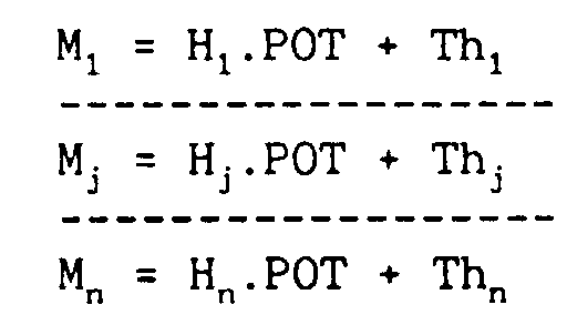
Les n combinaisons Mn peuvent être obtenues soit par une couche de n neurones comme cela vient d'être décrit, soit par plusieurs couches de neurones qui délivrent également n combinaisons. Ces potentiels neuronaux sont alors soumis à l'action de la fonction non linéaire CNLF.The n combinations M n can be obtained either by a layer of n neurons as has just been described, or by several layers of neurons which also deliver n combinations. These neural potentials are then subjected to the action of the non-linear function CNLF.
Les moyens 22 d'application de la fonction CNLF sont alors formés d'unités 351..., 35j..., 35n appliquant chacun préférentiellement une même fonction CNLF. Une unité 35n est constituée par exemple de deux comparateurs 361, 362 qui détectent lorsque Mn est respectivement supérieur ou égal à xmax et inférieur ou égal à -xmin. Une table 37 est alors adressée soit par les sorties des comparateurs 361, 362 lorsqu'ils sont actifs soit par Mn lorsque les comparateurs ne sont pas actifs. La table est préalablement chargée par les valeurs F(x), Fmax et -Fmin. Il est possible de n'utiliser qu'une seule unité 35 opérant successivement sur chaque potentiel M1,... Mj,... Mn.The means 22 for applying the CNLF function are then formed of units 35 1 ..., 35 d ..., 35 n each preferably applying the same CNLF function. A unit 35 n consists for example of two comparators 36 1 , 36 2 which detect when M n is respectively greater than or equal to x max and less than or equal to -x min . A table 37 is then addressed either by the outputs of the comparators 36 1 , 36 2 when they are active or by M n when the comparators are not active. The table is previously loaded with the values F (x), F max and -F min . It is possible to use only one unit 35 operating successively on each potential M 1 , ... M j , ... M n .
Des exemples de fonctions non linéaires CNLF sont représentés sur la figure 5. Hors de l'intervalle (-xmin, xmax) toutes les fonctions se stabilisent respectivement à -Fmin et Fmax. Les valeurs -Fmin et Fmax peuvent être quelconques mais constantes.Examples of non-linear CNLF functions are shown in Figure 5. Outside the interval (-x min , x max ) all functions stabilize at -F min and F max respectively . The values -F min and F max can be arbitrary but constant.
Dans l'intervalle (-xmin, xmax), la fonction F(x) peut être formée d'une rampe (courbe F1) ou d'un polynôme d'ordre 3 (courbe F2) ou d'une courbe plus complexe (courbe F3).In the interval (-x min , x max ), the function F (x) can be formed by a ramp (curve F1) or a polynomial of order 3 (curve F2) or a more complex curve (curve F3).
Préférentiellement selon l'invention, on utilise une rampe dans l'intervalle (-xmin, xmax). Cette fonction a en effet l'avantage de ne nécessiter que peu de moyens matériels. Elle a également un avantage supplémentaire, le calcul associé de sa dérivée ne nécessitant que peu de moyens supplémentaires.Preferably according to the invention, a ramp is used in the interval (-x min , x max ). This function has the advantage of requiring very little material means. It also has an additional advantage, the associated calculation of its derivative requiring only a few additional means.
La figure 6 représente un exemple de réalisation d'une unité 35, par exemple de l'unité 35n, dans le cas de la rampe pour la voie d'ordre n. Pour simplifier le schéma, les valeurs de Fmax et -Fmin sont normalisées respectivement à + 1 et - 1 ainsi que xmax et -xmin.FIG. 6 represents an exemplary embodiment of a unit 35, for example of the unit 35 n , in the case of the ramp for the way of order n. To simplify the diagram, the values of F max and -F min are normalized respectively to + 1 and - 1 as well as x max and -x min .
Le potentiel neuronal Mn entre dans deux comparateurs 361, 362 qui détectent respectivement lorsque Mn ≥ 1 et Mn ≤ - 1.The neural potential M n enters two comparators 36 1 , 36 2 which detect respectively when M n ≥ 1 and M n ≤ - 1.
Lorsque Mn ≥ 1, la sortie 611 est activée (état Y). Elle actionne alors un organe 63 qui force une valeur Fmax = + 1 sur la sortie Sn.When M n ≥ 1, output 61 1 is activated (state Y). It then actuates a
Lorsque Mn ≤ - 1, la sortie 621 est activée (état Y). Elle actionne alors un organe 67 qui force une valeur Fmin = - 1 sur la sortie Sn.When M n ≤ - 1, output 62 1 is activated (state Y). It then actuates a
Lorsque - 1 < Mn < + 1, les sorties 612 et 622 sont activées (état N). Elles entrent dans une porte ET 64 qui agit sur une porte de transfert 65 qui transfère chaque valeur Mn (bus 38) sur la sortie Sn. Il y a alors identité entre les potentiels neuronaux Mn et les états Sn.When - 1 <M n <+ 1, outputs 61 2 and 62 2 are activated (state N). They enter an AND
Toutes les unités 351 - 35n de la figure 4 sont identiques entre elles lorsque tous les potentiels Mj sont soumis à l'action de la même fonction F(x). Il est possible de choisir des fonctions F(x) différentes. Tous les états (S1 - Sn) arrivent, avec les coefficients synaptiques Dj, dans l'unité neuronale 24 (figure 4) qui effectue les calculs :
L'unité neuronale 24 est formée d'un seul neurone qui n'est pas nécessairement suivi par l'action d'une fonction d'activation.The
Les coefficients Hj et Dj stockés dans la mémoire 26 pour être utilisés respectivement dans les unités neuronales 20 et 24 doivent être prédéterminés en fonction du choix des fonctions non linéaires NLF, ANLF et CNLF utilisées et de l'erreur d'approximation tolérée. Dans le cas où CNLF est une rampe, la méthode de calcul est la suivante .The coefficients H j and D j stored in the
La fonction non linéaire ANLF, ayant pour équation A(x), est une approximation de la fonction non linéaire NLF, ayant pour équation T(x). Il est possible d'utiliser des critères différents pour définir la fonction ANLF :
- un premier critère peut consister à fixer a priori une erreur E qui ne doit pas être dépassée entre les fonctions NLF et ANLF,
- un second critère peut consister à fixer a priori le nombre de segments (donc de potentiels neuronaux Mj délivrés par l'unité neuronale 20) que l'on désire utiliser pour obtenir l'approximation de la fonction NLF.
- a first criterion may consist in fixing a priori an error E which must not be exceeded between the functions NLF and ANLF,
- a second criterion may consist in fixing a priori the number of segments (therefore of neural potentials M j delivered by the neural unit 20) that one wishes to use to obtain the approximation of the NLF function.
Selon le premier critère, à partir de l'abscisse xo = o (Figure 2), on fait passer une droite de pente po et on calcule l'abscisse x1 du point où cette droite rencontre la courbe de la fonction NLF en faisant que l'erreur maximale atteigne la valeur E entre le segment de droite et ladite courbe. On répète le calcul à partir du point x1 et ainsi de suite pour toute la courbe de la fonction NLF. Le calcul est arrêté lorsque l'erreur maximale devient inférieure à la valeur E. On dispose ainsi d'une suite de segments de droite définis par leur pente et leurs extrémités. L'équation d'un segment de droite d'ordre k, entre xk et xk+1, est :![]()
- pk :
- la pente
- qk :
- l'ordonnée à l'origine.
- p k :
- slope
- q k :
- the intercept.
Du fait que A(x) et T(x) coïncident aux extrémités des segments, on obtient :![]()
avec pn = o car le dernier segment a une pente nulle
et![]()
La fonction T(x) est supposée convexe (x ≥ o) et impaire. Le calcul concerne des valeurs x ≥ o.Because A (x) and T (x) coincide at the ends of the segments, we obtain: ![]()
with p n = o because the last segment has a zero slope
and ![]()
The function T (x) is assumed to be convex (x ≥ o) and odd. The calculation concerns values ≥ ≥ o.
L'erreur e k (x) entre les deux courbes T(x) et A(x) s'écrit:![]()
![]()
Le point x = x ![]()
e'(x) = o soit T'(x ![]()
![]()
e '(x) = o or T' (x ![]()
En prenant une fonction tangente hyperbolique pour T(x), on démontre que pour les segments à pente non nulle :![]()
![]()
En procédant successivement sur k croissant, en connaissant xk et en écrivant que e![]()
![]()
Selon le second critère, on fixe a priori un nombre de segments. On détermine alors les extrémités des segments pour que les erreurs maximales pour chaque segment, y compris pour le dernier segment, soient rigoureusement égales. La méthode de calcul qui vient d'être décrite pour le premier critère peut être légèrement adaptée pour traiter ce second critère. Cette démarche est à la portée de l'homme du métier.According to the second criterion, a number of segments are a priori fixed. The ends of the segments are then determined so that the maximum errors for each segment, including the last segment, are strictly equal. The calculation method which has just been described for the first criterion can be slightly adapted to deal with this second criterion. This approach is within the reach of those skilled in the art.
En fixant a priori soit la valeur E de l'erreur maximale admise soit le nombre de segments formant la fonction ANLF, il est possible de prédéterminer la précision de l'approximation.By setting a priori either the value E of the maximum accepted error or the number of segments forming the ANLF function, it is possible to predetermine the precision of the approximation.
Lorsque la fonction non linéaire d'approximation ANLF a été déterminée, il reste à calculer les coefficients synaptiques Hj et Dj avec 1 ≤ j ≤ n. Le nombre n de coefficients synaptiques est préférentiellement égal au nombre de segments à pente non nulle constituant la fonction ANLF dans le premier quadrant. En faisant correspondre les extrémités et les pentes des segments avec les coefficients Hj et Dj, dans le cas d'une rampe, un jeu de coefficients synaptiques possibles est :![]()
![]()
En effet, pour un segment d'ordre k, on peut écrire :
![]()
![]()
A titre d'exemple dans le cas d'une approximation d'une fonction tangente hyperbolique par 15 segments de droite avec une fonction non linéaire CNLF formée d'une rampe, on a calculé les coefficients synaptiques Hj et Dj suivants pour une précision à 10 chiffres significatifs :
La Table 1 représente les coefficients synaptiques Hj et la Table 2 représente les coefficients synaptiques Dj.Table 1 represents the synaptic coefficients H j and Table 2 represents the synaptic coefficients D j .
La méthode décrite précédemment est faite pour le cas où la fonction CNLF comprend une rampe. La méthode s'applique par analogie au cas où la fonction CNLF comprend non pas une rampe mais des parties de fonction plus complexes.The method described above is made for the case where the CNLF function comprises a ramp. The method applies by analogy to the case where the CNLF function does not include a ramp but more complex function parts.
Lors de l'utilisation du processeur neuronal 10, il peut être nécessaire de mettre en oeuvre des algorithmes d'apprentissage qui nécessitent de disposer de la dérivée de la fonction ANLF.When using the
Une première solution consiste alors à considérer cette dérivée comme une fonction nouvelle et à opérer son approximation comme cela vient d'être décrit jusqu'alors.A first solution then consists in considering this derivative as a new function and in operating its approximation as has just been described until now.
Une deuxième solution consiste à mettre à profit la mise en oeuvre utilisée pour la fonction ANLF afin de ne pas dupliquer inutilement certains moyens matériels et aussi de pas calculer une approximation de la dérivée de la fonction ANLF mais au contraire la dérivée première exacte de la fonction ANLF. La rampe constitue un cas particulièrement intéressant.A second solution consists in taking advantage of the implementation used for the ANLF function in order not to unnecessarily duplicate certain material means and also not to calculate an approximation of the derivative of the ANLF function but on the contrary the exact first derivative of the function ANLF. The ramp is a particularly interesting case.
Il a été décrit précédemment que :
La dérivée de la fonction ANLF revient à calculer la dérivée de STAT, c'est-à-dire :![]()
![]()
La dérivée de la fonction rampe R s'écrit :
- . lorsque POT ≤ - 1 ou POT ≥ 1 alors R'(.) = 0
- . et lorsque - 1 < POT < 1 alors R'(.) = 1.
- . when POT ≤ - 1 or POT ≥ 1 then R '(.) = 0
- . and when - 1 <POT <1 then R '(.) = 1.
En comparant les équations (1) et (2) précédentes, on constate alors que la différence entre les calculs de STAT(POT) et STAT'(POT) consiste à passer de la fonction rampe R à la fonction Hj.R'.By comparing the above equations (1) and (2), we can see that the difference between the calculations of STAT (POT) and STAT '(POT) consists in going from the ramp function R to the function H j .R'.
Le calcul de la dérivée peut donc être réalisé par une structure identique à celle de la figure 4, hormis les blocs 35 qui sont alors représentés sur la figure 7. Les potentiels neuronaux Mj, 1 ≤ j ≤ n, entrent dans les comparateurs 361, 362 qui détectent lorsque Mj ≥ 1 et lorsque Mj ≤ - 1. Les sorties 612 et 622 sont activées lorsque - 1 < Mj < 1. Ces sorties 612, 622 entrent dans la porte ET 64 qui active une porte de transfert 70 qui transfère le coefficient synaptique Hj correspondant au potentiel Mj d'indice j.The computation of the derivative can therefore be carried out by a structure identical to that of FIG. 4, except for the blocks 35 which are then represented in FIG. 7. The neuronal potentials M j , 1 ≤ j ≤ n, enter the comparators 36 1 , 36 2 which detect when M j ≥ 1 and when M j ≤ - 1. The outputs 61 2 and 62 2 are activated when - 1 <M j <1. These outputs 61 2 , 62 2 enter the gate AND 64 which activates a
Lorsque la condition - 1 < Mj < 1 n'est pas vérifiée, la porte ET 64 active un inverseur 72 qui commande un élément 71 qui force un signal nul sur la sortie Sj.When the condition - 1 <M j <1 is not verified, the AND
Les schémas des figures 6 et 7 peuvent être combinés (figure 8) pour être utilisés successivement soit pour le calcul de la fonction ANLF soit pour le calcul de sa dérivée. Pour cela, un signal de fonction FUNCT permet de sélectionner l'un ou l'autre mode.The diagrams in Figures 6 and 7 can be combined (Figure 8) to be used successively either for the calculation of the ANLF function or for the calculation of its derivative. To do this, a FUNCT function signal allows you to select one or the other mode.
Lorsque le signal FUNCT est activé, il active des portes ET 80, 82, 84 qui commandent les blocs 63, 65, 67 précédemment décrits.When the FUNCT signal is activated, it activates AND
Un signal FUNCT pas activé constitue alors une commande pour le calcul de la dérivée. Ce signal passe dans un inverseur 85 qui active des portes ET 81, 83 qui commandent les blocs 70, 71 précédemment décrits.A FUNCT signal not activated then constitutes a command for calculating the derivative. This signal passes through an
On dispose ainsi d'un bloc 35 compact qui permet de calculer soit la fonction ANLF soit la dérivée première exacte de la fonction ANLF. L'approximation faite de la fonction NLF par la fonction ANLF peut être obtenue avec une précision prédéterminée aussi grande que cela est désiré.There is thus a compact block 35 which makes it possible to calculate either the ANLF function or the exact first derivative of the ANLF function. The approximation of the NLF function by the ANLF function can be obtained with a predetermined precision as large as desired.
Il est possible de calculer la fonction dérivée selon une variante. Comme cela vient d'être décrit, la porte de transfert 70 (figures 7 et 8) sert à propager les valeurs des coefficients Hj. Il est possible d'obtenir un résultat identique en mettant l'entrée de la porte 70 à une valeur 1 et en multipliant les états Sj par les coefficients synaptiques Dj et par les coefficients synaptiques Hj (à j constant). Ceci est par exemple obtenu en stockant des coefficients synaptiques Dj.Hj dans la mémoire 26 (figure 3). Ainsi avantageusement l'architecture des blocs 22 n'est pas modifiée pour passer du calcul de la fonction F, avec les coefficients synaptiques Hj et Dj, au calcul de sa dérivée F', avec les coefficients synaptiques Hj et Dj.Hj.It is possible to calculate the derivative function according to a variant. As has just been described, the transfer gate 70 (FIGS. 7 and 8) serves to propagate the values of the coefficients H j . It is possible to obtain an identical result by setting the input of
L'autre processeur neuronal 14 représenté sur la figure 4 peut être formé de moyens matériels indépendants des autres moyens du processeur neuronal 10 (figure 1). Néanmoins, une solution avantageuse consiste à réaliser l'autre processeur neuronal 14 à partir de l'unité neuronale 12 et de la mémoire 16 du processeur neuronal 10. En effet, le calcul des potentiels neuronaux POT puis celui de l'application de la fonction d'activation forment des opérations séparées dans le temps. Des neurones de l'unité neuronale 12 peuvent donc dans un premier temps être affectés au calcul des potentiels neuronaux POT puis peuvent ensuite être affectés au calcul des états neuronaux STAT par application de la fonction non linéaire ANLF.The other
La construction d'une fonction non linéaire G, d'un degré élevé de complexité à partir de fonctions de base S d'un degré de complexité plus faible, est indiquée sur les figures 9 à 12 à titre d'exemple.The construction of a non-linear function G, of a high degree of complexity from basic functions S of a lower degree of complexity, is shown in Figures 9 to 12 by way of example.
Dans cet exemple, la fonction non linéaire G est supposée être une fonction non linéaire par morceaux consistant en une pluralité de segments de droite. La fonction G est de plus supposée être une approximation d'une fonction sigmoïde impaire habituellement mise en oeuvre dans le fonctionnement des réseaux de neurones. La fonction non linéaire G agit sur le potentiel neuronal POT. Le diagramme de la figure 9 illustre la partie positive de G, montrant qu'elle renferme quatre portions linéaires avec des cassures en A, B et C.In this example, the nonlinear function G is assumed to be a piecewise nonlinear function consisting of a plurality of line segments. The function G is moreover supposed to be an approximation of an odd sigmoid function usually implemented in the functioning of neural networks. The nonlinear function G acts on the POT neural potential. The diagram in Figure 9 illustrates the positive part of G, showing that it contains four linear portions with breaks in A, B and C.
Il est de plus considéré que les fonctions de base S suivantes sont disponibles :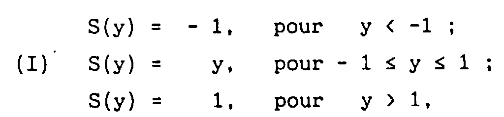
Premièrement, on crée trois fonctions linéaires Mj,
1 ≤ j ≤ 3 opérant sur POT.![]()
1 ≤ j ≤ 3 operating on POT. ![]()
Ceci est indiqué sur le diagramme de la figure 11. Les coefficients Hj sont constants et prédéterminés comme cela sera indiqué ci-après.This is indicated on the diagram in FIG. 11. The coefficients H j are constant and predetermined as will be indicated below.
Deuxièmemement, la fonction de base S agit sur chaque Mj pour produire un Sj, toujours en fonction de POT :![]()
![]()
![]()
![]()
Comme H1 > H2 > H3, on peut déduire les caractéristiques suivantes. Au-delà de POT = 1/Hj, la fonction de base S reste égale à l'unité. En d'autres mots, la contribution de Sj à G(POT) au-delà de cette valeur de POT, reste constante. Au-delà de POT = 1/H3, les contributions de Sj sont constantes. Pour 1/H2 ≤ POT ≤ 1/H3, les contributions de S1 et S2 sont constantes, tandis que S3 fournit à G une contribution variant linéairement. Pour 1/H1 ≤ POT ≤ 1/H2, les contributions de S2 et S3 varient linéairement, et S1 est constant. Pour 0 ≤ POT ≤ 1/H1, les contributions de S1, S2 et S3 varient linéairement.As H 1 > H 2 > H 3 , we can deduce the following characteristics. Beyond POT = 1 / H j , the basic function S remains equal to unity. In other words, the contribution of S j to G (POT) beyond this value of POT, remains constant. Beyond POT = 1 / H 3 , the contributions of S j are constant. For 1 / H 2 ≤ POT ≤ 1 / H 3 , the contributions of S 1 and S 2 are constant, while S 3 provides G with a linearly varying contribution. For 1 / H 1 ≤ POT ≤ 1 / H 2 , the contributions of S 2 and S 3 vary linearly, and S 1 is constant. For 0 ≤ POT ≤ 1 / H 1 , the contributions of S 1 , S 2 and S 3 vary linearly.
En conséquence, on obtient les équations suivantes :![]()
![]()
![]()
![]()
![]()
![]()
Comme les 1/Hj sont associés aux valeurs de POT où apparaissent les cassures (A, B et C), les Dj peuvent être aisément déterminés à partir de ce jeu de trois équations linéaires à trois inconnues.As the 1 / H j are associated with the POT values where the breaks appear (A, B and C), the D j can be easily determined from this set of three linear equations with three unknowns.
Ce qui vient d'être indiqué est qu'une combinaison convenable de fonctions de bases Sj d'un faible degré de complexité peuvent être utilisées pour créer une fonction non linéaire prédéterminée ayant un degré de complexité plus élevé.What has just been said is that a suitable combination of basic functions S j of a low degree of complexity can be used to create a predetermined nonlinear function having a higher degree of complexity.
La conséquence pratique est que les fonctions M et S peuvent aisément être implémentées en utilisant une très simple architecture de réseau de neurones de façon à fournir une possibilité de calcul de fonction non linéaire plus compliquée mise en oeuvre dans un réseau de neurones.The practical consequence is that the M and S functions can easily be implemented using a very simple neural network architecture so as to provide a more complicated nonlinear function calculation possibility implemented in a neural network.
Notons que la construction présentée d'une fonction non linéaire d'un degré élevé de complexité n'est pas limitée aux réseaux de neurones, mais peut également être appliquée au domaine des contrôleurs non linéaires qui utilisent des fonctions de transfert non linéaires comme opérations prépondérantes dans le chemin de données. A cette fin, le contrôleur non linéaire peut comprendre lui-même un réseau de neurones simple.Note that the presented construction of a non-linear function with a high degree of complexity is not limited to neural networks, but can also be applied to the field of non-linear controllers which use non-linear transfer functions as preponderant operations. in the data path. To this end, the nonlinear controller can itself include a simple neural network.
Claims (11)
- A data processing system, comprising means (14) for calculating on the basis of an input signal representing neural potentials (POT) which are to be subjected to a complex non-linear function (NLF), an output signal representing a neural state (STAT) by means of a segmented (or piecewise) non-linear functions (ANLF) approximating said non-linear function (NLF), characterized in that said means for transformation comprise:- first means (20) comprising a neural unit for calculating first combinations M1 - Mn of said input signal with first synaptic coefficients Hj,- second means (22) for subjecting the firs combinations (M1-Mn) to at least one other non-linear function (CNLF) which comprises a non-constant intermediate part F(x) and constant extreme parts (Fmax,-Fmin) and for supplying second combinations (S1 - SN),- third means (24) comprising a neural unit for calculating each segment by linear combination of the second segment (S1-Sn) by means of second synaptic coefficient (Dj) and for delivering the output signal
 - storage means (26) for storing said first and second synaptic coefficients (Hj, Dj).
 - A system as claimed in Claim 1, characterized in that the second means (22) comprise:- means (361, 362, 64) for detecting whether the first combinations have values associated with said intermediate part or not,- means (37) for applying the intermediate part of the non linear function to the first combinations when the first combinations have values associated with said intermediate part, and for attributing constant values to the second combinations when the first combinations have values associated with the extreme parts.
- A system as claimed in Claim 2, characterized in that the means (37) comprise a table which stores values of second combinations at addresses formed by the first combinations.
- A system as claimed in Claim 2, characterized in that the other non-linear function is a ramp, the means (37) being formed by transfer means (38, 65) which impose on the second combinations values which are either equal to or proportional to the first combinations.
- A system as claimed in any one of the Claims 1 to 4, characterized in that it also comprises means (75) for calculating a derivative of said non-linear function.
- A system as claimed in Claim 5, characterized in that the means (75) comprise at least one other table which stores predetermined values resulting from an application of a derivate of the other non-linear function to the first combinations when the first combinations have values associated with said intermediate part, and otherwise stores values zero.
- A system as claimed in Claim 6, characterized in that the other non-linear function is a ramp, the other table being replaced by a block (70) which performs the application of the derivative by copying said first coefficients.
- A system as claimed in one of the Claims 1 to 7, characterized in that the second means (22) are used for successively calculating applications according to the non-linear function and applications according to its derivative.
- A system as claimed in one of the Claims 1 to 8, characterized in that the input signal is a neural potential from a neural network, the segmented non-linear function being an approximation of a non-linear neural activation function.
- A system as claimed in Claim 9, characterized in that said means for transforming are implemented by means of another programmed neural network.
- A system as claimed in Claim 10, characterized in that the neurons of said neural network are successively programmed for forming the other neural network.
Applications Claiming Priority (2)
| Application Number | Priority Date | Filing Date | Title |
|---|---|---|---|
| FR9115373A FR2685109A1 (en) | 1991-12-11 | 1991-12-11 | NEURAL DIGITAL PROCESSOR OPERATING WITH APPROXIMATION OF NONLINEAR ACTIVATION FUNCTION. |
| FR9115373 | 1991-12-11 |
Publications (2)
| Publication Number | Publication Date |
|---|---|
| EP0546624A1 EP0546624A1 (en) | 1993-06-16 |
| EP0546624B1 true EP0546624B1 (en) | 1997-11-19 |
Family
ID=9419921
Family Applications (1)
| Application Number | Title | Priority Date | Filing Date |
|---|---|---|---|
| EP92203774A Expired - Lifetime EP0546624B1 (en) | 1991-12-11 | 1992-12-04 | Data processing system operating with non-linear function divided into pieces |
Country Status (5)
| Country | Link |
|---|---|
| US (1) | US5796925A (en) |
| EP (1) | EP0546624B1 (en) |
| JP (1) | JP3315449B2 (en) |
| DE (1) | DE69223221T2 (en) |
| FR (1) | FR2685109A1 (en) |
Families Citing this family (28)
| Publication number | Priority date | Publication date | Assignee | Title |
|---|---|---|---|---|
| EP0683462A3 (en) * | 1994-03-31 | 1996-01-17 | Philips Electronique Lab | Procedure and processor for constructing a piecewise linear function with eventual discontinuities. |
| FR2724027A1 (en) * | 1994-11-25 | 1996-03-01 | France Telecom | Neural operator for non-linear equalisers for television receivers |
| US7433097B2 (en) * | 2003-04-18 | 2008-10-07 | Hewlett-Packard Development Company, L.P. | Optical image scanner with moveable calibration target |
| DE102006046204B3 (en) * | 2006-09-29 | 2008-07-17 | Siemens Ag | Device for neuronal control or regulation in internal combustion engine, has piecewise parabolic function provided as activating function |
| US9477926B2 (en) | 2012-11-20 | 2016-10-25 | Qualcomm Incorporated | Piecewise linear neuron modeling |
| US10049326B1 (en) * | 2013-02-01 | 2018-08-14 | The United States of America as Represented by the Admin of National Aeronautics and Space Administration | Systems and methods for transfer function estimation using membership functions |
| EP2821183B1 (en) | 2013-07-05 | 2017-06-21 | Black & Decker Inc. | Hammer Drill |
| CN105893159B (en) * | 2016-06-21 | 2018-06-19 | 北京百度网讯科技有限公司 | Data processing method and device |
| JP2018092294A (en) * | 2016-12-01 | 2018-06-14 | ソニーセミコンダクタソリューションズ株式会社 | Computing device, computing method and computer program |
| US11544545B2 (en) | 2017-04-04 | 2023-01-03 | Hailo Technologies Ltd. | Structured activation based sparsity in an artificial neural network |
| US10387298B2 (en) | 2017-04-04 | 2019-08-20 | Hailo Technologies Ltd | Artificial neural network incorporating emphasis and focus techniques |
| US11615297B2 (en) | 2017-04-04 | 2023-03-28 | Hailo Technologies Ltd. | Structured weight based sparsity in an artificial neural network compiler |
| US11238334B2 (en) | 2017-04-04 | 2022-02-01 | Hailo Technologies Ltd. | System and method of input alignment for efficient vector operations in an artificial neural network |
| US11551028B2 (en) | 2017-04-04 | 2023-01-10 | Hailo Technologies Ltd. | Structured weight based sparsity in an artificial neural network |
| US10872290B2 (en) | 2017-09-21 | 2020-12-22 | Raytheon Company | Neural network processor with direct memory access and hardware acceleration circuits |
| US11468332B2 (en) | 2017-11-13 | 2022-10-11 | Raytheon Company | Deep neural network processor with interleaved backpropagation |
| US11522671B2 (en) | 2017-11-27 | 2022-12-06 | Mitsubishi Electric Corporation | Homomorphic inference device, homomorphic inference method, computer readable medium, and privacy-preserving information processing system |
| US11475305B2 (en) * | 2017-12-08 | 2022-10-18 | Advanced Micro Devices, Inc. | Activation function functional block for electronic devices |
| RU182699U1 (en) * | 2018-05-31 | 2018-08-28 | Федеральное государственное бюджетное образовательное учреждение высшего образования "МИРЭА - Российский технологический университет" | PULSE BLOCK OF CALCULATION OF ACTIVATION FUNCTION OF AN ARTIFICIAL NEURAL NETWORK |
| US11775805B2 (en) * | 2018-06-29 | 2023-10-03 | Intel Coroporation | Deep neural network architecture using piecewise linear approximation |
| CN110688088B (en) * | 2019-09-30 | 2023-03-28 | 南京大学 | General nonlinear activation function computing device and method for neural network |
| US11263077B1 (en) | 2020-09-29 | 2022-03-01 | Hailo Technologies Ltd. | Neural network intermediate results safety mechanism in an artificial neural network processor |
| US11237894B1 (en) | 2020-09-29 | 2022-02-01 | Hailo Technologies Ltd. | Layer control unit instruction addressing safety mechanism in an artificial neural network processor |
| US11221929B1 (en) | 2020-09-29 | 2022-01-11 | Hailo Technologies Ltd. | Data stream fault detection mechanism in an artificial neural network processor |
| US11811421B2 (en) | 2020-09-29 | 2023-11-07 | Hailo Technologies Ltd. | Weights safety mechanism in an artificial neural network processor |
| US11874900B2 (en) | 2020-09-29 | 2024-01-16 | Hailo Technologies Ltd. | Cluster interlayer safety mechanism in an artificial neural network processor |
| CN113935480B (en) * | 2021-11-12 | 2022-10-18 | 成都甄识科技有限公司 | Activation function acceleration processing unit for neural network online learning |
| KR102651560B1 (en) * | 2021-12-01 | 2024-03-26 | 주식회사 딥엑스 | Neural processing unit including a programmed activation functrion execution unit |
Family Cites Families (15)
| Publication number | Priority date | Publication date | Assignee | Title |
|---|---|---|---|---|
| US3601811A (en) * | 1967-12-18 | 1971-08-24 | Matsushita Electric Ind Co Ltd | Learning machine |
| FR2625347B1 (en) * | 1987-12-23 | 1990-05-04 | Labo Electronique Physique | NEURON NETWORK STRUCTURE AND CIRCUIT AND ARRANGEMENT OF NEURON NETWORKS |
| US4979126A (en) * | 1988-03-30 | 1990-12-18 | Ai Ware Incorporated | Neural network with non-linear transformations |
| DE68928385T2 (en) * | 1988-08-31 | 1998-02-12 | Fujitsu Ltd | NEURONIC CALCULATOR |
| FR2639739B1 (en) * | 1988-11-25 | 1991-03-15 | Labo Electronique Physique | METHOD AND DEVICE FOR COMPRESSING IMAGE DATA USING A NEURON NETWORK |
| FR2639736B1 (en) * | 1988-11-25 | 1991-03-15 | Labo Electronique Physique | GRADIENT BACKPROPAGATION METHOD AND NEURON NETWORK STRUCTURE |
| US5293459A (en) * | 1988-12-23 | 1994-03-08 | U.S. Philips Corporation | Neural integrated circuit comprising learning means |
| US5107442A (en) * | 1989-01-12 | 1992-04-21 | Recognition Equipment Incorporated | Adaptive neural network image processing system |
| FR2648253B1 (en) * | 1989-06-09 | 1991-09-13 | Labo Electronique Physique | TREATMENT METHOD AND NEURON NETWORK STRUCTURE IMPLEMENTING THE METHOD |
| US5109351A (en) * | 1989-08-21 | 1992-04-28 | Texas Instruments Incorporated | Learning device and method |
| GB2236608B (en) * | 1989-10-06 | 1993-08-18 | British Telecomm | Digital neural networks |
| US5067095A (en) * | 1990-01-09 | 1991-11-19 | Motorola Inc. | Spann: sequence processing artificial neural network |
| JP2785155B2 (en) * | 1990-09-10 | 1998-08-13 | 富士通株式会社 | Asynchronous control method for neurocomputer |
| US5097141A (en) * | 1990-12-12 | 1992-03-17 | Motorola, Inc. | Simple distance neuron |
| US5228113A (en) * | 1991-06-17 | 1993-07-13 | The United States Of America As Represented By The Administrator Of The National Aeronautics And Space Administration | Accelerated training apparatus for back propagation networks |
-
1991
- 1991-12-11 FR FR9115373A patent/FR2685109A1/en not_active Withdrawn
-
1992
- 1992-12-04 EP EP92203774A patent/EP0546624B1/en not_active Expired - Lifetime
- 1992-12-04 DE DE69223221T patent/DE69223221T2/en not_active Expired - Fee Related
- 1992-12-08 JP JP32792492A patent/JP3315449B2/en not_active Expired - Fee Related
-
1995
- 1995-02-06 US US08/384,191 patent/US5796925A/en not_active Expired - Fee Related
Also Published As
| Publication number | Publication date |
|---|---|
| JP3315449B2 (en) | 2002-08-19 |
| FR2685109A1 (en) | 1993-06-18 |
| DE69223221D1 (en) | 1998-01-02 |
| JPH05242068A (en) | 1993-09-21 |
| EP0546624A1 (en) | 1993-06-16 |
| DE69223221T2 (en) | 1998-05-14 |
| US5796925A (en) | 1998-08-18 |
Similar Documents
| Publication | Publication Date | Title |
|---|---|---|
| EP0546624B1 (en) | Data processing system operating with non-linear function divided into pieces | |
| EP0624847B1 (en) | Device and method to generate an approximating function | |
| EP0521548B1 (en) | Neural network device and method for data classification | |
| EP0322966B1 (en) | Neural network circuit and structure | |
| EP0552074B1 (en) | Multiprocessor data processing system | |
| EP0198729B1 (en) | Electronic circuit simulation system | |
| EP0446084A1 (en) | Classification method in a hierarchized neural network | |
| EP0454535B1 (en) | Neural classification system and method | |
| EP0875032B1 (en) | Learning method generating small size neurons for data classification | |
| EP0729037B1 (en) | System for estimating received signals in the form of mixed signals | |
| EP0449353A1 (en) | Information processing device and method to select words contained in a dictionary | |
| WO2019020384A1 (en) | Computer for spiking neural network with maximum aggregation | |
| EP0568146B1 (en) | Neural processor with data normalising means | |
| EP0446974A1 (en) | Classification method for multiclass classification in a layered neural network and method-based neural network | |
| EP0401927B1 (en) | Learning method, neural network and computer for simulating said neural network | |
| EP3712775A1 (en) | Method and device for determining the overall memory size of an overall memory area allocated to data from a neural network in view of its topology | |
| WO2022171632A1 (en) | Neuromorphic circuit and associated training method | |
| FR2681709A1 (en) | INTERNAL CONNECTION METHOD FOR NEURON NETWORKS. | |
| EP3663989A1 (en) | Method and device for reducing the calculation load of a microprocessor designed to process data by a convolutional neural network | |
| EP3971785A1 (en) | Electronic computer for implementing an artificial neural network, with several types of blocks for calculating | |
| FR2655444A1 (en) | NEURONAL NETWORK WITH ELECTRONIC NEURONAL CIRCUITS WITH COEFFICIENT LEARNING AND METHOD OF LEARNING. | |
| EP4202770A1 (en) | Neural network with on-the-fly generation of network parameters | |
| EP0681246A1 (en) | Method and apparatus for the extraction of a subset of objects by optimizing a measure, using a neural network | |
| EP4187445A1 (en) | Method for learning synaptic weight values of a neural network, data processing method, associated computer program, calculator and processing system | |
| FR2648253A1 (en) | PROCESSING METHOD AND NETWORK STRUCTURE OF NEURONS USING THE METHOD |
Legal Events
| Date | Code | Title | Description |
|---|---|---|---|
| PUAI | Public reference made under article 153(3) epc to a published international application that has entered the european phase |
Free format text: ORIGINAL CODE: 0009012 |
|
| AK | Designated contracting states |
Kind code of ref document: A1 Designated state(s): DE FR GB |
|
| 17P | Request for examination filed |
Effective date: 19931213 |
|
| RAP1 | Party data changed (applicant data changed or rights of an application transferred) |
Owner name: PHILIPS ELECTRONICS N.V. Owner name: LABORATOIRES D'ELECTRONIQUE PHILIPS S.A.S. |
|
| GRAG | Despatch of communication of intention to grant |
Free format text: ORIGINAL CODE: EPIDOS AGRA |
|
| 17Q | First examination report despatched |
Effective date: 19970204 |
|
| GRAH | Despatch of communication of intention to grant a patent |
Free format text: ORIGINAL CODE: EPIDOS IGRA |
|
| GRAH | Despatch of communication of intention to grant a patent |
Free format text: ORIGINAL CODE: EPIDOS IGRA |
|
| GRAA | (expected) grant |
Free format text: ORIGINAL CODE: 0009210 |
|
| AK | Designated contracting states |
Kind code of ref document: B1 Designated state(s): DE FR GB |
|
| REF | Corresponds to: |
Ref document number: 69223221 Country of ref document: DE Date of ref document: 19980102 |
|
| GBT | Gb: translation of ep patent filed (gb section 77(6)(a)/1977) |
Effective date: 19980205 |
|
| RAP4 | Party data changed (patent owner data changed or rights of a patent transferred) |
Owner name: KONINKLIJKE PHILIPS ELECTRONICS N.V. Owner name: LABORATOIRES D'ELECTRONIQUE PHILIPS S.A.S. |
|
| PLBE | No opposition filed within time limit |
Free format text: ORIGINAL CODE: 0009261 |
|
| STAA | Information on the status of an ep patent application or granted ep patent |
Free format text: STATUS: NO OPPOSITION FILED WITHIN TIME LIMIT |
|
| 26N | No opposition filed | ||
| REG | Reference to a national code |
Ref country code: FR Ref legal event code: TP |
|
| REG | Reference to a national code |
Ref country code: GB Ref legal event code: IF02 |
|
| PGFP | Annual fee paid to national office [announced via postgrant information from national office to epo] |
Ref country code: FR Payment date: 20021223 Year of fee payment: 11 |
|
| PGFP | Annual fee paid to national office [announced via postgrant information from national office to epo] |
Ref country code: GB Payment date: 20021224 Year of fee payment: 11 |
|
| PGFP | Annual fee paid to national office [announced via postgrant information from national office to epo] |
Ref country code: DE Payment date: 20030217 Year of fee payment: 11 |
|
| PG25 | Lapsed in a contracting state [announced via postgrant information from national office to epo] |
Ref country code: GB Free format text: LAPSE BECAUSE OF NON-PAYMENT OF DUE FEES Effective date: 20031204 |
|
| PG25 | Lapsed in a contracting state [announced via postgrant information from national office to epo] |
Ref country code: DE Free format text: LAPSE BECAUSE OF NON-PAYMENT OF DUE FEES Effective date: 20040701 |
|
| GBPC | Gb: european patent ceased through non-payment of renewal fee |
Effective date: 20031204 |
|
| PG25 | Lapsed in a contracting state [announced via postgrant information from national office to epo] |
Ref country code: FR Free format text: LAPSE BECAUSE OF NON-PAYMENT OF DUE FEES Effective date: 20040831 |
|
| REG | Reference to a national code |
Ref country code: FR Ref legal event code: ST |