EP0449169A2 - Adaptive control system - Google Patents
Adaptive control system Download PDFInfo
- Publication number
- EP0449169A2 EP0449169A2 EP91104658A EP91104658A EP0449169A2 EP 0449169 A2 EP0449169 A2 EP 0449169A2 EP 91104658 A EP91104658 A EP 91104658A EP 91104658 A EP91104658 A EP 91104658A EP 0449169 A2 EP0449169 A2 EP 0449169A2
- Authority
- EP
- European Patent Office
- Prior art keywords
- output
- error
- input
- vector
- matrix
- Prior art date
- Legal status (The legal status is an assumption and is not a legal conclusion. Google has not performed a legal analysis and makes no representation as to the accuracy of the status listed.)
- Withdrawn
Links
Images


Classifications
-
- G—PHYSICS
- G05—CONTROLLING; REGULATING
- G05B—CONTROL OR REGULATING SYSTEMS IN GENERAL; FUNCTIONAL ELEMENTS OF SUCH SYSTEMS; MONITORING OR TESTING ARRANGEMENTS FOR SUCH SYSTEMS OR ELEMENTS
- G05B13/00—Adaptive control systems, i.e. systems automatically adjusting themselves to have a performance which is optimum according to some preassigned criterion
- G05B13/02—Adaptive control systems, i.e. systems automatically adjusting themselves to have a performance which is optimum according to some preassigned criterion electric
- G05B13/0205—Adaptive control systems, i.e. systems automatically adjusting themselves to have a performance which is optimum according to some preassigned criterion electric not using a model or a simulator of the controlled system
- G05B13/0255—Adaptive control systems, i.e. systems automatically adjusting themselves to have a performance which is optimum according to some preassigned criterion electric not using a model or a simulator of the controlled system the criterion being a time-optimal performance criterion
Definitions
- the present invention relates to an adaptive control system for controlling a physical plant such as a servo motor or a heat pump of which dynamic property can not be estimated and/or extraneous disturbance can not be disregarded.
- the error is defined by a difference between the output of the physical plant and a "desired trajectory" or the output of a reference model which are defined by a function of time with respect to the physical plant having an unknown property.
- the "desired trajectory” is defined by an aggregation of data which are given by a function of time and is a target of control in a physical plant. The aggregation of the data is distributed on a trajectory and hence is called the "desired trajectory”.
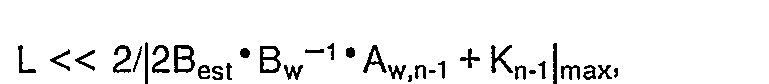
- the value of an input distribution matrix "B" estimated in advance is calculated by dividing the variation of the differential value of the output by the variation of an input thereof. Then, in the TDC, unknown dynamic property other than the input distribution matrix "B” is estimated by using a control input matrix "Best", the input value at a predetermined time length "L” ago and the differential value of the output at the predetermined time length "L” ago. The dispersion of the estimated value of the input distribution matrix "B” is canceled in the control input matrix "Best". Moreover, error characteristic of the TDC is adjusted by using an error dynamics adjustment matrix "K i ". The control input matrix "Best", time length "L” and error dynamic adjustment matrix "K;” are called “design parameters”.
- control input matrix "Best” having a high accuracy is not realizable in rapid variation of the input distribution matrix "B".
- the physical plant does not follow the desired trajectory, and in a worst case the TDC becomes unstable in the event that the input distribution matrix "B" is unknown.
- An object of the present invention is to provide an adaptive control system in which a control input matrix "Best" and design parameters can be determined so that the output of a physical plant follows a desired trajectory with stable and excellent following-property in the physical plant of multi-input-multi-output having an unknown input distribution matrix "B".
- an input distribution matrix "B” In a physical plant which is represented by a known “state space dynamics equation” given by the function B(t) of time is called an input distribution matrix "B" and represents characteristics of the control system described by the above-mentioned state space dynamics equation.
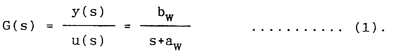
- a "first order lag system" of the single-input-single-output is simply represented by transfer function (1) as below:
- An input distribution matrix "B” is represented by an input distribution coefficient "b w " in transfer function form.
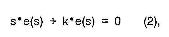
- a control input u(t) which satisfies the equation (2) is calculated by equation (3) (see USP 497257 of the prior art), where, k: error dynamics adjustment coefficient, L: a time length of a periodic time of control, for example, and "y" represents a differential value of "y".
- a control input matrix in the physical plant of multi-input-multi-output is represented by "Best", and a control input matrix in the physical plant of single-input-single-output is represented by “best”.
- Suffix "est” represents estimation value.
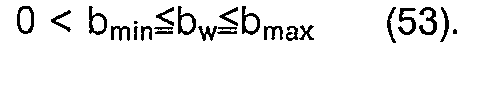
- variable ranges of the equation (1) is given by
- condition of stability is to be a negative value in the real part of a pole of the equation (13), and thus the condition of stability is given by
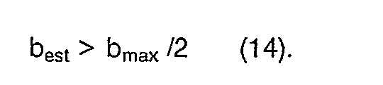
- the relation (14) is applied to the physical plant of single-input-single-output.
- m o a desired frequency range for the following-property.
- ordinate is graduated by the time length "L” and abscissa is graduated by the ratio of the control input coefficient "best" to the input distribution coefficient "b".
- control input matrix "Best” selection of the control input matrix "Best” is elucidated in detail with respect to the physical plant of two-input-two-output.
- An input distribution matrix "B w " and a control input matrix “Best” are defined by equations (31) and (32), respectively.
- the equation (27) is a quadratic expression of "s" in the event of two-input-two-output, and both relations (34) and (35) must be satisfied on the basis of the relations (28-1) --- (28-q) as a "necessary and sufficient condition of stability.
- the time length "L” of two-input-two-output is calculated by substituting the control input matrix "Best”tor the relations (22) --- (25), (29) and (30), and the time length "L" having the minimum value is selected.
- every components of the control input matrix "Best” are selected in a manner that "det(B est )" increases. Then, if the relations (28-1) --- (28-q) are not satisfied, every components of the control input matrix "Best” are changed in a manner that "det(B est )" increases.
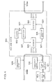
- FIG.1 is a perspective view of a servo motor system 106 of a physical plant to which a first embodiment of the adaptive control system in accordance with the present invention is applied.
- a shaft 101 is rotated by a servo motor 100.
- a rod 102 is affixed on the shaft 101 and is arranged perpendicularly with respect to the revolution axis of the shaft 101.
- a load 105 is supported on the rod 102 and is movable along the rod 102 as shown by arrow A.
- the load 105 is connected to a stationary member 107 with intermediates of a damper 103 having viscid material therein and a spring 105.
- the load 105 receives a resistant force from the damper 103 and spring 104 by movement of the rod 102 in the direction shown by arrow B and by movement of the load 105 in the direction shown by arrow A.
- a “viscous resistance” of the damper is represented by “c”
- a “spring constant” of the spring 104 is represented by “K s ".
- the rod 102 comprises a linear motor means, for example, and the load 105 is movable along the rod 102 during revolution of the shaft 101, the inertia of the motor system 106 is unknown.
- the revolution angle of the shaft 101 is represented by "y(t)"
- the input torque thereof is represented by "u(t)”.
- a differential equation for representing the action of the physical plant is given by
- the equation (50) represents a transfer function G(s) in the event that an input distribution coefficient "b w " is unknown and is varied.
- variable range of unknown characteristic "a W,i" and the input distribution coefficient "b w " are given by
- FIG.2 The block diagram of the adaptive control system of the first embodiment is shown in FIG.2.
- a physical plant 200 corresponds to the motor system 106 shown in FIG.1.
- the revolution angle, angular velocity and angular acceleration of the physical plant 200 are detected by an output sensor 201 comprising an encoder, a tachometer, an acceleration sensor and a processing circuit therefor.
- An arbitrary desired trajectory y d (t) of the angular acceleration of the function of time, differential values y d (t) and y d (t) of the desired trajectory y d (t) are output from a trajectory production means 202.
- the desired trajectory y d (t) and the differential value y d (t) of the desired trajectory y d (t) are applied to an error value production means 203.
- an output y(t) output from the state output detection means 201 and the differential value y(t) of the output y(t) are also applied to the error value production means 203, and calculation is performed on the basis of the equation (54). Consequently, en error e(t) and the differential value e(t) of the error e(t) are output therefrom.
- the error e(t), the differential value e(t) and the second order differential value y d (t) of the output of the trajectory production means 202 are applied to an input calculation means 204.
- an angle acceleration y(t-L) of the output of the state output detection means 201 which has detected a predetermined time length "L" ago is also inputted to the input calculation means 204.
- calculation is performed on the basis of equation (55) by using an input u(t-L) which has inputted the time length "L” ago. Consequently, a control input u(t) is output therefrom.
- control input coefficient "best” is selected to satisfy the relation (14) as following equation (57):
- the frequency band required for following-property of the desired trajectory is represented by "w o”
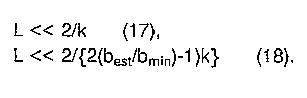
- the time length "L” is selected to satisfy the following entire relations:
- control input u(t) is converted into an input torque U(t) by a control input production means 205 which comprises an actuator or a driving circuit therefor, and is applied to the physical plant 200.
- control input production means 205 which comprises an actuator or a driving circuit therefor, and is applied to the physical plant 200.
- the output y(t) of the physical plant 200 which is produced by the applied input torque U(t) is controlled to confirm the desired trajectory.
- the control input therefor is calculated by the input calculation means 204 on the basis of the control input coefficient "best" and the time length "L", and hence the physical plant having unknown input distribution coefficient is made to follow the predetermined desired trajectory.
- FIG.3 is a graph representing relation between the time length "L" and the ratio of the control input coefficient "best” to the input distribution coefficient "b".
- An unstable area and a bad following-property area are illustrated by shaded areas, and a stable and good following-property area is illustrated by nonshaded area.
- a second embodiment of the adaptive control system in accordance with the present invention is to be applied to the physical plant of two-input-two-output having unknown input distribution matrix.
- a heat pump system is taken as an example of the physical plant.
- FIG.4 is a block diagram of the heat pump system 506, and FIG.5 is a block diagram of the adaptive control system for controlling the heat control system 506.
- a compressor 501, a condenser 503, an expansion valve 505 and an evaporator 500 are coupled in loop-shape by four pipe lines 507, and refrigerant is circulated through these pipe lines 507.
- a water line 508A is arranged adjacent to the evaporator 500, and the refrigerant is given heat from the water flowing the water line 508A.
- the refrigerant is compressed by the compressor 501 which is driven by an inverter 502.
- the compressed refrigerant is flowed in the condenser 503.
- Another water line 508B is arranged adjacent to the condenser 503, and the flow rate of the water is controlled by a water pump 504.
- heat of the refrigerant is given to the water flowing the water line 508B.
- the refrigerant is returned to the evaporator 500 through an expansion valve 505.
- FIG.5 is a block diagram of the adaptive control system of the second embodiment.
- a physical plant 600 in FIG.5 corresponds to the heat pump system 506 of FIG.4.
- a state output detection means 601 comprises a temperature sensor 509 for detecting temperature of the water at an outlet, a temperature sensor 510 for detecting temperature of water at an inlet thereof and a flow rate sensor 511.
- a temperature To( ⁇ C) which is a first output y 1 is detected by the temperature sensor 509.
- a temperature T in (°C) is detected by the temperature sensor 510.
- a temperature difference Tsub( C) is calculated by subtracting the temperature T in from the temperature To.
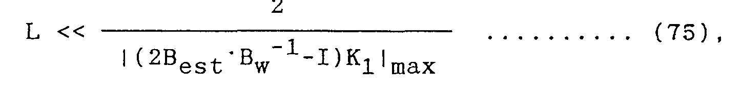
- control input matrix "Best" is the value given by Moreover, the time length L as the design parameter is determined so as to consistent with entire relations (74), (75), (76), (77), (78) and (79).
- control input vector u(t) which is output from the input calculation means 604 is converted into an input vector "U(t)" by a control input production means 605 which comprises an actuator and a driving circuit therefor and is applied to the physical plant 600.
- control input production means 605 which comprises an actuator and a driving circuit therefor and is applied to the physical plant 600.
- the output "y(t)" of the physical plant 600 is controlled to follow the desired trajectory in compliance with the input vector "U(t)".
- the output of the physical plant of two-input-two-output is controlled to follow the desired trajectory by using the control input matrix "Best" and the time length "L".
- the output of the physical plant having unknown input distribution matrix "B" is made to follow the desired trajectory.
- the physical plant having multi-input-multi-output can be controlled by using design parameters which satisfy the relations (28-1 )--(28-q) with respect to the control input matrix "Best", and by using the relations (22)--(25), (29) and (30) with respect to the time length L, and a similar effect is realizable.
- the time length "L” is selected in advance, and then the error dynamic adjustment matrix "K i " can be determined so as to satisfy the time length "L" selected in advance. Hence a similar result is realizable.
- a control input coefficient "best" is changed during operation of the adaptive control system so as to approach an actual input distribution coefficient "b". Consequently, the following-property of the output of a physical plant is further improved.
- the time length "L” is set to the value as mentioned in the second embodiment (relations (74)---(79)). Then, the initial value of a control input coefficient "best” is set to the control input coefficient "b max " so as to maintain stability with respect to variation of an input distribution coefficient "b". In the event that the following-property is not satisfied by the above-mentioned operation, the control input coefficient "best” is varied in a manner that the following-property is improved. The above-mentioned operation is described in detail below.
- the error is a time-variant value. Therefore, in the event that the conditions shown by the relations (80), (81) and (82) are not satisfied owing to the variation of the error, a time length T iim for satisfying the condition of the relation (80), for example, is detected during the set-time length t lim . Then, the ratio (r lim ) of the time length T,; m to the set-time length t lim is calculated as shown by relation (83), and the ratio (r lim ) can be used to determine the following-property.
- An average values of the error and the differential value of the error are usable as replacements for the error and the differential value of the error, and an example thereof is given by (II)
- a stability is determined to be bad.
- the product value of n-order differential value at a time (t) and at a time (t-L) is compared with a predetermined value (fed) of error as shown by relation (86).
- a product of differential values of inputs at the time (t) and at the (t-L) is compared with a predetermined value f ud of error as shown by relation (87). Referring to the relation (86) or (87), comparison is performed during the time length t lim or more.
- Design parameters can be changed in order to improve the following-property and stability as described below.
- a control input coefficient "best” is reduced at a predetermined rate by multiplying a control input coefficient "best” by a predetermined constant Cd which is smaller than "1.0” as shown by equation (88). Then, the control input coefficient "best” is calculated in accordance with an error as shown by non-linear relation (89) or (90). In this case, the control input coefficient "best” is reduced.
- "f a " and "f b " are constants which are given by the grade of error variation. When the constant "f b " is equal to "1.0", the relations (89) and (90) become linear relations.
- ave ) during the setting time t lim is usable as replacement for the absolute value of an error (
- control input coefficient "best” in the equation (90) is made to the control input coefficient "b max " as shown by equation (92).
- the control input coefficient "best" of the left sides is a new control input coefficient "best” which is calculated on the basis of an old control input coefficient "best” of the right sides.
- control input coefficient "best” is progressively reduced apart from an initial value of the control input coefficient ("b max ", for example) by the calculation of the relations (88) and (89). Consequently, the control input coefficient "best” approaches an optimum control input coefficient "bi ". Consequently, the error decreases, and thus the following-property is improved.
- the above-mentioned method is applicable to a physical plant of which the control input coefficient "b" is temporarily varied. Such case is shown, in FIG.1, in the example that the load 105 is moved along the rod 102 to a predetermined position, and after then the load 105 is held at the position.
- control input coefficient "b” is quickly varied, the variation method shown by equations (90) and (92) are preferable. Referring to the equations (90) and (92), the control input coefficient "best” is varied when the error is large, and in this case, the control input coefficient "best” is made to the control input coefficient "b max ".
- the control input coefficient "best” is made to increase at a constant rate by multiplying the input coefficient "best” by a predetermined constant C u which is larger than 1.0 as shown by the relation (93).
- control input coefficient "best” can be made to the control input coefficient "b max " as shown by relation (94).
- Calculations by the relations (80) --- (87) can be performed by fuzzy inference calculation.
- the situation part comprise variables for determining following-property
- the action part comprises variables for varying design parameters.
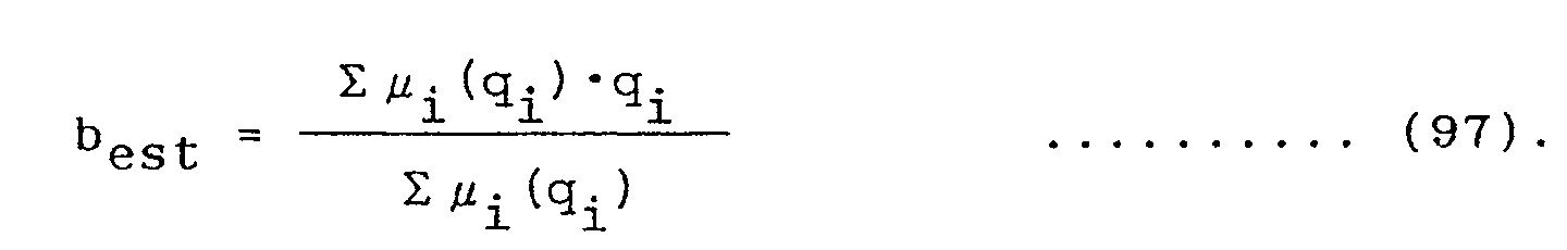
- fuzzy inference representation is given by where, PB: positive big, NS: negative small, q;: a real number.
- the fuzzy inference calculation comprises a plurality of the fuzzy inference representations. Consequently, the final result of the fuzzy inference calculation is given by
- the optimum design parameter can be obtained by an experimental method.
- the control input coefficient "best" of the TDC as shown by the equation (3), error dynamics adjustment matrix "k i " and time length "L" are automatically varied.
- FIG.7 is a graph of the relation between the time length "L” and the ratio of the control input coefficient "best” to the input distribution coefficient "b” for illustrating the areas of stability and following-property of an actual physical plant of single-input-single-output.
- ordinate is graduated by the time length "L”
- abscissa is graduated by the ratio of the control input coefficient "best” to the control input distribution coefficient "b”.
- An unstable area Q is produced by a parasitic mode such as the dead-time or the higher order dynamic characteristic.
- the stable-and-good-following-property area is liable to be narrowed. Furthermore, there is occasion where the design parameters lack the proper stable-and-good-following-property area.
- time length "L” is reduced, the following-property is improved.
- excessive reduction of the time length "L” results in oscillation of the adaptive control system in the event that the influence of the higher order dynamic characteristic or the dead-time can not be disregarded.
- the dynamics adjustment coefficient "k i " is decreased.
- the time length "L" is increased. Consequently, the stability is improved by the above-mentioned change of the design parameters.
- the error or the differential value of the error of the actual input distribution coefficient "b" are determined with respect to the physical plant of single-input-single-output by change of the control input coefficient "best” on the basis of the error, the differential value of the error or the differential value of the input. Then, the control input coefficient "best” is changed in real time, and thereby the output of the physical plant is made to follow the desired trajectory.
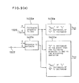
- FIG.8 is a block diagram of the third embodiment of the adaptive control system.
- the physical plant 200, the state output detection means 201, the trajectory production means 202, the error value production means 203 and the control production means 205 are identical with those of the first embodiment.
- following-property is determined by using the error e(t), in the event that the absolute value of the error is larger than a predetermined value f i as shown by relation (98).
- the control input coefficient "best” is not output by the second parameter change means 1309. Then the control input coefficient "best” which is output from the second parameter change means 1309 has priority to the control input coefficient "best” output from the first parameter change means 1308. The priority is determined by the parameter determination means 1310. Then, in the event that the control input coefficient "best” is output from the second parameter change means 1309, the control input coefficient "best” is employed by the parameter determination means 1310. On the other hand, in the event that the control input coefficient "best” is not output from the second parameter change means 1309, the control input coefficient "best" output from the first parameter change means 1308 is employed by the parameter determination means 1310.
- a control input u(t) is calculated by equation (103) in an input calculation means 1304 by using the control input coefficient "best" output from the parameter determination means 1310.
- the time length "L” is set to a value which satisfies the relations (58) --- (63) in a similar manner of the first embodiment. Moreover, the initial value of the control input coefficient "best” is set to the control input coefficient "b max " as given by the equation (57).
- the control input u(t) is applied to the physical plant 200 through the control input production means 205.
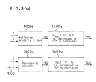
- FIGs. 9(a), 9(b), 9(c), 9(d) and 9(e) are block diagrams of relevant parts of the third embodiment for partially changing the configuration in FIG.8.
- a first and a second output judgment means 1406(a) and 1407(a) correspond to the first and second output judgment means 1306 and 1307 in FIG.8, respectively.
- a first and a second parameter change means 1408(a) and 1409(a) correspond to the first and second parameter change means 1308 and 1309 in FIG.8, respectively.
- the first output judgment means 1406(b) is comprised as replacement for the first output judgment means 1306, thereby calculation based on the relation (83) is performed.
- the ratio of a predetermined setting time t lim to a time length Turn in which the error value "e” exceeds a predetermined error value "f i " during the setting time tnm is obtained.
- the ratio is larger than a predetermined value rnm, bad following-property is determined. Then, stable control is realizable by increasing the setting-time t lim , and hence stable control is realizable.
- a first parameter change means 1408(c) shown in FIG.9(c) is used as replacement for the first parameter change means 1308 in FIG.8.
- calculation based on the equation (90) or equation (92) is performed in accordance with the output of the first output judgment means 1306 which is inputted to the first parameter change means 1408(c). Namely, in the event that the output of the first judgment means 1306 is "Yes” (the error value is larger than a predetermined value), the calculation of the equation (90) is performed, and the control input coefficient "best” is varied in accordance with the error value. On the other hand, in the event that the output of the first output judgment means 1306 is "No" (the error value is smaller than the predetermined value), the control input coefficient "b max " which is a maximum control input coefficient is employed.
- FIG.9(d) is a block diagram of an example using fuzzy inference calculation in a first output judgment means 1406(d) and a second parameter change means 1408(d).
- the fuzzy inference calculation five fuzzy variables of NB (negative big), NS (negative small), ZO (zero), PS (positive small), and PB (positive big) are set in the first output judgment means 1406(d).
- Data of an error "e” and the differential value “e” of the error “e” are memorized with a predetermined normalizing coefficient.
- the real values "q;” are selected in accordance with the fuzzy variables of the error “e” and the differential value “e” of the error “e” as shown in a table of the second parameter change means 1408(d).
- the normalizing coefficient and the real value "q i " are selected in a manner that the following property is improved.
- a first and second output judgment means 1406(e) and 1407(e) are used as replacements for the first and second output judgment means 1306 and 1307, respectively.
- a first and a second parameter change means 1408(e) and 1409(e) are used as replacements for the first and second parameter change means 1308 and 1309, respectively.
- the design parameters of the control input coefficient "best", time length "L” and the error dynamics adjustment matrix "k” are changed on the basis of the result of judgment by the first and second output judgment means 1406(e) and 1407(e) in order to determine optimum design parameters.
- the initial values of the control input coefficient "best” and the time length "L” can be selected from arbitrary values.
- the description is related to the adaptive control system for controlling a physical plant to a predetermined desired trajectory.
- the physical plant is controlled to the output which is instructed by a reference model.
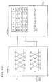
- FIG.10 is a block diagram of the fourth embodiment of the adaptive control system.
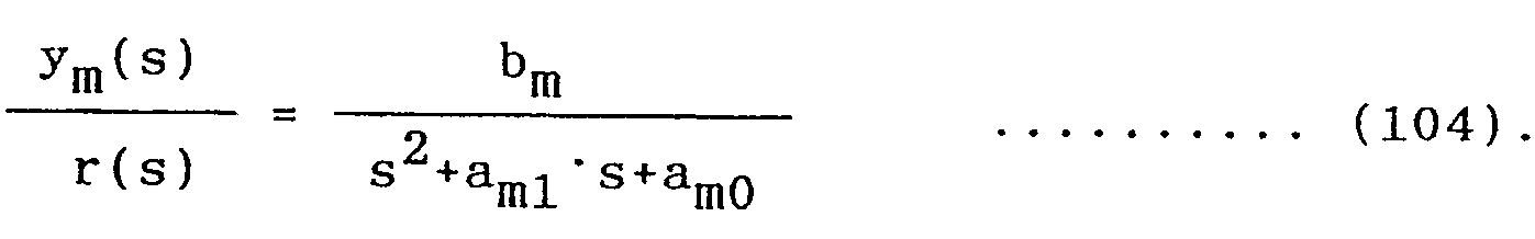
- a reference state output production means 1502 calculation is performed on the basis of equation (104) comprising predetermined reference model coefficients a mi ,a mo and b m with respect to the input of a reference model r(s). Consequently, the reference model output y m (t) of single-input-single-output and the differential value y m (t) thereof are output.
- an error e(t) is calculated from the output y m (t) and the output y(t) detected by the state output detection means 201, and the differential value e(t) of the error is calculated from the differential value y(t) of output y m (t) and the differential value y(t) of the output y(t) on the basis of equation (105).
- the error e(t) and the differential value e(t) of the error are applied to an input calculation means 1504.
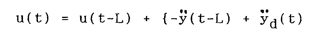
- an input u(t) is calculated by equation (106).
- the equation (107) is corresponds to the equation (56) in the first embodiment.
- equation (56) "K i " is replaced with "(A m,i +K i )" as given by Therefore, the equations introduced in the first embodiment is applicable to the fourth embodiment.
- control input coefficient "best" shown by the equation (106) is selected as given by The equation (109) is identical with the equation (57).
- a control input u(t) is calculated on the basis of the equation (106) by using the control input coefficient "best", the time length "L” and the sum of the reference model coefficient and the error dynamics adjustment matrix "a mi +k i " which satisfy the above-mentioned relations.
- the control input u(t) is applied to a physical plant 200 through a control input production means 205. Consequently, the output of the physical plant having unknown input distribution coefficient meets the output of the reference model.
- the same conversion mentioned above is applicable by applying conversion based on the representation (108). Consequently, the output of the physical plant meets the output of the reference model in the second and third embodiments.
- the adaptive control system also may be constructed by a digital circuit, for example.
- the time length of the product of a sampling periodic time and an integer is selected for the time length "L".
Landscapes
- Engineering & Computer Science (AREA)
- Health & Medical Sciences (AREA)
- Artificial Intelligence (AREA)
- Computer Vision & Pattern Recognition (AREA)
- Evolutionary Computation (AREA)
- Medical Informatics (AREA)
- Software Systems (AREA)
- Physics & Mathematics (AREA)
- General Physics & Mathematics (AREA)
- Automation & Control Theory (AREA)
- Feedback Control In General (AREA)
Abstract
Description
- The present invention relates to an adaptive control system for controlling a physical plant such as a servo motor or a heat pump of which dynamic property can not be estimated and/or extraneous disturbance can not be disregarded.
- In the prior art of the U.S. Patent No. 497257 by Osamu Ito who is one of the inventors of the present application, an example of an adaptive control system is disclosed. In the prior art, a physical plant in which an input distribution matrix "B" is known is described. Moreover, the inventor has disclosed a method for improving a Time Delay Controller (TDC) in the Proceeding of the 31th Japan Joint Automatic Control Conference (page 361 --- 362). According to the method, in the event that an input distribution matrix "B" is unknown, the input distribution matrix "B" is estimated with respect to a single-input-single-output physical plant.
- In the TDC, quick reduction of an error is contemplated. The error is defined by a difference between the output of the physical plant and a "desired trajectory" or the output of a reference model which are defined by a function of time with respect to the physical plant having an unknown property. The "desired trajectory" is defined by an aggregation of data which are given by a function of time and is a target of control in a physical plant. The aggregation of the data is distributed on a trajectory and hence is called the "desired trajectory".
- In order that the output of the physical plant follows a desired trajectory, the value of an input distribution matrix "B" estimated in advance is calculated by dividing the variation of the differential value of the output by the variation of an input thereof. Then, in the TDC, unknown dynamic property other than the input distribution matrix "B" is estimated by using a control input matrix "Best", the input value at a predetermined time length "L" ago and the differential value of the output at the predetermined time length "L" ago. The dispersion of the estimated value of the input distribution matrix "B" is canceled in the control input matrix "Best". Moreover, error characteristic of the TDC is adjusted by using an error dynamics adjustment matrix "Ki". The control input matrix "Best", time length "L" and error dynamic adjustment matrix "K;" are called "design parameters".
- According to the prior art of the U.S. Patent No. 497257, excellent robustness property against unknown dynamic property and/or extraneous disturbance is realized in the event that the variation of an unknown input distribution matrix "B" is relatively small and is slow.
- However, in the TDC of the prior art, some drawbacks exists in view of practical use. Namely, the variation of a small input or a small differential value of an output which is close to zero is used in estimation of the value of an input distribution matrix "B" with respect to an physical plant. Consequently, the estimated value deviates from an actual value, and a control input matrix "Best" having a high accuracy can not be obtained. In order to obtain the control input matrix "Best" having the high accuracy, plural values estimated during a predetermined time length must be calculated by a predetermined process. Namely, the predetermined time length is required for calculation. Therefore, the influence of the unknown dynamic property can not be canceled in an on-line control of the TDC which can response to the practical use. Particularly, the control input matrix "Best" having a high accuracy is not realizable in rapid variation of the input distribution matrix "B". Thus, the physical plant does not follow the desired trajectory, and in a worst case the TDC becomes unstable in the event that the input distribution matrix "B" is unknown.
- On the other hand, in the event that a physical plant which has a large and rapid variation of unknown input distribution matrix "B" is controlled by using a constant control input matrix "Best", and the input distribution matrix "B" varies, a method for determining a control input matrix "Best" for stable operation is not disclosed in the prior art. Furthermore, even if the control input matrix "Best" is determined, a determining method of a time length "L" and an error dynamics adjustment matrix "Ki" is not apparently disclosed to satisfy a "following-property".
- An object of the present invention is to provide an adaptive control system in which a control input matrix "Best" and design parameters can be determined so that the output of a physical plant follows a desired trajectory with stable and excellent following-property in the physical plant of multi-input-multi-output having an unknown input distribution matrix "B".
- In accordance with the present invention, an adaptive control system with respect to the physical plant of q-input-q-output having characteristic of p in number which are represented by an equation

comprises: - trajectory production means for outputting a desired trajectory vector yd(t) of said output vector given by a function of time t and differential value "dyd(t)/dt--dnyd(t)/dtn" of said desired trajectory vector;
- state output detection means for detecting the output vector y(t) of said physical plant and said differential value "dy(t)/dt--d" y(t)/dt"" of said output vector;
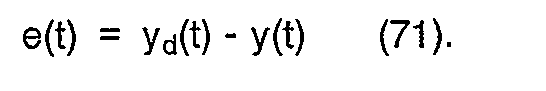
- error value production means for outputting error vector e(t) defined as the equation "e(t)=yd(t)-y(t)" and differential value "de(t)/dt--dn-1e(t)/dtn-1" of said error vector by using
- said desired trajectory vector which is output from said trajectory production means and the differential value of said desired trajectory vector and
- said output vector output from said state output detection means and the differential value of said output vector;
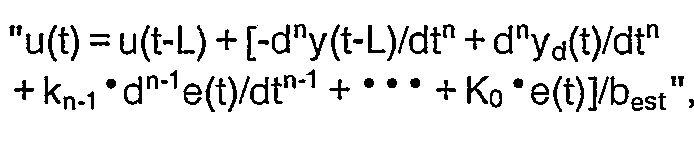
- input calculation means for calculating said input vector u(t) by an equation "u(t) =u(t-L) + Best -1 · [-dny-(t-L)/dtn+dnyd(t)/dtn +Kn-1 · dn-1e(t)/dtn-1 + · + K0·e(t)]" by using
- the differential value of said desired trajectory vector output from said trajectory production means, the differential value "dny(t-L)/dtn" of said output vector which had output from said sate output detection means a time length "L" ago,
- said error vector output from said error value production means,
- the differential value of said error vector and
- preceding input vector "u(t-L)" by the time length "L" ago;
- providing that a qxq-dimension error dynamics adjustment matrix is defined as "Ki(i = n-1--0)", the desired error dynamics is defined as equation "dne(t)/dtn = -Kn-1·dn-1e(t)/dtn-1-···-K0 ·e(t)", a time length being defined as "L" and a control input matrix is defined as "Best";
- means for selecting said control input matrix "Best" in said input calculation means in a manner that entire coefficients with respect to "s" of the characteristic equation which is obtained by equation "det{2Best·Bw -1-I)Ls + 21}" are positive;
- means for selecting said error dynamics adjustment matrix and said time length "L" in a manner that entire conditions given by


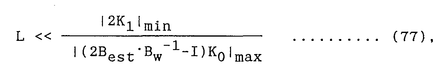
- providing that the minimum absolute value of component of a matrix "2Ki" with the exception of zero component of a matrix "2Ki" is defined as "|2Ki|min", and the frequency range which is required for following-property of said desired trajectory is defined as "ω 0"; and
- control input production means for applying said input vector u(t) which is output from said input calculation means to said physical plant.
- While the novel features of the invention are set forth particularly in the appended claims, the invention, both as to organization and content, will be better understood and appreciated, along with other objects and features thereof, from the following detailed description taken in conjunction with the drawings.
-
- FIG.1 is a perspective view of an example of a physical plant to which the adaptive control system of a first embodiment of the present invention is applied;
- FIG.2 is a block diagram of the adaptive control system of the first embodiment;
- FIG.3 is a diagram of the relation between a time length "L" and a control input coefficient "best";
- FIG.4 is a block diagram of the heat pump system of an example of the physical plant to which a second embodiment of the adaptive control system of the present invention is applied;
- FIG.5 is a block diagram of the second embodiment of the adaptive control system;
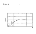
- FIG.6 is a diagram of relation between a desired trajectory and the output of the physical plant;
- FIG.7 is a diagram of the relation between the time length "L" and the control input coefficient "best";
- FIG.8 is a block diagram of a third embodiment of the adaptive control system of the present invention;
- FIGs. 9(a), 9(b), 9(c), 9(d) and 9(e) are block diagrams of relevant parts in FIG.8;
- FIG.10 is a block diagram of a fourth embodiment of the adaptive control system of the present invention.
- It will be recognized that some or all of the Figures are schematic representations for purposes of illustration and do not necessarily depict the actual relative sizes or locations of the elements shown.
- In a physical plant which is represented by a known "state space dynamics equation" given by

- Then, a "desired error dynamics" with respect to the physical plant represented by the equation (1) is represented by equation (2),
- A control input u(t) which satisfies the equation (2) is calculated by equation (3) (see USP 497257 of the prior art),
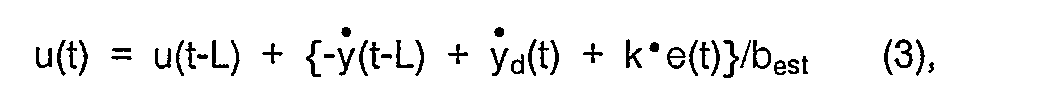
- A control input matrix in the physical plant of multi-input-multi-output is represented by "Best", and a control input matrix in the physical plant of single-input-single-output is represented by "best". Suffix "est" represents estimation value. Then, variable ranges of the equation (1) is given by


- In general, since the time length "L" is very small, the term e-Ls in the equation (5) is simplified by "Pade approximation" as shown in equation (6),

- The equation (6) is substituted for the equation (5), and equation (7) is obtained,


- When the time length "L" is within the ranges shown by relations (11) and (12), "A;" is equal to "Bi(i = 2 --- 0)" within the ranges represented by the relation (4).
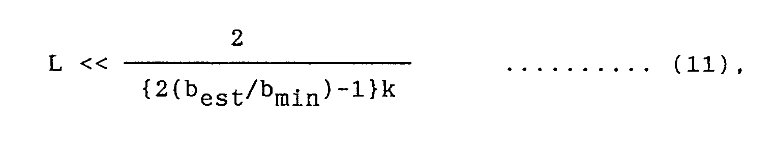
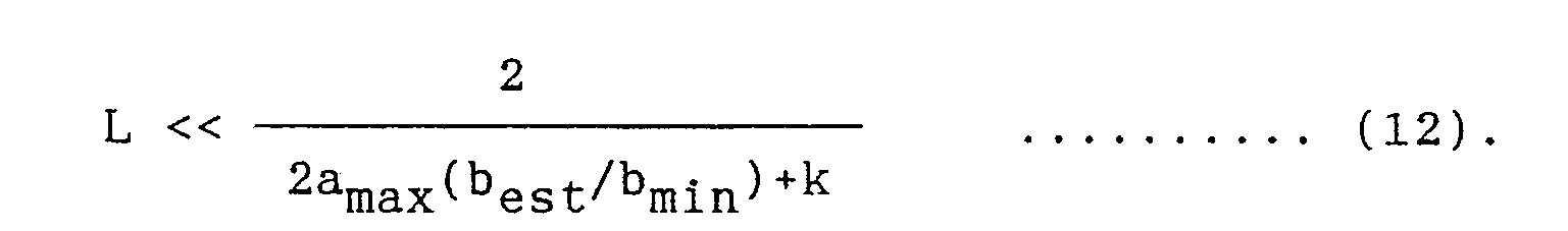
- Namely, when the relations (11) and (12) are satisfied, the polynomial of the denominator of the equation (7) can be substituted for the polynomial Q(s) shown by the equation (9). Then, the transfer function of the equation (7) (right term) is simplified as equation (13) because terms {s + Pk(s)} in numerator and denominator are canceled.

- Referring to the equation (13), within the range shown by the relation (4), condition of stability is to be a negative value in the real part of a pole of the equation (13), and thus the condition of stability is given by
- Moreover, the condition of following-property to the desired trajectory is given by

- Where, m o : a desired frequency range for the following-property. In the physical plant shown by the equation (1), since the desired frequency range M o is equal to the error dynamic adjustment coefficient k(ω o = k) from the desired error dynamics shown by the equation (2), the relations (15), (16) are given by, respectively,
- According to the equations (14) and (18), there is a trade-off relation between stability and following ability in determination of the design parameters of the control input coefficient "best". The stability and the following-property obtained as mentioned above are shown in FIG.3.
- Referring to FIG.3, ordinate is graduated by the time length "L" and abscissa is graduated by the ratio of the control input coefficient "best" to the input distribution coefficient "b".
- Referring to the relation (14), when the control. input coefficient "best" is equal to the control input coefficient "bmax" as shown in the equation (19),

- Subsequently, the adaptive control of a physical plant for a higher order lag system of q-input-q-output is described by using the above-mentioned result hereafter.
- The physical plant is represented by the transfer function given by

- The TDC for calculating the input of the physical plant of multi-input-multi-output corresponding to the equation (3) is given by

- Relations of the higher order lag system corresponding to the relations (11) --- (12) of the first order lag system of single-input-single-output are given by, respectively


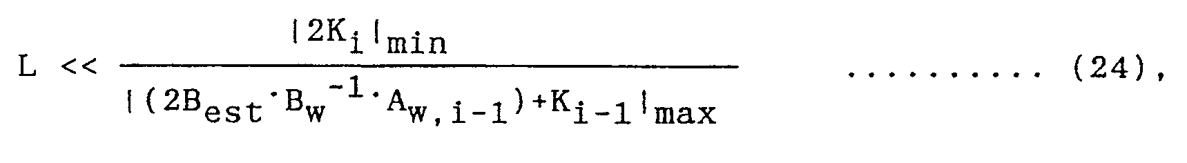

|2Ki|min: minimum absolute value of elements of matrix 2K; except for "0". - When the relations (22) --- (25) are satisfied, the equation corresponding to the equation (13) of the above-mentioned first order lag system of single-input-single-output is given by

- In order to calculate a condition for satisfying stability of the system shown by the equation (26), the following characteristic equation S(s) is used,

- "Routh's stability criterion" is applied to the characteristics equation S(s). In order to satisfy the stability shown by the equation (27), entire coefficients with respect to "s" must be positive. Hence, "necessary conditions" therefor are given by
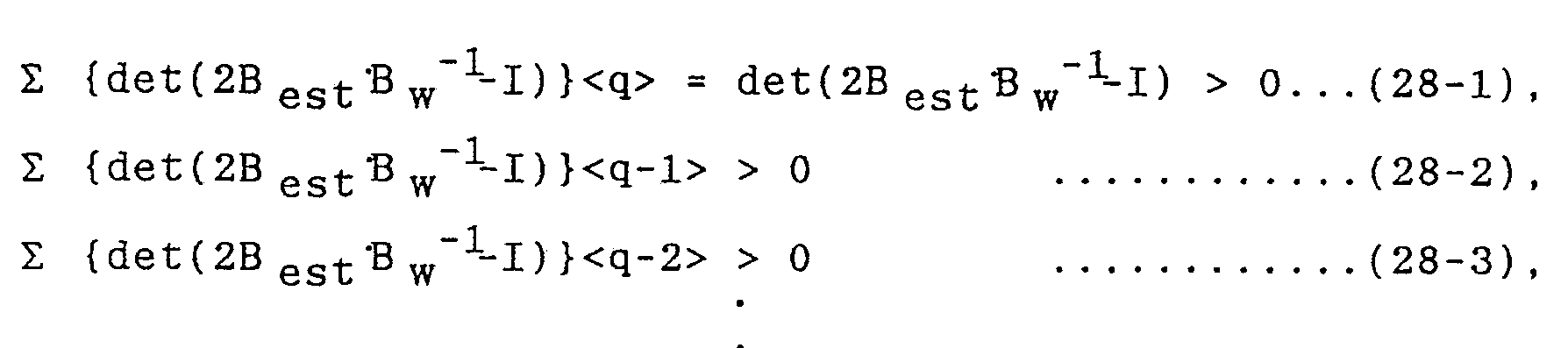

- Moreover, conditions for representing following-property to a desired trajectory corresponding to the equations (15) and (16) of the first order lag system of single-input-single-output are given by


- The relations (28-1) and (30) express "trade-off relation" between stability and following-property in selection of the control input matrix "Best" as a design parameter.
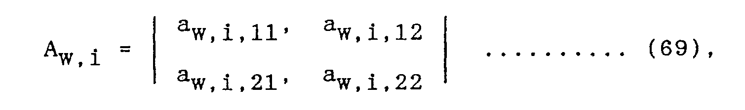
- Hereafter, selection of the control input matrix "Best" is elucidated in detail with respect to the physical plant of two-input-two-output. An input distribution matrix "Bw" and a control input matrix "Best" are defined by equations (31) and (32), respectively.


- Referring to the equations (31) and (32), unknown coefficients "bw" of the input distribution matrix "Bw" are made to fulfill relation (33).

- The equation (27) is a quadratic expression of "s" in the event of two-input-two-output, and both relations (34) and (35) must be satisfied on the basis of the relations (28-1) --- (28-q) as a "necessary and sufficient condition of stability.


- In order to simplify consideration, the sign of (bw,11 --- bW,22) is limited to a positive value as shown in relation (36),

- The equations (31) and (32) are substituted for the relation (35) and are expanded. Then every component of the control input matrix "Best" are bounded as given by
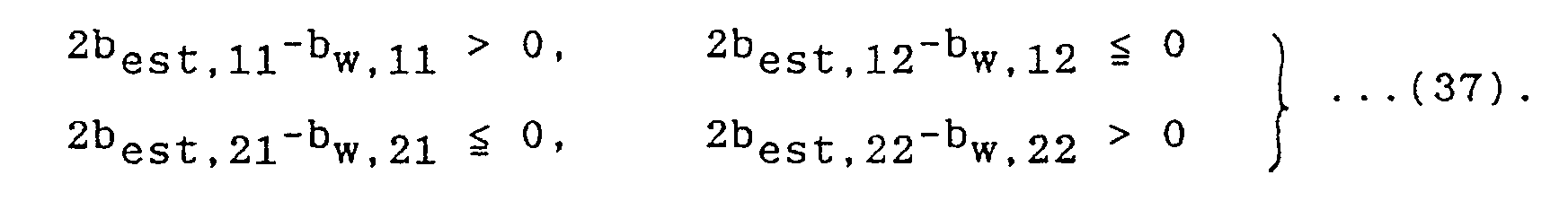
- Consequently, the relation (35) is satisfied. The values of the components of the control input coefficient "best" (best,11, best,12, best,21, best,22) are in the trade-off relation between stability and following-property with each other. Therefore, in order to realize moderate stability, selection shown by relations (38) are recommended.
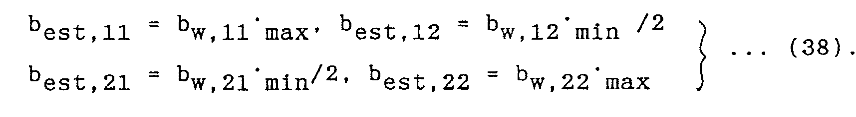
- Moreover, in the event that the relation (33) or the relation (36) is not satisfied, every components of the control input matrix "Best" can be calculated. However, in the event that the sign of the matrix det(Bw) shown by the relation (33) is changed, the control input matrix "Best" can not be determined. Namely, components of the control input matrix "Best" are given by


- The time length "L" of two-input-two-output is calculated by substituting the control input matrix "Best"tor the relations (22) --- (25), (29) and (30), and the time length "L" having the minimum value is selected.
- In the physical plant of three-input-three-output or more, every components of the control input matrix "Best" are selected in a manner that "det(Best)" increases. Then, if the relations (28-1) --- (28-q) are not satisfied, every components of the control input matrix "Best" are changed in a manner that "det(Best)" increases.
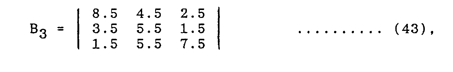
- Stability of the control input matrix with respect to a physical plant of three-input-three-output is calculated by equations (41), (42), (43) and (44).


- In the event that the input distribution matrix "B" varies as shown by the equations (41) --- (43), the following three conditions are applied to the input distribution matrix "B," shown by the equation (41). These three conditions correspond to the equations (28-1) --- (28-q).
- The equation (41) is represented by the equation (45) by using the relation (28-1) --- (28-q).


- The conditions (1), (2) and (3) are satisfied because the values of these equations (46), (47) and (48) are positive values. Consequently, stable operation is realized in the physical plant which has the characteristic of the input distribution matrix "Bi ".
- In a manner similar to that described above, in the event that the conditions (1), (2) and (3) are also satisfied with respect to the equations (42) and (43), the physical plant having the characteristic which varies as shown by the input distribution matrixes "Bi", "B2" and "83" is operated stably by using the input distribution matrix "Best" given by the equation (44).
- FIG.1 is a perspective view of a
servo motor system 106 of a physical plant to which a first embodiment of the adaptive control system in accordance with the present invention is applied. - Referring to FIG.1, a
shaft 101 is rotated by aservo motor 100. Arod 102 is affixed on theshaft 101 and is arranged perpendicularly with respect to the revolution axis of theshaft 101. Aload 105 is supported on therod 102 and is movable along therod 102 as shown by arrow A. Theload 105 is connected to astationary member 107 with intermediates of adamper 103 having viscid material therein and aspring 105. Theload 105 receives a resistant force from thedamper 103 andspring 104 by movement of therod 102 in the direction shown by arrow B and by movement of theload 105 in the direction shown by arrow A. A "viscous resistance" of the damper is represented by "c", and a "spring constant" of thespring 104 is represented by "Ks". Therod 102 comprises a linear motor means, for example, and theload 105 is movable along therod 102 during revolution of theshaft 101, the inertia of themotor system 106 is unknown. - Referring to the above-mentioned physical plant, the revolution angle of the
shaft 101 is represented by "y(t)", and the input torque thereof is represented by "u(t)". - A differential equation for representing the action of the physical plant is given by

- The Laplace transformation of the
physical plant 106 represented by the equation (49) is given by

- The equation (50) represents a transfer function G(s) in the event that an input distribution coefficient "bw" is unknown and is varied.
- The variable range of unknown characteristic "aW,i" and the input distribution coefficient "bw" are given by

- The block diagram of the adaptive control system of the first embodiment is shown in FIG.2. Referring to FIG.2, a
physical plant 200 corresponds to themotor system 106 shown in FIG.1. The revolution angle, angular velocity and angular acceleration of thephysical plant 200 are detected by anoutput sensor 201 comprising an encoder, a tachometer, an acceleration sensor and a processing circuit therefor. - An arbitrary desired trajectory yd(t) of the angular acceleration of the function of time, differential values yd(t) and yd(t) of the desired trajectory yd(t) are output from a trajectory production means 202.
- The desired trajectory yd(t) and the differential value yd(t) of the desired trajectory yd(t) are applied to an error value production means 203. In the error value production means 203, an output y(t) output from the state output detection means 201 and the differential value y(t) of the output y(t) are also applied to the error value production means 203, and calculation is performed on the basis of the equation (54).

- The error e(t), the differential value e(t) and the second order differential value yd(t) of the output of the trajectory production means 202 are applied to an input calculation means 204. Moreover, an angle acceleration y(t-L) of the output of the state output detection means 201 which has detected a predetermined time length "L" ago is also inputted to the input calculation means 204. Then, calculation is performed on the basis of equation (55) by using an input u(t-L) which has inputted the time length "L" ago.

- Referring to the equation (55), "k," and "ko" represent "error dynamics adjustment coefficients", and "best" represents a "control input coefficient" which is used to calculate the control input u(t).
- A "desired error dynamics" which is represented by the following equation (56) is satisfied by these equations (50), (54) and (55):

- Referring to the equation (55), the control input coefficient "best" is selected to satisfy the relation (14) as following equation (57):


- Then, in the input calculation means 204, calculation is performed on the basis of the control input coefficient "best" and the time length "L". Consequently, the resultant control input u(t) is converted into an input torque U(t) by a control input production means 205 which comprises an actuator or a driving circuit therefor, and is applied to the
physical plant 200. Thus, the output y(t) of thephysical plant 200 which is produced by the applied input torque U(t) is controlled to confirm the desired trajectory. - According to the first embodiment, in order to make the output of the physical plant to follow the desired trajectory, the control input therefor is calculated by the input calculation means 204 on the basis of the control input coefficient "best" and the time length "L", and hence the physical plant having unknown input distribution coefficient is made to follow the predetermined desired trajectory.
- FIG.3 is a graph representing relation between the time length "L" and the ratio

- A second embodiment of the adaptive control system in accordance with the present invention is to be applied to the physical plant of two-input-two-output having unknown input distribution matrix.
- In the second embodiment, a heat pump system is taken as an example of the physical plant.
- FIG.4 is a block diagram of the
heat pump system 506, and FIG.5 is a block diagram of the adaptive control system for controlling theheat control system 506. - Referring to FIG.4, a
compressor 501, acondenser 503, anexpansion valve 505 and anevaporator 500 are coupled in loop-shape by fourpipe lines 507, and refrigerant is circulated through these pipe lines 507. Awater line 508A is arranged adjacent to theevaporator 500, and the refrigerant is given heat from the water flowing thewater line 508A. Then the refrigerant is compressed by thecompressor 501 which is driven by aninverter 502. The compressed refrigerant is flowed in thecondenser 503. Anotherwater line 508B is arranged adjacent to thecondenser 503, and the flow rate of the water is controlled by awater pump 504. In thecondenser 503, heat of the refrigerant is given to the water flowing thewater line 508B. Then the refrigerant is returned to theevaporator 500 through anexpansion valve 505. - FIG.5 is a block diagram of the adaptive control system of the second embodiment. A
physical plant 600 in FIG.5 corresponds to theheat pump system 506 of FIG.4. A state output detection means 601 comprises atemperature sensor 509 for detecting temperature of the water at an outlet, atemperature sensor 510 for detecting temperature of water at an inlet thereof and aflow rate sensor 511. - First, a temperature To(` C) which is a first output y1 is detected by the
temperature sensor 509. Second, a temperature Tin(°C) is detected by thetemperature sensor 510. Then, a temperature difference Tsub( C) is calculated by subtracting the temperature Tin from the temperature To. Then, a second output y2 of a calorie q(kcal/h) is calculated on the basis of the temperature difference Tsub( C) and a flow rate G (kg/h) which is detected by aflow rate sensor 511 as shown in equation (64).
water pump 504 and a voltage applied to theinverter 502, dynamic characteristic at various operational point of p(w = 1---p) in number is given by


- Subsequently, the desired trajectory vector "yd(t) = [y1d(t), y2d(t)]T" of temperature and calorie which are functions of time and a differential value of the desired trajectory vector are output from a trajectory production means 602.
- Then, in an error value production means 603, calculation of equation (71) is performed, and an error vector e(t) and a differential value e(t) of the error vector are output therefrom.
- Moreover, in an output calculation means 604, calculation of equation (72) is performed, and a control input u(t) is output.

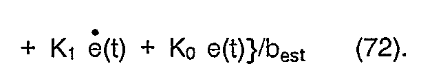
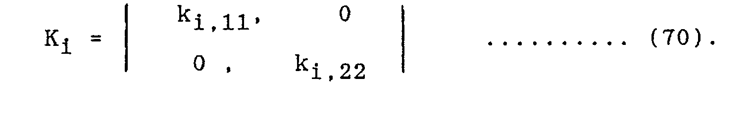
- In the equation (72), "L" represents a predetermined time length, "u(t-L)" represents the input vector which had applied to the physical plant the time length L ago, and "y(t-L)" represents the output vector which had detected by the state output detection means 601 the time length L ago, "Ki " and "Ko" are error dynamics adjustment matrixes and "Best" represents a control input matrix which is used to calculate a control input vector u(t).
- Where, the control input matrix "Best" is the value given by

- The relations (78) and (79) relate to the following-property to the desired trajectory.


- Then, the control input vector u(t) which is output from the input calculation means 604 is converted into an input vector "U(t)" by a control input production means 605 which comprises an actuator and a driving circuit therefor and is applied to the
physical plant 600. Hence, the output "y(t)" of thephysical plant 600 is controlled to follow the desired trajectory in compliance with the input vector "U(t)". - According to the second embodiment, the output of the physical plant of two-input-two-output is controlled to follow the desired trajectory by using the control input matrix "Best" and the time length "L". Thus, the output of the physical plant having unknown input distribution matrix "B" is made to follow the desired trajectory.
- Moreover, the physical plant having multi-input-multi-output can be controlled by using design parameters which satisfy the relations (28-1 )--(28-q) with respect to the control input matrix "Best", and by using the relations (22)--(25), (29) and (30) with respect to the time length L, and a similar effect is realizable. Referring to the relations (74)--(77), the time length "L" is selected in advance, and then the error dynamic adjustment matrix "Ki" can be determined so as to satisfy the time length "L" selected in advance. Hence a similar result is realizable.
- In the third embodiment, a control input coefficient "best" is changed during operation of the adaptive control system so as to approach an actual input distribution coefficient "b". Consequently, the following-property of the output of a physical plant is further improved.
- In the event that a control input coefficient "best" is significantly different from the input distribution coefficient "b" of the physical plant, and a time length "L" is relatively longer, the following-property with respect to a desired trajectory is deteriorated as shown in FIG.6. Referring to FIG.6, abscissa is graduated by the passage of time "t", and ordinate is graduated by the output of a physical plant and the desired trajectory thereof. The curve "y" representing the output of the physical plant is spaced from the curve "yd" representing the desired trajectory.
- In order to improve the following-property, the time length "L" is set to the value as mentioned in the second embodiment (relations (74)---(79)). Then, the initial value of a control input coefficient "best" is set to the control input coefficient "bmax" so as to maintain stability with respect to variation of an input distribution coefficient "b". In the event that the following-property is not satisfied by the above-mentioned operation, the control input coefficient "best" is varied in a manner that the following-property is improved. The above-mentioned operation is described in detail below.
- (I) The error "e" and a differential value "e" of the error output from the error value production means 1303 in FIG.8 are compared with a predetermined value of an error "f;". Consequently, in the event that at least one of the conditions shown by relations (80), (81) and (82) are satisfied, it is determined that the following-property is bad. The comparison is performed during a predetermined set-time length tlim or more.
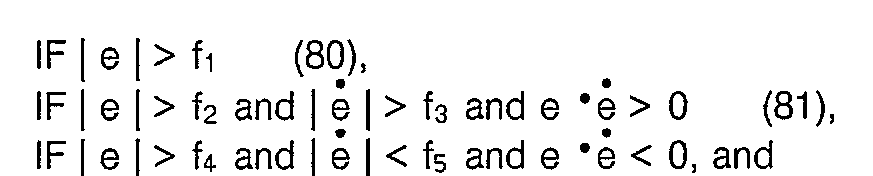
- In first order lag system, determination is performed by relation (85) as replacement for the relation (82).

- When a periodic time of control is equal to the time length Tiim, the following-property is determined every periodic times.
- The error is a time-variant value. Therefore, in the event that the conditions shown by the relations (80), (81) and (82) are not satisfied owing to the variation of the error, a time length Tiim for satisfying the condition of the relation (80), for example, is detected during the set-time length tlim. Then, the ratio (rlim) of the time length T,;m to the set-time length tlim is calculated as shown by relation (83), and the ratio (rlim) can be used to determine the following-property.

- An average values of the error and the differential value of the error are usable as replacements for the error and the differential value of the error, and an example thereof is given by


- In a similar manner, as described with respect to the relations (80), (81) and (82), when the periodic time of control is equal to the set-time length tlim, stability is determined every the periodic time. When the set-time length tlim is relatively longer, determination of the stability is performed by continuous several times of satisfaction of the conditions given by the relation (86) or (87).
- Design parameters can be changed in order to improve the following-property and stability as described below.
- A control input coefficient "best" is reduced at a predetermined rate by multiplying a control input coefficient "best" by a predetermined constant Cd which is smaller than "1.0" as shown by equation (88).


- Moreover, an average absolute value of an error (|e|ave) during the setting time tlim is usable as replacement for the absolute value of an error (|e|).
- The control input coefficient "best" is maintained as shown by equation (91).

- Moreover, the control input coefficient "best" in the equation (90) is made to the control input coefficient "bmax" as shown by equation (92).

- Referring to the relations (88) and (89), the control input coefficient "best" is progressively reduced apart from an initial value of the control input coefficient ("bmax", for example) by the calculation of the relations (88) and (89). Consequently, the control input coefficient "best" approaches an optimum control input coefficient "bi ". Consequently, the error decreases, and thus the following-property is improved.
- The above-mentioned method is applicable to a physical plant of which the control input coefficient "b" is temporarily varied. Such case is shown, in FIG.1, in the example that the
load 105 is moved along therod 102 to a predetermined position, and after then theload 105 is held at the position. - In the event that the control input coefficient "b" is quickly varied, the variation method shown by equations (90) and (92) are preferable. Referring to the equations (90) and (92), the control input coefficient "best" is varied when the error is large, and in this case, the control input coefficient "best" is made to the control input coefficient "bmax".
- (III) In the event that the stability is bad.
- The control input coefficient "best" is made to increase at a constant rate by multiplying the input coefficient "best" by a predetermined constant Cu which is larger than 1.0 as shown by the relation (93).

- Alternatively, the control input coefficient "best" can be made to the control input coefficient "bmax" as shown by relation (94).

- In the event that both the following-property and stability are bad, the stability is improved with priority.
- Calculations by the relations (80) --- (87) can be performed by fuzzy inference calculation. In the fuzzy inference calculation, the situation part comprise variables for determining following-property, and the action part comprises variables for varying design parameters.
- An example of the fuzzy inference representation is given by

- When an error "e" and the differential value "e" of the error "e" are inputted, the following result is obtained by the fuzzy inference representation (95):

- The fuzzy inference calculation comprises a plurality of the fuzzy inference representations. Consequently, the final result of the fuzzy inference calculation is given by
- An example of the adaptive control system using the fuzzy inference calculation will be described hereafter in reference with FIG.9(d).
- In a physical plant which is influenced by a dead-time, low-order-approximation, the optimum design parameter can be obtained by an experimental method. According to the experimental method, the control input coefficient "best" of the TDC as shown by the equation (3), error dynamics adjustment matrix "ki" and time length "L" are automatically varied.
- FIG.7 is a graph of the relation between the time length "L" and the ratio of the control input coefficient "best" to the input distribution coefficient "b" for illustrating the areas of stability and following-property of an actual physical plant of single-input-single-output. Referring to FIG.7, ordinate is graduated by the time length "L", and abscissa is graduated by the ratio of the control input coefficient "best" to the control input distribution coefficient "b". An unstable area Q is produced by a parasitic mode such as the dead-time or the higher order dynamic characteristic.
- On the other hand, in order to improve the following-property, the stable-and-good-following-property area is liable to be narrowed. Furthermore, there is occasion where the design parameters lack the proper stable-and-good-following-property area.
- In the event that the adjustment of the design parameters is impossible, a response speed which gives influence to the following-property must be reduced by decreasing the error dynamics adjustment matrix "Ki". Consequently, the control input coefficient "best" is increased. In the above-mentioned case, since the following-property is deteriorated by increase of the control input coefficient "best", a slight reduction of the control input coefficient "best" is recommendable to improve the following-property. However, in the event that the ratio of the control input coefficient "best" to the control input distribution coefficient "b" is lesser than 0.5 (best/b < 0.5), the adaptive control system is oscillated.
- If the time length "L" is reduced, the following-property is improved. However, excessive reduction of the time length "L" results in oscillation of the adaptive control system in the event that the influence of the higher order dynamic characteristic or the dead-time can not be disregarded.
- Moreover, excessive increase of the error dynamics adjustment coefficient ki results in oscillation of the adaptive control system. Therefore, there is no compatibility in change of the design parameters. Then, the initial value of the control input coefficient "best"is set to the control input coefficient "bmax". In the event that the parasitic mode influences to the following-property in such initial value, one of the following changes is performed:
- The control input coefficient "best" is increased.
- The dynamics adjustment coefficient "ki" is decreased.
- The time length "L" is increased. Consequently, the stability is improved by the above-mentioned change of the design parameters.
- According to the third embodiment, the error or the differential value of the error of the actual input distribution coefficient "b" are determined with respect to the physical plant of single-input-single-output by change of the control input coefficient "best" on the basis of the error, the differential value of the error or the differential value of the input. Then, the control input coefficient "best" is changed in real time, and thereby the output of the physical plant is made to follow the desired trajectory.
- FIG.8 is a block diagram of the third embodiment of the adaptive control system. Referring to FIG.8, the
physical plant 200, the state output detection means 201, the trajectory production means 202, the error value production means 203 and the control production means 205 are identical with those of the first embodiment. - In a first output judgment means 1306, following-property is determined by using the error e(t), in the event that the absolute value of the error is larger than a predetermined value fi as shown by relation (98).

- Moreover, in a second output judgment means 1307, stability is determined by using the second order differential value of the error as shown by relation (99).

- When bad following-property is determined by satisfying the relation (98), calculation given by equation (100) is performed by using the absolute value of the error within the time tlim in the first parameter change means 1308.

- When the relation (98) is not satisfied, good following-property is determined by the first output judgment means 1306. Consequently, as shown by equation (101), the control input coefficient "best" is not changed and is held to the value at the last time.
- When the relation (99) is satisfied and bad stability is determined, in a second parameter change means 1309, the control input coefficient "best" is increased as given by relation (102).

- When the relation (99) is not satisfied, good stability is determined by the second output judgment means 1307, the control input coefficient "best" is not output by the second parameter change means 1309. Then the control input coefficient "best" which is output from the second parameter change means 1309 has priority to the control input coefficient "best" output from the first parameter change means 1308. The priority is determined by the parameter determination means 1310. Then, in the event that the control input coefficient "best" is output from the second parameter change means 1309, the control input coefficient "best" is employed by the parameter determination means 1310. On the other hand, in the event that the control input coefficient "best" is not output from the second parameter change means 1309, the control input coefficient "best" output from the first parameter change means 1308 is employed by the parameter determination means 1310.
- Subsequently, a control input u(t) is calculated by equation (103) in an input calculation means 1304 by using the control input coefficient "best" output from the parameter determination means 1310.

- The time length "L" is set to a value which satisfies the relations (58) --- (63) in a similar manner of the first embodiment. Moreover, the initial value of the control input coefficient "best" is set to the control input coefficient "bmax" as given by the equation (57). The control input u(t) is applied to the
physical plant 200 through the control input production means 205. - FIGs. 9(a), 9(b), 9(c), 9(d) and 9(e) are block diagrams of relevant parts of the third embodiment for partially changing the configuration in FIG.8.
- Referring to FIG.9(a), a first and a second output judgment means 1406(a) and 1407(a) correspond to the first and second output judgment means 1306 and 1307 in FIG.8, respectively. Moreover, a first and a second parameter change means 1408(a) and 1409(a) correspond to the first and second parameter change means 1308 and 1309 in FIG.8, respectively. In the configuration, in the event that bad following-property is determined, the control input coefficient "best" or the time length "L" is decreased, or the error dynamics adjustment coefficient "k" is increased. On the other hand, in the event that bad stability is determined, the control input coefficient "best" or the time length "L" is increased, or the error dynamics adjustment coefficient "k" is decreased.
- In the example shown by FIG.9(b), the first output judgment means 1406(b) is comprised as replacement for the first output judgment means 1306, thereby calculation based on the relation (83) is performed. By the calculation, the ratio of a predetermined setting time tlim to a time length Turn in which the error value "e" exceeds a predetermined error value "fi" during the setting time tnm is obtained. When the ratio is larger than a predetermined value rnm, bad following-property is determined. Then, stable control is realizable by increasing the setting-time tlim, and hence stable control is realizable.
- In a physical plant in which an input distribution coefficient is quickly varied, a first parameter change means 1408(c) shown in FIG.9(c) is used as replacement for the first parameter change means 1308 in FIG.8. In the first parameter change means 1408(c), calculation based on the equation (90) or equation (92) is performed in accordance with the output of the first output judgment means 1306 which is inputted to the first parameter change means 1408(c). Namely, in the event that the output of the first judgment means 1306 is "Yes" (the error value is larger than a predetermined value), the calculation of the equation (90) is performed, and the control input coefficient "best" is varied in accordance with the error value. On the other hand, in the event that the output of the first output judgment means 1306 is "No" (the error value is smaller than the predetermined value), the control input coefficient "bmax" which is a maximum control input coefficient is employed.
- FIG.9(d) is a block diagram of an example using fuzzy inference calculation in a first output judgment means 1406(d) and a second parameter change means 1408(d). In the fuzzy inference calculation, five fuzzy variables of NB (negative big), NS (negative small), ZO (zero), PS (positive small), and PB (positive big) are set in the first output judgment means 1406(d). Data of an error "e" and the differential value "e" of the error "e" are memorized with a predetermined normalizing coefficient. The real values "q;" are selected in accordance with the fuzzy variables of the error "e" and the differential value "e" of the error "e" as shown in a table of the second parameter change means 1408(d). The normalizing coefficient and the real value "qi" are selected in a manner that the following property is improved.
- Moreover, every design parameters are experimentally changed to obtain optimum values for the physical plant having inaccurate transfer function or a parasitic mode. In the above-mentioned case, as shown in FIG.9(e), a first and second output judgment means 1406(e) and 1407(e) are used as replacements for the first and second output judgment means 1306 and 1307, respectively. Moreover, a first and a second parameter change means 1408(e) and 1409(e) are used as replacements for the first and second parameter change means 1308 and 1309, respectively. In operation, the design parameters of the control input coefficient "best", time length "L" and the error dynamics adjustment matrix "k" are changed on the basis of the result of judgment by the first and second output judgment means 1406(e) and 1407(e) in order to determine optimum design parameters. In the above-mentioned case, the initial values of the control input coefficient "best" and the time length "L" can be selected from arbitrary values.
- In the first, second and third embodiments mentioned above, the description is related to the adaptive control system for controlling a physical plant to a predetermined desired trajectory. In the fourth embodiment, the physical plant is controlled to the output which is instructed by a reference model.
- FIG.10 is a block diagram of the fourth embodiment of the adaptive control system. Referring to FIG.10, in a reference state output production means 1502, calculation is performed on the basis of equation (104) comprising predetermined reference model coefficients ami,amo and bm with respect to the input of a reference model r(s). Consequently, the reference model output ym(t) of single-input-single-output and the differential value ym(t) thereof are output.
-
- In the error value production means 203, an error e(t) is calculated from the output ym(t) and the output y(t) detected by the state output detection means 201, and the differential value e(t) of the error is calculated from the differential value y(t) of output ym(t) and the differential value y(t) of the output y(t) on the basis of equation (105).

- In the input calculation means 1504, an input u(t) is calculated by equation (106).


- Consequently, a desired error dynamics is calculated on the basis of equations (104), (105) and (106), and is represented by equation (107).

- In the fourth embodiment, the equation (107) is corresponds to the equation (56) in the first embodiment. In the equation (56), "Ki" is replaced with "(Am,i+Ki)" as given by

- In a similar manner mentioned above, the control input coefficient "best" shown by the equation (106) is selected as given by

- Moreover, in determination of the time length "L", "ki" in the equations (58), (59), (60) and (61) is replaced with "(am,i+k¡)", and consequently, equations (110), (111), (112), (113), (114) and (115) are obtained.


- Then, the time length "L" is determined which satisfies entire conditions given by these relations (110 115).
- In the input calculation means 1504, a control input u(t) is calculated on the basis of the equation (106) by using the control input coefficient "best", the time length "L" and the sum of the reference model coefficient and the error dynamics adjustment matrix "ami+ki" which satisfy the above-mentioned relations. The control input u(t) is applied to a
physical plant 200 through a control input production means 205. Consequently, the output of the physical plant having unknown input distribution coefficient meets the output of the reference model. - Moreover, in the second embodiment and the third embodiment, the same conversion mentioned above is applicable by applying conversion based on the representation (108). Consequently, the output of the physical plant meets the output of the reference model in the second and third embodiments.
- The adaptive control system also may be constructed by a digital circuit, for example. In such case, the time length of the product of a sampling periodic time and an integer is selected for the time length "L".
- Although the present invention has been described in terms of the presently preferred embodiments, it is to be understood that such disclosure is not to be interpreted as limiting. Various alterations and modifications will no doubt become apparent to those skilled in the art after having read the above disclosure. Accordingly, it is intended that the appended claims be interpreted as covering all alterations and modifications as fall within the true spirit and scope of the invention.
Claims (11)
comprising:
comprising:
comprising:
Applications Claiming Priority (4)
| Application Number | Priority Date | Filing Date | Title |
|---|---|---|---|
| JP7605890 | 1990-03-26 | ||
| JP76058/90 | 1990-03-26 | ||
| JP29573190 | 1990-10-31 | ||
| JP295731/90 | 1990-10-31 |
Publications (2)
| Publication Number | Publication Date |
|---|---|
| EP0449169A2 true EP0449169A2 (en) | 1991-10-02 |
| EP0449169A3 EP0449169A3 (en) | 1992-03-25 |
Family
ID=26417221
Family Applications (1)
| Application Number | Title | Priority Date | Filing Date |
|---|---|---|---|
| EP19910104658 Withdrawn EP0449169A3 (en) | 1990-03-26 | 1991-03-25 | Adaptive control system |
Country Status (2)
| Country | Link |
|---|---|
| US (1) | US5355065A (en) |
| EP (1) | EP0449169A3 (en) |
Cited By (1)
| Publication number | Priority date | Publication date | Assignee | Title |
|---|---|---|---|---|
| EP1251026A3 (en) * | 1998-04-28 | 2003-05-07 | Toyota Jidosha Kabushiki Kaisha | Control system for reduction of vibrations in vehicle having continuously variable transmission |
Families Citing this family (5)
| Publication number | Priority date | Publication date | Assignee | Title |
|---|---|---|---|---|
| DE4317538A1 (en) * | 1993-05-26 | 1994-12-01 | Siemens Ag | Control device |
| JP3070341B2 (en) * | 1993-07-20 | 2000-07-31 | 株式会社日立製作所 | Inverter frequency control method and device |
| US5796922A (en) * | 1996-03-29 | 1998-08-18 | Weber State University | Trainable, state-sampled, network controller |
| US6163730A (en) * | 1997-08-11 | 2000-12-19 | Motorola, Inc. | Method and control system for changing the state of a plant |
| JP2001255903A (en) * | 2000-03-14 | 2001-09-21 | Toshiba Corp | Process control system |
Family Cites Families (1)
| Publication number | Priority date | Publication date | Assignee | Title |
|---|---|---|---|---|
| EP0389281A3 (en) * | 1989-03-23 | 1991-09-25 | Matsushita Electric Industrial Co., Ltd. | Adaptive control system |
-
1991
- 1991-03-25 EP EP19910104658 patent/EP0449169A3/en not_active Withdrawn
-
1993
- 1993-05-11 US US08/060,039 patent/US5355065A/en not_active Expired - Fee Related
Cited By (1)
| Publication number | Priority date | Publication date | Assignee | Title |
|---|---|---|---|---|
| EP1251026A3 (en) * | 1998-04-28 | 2003-05-07 | Toyota Jidosha Kabushiki Kaisha | Control system for reduction of vibrations in vehicle having continuously variable transmission |
Also Published As
| Publication number | Publication date |
|---|---|
| EP0449169A3 (en) | 1992-03-25 |
| US5355065A (en) | 1994-10-11 |
Similar Documents
| Publication | Publication Date | Title |
|---|---|---|
| US6037736A (en) | Apparatus for determination of control constant | |
| Suleiman et al. | Methods of chattering reduction in sliding mode control: A case study of ball and plate system | |
| EP0494500A1 (en) | Sliding mode control system | |
| US4744511A (en) | Air conditioner for automobiles | |
| US5276387A (en) | Sliding mode control system | |
| EP0449169A2 (en) | Adaptive control system | |
| Hwang et al. | Comparison on fuzzy logic and PID controls for a DC motor position controller | |
| Salem et al. | Enhancing cruise performance through pid controller tuned with particle swarm optimization technique | |
| Dashti et al. | Neural—Adaptive control based on backstepping and feedback linearization for electro hydraulic servo system | |
| Pillai et al. | Intelligent adaptive controller for DC servo motor position control in LabVIEW | |
| Sinthipsomboon et al. | A hybrid of fuzzy and fuzzy self-tuning PID controller for servo electro-hydraulic system | |
| CN112542974B (en) | Motor control system | |
| Kumbasar et al. | Self-tuning interval type-2 fuzzy PID controllers based on online rule weighting | |
| EP1164448A2 (en) | Control apparatus | |
| McDowell et al. | Online neural control applied to a bank-to-turn missile autopilot | |
| JP2502839B2 (en) | Adaptive controller | |
| JP4036520B2 (en) | Simple adaptive controller | |
| Das et al. | Fuzzy Fractional Order PID Controller Design for Single Link Robotic Arm Manipulator | |
| JPH07219601A (en) | Adjuster | |
| Khinchi et al. | Control of electronic throttle valve using model predictive control | |
| Chen et al. | Application of feedback linearization to tracking and almost disturbance decoupling control of the AMIRA ball and beam system | |
| Leiviskä et al. | Design of adaptive fuzzy controllers | |
| JPH0577656A (en) | Constant-speed traveling control device for vehicle | |
| JP2837691B2 (en) | Exercise machine control device | |
| JPH08194542A (en) | Overshoot-less auto tuning method |
Legal Events
| Date | Code | Title | Description |
|---|---|---|---|
| PUAI | Public reference made under article 153(3) epc to a published international application that has entered the european phase |
Free format text: ORIGINAL CODE: 0009012 |
|
| 17P | Request for examination filed |
Effective date: 19910325 |
|
| AK | Designated contracting states |
Kind code of ref document: A2 Designated state(s): DE FR GB |
|
| PUAL | Search report despatched |
Free format text: ORIGINAL CODE: 0009013 |
|
| AK | Designated contracting states |
Kind code of ref document: A3 Designated state(s): DE FR GB |
|
| 17Q | First examination report despatched |
Effective date: 19940527 |
|
| STAA | Information on the status of an ep patent application or granted ep patent |
Free format text: STATUS: THE APPLICATION IS DEEMED TO BE WITHDRAWN |
|
| 18D | Application deemed to be withdrawn |
Effective date: 19941007 |