EP0447328A2 - Scalar data processing method and apparatus - Google Patents
Scalar data processing method and apparatus Download PDFInfo
- Publication number
- EP0447328A2 EP0447328A2 EP91400712A EP91400712A EP0447328A2 EP 0447328 A2 EP0447328 A2 EP 0447328A2 EP 91400712 A EP91400712 A EP 91400712A EP 91400712 A EP91400712 A EP 91400712A EP 0447328 A2 EP0447328 A2 EP 0447328A2
- Authority
- EP
- European Patent Office
- Prior art keywords
- scalar data
- dimensional
- function
- edge lines
- data
- Prior art date
- Legal status (The legal status is an assumption and is not a legal conclusion. Google has not performed a legal analysis and makes no representation as to the accuracy of the status listed.)
- Granted
Links
Images


Classifications
-
- H—ELECTRICITY
- H04—ELECTRIC COMMUNICATION TECHNIQUE
- H04N—PICTORIAL COMMUNICATION, e.g. TELEVISION
- H04N19/00—Methods or arrangements for coding, decoding, compressing or decompressing digital video signals
-
- H—ELECTRICITY
- H04—ELECTRIC COMMUNICATION TECHNIQUE
- H04N—PICTORIAL COMMUNICATION, e.g. TELEVISION
- H04N19/00—Methods or arrangements for coding, decoding, compressing or decompressing digital video signals
- H04N19/20—Methods or arrangements for coding, decoding, compressing or decompressing digital video signals using video object coding
Definitions
- the present invention relates to a scalar data processing apparatus and a method for compressing two-dimensional scalar data and for reconstructing the compressed two-dimensional scalar data.
- two-dimensional scalar data ⁇ (x,y) such as luminance data of a picture on a two-dimensional surface or concave-convex data of a relief formed on a wall surface
- L(x,y) is a scalar potential such as the luminance
- R ⁇ K is a vector potential having a direction expressed by a unit vector K in the direction of the Z axis.
- the lamellar component is the first item, i.e., grad L, in the above expression (1)
- the vortex component is the second item, i.e., rot (R ⁇ K), in the above expression (1).
- the present invention was conceived from the above proposal with respect to the chrominance component.
- the present invention has an object to enable a reduction in the amount of data in the transmission or storing of two-dimensional scalar data by compressing two-dimensional data by the boundary value on the edge lines and by applying an interpolation by the use of the compressed data.
- An edge line of the scalar data is determined as a place where the divergence and rotation of the vector are greatly changed.
- the divergence of the vector in the expression (2) is
- the rotation of the vector V in the expression (2) is
- the edge line of the scalar data ⁇ can be determined by detecting only the divergence of the gradient ⁇ , i.e., the Laplacian ⁇ ⁇ , which exceeds the predetermined threshold value. Since the rotation of the vector V is always zero, it is not necessary to consider the rotation of the vector V.
- the Laplacian ⁇ ⁇ the absolute value of which exceeds the predetermined threshold value can be detected by detecting the value ⁇ and its gradient on the edge line. Once the value ⁇ and its gradient on the edge line are given, the values ⁇ at the other points can be estimated by interpolation because the values ⁇ at the other points are changed loosely.
- a scalar data processing method and apparatus for compressing two-dimensional scalar data defined on a two-dimensional surface having a horizontal direction and a vertical direction and for reconstructing the two-dimensional scalar data based on the compressed data.
- the method comprises the step of detecting edge lines of the two-dimensional scalar data. The edge lines are detected in such a way that the change of the value of the two-dimensional scalar data between adjacent points on the two-dimensional surface is larger than a predetermined threshold value.
- the method further comprises the steps of cutting a domain along a horizontal line intersecting with the edge lines and between the edge lines; determining a function as an approximation of a Laplacian of the two-dimensional scalar data at each point in the cut domain; compressing the two-dimensional scalar data by replacing the two-dimensional scalar data at every point with scalar data at the edge lines, scalar data for providing gradients of the two-dimensional scalar data on the edge lines, and the function determined in the above step; and reconstructing the two-dimensional scalar data by interpolating the two-dimensional scalar data based on the scalar data at the edge lines, scalar data for providing gradients of the two-dimensional scalar data on the edge lines, and the function obtained in the above compressing step.
- the scalar data processing apparatus comprises an edge line detecting unit for detecting edge lines of the two-dimensional scalar data; a domain cutting unit for cutting a domain on a horizontal line intersecting with the edge lines and between the edge lines; a function determining unit for determining a function as an approximation of a Laplacian of the two-dimensional scalar data at each point in the cut domain; a compressing unit for compressing the two-dimensional scalar data by replacing the two-dimensional scalar data at every point with scalar data at the edge lines, scalar data for providing gradients of the two-dimensional scalar data on the edge lines, and the function determined in the above compressing unit ; and a reconstructing unit for reconstructing the two-dimensional scalar data by interpolating the two-dimensional scalar data based on the scalar data at the edge lines, scalar data for providing gradients of the two-dimensional scalar data on the edge lines, and the
- Figure 1 is a flowchart showing the principle operation of the scalar data processing according to an embodiment of the present invention.
- the right hand side of the flowchart represents a picture on a display 10.
- reference 10 represents a display in which "i" represents an x coordinate in the horizontal direction and "j" represents a y coordinate in the longitudinal direction, 11-1 and 11-2 represent the edge lines, 12 represents a domain cut by the edge lines 11-1 and 11-2, 13-1 and 13-2 represent points on the edge lines 11-1 and 11-2 and on the horizontal scanning line 17, 14-1 and 14-2 represent points on the horizontal scanning line 17 adjacent to the points 13-1 and 13-2 on the edge lines 11-1 and 11-2, 15 represents a point within the cut domain 12 which is the subject for the interpolation, 16-1, 16-2, 16-3, and 16-4 represent points adjacent to the point 15, and 17 represents a horizontal scanning line.
- reference 1 is a step for detecting boundaries 11-1 and 11-2 (referred to as edge lines) of two-dimensional scalar data such as luminance of a picture image when the picture image is the subject to be processed.
- the edge line detecting step 1 is carried out by utilizing appropriate means as disclosed in U.S.Patent No. 4,908,698 corresponding to Japanese Patent Application No. 63-39284, and therefore a practical explanation thereof is omitted here.
- Reference 2 is a step for cutting the domain 12 on a horizontal line 17 between the edge lines 11-1 and 11-2 detected by the edge line detecting step 1.
- Reference 3 is a step for determining a Laplacian ⁇ ⁇ corresponding to the scalar data ⁇ within the domain cut as above by approximating the Laplacian ⁇ ⁇ to be a function f(i) with respect to the coordinate on the horizontal scanning line.
- the Laplacian ⁇ ⁇ is approximated as a function f(i) which may be a constant value including zero, a linear function of the coordinate i, a quadratic function of the coordinate i, or a three-dimensional function of the coordinate i, in accordance with the desired precision.
- cooefficients in the function are determined by, for example, the method of least squares.
- Reference 4 is a step for compressing data by extracting the values ⁇ (i,j) on the edge lines 11-1 and 11-2, values ⁇ (i,j) at points adjacent to the points on the edge lines 11-1 and 11-2 for providing values of grad ⁇ (i,j) on the edge lines, and the above-mentioned function f(i) as the Laplacian ⁇ ⁇ within the cut domain 12.
- Reference 5 is a step of interpolation to obtain the values ⁇ (i,j) of the respective points on the horizontal scanning line 17 and within the cut domain 12 to reconstruct the original two-dimensional scalar data ⁇ .
- the edge lines 11-1 and 11-2 are shown on the display 10.
- a domain 12 on the horizontal scanning line 17 is cut by the edge lines 11-1 and 11-2.
- a Laplacian ⁇ ⁇ is calculated at each point on each horizontal scanning line by the use of the values of the scalar data ⁇ on the edge lines 11-1 and 11-2 and its gradient on the contour lines 11-1 and 11-2 and by the use of the scalar data ⁇ in the cut domain 12.
- the change of the Laplacian ⁇ ⁇ is considered to be loose. Therefore, the Laplacian ⁇ ⁇ can be approximated as a simple function f(i).
- the function f(i) can be expressed by at maximum a three-dimensional function with respect to the coodinate value i on the horizontal scanning line.
- the values ⁇ (i,j) at the points 13-1 and 13-2 on the edge lines 11-1 and 11-2, the values ⁇ (i,j) at the points 14-1 and 14-2 adjacent to the points 13-1 and 13-2 for calculating the gradient on the edge lines 11-1 and 11-2, and the above-mentioned function f(i) are used as compressed data.
- the compressed data is transmitted to a receiving side or is stored for reconstruction.
- the adjacent points 14-1 and 14-2 for obtaining the gradients on the edge lines are not restricted to two, but adjacent points on the edge lines 11-1 and 11-2 may also be taken into account.
- the values ⁇ (i,j) and their gradients on the edge lines, however, do not greatly change in general. Therefore, it is sufficient to take into account only the above-mentioned two points 14-1 and 14-2 to obtain the gradient on the edge lines.
- the value ⁇ (i,j) at each point within the cut domain 12 on the horizontal scanning line 17 is obtained by interpolation to reconstruct the original two-dimensional scalar data. Namely, to obtain the value ⁇ (i,j) at each point 15 within the domain 12, interpolation is carried out in accordance with a successive approximation by the use of the compressed data, i.e., the boundary values ⁇ (i,j) on the edge lines 11-1 and 11-2, the boundary values grad ⁇ (i,j) on the edge lines 11-1 and 11-2, and the above-mentioned function f(i).
- Figure 2A shows equations for carrying out the interpolation process according to an embodiment of the present invention
- Fig. 2B shows a display for explaining the interpolation process.
- the Laplacian ⁇ ⁇ can be expressed by the equation (B) shown in Fig. 2A.
- This equation can be understood from the following calculations.
- ⁇ / ⁇ x ⁇ (i+1,j)- ⁇ (i,j)
- ⁇ / ⁇ x ⁇ (i,j+1)- ⁇ (i,j)
- ⁇ 2 ⁇ / ⁇ y2 ⁇ (i,j+1)-2 ⁇ (i,j)+ ⁇ (i,j-1)
- the values ⁇ (i,j) at the points 13-1 to 13-6 on the edge lines 11-1 and 11-2 are known.
- the values ⁇ (i,j) at the points 14-1 to 14-6 adjacent to the points 13-1 to 13-6 are known because the gradient ⁇ (i,j) on the edge lines are included in the compressed data.
- the value at each point within the cut domain 12 is roughly estimated.
- the first estimation is carried out in such a way that the values of the points between the points 14-1 and 14-2 are assumed to be linearly changed.
- the first estimated values ⁇ 1(i,j) at each point are corrected to secondary estimated values ⁇ 2(i,j) in the following manner.
- the correction is made and the value ⁇ (i,j) at each point within the cut domain is converged so that the above-mentioned function f(i) is satisfied within the predetermined threshold value.
- the value ⁇ (i,j) at each point on the two-dimensional surface can be reconstructed.
- Figure 3A shows a display for explaining the interpolation process according to another embodiment of the present invention.
- the Laplacian ⁇ ⁇ can also be expressed by the equation (D) shown in Fig. 3B. This equation can be undersood by the following calculations.
- ⁇ 2 ⁇ / ⁇ y2 ⁇ (i,j)-2 ⁇ (i,j-1)+ ⁇ (i,j-2)
- the values ⁇ (i,j) at the points 13-1 to 13-6 on the edge lines 11-1 and 11-2 are known.
- the values ⁇ (i,j) at the points 14-1 to 14-6 adjacent to the points 13-1 to 13-6 are known as explained before.
- the value at each point within the cut domain is roughly estimated in the same way as described with reference to Fig. 2B.
- the estimated value at each point within the cut domains 12-1 to 12-3 is expressed as ⁇ 1(i,j).
- the estimated Laplacian ⁇ ⁇ 1(i,j) is calculated in accordance with the equation (D).
- the first estimated value ⁇ 1(i,j) at each point is corrected to a secondary estimated value ⁇ 2(i,j) in the following manner.
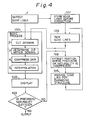
- Figure 4 is a flowchart for explaining the total operation from the detection of the edge lines of the two-dimensional scalar data to the output of the two-dimensional scalar data, including the steps 2 to 4 in Fig. 1, according to an embodiment of the present invention.
- reference 100 represents a basic process including the steps 2 to 4 shown in Fig. 1, 1 represents a edge line detecting step, 101 represents a storing step for storing edge line data before correction, 102 represents a total display process, 103 represents a precision or naturality judging process, 104 represents a step for extracting portions where the precision or naturality is insufficient, 105 represents a step for providing edge lines for expanding the structure of the two-dimensional scalar data, and 106 represents a step for forming data of new edge lines.
- the edge lines are detected by the edge line detecting step 1 illustrated in Fig. 1, and the detected edge lines are stored in a memory (not shown) in the step 101.
- the data of the detected edge lines are processed in the steps 2 to 4 according to the method described before so that the two-dimensional scalar data similar to the original two-dimensional scalar data is reconstructed.
- the reconstructed two-dimensional scalar data is displayed on, for example,a display surface in the total display process 102.
- an operator checks to determine whether there is an insufficiency in the precision or in the naturality.
- the precision is judged when the compressed data of the two-dimensional scalar data is to be transmitted.
- the naturality is judged when the two-dimensional scalar data is given by, for example a car designer, and when compressed data of the two-dimensional scalar data is to be stored. If there is an insufficiency, that portion is extracted in the step 104 for extracting a portion where the precision or the naturality is insufficient.
- a portion is, for example, a portion where the change of the luminance is comparatively loose so that no edge line is found, causing the above-mentioned insufficiency.
- step 105 for providing edge lines for expanding the structure data of a new edge line corresponding to the above-mentioned insufficient portion is provided. Then, in step 106, the data of the new edge line is combined with the data of the edge lines before correction stored in the step 101 so that data of a new edge line is obtained. The data of the new edge line is introduced to the basic process 100 so that the two-dimensional scalar data is again reconstructed.
- steps 100 to 106 are repeated until data having sufficient precision or sufficient naturality is obtained. If the reconstructed data is sufficient, it is output.
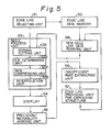
- FIG. 5 is a block diagram showing a scalar data processing apparatus according to an embodiment of the preset invention.
- 51 represents a edge line detecting unit
- 52 represents a edge line data storing memory for storing edge line data before correction
- 53 represents a basic process unit including a domain cutting unit 532, a ⁇ ⁇ determining unit 533, a data compressing unit 534, and an interpolation unit 535.
- Reference 54 is a display for effecting a total display process
- 55 represents a precision or naturality judging unit
- 56 represents a unit for extracting portions where the precision or naturality is insufficient
- 57 represents a unit for providing edge lines for expanding the structure of the two-dimensional scalar data
- 58 represents a unit for forming data of new edge lines.
- the following windows are provided so that display is carried out by a multi-window system in accordance with necessity. Namely, there are provided:
- the above windows ( i ), ( ii ), and ( iii ) are used to extract the values ⁇ (i,j) and their gradients on the edge lines.
- the window ( iv ) is used to compensate the parts where the above-mentioned compression and interpolation process are insufficient to obtain the desired reconstructed scalar data.
- the window ( v ) is used in the step 106 shown in Fig. 4.
- the windows ( vi ) and ( vii ) are used in the steps 100 to 106 in accordance with necessity.
- window operating functions the following functions are provided. Namely, there are provided:
- the present invention can be applied not only when the two-dimensional scalar data is to be transmitted but also when the two-dimensional scalar data is to be stored by, for example, a car designer.
Landscapes
- Engineering & Computer Science (AREA)
- Multimedia (AREA)
- Signal Processing (AREA)
- Image Processing (AREA)
Abstract
Description
- The present invention relates to a scalar data processing apparatus and a method for compressing two-dimensional scalar data and for reconstructing the compressed two-dimensional scalar data.
- It is desired to efficiently transmit and reconstruct two-dimensional scalar data ø (x,y) such as luminance data of a picture on a two-dimensional surface or concave-convex data of a relief formed on a wall surface, or to efficiently determine a two-dimensional function ø (x,y) of a curved surface of an object such as a car body when the outer shape of the object is to be determined.
- Conventionally, to transmit and reconstruct two-dimensional scalar data, or to determine the two-dimensional function, data of each pixel on the picture surface or each point on the desired body is used. This, however, requires that a tremendous amount of data be processed.
- Therefore, it has been desired to enable the reconstruction of two-dimensional scalar data with a small amount of data, smaller than the number of pixels or points on the picture surface.
- Reference can be made to U.S.Patent No. 4,908,698 issued on March 13, 1990, corresponding to Japanese Patent Application Nos. 62-133690 and 63-39284, filed by the same assignee of the present inventors. These applications are directed to providing a color picture synthesis technique in which, in a color picture transmission, a chrominance component of a given picture is separated into a lamellar component and a vortex component for transmission, and a synthesis of the color picture in combination with a luminance component in the above given picture is effected. This technique can be utilized in the present invention.
- In the above proposal, the chrominance component is expressed by a vector V, and when the Helmholtz theory is applied to the vector V, it is noted that the vector V can be expressed as:

- where L(x,y) is a scalar potential such as the luminance, and R · K is a vector potential having a direction expressed by a unit vector K in the direction of the Z axis.
- The lamellar component is the first item, i.e., grad L, in the above expression (1), and the vortex component is the second item, i.e., rot (R · K), in the above expression (1). By detecting and transmitting an edge line of the chrominance component by detecting only divergence V and rotation V which exceed predetermined threshold values which are the values on the edge line of the chrominance component of the picture, the chrominance component of the color picture for every point can be reconstructed by interpolation.
- The present invention was conceived from the above proposal with respect to the chrominance component.
- The present invention has an object to enable a reduction in the amount of data in the transmission or storing of two-dimensional scalar data by compressing two-dimensional data by the boundary value on the edge lines and by applying an interpolation by the use of the compressed data.
- As will be seen from the above proposal, in accordance with the Helmholtz theory, if a vector V does not have a vortex component, the vector V is expressed by only the lamellar component grad L. The gradient component of the two-dimensional scalar data ø such as luminance is a vector. Therefore, if the vector V can be expressed by a scalar potential grad ø , the Helmholtz theory is expressed as:

- An edge line of the scalar data is determined as a place where the divergence and rotation of the vector are greatly changed. The divergence of the vector in the expression (2) is

The rotation of the vector V in the expression (2) is
As a result of the above expressions (3) and (4), to detect the edge line of scalar data, since the rotation of the gradient ø is always zero, the edge line of the scalar data ø can be determined by detecting only the divergence of the gradient ø , i.e., the Laplacian △ ø , which exceeds the predetermined threshold value. Since the rotation of the vector V is always zero, it is not necessary to consider the rotation of the vector V. The Laplacian △ ø , the absolute value of which exceeds the predetermined threshold value can be detected by detecting the value ø and its gradient on the edge line. Once the value ø and its gradient on the edge line are given, the values ø at the other points can be estimated by interpolation because the values ø at the other points are changed loosely. - Based on the above-mentioned idea, there is provided, according to the present invention, a scalar data processing method and apparatus for compressing two-dimensional scalar data defined on a two-dimensional surface having a horizontal direction and a vertical direction and for reconstructing the two-dimensional scalar data based on the compressed data. The method comprises the step of detecting edge lines of the two-dimensional scalar data. The edge lines are detected in such a way that the change of the value of the two-dimensional scalar data between adjacent points on the two-dimensional surface is larger than a predetermined threshold value.
- The method further comprises the steps of cutting a domain along a horizontal line intersecting with the edge lines and between the edge lines; determining a function as an approximation of a Laplacian of the two-dimensional scalar data at each point in the cut domain; compressing the two-dimensional scalar data by replacing the two-dimensional scalar data at every point with scalar data at the edge lines, scalar data for providing gradients of the two-dimensional scalar data on the edge lines, and the function determined in the above step; and reconstructing the two-dimensional scalar data by interpolating the two-dimensional scalar data based on the scalar data at the edge lines, scalar data for providing gradients of the two-dimensional scalar data on the edge lines, and the function obtained in the above compressing step.
- The scalar data processing apparatus according to the present invention comprises an edge line detecting unit for detecting edge lines of the two-dimensional scalar data; a domain cutting unit for cutting a domain on a horizontal line intersecting with the edge lines and between the edge lines; a function determining unit for determining a function as an approximation of a Laplacian of the two-dimensional scalar data at each point in the cut domain; a compressing unit for compressing the two-dimensional scalar data by replacing the two-dimensional scalar data at every point with scalar data at the edge lines, scalar data for providing gradients of the two-dimensional scalar data on the edge lines, and the function determined in the above compressing unit ; and a reconstructing unit for reconstructing the two-dimensional scalar data by interpolating the two-dimensional scalar data based on the scalar data at the edge lines, scalar data for providing gradients of the two-dimensional scalar data on the edge lines, and the function.
-
- Figure 1 is a flowchart showing the principle operation of the scalar data processing according to an embodiment of the present invention;
- Fig. 2A shows equations used for effecting interpolation according to an embodiment of the present invention;
- Fig. 2B shows a display surface for explaining the interpolation process according to an embodiment of the present invention;
- Fig. 3A shows a display surface for explaining the interpolation process according to another embodiment of the present invention;
- Fig. 3B shows equations used for effecting interpolation in the embodiment shown in Fig. 3A;
- Fig. 4 is a flowchart for explaining the total operation from the detection of the edge lines of the two-dimensional scalar data to the output of the two-dimensional scalar data, including the
steps 2 to 4 in Fig. 1, according to an embodiment of the present invention; and - Fig. 5 is a block diagram showing a scalar data processing apparatus according to an embodiment of the present invention.
- Figure 1 is a flowchart showing the principle operation of the scalar data processing according to an embodiment of the present invention. The right hand side of the flowchart represents a picture on a
display 10. - In the right-hand side figure in Fig. 1,
reference 10 represents a display in which "i" represents an x coordinate in the horizontal direction and "j" represents a y coordinate in the longitudinal direction, 11-1 and 11-2 represent the edge lines, 12 represents a domain cut by the edge lines 11-1 and 11-2, 13-1 and 13-2 represent points on the edge lines 11-1 and 11-2 and on thehorizontal scanning line 17, 14-1 and 14-2 represent points on thehorizontal scanning line 17 adjacent to the points 13-1 and 13-2 on the edge lines 11-1 and 11-2, 15 represents a point within thecut domain 12 which is the subject for the interpolation, 16-1, 16-2, 16-3, and 16-4 represent points adjacent to thepoint - In the figure,
reference 1 is a step for detecting boundaries 11-1 and 11-2 (referred to as edge lines) of two-dimensional scalar data such as luminance of a picture image when the picture image is the subject to be processed. The edgeline detecting step 1 is carried out by utilizing appropriate means as disclosed in U.S.Patent No. 4,908,698 corresponding to Japanese Patent Application No. 63-39284, and therefore a practical explanation thereof is omitted here. -
Reference 2 is a step for cutting thedomain 12 on ahorizontal line 17 between the edge lines 11-1 and 11-2 detected by the edgeline detecting step 1. -
Reference 3 is a step for determining a Laplacian △ ø corresponding to the scalar data ø within the domain cut as above by approximating the Laplacian △ ø to be a function f(i) with respect to the coordinate on the horizontal scanning line. Namely,the Laplacian △ ø is approximated as a function f(i) which may be a constant value including zero, a linear function of the coordinate i, a quadratic function of the coordinate i, or a three-dimensional function of the coordinate i, in accordance with the desired precision. In theLaplacian determining step 3, cooefficients in the function are determined by, for example, the method of least squares. -
Reference 4 is a step for compressing data by extracting the values ø (i,j) on the edge lines 11-1 and 11-2, values ø (i,j) at points adjacent to the points on the edge lines 11-1 and 11-2 for providing values of grad ø (i,j) on the edge lines, and the above-mentioned function f(i) as the Laplacian △ ø within thecut domain 12. -
Reference 5 is a step of interpolation to obtain the values ø (i,j) of the respective points on thehorizontal scanning line 17 and within thecut domain 12 to reconstruct the original two-dimensional scalar data ø . - In the
domain cutting step 2, the edge lines 11-1 and 11-2 are shown on thedisplay 10. Adomain 12 on thehorizontal scanning line 17 is cut by the edge lines 11-1 and 11-2. - In the △
ø determining step 3, a Laplacian △ ø is calculated at each point on each horizontal scanning line by the use of the values of the scalar data ø on the edge lines 11-1 and 11-2 and its gradient on the contour lines 11-1 and 11-2 and by the use of the scalar data ø in thecut domain 12. Within thecut domain 12, the change of the Laplacian △ ø is considered to be loose. Therefore, the Laplacian △ ø can be approximated as a simple function f(i). Since there are four boundary values, i.e., the two scalar data on the edge lines and the two values of gradients on the edge lines, the function f(i) can be expressed by at maximum a three-dimensional function with respect to the coodinate value i on the horizontal scanning line. - Accordingly, as the above function f(i), the following function may be applied.
- ( i )
- △ ø =f(i) =const
- ( ii )
- △ ø =f(i)=ai+b
- ( iii )
- △ ø =f(i)=ai²+bi+c
- ( iv )
- △ ø =f(i)=ai³+bi²+ci+d
- The constant value in the equation ( i ), the coefficients a and b in the equation ( ii ), the coefficients a, b, and c in the equation ( iii ), or the coefficients a, b, c, and d are determined in such a way that the function f(i) is as close as possible to the calculated Laplacian △ ø at each point by, for example, means of the method of least squares. According to an experiment performed by the inventors, even when an approximation is taken so that

- When a higher degree of approximation is required, an approximation of higher accuracy is carried out by the use of the equation ( i ), ( ii ), ( iii ) or ( iv ) .
- In the
data compression step 4, for eachhorizontal scanning line 17, the values ø (i,j) at the points 13-1 and 13-2 on the edge lines 11-1 and 11-2, the values ø (i,j) at the points 14-1 and 14-2 adjacent to the points 13-1 and 13-2 for calculating the gradient on the edge lines 11-1 and 11-2, and the above-mentioned function f(i) are used as compressed data. The compressed data is transmitted to a receiving side or is stored for reconstruction. Of course, the adjacent points 14-1 and 14-2 for obtaining the gradients on the edge lines are not restricted to two, but adjacent points on the edge lines 11-1 and 11-2 may also be taken into account. The values ø (i,j) and their gradients on the edge lines, however, do not greatly change in general. Therefore, it is sufficient to take into account only the above-mentioned two points 14-1 and 14-2 to obtain the gradient on the edge lines. - In the
interpolation step 5, the value ø (i,j) at each point within thecut domain 12 on thehorizontal scanning line 17 is obtained by interpolation to reconstruct the original two-dimensional scalar data. Namely, to obtain the value ø (i,j) at eachpoint 15 within thedomain 12, interpolation is carried out in accordance with a successive approximation by the use of the compressed data, i.e., the boundary values ø (i,j) on the edge lines 11-1 and 11-2, the boundary values grad ø (i,j) on the edge lines 11-1 and 11-2, and the above-mentioned function f(i). - According to the successive approximation used to obtain the value ø (i,j) at a
point 15 within thecut domain 12, roughly determined values ø (i,j) at points 16-1, 16-2, 16-3, and 16-4 adjacent to thepoint 15 and a roughly determined value ø (i,j) at thepoint 15 are utilized to calculate a rough Laplacian △ ø (i,j). The interpolation process is carried out in such a way that the above-mentioned function f(i) is satisfied as long as possible. - Figure 2A shows equations for carrying out the interpolation process according to an embodiment of the present invention, and Fig. 2B shows a display for explaining the interpolation process.
- As shown in Fig. 2A, the equation (A), i.e., △ ø = f(i), and the equation (B), i.e., △ øk=øk(i+1,j)+øk(i,j+1)+øk(i-1,j)+øk(i,j-1)-4øk(i,j), where the suffix k represents the number of times of estimation, are utilized for interpolation.
- Generally, the Laplacian △ ø can be expressed by the equation (B) shown in Fig. 2A. This equation can be understood from the following calculations.


Similarly,

- First, based on the compressed data, the values ø (i,j) at the points 13-1 to 13-6 on the edge lines 11-1 and 11-2 are known. Also, the values ø (i,j) at the points 14-1 to 14-6 adjacent to the points 13-1 to 13-6 are known because the gradient ø (i,j) on the edge lines are included in the compressed data. Based on these values ø (i,j) at the points 13-1 to 13-6 and the values ø (i,j) at the points 14-1 to 14-6, the value at each point within the
cut domain 12 is roughly estimated. For, example, the first estimation is carried out in such a way that the values of the points between the points 14-1 and 14-2 are assumed to be linearly changed. By this estimation, it is assumed that the estimated value at each point within the cut domains 12-1 to 12-3 is expressed as ø ₁(i,j). Then, the estimated Laplacian △ ø ₁(i,j) is calculated in accordance with the equation (B), where k=1. - Next, the estimated Laplacian △ ø ₁(i,j) and the function f(i) are compared to determine whether the estimated value △ ø ₁(i,j) satisfies the function f(i) . To this end, an error E₁ is calculated, where

- When the absolute value of the error E₁ is larger than a predetermined threshold value, the first estimated values ø ₁(i,j) at each point are corrected to secondary estimated values ø ₂(i,j) in the following manner.

- By using the secondary estimated values, a similar calculation is made according to the equation (B), i.e., △ø₂(i,j)=ø₂(i+1,j)+ø₂(i,j+1)+ø₂(i-1,j)+ø₂(i,j-1)-4ø₂(i,j). Then, if an error E₂ = f(i)-△ø₂(i,j) is larger than the predetermined threshold value, the secondary estimated values ø ₂(i,j) at each point are corrected to third estimated values in a way similar to the above. Namely, by using the above relation, the correction is made and the value ø (i,j) at each point within the cut domain is converged so that the above-mentioned function f(i) is satisfied within the predetermined threshold value. As a result, the value ø (i,j) at each point on the two-dimensional surface can be reconstructed.
- Figure 3A shows a display for explaining the interpolation process according to another embodiment of the present invention. In the illustrated case, the Laplacian △ ø can also be expressed by the equation (D) shown in Fig. 3B. This equation can be undersood by the following calculations.


Similarly,

- First, based on the compressed data, the values ø (i,j) at the points 13-1 to 13-6 on the edge lines 11-1 and 11-2 are known. Also, the values ø (i,j) at the points 14-1 to 14-6 adjacent to the points 13-1 to 13-6 are known as explained before. Based on these values ø (i,j) at the points 13-1 to 13-6 and the values ø (i,j) at the points 14-1 to 14-6, the value at each point within the cut domain is roughly estimated in the same way as described with reference to Fig. 2B. By this estimation, it is assumed that the estimated value at each point within the cut domains 12-1 to 12-3 is expressed as ø ₁(i,j). Then, the estimated Laplacian △ ø ₁(i,j) is calculated in accordance with the equation (D).
- Next, the estimated Laplacian △ ø ₁(i,j) and the function f(i) are compared to determine whether the estimated value △ ø ₁(i,j) satisfies the function f(i) . To this end, an error E₁ is calculated, where

- When the absolute value of the error E is larger than a predetermined threshold value, the first estimated value ø ₁(i,j) at each point is corrected to a secondary estimated value ø ₂(i,j) in the following manner.

- By using the secondary estimated values, a similar calculation is carried out according to the equation (D), i.e.,△ø₂(i,j)=2ø₂(i,j)-2ø₂(i-1,j)+ø₂(i-1,j)-2ø₂(i,j-1)+ø₂(i,j-2). Then, if an error E₂=f(i)-△ø₂(i,j) is greater than the predetermined threshold value, the secondary estimated value ø ₂(i,j) at each point is corrected to a third estimated value in the similar way as above. Namely, by using the above relation, the correction is made and the value ø (i,j) at each point within the cut domain is converged so that the above-mentioned function f(i) is satisfied within the predetermined threshold value.
- Figure 4 is a flowchart for explaining the total operation from the detection of the edge lines of the two-dimensional scalar data to the output of the two-dimensional scalar data, including the
steps 2 to 4 in Fig. 1, according to an embodiment of the present invention. - In the figure,
reference 100 represents a basic process including thesteps 2 to 4 shown in Fig. 1, 1 represents a edge line detecting step, 101 represents a storing step for storing edge line data before correction, 102 represents a total display process, 103 represents a precision or naturality judging process, 104 represents a step for extracting portions where the precision or naturality is insufficient, 105 represents a step for providing edge lines for expanding the structure of the two-dimensional scalar data, and 106 represents a step for forming data of new edge lines. - Before carrying out the
basic process 100, the edge lines are detected by the edgeline detecting step 1 illustrated in Fig. 1, and the detected edge lines are stored in a memory (not shown) in thestep 101. - In the
basic process 100, the data of the detected edge lines are processed in thesteps 2 to 4 according to the method described before so that the two-dimensional scalar data similar to the original two-dimensional scalar data is reconstructed. The reconstructed two-dimensional scalar data is displayed on, for example,a display surface in thetotal display process 102. - In the precision or
naturality judging process 103, in view of the illustrated picture image of the two-dimensional scalar data, an operator, for example, checks to determine whether there is an insufficiency in the precision or in the naturality. The precision is judged when the compressed data of the two-dimensional scalar data is to be transmitted. The naturality is judged when the two-dimensional scalar data is given by, for example a car designer, and when compressed data of the two-dimensional scalar data is to be stored. If there is an insufficiency, that portion is extracted in thestep 104 for extracting a portion where the precision or the naturality is insufficient. Such a portion is, for example, a portion where the change of the luminance is comparatively loose so that no edge line is found, causing the above-mentioned insufficiency. - In the
step 105 for providing edge lines for expanding the structure, data of a new edge line corresponding to the above-mentioned insufficient portion is provided. Then, instep 106, the data of the new edge line is combined with the data of the edge lines before correction stored in thestep 101 so that data of a new edge line is obtained. The data of the new edge line is introduced to thebasic process 100 so that the two-dimensional scalar data is again reconstructed. - These new edge lines play a role to correct values of ø (i,j) to satisfy the designer. In this case, these new edge lines gives correction lines which are virtual lines.
- The above-mentioned
steps 100 to 106 are repeated until data having sufficient precision or sufficient naturality is obtained. If the reconstructed data is sufficient, it is output. - Figure 5 is a block diagram showing a scalar data processing apparatus according to an embodiment of the preset invention. In the figure, 51 represents a edge line detecting unit, 52 represents a edge line data storing memory for storing edge line data before correction, and 53 represents a basic process unit including a
domain cutting unit 532, a △ø determining unit 533, adata compressing unit 534, and aninterpolation unit 535.Reference 54 is a display for effecting a total display process, 55 represents a precision or naturality judging unit, 56 represents a unit for extracting portions where the precision or naturality is insufficient, 57 represents a unit for providing edge lines for expanding the structure of the two-dimensional scalar data, and 58 represents a unit for forming data of new edge lines. - The operation of the scalar data processing apparatus shown in Fig. 5 is already described with reference to Fig. 4.
- In the present invention, the following windows are provided so that display is carried out by a multi-window system in accordance with necessity. Namely, there are provided:
- ( i ) a edge line display window
- ( ii ) a edge line circumferential data display window
- ( iii ) a data display window
- ( iv ) a texture definition/superimposition display window
- ( v ) a new edge line display window
- ( vi ) a process history display window and
- ( vii ) a moving picture/animation display window.
- The above windows ( i ), ( ii ), and ( iii ) are used to extract the values ø (i,j) and their gradients on the edge lines. The window ( iv ) is used to compensate the parts where the above-mentioned compression and interpolation process are insufficient to obtain the desired reconstructed scalar data. The window ( v ) is used in the
step 106 shown in Fig. 4. The windows ( vi ) and ( vii ) are used in thesteps 100 to 106 in accordance with necessity. - Also, as window operating functions, the following functions are provided. Namely, there are provided:
- ( i ) edge line definition/correction function
- ( ii ) data definition/correction function
- ( iii ) definition of interpolation data output display-structure expansion edge line/correction function
- ( iv ) texture definition/correction function
- ( v ) definition of continuousness of a moving picture/correction function and
- ( vi ) texture definition in a domain/correction function.
- From the foregoing description, it is apparent that, according to the present invention, the data value ø (i,j) of two-dimensional scalar data at each point can be reconstructed in such a way that

- The present invention can be applied not only when the two-dimensional scalar data is to be transmitted but also when the two-dimensional scalar data is to be stored by, for example, a car designer.
Claims (16)
- A scalar data processing method for compressing two-dimensional scalar data defined on a two-dimensional surface having a horizontal direction (i) and a vetical direction (j) and for reconstructing said two-dimensional scalar data based on said compressed data, comprising the steps of:
detecting edge lines (11-1,11-2) of said two-dimensional scalar data (ø (i,j)), said edge lines (11-1,11-2) being detected in such a way that a change in the value of said two-dimensional scalar data between adjacent points on said two-dimensional surface is larger than a predetermined threshold value;
cutting a domain (12) on a horizontal line (17) intersecting said edge lines and between said edge lines (11-1,11-2);
determining a function (f(i)) as an approximation of a Laplacian of said two-dimensional scalar data (ø (i,j)) at each point in said cut domain (12);
compressing said two-dimensional scalar data (ø (i,j)) by replacing said two-dimensional scalar data at every point with scalar data at said edge lines (11-1,11-2), scalar data for providing gradients of said two-dimensional scalar data on said edge lines, and said function (f(i)); and
reconstructing said two-dimensional scalar data by interpolating said two-dimensional scalar data based on said scalar data at said edge lines (11-1,11-2), scalar data for providing gradients of said two-dimensional scalar data on said edge lines, and said function (f(i)) obtained in said compressing step. - A scalar data processing method as claimed in claim 1, wherein said edge line detecting step comprises a step for detecting data of said edge lines.
- A scalar data processing method as claimed in claim 2, wherein said domain cutting step comprises a step for cutting said domain based on said data of said edge lines.
- A scalar data processing method as claimed in claim 1, wherein in said step for determining a function (f(i)), the function is assumed as zero.
- A scalar data processing method as claimed in claim 1, wherein in said step for determining a function (f(i)), the function is assumed as a constant value.
- A scalar data processing method as claimed in claim 1, wherein in said step for determining a function (f(i)), the function is assumed as a linear function with respect to a coordinate of the horizontal line.
- A scalar data processing method as claimed in claim 1, wherein in said step for determining a function (f(i)), the function is assumed as a secondary order function with respect to a coordinate of the horizontal line.
- A scalar data processing method as claimed in claim 1, wherein in said step for determining a function (f(i)), the function is assumed as a third order function with respect to a coordinate of the horizontal line.
- A scalar data processing method as claimed in claim 1, wherein in said step for determining a function (f(i)), the function is determined by the method of least-square approximation with respect to the function and the Laplacian of said two-dimensional scalar data at each point on said two-dimensional surface.
- A scalar data processing method as claimed in claim 1, wherein in said step for compressing said two-dimensional scalar data (ø (i,j)), said replaced data is transmitted from a transmitting side to a receiving side when said two-dimensional scalar data is to be transmitted.
- A scalar data processing method as claimed in claim 1, wherein in said step for compressing said two-dimensional scalar data (ø (i,j)), said replaced data is transmitted from a transmitting side to a receiving side, and said step for interpolation is carried out in said receiving side.
- A scalar data processing method as claimed in claim 1, wherein in said step for compressing said two-dimensional scalar data (ø (i,j)), said replaced data is stored for reconstructing the original two-dimensional scalar data by said interpolation step.
- A scalar data processing method as claimed in claim 1, wherein in said step for reconstructing said two-dimensional scalar data, said interpolation is carried out by successive approximation in such a way that, at first approximation, the approximated two-dimensional scalar data is determined based on the values of said edge lines and the values which give the gradients of the two-dimensional scalar data, and then the difference between said function and the value (△ ø K(i,j)) of a Laplacian of approximated two-dimensional scalar data at each point comes within a predetermined threshold value.
- A scalar data processing method as claimed in claim 13, wherein in said step for reconstructing said two-dimensional scalar data, said value (△ ø K(i,j)) of a Laplacian of approximated two-dimensional scalar data at each point is expressed as △øK(i,j)=øK(i+1,j)+øK(i,j+1)+øK(i-1,j)+øK(i,j-1)-4øK(i,j), where i is an x coordinate, j is a y coordinate, and k is the number of succesive approximations.
- A scalar data processing method as claimed in claim 13, wherein in said step for reconstructing said two-dimensional scalar data, said value (△ ø K(i,j)) of a Laplacian of approximated two-dimensional scalar data at each point is expressed as △øK(i,j)=2øK(i,j)-2øK(i-1,j)+øK(i-2,j)-2øK(i,j-1)+øK(i,j-2), where i is an x coordinate, j is a y coordinate, and k is the number of succesive approximations.
- A scalar data processing apparatus for compressing two-dimensional scalar data defined on a two-dimensional surface having a horizontal direction (i) and a vertical direction (j) and for reconstructing said two-dimensional scalar data based on said compressed data, comprising:
edge line detecting means (51) for detecting edge lines of said two-dimensional scalar data (ø (i,j)), said edge lines (11-1,11-2) being detected in such a way that the change of the value of said two-dimensional scalar data between adjacent points on said two-dimensional surface is larger than a predetermined threshold value;
domain cutting means (532) for cutting a domain (12) on a horizontal line (17) intersecting with said edge lines and between said edge lines (11-1,11-2);
function determining means (533) for determining a function (f(i)) as an approximation of a Laplacian of said two-dimensional scalar data (ø (i,j)) at each point in said cut domain (12);
compressing means (534) for compressing said two-dimensional scalar data (ø (i,j)) by replacing said two-dimensional scalar data at every point with scalar data at said edge lines (11-1,11-2), scalar data for providing gradients of said two-dimensional scalar data on said edge lines, and said function (f(i)); and
reconstructing means (535) for reconstructing said two-dimensional scalar data by interpolating said two-dimensional scalar data based on said scalar data at said edge lines (11-1,11-2), scalar data for providing gradients of said two-dimensional scalar data on said edge lines, and said function (f(i)).
Applications Claiming Priority (2)
| Application Number | Priority Date | Filing Date | Title |
|---|---|---|---|
| JP66149/90 | 1990-03-16 | ||
| JP6614990A JP3072766B2 (en) | 1990-03-16 | 1990-03-16 | Scalar data processing method |
Publications (3)
| Publication Number | Publication Date |
|---|---|
| EP0447328A2 true EP0447328A2 (en) | 1991-09-18 |
| EP0447328A3 EP0447328A3 (en) | 1994-01-05 |
| EP0447328B1 EP0447328B1 (en) | 1998-10-07 |
Family
ID=13307522
Family Applications (1)
| Application Number | Title | Priority Date | Filing Date |
|---|---|---|---|
| EP19910400712 Expired - Lifetime EP0447328B1 (en) | 1990-03-16 | 1991-03-15 | Scalar data processing method and apparatus |
Country Status (4)
| Country | Link |
|---|---|
| US (1) | US5148501A (en) |
| EP (1) | EP0447328B1 (en) |
| JP (1) | JP3072766B2 (en) |
| DE (1) | DE69130302T2 (en) |
Families Citing this family (14)
| Publication number | Priority date | Publication date | Assignee | Title |
|---|---|---|---|---|
| US5537494A (en) * | 1990-05-29 | 1996-07-16 | Axiom Innovation Limited | Video image data encoding and compression system using edge detection and luminance profile matching |
| JP2585874B2 (en) * | 1991-03-18 | 1997-02-26 | 富士通株式会社 | Edge detection method for color images |
| US5818970A (en) * | 1991-04-26 | 1998-10-06 | Canon Kabushiki Kaisha | Image encoding apparatus |
| US5416855A (en) * | 1992-03-03 | 1995-05-16 | Massachusetts Institute Of Technology | Image compression method and apparatus |
| DE69312132T2 (en) * | 1992-03-17 | 1998-01-15 | Sony Corp | Image compression device |
| US6195461B1 (en) * | 1992-12-17 | 2001-02-27 | Sony Corporation | Dynamic image processing apparatus and method |
| JP2938739B2 (en) * | 1993-02-26 | 1999-08-25 | 富士通株式会社 | Moving image processing device |
| US5982990A (en) * | 1995-07-20 | 1999-11-09 | Hewlett-Packard Company | Method and apparatus for converting color space |
| US5748176A (en) * | 1995-07-20 | 1998-05-05 | Hewlett-Packard Company | Multi-variable colorimetric data access by iterative interpolation and subdivision |
| US20010004838A1 (en) * | 1999-10-29 | 2001-06-28 | Wong Kenneth Kai | Integrated heat exchanger system for producing carbon dioxide |
| US6853736B2 (en) * | 2000-02-04 | 2005-02-08 | Canon Kabushiki Kaisha | Image processing apparatus, image processing method and storage medium |
| US7167602B2 (en) * | 2001-07-09 | 2007-01-23 | Sanyo Electric Co., Ltd. | Interpolation pixel value determining method |
| TWI366181B (en) * | 2007-06-12 | 2012-06-11 | Au Optronics Corp | Method and apparatus for image enlargement and enhancement |
| US11143545B2 (en) | 2019-02-12 | 2021-10-12 | Computational Systems, Inc. | Thinning of scalar vibration data |
Family Cites Families (7)
| Publication number | Priority date | Publication date | Assignee | Title |
|---|---|---|---|---|
| US4648120A (en) * | 1982-07-02 | 1987-03-03 | Conoco Inc. | Edge and line detection in multidimensional noisy, imagery data |
| US4910786A (en) * | 1985-09-30 | 1990-03-20 | Eichel Paul H | Method of detecting intensity edge paths |
| AU583202B2 (en) * | 1987-02-06 | 1989-04-20 | Fujitsu Limited | Method and apparatus for extracting pattern contours in image processing |
| CA1286767C (en) * | 1987-05-29 | 1991-07-23 | Hajime Enomoto | Color picture image processing system for separating color picture imageinto pixels |
| US4849914A (en) * | 1987-09-22 | 1989-07-18 | Opti-Copy, Inc. | Method and apparatus for registering color separation film |
| JPH01286676A (en) * | 1988-05-13 | 1989-11-17 | Fujitsu Ltd | Picture data compressing system |
| US5014134A (en) * | 1989-09-11 | 1991-05-07 | Aware, Inc. | Image compression method and apparatus |
-
1990
- 1990-03-16 JP JP6614990A patent/JP3072766B2/en not_active Expired - Lifetime
-
1991
- 1991-03-08 US US07/666,712 patent/US5148501A/en not_active Expired - Lifetime
- 1991-03-15 EP EP19910400712 patent/EP0447328B1/en not_active Expired - Lifetime
- 1991-03-15 DE DE69130302T patent/DE69130302T2/en not_active Expired - Fee Related
Also Published As
| Publication number | Publication date |
|---|---|
| JP3072766B2 (en) | 2000-08-07 |
| EP0447328B1 (en) | 1998-10-07 |
| DE69130302D1 (en) | 1998-11-12 |
| JPH03267879A (en) | 1991-11-28 |
| US5148501A (en) | 1992-09-15 |
| EP0447328A3 (en) | 1994-01-05 |
| DE69130302T2 (en) | 1999-03-04 |
Similar Documents
| Publication | Publication Date | Title |
|---|---|---|
| EP0447328A2 (en) | Scalar data processing method and apparatus | |
| EP0720377B1 (en) | Method for detecting motion vectors for use in a segmentation-based coding system | |
| JP2523369B2 (en) | Method and apparatus for detecting motion of moving image | |
| EP0447068B1 (en) | Motion image data compression system | |
| KR100306948B1 (en) | Mosaic based image processing system and method for processing images | |
| US5734743A (en) | Image processing method and apparatus for block-based corresponding point extraction | |
| EP1303839B1 (en) | System and method for median fusion of depth maps | |
| WO2002045003A1 (en) | Techniques and systems for developing high-resolution imagery | |
| EP0726543A2 (en) | Image processing method and apparatus therefor | |
| GB2300083A (en) | Fractal image compression | |
| EP0643538A2 (en) | Motion vector detecting apparatus and methods | |
| CA2299578A1 (en) | A contour extraction apparatus, a method thereof, and a program recording medium | |
| US7522189B2 (en) | Automatic stabilization control apparatus, automatic stabilization control method, and computer readable recording medium having automatic stabilization control program recorded thereon | |
| Park et al. | A mesh-based disparity representation method for view interpolation and stereo image compression | |
| US6285712B1 (en) | Image processing apparatus, image processing method, and providing medium therefor | |
| FR2615981A1 (en) | METHOD AND APPARATUS FOR OBTAINING INSTANT INVERSE VALUES OF HOMOGENEOUS COORDINATES W FOR USE IN IMAGE RESTITUTION ON DISPLAY BODY | |
| US6032167A (en) | Data processing circuit adapted for use in pattern matching | |
| EP0770974A1 (en) | Motion picture reconstruction method and apparatus | |
| JP2856661B2 (en) | Density converter | |
| US6836562B2 (en) | Method for determining the shape of objects directly from range images | |
| Pardas et al. | Motion and region overlapping estimation for segmentation-based video coding | |
| Jang et al. | Surface offsetting using distance volumes | |
| Tsai et al. | A curve evolution approach to medical image magnification via the Mumford-Shah functional | |
| JPH10255049A (en) | Image processing method using block matching | |
| JP2878580B2 (en) | Hierarchical motion vector detection method |
Legal Events
| Date | Code | Title | Description |
|---|---|---|---|
| PUAI | Public reference made under article 153(3) epc to a published international application that has entered the european phase |
Free format text: ORIGINAL CODE: 0009012 |
|
| AK | Designated contracting states |
Kind code of ref document: A2 Designated state(s): DE FR GB |
|
| PUAL | Search report despatched |
Free format text: ORIGINAL CODE: 0009013 |
|
| AK | Designated contracting states |
Kind code of ref document: A3 Designated state(s): DE FR GB |
|
| 17P | Request for examination filed |
Effective date: 19940218 |
|
| 17Q | First examination report despatched |
Effective date: 19960131 |
|
| GRAG | Despatch of communication of intention to grant |
Free format text: ORIGINAL CODE: EPIDOS AGRA |
|
| GRAG | Despatch of communication of intention to grant |
Free format text: ORIGINAL CODE: EPIDOS AGRA |
|
| GRAG | Despatch of communication of intention to grant |
Free format text: ORIGINAL CODE: EPIDOS AGRA |
|
| GRAG | Despatch of communication of intention to grant |
Free format text: ORIGINAL CODE: EPIDOS AGRA |
|
| GRAH | Despatch of communication of intention to grant a patent |
Free format text: ORIGINAL CODE: EPIDOS IGRA |
|
| GRAH | Despatch of communication of intention to grant a patent |
Free format text: ORIGINAL CODE: EPIDOS IGRA |
|
| GRAA | (expected) grant |
Free format text: ORIGINAL CODE: 0009210 |
|
| AK | Designated contracting states |
Kind code of ref document: B1 Designated state(s): DE FR GB |
|
| REF | Corresponds to: |
Ref document number: 69130302 Country of ref document: DE Date of ref document: 19981112 |
|
| RHK2 | Main classification (correction) |
Ipc: H04N 7/13 |
|
| ET | Fr: translation filed | ||
| PLBE | No opposition filed within time limit |
Free format text: ORIGINAL CODE: 0009261 |
|
| STAA | Information on the status of an ep patent application or granted ep patent |
Free format text: STATUS: NO OPPOSITION FILED WITHIN TIME LIMIT |
|
| 26N | No opposition filed | ||
| REG | Reference to a national code |
Ref country code: GB Ref legal event code: IF02 |
|
| PGFP | Annual fee paid to national office [announced via postgrant information from national office to epo] |
Ref country code: GB Payment date: 20090311 Year of fee payment: 19 |
|
| PGFP | Annual fee paid to national office [announced via postgrant information from national office to epo] |
Ref country code: DE Payment date: 20090313 Year of fee payment: 19 |
|
| PGFP | Annual fee paid to national office [announced via postgrant information from national office to epo] |
Ref country code: FR Payment date: 20090316 Year of fee payment: 19 |
|
| GBPC | Gb: european patent ceased through non-payment of renewal fee |
Effective date: 20100315 |
|
| REG | Reference to a national code |
Ref country code: FR Ref legal event code: ST Effective date: 20101130 |
|
| PG25 | Lapsed in a contracting state [announced via postgrant information from national office to epo] |
Ref country code: FR Free format text: LAPSE BECAUSE OF NON-PAYMENT OF DUE FEES Effective date: 20100331 |
|
| PG25 | Lapsed in a contracting state [announced via postgrant information from national office to epo] |
Ref country code: DE Free format text: LAPSE BECAUSE OF NON-PAYMENT OF DUE FEES Effective date: 20101001 |
|
| PG25 | Lapsed in a contracting state [announced via postgrant information from national office to epo] |
Ref country code: GB Free format text: LAPSE BECAUSE OF NON-PAYMENT OF DUE FEES Effective date: 20100315 |