EP0216657B1

EP0216657B1 - Method of modulating the velocity effect of movable parts of a body in a density measurement by nuclear magnetic resonance

Info

Publication number: EP0216657B1
Application number: EP19860401788
Authority: EP
Inventors: Patrick Le Roux
Original assignee: General Electric CGR SA
Current assignee: General Electric CGR SA
Priority date: 1985-08-13
Filing date: 1986-08-08
Publication date: 1990-08-01
Anticipated expiration: 2006-08-08
Also published as: EP0216657A1; DE3673107D1

Description

La présente invention a pour objet un procédé de modulation de l'effet de la vitesse des parties mobiles d'un corps dans une mesure de densité par résonance magnétique nucléaire (RMN) ainsi que la mise en oeuvre du procédé pour en déduire la vitesse des parties mobiles concernées. L'invention trouve son application particulièrement dans le domaine médical où les corps examinés sont des corps humains et où les parties mobiles sont des cellules du sang circulant dans des veines ou des artères ou des organes mobiles tels que le muscle cardiaque. Dans cette application, l'invention peut même plus particulièrement être mise en oeuvre avec un procédé d'imagerie pour donner une image représentative de la répartition des vitesses des parties mobiles dans une coupe du corps examiné.The subject of the present invention is a method of modulating the effect of the speed of the moving parts of a body in a density measurement by nuclear magnetic resonance (NMR) as well as the implementation of the method to deduce therefrom the speed of moving parts concerned. The invention finds its application particularly in the medical field where the bodies examined are human bodies and where the moving parts are blood cells circulating in veins or arteries or moving organs such as the heart muscle. In this application, the invention can even more particularly be implemented with an imaging method to give an image representative of the distribution of the speeds of the moving parts in a section of the body examined.

En effet, l'imagerie par résonance magnétique nucléaire se développe principalement comme moyen de diagnostic médical. Elle permet la visualisation des structures internes tissulaires avec un contraste et une résolution jamais atteints simultanément par les autres procédés d'imagerie. Pour obtenir une image par résonance magnétique nucléaire d'une coupe d'un corps avec différenciation des caractéristiques tissulaires de ce corps, on utilise la propriété qu'ont certaines particules, comme les protons, d'orienter leur moment magnétique en acquérant de l'énergie lorsqu'ils sont placés dans un champ magnétique principal constant Bo. Une zone particulière d'un corps contenant des particules présente alors un moment magnétique global que l'on peut faire basculer selon une orientation donnée, perpendiculaire ou parallèle au champ Bo, en induisant une résonance par émission d'un champ magnétique radiofréquence perpendiculaire au champ principal.Indeed, nuclear magnetic resonance imaging is mainly developed as a means of medical diagnosis. It allows visualization of internal tissue structures with a contrast and resolution never achieved simultaneously by other imaging methods. To obtain a nuclear magnetic resonance image of a section of a body with differentiation of the tissue characteristics of this body, we use the property that certain particles, such as protons, have to orient their magnetic moment by acquiring energy when placed in a constant main magnetic field Bo. A particular zone of a body containing particles then presents an overall magnetic moment which can be tilted according to a given orientation, perpendicular or parallel to the field Bo, by inducing a resonance by emission of a radiofrequency magnetic field perpendicular to the field main.

Toutes les particules possédant alors un moment magnétique, tournant à une vitesse de précession dite de Larmor, tendent à retrouver l'orientation initiale parallèle à Bo en émettant un signal radiofréquence à la fréquence de résonance caractéristique de Bo et de la particule. Ce signal peut être capté par une antenne de réception. La durée de retour à l'équilibre du moment magnétique global d'une région considérée et la décroissance du signal dépendent de deux facteurs importants : l'interaction spin- réseau et l'interaction spin-spin des particules avec la matière environnante. Ces deux facteurs conduisent à la définition de deux temps de relaxation caractéristiques du tissu et dits respectivement T₁ et T₂. Une région considérée d'un objet émet donc un signal dont l'intensité dépend de Ti, de T₂, de la densité de particules dans la région, et du temps qui s'est écoulé depuis l'excitation radiofréquence.All the particles then having a magnetic moment, rotating at a so-called Larmor precession speed, tend to find the initial orientation parallel to Bo by emitting a radiofrequency signal at the resonance frequency characteristic of Bo and of the particle. This signal can be received by a receiving antenna. The duration of return to equilibrium of the global magnetic moment of a region considered and the decrease of the signal depend on two important factors: the spin-network interaction and the spin-spin interaction of the particles with the surrounding matter. These two factors lead to the definition of two relaxation times characteristic of the tissue and called T ₁ and T _{2 respectively} . A region considered of an object therefore emits a signal whose intensity depends on Ti, T ₂ , the density of particles in the region, and the time that has elapsed since the radio frequency excitation.

Si le champ orientateur est parfaitement homogène, des particules mobiles dans une région considérée émettent en réponse un signal identique à celui des particules fixes de cette région. Par contre si le champ orientateur n'est pas homogène, ou plus généralement si pour diverses raisons (en particulier pour faire de l'imagerie) on applique pendant ou après l'excitation magnétique radiofréquence un champ magnétique perturbateur, présentant un gradient d'intensité, on peut montrer que les contributions apportées par les particules mobiles dans le signal global émis sont affectées d'une composante de phase dépendant justement de leur vitesse. Ceci peut se comprendre simplement : le signal de résonance émis vibre à une fréquence f_o qui dépend de l'intensité du champ magnétique orientateur Bo et d'un rapport dit gyromagnétique y caractéristique du milieu examiné. Toutes variations de l'intensité du champ Bo provoquent donc une variation correspondante de la fréquence de résonance. En conséquence, une particule fixe soumise, après l'excitation radiofréquence, pendant un premier temps au champ Bo résonne à une fréquence fo, dans un deuxième temps, soumise à un champ plus fort Bo +à B_o, elle résonne à une fréquence plus élevée fo +e fo. Dans un troisième temps à nouveau soumise au champ Bo elle vibre à nouveau à la fréquence f_o. Au cours du troisième temps le signal émis est alors déphasé par rapport à sa phase pendant le premier temps. Ce déphasage est proportionnel à l'amplitude de la perturbation à Bo et à la durée de cette perturbation. Si toutes les particules du milieu sont fixes ou, si la perturbation qui a atteint dans le temps tout le milieu n'a pas de gradient, il en résulte simplement que le signal global émis est seulement retardé.If the orienting field is perfectly homogeneous, moving particles in a region considered emit in response a signal identical to that of the fixed particles of this region. On the other hand if the orienting field is not homogeneous, or more generally if for various reasons (in particular for making imagery) one applies during or after the radiofrequency magnetic excitation a disturbing magnetic field, having an intensity gradient , it can be shown that the contributions made by the moving particles in the global signal emitted are affected by a phase component depending precisely on their speed. This can be understood simply: the emitted resonance signal vibrates at a frequency f _o which depends on the intensity of the orienting magnetic field Bo and on a so-called gyromagnetic ratio y characteristic of the medium examined. All variations in the intensity of the field Bo therefore cause a corresponding variation in the resonance frequency. Consequently, a fixed particle subjected, after the radiofrequency excitation, during a first time to the field Bo resonates at a frequency fo, in a second time, subjected to a stronger field Bo + at B _o , it resonates at a higher frequency high fo + e fo. Thirdly again subjected to the field Bo it vibrates again at the frequency f _o . During the third time, the transmitted signal is then phase shifted with respect to its phase during the first time. This phase shift is proportional to the amplitude of the disturbance at Bo and to the duration of this disturbance. If all the particles of the medium are fixed or, if the disturbance which has reached in time all the medium does not have a gradient, it results from it simply that the global signal emitted is only delayed.

Il en va différemment par contre pour les particules animées d'une certaine vitesse quand la perturbation présente un gradient. Celles-ci fréquentent au cours des trois périodes (du fait de leur vitesse de déplacement pendant ces périodes) des régions de l'espace où les champs orientateurs et perturbateurs sont différents. Ils sont différents respectivement du fait de l'existence d'inhomogénéités ou du fait de l'existence de gradients. En conséquence la contribution des particules mobiles dans le signal se trouve apportée avec une phase qui dépend non seulement de l'amplitude des perturbations rencontrées (comme pour les particules fixes) mais aussi de la variation d'amplitude de ces perturbations le long du parcours qu'elles ont emprunté. Cette variation qui constitue le gradient est géographiquement imposée. En conséquence, le déphasage du signal des particules mobiles dépend alors de leur vitesse puisque elles fréquentent d'autant plus de régions de l'espace que leur vitesse est grande. Si les vitesses de déplacement, les inhomogénéités, ou les gradients de champ sont trop grands, les phases des différentes contributions peuvent en être à ce point affectées qu'elles finissent par s'opposer. Dans ce cas, ces contributions s'annulent mutuellement et le signal global résultant est moins fort. Dans la pratique cet effet est tel qu'il donne souvent l'illusion qu'il n'y a pas de matière dans un corps à l'endroit où circulent des particules mobiles.On the other hand, it is different for particles animated with a certain speed when the disturbance presents a gradient. These frequent during the three periods (because of their speed of movement during these periods) regions of space where the orienting and disturbing fields are different. They are different respectively because of the existence of inhomogeneities or because of the existence of gradients. Consequently, the contribution of mobile particles in the signal is brought with a phase which depends not only on the amplitude of the disturbances encountered (as for fixed particles) but also on the variation in amplitude of these disturbances along the path that 'they borrowed. This variation which constitutes the gradient is geographically imposed. Consequently, the phase shift of the signal of the moving particles then depends on their speed since they frequent all the more regions of space as their speed is high. If the speeds of displacement, the inhomogeneities, or the gradients of field are too large, the phases of the various contributions can be so affected that they end up opposing each other. In this case, these contributions cancel each other out and the resulting overall signal is weaker. In practice this effect is such that it often gives the illusion that there is no matter in a body at the place where moving particles circulate.

Pour faire apparaître l'existence des particules mobiles et pour en mesurer les caractéristiques, la densité et éventuellement la vitesse de déplacement, on peut procéder selon une méthode décrite par E.L.HAHN en Février 1960 dans le Journal of GEOPHYSICAL RESEARCH, volume 65, n_° 2, pages 776 et suivantes: L'auteur y suggère de soumettre le milieu étudié à une séquence d'un gradient particulier : à le coder. Le principe de ce codage consiste à appliquer après le basculement de l'impulsion radiofréquence, un gradient dit bipolaire selon l'axe d'une composante de vitesse que l'on veut reconnaître. Un gradient bipolaire est tel que son intégrale temporelle, du temps correspondant au début de l'impulsion radiofréquence au temps correspondant au début de la mesure, est nulle. Le moment magnétique de spin d'une particule immobile ne subit dans ce cas qu'un déphasage global nul. En effet le déphasage subit pendant l'application d'une première partie du gradient bipolaire est compensé par l'application de la deuxième partie de ce gradient bipolaire. Par contre une particule mobile, ayant une vitesse positive suivant l'axe du gradient, subit lors de la deuxième partie de l'impulsion un déphasage plus important en valeur absolue que pendant la première partie parce qu'elle fréquente, pendant cette deuxième partie, une région de l'espace où, du fait du gradient, le champ magnétique perturbateur est plus fort. En comparant une mesure relevée avec un tel gradient bipolaire à une mesure relevée sans qu'il ait été appliqué, on peut en déduire la vitesse et le nombre des particules mobiles.To reveal the existence of mobile particles and to measure their characteristics, density and possibly the speed of movement, we can proceed according to a method described by ELHAHN in February 1960 in the Journal of GEOPHYSICAL RESEARCH, volume 65, n _° 2 , pages 776 and following: The author suggests submitting the medium studied to a sequence of a particular gradient: to code it. The principle of this coding consists in applying, after switching over the radiofrequency pulse, a so-called bipolar gradient along the axis of a speed component that one wants to recognize. A bipolar gradient is such that its time integral, from the time corresponding to the start of the radiofrequency pulse to the time corresponding to the start of the measurement, is zero. The magnetic moment of spin of an immobile particle undergoes in this case only a zero global phase shift. Indeed, the phase shift suffered during the application of a first part of the bipolar gradient is compensated by the application of the second part of this bipolar gradient. On the other hand, a mobile particle, having a positive speed along the axis of the gradient, undergoes during the second part of the pulse a greater phase shift in absolute value than during the first part because it frequents, during this second part, a region of space where, due to the gradient, the disturbing magnetic field is stronger. By comparing a measurement taken with such a bipolar gradient to a measurement taken without it having been applied, it is possible to deduce therefrom the speed and the number of moving particles.

Quels que soient les buts poursuivis, mesure simple ou mesure avec image, et quelles que soient les procédures retenues, la sensibilité du phénomène de vitesse au champ magnétique perturbateur appliqué est telle, qu'en définitive, la mise en évidence des phénomènes de déplacement n'est possible que tant que les vitesses maximales sont inférieures à une limite. En particulier en imagerie, selon que la composante de vitesse à mettre en évidence est parallèle ou perpendiculaire au plan de la coupe imagée, la sensibilité des machines de RMN est actuellement de l'ordre de 1 radian/(cm/s) à 0,2 rd/(cm/s). Ceci signifie qu'une particule qui se déplace de 1 cm par seconde dans le plan de la coupe contribue au signal global émis avec un déphasage de 1 radian par rapport aux contributions émises par les particules fixes. Dans le corps humain une vitesse nominale de circulation du sang de 50 cm/s est couramment atteinte, voire même de plusieurs mètres par seconde dans le coeur. De plus la distribution des vitesses dans un vaisseau est étalée entre zéro, sur les bords du vaisseau, et la vitesse nominale au centre du vaisseau. Donc chaque particule d'un vaisseau contribue au signal avec un déphasage qui peut valoir de 0 à 50 radians 1 Sachant que des contributions déphasées de n radians s'opposent mutuellement, le signal résultant est nul : cela revient à prendre la valeur moyenne d'un signal sinusoïdal sur plusieurs périodes. A titre d'exemple, Paul R. Moran dans un article de la revue Radiology du RSNA de 1985, 154, pages 433 à 441, fait état d'une mesure de vitesse moyenne égale à 0,6 cm par seconde et correspondant à un déphasage d'environ 90_°. Au-delà de cette limite, la sensibilité des machines est trop forte et les vitesses ne sont plus mesurables.Whatever the aims pursued, simple measurement or measurement with image, and whatever the procedures adopted, the sensitivity of the speed phenomenon to the disturbing magnetic field applied is such that, ultimately, the detection of displacement phenomena n It is possible that as long as the maximum speeds are below a limit. In particular in imaging, depending on whether the speed component to be highlighted is parallel or perpendicular to the plane of the imaged section, the sensitivity of NMR machines is currently around 1 radian / (cm / s) at 0, 2 rd / (cm / s). This means that a particle which moves 1 cm per second in the plane of the section contributes to the global signal emitted with a phase shift of 1 radian compared to the contributions emitted by the fixed particles. In the human body a nominal blood circulation speed of 50 cm / s is commonly reached, or even several meters per second in the heart. In addition, the distribution of speeds in a vessel is spread between zero, on the edges of the vessel, and the nominal speed in the center of the vessel. So each particle of a vessel contributes to the signal with a phase shift which can be worth from 0 to 50 radians 1 Knowing that contributions phase shifted by n radians oppose each other, the resulting signal is zero: this amounts to taking the average value of a sinusoidal signal over several periods. For example, Paul R. Moran in an article in the 1985 journal Radiology du RSNA, 154, pages 433 to 441, reports an average speed measurement equal to 0.6 cm per second and corresponding to a phase shift of approximately 90 _° . Beyond this limit, the sensitivity of the machines is too high and the speeds are no longer measurable.

L'invention a pour objet de mettre en évidence l'effet de la vitesse des parties mobiles d'un corps en modifiant la sensibilité des machines d'une manière particulière. La modification de sensibilité, tout en ne modifiant d'aucune manière les signaux émis par les parties fixes, peut avoir pour effet d'annuler la part de déphasage dû à la vitesse. Les particules en mouvement contribuent alors au signal global comme si elles étaient fixes. Le procédé de l'invention permet par ailleurs, plutôt que de tout annuler, de moduler l'effet de la vitesse. En faisant deux mesures, avec des caractéristiques de modulation différentes, et en comparant les deux mesures, on peut supprimer l'incidence des parties fixes pour ne laisser apparaître que celle des parties mobiles. Dans cette comparaison les parties mobiles apparaissent pondérées par les caractéristiques de modulation des deux expérimentations. Dans l'invention ces caractéristiques sont calculables et l'effet de la vitesse peut être quantifié.The object of the invention is to highlight the effect of the speed of the moving parts of a body by modifying the sensitivity of the machines in a particular way. The modification of sensitivity, while not modifying in any way the signals emitted by the fixed parts, can have the effect of canceling the part of phase shift due to speed. The moving particles then contribute to the overall signal as if they were fixed. The method of the invention also allows, rather than canceling everything, to modulate the effect of speed. By making two measurements, with different modulation characteristics, and by comparing the two measurements, it is possible to suppress the incidence of the fixed parts so as to allow only that of the mobile parts to appear. In this comparison the moving parts appear weighted by the modulation characteristics of the two experiments. In the invention these characteristics are calculable and the effect of speed can be quantified.

Le principe énoncé dans le procédé de l'invention est très général. Il n'est pas cantonné à une application, plus complète, d'imagerie. Il peut en particulier être mis en oeuvre avec des spectromètres de masse. Par ailleurs, il s'applique quelles que soient les procédures d'excitation radiofréquence retenues : procédures connues souvent sous leurs noms anglo-saxon de saturation recovery, inversion recovery, double saturation recovery, saturation recovery - inversion recovery, spin-echo, etc. De même l'invention, dans le cadre de l'imagerie, est applicable quelle que soit la procédure d'imagerie retenue : par exemple que celle-ci soit une méthode de retroprojection de type P.C. Lauterbur, une méthode par transformée de Fourier de type 3DFT ou 2DFT mise au point par A. Kumar et R.R. Ernst ou sa variante connue sous le nom de spin warp (c'est dans cette seconde méthode que l'invention sera décrite), une méthode d'imagerie des volumes sensibles mise au point par W.F. Hinshaw, ou encore une méthode d'acquisition rapide mise au point par P. Mansfield et plus connue sous le nom de "Echo-pla- nar", etc. En effet, dans toutes les situations impliquées par ces procédures, la modulation objet de l'invention est possible puisqu'elle consiste à modifier les champs magnétiques perturbateurs (les gradients de champ) en leur adjoignant des champs magnétiques compensateurs d'allure semblable, et dont les caractéristiques de forme, de durée, et d'amplitude dépendent de ces champs magnétique perturbateurs.The principle stated in the process of the invention is very general. It is not confined to a more complete application of imagery. It can in particular be implemented with mass spectrometers. Furthermore, it applies regardless of the radio frequency excitation procedures selected: procedures often known by their Anglo-Saxon names of saturation recovery, inversion recovery, double saturation recovery, saturation recovery - inversion recovery, spin-echo, etc. Similarly, the invention, in the context of imaging, is applicable whatever the imaging procedure chosen: for example that it is a rear projection method of the PC Lauterbur type, a Fourier transform method of the type 3DFT or 2DFT developed by A. Kumar and RR Ernst or its variant known as spin warp (it is in this second method that the invention will be described), a method for imaging sensitive volumes developed by WF Hinshaw, or a rapid acquisition method developed by P. Mansfield and better known under the name of "Echo-planar", etc. Indeed, in all the situations involved in these procedures, the modulation which is the subject of the invention is possible since it consists in modifying the disturbing magnetic fields (the field gradients) by adding to them compensating magnetic fields of similar appearance, and whose characteristics of shape, duration, and amplitude depend on these disturbing magnetic fields.

Il est connu par la demande de brevet EP-A 0 142 343 un procédé de modulation de l'effet de la vitesse des parties mobiles d'un corps dans une mesure de densité par résonance magnétique nucléaire, mesure pour laquelle, conformément à l'art antérieur,

- on soumet le corps à un champ magnétique orientateur et constant pour orienter dans une direction unique des moments magnétiques de spin du corps,
- on fait subir à ce corps une excitation magnétique grâce à une première impulsion de radiofréquence en présence de et/ou suivie de l'application d'une séquence d'un champ magnétique perturbateur,
- et on relève un signal de résonance magnétique émis en réponse par le corps.

It is known from patent application EP-A 0 142 343 a method of modulating the effect of the speed of the moving parts of a body in a density measurement by nuclear magnetic resonance, a measurement for which, in accordance with prior art,

- the body is subjected to a constant orienting magnetic field to orient magnetic moments of the body's spin in a single direction,
- this body is subjected to magnetic excitation by means of a first radiofrequency pulse in the presence of and / or followed by the application of a sequence of a disturbing magnetic field,
- And there is a magnetic resonance signal emitted in response by the body.

Ce procédé est particulier en ce qu'on module l'effet de la vitesse des parties mobiles du corps créé par la séquence du champ perturbateur, par l'application, avant le relevé, d'une séquence d'un champ de colage par gradients, dont l'intégrale calculée sur sa durée est nulle, et dont l'historique et la valeur sont fonction de l'historique et de la valeur du champ perturbateur. Ces gradients sont déterminés en rendant le premier moment de leur séquence égal à zéro par rapport à l'instant d'application de la première impulsion de radiofréquence.This process is particular in that one modulates the effect of the speed of the moving parts of the body created by the sequence of the disturbing field, by the application, before the reading, of a sequence of a bonding field by gradients , whose integral cal abutment over its duration is zero, and whose history and value are a function of the history and the value of the disturbing field. These gradients are determined by making the first moment of their sequence equal to zero with respect to the instant of application of the first radiofrequency pulse.

Dans l'invention, pour simplifier la détermination de l'intègrale, et rendre la mise en œuvre de ce procédé plus pratique, on choisit de déterminer a priori en forme, en durée, et en position les impulsions de gradient de compensation.In the invention, to simplify the determination of the integral, and to make the implementation of this method more practical, one chooses to determine a priori in shape, in duration, and in position the compensation gradient pulses.

L'invention concerne également une mise en œuvre de ce procédé, caractérisée en ce qu'on le met une première fois en oeuvre pour compenser l'effet de la vitesse, et une autre fois en oeuvre en modifiant une ou plusieurs des caractéristiques du champ magnétique compensateur et en ce qu'on compare les mesures obtenues dans les deux mises en œuvre pour en déduire la vitesse des parties mobiles concernées.The invention also relates to an implementation of this method, characterized in that it is first used to compensate for the effect of speed, and another time by modifying one or more of the characteristics of the field. magnetic compensator and in that the measurements obtained in the two implementations are compared to deduce therefrom the speed of the moving parts concerned.

L'invention sera mieux comprise à la lecture de la description qui suit et à l'examen des figures qui l'accompagnent. Comme cela a été évoqué plus haut cette description et ces dessins ne sont donnés qu'à titre indicatif et nullement limitatif de l'invention. En particulier l'invention n'est décrite que dans une application d'imagerie. Sur les figures les mêmes repères désignent les mêmes éléments. Elles montrent:

- figure 1 : une machine pour la mise en œuvre du procédé selon l'invention ;
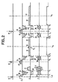
- figure 2 : des diagrammes temporels de signaux radiofréquence d'excitation, de signaux de champ magnétique perturbateur, et de signaux relevés dans une mesure particulière comportant une imagerie de type 2DFT d'une coupe d'un corps sous examen ;
- figures 3a et 3b : des diagrammes temporels de déphasages résultant, après application de séquences de champs magnétiques perturbateurs, entre les contributions émises par des particules fixes et des particules en mouvement ;
- figure 4 : une représentation schématique de la réponse d'une partie d'un milieu dont les particules sont en déplacement selon que ce déplacement est parallèle ou perpendiculaire à un plan de coupe ima- g^é.

The invention will be better understood on reading the description which follows and on examining the figures which accompany it. As mentioned above, this description and these drawings are given for information only and in no way limit the invention. In particular, the invention is only described in an imaging application. In the figures, the same references designate the same elements. They show:

- Figure 1: a machine for implementing the method according to the invention;
- Figure 2: time diagrams of excitation radiofrequency signals, disturbing magnetic field signals, and signals recorded in a particular measurement comprising 2DFT type imagery of a section of a body under examination;
- Figures 3a and 3b: time diagrams of phase shifts resulting, after application of disturbing magnetic field sequences, between the contributions emitted by fixed particles and moving particles;
- Figure 4: a schematic representation of the response of part of a medium whose particles are moving depending on whether this movement is parallel or perpendicular to an imaged cutting plane ^.

La figure 1 représente une machine utilisable pour mettre en œuvre le procédé de l'invention. Elle comporte des moyens symbolisés par une bobine 1 pour soumettre un corps 2 à un champ magnétique important et constant Bo. Le champ Bo est le champ orientateur. La machine comporte encore des moyens générateurs 3 et bobines 4, reliés aux moyens générateurs 3, pour soumettre le corps ainsi placé à des séquences d'excitation radiofréquence en présence de séquences de champ perturbateur : des gradients de champ orientés selon trois axes de référence de la machine X, Y ou Z (figure 2). Les bobines 4 représentent en même temps les bobines radiofréquence et les bobines de gradient de champ. La machine comporte encore des moyens de réception 5, reliés aux bobines 4, pour recevoir le signal de résonance magnétique. Dans une application d'imagerie, des moyens 6 peuvent permettre de calculer et de mémoriser une première image l₁ et une deuxième image 1₂ d'une coupe 7 du corps 2. Les deux images sont relatives à deux séries d'expérimentation imposées par des commandes symbolisées C₁ et C₂ des moyens générateurs 3. Dans des moyens de comparaison 8 on compare point à point les images l₁, 1₂, et on élabore une troisième image Is. On peut visualiser cette image 1₃ sur un dispositif de visualisation 50.FIG. 1 shows a machine which can be used to implement the method of the invention. It comprises means symbolized by a coil 1 for subjecting a body 2 to a large and constant magnetic field Bo. The Bo field is the orienting field. The machine also includes generator means 3 and coils 4, connected to the generator means 3, for subjecting the body thus placed to radio frequency excitation sequences in the presence of disturbing field sequences: field gradients oriented along three reference axes of machine X, Y or Z (Figure 2). The coils 4 represent the radio frequency coils and the field gradient coils at the same time. The machine also includes receiving means 5, connected to the coils 4, for receiving the magnetic resonance signal. In an imaging application, means 6 can make it possible to calculate and store a first image l ₁ and a second image 1 ₂ of a section 7 of the body 2. The two images relate to two series of experiments imposed by commands symbolized C ₁ and C ₂ of the generating means 3. In comparison means 8, the images l ₁ , 1 ₂ are compared point to point, and a third image Is is produced. This image 1 ₃ can be viewed on a device display 50.

Dans les images 1₁, 1₂, ou 1₃, un point d'image, ou pixel p, représente classiquement par sa luminosité la densité de particules contenue dans un élément de volume, ou voxel v qui lui correspond dans la tranche 7. Le voxel v comporte de nombreuses particules animées de vitesses V comportant des composantes V_x, Vy et V_z sur chacun des trois axes de référence de la machine. L'invention va permettre de calculer dans le voxel v, et pour tous les autres voxels aussi, la vitesse moyenne et le nombre des particules de ce voxel ainsi en mouvement. L'image 1₃ est représentative de cette information de vitesse, par comparaison entre deux images Il et 1₂ où l'effet de cette vitesse aura été modulée de deux manières différentes.In the images 1 ₁ , 1 ₂ , or 1 ₃ , an image point, or pixel p, conventionally represents by its brightness the density of particles contained in an element of volume, or voxel v which corresponds to it in section 7. The voxel v comprises numerous animated particles of velocities V comprising components V _x , Vy and V _z on each of the three reference axes of the machine. The invention will make it possible to calculate in the voxel v, and for all the other voxels also, the average speed and the number of the particles of this voxel thus in motion. Image 1 ₃ is representative of this speed information, by comparison between two images II and 1 ₂ where the effect of this speed will have been modulated in two different ways.

Dans un premier temps, on va rappeler brièvement la théorie de l'imagerie par une méthode de type 2DFT. Dans cette méthode comme dans toutes les autres il existe des gradients perturbateurs. Dans un deuxième temps on va rappeler pourquoi cette méthode est préférée eu égard à des problèmes d'inhomogénéité du champ orientateur. Dans un troisième temps, on indiquera, dans cet exemple, comment se calculent les champs compensateurs nécessaires pour moduler l'effet de la vitesse.First, we will briefly recall the theory of imagery using a 2DFT type method. In this method as in all the others there are disturbing gradients. In a second step we will recall why this method is preferred in view of problems of inhomogeneity of the orienting field. In a third step, we will indicate, in this example, how the compensating fields necessary to modulate the effect of speed are calculated.

Pour localiser une région d'un milieu il est nécessaire de repérer la nature de son émission en fonction de conditions locales de champ magnétique. Ces conditions locales sont imposées de façon à ce que la fréquence et la phase d'émission soient bien caractéristiques de la localisation dans l'espace de cette région du milieu. Pour cela on superpose au champ principal B_o des gradients de champ magnétique pulsés. Ces gradients sont orientés selon des directions X, Y, Z pour définir à tout moment les éléments de volume qui résonnent à des fréquences connues. Pour l'acquisition d'une image entière les conditions locales sont imposées en des séquences programmées (C₁, C₂). Celles-ci sont mises en mémoire dans un ordinateur pilote. Ces séquences définissent les instants d'application des gradients, les instants d'excitation des particules par les impulsions du champ radiofréquence, ainsi que les instants de lecture ou d'acquisition des données de l'image.To locate a region of a medium it is necessary to locate the nature of its emission as a function of local magnetic field conditions. These local conditions are imposed so that the frequency and the phase of emission are well characteristic of the localization in space of this region of the medium. For this, superimposed on the main field B _o are pulsed magnetic field gradients. These gradients are oriented in directions X, Y, Z to define at any time the volume elements which resonate at known frequencies. For the acquisition of a whole image the local conditions are imposed in programmed sequences (C ₁ , C ₂ ). These are stored in a pilot computer. These sequences define the instants of application of the gradients, the instants of excitation of the particles by the pulses of the radiofrequency field, as well as the instants of reading or acquisition of the data of the image.

La méthode d'imagerie 2DFT permet actuellement d'obtenir la meilleure qualité d'image. Dans cette méthode d'imagerie seul un plan de coupe, le plan 7 est, excité à la fois. La figure 2 montre à cet effet des impulsions radiofréquence 10, 11 et 12 appliquées en présence d'un gradient de champ dit de sélection, par exemple orienté selon l'axe Z, et représenté respectivement par des impulsions 13, 14 et 15. Quand le gradient de sélection est orienté selon l'axe Z la coupe est transverse, c'est-à-dire selon un plan X, Y. Dans l'imagerie 2 DFT on code en phase les différents signaux acquis. Ceci est obtenu par une impulsion d'intensité variable d'un gradient dit déphaseur, d'axe perpendiculaire à un gradient dit de lecture, dont la direction est constante. Par exemple, pour une coupe transverse, le gradient de lecture peut être sur l'axe X et le gradient de déphasage peut être sur l'axe Y. Sur la figure 2, le gradient X est coté 16, le gradient Y est coté 17. Par une double transformée de Fourier spatiale l'image est reconstruite, d'où le nom de la méthode. Une amélioration de cette méthode peut d'ailleurs permettre d'obtenir simultanément des images de plusieurs coupes parallèles.The 2DFT imaging method currently provides the best image quality. In this imaging method only one section plane, plane 7 is, excited at a time. FIG. 2 shows for this purpose radio frequency pulses 10, 11 and 12 applied in the presence of a so-called selection field gradient, for example oriented along the Z axis, and represented respectively by pulses 13, 14 and 15. When the selection gradient is oriented along the Z axis the section is transverse, that is to say along an X, Y plane. In 2 DFT imagery, the different acquired signals are phase coded. This is obtained by a variable intensity pulse of a so-called phase shifter gradient, with an axis perpendicular to a so-called reading gradient, the direction of which is constant. For example, for a cross section, the reading gradient can be on the X axis and the phase shift gradient can be on the Y axis. In Figure 2, the X gradient is rated 16, the Y gradient is rated 17 By a double spatial Fourier transform the image is reconstructed, hence the name of the method. An improvement of this method can moreover make it possible to obtain images of several parallel sections simultaneously.

L'existence du précodage 17, qui prend un certain temps, repousse dans le temps la mesure du signal émis par le corps. Comme ce signal s'atténue très vite, on a imaginé d'en mesurer un écho. Cet écho est produit, au moment de l'application des impulsions radiofréquence 11 puis 12 par une réflexion de la dispersion de phase des contributions apportées par chacune des particules. Pour cette raison ces impulsions sont dessinées sur la figure 2 plus hautes que l'impulsion 10 puisqu'elles font basculer l'orientation des moments magnétiques des spins des particules de 180_° alors que l'impulsion 10 ne les avait fait basculer que de 90_°. Pour imager une coupe d'un corps il y a lieu de réaliser des séquences d'excitation d'écho de spin en présence de séquences de gradients de champ en un nombre aussi important de fois que la résolution de l'image attendue doit être plus précise. A chaque séquence d'excitation, le gradient déphaseur Y varie par pas succes- sⁱfs partant d'une certaine valeur jusqu'à la même valeur mais de signe opposé. Cette valeur dépend de la forme et de la durée du gradient 16 de lecture. Ce gradient déphaseur permet de faire tourner chaque moment magnétique de spin d'une phase variable, dépendant de son ordonnée suivant l'axe Y et de la valeur de ce gradient. Pour chaque image l₁ et 1₂ le gradient Y peut prendre successivement le même nombre de valeurs : d'une manière préférée la définition des deux images sera la même.The existence of precoding 17, which takes some time, postpones the measurement of the signal emitted by the body. As this signal fades very quickly, we imagined to measure an echo. This echo is produced, at the time of the application of the radiofrequency pulses 11 then 12 by a reflection of the phase dispersion of the contributions made by each of the particles. For this reason these pulses are drawn in FIG. 2 higher than the pulse 10 since they cause the orientation of the magnetic moments of the spins of the particles to be tilted by 180 _° whereas the pulse 10 had only tilted them by 90 _° . To image a section of a body, it is necessary to carry out sequences of excitation of spin echo in the presence of sequences of field gradients in as large a number of times as the resolution of the expected image must be more precise. At each excitation sequence, the phase shifter Y gradient varies stepwise succession s ⁱ fs starting from a certain value to the same value but of opposite sign. This value depends on the shape and the duration of the reading gradient 16. This phase shift gradient makes it possible to rotate each magnetic spin moment of a variable phase, depending on its ordinate along the Y axis and on the value of this gradient. For each image l ₁ and 1 ₂ the gradient Y can successively take the same number of values: in a preferred manner the definition of the two images will be the same.

Pour éviter un précodage parasite imposé par la fin 18 de l'impulsion 13, pour la partie de cette impulsion existant après la fin de l'impulsion radiofréquence 10, et par le début 19 de l'impulsion 16 de lecture il est connu d'appliquer sur ces axes respectivement des impulsions 20 et 21. L'intégrale temporelle de ces impulsions est la même mais de signe opposé, elles neutralisent l'effet parasite de codage. L'intégrale est entendue au sens d'intégrale dans le temps. Les surfaces hachurées 20 et 19 sont donc égales aux surfaces en pointillés 18 et 21 respectivement. Les impulsions 20 et 21 n'interfèrent pas dans la sélection de coupe puisqu'au moment où elles sont appliquées l'impulsion 10 n'est plus présente. Les impulsions 14 et 15 sont auto- neutralisées puisqu'elles comportent des portions respectivement 22 et 23, et 24 et 25 antisymétriques par rapport au milieu de l'impulsion radiofréquence, 11 et 12 pour lesquelles elles resélection- nent la coupe 7 dans le corps 2.To avoid a parasitic precoding imposed by the end 18 of the pulse 13, for the part of this pulse existing after the end of the radiofrequency pulse 10, and by the beginning 19 of the read pulse 16 it is known to apply pulses 20 and 21 to these axes respectively. The time integral of these pulses is the same but of opposite sign, they neutralize the parasitic coding effect. The integral is understood in the sense of integral in time. The hatched areas 20 and 19 are therefore equal to the dashed areas 18 and 21 respectively. The pulses 20 and 21 do not interfere in the cut selection since at the time when they are applied the pulse 10 is no longer present. The pulses 14 and 15 are self-neutralized since they comprise portions 22 and 23 respectively, and 24 and 25 which are antisymmetrical with respect to the middle of the radiofrequency pulse, 11 and 12 for which they reselect the section 7 in the body. 2.

La méthode d'imagerie de type 2 DFT est la plus utilisée dans la pratique du fait de sa rapidité d'acquisition (comparée à des méthodes 3D) et à sa robustesse vis-à-vis des imperfections du système physique, en particulier vis-à-vis des inhomogénéités du champ orientateur. Ceci s'apprécie particulièrement en comparaison avec des méthodes par rétroprojection ou avec des méthodes n'utilisant pas d'écho de spin. Cette méthode est en contrepartie la plus intrinsèquement sensible au déplacement des particules. L'immunité aux inhomogénéités du champ Bo de la méthode 2 DFT provient du fait que contrairement aux méthodes par rétroprojection le gradient codeur en fréquence est de même direction (le gradient de lecture X) et de même amplitude, G_L, d'une séquence à l'autre. L'inhomogénéité du champ Bo ne fait alors que déformer les lignes isofréquen- ces de résonance. Pendant la lecture du signal, l'in- homogénéité du champ devient l'équivalent d'une mauvaise linéarité du gradient de lecture. Les images sont en conséquence distordues mais sans la création de flou et sans la perte de résolution associées que l'on rencontre avec les méthodes par rétroprojection. Dans celles-ci en effet le gradient de lecture change d'orientation à chaque séquence et de ce fait il répartit les inhomogénéités du champ orientateur dans toute l'image pour laquelle il crée ainsi un flou.The type 2 DFT imaging method is the most used in practice because of its speed of acquisition (compared to 3D methods) and its robustness against imperfections of the physical system, in particular vis- vis-à-vis the inhomogeneities of the orienting field. This is particularly appreciated in comparison with rear projection methods or with methods not using spin echo. In return, this method is the most intrinsically sensitive to the movement of particles. The immunity to inhomogeneities of the Bo field of the 2 DFT method stems from the fact that, unlike rear projection methods, the frequency encoder gradient is in the same direction (the reading gradient X) and of the same amplitude, G _L , of a sequence to the other. The inhomogeneity of the Bo field then only distorts the isofrequency lines of resonance. During the reading of the signal, the inhomogeneity of the field becomes the equivalent of a bad linearity of the reading gradient. The images are consequently distorted but without the creation of blurring and without the associated loss of resolution which one meets with the methods by rear projection. In these indeed the reading gradient changes orientation with each sequence and therefore it distributes the inhomogeneities of the orienting field throughout the image for which it thus creates a blur.

Les figures 3a et 3b montrent le déphasage Δφ résultant dans la contribution de signal émis par deux particules d'un même voxel soumises à des perturbations identiques, quand l'une des particules (trait plein) est immobile alors que l'autre particule (tirets) est animée d'une vitesse V. La figure 3a montre le diagramme temporel d'un signal radiofréquence RF comportant une impulsion 26 pour créer un écho de spin. Selon un axe A un gradient de champ magnétique a été imposé en prenant avant et après l'impulsion 26, par exemple, une valeur G pendant une durée e à chaque fois. En un lieu donné to une particule préalablement excitée, immobile, vibre à une fréquence fo au début de l'application de l'impulsion 27. Pendant la durée e de cette impulsion 27 elle vibre à une fréquence différente. Par exemple cette fréquence est supérieure, de telle manière qu'à la fin de l'impulsion 27 on puisse considérer, puisqu'elle se remet à vibrer à la fréquence fo qu'elle a subi un déphasage φ1. Lors de l'application de l'impulsion radiofréquence 26 on peut admettre que tout se passe comme si la phase du signal émis par cette particule s'inversait : -₀₁. Pendant l'impulsion 28 qui a exactement la même alluré que l'impulsion 27 le phénomène de déphasage continue : la contribution se déphase encore de φ1. Mais ce dernier déphasage vient effacer l'effet du premier après qu'il ait été inversé par l'impulsion 26. En conséquence, la particule immobile en Io retrouve à la fin de l'impulsion 28 la phase qu'elle avait au début de l'impulsion 27. Il est utile de remarquer que le déphasage « est proportionnel d'une part à l'amplitude du gradient G et d'autre part à la durée pendant laquelle chaque impulsion du gradient est imposée. Plus généralement φ1 est proportionnel à l'intégrale de ce gradient pendant la durée d'existence de son impulsion si cette impulsion n'est pas exactement carrée.Figures 3a and 3b show the phase shift Δφ resulting in the contribution of the signal emitted by two particles of the same voxel subjected to identical disturbances, when one of the particles (solid line) is stationary while the other particle (dashes) ) is driven by a speed V. FIG. 3a shows the time diagram of an RF radio frequency signal comprising a pulse 26 to create a spin echo. According to an axis A a magnetic field gradient was imposed by taking before and after the pulse 26, for example, a value G for a duration e each time. In a given place to a previously excited, stationary particle, vibrates at a frequency fo at the start of the application of the pulse 27. During the duration e of this pulse 27 it vibrates at a different frequency. For example, this frequency is higher, so that at the end of the pulse 27 it can be considered, since it resumes vibrating at the frequency fo that it has undergone a phase shift φ1. During the application of the radio frequency pulse 26, it can be assumed that everything happens as if the phase of the signal emitted by this particle were reversed: - ₀₁ . During impulse 28 which has exactly the same shape as impulse 27 the phase shift phenomenon continues: the contribution is still dephased by φ1. But this latter phase shift erases the effect of the first after it has been inverted by pulse 26. Consequently, the motionless particle in Io finds at the end of pulse 28 the phase it had at the start of the pulse 27. It is useful to note that the phase shift "is proportional on the one hand to the amplitude of the gradient G and on the other hand to the duration during which each pulse of the gradient is imposed. More generally φ1 is proportional to the integral of this gradient during the duration of existence of its pulse if this pulse is not exactly square.

Il en va tout autrement pour une deuxième particule, toute voisine dans le même voxel de la particule précédente, et qui par contre est animée d'une vitesse V. Sur la figure 3a, on a indiqué que cette particule se trouvait successivement dans les positions 1₀ à 1₄ au début et à la fin de la première impulsion 27, au moment de l'impulsion radiofréquence 26, et au début et à la fin de la deuxième impulsion 28 du gradient. Après la première impulsion 27 de gradient, le déphasage résultant φ2 est proportionnel au gradient G et à la durée e. Mais il est aussi proportionnel à la distance l₁ - to parcourue dans l'intervalle par la particule. Cette distance est égale à V. e . Ce qui fait que le temps intervient maintenant au carré : la première portion de déphasage à l'allure d'une parabole (V.G.e²). De la fin de l'impulsion 27 au début de l'impulsion 28, tout se passe comme pour la particule immobile : la contribution possède une phase -φ2 au début de l'impulsion 28. Au cours de cette impulsion 28 l'évolution de la phase est également parabolique comme pour l'impulsion 27. On pourrait s'attendre à ce que les effets de phase s'effacent ici également. Cependant entre la fin de l'impulsion 27 et le début de l'impulsion 28 la particule animée s'est déplacée de la position 1₁ à la position l₃. Dans la position 1₃ au moment où l'impulsion 28 apparaît, et du fait de l'existence du gradient de champ, les conditions locales de champ ne sont plus les mêmes que celles qui avaient prévalu quand la particule s'était trouvée entre to et l₁. En conséquence à la fin de l'impulsion 28 la compensation ne s'opère pas et cette particule animée émet alors un signal déphasé d'une valeur Δφ que l'on peut écrire de la manière suivante :

où y est le rapport gyromagnétique des particules considérées, où G (e) représente le gradient dans les impulsions 27 et 28, et où T est la durée qui sépare l'apparition de ces deux impulsions. Si e n'est pas petit, T mesure la durée entre les milieux de ces impulsions. Plus généralement on peut écrire :

où le déphasage est donné maintenant en fonction du temps et où G (_T) représente toutes les perturbations appliquées aux particules avant qu'on en mesure à une date le signal qu'elles émettent. On se souvient simplement que les perturbations considérées sont telles que :

Car c'est sous cette condition que, d'une manière connue dans l'état de la technique (figure 2 impulsions 18 à 25), on a compensé les précodages parasites. On ne l'avait bien entendu pas fait pour l'impulsion variable 17 puisque le déphasage qu'elle provoque pour le signal global est, d'une acquisition à l'autre, une des caractéristiques permettant l'imagerie.It is quite different for a second particle, very close in the same voxel of the preceding particle, and which on the other hand is animated by a speed V. On figure 3a, it was indicated that this particle was successively in the positions 1 ₀ to 1 ₄ at the beginning and at the end of the first pulse 27, at the time of the radio frequency pulse 26, and at the start and at the end of the second pulse 28 of the gradient. After the first gradient pulse 27, the resulting phase shift φ2 is proportional to the gradient G and to the duration e. But it is also proportional to the distance l ₁ - to traveled in the interval by the particle. This distance is equal to V. e. This means that time now intervenes squared: the first portion of phase shift at the pace of a parabola (VGe ² ). From the end of pulse 27 to the start of pulse 28, everything happens as for the motionless particle: the contribution has a -φ2 phase at the start of pulse 28. During this pulse 28 the evolution of the phase is also parabolic as for impulse 27. One would expect that the phase effects will also disappear here. However between the end of pulse 27 and the start of pulse 28 the animated particle moved from position 1 ₁ to position l ₃ . In the position 1 ₃ at the moment when the impulse 28 appears, and due to the existence of the field gradient, the local field conditions are no longer the same as those which had prevailed when the particle was between and l ₁ . Consequently at the end of the pulse 28 the compensation does not take place and this animated particle then emits a phase shifted signal with a value Δφ which can be written in the following manner:

where y is the gyromagnetic ratio of the particles considered, where G (e) represents the gradient in

pulses

27 and 28, and where T is the duration which separates the appearance of these two pulses. If e is not small, T measures the duration between the midpoints of these pulses. More generally we can write:

where the phase shift is given now as a function of time and where G ( _T ) represents all the disturbances applied to the particles before we measure at a date the signal they emit. We simply remember that the disturbances considered are such that:

Because it is under this condition that, in a manner known in the state of the art (FIG. 2 pulses 18 to 25), the parasitic precodings have been compensated for. It was obviously not done for the variable pulse 17 since the phase shift it causes for the global signal is, from one acquisition to another, one of the characteristics allowing imaging.

En l'absence d'une impulsion radiofréquence telle que 26 créant un écho de spin (figure 3b), les impulsions 27 et 28 du gradient bipolaire doivent être remplacées par des impulsions 29, 30 de signes opposés. De cette manière la phase pour les particules fixes évolue jusqu'à φ3 en fin de l'impulsion 29 et évolue en sens inverse jusqu'à zéro au cours de l'impulsion inverse 30. Le déphasage Δφ entre la contribution des particules mobiles et celles des particules fixes est du même ordre que précédemment.In the absence of a radiofrequency pulse such as 26 creating a spin echo (FIG. 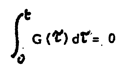3b), the pulses 27 and 28 of the bipolar gradient must be replaced by pulses 29, 30 of opposite signs. In this way the phase for the fixed particles evolves to φ3 at the end of the pulse 29 and evolves in opposite direction to zero during the inverse pulse 30. The phase shift Δφ between the contribution of the moving particles and those fixed particles is of the same order as before.

Dans l'expression de Δφ(t), G (r) représente donc toutes les séquences nécessitées par la mesure. Ce qui caractérise l'invention c'est que ces séquences sont maintenues telles quelles mais que leurs effets sur la vitesse sont compensés par l'adjonction de séquences supplémentaires de gradients de champ G' dits compensateurs tels que

où G' représente des gradients, eux aussi bipolaires, c'est-à-dire tels que

Autrement dit, en agissant ainsi on annule le coefficient multiplicateur de la vitesse V qui apparaît dans le calcul de Δφ(t). Du coup, quelle que soit cette vitesse, Δφ(t) est nul : toutes les contributions sont en phase. Les particules mobiles sont prises en compte comme si elles étaient fixes.In the expression of Δφ (t), G (r) therefore represents all the sequences required by the measurement. What characterizes the invention is that these sequences are maintained as they are but that their effects on the speed are compensated for by the addition of additional sequences of field gradients G 'called compensators such as

where G 'represents gradients, also bipolar, i.e. such that

In other words, by doing so we cancel the speed multiplier coefficient V which appears in the calculation of Δφ (t). Suddenly, whatever this speed, Δφ (t) is zero: all the contributions are in phase. Moving particles are taken into account as if they were fixed.

En revenant à la figure 2 on voit sur chaque axe X, Y, Z l'adjonction de tels gradients bipolaires compensateurs sous la forme préférée de couples d'impulsions notés 31 et 32, 33 et 34, 35 et 36, 37 et 38, 39 et 40 et 42 et 43. L'incidence de ces impulsions compensatrices est symbolisée dans le dessin par la présence de petites croix. On sait, dans les machines de l'état de la technique imposer de telles impulsions en modifiant les commandes C₁ ou C₂ des moyens générateurs. L'intégrale dans le temps des impulsions de chaque couple est nulle. D'une manière préférée, puisque l'impulsion de correction de précodage 20 sur l'axe de sélection Z est appliquée entre des dates t₁ et t₂ à la fin de l'impulsion 13, on applique l'impulsion 31 pendant la même période. Dans ce cas l'impulsion 20 "nouvelle" est plus forte. Les impulsions 35 et 37 sont également appliquées pendant cette période. Les impulsions 32, 36 et 38 d'une manière préférée sont appliquées entre la fin t₃ de l'impulsion 14 et le début t₄ de l'impulsion de lecture 16. Les impulsions 33, 39 et 42 sont appliquées entre la fin ts de l'impulsion 16 et le début t₆ de l'impulsion 15. Les impulsions 34, 40 et 43 sont appliquées entre la fin t₇ de l'impulsion 15 et le début t₈ d'une impulsion 41 qui sert à la lecture d'un deuxième écho.Returning to FIG. 2, we see on each axis X, Y, Z the addition of such compensating bipolar gradients in the preferred form of pairs of pulses denoted 31 and 32, 33 and 34, 35 and 36, 37 and 38, 39 and 40 and 42 and 43. The incidence of these compensating impulses is symbolized in the drawing by the presence of small crosses. It is known, in the machines of the state of the art, to impose such pulses by modifying the commands C ₁ or C ₂ of the generating means. The time integral of the pulses of each couple is zero. Preferably, since the precoding correction pulse 20 on the selection axis Z is applied between dates t ₁ and t ₂ at the end of the pulse 13, the pulse 31 is applied during the same period. In this case the "new" pulse 20 is stronger. The pulses 35 and 37 are also applied during this period. The pulses 32, 36 and 38 are preferably applied between the end t ₃ of the pulse 14 and the start t ₄ of the read pulse 16. The pulses 33, 39 and 42 are applied between the end ts of pulse 16 and the start t ₆ of pulse 15. Pulses 34, 40 and 43 are applied between the end t ₇ of pulse 15 and the start t ₈ of pulse 41 which is used for reading a second echo.

Sur le plan pratique, la mesure du signal émis est effectuée entre des dates t'4 et t's contenues entre les dates t₄ et t₅ et aussi pendant la durée de l'impulsion 41. Bien entendu les impulsions de compensation appliquées sur un axe, X, Y ou Z ont pour objet d'effacer l'effet des gradients perturbateurs appliqués sur le même axe. L'expression intégrale donne implicitement les gradients G' ; il est possible de faire des simplifications. Premièrement tous les termes en G (τ).τ sont des termes connus (ils appartiennent à la séquence 2DF^T) : leur intégrale l'est également. Cette intégrale peut donc être sortie de l'expression. D'une manière préférée les formes des impulsions compensatrices 31 à 43 seront des formes connues et, dans la mesure du possible, identiques à des formes déjà pratiquées pour les impulsions normales des séquences perturbatrices. Compte tenu des dates retenues pour l'application de ces impulsions, une intégrale unitaire de chacune d'elle peut être calculée et l'expression de G' peut s'écrire d'une autre manière :

Le premier membre est connu il concerne les gradients perturbateurs. Le deuxième membre comporte des intégrales de gradients de forme préférée r et d'amplitude unité. On sait calculer l'intégrale du deuxième membre puisqu'on connaît la forme choisie r. En conséquence on peut en déduire 1 c'est-à-dire l'amplitude des impulsions compensatrices.On a practical level, the measurement of the signal emitted is carried out between dates t'4 and t's contained between dates t ₄ and t ₅ and also during the duration of pulse 41. Of course the compensation pulses applied on an axis , X, Y or Z are intended to erase the effect of the disturbing gradients applied on the same axis. The integral expression implicitly gives the gradients G '; it is possible to make simplifications. Firstly all the terms in G (τ) .τ are known terms (they belong to the 2DF ^T sequence): their integral is also. This integral can therefore be taken out of expression. In a preferred manner, the shapes of the compensating pulses 31 to 43 will be known shapes and, as far as possible, identical to shapes already practiced for the normal pulses of the disturbing sequences. Given the dates chosen for the application of these pulses, a unit integral of each of them can be calculated and the expression of G 'can be written in another way:

The first member is known, it concerns disturbing gradients. The second member has integrals of gradients of preferred shape r and of unit amplitude. We know how to calculate the integral of the second member since we know the chosen form r. Consequently, we can deduce 1, that is to say the amplitude of the compensating pulses.

Dans le cas de l'imagerie conventionnelle, où un gradient au moins est appliqué pendant la période de lecture (t'₄, 1'₅), l'équation implicite contenant G' ne peut être vérifiée pour tout 1. Mais on doit au moins la vérifier aux temps t_Ei, t_E2... centre des phases de mesure. Ces dates sont celles où l'écho de spin attendu est le plus fort. Elles sont telles que la durée séparant la date de l'impulsion radiofréquence 10 et t_E, est le double de la durée entre l'impulsion 10 et l'impulsion 11, et telles que la durée entre la date t_E1 et la date t_E2 est égale au double de la durée entre la durée tE₁ et la date de l'impulsion radiofréquence 12.... La justification de ces dates est, d'une part, intuitive et, d'autre part, théorique. L'idée conductrice en ce domaine est que l'on cherche à connaître l'état de la coupe 7 non pas au moment de son excitation (impulsion 10) mais au moment, tE₁ ou t_E2 où justement on effectue la mesure : au centre du signal émis.In the case of conventional imagery, where at least one gradient is applied during the reading period (t ' ₄ , 1' ₅ ), the implicit equation containing G 'cannot be verified for all 1. But we must at less check it at times t _Ei , t _{E2 ...} center of the measurement phases. These dates are those when the expected spin echo is strongest. They are such that the duration separating the date of the radiofrequency pulse 10 and t _E , is twice the duration between the pulse 10 and the pulse 11, and such that the duration between the date t _E1 and the date t _E2 is equal to twice the duration between the duration tE ₁ and the date of the radiofrequency pulse 12 .... The justification of these dates is, on the one hand, intuitive and, on the other hand, theoretical. The guiding idea in this area is that we seek to know the state of the section 7 not at the time of its excitation (pulse 10) but at the time, tE ₁ or t _E2 where precisely the measurement is carried out: center of the transmitted signal.

Tous les termes de l'équation implicite donnant G' étant connus, G' est calculable. Sur la figure 2 on va donner une approche simple de ce calcul. Pour l'axe X on sait que les impulsions 21 et 19 situées de part et d'autre de l'impulsion radiofréquence 11 neutralisent mutuellement leurs effets de précodage : l'intégrale de la somme de ces impulsions est nulle. Par contre l'intégrale du produit de ces impulsions par la durée qui les sépare de la date du relevé, t_Ei, n'est pas nulle : l'impulsion 21 étant plus antérieure dans le temps que l'impulsion 19. Tout se passe donc comme si l'impulsion 21 de "force" donnée est appliquée à un "bras de levier" plus long que l'impulsion 19 de force égale. L'effet sur la phase de l'impulsion 19 est bien entendu inverse de celui de l'impulsion 21 puisqu'elles sont situées de part et d'autre de l'impulsion 11. En conséquence leur effet commun sur la phase s'analyse comme un moment orienté dans le sens de l'impulsion ayant le plus grand bras de levier : l'impulsion 21. Il convient de contrecarrer ce moment résultant par un couple d'impulsions 35, 36 dont l'intégrale totale est nulle (il ne provoque aucun déphasage sur le signal des parties fixes) mais dont le moment global s'oppose au moment global des deux impulsions 21 et 19. Ainsi, l'impulsion 35 étant placée dans le temps à une date plus antérieure que l'impulsion 36 par rapport à la date t_E1 son effet est prépondérant. Il est bien de sens opposé à l'impulsion 21.All the terms of the implicit equation giving G 'being known, G' is calculable. In Figure 2 we will give a simple approach to this calculation. For the X axis, it is known that the pulses 21 and 19 located on either side of the radiofrequency pulse 11 mutually neutralize their precoding effects: the integral of the sum of these pulses is zero. On the other hand, the integral of the product of these impulses by the duration which separates them from the date of the reading, t _Ei , is not zero: the impulse 21 being more anterior in time than the impulse 19. Everything happens therefore as if the pulse 21 of given "force" is applied to a "lever arm" longer than the pulse 19 of equal force. The effect on the phase of the pulse 19 is of course opposite to that of the pulse 21 since they are located on either side of the pulse 11. Consequently their common effect on the phase is analyzed as a moment oriented in the direction of the pulse having the largest lever arm: pulse 21. It is necessary to counteract this moment resulting in a couple of pulses 35, 36 whose total integral is zero (it does not causes no phase shift on the signal of the fixed parts) but whose global moment is opposed to the global moment of the two pulses 21 and 19. Thus, the pulse 35 being placed in time on a date earlier than the pulse 36 by compared to the date t _E1 its effect is preponderant. It is of opposite direction to impulse 21.

De la même façon sur l'axe de sélection Z, des impulsions 18 et 20, et 22 et 23, ce sont à chaque fois les impulsions 18 et 22 qui priment : leur bras de levier est plus long. En conséquence on conçoit bien que l'impulsion 31 doit être dans le même sens que l'impulsion 20. Le cas des impulsions 37 et 38 est un peu différent. En effet elles doivent contrecarrer les effets d'un gradient qui varie d'une acquisition à l'autre. Les amplitudes des impulsions 37 et 38 varieront donc également en correspondance d'une acquisition à l'autre (symbolisé par des flèches). Pour les raisons précédentes quand l'impulsion 17 est positive l'impulsion 37 doit être négative. Pour pouvoir réduire les amplitudes des impulsions compensatrices on cherche bien entendu à donner à leur moment le plus d'efficacité possible : on essaie d'augmenter la durée qui sépare leur application de la date du relevé. On les place le plus en amont possible de la séquence pour la première (31, 35, 37) et le plus en aval pour la deuxième (32, 36, 38). En conclusion elles sont le plus éloignées possible de part et d'autre de l'impulsion radiofréquence 11 ; et elles sont le plus éloignées possible l'une de l'autre.In the same way on the selection axis Z, pulses 18 and 20, and 22 and 23, it is each time the pulses 18 and 22 which take precedence: their lever arm is longer. Consequently, it will be appreciated that the pulse 31 must be in the same direction as the pulse 20. The case of the pulses 37 and 38 is a little different. In fact, they must counteract the effects of a gradient which varies from one acquisition to another. The amplitudes of the pulses 37 and 38 will therefore also vary in correspondence from one acquisition to another (symbolized by arrows). For the above reasons when pulse 17 is positive pulse 37 must be negative. In order to be able to reduce the amplitudes of the compensating pulses, it is of course sought to give the most possible efficiency at their moment: we try to increase the duration which separates their application from the date of the reading. They are placed as far upstream as possible in the sequence for the first (31, 35, 37) and as far downstream for the second (32, 36, 38). In conclusion, they are as far apart as possible on either side of the radiofrequency pulse 11; and they are as far apart from each other as possible.

Lors du premier relevé, en t_Ei, les effets de vitesse des parties mobiles ont été complètement compensés. On compense maintenant au moyen des impulsions 33 et 34 les effets de la deuxième impulsion de sélection 15. La date pivot pour le calcul des moments est maintenant la date t_E2. Sur l'axe de lecture X on compense également par deux impulsions 42 et 43 les effets de la deuxième moitié 60 de l'impulsion 16 et de la première moitié 61 de l'impulsion 41. La présence des impulsions compensatrices 39 et 40 sur l'axe Y se justifie par le fait que l'impulsion 17 n'est pas bipolaire. Car la compensation de son moment à la date pivot t_E1 par les impulsions 37 et 38 n'implique pas une telle compensation à une autre date pivot telle que ts₂. Et ceci bien qu'aucune impulsion supplémentaire de perturbation n'intervienne sur cet axe entre-temps.During the first survey, at t _Ei , the speed effects of the moving parts were completely compensated. We now compensate by means of pulses 33 and 34 for the effects of the second selection pulse 15. The pivotal date for calculating the moments is now the date t _E2 . On the reading axis X, the effects of the second half 60 of the pulse 16 and of the first half 61 of the pulse 41 are also compensated by two pulses 42 and 43. The presence of the compensating pulses 39 and 40 on the Y axis is justified by the fact that the pulse 17 is not bipolar. Because the compensation of its moment on the pivotal date t _E1 by pulses 37 and 38 does not imply such compensation on another pivotal date such as ts ₂ . And this although no additional disturbance pulse intervenes on this axis in the meantime.

La figure 4 représente un tube d'écoulement 51 sensé se trouver dans la tranche examinée 7 du corps 2. Le haut de la figure représente une situation dans laquelle l'axe du tube 51 est situé dans le plan X, Y de la coupe. Dans la partie basse de la figure la situation est différente : le tube 51 est supposé être perpendiculaire au plan X et Y de la coupe. De part et d'autre sont représentés des voxels notés 52 à 55. Ces voxels ont la forme de parallélépipèdes rectangles ayant une forme de section sensiblement carrée. La section est carrée dans la mesure où, dans l'imagerie, l'échantillonnage représentatif est effectué avec la même résolution selon l'axe X et l'axe Y du plan de coupe. La grande longueur du parallélépipède rectangle s'étend selon l'axe Z. Cette longueur est liée à l'épaisseur de la coupe 7. Cette épaisseur est un compromis expérimental entre la finesse de résolution des coupes et la quantité de signal global mesurable. Plus la coupe est épaisse plus le signal mesurable est élevé, et bien entendu moins l'image est précise. Dans la pratique la grande dimension est de l'ordre de 7 à 15 mm, la section carrée est de l'ordre de 1 mm par 1 mm.FIG. 4 represents a flow tube 51 supposed to be in the examined section 7 of the body 2. The top of the figure represents a situation in which the axis of the tube 51 is located in the plane X, Y of the section. In the lower part of the figure the situation is different: the tube 51 is assumed to be perpendicular to the plane X and Y of the section. On both sides are represented voxels denoted 52 to 55. These voxels have the shape of rectangular parallelepipeds having a shape of substantially square section. The section is square insofar as, in the imagery, the representative sampling is carried out with the same resolution along the X axis and the Y axis of the section plane. The great length of the rectangular parallelepiped extends along the axis Z. This length is linked to the thickness of the section 7. This thickness is an experimental compromise between the fineness of resolution of the sections and the quantity of overall measurable signal. The thicker the cut, the higher the measurable signal, and of course the less precise the image. In practice, the large dimension is of the order of 7 to 15 mm, the square section is of the order of 1 mm by 1 mm.

Dans le conduit 51 un fluide non représenté circule avec un diagramme de vitesse 56. Les vitesses 57 des particules situées au centre sont plus élevées que les vitesses 58 des particules situées sur les bords du conduit. Dans les artères la vitesse 57 peut être de l'ordre de 50 cm par seconde. Les voxels 52 et 53 comportent, quand ils sont situés à l'aplomb de la section 59 du conduit 51, nécessairement des particules animées avec des vitesses très différentes. Avant l'invention l'étalement du spectre de vitesse était tellement important que la contribution des voxels 52 et 53 dans le signal global était nulle : on avait l'impression que le tube était creux. L'image des voxels 54 et 55 pouvait dans certains cas être révélatrice. Elle l'était dans la mesure où ces voxels se situaient à l'aplomb de la partie de la section du conduit où l'étalement du spectre des vitesses était faible. C'est le cas pour le voxel 55 où les vitesses (au centre du tube) tout en étant élevées sont relativement homogènes entre elles. Leur déphasage correspondant est sensiblement le même: la moyenne n'est pas nulle. Par contre pour le voxel 54 situé à l'aplomb du bord du conduit 51, là où l'évolution des vitesses est brutale, le signal restitué est nul. Il en résultait que l'image des tubes 51 perpendiculaires au plan de coupe était appréciée géométriquement plus petite qu'elle n'était en réalité. Avec l'invention l'image des écoulements est révélée fidèlement.In the duct 51 a fluid not shown circulates with a speed diagram 56. The speeds 57 of the particles located in the center are higher than the speeds 58 of the particles located on the edges of the duct. In the arteries the speed 57 can be of the order of 50 cm per second. The voxels 52 and 53 comprise, when they are located directly above the section 59 of the conduit 51, necessarily animated particles with very different speeds. Before the invention, the spreading of the speed spectrum was so important that the contribution of voxels 52 and 53 in the overall signal was zero: one had the impression that the tube was hollow. The image of voxels 54 and 55 could in some cases be revealing. It was so insofar as these voxels were located directly above the part of the section of the duct where the spread of the velocity spectrum was low. This is the case for the voxel 55 where the speeds (in the center of the tube) while being high are relatively homogeneous between them. Their corresponding phase shift is substantially the same: the average is not zero. On the other hand, for the voxel 54 located directly above the edge of the conduit 51, where the speed evolution is abrupt, the signal restored is zero. As a result, the image of the tubes 51 perpendicular to the cutting plane was appreciated geometrically smaller than it actually was. With the invention the image of flows is faithfully revealed.

On peut moduler l'effet de la vitesse avec le procédé de l'invention. Il suffit de ne pas annuler totalement le coefficient multiplicateur de V dans l'expression de a¢(i) où les gradients compensateurs sont présents. Dans l'invention on propose de réaliser une deuxième expérimentation dans laquelle la compensation n'est plus complète et dans laquelle en définitive la mesure est sensible à cet effet de vitesse. On compare ultérieurement les résultats obtenus au cours de ces deux expérimentations. On en déduit les caractéristiques de vitesse recherchées. D'une manière préférée on fera varier la modulation selon un axe particulier. Cet axe particulier peut être l'axe X, l'axe Y, l'axe Z, ou même un axe différent. Pour faire varier cette modulation on modifie l'amplitude (1) des impulsions de compensation appliquées respectivement sur les axes X, Y, Z ou sur une combinaison de ces axes.The effect of speed can be modulated with the method of the invention. It suffices not to completely cancel the multiplying coefficient of V in the expression of a ¢ (i) where the compensating gradients are present. In the invention, it is proposed to carry out a second experiment in which the compensation is no longer complete and in which, ultimately, the measurement is sensitive to this speed effect. The results obtained during these two experiments are subsequently compared. We deduce the desired speed characteristics. In a preferred manner, the modulation will be varied according to a particular axis. This particular axis can be the X axis, the Y axis, the Z axis, or even a different axis. To vary this modulation, the amplitude (1) of the compensation pulses applied to the X, Y, Z axes or to a combination of these axes is modified.

Dans la deuxième expérimentation on s'arrange pour que la sensibilité à l'effet de vitesse soit telle que, pour la vitesse nominale attendue à mesurer, l'écart maximal de phase soit de l'ordre de ou inférieur à un radian. Dans ces conditions on peut montrer que l'information de vitesse est obtenue simplement en calculant le rapport de la variation relative des mesures, d'une expérience à l'autre, à la mesure de la première (ou de la deuxième) expérience. Autrement dit si S1 est le résultat de la première expérience, et si S2 est le résultat de la deuxième, l'information de vitesse moyenne est représenté par (Si - S₂)/Si. Au-delà de cette sensibilité d'une part le calcul proposé n'est plus applicable tel quel pour connaître l'information de vitesse, et d'autre part la sensibilité risque d'être tellement forte qu'on retomberait dans les difficultés que l'invention a résolues. C'est un calcul de ce type qu'effectuent les moyens de comparaison 8. Le calcul est entrepris pixel par pixel. D'une expérimentation à l'autre la sensibilité est passée de zéro à une certaine valeur calculable par l'intégrale de G (_T)._T et de G' (r ).τ. On peut donc quantifier la vitesse mesurée.In the second experiment, arrangements are made so that the sensitivity to the speed effect is such that, for the nominal speed expected to be measured, the maximum phase difference is of the order of or less than a radian. Under these conditions it can be shown that the speed information is obtained simply by calculating the ratio of the relative variation of the measurements, from one experiment to another, to the measurement of the first (or second) experiment. In other words if S1 is the result of the first experiment, and if S2 is the result of the second, the average speed information is represented by (Si - S ₂ ) / Si. Beyond this sensitivity on the one hand the proposed calculation is no longer applicable as is to know the speed information, and on the other hand the sensitivity may be so strong that we would fall back into difficulties that the invention has resolved. It is a calculation of this type that is carried out by the comparison means 8. The calculation is undertaken pixel by pixel. From one experiment to another, the sensitivity went from zero to a certain value that can be calculated by the integral of G ( _T ). _T and G '(r) .τ. We can therefore quantify the measured speed.

Dans une variante préférée l'invention est mise en oeuvre dans une méthode d'excitation avec écho de gradient. Cette méthode est préférée à une méthode avec écho de spin comme décrit jusqu'ici. En effet dans une méthode avec écho de spin, l'impulsion radiofréquence qui fait basculer de 180_° les moments magnétiques des particules a une bande en fréquence légèrement surévaluée, redondante (de durée plus courte), pour bien rephaser les contributions de toutes les particules qui étaient entrées en résonance à cause de l'impulsion à 90_°. Cette redondance peut provoquer en elle-même l'excitation parasite de particules voisines de la tranche 7. Or maintenant avec la compensation, ces particules voisines peuvent être codées (par l'impulsion 38 ou 40). Donc le signal parasite qu'elles produisent peut varier d'une séquence à l'autre. Dans ces conditions, on ne sait plus l'extraire du signal utile. S'il reste constant en effet, en faisant une double acquisition, on peut le supprimer. S'il n'est pas supprimé sa présence peut être gênante.In a preferred variant, the invention is implemented in an excitation method with gradient echo. This method is preferred to a method with spin echo as described so far. Indeed in a method with spin echo, the radiofrequency pulse which makes the magnetic moments of the particles switch 180 _° has a slightly overvalued, redundant frequency band (of shorter duration), to properly rephasize the contributions of all the particles which had come into resonance because of the 90 _° pulse. This redundancy can in itself cause parasitic excitation of neighboring particles of wafer 7. Now, now with compensation, these neighboring particles can be coded (by pulse 38 or 40). So the spurious signal they produce can vary from one sequence to another. Under these conditions, we no longer know how to extract it from the useful signal. If it remains constant indeed, by making a double acquisition, it can be deleted. If it is not removed, its presence can be troublesome.

Dans une séquence avec écho de gradient (figure 2) l'impulsion radiofréquence 11 (et 12...) est supprimée. L'impulsion 14 de deuxième sélection n'a plus lieu d'exister. L'impulsion 21 d'équilibrage de l'impulsion de lecture 16 est de sens opposé. L'impulsion 17 est inchangée. L'écho de gradient est provoqué par l'égalité des aires 21 (inversée) et 19. Dans ces conditions les gradients perturbateurs ont tous des allures comparables à ceux de la figure 3b. On les compense néanmoins selon le même principe que pour ceux de la figure 3a. Pour la compensation du gradient de codage de phase les impulsions de compensation 37 et 38 sont maintenues telles quelles. Comme il n'y a plus d'écho de spin il ne peut plus y avoir de signal parasite que l'on ne saurait pas éliminer.In a sequence with gradient echo (Figure 2) the radio frequency pulse 11 (and 12 ...) is suppressed. The second selection pulse 14 no longer exists. The pulse 21 for balancing the read pulse 16 is in the opposite direction. Pulse 17 is unchanged. The gradient echo is caused by the equality of the areas 21 (inverted) and 19. Under these conditions the disturbing gradients all have gaits comparable to those of FIG. 3b. They are nevertheless compensated according to the same principle as for those of FIG. 3a. For compensation of the phase coding gradient, the compensation pulses 37 and 38 are maintained as they are. As there is no longer any spin echo there can no longer be a parasitic signal which cannot be eliminated.

Claims

1 A method for the modulation of the effect of velocity of mobile parts of a body (2) during an operation measuring density by nuclear magnetic resonance, for which measuring operation

- the body (2) is submitted to a constant orientating magnetic field (Bo) in order to orientate magnetic spin moments of the body (2) in a single direction (Z),

- the body (2) is subjected to magnetic excitation due to a first radiofrequency pulse (10) in the presence of and/or followed by the application of a sequence of magnetic disturbing field (13, 14 and 17),

- a detecting a radiofrequency signal emitted by the body in response, in which method one modulates the effect of velocity (V) of mobile parts of the body created by the sequence of the disturbing field by the application, prior to detection (t_Ei), of a sequence (31 - 43) of pulses of a compensating magnetic field, whose integral with respect to duration is zero, and whose history and value are a function of the history and value of the disturbing field, the pulses of the compensating magnetic field being determined in form (r), in duration, and in position (t₁ - t2) and the amplitude (k) thereof being evaluated in order to obtain the desired modulation.

2 The method as claimed in claim 1 in accordance with which the sequence of the disturbing magnetic field comprises magnetic field pulses on three orthogonal axes (X, Y and Z) and the sequence of the compensating magnetic field comprises magnetic field pulses on these three same axes, in order to modulate one by one the effects of velocity of the mobile parts of the body on these same three axes.

3 The method as claimed in claim 1 or claim 2 in accordance with which the sequence of the magnetic compensating fields comprises bipolar pulse couples.

4 The method as claimed in any one of the preceding claims 1, 2 and 3, wherein the sequence of compensating magnetic fields comprises pulse couples, each pulse of a couple being in value, in form, in duration and in sign equal to the other pulse of the couple, such pulses respectively coming before and after a second radiofrequency pulse.

5 The method as claimed in any one of the preceding claims 1 through 4, in which the integral of the product of the value of the pulses of the disturbing field and the duration of time separating them from the detection of the signal emitted is compensated by the integral of the same product obtained with the pulses of the compensating field.

6 The method as claimed in claim 3 or claim 4, wherein the pulses of the pulse couples comprise pulses which are furthest apart from each other.

7 The method as claimed in any one of the preceding claims 1 through 6, wherein the radiofrequency magnetic excitation comprises a first radiofrequency pulse (10) in order to cause a 90_° swing of the orientation of the magnetic spin moments, followed by at least a second (11) radiofrequency magnetic pulse to cause a swing of 1800 of the magnetic moments of the spings, and in which one detects (t_E) as the magnetic resonance signal the echo of the signal emitted in response after it has been reflected by the second radiofrequency pulse (11).

8 The method as claimed in any one of the preceding claims 1 through 6, wherein the radiofrequency magnetic excitation comprises a first radiofrequency pulse (10) in order to cause a 90_° swing of the orientation of the magnetic spin moments, followed by a first echo gradient pulse (29) and one detects as a magnetic resonance signal the echo of the signal emitted in response after it has been reflected by a second gradient pulse (30).

9 The method as claimed in any one of the preceding claims 1 through 8, wherein the measuring operation comprises the production of the image of a volume whose position and whose dimensions are determined by the sequence (13 - 15) of the disturbing magnetic field.

10 The method as claimed in any one of the preceding claims 1 through 8, wherein the measuring operation comprises the production (6) of an image of a section of a section (7) of the body whose position within the body is determined by the sequence (13 - 15) of the disturbing magnetic field.

11 The method as claimed in claim 9, wherein the production of the image is performed using a method of the inverse Fourier transformation type with three dimensions (3DFT).

12 The method as claimed in claim 7, wherein the production of the image is performed using a method of inverse Fourier transformation type with two dimensions (2DFT).

13 The performance of the method as claimed in any one of the preceding claims 1 through 12, wherein said method is performed a first time (11) in order to compensate for the effect of velocity, and a second time (1₂) modifying one or more of the characteristics of the compensating magnetic field, and the readings are compared (8 and 1₃) which are obtained during such operations in order to deduce the velocity of the mobile pits concerned.

14 The performance of the method as claimed in claim 13, when same relates to the performance of the method in accordance with one of the claims 2 through 12, in accordance with which the modification relates to characteristics of the compensating magnetic field relative to one axis in order to deduce therefrom the velocity component of the mobile parts on this axis.

15 The performance of the method as claimed in claim 13 or in the claim 14, wherein the modification is such that the corresponding phase offset (△ϕ(t)) with respect to the signal emitted by the mobile parts moving at a nominal velocity is of the order of one radian.