DE60223253T2 - IMPROVED PROCESS CONTROL - Google Patents
IMPROVED PROCESS CONTROL Download PDFInfo
- Publication number
- DE60223253T2 DE60223253T2 DE60223253T DE60223253T DE60223253T2 DE 60223253 T2 DE60223253 T2 DE 60223253T2 DE 60223253 T DE60223253 T DE 60223253T DE 60223253 T DE60223253 T DE 60223253T DE 60223253 T2 DE60223253 T2 DE 60223253T2
- Authority
- DE
- Germany
- Prior art keywords
- control
- control solution
- controlled variable
- parameter
- solution
- Prior art date
- Legal status (The legal status is an assumption and is not a legal conclusion. Google has not performed a legal analysis and makes no representation as to the accuracy of the status listed.)
- Expired - Lifetime
Links
Classifications
-
- G—PHYSICS
- G05—CONTROLLING; REGULATING
- G05B—CONTROL OR REGULATING SYSTEMS IN GENERAL; FUNCTIONAL ELEMENTS OF SUCH SYSTEMS; MONITORING OR TESTING ARRANGEMENTS FOR SUCH SYSTEMS OR ELEMENTS
- G05B17/00—Systems involving the use of models or simulators of said systems
- G05B17/02—Systems involving the use of models or simulators of said systems electric
-
- G—PHYSICS
- G05—CONTROLLING; REGULATING
- G05B—CONTROL OR REGULATING SYSTEMS IN GENERAL; FUNCTIONAL ELEMENTS OF SUCH SYSTEMS; MONITORING OR TESTING ARRANGEMENTS FOR SUCH SYSTEMS OR ELEMENTS
- G05B13/00—Adaptive control systems, i.e. systems automatically adjusting themselves to have a performance which is optimum according to some preassigned criterion
- G05B13/02—Adaptive control systems, i.e. systems automatically adjusting themselves to have a performance which is optimum according to some preassigned criterion electric
- G05B13/04—Adaptive control systems, i.e. systems automatically adjusting themselves to have a performance which is optimum according to some preassigned criterion electric involving the use of models or simulators
- G05B13/048—Adaptive control systems, i.e. systems automatically adjusting themselves to have a performance which is optimum according to some preassigned criterion electric involving the use of models or simulators using a predictor
Abstract
Description
Die Erfindung betrifft eine verbesserte Prozesssteuerung, insbesondere eine verbesserte modellgestützte Prozesssteuerung.The The invention relates to an improved process control, in particular an improved model-based Process control.
Moderne automatisierte Prozesse, wie etwa Herstellungsprozesse, werden unter strengen und im Allgemeinen hochkomplexen Steuerungsregimen ausgeführt, sowohl um die Effizienz zu maximieren, als auch, um Fehler oder Betriebsversagen zu vermeiden. In ihrer einfachsten Form basieren diese Regime üblicherweise auf einem Rückkopplungssystem, durch das ein Parameter des Prozesses überwacht und als ein Steuerungsparameter zum Vergleich mit einem Zielwert an eine Steuerungseinrichtung übergeben wird, wobei der Zustand des Prozesses als eine Funktion des Steuerungsparameters verändert wird, um dem Zielwert zu folgen.modern Automated processes, such as manufacturing processes, are submerged both rigorous and generally highly complex control regimes to maximize efficiency, as well as errors or operational failure to avoid. In their simplest form, these regimes are usually based on a feedback system, by monitoring a parameter of the process and as a control parameter for comparison with a target value passed to a control device with the state of the process as a function of the control parameter changed will be to follow the target value.
Ein
bekanntes und etabliertes Steuerungsregime ist das der Modell-prädikativen
Regelung (MPC), das in "Model
Predictive Control; past, present and future." von Morari, M. & J. H. Lee (1999) Comput. Chem. Engng.
23, 667–682,
beschrieben ist. Das Grundprinzip ist in
Bezugnehmend
auf
Dieser
Vorgang wird online und in Echtzeit durchgeführt und ist in
Mathematisch
kann das Prozess- oder Anlagenmodell im Zustandsraum durch die Gleichungen
beschrieben werden:
Die Variable u repräsentiert die Regelgrößen oder die durch die Steuerungseinrichtung zur Steuerung des Prozesses manipulierten Prozesseingänge, x die Prozesszustände, d. h. Messwerte, die für die aktuellen Werte von einer oder mehreren Prozessgrößen repräsentativ sind und y die Messungen des Prozessausgangs. Bei Mehrvariablen-Prozessen sind x, y und u selbstverständlich Vektoren und A und B Matrizen. Die Ausgangs- und Regelgrößen sind begrenzt durch die Minimal- und Maximalwerte, welche Beschränkungen des Prozesses bilden.The Variable u represents the controlled variables or by the controller for controlling the process manipulated process inputs, x the process states, d. H. Measured values for the current values of one or more process variables representative and y are the measurements of the process output. For multi-variable processes, x, y and u of course Vectors and A and B matrices. The output and controlled variables are limited by the Minimum and maximum values, which form restrictions of the process.
Die Gleichungen stellen mathematisch dar, wie zu einem Zeitpunkt t in einem Prozess der zukünftige Zustand des Prozesses in einem diskreten, nachfolgenden Zeitintervall t + 1 abhängig von dem gemessenen Zustand x zum Zeitpunkt t und den zum Zeitpunkt t eingesetzten Regelgrößen vorhergesagt wird – diese Berechnung wird dann, immer noch zum Zeitpunkt t, auf der Grundlage der Berechnung für den Zeitpunkt t + 1 vorwärts iteriert für den vorhergesagten Zustand zum Zeitpunkt t + 2 und so fort. Zum Zeitpunkt t ist der Prozessausgang ferner ein direkte Funktion des momentanen Prozesszustands. Der Prozessausgang wird in Gleichung (2) berechnet, um zu gewährleisten, dass er die Ausgangsbeschränkungen nicht überschreitet.The equations represent mathematically how at a time t in a process the future state of the process is predicted in a discrete subsequent time interval t + 1 depending on the measured state x at time t and the control variables used at time t - this calculation becomes then, still at time t, based on the calculation for time t + 1, iterates forward for the predicted state at time t + 2 and so forth. At time t, the process output is also a direct function of the current process state. The process output is in Equation (2) is calculated to ensure that it does not exceed the output constraints.
Es
hat sich gezeigt, dass die Iteration bis zu einem Zeitpunkt t +
Ny in Form des nachstehenden zu optimierenden
Problems dargestellt werden kann (siehe beispielsweise die vorstehend
genannte Veröffentlichung
von Morari & Lee): 
Gleichung (3) ist die iterierte Erweiterung von Gleichung (1). Der erste Terminus auf der rechte Seite umfasst eine quadratische Funktion der vorhergesagten Zustandsvariablen zum Zeitpunkt t + Ny unter Verwendung des transponierten Vektors x' und der Konstantenmatrix P. Der zweite Terminus ist eine Summierung aller zwischenliegenden vorhergesagten Zustandsvariablen von Zeitpunkt t bis Zeitpunkt t + Ny–1, unter Verwendung des transponierten Vektors x' und der Konstantenmatrix Q und, über den gleichen Bereich und wieder in quadratischer Form mit der Konstantenmatrix R, der entsprechenden Regelgrößen u. In beiden Fällen wird jeder folgende Zustandswert Xt+k+1 aus dem vorhergehenden Zustandswert xt+k unter Verwendung von Gleichung 1 abgeleitet. Jeder Wert von Ut+k wird abgeleitet als eine Funktion des vorhergesagten Zustandswerts für diesen Zeitpunkt und der Verstärkungsmatrix K. Die Beschränkungen für y und u werden bis zu einem Zeitpunkt Nc überwacht. Auf diese Weise wird die Funktion J konstruiert.Equation (3) is the iterated extension of equation (1). The first term on the right comprises a quadratic function of the predicted state variable at time t + N y using the transposed vector x 'and the constant matrix P. The second term is a summation of all intermediate predicted state variables from time t to time t + N y-1 , using the transposed vector x 'and the constant matrix Q and, over the same range and again in quadratic form with the constant matrix R, the corresponding controlled variables u. In either case, each subsequent state value X t + k + 1 is derived from the previous state value x t + k using Equation 1. Each value of U t + k is derived as a function of the predicted state value for that instant and the gain matrix K. The constraints for y and u are monitored until time N c . In this way, the function J is constructed.
Die
linke Seite von Gleichung (3) erfordert, dass aus dem Lösungsraum
eine optimale Lösung
ausgewählt
wird, indem die Funktion J des Zustands x(t) und der Vektor U der
Regel-/Eingangsgrößen für alle Zeitintervalle
minimiert werden. Die Funktion J wird im Regelgrößenraum minimiert, das heißt, der
Optimalwert von U erfüllt
Gleichung (3) einschließlich
der verschiedenen Bedingungen im Feld "Unter Berücksichtigung von", so dass J minimal
wird. Die erhaltenen Werte von u(t) und x(t) sind dann wie in
Ein wesentliches Problem besteht bei der praktischen Ausführung von MPC, da die für die Berechnung in Echtzeit benötigte Verarbeitungsleistung sehr hoch ist. Wenn eine Vielzahl von Variablen erforderlich sind, wenn für komplexe Prozesse benötigte komplexe Steuerungsfunktionen oder äußerst kurze Zeitintervalle gewünscht sind, kann die Belastung sicherlich kosten-, energie-, oder sogar raumineffizient werden. Da die Lösung online erzeugt wird und nur auf momentane Bedingungen abgestimmt ist, stellt sie keine quantitativen Daten darüber zur Verfügung, ob das Modell selbst geeignet ist.One A major problem is the practical execution of MPC, since the for needed the calculation in real time Processing power is very high. If a lot of variables are required if for needed complex processes complex control functions or extremely short time intervals required The burden can certainly be cost, energy, or even become space inefficient. Because the solution generated online and matched only to current conditions is, it does not provide quantitative data on whether the model itself is suitable.
Verschiedene
Versuche, die Ausführung
von MPC zu verbessern, sind unternommen worden. In
Die vorliegende Erfindung ist in den unabhängigen Patentansprüchen angegeben. Einige fakultative Merkmale sind in den davon abhängigen Patentansprüchen angegeben.The The present invention is set forth in the independent claims. Some optional features are given in the dependent claims.
Gemäß der Erfindung wird ein Verfahren zur Ableitung einer expliziten Steuerungslösung für den Betrieb eines Systems bereitgestellt, wobei das System eine Regelgröße und einen messbaren Parameter hat, umfassend die Schritte des Offline-Konstruierens eines System-Betriebsmodells auf Basis dieser Regelgröße und des messbaren Parameters und des Offline-Konstruierens einer optimierten expliziten Steuerungslösung für diese Regelgröße und den messbaren Parameter unter Verwendung einer parametrischen Optimierung. Da die Lösung explizit und offline-konstruiert ist, kann die Online-Steuerung des Systems unter Verwendung der Lösung deutlich beschleunigt werden. Darüber hinaus kann die explizite Lösung offline überprüft werden, um Erkenntnisse über das Steuerungssystem/Steuerungsmodell selbst bereitzustellen.According to the invention becomes a method for deriving an explicit control solution for operation a system, wherein the system is a controlled variable and a has measurable parameters, including the steps of designing offline System operating model based on this controlled variable and the measurable parameter and constructing an optimized explicit control solution for them offline Controlled variable and the measurable parameters using parametric optimization. There the solution is explicit and offline-constructed, the online control of the system using the solution significantly accelerated become. About that In addition, the explicit solution be checked offline to Findings about to provide the control system / control model itself.
Die explizite Steuerungslösung ist vorzugsweise auf einer Datenspeichereinrichtung wie etwa einem Chip gespeichert und das System-Betriebsmodell ist vorzugsweise ein Modell-prädikatives Regelungs-("model predictive control", MPC)Modell. Die explizite Steuerungslösung ist vorzugsweise in der kontinuierlichen Zeit-Domäne konstruiert und ermöglich dadurch eine genauere Steuerung. Die MPC ist vorzugsweise als ein quadratisches Programm formuliert.The explicit control solution is preferably on a data storage device such as a chip and the system operating model is preferably a model predicative Regulatory ("model predictive control ", MPC) model. The explicit control solution is preferably constructed in the continuous time domain and enable thereby a more precise control. The MPC is preferably as a square one Program formulated.
Die Steuerungslösung umfasst vorzugsweise einen Koordinaten-Raum von mindestens einem Regelgrößen-Wertbereich, der einen Regelgrößen-Substitutionswert oder einen Regelgrößenwert als eine Funktion eines messbaren Parameterwerts aufweist, wobei die Koordinate der messbare Parameterwert ist. Dadurch wird ein einfaches und manipulierbares parametrisches Profil zur Verfügung gestellt. Der messbare Parameter kann einen messbaren Zustand oder eine Systemstörung umfassen. Das Verfahren kann ferner den Schritt des Analysierens der Steuerungslösung und des Konstruierens eines überarbeiteten System-Modells auf Basis dieser Analyse umfassen.The control solution preferably comprises a coordinate space of at least one The process variable value range, the one controlled variable substitution value or a controlled variable value as a function of a measurable parameter value, where the coordinate is the measurable parameter value. This will be a simple and manipulable parametric profile provided. The measurable parameter may include a measurable condition or a system failure. The method may further include the step of analyzing the control solution and of constructing a revised one System model based on this analysis include.
Gemäß der Erfindung wird darüber hinaus ein Verfahren zum Steuern des Betriebs eines Systems zur Verfügung gestellt, welches die Schritte des Online-Messens eines Parameters des Systems in einem ersten Zeitintervall, des Erhaltens einer Regelgröße auf Basis des gemessenen Parameters aus einer vor-definierten parametrisch optimierten expliziten Steuerungslösung und des Eingebens der Regelgröße in das System umfasst.According to the invention gets over it a method of controlling the operation of a system is provided, which the steps of online measurement of a parameter of the system in a first time interval, getting a controlled variable based of the measured parameter from a pre-defined parametric optimized explicit control solution and entering the Controlled variable in the System includes.
Die Schritte des Messens des Online-Zustands und des Ableitens der Regelgröße können in nachfolgenden Zeitintervallen wiederholt werden. Die Steuerungslösung umfasst vorzugsweise einen Koordinaten-Raum von mindestens einem Regelgrößen-Wertbereich mit einem Regelgrößen-Substitutionswert oder einer Regelgröße als Funktion eines gemessenen Zustandswerts, wobei die Koordinate der gemessene Zustandswert ist.The Steps of measuring the online state and deriving the controlled variable can be found in be repeated at subsequent time intervals. The control solution includes preferably a coordinate space of at least one controlled variable value range with a controlled variable substitution value or a controlled variable as a function a measured state value, wherein the coordinate of the measured State value is.
Gemäß der Erfindung wird darüber hinaus ein Steuerungssystem zum Steuern des Betriebs eines Systems zur Verfügung gestellt, das eine Regelgröße und einen messbaren Zustand hat, wobei das Steuerungssystem ein Systemzustands-Messelement, ein Datenspeicherelement, welches ein vor-definiertes parametrisch optimiertes explizites Steuerungslösungs-Profil speichert, einen Prozessor, der angeordnet ist, um eine Regelgröße von der Datenspeicherelement-Steuerungslösung auf der Basis eines gemessenen Systemzustands-Werts zu erhalten und eine Steuerungseinrichtung, die zum Eingeben der erhaltenen Regelgröße in das System angeordnet ist, inkludiert.According to the invention gets over it a control system for controlling the operation of a system to disposal which is a controlled variable and a measurable state, the control system being a system state measuring element, a data storage element which is a pre-defined parametric Optimized Explicit Control Solution Profile Saves One Processor arranged to set a controlled variable from the data storage element control solution get the basis of a measured system state value and a control device for entering the control variable received in the System is arranged, included.
Das Verfahren ist vorzugsweise in einem Computerprogramm implementiert, das in jedem beliebigen geeigneten computerlesbaren Medium gespeichert werden kann. Gemäß der Erfindung wird eine Datenspeichereinrichtung bereitgestellt, die eine durch ein Verfahren wie hier beschrieben abgeleitete Steuerungslösung speichert.The Method is preferably implemented in a computer program, stored in any suitable computer readable medium can be. According to the invention a data storage device is provided which includes a store a method as described herein derived control solution.
Ausführungsformen der Erfindung werden nachfolgend mit Bezugnahme auf die Zeichnungen beispielhaft beschrieben, wobei:embodiments The invention will be described below with reference to the drawings exemplified, wherein:
Die vorliegende Erfindung stellt eine alternative verbesserte Echtzeit-Lösung für die Probleme der modellgestützten Steuerung beispielsweise unter Verwendung der modellprädikativen Regelung zur Verfügung. Insbesondere durch Anwenden des allgemein als "parametrische Optimierung" bekannten Verfahrens auf das Prozessmodell, ermöglicht es die Erfindung, dass für alle vorkommenden Betriebsparameter Regelgrößen offline abgeleitet werden. Die auf diese Weise konstruierte explizite analytische Steuerungslösung ist als Funktion der Betriebsparameter in einen Chip oder einen Datenspeicher eingebettet, so dass das Prozessmodell nicht zu jedem Zeitintervall optimiert werden muss, wodurch die Verarbeitungslast erheblich verringert wird. Stattdessen sind die Regelgrößen als Funktion der Betriebsparameter und/oder in Form einer Nachschlagetabelle sofort verfügbar. Darüber hinaus ist die Lösung offline beobachtbar und bietet Informationen über das zu lösende Problem.The The present invention provides an alternative improved real-time solution to the problems the model-based Control, for example, using the model predictive Regulation available. Especially by applying the method commonly known as "parametric optimization" on the process model it is the invention that for all occurring operating parameters control variables are derived offline. The explicit analytical control solution constructed in this way is as a function of the operating parameters in a chip or a data memory embedded, so the process model is not at any time interval must be optimized, which significantly reduces the processing load becomes. Instead, the controlled variables are a function of the operating parameters and / or in the form of a lookup table immediately available. Furthermore is the solution observable offline and provides information about the problem to be solved.
Parametrische OptimierungParametric optimization
Die
Verfahren der parametrischen Optimierung oder der parametrischen
Programmierung sind dem Fachmann wohl bekannt und die Grundprinzipien
sind dargelegt in Gal, T. (1995) "Postoptimal Analyses, Parametic Programming
and Related Topics",
de Gruyter, New York and Dua, V. & E.N.
Pistikopoulos (1999) "Algorithms
for the Solution of Multiparametric Mixed-Integer Nonlinear Optimization
Problems", Ind.
Eng. Chem. Res. 38, 3976–3987,
welche aufgrund ihres Zitats als in diese Beschreibung einbezogen
gelten. Im Wesentlichen ist parametrische Optimierung ein mathematisches
Verfahren, durch das ein Problem zuerst als Optimierungsproblem
formuliert wird, eine Zielfunktion und Optimierungsvariablen als
Funktion von Parametern in dem Optimierungsproblem erhalten werden
und auch der Bereich im Parameterraum erhalten wird, in dem die Funktionen
gültig
sind. In der allgemeinsten Form kann das parametrische Optimierungsproblem
formuliert werden als: 
Diese allgemeinste Ausführung erfordert Minimierung von z, einer Funktion der Optimierungs- oder Regelgrößen x und y, um diese als Funktion von Parametern zu erhalten, die beispielsweise durch den Vektor θ repräsentierte messbare Zustände oder Systemstörungen sein können. Die verallgemeinerte Ausführung deckt Fälle, in denen die Regelgrößen stetige Wertevektoren x, oder binäre Wertevektoren y sind. Die Parameterwerte θ sind durch minimale und maximale Beschränkungen begrenzt. In dem unten erörterten Beispiel sind die Parameterwerte messbare Zustände.These most general execution requires minimization of z, a function of the optimization or control variables x and y, to obtain these as a function of parameters, for example represented by the vector θ measurable states or system errors could be. The generalized design covers Cases, in which the controlled variables are continuous Value vectors x, or binary Value vectors y are. The parameter values θ are by minimum and maximum restrictions limited. In the below discussed Example are the parameter values measurable states.
Lösungen für verschiedene
Sonderfälle
sind bekannt. Wo beispielsweise keine Regelgröße y (d. h. keine binäre Variable)
vorhanden ist, ist f(x) quadratisch und konvex in x, wo f(x) als
konvex definiert ist, wenn für jedes
x1, x2 ∈ X und
0 ≤ α ≤ 1, f[(1 – α)x1 + αx2] ≤ (1 – α)f(x1) + αf(x2) und g(x) linear in x ist, wird das Problem reduziert
auf das eines multiparametrischen quadratischen Programms (mp-QP).
Die Lösung
für diesen
Fall wird erörtert
in Dua et al. "An
algorithm for the solution of multi-parametric quadratic programs" (1999), tech. Rep.
D00.7, Centre for Process Systems engineering, Imperial College
London, welche aufgrund ihres Zitats als in diese Beschreibung einbezogen
gilt. Ein Beispiel für
die Form der Lösung
eines in Tabelle 1 angegebenen mp-QP-Problems wird nachfolgend erörtert. Tabelle
1 mp-OP-Beispiel:
Mathematische Formulierung 
Wie zu erkennen ist, ist die Funktion f(x) eine quadratische Funktion der Variablen x1, x2. Die Variablen x1 und x2 sind jeweils weiter beschränkt in Abhängigkeit von Zustandsparametern θ1, θ2, die wiederum begrenzt sind. Die Funktion wird im Raum der Regelgrößen x1, x2 minimiert, d. h. die Werte von x1, x2, für die f(x) optimiert ist, werden gefunden.As can be seen, the function f (x) is a quadratic function of the variables x 1 , x 2 . The variables x 1 and x 2 are each further limited in dependence on state parameters θ 1 , θ 2 , which in turn are limited. The function is minimized in the space of the controlled variables x 1 , x 2 , ie the values of x 1 , x 2 , for which f (x) is optimized, are found.
Die
nach der obenstehenden Verweisstelle (Dua et al.) erzeugte Lösung nimmt
die Form des in
Zulässiger Bereich 1permissible Area 1
- x1 = +0x1 = +0
- x2 = +0x2 = +0
- –1·t1 <= –0-1 · t1 <= -0
- +1·t1 <= +1+ 1 · t1 <= +1
- –1·t2 <= –0-1 · t2 <= -0
- +1·t1 + 1.18623·t2 <= +1.13188+ 1 * t1 + 1.18623 · t2 <= +1.13188
- –1·t1 + 1.80485·t2 <= +0.599143-1 · t1 + 1.80485 · t2 <= +0.599143
Zulässiger Bereich 2permissible Area 2
- x1 = +3.16515·t1 + 3.7546·t2 – 3.58257x1 = + 3.16515 · t1 + 3.7546 · t2 - 3.58257
- x2 = +1.8196·t1 – 3.2841·t2 + 1.0902x2 = + 1.8196 · t1 - 3.2841 · t2 + 1.0902
- +1·t2 <= +1+ 1 · t2 <= +1
- –1.38941·t1 – 1·t2 <= –1.19754-1.38941 · t1 - 1 · t2 <= -1.19754
- +1.34655·t1 – 1·t2 <= +0.0209892+ 1.34655 · t1 - 1 · t2 <= +0.0209892
Zulässiger Bereich 3permissible Area 3
- x1 = –0.584871·t1 + 1.0556·t2 – 0.350421x1 = -0.584871 · t1 + 1.0556 · t2 - 0.350421
- x2 = +1.819612 – 3.2841·t2 + 1.0902x2 = +1.819612 - 3.2841 · t2 + 1.0902
- –1·t1 <= –0-1 · t1 <= -0
- +1·t2 <= +1+ 1 · t2 <= +1
- +1.38941·t1 + 1·t2 <= +1.19754+ 1.38941 * t1 + 1 · t2 <= +1.17575
- +1·t1 – 1.80485·t2 <= –0.599143+ 1 · t1 - 1.80485 · t2 <= -0.599143
Zulässiger Bereich 4permissible Area 4
- x1 = +3.16515·t1 + 3.7546·t2 – 3.58257x 1 = + 3.16515 · t1 + 3.7546 · t2 - 3.58257
- x2 = –1.00203·t1 – 1.18864·t2 + 1.13418x 2 = -1.00203 · t1 - 1.18864 · t2 + 1.13418
- +1·t1 <= +1+ 1 · t1 <= +1
- +1·t2 <= +1+ 1 · t2 <= +1
- –1.3465511 + 1·t2 <= –0.0209892-1.3465511 + 1 · t2 <= -0.0209892
- –1·t1 – 1.18623·t2 <= –1.13188-1 · t1 - 1.18623 · t2 <= -1.13188
Es ist ersichtlich, dass für Bereich 1 x1 und x2 feste Werte haben, wohingegen für die Bereiche 2 bis 4 x1 und x2 als Funktionen der Koordinaten (θ1, θ2) ausgedrückt werden – man erkennt, dass x1 und x2 auf diese Weise innerhalb eines gegebenen Bereichs in Abhängigkeit von ihrer Position in diesem Bereich variieren werden.It can be seen that for region 1 x 1 and x 2 have fixed values, whereas for the regions 2 to 4 x 1 and x 2 are expressed as functions of the coordinates (θ 1 , θ 2 ) - it can be seen that x 1 and x 2 in this way will vary within a given range depending on their position in that range.
Ein weiterer Sonderfall liegt vor, wenn f(x) und g(x) linear in x sind. Das Problem wird dann als ein multi-parametrisches gemischt-ganzzahliges lineare Programm (engl.: multiparametric mixed-integer program, mp-MILP) dargestellt, für das Algorithmen entwickelt wurden, wie in Acevedo J. & Pistikopoulos E. N. "A Multiparametric Programming Approach for Linear Process Engineering Problems under Uncertainty" (1997) Ind. Eng. Chem. Res. 36, 717–728 erörtert, welche aufgrund ihres Zitats als in diese Beschreibung einbezogen gilt.One Another special case is when f (x) and g (x) are linear in x. The problem is then blended as a multi-parametric mixed-integer linear program (multiparametric mixed-integer program, mp-MILP) shown for the algorithms were developed, as in Acevedo J. & Pistikopoulos E.N. "A Multiparametric Programming Approach for Linear Process Engineering Problems under Uncertainty "(1997) Ind. Eng. Chem. Res. 36, 717-728 discussed, which are included as part of this description due to their quotation applies.
Ein mp-MILP Problem ist in Tabelle 2 angegeben.One mp-MILP problem is given in Table 2.
Tabelle 2Table 2
mp-MILP Beispiel: Mathematische Formulierungmp-MILP Example: Mathematical formulation
- z(θ) = min – 3x1 – 2x2 + 10y1 + 5y2 y, x s.t. x1 ≤ 10 + θ1 x2 ≤ 10 – θ1 x1 + x2 ≤ 20 x1 + 2x2 < 12 + θ1 – θ2 x1 – 20y1 ≤ 0 x2 – 20y2 ≤ 0 –x1 + x2 ≥ 4 – θ2 y1 + y2 ≥ 1 xn ≥ 0, n = 1, 2 yl ∈ {0, 1}, l = 1, 2 2 ≤ θs ≤ 5, s = 1, 2.z (θ) = min - 3x 1 - 2x 2 + 10y 1 + 5y 2 y, x st x 1 ≤ 10 + θ 1 x 2 ≤ 10 - θ 1 x 1 + x 2 ≤ 20 x 1 + 2x 2 <12 + θ 1 - θ 2 x 1 - 20y 1 ≤ 0 x 2 - 20y 2 ≤ 0 -x 1 + x 2 ≥ 4 - θ 2 y 1 + y 2 ≥ 1 x n ≥ 0, n = 1, 2 y l ∈ {0, 1}, l = 1, 2 2 ≤ θ s ≤ 5, s = 1, 2.
In
diesem Fall sind f(x) und g(x) lineare Funktionen der stetigen Variablen
x1, x2 und der binären Variablen
y1, y2. Die nach
der obenstehenden Verweisstelle (Acevedo & Pistikopoulos) erzeugte Lösung nimmt
die Form des in
Zulässiger Bereich 1permissible Area 1
- X1 = 0X 1 = 0
- x2 = 0.5·t1 – 0.5·t2 + 6x 2 = 0.5 · t1 - 0.5 · t2 + 6
- Binärer Vektor y = [0 1]binary Vector y = [0 1]
- –1·t1 <= –2-1 · t1 <= -2
- –1·t2 <= –2-1 · t2 <= -2
- +3·t1 – 1·t2 <= +8+ 3 · t1 - 1 · t2 <= +8
- +1·t2 <= +5+ 1 · t2 <= +5
Zulässiger Bereich 2permissible Area 2
- x1 = 0.333333·t1 + 0.333333·t2 + 1.333333x 1 = 0.333333 * t1 + 0.333333 * t2 + 1.333333
- x2 = 0.333333·1 – 0.666666·t2 + 5.333333x 2 = 0.333333 x 1 - 0.666666 x t2 + 5.333333
- Binärer Vektor y = [1 1]binary Vector y = [1 1]
- +1·t1 <= +5+ 1 · t1 <= +5
- –1·t2 <= –2-1 · t2 <= -2
- +2·t1 – 1·t2 <= +7+ 2 · t1 - 1 · t2 <= +7
- –11·t1 + 1·t2 <= –46-11 · t1 + 1 · t2 <= -46
- +1·t2 <= +5+ 1 · t2 <= +5
Zulässiger Bereich 3permissible Area 3
- x1 = 0x 1 = 0
- x2 = –1·t1 + 10x 2 = -1 · t1 + 10
- Binärer Vektor y = [0 1]binary Vector y = [0 1]
- –1·t2 <= –2-1 · t2 <= -2
- –3·t1 + 1·t2 <= –8-3 · t1 + 1 · t2 <= -8
- +11·t1 – 1·t2 <= +46+ 11 · t1 - 1 · t2 <= +46
- +1·t2 <= +5+ 1 · t2 <= +5
Zulässiger Bereich 4permissible Area 4
- x1 = –1·t1 + 1·t2 + 6x 1 = -1 · t1 + 1 · t2 + 6
- x2 = –1·t1 + 10x 2 = -1 · t1 + 10
- Binärer Vektor y = [1 1]binary Vector y = [1 1]
- +1·t1 <= +5+ 1 · t1 <= +5
- –1·t2 <= –2-1 · t2 <= -2
- –2·t1 + 1·t2 <= –7-2 · t1 + 1 · t2 <= -7
- +1·t1 – 1·t2 <= +2.66667+ 1 · t1 - 1 · t2 <= +2.66667
Zulässiger Bereich 5permissible Area 5
- x1 = 0x 1 = 0
- x2 = –1·t1 + 10x 2 = -1 · t1 + 10
- Binärer Vektor y = [0 1]binary Vector y = [0 1]
- +1·t1 <= +5+ 1 · t1 <= +5
- –1·t2 ≤ –2-1 · t2 ≤ -2
- 1·t1 + 1·t2 <= –2.66667 worin t1 und t2 θ1 bzw. θ2 entsprechen:1 · t1 + 1 · t2 <= -2.66667 where t1 and t2 correspond to θ 1 and θ 2, respectively:
Weiterhin dürfte ersichtlich sein, dass die Darstellung der Lösung in dieser einfachen, expliziten Form Erkenntnisse über das Steuerungsverfahren als Ganzes bietet. Insbesondere zeigt sie an, in welchem Maße die Zustandsmessungen zur Prozesssteuerung benötigt werden. Bei komplexeren Prozessen mit einer Vielzahl von gemessenen Zuständen ist es durchaus möglich, dass die explizite Lösung sich als unabhängig von einem oder mehreren der gemessenen Zuständen erweist, wodurch die Prozesssteuerungs-Hardware so ausgestaltet oder modifiziert werden kann, dass die entsprechende Zustandsmessungseinrichtung eliminiert wird und die Software so ausgestaltet oder modifiziert werden kann, dass die Verarbeitung betreffender Daten von gemessenen Zuständen eliminiert wird und so das Prozesssteuerungs-Schema für effizienten und kostengünstigen Betrieb auf allen Ebenen entsteht.Farther might be clear that the representation of the solution in this simple, explicit Form knowledge about the control process as a whole offers. In particular, she shows to what extent the State measurements for process control are needed. For more complex Processes with a variety of measured states, it is quite possible that the explicit solution to be independent of one or more of the measured states proving, thereby, the process control hardware can be designed or modified so that the corresponding Condition measuring device is eliminated and the software so can be designed or modified that processing of related data is eliminated from measured states and so on the process control scheme for efficient and cost effective Operation at all levels arises.
Dem Fachmann werden weitere Sonderfälle bewusst sein, für die die Lösung durch parametrische Optimierung bekannt ist und daher kann auf deren Erörterung an dieser Stelle verzichtet werden.the Become a specialist more special cases be aware of the solution is known by parametric optimization and therefore can be based on their discussion be waived at this point.
Anwendung von Verfahren der parametrischen OptimierungApplication of procedures of parametric optimization
Wenn
man sich dieser Verfahren bedient, kann ein modellgestütztes Problem
gemäß der vorliegenden Erfindung
optimiert werden unter Verwendung einer parametrischen Optimierung,
die Steueraktionen als eine Funktion von Messungen aus einer zu
steuernden Anlage bereitstellt, indem die Regelgrößen als
die Optimierungsvariablen und der Zustand der Anlage als Parameter
definiert werden. Im Echtzeitbetrieb wird diese Funktion dann, sobald
die Messungen von der Anlage bezogen wurden, ausgewertet, um unter
Verwendung der allgemein in
Nach
diesem Ansatz wird in bekannter Weise für die Anlage/das System/den
Prozess
Zurückkommend
auf das MPC-Problem der Gleichung (3), kann die Funktion J(U, x(t))
als ein Problem der quadratischen Programmierung (QP) formuliert
werden, indem man die in Gleichung (3) für xt+k+1,
zum Zeitpunkt t dargelegte Formel als die Summierung erweitert: ![]()
![]()
Dieser
Terminus wird in Gleichung (3) eingesetzt, um durch einfache algebraische
Manipulation das QP-Problem zu ergeben: ![]()
![]()
Das
durch Gleichung (6) dargestellte QP-Problem kann wieder unter Verwendung
einfacher algebraischer Manipulation als das mp-QP-Problem formuliert
werden:
worin z Δ U +
H–1F'x(t), z ∈ ![]()
where z ΔU + H -1 F'x (t), z ∈ ![]()
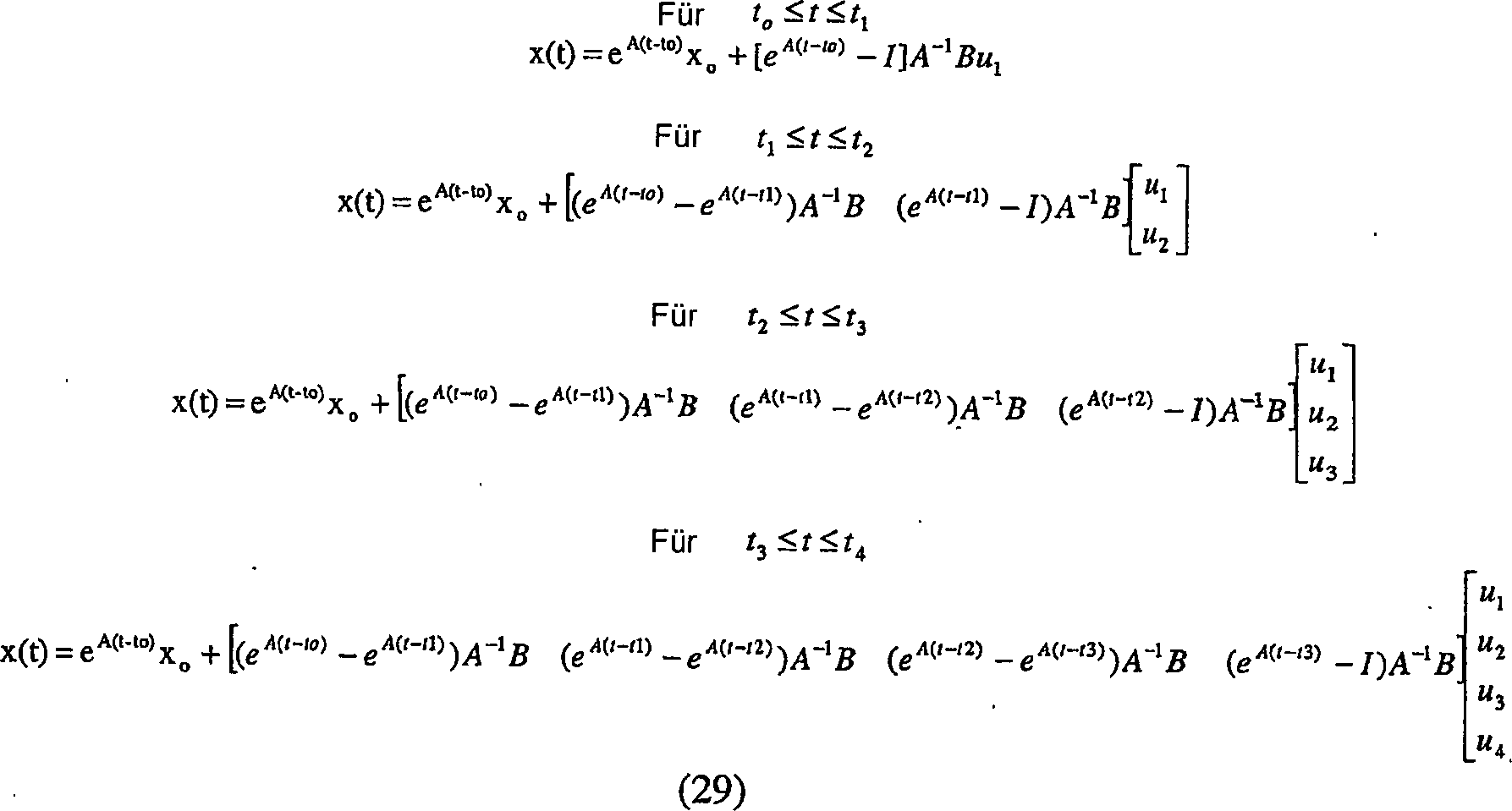
Es ist erkennbar, dass vorstehende Ableitung auf der Grundlage von Vorhersagen für diskrete zukünftige Intervalle t, t + 1 ... t + k durchgeführt wird, d. h. in der diskreten Zeit-Domäne, ähnliche Verfahren können jedoch eingesetzt werden, um das mp-QP-Problem in der kontinuierlichen Zeit-Domäne zu erhalten, d. h. Messungen werden weiter zu diskreten Intervallen t durchgeführt, aus diesen Messungen werden jedoch zukünftige kontinuierliche Profile der Zustandsgröße zu einem Zeitpunkt t + k vorhergesagt, wobei die zwischenliegenden Intervalle t + 1 ... t + k – 1 infinitesimal sind.It can be seen that the above derivation on the basis of Predictions for discrete future Intervals t, t + 1 ... t + k is performed, d. H. in the discreet Time domain, similar However, procedures can be used to the mp-QP problem in the continuous Time domain to obtain, d. H. Measurements will continue at discrete intervals t performed, however, these measurements will become future continuous profiles the state quantity to a Time t + k predicted, with intermediate intervals t + 1 ... t + k - 1 are infinitesimal.
In
diesem Fall wird Gleichung (6) neu geschrieben als: 
Anfangsbedingung
(I. C.).: x(to) = xo(θ, v)
B1·v(ti) + A1·x(ti) + C1·θ(ti) + b ≤ 0 
![]()
![]()
![]()
![]()
![]()
Initial condition (IC): x (t o ) = x o (θ, v)
B 1 · v (t i ) + A 1 · x (t i ) + C 1 · θ (t i ) + b ≤ 0 ![]()
![]()
![]()
![]()
![]()
Man beachte, dass in (8) in dem kontinuierlichen Modell Integrale und Differentialgleichungen vorliegen, wohingegen in (3) in der Zielfunktion und dem diskretisierten Modell Summierung vorlag. Problem (8) ist beschrieben in (i) Anderson, B.D. & J.B. Moore (1989) "Optimal Control: Linear Quadratic Methods", Prentice Hall, Englewood Cliffs, New Jersey, (ii) Bryson, A.E. & Y. Ho (1975) "Applied Optimal Control", Taylor and Francis, New York, und (iii) Kwakernak, H. & R. Sivan (1972) "Linear Optimal Control Systems", Wiley Interscience, New York, die alle aufgrund ihres Zitats als in diese Beschreibung einbezogen gelten.you notice that in (8) in the continuous model integrals and Differential equations exist, whereas in (3) in the target function and the discretized model summation. Problem (8) is described in (i) Anderson, B.D. & J.B. Moore (1989) "Optimal Control: Linear Quadratic Methods ", Prentice Hall, Englewood Cliffs, New Jersey, (ii) Bryson, A.E. & Y. Ho (1975) "Applied Optimal Control ", Taylor and Francis, New York, and (iii) Kwakernak, H. & R. Sivan (1972) "Linear Optimal Control Systems, "Wiley Interscience, New York, all because of their quote as in this Description included.
Das Ergebnis einer parametrischen Analyse von Problem (8) ist, das optimale Ziel (φ) und die Optimierungsvariablen (v) als Funktion der Parameter (θ) für den gesamten Raum der Parameterveränderungen auszudrücken. Dies kann dadurch erreicht werden, dass Problem (8) in eine Form transformiert wird, die mit den aktuellen Verfahren der parametrischen Programmierung des stabilen Zustands gelöst werden kann. Eine derartige Form ist in diesem Fall die mp-QP-Ausführung.The The result of a parametric analysis of problem (8) is the optimal one Target (φ) and the optimization variables (v) as a function of the parameters (θ) for the whole To express the space of the parameter changes. This can be achieved by transforming problem (8) into a form will be using the current method of parametric programming of the stable state solved can be. Such a shape in this case is the mp-QP design.
Durch
Anpassen der Parametrierung des Steuervektors, um das Problem der
optimalen Steuerung zu lösen
(e. g. "Off-line
Computation of Optimum Controls for Plate Distillation Column", Pollard & Sargent, 1970, Automatica
6, 59–76,
welche aufgrund ihres Zitats als in diese Beschreibung einbezogen
gilt), kann das Optimierungsproblem nur in dem reduzierten Raum
der Variablen v betrachtet werden. Dies erfordert selbstverständlich die
explizite Abbildung der Variablen x, die in den Beschränkungen
und dem Ziel als Funktionen von v und θ erscheinen. Diesen Ausdruck
kann man durch Lösen
des linearen ODE-Systems
in Gleichung (8) erhalten. Die Lösung
dieses Systems ist exakt und ist bei zeitinvarianten Parametern
und Optimierungsvariablen durch den analytischen Ausdruck gegeben: ![]()
![]()
Die
Integralauswertung in Gleichung (9) erfordert, dass die Form des
Profils der Ungewissheits- und Regelgrößen über die Zeit spezifiziert ist.
Regelgrößen sind üblicherweise
als stückweise
polynomische Funktionen über
die Zeit dargestellt, in denen die Werte der Koeffizienten im Polynom
während
der Optimierung festgelegt werden (Vassiliadis, V.S., R.W.H. Sargent & C.C. Pantelides
(1994) "Solution
of a Class of Multistage Dynamic Optimization Problems. 1. Problems
without Path Constraints." Ind.
Eng. Chem. Res. 33, 2111–2122,
welche aufgrund ihres Zitats als in diese Beschreibung einbezogen
gilt). Man beachte, dass, wenn die Ordnung des Polynoms als null
angenommen wird, die Steuerungsprofile einer stückweisen konstanten Diskretisierung
entsprechen. Was den Fall der Ungewissheit, θ, betrifft, ist dieser durch
Verwendung periodischer harmonischer Oszillationen, beschrieben,
d. h. Sinusfunktionen über
die Zeit mit ungewisser Amplitude oder ungewissem Mittelwert (Kookos,
I.K. & J.D. Perkins
(2000) "An Algorithm
for Simultaneous Process Design and Control", Tech. Rep. A019, Centre for Process
Systems Eng., Imperial College, London, welche aufgrund ihres Zitats
als in diese Beschreibung einbezogen gilt). Es ist zu bemerken,
dass komplexere Formen periodischer Funktionen durch Fourieranalyse
auf eine lineare Kombination von Sinusfunktionen reduziert werden
können.
Durch Einsetzen von (9) in (8) und damit durch Eliminieren des Systems
von Differentialgleichungen wird das Problem wie folgt transformiert: 
Indem man die Matrixzeitintegrale in Gleichung (10) auswertet, wird die Zielfunktion explizit als quadratische zeitinvariante Funktion nur der Parameter θ und der Regelgrößen v ausgedrückt. Dasselbe gilt jedoch nicht für die Wegbeschränkungen, die eine explizite Funktion der Regelgrößen, der Parameter und der Zeit sind. Die Zeitabhängigkeit solcher Beschränkungen macht Problem (10) unendlich-dimensional. Diese Schwierigkeit wird überwunden durch Anwenden der folgenden Methodik zur Konvertierung der unendlich-dimensionalen weg-zeit-varianten Beschränkungen in eine äquivalente endliche Anzahl von Punktbeschränkungen:
- 1. Gegeben sei eine begrenzte Anzahl von inneren Punktbeschränkungen, die nur an bestimmten Punkten innerhalb des Horizonts erfüllt werden müssen.
- 2. Lösung des Optimierungsproblems für diese bestimmte Menge innerer Beschränkungen.
- 3. Prüfung, ob dieselben Beschränkungen für jeden Zeitpunkt während des gesamten Zeithorizonts erfüllt sind.
- 4. Wenn einige der Beschränkungen an bestimmten Punkten tk verletzt werden, Vermehren dieser Punkte in Schritt 1 und Fortfahren, bis die Beschränkungen für den gesamten Zeithorizont erfüllt sind.
- 1. Given a limited number of inner point constraints that need only be met at certain points within the horizon.
- 2. Solution of the optimization problem for this particular set of inner constraints.
- 3. Check that the same restrictions are met at all times during the entire time horizon.
- 4. If some of the restrictions at certain points t k are violated, increase these points in step 1 and continue until the restrictions for the entire time horizon are met.
Diese Methodik transformiert die Wegbeschränkungen, die während des gesamten Zeithorizonts erfüllt sein müssen, in eine äquivalente Folge von Punktbeschränkungen, die nur zu bestimmten Zeitpunkten gelten und daher inhärent endlich sind.These Methodology transforms the path restrictions that occur during the entire time horizon fulfilled have to be in an equivalent Sequence of point restrictions, which apply only at certain times and therefore inherently finite are.
Demzufolge
wird die Zeit in den Wegbeschränkungen
von (10) durch eine geeignete Menge fester Zeitpunkte tk,
k = 1 ... K ersetzt. Folglich werden die Beschränkungen zu einer linearen Funktion
nur der Regelgrößen und
Parameter. Daher ist die äquivalente
mathematische Beschreibung von Problem (10) die folgende: 
Problem (11) ist nun ein multi-parametrisches quadratisches Programm (mp-QP) und seine Lösung stellt ähnlich wie im zeitdiskreten Fall die Regelgrößen als eine Funktion der Zustandsgrößen und ungewissen Parameter zur Verfügung.problem (11) is now a multi-parametric quadratic program (mp-QP) and his solution is similar In the discrete-time case, the controlled variables as a function of the state variables and uncertain parameters available.
Infolgedessen
können
bekannte Verfahren der parametrischen Optimierung für mp-QP-Probleme auf MPC
Probleme in der diskreten oder kontinuierlichen Zeit-Domäne angewendet
werden, um die vollständige Lösungsmenge
für z und
damit u als eine affine Funktion von x zu erhalten mit der Form:
Eine Beschränkung des oben beschrieben Systems liegt darin, dass es Modellungenauigkeiten und dauernd auftretende Störungen nicht berücksichtigt, außer in dem Umfang, in dem die Störungen als zusätzliche Parameter modelliert werden können. Dementsprechend können ungenaue Vorhersagen des Prozessverhaltens zu Unausführbarkeiten wie etwa nicht spezifikationsgerechter Herstellung, übermäßiger Entsorgung von Abfällen oder sogar gefährlichem Anlagenbetrieb führen. Nachfolgend werden zwei allgemeine Methoden zur Kompensation von Störungen erörtert.A restriction of the system described above is that there are model inaccuracies and constantly occurring disturbances not considered, except to the extent that the disturbances as additional Parameters can be modeled. Accordingly, you can inaccurate predictions of process behavior to impracticability such as unspecified manufacturing, excessive disposal of waste or even dangerous Perform plant operation. Below are two general methods of compensation disorders discussed.
In realen Prozessen kommt es üblicherweise zu Störungen aufgrund von Sensorfehlfunktion, beeinträchtigter Leistungsfähigkeit des Prozesses oder Systems durch Katalysatorfouling, Geräusch, menschliches Versagen oder Fehlhandlungen, Kosten- oder Modellungenauigkeiten unter anderen möglichen Faktoren. Diese Störungen können nicht immer gemessen werden und dementsprechend ist es erwünscht, derartige Störungen beim Ableiten des optimalen Steuerungsgesetzes zu berücksichtigen.In Real processes usually happen to disturbances due to sensor malfunction, degraded performance of the process or system by catalyst fouling, noise, human error or malfunctions, cost or model inaccuracies, among others potential Factors. These disorders can not always be measured and accordingly it is desirable to have such disorders to be taken into account when deriving the optimal control law.
Durch
Umschreiben der obigen Gleichung (3) erhält man eine passende Ausführung für das Ableiten eines
expliziten modellgestützten
Steuerungsgesetzes für
eine Prozessanlage wie folgt: 
![]()
![]()
![]()
![]()
![]()
![]()
Indem
die aktuellen Zustände
xt als Parameter betrachtet werden, wird
Problem (13) als ein multi-parametrisches quadratisches Programm
(mp-QP) der in (7) gegebenen Form umgeformt. Die Lösung dieses Problems
entspricht einem expliziten Steuerungsgesetz für das System, das die optimale
Steueraktion in Abhängigkeit
von den aktuellen Zuständen
ausdrückt.
Die mathematische Darstellung dieser parametrischen Steuerung, die
der in (12) gegebenen ähnelt,
ist wie folgt:
worin Nc die Anzahl von Bereichen
im Zustandsraum ist. Matrizen ac, CR1 c und Vektoren bc, CR2 c werden
aus der Lösung
des Problems der parametrischen Programmierung bestimmt und der
Index c kennzeichnet, dass jeder Bereich ein anderes Steuerungsgesetz
zulässt.
Vektor vct|0 ist das erste Element der Steuerungssequenz, ähnliche
Ausdrücke
werden für
die übrigen
Steuerungselemente abgeleitet.By considering the current states x t as a parameter, problem (13) is transformed into a multi-parametric quadratic program (mp-QP) of the form given in (7). The solution to this problem is an explicit control law for the system that expresses the optimal control action against the current states. The mathematical representation of this parametric control similar to that given in (12) is as follows:
where N c is the number of regions in the state space. Matrices a c , CR 1 c and vectors b c , CR 2 c are determined from the solution of the problem of parametric programming and the index c indicates that each domain allows a different control law. Vector v ct | 0 is the first element of the control sequence, similar expressions are derived for the rest of the control elements.
Die im vorhergehenden Absatz beschriebene modellgestützte parametrische Steuerung berücksichtigt nicht die Auswirkungen der persistenten langsam veränderlichen ungemessenen Störungen und Ungewissheiten des vorstehend erörterten Typs, die entweder als Eingänge in das System gelangen oder aus Modellierungsfehlern und zeitvarianten Prozesseigenschaften hervorgehen. Diese Störungen ergeben ein Offset, d. h. eine dauerhafte Abweichung der Ausgangvariablen von ihren Zielwerten und können zusätzlich Beschränkungsverletzungen verursachen. Wie nachstehend erörtert, werden gemäß der Erfindung zwei mögliche Lösungsverfahren eingeführt: Proportional Integral (P1) Steuerung und Nachregelung des Ursprungs. Die geeignete Nachregelung des Modells nach Störungs-Berechnungen ermöglicht die rekursive Online-Anpassung der modellgestützten Steuerung an die aktuellen Bedingungen.The model-based parametric control described in the preceding paragraph considered not the effects of persistent slow-changing unmeasured interference and uncertainties of the type discussed above, either as inputs get into the system or from modeling errors and time variations Process properties emerge. These disturbances give an offset, i. H. a permanent deviation of the output variables from their target values and can additionally restriction violations cause. As discussed below, be according to the invention two possible ones solution process introduced: Proportional Integral (P1) Control and readjustment of origin. The appropriate readjustment of the model after disturbance calculations allows the recursive online adaptation of the model-based control to the current ones Conditions.
In
der in
Der Grund für den Offset ist, dass das Modell das Vorhandensein der Störung nicht vorhergesagt hat.Of the reason for the offset is that the model does not know the presence of the fault predicted.
Dem ersten Ansatz gemäß der Erfindung folgend wird ein integraler Zustand in das modellgestützte Optimierungssystem einbezogen, um den Offset zu eliminieren. Dies stellt die offline abgeleitete parametrische proportionale integrale Steuerung ("Parametrischer PI") bereit. Wie untenstehend ausführlicher erörtert, wird insbesondere ein integraler Zustand in das dynamische System – und – mit einer bestimmten "Waiting Penalty" – auch in die Zielfunktion hinzugefügt. Das aktualisierte Problem wird erneut gelöst, um das oben erörterte modellgestützte parametrische Steuerungsgesetz zu erhalten.the first approach according to the invention Following is an integral state into the model-based optimization system included to eliminate the offset. This puts the offline derived parametric proportional integral control ("Parametric PI"). As below in more detail discussed, In particular, an integral state in the dynamic system - and - with a certain "Waiting Penalty "- also in added the objective function. The updated problem is again resolved to the model-based parametric To obtain control law.
Bei üblichen
Regelschemata, Seborg et al., (1989) "Process Dynamics & Control", Wiley & Sons, wird zur Dämpfung jeglicher dauerhaften
Abweichung der Ausgangvariablen von ihren Sollwerten durch das Vorhandensein
von Störungen
integrierendes Verhalten einbezogen. Dadurch entsteht die sogenannte
proportionale integrale Steuerung (PI-Steuerung). Hier wird die Einbeziehung
des integrierenden Verhaltens zum selben Zweck durch Einführung eines
integralen Zustands erreicht, der gleich der angenommenen Abweichungen des
Ausgangs von seinem Bezugspunkt, üblicherweise dem Ursprung,
ist. Dieser Zustand wird als eine zusätzliche quadratische Penalty
in der Zielfunktion erweitert (Kwakernaak & Sivan, 1972) "Linear Optimal Control Systems", John Wiley & Sons Ltd.. Dieses
Verfahren wurde ebenfalls durch das Generic Model Control-System
(Lee & Sullivan,
1988 "Generic Model
Control (GMC)" Comput.
Chem. Eng. 12(6), 573–580)
angenommen, aber in diesem Steuerungsschema werden keine Zustandsbeschränkungen
oder andere Modelleigenschaften berücksichtigt und für das Ableiten
der Steuerungsaktionen ist Online-Optimierung erforderlich. Nach Einbeziehung
des integralen Zustands wird Gleichung (13) wie folgt modifiziert: 
Gleichung (16) und die zugeordneten Bedingungen führen tatsächlich den zusätzlichen Zustand xq in die Zielfunktion ein als einen zusätzlichen Terminus und als eine zusätzliche Bedingung in Abhängigkeit von dem vorhergehenden integralen Zustandswert und dem jeweiligen Ausgang.equation (16) and the associated conditions actually carry the extra State xq in the objective function as an additional term and as one additional Condition in dependence from the previous integral state value and the respective one Output.
Durch
Eliminieren der dem dynamischen System zugeordneten Gleichheiten
und Betrachten der aktuellen reinen und integralen Zustände als
Parameter wird ein multiparametrisches quadratisches Programm, das
Gleichung (7) ähnlich
ist, formuliert. Die Lösung
dieses mp-QP entspricht dem folgenden stückweise affinen Steuerungsgesetz:
welches dem in Gleichung (12) gegebenen ähnlich ist.By eliminating the equations associated with the dynamic system and considering the actual pure and integral states as parameters, a multiparametric quadratic program similar to equation (7) is formulated. The solution of this mp-QP corresponds to the following piecewise affine control law:
which is similar to that given in equation (12).
Die durch Gleichung (4) beschriebene stückweise affine multivariable Steuerung enthält einen proportionalen Teil acxt(t*) bezogen auf die Zustände, einen integralen Teil dc xqt in Abhängigkeit von den Ausgängen und einen systematischen Fehler bc, demzufolge ist sie eine parametrische proportionale integrale Steuerung (parametrischer PI). Dieses Steuerungsgesetz ist asymptotisch stabil, dadurch garantiert es keinen Offset des stabilen Zustands von dem Zielpunkt unter der Bedingung, dass (i) die Dimension der Steuerungen größer ist oder gleich der Ausgangsdimension q ≥ m, was überwiegend bei Steuerungsproblemen der Fall ist (ii) die Open-Loop-Transfermatrix, die definiert ist von der Gleichung: H(s) = B1(sI – A1)–1A2 + B2 besitzt keine Nullen am Ursprung und (iii) die quadratische Kostenmatrix Q1, die den integralen Fehler penalisiert, ist positiv definit.The piecewise affine multivariable control described by Equation (4) includes a proportional part a c x t (t *) with respect to the states, an integral part d c xq t depending on the outputs, and a systematic error b c , hence it is a parametric proportional integral control (parametric PI). This control law is asymptotically stable, thereby guaranteeing no offset of the steady state from the target point under the condition that (i) the dimension of the controls is greater than or equal to the output dimension q ≥ m, which is predominantly in control problems (ii) Open loop transfer matrix defined by the equation: H (s) = B 1 (sI - A 1 ) -1 A 2 + B 2 has no zeros at the origin and (iii) the quadratic cost matrix Q 1 , which contains the penalized integral error, is positive definite.
Analog
kann differenzierendes Verhalten in das parametrische Steuerungsgesetz
aufgenommen werden. Eine algebraische Variable, die gleich der Differenz
zwischen der aktuellen und der vorhergehenden Ausgangsvariablen
ist, wird in den Ansatz eingeführt.
Diese Variable wird in der Zielfunktion wie folgt penalisiert: 
Die Lösung dieses Problems führt zu einer parametrischen Steuerung mit explizitem differenzierendem Verhalten, d. h. es resultiert ein parametrischer Proportional-Integral-Differential-(parametrischer PID-)Regler. Im Unterschied zu der Einbeziehung des integrierenden Verhaltens bleiben hier die Zustände des Systems unverändert. Da die Ableitungsfunktion die Änderungsgeschwindigkeit der Ausgangstrajektorien penalisiert, werden durch sie vorteilhafterweise schnellere Einschwingzeiten erreicht und demzufolge eine verbesserte Störunterdrückung (Seborg, et al., 1989 ibid).The solution this problem leads to a parametric controller with explicit differentiating Behavior, d. H. the result is a parametric proportional-integral-differential (parametric PID) controller. In contrast to the inclusion of integrative behavior stay here the states the system unchanged. Because the derivative function is the rate of change of the initial trajectories are penalized by them advantageously achieved faster settling times and therefore an improved Interference suppression (Seborg, et al., 1989 ibid).
Dieses System erfordert keinen Störungs- oder Ungewissheits-Schätzer, da diese implizit durch integrierendes Verhalten berücksichtigt werden. Das Verfahren modifiziert nicht das Vorhersagemodell nach der aktuellen Störungsfeststellung. Um zu verhindern, das die resultierende modellgestützte Steuerung nicht genau und zeitnah die Begrenzungen der Beschränkungen lokalisiert, was zu möglichen Beschränkungsverletzungen führt, wenn sie dynamisch nahe den Begrenzungen der zulässigen Bereiche betrieben wird, wird das bekannte Verfahren des Leistungsabfalls angewendet, in dem der Ausgangssollwert von den Beschränkungen weg bewegt wird (z. B. Narraway and Perkins, 1993). Integrierendes und differenzierendes Verhalten können getrennt aufgenommen werden, wodurch jeweils parametrische PI- und parametrische PD-Steuerungen entstehen, oder sie können gleichzeitig verwendet werden, was in einer parametrischen PID Steuerung resultiert. Die parametrische PID-Steuerung wird nicht durch bloßes Inkludieren weiterer Termini erhalten, sondern basiert darauf, dass der ursprüngliche modellgestützte optimale Steuerungsansatz systematisch modifiziert wird und das resultierende Problem der parametrischen Optimierung mit impliziten zusätzlichen Termini gelöst wird.This System requires no interference or uncertainty estimator, because they are implicitly taken into account through integrative behavior become. The method does not modify the predictive model the current fault detection. To prevent that, the resulting model-based control not exactly and promptly the limits of the restrictions localized, what possible restriction violations leads, if dynamically operated near the limits of permissible ranges, the known method of power loss is applied, in the home setpoint is moved away from the constraints (e.g. Narraway and Perkins, 1993). Integrating and differentiating Behavior can be separated be recorded, which in each case parametric PI and parametric PD controllers are created or they can be used simultaneously become what results in a parametric PID control. The parametric PID control does not become mere mere inclusion of further terms but based on that the original model-based optimal Control approach is systematically modified and the resulting Problem of parametric optimization with implicit additional Termini solved becomes.
Dementsprechend umfasst der Lösungsraum ein oder mehrere Bereiche mit jeweils einem expliziten Steuerungsgesetz, berücksichtig aber Störungen durch Optimierung für alle PI/PID-Aktionen und erhält die Steuerungsaktions-Lösung explizit als eine Funktion der Zustände, des Integrals xq und der Ableitungen yd der Ausgänge. Dies ermöglicht eine systematische Erweiterung des Steuerungsgesetzes im Gegensatz zu bestehenden Lösungen, die auf integraler-/differenzierender ad-hoc-Abstimmung der Steuerung basieren.Accordingly includes the solution space one or more areas, each with an explicit control law, considered but disturbances through optimization for all PI / PID actions and receives the control action solution explicitly as a function of the states, the integral xq and the Derivatives yd of the outputs. this makes possible a systematic expansion of the control law in contrast to existing solutions, the integral / differential ad-hoc vote of the controller based.
Der zweite Ansatz ist ein Ansatz der Nachregelung des Modells, der die rekursive Online-Anpassung der modellgestützten Steuerung an die aktuellen Bedingungen ermöglicht. Gemäß diesem System kann in Abhängigkeit von einer Berechnung der Störung, wie untenstehend ausführlicher beschrieben, ein neuer optimaler Punkt des stabilen Zustands in Abhängigkeit von den Zuständen und Steuerungen identifiziert werden. Das offline durch parametrische Optimierung – wie in Gleichungen (3) und (4) beschrieben – abgeleitete explizite Steuerungsgesetz wird in einem Online-Vorgang modifiziert, um das Vorhandensein der Störung einzubeziehen, wobei im Wesentlichen der Lösungsraum verschoben wird.Of the second approach is an approach of readjustment of the model that the recursive online adaptation of the model-based control to the current ones Conditions enabled. According to this System can be dependent from a calculation of the disorder, as more detailed below a new optimum point of stable state in dependence from the states and controls are identified. The offline by parametric Optimization - like Described in equations (3) and (4) - derived explicit control law is modified in an online process to detect the presence of disorder involve, in essence, the solution space is moved.
In bekannten Systemen wird die Einbeziehung eines Störreglers in einer MPC-Steuerung durchgeführt, indem die Störungswerte berechnet werden und das Modell aktualisiert wird, um Zielverfolgung des Ausgangs mit Werten ungleich null zu gewährleisten (Li et al., 1989 "A state space formulation for model predictive control" AlChE J. 35(2), 241–248; Muske & Rawlings, 1993 "Model Predictive Control with Linear Models" AlChE J. 3a(2), 262–287; Loeblein & Perkins, 1999 "Structural design for on-line process optimisation "I. Dynamic Economics of MPC" AlCHE J. 45(5) 1018–1029). Ein Problem bei diesen bekannten Lösungen ist, dass das Steuerungsgesetz im Wesentlichen als ein Ergebnis gewonnen wird, dessen Lösung nur durch wiederholtes Online-Lösen von Optimierungsproblemen vorhergesagt werden kann. Infolgedessen gehen Nutzinformationen über das Modell und den Prozess verloren.In known systems is the inclusion of a disturbance controller in an MPC controller carried out, by the disturbance values be calculated and the model is updated to target tracking of the starting with values not equal to zero (Li et al., 1989 "A state space formulation for model predictive control "AlChE J. 35 (2), 241-248; Muske & Rawlings, 1993 "Model Predictive Control with Linear Models "AlChE J. 3a (2), 262-287; Loeblein & Perkins, 1999 "Structural design for on-line process optimization "I. Dynamic Economics of MPC" AlCHE J. 45 (5) 1018-1029). A problem with these known solutions is that the control law essentially as a result is won, its solution only through repeated online solving of optimization problems can be predicted. Consequently go over payload lost the model and the process.
Gemäß der Erfindung
wird ein Mechanismus zur Online-Aktualisierung des Modells und zur
dementsprechenden Modifikation des abgeleiteten Steuerungsgesetzes
generiert. Es wird zwischen zwei Systemen unterschieden, wobei (i)
eines die reale Prozessanlage ist und (ii) das andere ein Modell
umfasst, das eine Berechnung des Prozessverhaltens repräsentiert,
wie in Tabelle 3 gezeigt: Tabelle 3: Real vs. Vorhersagemodell
Sobald
eine Störung
zum Zeitpunkt k in das System eintritt, existiert eine angenommene
Abweichung z zwischen dem gemessenen Ausgang ŷ und dem vorhergesagten Ausgang
y. Dies wird ein Intervall, nachdem die Störung sich ausgebreitet hat,
d. h. bei k + 1 errechnet:
Auf
der Grundlage der Annahme, dass die Störung, welche die Abweichung
generiert hat, im folgenden Intervall denselben Wert behält, wird
seine Berechnung durch Umstellung ausgewertet, um bereitzustellen:
Auf
der Grundlage die Störungswerts
wird ein neuer Punkt des stabilen Zustands [xs vs] errechnet. Wenn die Dimension der Ausgangvariablen
y gleich der Dimension der Eingangssteuerungen v ist und keine Eingangs-
und Zustandsbeschränkungen
im neuen stabilen Zustand verletzt werden, wird dies wie folgt durchgeführt: 
Andernfalls,
wenn q = dim (v) ≥ m
= dim (y) und es keine aktiven Zustandsbeschränkungen gibt, erfordert die
Auswertung des neuen Punkts des stabilen Zustands die Lösung des
folgenden Optimierungsproblems (Muske & Rawlings, 1993 ibid): 

Nach
der Berechnung des neuen geeigneten stabilen Zustands wird das Steuerungsgesetz
wie folgt verschoben:
Man beachte, dass, wenn y = x ist, die Lösung von (21) xs = yo = 0 ergeben wird, welches der Zielwert für die Ausgänge ist. Die Optimierungen (22, 23) müssen online durchgeführt werden, was in rigorosen Berechnungen bei der Bestimmung der entsprechenden Anpassung des Steuerungsgesetzes resultiert. Alternativ werden, indem die vorhergesagten Störungen w als Parameter betrachtet werden, diese quadratischen Optimierungsprobleme neu formuliert als multi-parametrische quadratische Programme, die ohne Weiteres mit den mp-QP-Algorithmen lösbar sind (Dua et al., 2000 "An Algorithm for the solution of Multiparametric Quadratic Programs" (1999) tech. Rep. D00.7, Centre for Process Systems engineering, Imperial College London). Die Lösung dieser mp-QP-Probleme schafft stückweise affine Ausdrücke des nachgeregelten Punktes des stabilen Zustands als einer Funktion der Störung, vs(wt), xs(wt). Demzufolge reduziert sich die Auswertung des aktualisierten stabilen Zustands unabhängig von den Merkmalen des Problems auf einfache Funktionsauswertungen.Note that if y = x, the solution of (21) x s = y o = 0 will result, which is the target value for the outputs. The optimizations (22, 23) must be performed online, resulting in rigorous calculations in determining the appropriate adjustment of the control law. Alternatively, by considering the predicted disturbances w as parameters, these quadratic optimization problems are reformulated as multi-parametric quadratic programs that are readily solvable with the mp-QP algorithms (Dua et al., 2000 "An Algorithm for the solution of Multiparametric Quadratic Programs "(1999) Tech. Rep. D00.7, Center for Process Systems Engineering, Imperial College London). The solution to these mp-QP problems provides piecewise affine expressions of the readjusted point of the steady state as a function of the disturbance, v s (w t ), x s (w t ). As a result, the evaluation of the updated stable state, regardless of the characteristics of the problem, reduces to simple function evaluations.
Der
Ableitung des modifizierten Steuerungsgesetzes (24) wird die Annahme
zugrunde gelegt, dass (i) bei ihrer Ausführung keine reinen Zustands-,
oder vermischten Eingangs-, Ausgangs-, oder Zustandsbeschränkungen
verletzt werden, (ii) dass keine Eingangsbegrenzungen überschritten
werden, beispielsweise (vt|0 < vmax),
nachdem der stabile Zustand online verschoben wurde. Wenn eine dieser
Bedingungen eintritt, wird das optimale Steuerungsverfahren dadurch
bestimmt, dass die Störungen
wt explizit in das parametrische quadratische
Optimierungsproblem (13) einbezogen werden, wodurch die Ausführung entsteht: 
In
Problem (25) werden sowohl die aktuellen Zustände xt,
als auch die Störungen
wt als Parameter behandelt, die während des
gesamten Zeithorizonts konstant bleiben. Das Steuerungsgesetz, das
durch Lösen
dieses Problems gewonnen wird, hat eine stückweise affine Form, die ein
Vorwärtskopplungs-Element
dc wt inkludiert.
Die Störungswerte wt werden entsprechend ihrer Berechnung (Gleichung 20) jeweils dann aktualisiert, wenn eine neue Ausgangsmessung verfügbar ist. Als Nächstes werden sie regelmäßig zusammen mit den aktuellen Zustandswerten dem in (26) beschriebenen expliziten Steuerungsgesetz bereitgestellt und die neue Steuerungssequenz wird berechnet. Infolgedessen müssen Informationen über die Störung nicht durch Messungen bezogen werden, wodurch ein realistischerer Störungs-Schätzer eingeführt werden kann.The disturbance values w t are updated according to their calculation (Equation 20) each time a new output measurement is available. Next, they are regularly provided along with the current state values to the explicit control law described in (26), and the new control sequence is calculated. As a result, information about the disturbance need not be obtained by measurements, which may introduce a more realistic disturbance estimator.
Als Ergebnis erhält man zunächst das Steuerungsgesetz und wendet dann eine Nachregelung des Ursprungs in Form einer direkten Störungs-Berechnung darauf an, wodurch die Störung nicht immer als ein Parameter aufgenommen werden muss. Wie oben erörtert, wird die Störung online gewonnen und das Steuerungsgesetz wird aktualisiert, indem der Störungsterminus unter Verwendung algebraischer Manipulation, wie in Gleichungen (19) bis (26) dargelegt, immer genauer angegeben wird, sobald zusätzliche Informationen über die Störung gewonnen werden. Die erhaltene Lösung ist vom Rechenaufwand her für Offline-Verarbeitung attraktiver, da kein spezifischer Störungsparameter in die parametrische Programmierung einbezogen werden muss. Die Online-Verarbeitung ist in der Praxis äußerst einfach und schnell.When Result receives you first the control law and then applies a readjustment of the origin in the form of a direct fault calculation on it, causing the disorder does not always have to be included as a parameter. As above discussed, becomes the disorder won online and the control law is updated by the fault term using algebraic manipulation, as in equations (19) to (26), is specified more and more precisely as additional Information about the disorder be won. The resulting solution is due to the computational effort for Off-line processing more attractive because no specific disturbance parameter must be included in the parametric programming. The Online processing is extremely easy and fast in practice.
Bezugnehmend
auf
Sollwertfolge
wird in entsprechender Weise behandelt, indem ein variationaler
Terminus yref auf der rechten Seite der
Gleichung (21) inkludiert wird, d. h.; ersetzte 
Demzufolge wird der neue stabile Zustand in Abhängigkeit von Zustands- und Steuerungswerten dementsprechend berechnet. Bei Verletzungen von Zustandsbeschränkungen wird der Bezugspunkt als ein Parameter behandelt und explizit in das Steuerungsgesetz inkludiert. Die Nachregelung des Steuerungsgesetzes wird ohne Weiteres ohne zusätzliche rechnerische Last während des Designs der parametrischen Steuerung durchgeführt. Andererseits erfordert die parametrische PID Steuerung die Einbeziehung eines zusätzlichen Zustands für jeden Ausgang, und erhöht dadurch die Ordnung des dynamischen Systems und folglich die Berechnungen während der Ableitung des Steuerungsgesetzes. Die Steuerung erreicht eine Ausgangsrückführung, indem sie ihre Einstellungen automatisch nachregelt, um das Vorhandensein von Störungen zu berücksichtigen. Wenn keine Informationen über die Herkunft von Störungen und Ungewissheiten vorliegen, sind die Matrizen W und F nicht bekannt. In diesem Fall bleibt der Terminus Fwt unberücksichtigt und der Terminus W wt im Vorhersagemodell wird durch einen einzelnen Ungewissheitsvektor wvt|k ersetzt. Dann wird die Berechnung des aktualisierten Zielpunkts xs, vs ungenau, so dass sich dauerhafte Abweichungen des stabilen Zustands von dem Bezugspunkt ergeben. Dieses Phänomen ist auch von anderen Forschern auf dem Gebiet der Online-Steuerung und Optimierung beobachtet worden (Visser, 1999 "A Feedback based implementation Scheme for batch process optimisation" Phd Dissertation Ecole Polytechnique Federale de Lausanne). Die Behandlung dieses Offset erfolgt wie bei dem Design der parametrischen proportionalen integralen Steuerung durch Einbeziehen integrierenden Verhaltens. Diese Kombination der beiden Methoden, d. h. parametrische PID Steuerung und Nachregelung des Modells führt zu einem erweiterten Steuerungsdesign, das die Vorteile der beiden verschiedenartigen Ansätze übernimmt. Die Korrekturaktion der Steuerung mit diesem Verfahren wird erst nach dem Eintreten der Störung ausgeübt. Daher neigt die Methodik zu Verletzungen von Beschränkungen, wenn die Störung eintritt, während der Prozess an der Beschränkungsgrenze arbeitet. Die Verletzung dauert an, bis der prädikative Mechanismus die Störung erkennt, was erst im nächsten Zeitintervall der Abtastung geschieht und der modellgestützten Steuerung ermöglicht, sie zu kompensieren. Leistungsabfall kann hierbei zum Verhindern derartiger Situationen ebenfalls verwendet werden.As a result, the new stable state is calculated according to state and control values accordingly. For violations of state restrictions, the reference point is treated as a parameter and explicitly included in the control law. The readjustment of the control law is easily performed without additional computational load during the design of the parametric control. On the other hand, parametric PID control requires the inclusion of an extra state for each output, thereby increasing the order of the dynamic system and thus the computations during the derivative of the control law. The controller achieves output feedback by automatically adjusting its settings to account for the presence of noise. If there is no information about the source of the disturbances and uncertainties, the matrices W and F are unknown. In this case, the term F wt is disregarded and the term W w t in the predictive model is replaced by a single uncertainty vector wv t | k . Then, the calculation of the updated target point x s , v s becomes inaccurate, so that there are permanent deviations of the stable state from the reference point. This phenomenon has also been observed by other researchers in the field of online control and optimization (Visser, 1999 "A feedback based implementation scheme for batch process optimization" PhD dissertation Ecole Polytechnique Federale de Lausanne). The treatment of this offset is done as in the parametric proportional integral control design by incorporating integrating behavior. This combination of the two methods, ie parametric PID control and readjustment of the model, results in an advanced control design that takes advantage of the two different approaches. The corrective action of the controller with this method is exercised only after the occurrence of the fault. Therefore, the methodology tends to violate restrictions when the disturbance occurs while the process is operating at the constraint limit. The injury continues until the predicative mechanism detects the disturbance, which occurs only in the next sampling interval and allows the model-based controller to compensate for it. Power loss can also be used to prevent such situations.
Es ist erkennbar, dass die Erfindung in jeder geeigneten Art und Weise durchgeführt werden kann. Beispielsweise können die beteiligten Algorithmen in jeder geeigneten Software implementiert werden, zum Beispiel unter Verwendung des von The Math Works Inc. verkauften MATLAB Softwarepaketes. Ein spezifisches Beispiel der bei einem realen Steuerungsproblem verwendeten Verfahren ist untenstehend dargelegt.It It will be appreciated that the invention may be practiced in any suitable manner carried out can be. For example, you can implemented the algorithms involved in any suitable software using, for example, that of The Math Works Inc. sold MATLAB software package. A specific example of The method used in a real control problem is below explained.
Spezielles BeispielSpecial example
Ein
Beispiel für
bei MPC angewandte parametrische Optimierung bezüglich eines üblichen
Prozesses wird nachfolgend bezugnehmend auf
Der Koks setzt sich auf dem Katalysator ab und reduziert dessen Aktivität.Of the Coke settles on the catalyst and reduces its activity.
Die
Produkte werden am Kopf des Reaktor-Separators
Bei
diesem Problem sind Fs und Fa die
Regelgrößen und
Crc, der Masseanteil von Koks im Regenerator
C ^cr = 5.207 × 10⁻³
T ^rg = 965.4 K
und der Verhaltensindex
wird aus der integralen quadratischen Ableitung der nominalen wirtschaftlich
optimalen Betriebspunkte der Steuerungen und Zustände gebildet.In this problem, F s and F a are the controlled variables and C rc , the mass fraction of coke in the regenerator
C ^ cr = 5.207 × 10 -3
T ^ rg = 965.4 K
and the behavior index is formed from the integral quadratic derivative of the nominal economically optimal operating points of the controls and states.
Das
Optimierungsproblem besteht folglich darin, die Regelgrößen zum
Erreichen dieser Zustandswerte zu manipulieren unter Verwendung
des oben beschrieben kontinuierlichen Zeitmodells für ein mp-QP,
dabei Gleichung (8) verwendend, die neu geschrieben wird als: ![]()
![]()
Beschränkungenrestrictions
-
-
-
- Aktueller Zustand: x(to) = xo Current state: x (t o ) = x o
Wirtschaftlich
optimaler Punkt des stabilen Zustands: 
Gleichung (27) stellt demzufolge eine zu minimierende Funktion dar, die in einer dem Fachmann wohl bekannten Weise formuliert ist und hierbei auf der Arbeit in der vorstehend genannten Verweisstelle (Hood & Skogestad) basiert.equation (27) therefore represents a function to be minimized, which in a manner well known to those skilled formulated and here based on work in the aforementioned reference (Hood & Skogestad).
Matrizen
A, B, D, H werden aus dem Modellprozess abgeleitet und in der Verweisstelle
(Hood & Skogestad)
angegeben (siehe Anhang A zur vorliegenden Beschreibung). Die Matrizen
in der Kostenfunktion Q, R werden betrachtet als (Pantas, A.V. (1999)
Robustness and Economic Considerations in the Design of Multivariable
Optimal Controllers, PhD Thesis, Imperial College, University of
London):![]()
![]()
Sobald
diese Zustandsfunktionen (29) in das Ziel und die Beschränkungen
von Problem (27) eingesetzt sind, werden die Steuerungselemente
die einzigen freien Optimierungsvariablen: u1,
u2, u3, u4. Die mathematische Form des erhaltenen
Problems ist: 

Die
zeitvarianten Termini S2, S3,
S4, Sf, W2, W3, W4,
Wf werden durch Matrixmultiplikationen aus
den Problemmatrizen A, B, Q, R, P bezogen. Indem man die Matrixzeitintegrale
in Gleichung (30) auswertet, wird das Ziel explizit als quadratische
zeitinvariante Funktion nur des aktuellen Zustands xo und
der Regelgrößen ui ausgedrückt.
Dasselbe gilt jedoch nicht für
die Beschränkungen,
die eine explizite Funktion der Steuerungselemente, des aktuellen
Zustands und der Zeit sind. Die Zeitabhängigkeit der Beschränkungen
macht Problem (30) unendlich-dimensional. Diese Schwierigkeit wird überwunden
durch Anwenden der Methodik zur Konvertierung der unendlichen Anzahl
wegzeit-varianter Beschränkungen
in eine äquivalente
endliche Menge von oben im Text beschriebenen Punktbeschränkungen.
Demzufolge wird die Zeit t in den Exponenten von Gleichung (30)
durch eine geeignete Menge fester Zeitpunkte tk,
k = 1, ... K ersetzt. Folglich werden die Beschränkungen zu einer linearen Funktion
nur der Steuerungselemente und der aktuellen Zustände. Daher
ist die äquivalente
mathematische Problembeschreibung nach geeigneten algebraischen
Manipulationen (30) die folgende: 
Problem
(31) ist ein multi-parametrisches quadratisches Programm, das unter
Verwendung des gut eingeführten
mp-QP-Algorithmus (dargelegt in der vorstehend genannten Verweisstelle
(Dua et. al.)) gelöst wird
und die Matrix sowie andere Werte für die Lösung des speziellen Beispiels
stehen im Anhang zur Verfügung.
Die Lösung
dieses Problems schafft eine explizite Abbildung der Steuerungsaktion
als einer Funktion des aktuellen Zustands. Diese Abbildung stellt
das optimale Steuerungsgesetz für
die Prozessanlage dar. Das Steuerungsgesetz wird, wie in
In
diesem Bereich ist das Rückkopplungssteuerungsgesetz
für das
erste Steuerungselement gegeben durch die Gleichungen:
Die
in
Anfangszustandinitial state
- 1. -.Crc0 = 4.166 10–3 Trg0 = 930.8 K1. -.C rc0 = 4.166 10 -3 T rg0 = 930.8 K
- 2. -xCrc0 = 6.25 10–3 Trg0 = 1000 K2. -xC rc0 = 6.25 10 -3 T rg0 = 1000K
- 3. -+Crc0 = 6.25 10–3 Trg0 = 900 K3. - + C rc0 = 6.25 10 -3 T rg0 = 900 K
Im
ersten Fall verlaufen die Zustandsparameter von einem Startpunkt
774.447749675638Crc – 0.000002890173Trg ≤ 3.22866305270312
–0.096024582293Crc – 0.000010647451Trg ≤ –0.01023882532278
0.149763287968Crc + 0.000002890173Trg ≤ 0.00331692082836In the first case, the state parameters run from a starting point
774.447749675638C rc - 0.000002890173T rg ≤ 3.22866305270312
-0.096024582293C rc - 0.000010647451T rg ≤ -0.01023882532278
0.149763287968C rc + 0.000002890173T rg ≤ 0.00331692082836
In
diesem Bereich sind die Steuerungsfunktionen, die die Regelgrößenwerte
steuern gegeben durch:
Fs = 4.5202 × 10⁻¹¹Crc + 1.3605 × 10⁻¹⁵Trg + 400
Fa =
52096.8241100885Crc + 0.0581707153Trg – 230.5624037352In this area, the control functions that control the controlled variable values are given by:
F s = 4.5202 × 10 -11 C rc + 1.3605 × 10 -15 T rg + 400
F a = 52096.8241100885C rc + 0.0581707153T rg - 230.5624037352
Und
Einsetzen der Startpunkt-Koordinaten (4,166 × 10–3;
930,8) für
(Crc, Trg) liefert
die Steuerungsaktionen:
Fs = 400
Fa = 40,62And substituting the starting point coordinates (4.166 x 10 -3 ; 930.8) for (C rc , T rg ) provides the control actions :
F s = 400
F a = 40.62
Zurückkommend
auf
In
vergleichbarer Weise zeigen
Um
die Störunterdrückungs-Merkmale
der vorliegenden Erfindung zu veranschaulichen, wird ein Beispiel
betrachtet, das sich auf das Bestimmen des Steuerungsverfahrens
für ein
in 
Nominaler Betriebspunkt:Nominal operating point:
- C ^2 = 21.5%, P ^2 = 50.57 KPa, P ^100 = 193.447 KPa, F ^200 = 207.323 kg/minC ^ 2 = 21.5%, P ^ 2 = 50.57 KPa, P ^ 100 = 193,447 KPa, F ^ 200 = 207,323 kg / min
Nominale Werte der Eingangsstörungen:Nominal values of the entrance disorders:
- F1 = 10 kg/min, C1 = 5%.F 1 = 10 kg / min, C 1 = 5%.
Eine Abtastzeit von Δt = 0,5 min wird zum Ableiten des zeitdiskreten linearen dynamischen Modells des Zustandsraums verwendet und der berechnete Steuerungszeithorizont ist tf = 1,5 min ≡ N=3.A sampling time of Δt = 0.5 min is used to derive the time discrete linear dynamic model of the state space and the calculated control time horizon is t f = 1.5 min ≡ N = 3.
Ähnlich wie
das erste Beispiel der katalytischen Crackanlage wird hier ein parametrisches
Steuerungsgesetz abgeleitet, das auf 14 Bereiche aufgeteilt ist,
wie in
46.262 ≤ –0.2C2 + 0.209P2 ≤ 46.912
15.951C2 – 9.46·10–2 P2 ≤ 473
–0.2·C2 ≤ –4.8Similar to the first example of the catalytic cracking unit, here a parametric control law is derived, which is divided into 14 areas, as in FIG
46.262 ≤ -0.2C 2 + 0.209P 2 ≤ 46.912
15.951C 2 - 9.46 · 10 -2 P 2 ≤ 473
-0.2 · C 2 ≤ -4.8
Als
Nächstes
wird das Problem so umgruppiert, dass es integrierendes Verhalten
in dem optimalen Steuerungsschema inkludiert. Das Problem wird formuliert
wie in Gleichung (16) und damit wird eine parametrische proportionale
integrale Steuerung abgeleitet. Das integrale Gewicht in der Zielfunktion
ist: ![]()
![]()
Das
Steuerungsgesetz ist aufgeteilt auf 54 Bereiche, die jeweils unterschiedlichen
Ausdrücken
zwischen den Regelgrößen und
den reinen und integralen Zuständen
entsprechen. Man beachte, dass in diesem Fall der Raum der Zustandsgrößen C2, P2, C2 q und P2 q im
vierdimensionalen Raum ist, im Vergleich zu dem in
Zum Überprüfen der
Fähigkeiten
dieser Steuerung bei Vorhandensein von Störungen, wird eine Folge von
Sprungstörungen
in F1 und C1 betrachtet,
wie in den
Als ein Beispiel für die parametrische PI-Steuerung ist das Steuerungsgesetz für Bereich CR20 gegeben durch:When an example for the parametric PI control is the control law for area CR20 given by:
Steuerungsgesetz:Control law:
-
CRb 20 = [ 6.0000e+00 1.7346e+02 3.3649e+02 –1.7166e+02 3.0000e+00 3.0000e+00 1.1920e+02 –4.9500e+00 3.0000e+00 –6.2876e+01 –2.4903e+02];
 CR b 20 = [6.0000e + 00 1.7346e + 02 3.3649e + 02 -1.7166e + 02 3.0000e + 00 3.0000e + 00 1.1920e + 02 -4.9500e + 00 3.0000e + 00 -6.2876e + 01 -2.4903e + 02];
Die vorstehenden Ausführungen betreffen das Lösen von Problemen, bei denen die Zeit in eine endliche Menge von zeitdiskreten Intervallen diskretisiert wird, wobei die Regelgröße in jedem Zeitintervall durch ein Polynom repräsentiert wird. Andere Problemarten können jedoch ebenfalls gelöst werden und nachstehend wird ein multiparametrisches dynamisches Optimierungsproblem (mp-DO) erörtert, in dem die Zeit nicht diskretisiert ist und Regelgrößen als eine Funktion der Zustandsgrößen ebenso wie der Zeit in der kontinuierlichen Zeit-Domäne erhalten werden. Eine Abkehr von einer zeitdiskreten Methodik ermöglicht es, Ungenauigkeiten, wenn das Abtastintervall nicht ausreichend klein ist, sowie potentielle Erhöhungen der Rechenbelastung zu vermeiden. In der Ausführung des Steuerungsproblems als eines mp-DO-Problems wird der Vektor der zeitaktuellen Zustände als die Parameter betrachtet und die Regelgrößen werden als die Optimierungsvariablen betrachtet. Die Lösung dieses Problems liefert einen Satz von expliziten Funktionen der Regelgrößen in Abhängigkeit von den Zustandsgrößen, und die [dieser Satz wird nicht beendet, Anm.d.Ü.]The above concern the release of problems where time is in a finite amount of time discrete Intervals are discretized, with the controlled variable in each Time interval is represented by a polynomial. Other types of problems can but also solved and below becomes a multiparametric dynamic Optimization problem (mp-DO) discussed, in which the time is not discretized and controlled variables as a function of state variables as well how to get the time in the continuous time domain. A departure a discrete-time methodology allows inaccuracies, if the sampling interval is not sufficiently small, as well as potential increases to avoid the computational burden. In the execution of the control problem as an mp-DO problem, the current state vector is called the parameters are considered and the controlled variables are considered the optimization variables considered. The solution This problem provides a set of explicit functions Controlled variables in dependence from the state variables, and the [this sentence is not finished, ann.]
Wir
beginnen damit, das zu lösende
Problem zu überprüfen. Das
Steuerungsgesetz kann abgeleitet werden, indem das folgende Open-Loop-Optimierungsproblem über einen
rückweichenden
Horizont jeweils dann gelöst
wird, wenn Informationen über
den aktuellen Zustand x (t*) verfügbar sind: ![]()
![]()
![]()
![]()
![]()
![]()
![]()
![]()
Diese letztgenannten Gleichungen sind ausführlicher offenbart in Chen, H. & F. Allgower (1998). A Quasi-Infinite Horizon Nonlinear Model Predictive Control Scheme with Guaranteed Stability. Automatica 34(10), 1205–1217 und Scokaert, P.O.M. & J.B. Rawlings (1998). Constrained Linear Quadratic Regulation. IEEE Trans. Aut. Cont. 43(8) 1163–1169.These latter equations are more fully disclosed in Chen, H. & F. Allgower (1998). A Quasi-Infinite Horizon Nonlinear Model Predictive Control Scheme with Guaranteed Stability. Automatica 34 (10), 1205-1217 and Scokaert, P.O.M. & J.B. Rawlings (1998). Constrained Linear Quadratic Regulation. IEEE Trans. Aut. Cont. 43 (8) 1163-1169.
Das Anwenden parametrischer Optimierung auf das obengenannte Problem reduziert die Online-Berechnungslast, wie oben genauer beschrieben.The Apply parametric optimization to the above problem reduces the online calculation load, as described in more detail above.
Indem
der Einsetzpunkt x* des Systems als ein Satz von Parametern behandelt
wird, wird Problem (1a)–(5a)
in ein multi-parametrisches dynamisches Optimierungsproblem (mp-DO) transformiert.
Der hier vorgeschlagene Ansatz besteht darin, das unendlich-dimensionale mp-DO-Problem
in ein näherungsweise äquivalentes
endlich-dimensionales multi-parametrisches Programm zu modifizieren,
das mit aktuellen Verfahren lösbar
ist. Diese konzeptionelle Strategie erfordert das Eliminieren der
Zustandsgrößen, welche
die Unendlichdimensionalität
des Problems verursachen. Eine Möglichkeit
wie dies getan werden kann besteht darin, die Differentialgleichungen
(1a)–(2a)
zu lösen
und die explizite Abbildung x(u(t), x*(t)) ![]()
![]()
![]()
![]()
![]()
![]()
Diese
Lösung
ergibt sich aus: 
Dann
werden die Steuerungen unter Verwendung eines Satzes von zeitvarianten
Optimierungsvariablen parametrisiert. Die häufigste Form der Steuerungsparametrisierung
besteht darin, eine stückweise
polynomische Funktion für
jede Regelgröße über eine
endliche Anzahl von Zeitabschnitten anzunehmen. Der Einfachheit
halber werden Lagrange-Polynome
niedriger Ordnung verwendet. Daher, wird über den Abschnitt i in der
Zeit die jte Regelgröße geschrieben als: 
Gleichung (7a) gilt für t∊ ⎿ti–1, ti ⏌; Mist die Ordnung der Polynomapproximationen und Index i = 1, ... Nq verläuft über alle Steuerungselemente; ulij sind die durch die Lösung des Optimierungsproblems zu bestimmenden zeitinvarianten Variablen. Ausdruck (7a) wird in (6a) eingesetzt und ergibt die lineare Abhängigkeit der Zustände von dem Satz zeitinvarianter Steuerungselemente. Die Beschränkungen der Optimierung, die im Allgemeinen über den gesamten Zeithorizont gelten, bleiben jedoch unendlich-dimensional und resultieren im Allgemeinen in einem halbunendlich-dimensionalen parametrischen Optimierungsproblem (Rettich & Kortanek, 1993).
- I Initialisieren einer endlichen Anzahl von
inneren Punktbeschränkungen
zu den Zeitpunkten t*∊ Tk, worin
k die Anzahl von Iterationen kennzeichnet. Die Beschränkungen
werden nur diesen Punkten auferlegt. Für diese feste Menge wird das
parametrische Optimierungsproblem (1a)–(5a) in ein endlich-dimensionales multi-parametrisches
quadratisches Programm (mp-QP) transformiert: worin L() und G() Funktionen der ursprünglichen Problemmatrizen A, B, C, Q, R sind und vN der Vektor der Steuerungssequenz ist, der aus allen zeitinvarianten Steuerungselementen besteht.

- II Lösen des parametrischen Optimierungsproblems (mp-QP) für diese bestimmte Menge innerer Beschränkungen. Die parametrische Lösung liefert einen Satz von stückweise affinen Ausdrücken für die manipulierten Eingänge in Abhängigkeit von den Zuständen, die über eine Menge von kritischen Zustandsraum-Bereichen gelten.
- III Nachfolgend auf der Grundlage der parametrischen Lösung Überprüfen, ob dieselben Beschränkungen ∀t+ ∊ [α, β] und ∀x∊X erfüllt sind.
- IV Wenn einige der Beschränkungen an bestimmten Punkten tk· ∊ Tk· verletzt werden, Vermehren dieser Punkte in Schritt I, d. h. T1 = {Tk ⋃ Tk}, dann κ = κ + 1 Setzen und Fortfahren, bis die Beschränkungen ∀t ∊ [α, β] erfüllt sind.
- Initializing a finite number of inner point constraints at times t * ε T k , where k denotes the number of iterations. The restrictions are only imposed on these points. For this fixed set, the parametric optimization problem (1a) - (5a) is transformed into a finite-dimensional parametric quadratic program (mp-QP): where L () and G () are functions of the original problem matrices A, B, C, Q, R and v N is the vector of the control sequence consisting of all the time-invariant control elements.
- II Solve the parametric optimization problem (mp-QP) for this particular set of inner constraints. The parametric solution provides a set of piecewise affine expressions for the manipulated inputs depending on the states that apply over a set of critical state space regions.
- III Subsequently, on the basis of the parametric solution, check whether the same restrictions ∀t + ε [α, β] and ∀xεX are satisfied.
- IV If some of the restrictions at certain points t are violated k · ε T k ·, propagating these points in step I, that is, T1 = {T k ⋃ T k}, then κ = κ + 1 Insert and continuing until the restrictions ∀ t ε [α, β] are satisfied.
In
Anhang B ist bewiesen, dass das Zerlegungsverfahren (I–IV) Konvergenz
und Optimalität
gewährleistet.
Das explizite Steuerungsgesetz für
das System (1a)–(5a)
ist aus der Lösung
des letzten mp-QP in Schritt II abgeleitet. Die mathematische Beschreibung
dieses Steuerungsgesetzes ist:
worin Nc die
Anzahl von Bereichen im Zustandsraum ist. Die Begrenzungen der Bereiche
sind aus der Ungleichheit in (9a) definiert. Die Matrizen ac, CR 1 / c und die Vektoren bc,
CR 2 / c werden aus der Lösung
des Problems der parametrischen Programmierung (8a) bestimmt und
der Index c kennzeichnet, dass jeder Bereich eine andere Funktion
für die
manipulierten Eingänge
zulässt.In Appendix B it is proved that the decomposition method (I-IV) ensures convergence and optimality. The explicit control law for the system (1a) - (5a) is derived from the solution of the last mp-QP in step II. The mathematical description of this control law is:
where N c is the number of regions in the state space. The boundaries of the regions are defined by the inequality in (9a). The matrices a c , CR 1 / c and the vectors b c , CR 2 / c are determined from the solution of the problem of parametric programming (8 a) and the index c indicates that each region is an function for the manipulated inputs.
Der
Lösung
der multi-parametrischen dynamischen Optimierungsprobleme (mp-DO)
(1a)–(5a),
wenn nur Zustandsbeschränkungen
vorliegen (C2 = Nullmatrix), kann man sich
alternativ durch Anwenden der Sensitivitätsanalyse (Fiacco & Ishizuka, 1990)
auf die stationären
Zustände
des eingebetteten dynamischen Optimierungsproblems nähern. Die
Karush-Kuhn-Tucker Optimalitätsbedingungen
für das
Problem der optimalen Steuerung (1)–(5) für feste Parameter x* und eine
feste Menge innerer Punktbeschränkungen
C1·x(tk) ≤ 0
sind (Malanowski & Maurer,
2001):
worin Qc =
B1 T·Q·B1
worin λ ∊ ![]()
![]()
wherein Q c = B 1 T • Q • B 1
wherein λ ε ![]()
![]()
Die Lösung des Multi-Punkt-Grenzwertproblems (10a)–(13a) wird eindeutig bestimmt aus der Auswertung der Menge von (i) den adjungierten Variablen am Einsetzpunkt λ(t*) = λo, (ii) den Lagrange-Multiplikatoren vK und (iii) den Zustandsvariablen am Endpunkt x(tf) = xf.The solution of the multi-point boundary problem (10a) - (13a) is uniquely determined from the evaluation of the set of (i) the adjoint variables at the insertion point λ (t *) = λ o , (ii) the Lagrange multipliers v K and (iii) the state variables at the endpoint x (t f ) = x f .
Dadurch
führt die
Ableitung von Ausdrücken
für die
optimale endliche Menge ξ =
{λo, vk, xf}
als eine Funktion der Zustandsvariablen explizit zu dem optimalen
Steuerungsprofil in Abhängigkeit
von den Zustandsvariablen v(x*, t). Zu diesem Zweck wird hierbei
das Übergangsmatrix-Verfahren
verwendet (Bryson & Ho, 1975),
bei dem zuerst ein gemeinsames einfaches differentielles System
konstruiert wird, das sowohl die adjungierten, als auch die Zustandsgleichungen
enthält: 


Tabelle 1aTable 1a
Theorem 3.1: Qc,P sollen positiv semidefinite Matrizen sein und Reine positiv definite Matrix. Gegeben sei ferner die Bedingung vom komplementären Schlupf, d. h. ν ~ > 0 und die lineare Unabhängigkeitsbedingung der bindenden Beschränkungen soll gelten. Dann sind xf, λo und v affine Funktionen von x*.Theorem 3.1: Q c , P should be positive semidefinite matrices and pure positive definite matrix. Given the condition of complementary slip, ie ν ~> 0, the linear independence condition of the bounding constraints should also hold. Then x f , λ o and v are affine functions of x *.
Beweis:
Aus Gleichung (18a) der ersten Ordnung liegen KKT Optimalitätsbedingungen
(Tabelle 1a) vor: ![]()
![]()
Dann
ergibt Gleichung (19a) für
die aktiven Beschränkungen: ![]()
![]()
Es ist zu bemerken, dass Untermatrix J ~ die aktiven Beschränkungen betrifft und auch, dass [M ~·H–1·J ~ + U ~]–1 existiert aufgrund der Annahme, dass die aktiven Beschränkungen linear unabhängig sind. Aus (23a) folgt, dass die den aktiven Beschränkungen entsprechenden Multiplikatoren ν ~ eine affine Funktion der aktuellen Zustände x* sind. Demzufolge wird ein affiner Ausdruck von [xfλo]T in Abhängigkeit von x* abgeleitet, sobald (23a) zusammen mit der Bedingung ν ~ = 0 in (21a) eingesetzt wird.It should be noted that sub-matrix J ~ concerns the active constraints, and also that [M ~ * H -1 * J ~ + U ~] -1 exists on the assumption that the active constraints are linearly independent. From (23a) it follows that the multipliers ν ~ corresponding to the active constraints are an affine function of the actual len states x * are. Accordingly, an affine expression of [x f λ o ] T is derived as a function of x * as soon as (23a) is used together with the condition ν ~ = 0 in (21a).
Die affinen Ausdrücke für ζ(x*) gelten über einen bestimmten kritischen Bereich CR im Zustandsraum, in dem die Menge der aktiven Beschränkungen unverändert bleibt. Damit kann durch die Lösung des dynamischen Systems (15a), die Sprungbedingungen (12a) (Bryson & Ho, 1975) und Gleichung (11a) bewiesen werden, dass (i) das Steuerungsgesetz v(x*, t) eine kontinuierliche stückweise lineare Funktion in Abhängigkeit von ist und (ii) e Φ ^ (x*) eine kontinuierliche konvexe und stückweise quadratische Funktion ist.The affine expressions for ζ (x *) apply via one certain critical area CR in the state space in which the amount the active restrictions unchanged remains. This can be done by the solution of the dynamic system (15a), the jump conditions (12a) (Bryson & Ho, 1975) and Equation (11a) proves that (i) the control law v (x *, t) a continuous piecewise linear function depending on and (ii) e Φ ^ (x *) is a continuous convex and piecemeal is quadratic function.
Die
Identifikation der kritischen Bereiche (CR) im Zustandsraum, in
denen die affinen Steuerungsausdrücke gelten, erfolgt über die
Lösbarkeits-
und Optimalitätsbedingungen.
Lösbarkeit
wird gewährleistet,
indem ξ(x*)
in das System von in (19a) eingeschlossenen inaktiven Ungleichheiten
eingesetzt und gezwungen wird, kleiner als null zu sein, wohingegen
Optimalität
durch ν ~(x*) ≥ 0
repräsentiert
wird. Dieses System von Zustands- Ungleichungen
definiert die jeweiligen Zustandsbegrenzungen der kritischen Bereiche: 
- 1. Definieren eines Anfangsbereichs CRIG. Setzen des Index c = 1.
- 2. Fixierung von an einem zulässigen Punkt innerhalb des Bereichs CRIG und Lösen des dynamischen Optimierungsproblems durch eine Active-Set Strategie.
- 3. Berechnen der Matrizen H, J ~, S ~, M ~, U ~, F ~ und B~ und Erhalten linearer Ausdrücke für xf, λov in Abhängigkeit von x*. Als Nächstes Lösen der ODE (15a), symbolisch bezogen auf ihre Anfangsbedingungen, um λ(t, x*), x(t, x*) zu bestimmen. Dann Erhalten des Steuerungsgesetzes vo(t, x*) durch (11a).
- 4. Konstruieren der Bereichsbegrenzungen aus (24a) und Entfernen der redundanten Ungleichungen resultierend in einem kompakten Bereich CRc, der Punkt x * / c und Steuerungsgesetz vc(t, x*) zugeordnet ist.
- 5. Definieren des restlichen Bereichs als CRrest = CRIG – ⋃ / c CRν.
- 6. Wenn keine weiteren Bereiche mehr zu untersuchen sind, übergehen zum nächsten Schritt, andernfalls CRIG = CRrest und c = c + 1 setzen und zu Schritt 2 übergehen.
- 7. Sammeln aller Lösungen
und Vereinigen der Bereiche, die dieselbe Lösung haben, um eine kompakte Darstellung
zu erhalten. Auf diese Weise wird ein stückweise affines zeitabhängiges Steuerungsgesetz
der folgenden Form abgeleitet:
- 1. Defining an initial region CR IG . Set the index c = 1.
- 2. Fixing at an allowable point within the area CR IG and solving the dynamic optimization problem by an Active-Set strategy.
- 3. Calculate the matrices H, J ~, S ~, M ~, U ~, F ~ and B ~ and obtain linear expressions for x f , λ o v as a function of x *. Next, solve the ODE (15a), symbolically related to its initial conditions, to determine λ (t, x *), x (t, x *). Then obtain the control law v o (t, x *) by (11a).
- 4. Constructing the area boundaries of (24a) and removing the redundant inequalities resulting in a compact area CR c associated with point x * / c and control law v c (t, x *).
- 5. Defining the remaining range as CR rest = CR IG - ⋃ / c CR ν .
- 6. If there are no more areas to examine, skip to the next step, otherwise set CR IG = CR rest and c = c + 1 and move to step 2.
- 7. Collect all solutions and unify the areas that have the same solution to get a compact representation. In this way, a piecewise affine time-dependent control law of the following form is derived:
Das vorgeschlagene Lösungsverfahren erfordert keine Appriori-Diskretisierung der Steuerungen, folglich ist die Länge des Abtastintervalls der Messung unabhängig von den optimalen Steuerungsausdrücken.The proposed solution methods does not require appriori discretization of the controls, hence is the length the sampling interval of the measurement independent of the optimal control terms.
Ein
einfaches nummerisches Beispiel dient dazu, die Merkmale der neu
entwickelten parametrischen Steuerung für kontinuierliche Systeme aufzuzeigen.
Aus Platzgründen
wird hier nur das auf Variationsrechnung basierende Verfahren aufgezeigt.
Es sei ein Steuerungsbeispiel einer SISO-Anlage betrachtet, das
den folgenden nummerischen Werten der Problemmatrizen (1a)–(5a) entspricht: 
Der
Zeithorizont wird basierend auf dem von den Beschränkungen
gebildeten invarianten Gesetz berechnet und sein Wert ist tf = 1,5 s. Die terminalen Kosten P werden
aus der Lösung
der Riccati Gleichung ausgewertet. Durch Lösen des multi-parametrischen
dynamischen Optimierungprogramms (1a)–(5a), in dem die aktuellen
Bedingungen x* als Parameter betrachtet werden, erhält man das
optimale stückweise
affine Steuerungsgesetz für
das System. Zulässigkeit
der Beschränkungen über den
vorgegebenen Zeitintervall [0,01, tf] ist
innerhalb einer 0,8% Toleranz gesichert durch Auferlegen der Beschränkungen
an den kritischen Zeitpunkten: tk 1 = 0,01 s und tk 2 = 0,075 s. Dieses explizite Steuerungsschema
ist aufgeteilt auf polyedrische kritische Bereiche des Zustandsraums
mit jeweils einem bestimmten Steuerungs-Zustands-Ausdruck. Ein Schnappschuss
des gesamten Zustandsraums ist in
–x * / 1 – 2·102x * / 2 – 1891.1 ≥ 0; x * / 1 ≤ 10; 1.5183x * / 1 +
x * / 2 – 2.53 ≥ 0; x * / 2 ≥ –10 das
Steuerungsgesetz ist bestimmt durch den Ausdruck:
-X * / 1 - 2 · 10 2 x * / 2 - 1891.1 ≥ 0; x * / 1 ≤ 10; 1.5183x * / 1 + x * / 2 - 2.53 ≥ 0; x * / 2 ≥ -10 the control law is determined by the expression:
Ähnliche
Ausdrücke
erhält
man für
t∊[0,01; 0,075], t∊[0,075; 1,5].
Die Fiacco & Ishizuka Verweisstelle ist Fiacco, A.V. & Y.Ishizuka (1990). Sensitivity and Stability analysis for nonlinear programming. Annals of Oper. Res. 27, 215–237 und die Bryson & Ho Verweisstelle ist Bryson, A.E. & Y. Ho (1975). Appl. Opt. Cont. Die Rettich & Kortanek Verweisstelle ist (1993) Semi-infinite Programming: Theory, Methods & Applications, Siam Review 35(3), 380–429. Die Malanowski Maurer Verweisstelle ist (2001) Sensitivity Analysis for Optimal Control Problems subject to Higher Order State Constraints Ann. Op. Res. 101, 43–73.The Fiacco & Ishizuka Reference is Fiacco, A.V. & Y.Ishizuka (1990). Sensitivity and stability analysis for nonlinear programming. Annals of Opera. Res. 27, 215-237 and the Bryson & Ho Reference is Bryson, A.E. & Y. Ho (1975). Appl. Opt. Cont. The Rettich & Kortanek reference site is (1993) Semi-infinite Programming: Theory, Methods & Applications, Siam Review 35 (3), 380-429. The Malanowski Maurer reference site is (2001) Sensitivity Analysis for Optimal Control Problems subject to Higher Order State Constraints Ann. Op. Res. 101, 43-73.
Dadurch wird eine exakte Problemlösung gewonnen, da die Zeit nicht diskretisiert wird und keine Hypothese über den Typ des Polynoms der Regelgrößen erzeugt wird. Allerdings sollte bei der angewandten besonderen Methodik bedacht werden, dass Beschränkungen auf Regelgrößen nicht berücksichtigt werden, da davon ausgegangen wird, dass Matrix C2 in Gleichung (5) nur Null-Elemente enthält und dass Beschränkungen auf Zustandsgrößen zu bestimmten diskreten Zeitpunkten und nicht kontinuierlich für ganze Zeitintervalle existieren. Es ist jedoch erkennbar, dass sich diese Begrenzungen unter Verwendung geeigneter mathematischer Verfahren vermeiden lassen.This provides an exact problem solution because the time is not discretized and no hypothesis about the type of polynomial of the controlled variables is generated. However, the particular methodology used should take into account that constraints on controlled variables are not taken into account, since it is assumed that matrix C 2 in equation (5) contains only zero elements and that restrictions on state variables at certain discrete points in time and not continuously for entire time intervals exist. However, it will be appreciated that these limitations can be avoided using appropriate mathematical techniques.
Eine alternative Möglichkeit der Störungskompensation wird nachfolgend erörtert. Wie aus der oben aufgeführten Behandlung ersichtlich ist, können, wenn man annimmt, dass es im Modell keine Störungen gibt und die explizite Steuerung ableitet und dann versucht, sie auf einem realen System, das Störungen einschließt, zu implementieren, Beschränkungsverletzungen und damit undurchführbarer Betrieb eintreten. Im Überblick: Der in der folgenden Erörterung dargelegte Ansatz löst dieses Problem, indem der Wert der Störung gefunden wird, die in dem schlimmsten Fall einer Verletzung der Beschränkungen resultieren könnte, und dann die explizite Steuerung für ein Problem abgeleitet wird, das diese Störung inkludiert. Es kann bewiesen werden, dass, wenn das System für den schlimmsten Fall durchführbar ist, es für jeden beliebigen Wert der Störung durchführbar sein wird. Ein Vorteil dieses Ansatzes ist, dass es nicht erforderlich ist, die Steuerungslösung online anzupassen, um die Störungs-Berechnung zu korrigieren. Infolgedessen wird eine globale, wenn auch etwas weniger optimierte Steuerungslösung gewonnen, dies wird jedoch durch Reduzierung der Online-Berechnungslast abgeschwächt, wenn man berücksichtigt, dass die Störung keine Koordinate des Lösungsraums mehr ist. In der folgenden Erörterung wird Störungsdämpfung sowohl für den Fall langsam veränderlicher Störungen, als auch für begrenzte Ungewissheiten erreicht, indem im Design der parametrischen Steuerung eine explizite Durchführbarkeitsbeschränkung inkludiert wird, die den durchführbaren Betrieb für alle möglichen Realisationen ungewisser Parameter gewährleistet. Es ist erkennbar, dass der Ansatz unter Verwendung geeigneter mathematischer Methodik auf andere Störungsarten und Problemarten erweitert werden kann.An alternative way of disturbance compensation will be discussed below. As can be seen from the above treatment, assuming that there are no glitches in the model and derives the explicit control and then trying to implement them on a real system that includes glitches, constraint violations and thus unworkable operation may occur , In summary: The approach outlined in the following discussion solves this problem by finding the value of the disturbance that could result in the worst case violation violation, and then deriving the explicit control for a problem that includes this disturbance. It can be proved that if the system is feasible in the worst case, it will be feasible for any value of the disturbance. An advantage of this approach is that it does not require the control solution adapt online to correct the disturbance calculation. As a result, a global, albeit slightly less-optimized, control solution is gained, but this is mitigated by reducing the online computational burden, considering that the disturbance is no longer a solution space coordinate. In the discussion that follows, noise attenuation is achieved for both the case of slowly varying perturbations and for limited uncertainties by including in the design of the parametric control an explicit feasibility constraint that ensures viable operation for all possible implementations of uncertain parameters. It will be appreciated that the approach can be extended to other types of disorders and types of problems using appropriate mathematical methodology.
Zurückkommend
auf Gleichung (17) ist die Steuerung asymptotisch stabil, dadurch
garantiert sie keinen Offset des stabilen Zustands von dem Zielpunkt
bei Vorhandensein dauernd auftretender Störungen θ ∊ ⊝ ⊂ ![]()
![]()
![]()
![]()
Aus
Platzgründen
wird das Theorem hier nur für
den Fall bewiesen, in dem die Ausgangstrajektorie yt|k in
einem kritischen Bereich liegt, in dem keine der Beschränkungen
g aktiv ist für x ^ ∈ C ~ R. Betrachtet
man der Einfachheit halber B2 = 0, ist der
Beweis mit nur geringen Abwandlungen gültig für B2 ≠ 0. Da der
Zielpunkt in dem unbeschränkten
Bereich liegt, bringt nach Bedingung (iv) die Steuerung die Anlage
in eine unveränderliche
Menge innerhalb dieses Bereichs. Es kann bewiesen werden, dass das
Steuerungsgesetz für
den unbeschränkten
Fall die Form ∪ = –F1·x
F2·xq
hat. Wenn dieses Gesetz in die Anlage {yk =
B1xk + B2∪k,xk+1 = A1xk + A2∪k +
Wθk} eingesetzt wird und die Z-Transformation
des dynamischen System genommen wird, wird letzten Endes erhalten:
Es ist zu bemerken, dass das Inverse von (zI – A1 + A2F1) existiert aufgrund der Bedingungen (ii), (iv) und der Tatsache, dass die Anlage (A1, A2) stabilisiert ist. An der Grenze t →∞, z → 1. Damit reduziert sich (5b) auf: –BF2y(1) = 0. Man beachte, dass F2 eine lineare Funktion der integralen Kosten ist (Dua et al., 2001) und ihre Reihen daher linear abhängig sind aufgrund von Bedingung (iii). Dies impliziert, dass y(1) = 0, d. h.. Lim yk →∞ = 0.It should be noted that the inverse of (zI-A 1 + A 2 F 1 ) exists due to conditions (ii), (iv) and the fact that the system (A 1 , A 2 ) is stabilized. At the boundary t → ∞, z → 1. This reduces (5b) to: -BF 2y (1) = 0. Note that F 2 is a linear function of the integral cost (Dua et al., 2001) and their series are therefore linearly dependent on condition (iii). This implies that y (1) = 0, ie. Lim yk → ∞ = 0.
Der Hauptvorteil der parametrischen PI-Steuerung (17) besteht darin, dass sie keinen Störungs- oder Ungewissheits-Schätzer erfordert, da diese implizit durch integrierendes Verhalten berücksichtigt werden. Wenn der Zielpunkt nicht zum zulässigen Bereich y ^ ≠ 0 ∊ Y gehört, dann liegt der Gleichgewichtspunkt y ^ ≠ 0 in Abhängigkeit von den steuerungsbetriebenen Ausgängen auf den Begrenzungen der zulässigen Bereiche. Dann gilt nach wie vor Theorem 2.1 unter der Voraussetzung, dass bei der Auswertung der integralen Zustände der Fehler der Ausgänge entsprechend dem modifizierten Gleichgewichtspunkt verschoben wird, d. h.Of the The main advantage of parametric PI control (17) is that that they do not have a fault or uncertainty estimator because they are implicitly taken into account by integrating behavior become. If the target point does not reach the allowable range y ^ ≠ 0 ε Y belongs, then the equilibrium point y ^ ≠ 0 depends on the control-driven ones outputs on the limits of permissible Areas. Then theorem 2.1 still applies, provided that that in the evaluation of the integral states of the error of the outputs accordingly is shifted to the modified balance point, d. H.

Trotz der Tatsache, dass sie asymptotisch das Eliminieren des Offset gewährleistet, garantiert die parametrische PI-Steuerung (17) nicht Durchführbarkeit während des dynamischen Prozessbetriebs bei Vorhandensein von zeitvarianter Ungewissheit. Die herkömmlichen Verfahren zum Entwerfen einer robusten modellgestützten Steuerung verlassen sich daher entweder auf das Online-Minimieren der Kosten für den schlimmsten Fall (z. B. Campo & Morari, 1987) oder auf das Einbeziehen eines Satzes von Robustheitsbeschränkungen (z. B. Badgwell, 1997) und vermeiden dadurch diesen Mangel. Die erstgenannten Verfahren sind oft rechnerisch zu anspruchsvoll aufgrund der zahlreichen Ungewissheits-Kombinationen die untersucht werden müssen und können zu einer konservativen Steuerungsaktion führen, da das Ziel in dem ungünstigsten Fall penalisiert wird. Außerdem kann die Einbeziehung von Robustheitsbeschränkungen zu ungünstigen Nichtkonvexitäten führen. Kürzlich entwickelten Bemporad et al., (2001) auf der Grundlage der Arbeit von Pistikopoulos et al., (2000) und Bemporad et al., (2002) ein Verfahren zur Verlagerung der Berechnungen offline, aber ihr Ansatz minimiert lediglich die ∞-Norm der Ausgangs-/Eingangs-Abweichungen für den schlimmsten Fall, die zu Dead Beat oder konservativer Steuerung führen kann.Despite the fact that it assures asymptotically eliminating the offset, parametric PI control (17) does not guarantee feasibility during dynamic process operation in the presence of time-variant uncertainty. The traditional methods of designing robust model-based control rely on either minimizing the worst case cost online (eg, Campo & Morari, 1987) or incorporating a set of robustness constraints (e.g., Badgwell, et al. 1997) and thereby avoid this deficiency. The former methods are often too computationally demanding due to the numerous uncertainty combinations that need to be investigated and can lead to a conservative control action as the target is penalized in the worst case scenario. In addition, inclusion of robustness constraints can lead to unfavorable non-convexities. Recently, Bemporad et al. (2001), based on the work of Pistikopoulos et al., (2000) and Bemporad et al., (2002), developed a method for offsetting the calculations offline, but their approach only minimizes the worst case ∞ norm of output / input deviations, which can lead to dead beat or conservative control.
In
der vorliegenden Arbeit, wird die Theorie der Durchführbarkeitsanalyse
(Grossmann et al., 1983) verwendet, um die robuste parametrische
Steuerung auf eine dem Multiperioden-Ansatz von Kakalis et al., (2001) ähnliche
Weise abzuleiten. Allerdings wird hier ein kompakteres Optimierungsproblem
formuliert, dass hinsichtlich des Erfüllens von Beschränkungen überlegen
ist. Das System gilt als durch einen Vektor von unbekannten eingangsaffinen
zeitvarianten Ungewissheiten θ gestört, die
als zu einer kompakten polyedrischen Menge θ ∊ ⊝ ⊂ ![]()
![]()
Das Design eines derartigen Steuerungsschemas wird durch Lösen eines Problems der optimalen Steuerung mit rückweichendem Horizont gewonnen, indem der erwartete oder der nominale Wert der Systemausgangs- und Eingangsabweichungen über den gesamten Satz von Ungewissheiten unter Berücksichtigung der Betriebsbeschränkungen minimiert wird.The Design of such a control scheme is achieved by solving a Obtained problems of optimal control with a receding horizon, by the expected or the nominal value of the system output and Input deviations over the entire set of uncertainties taking into account the operating restrictions is minimized.
Die
Gleichheitsbeschränkungen,
die die Dynamik und die Zustandsgrößen xt|k repräsentieren,
werden für
eine kompaktere Notation zu einem System ausschließlich linearer
Ungleichungen eliminiert:
Optimierung über das
einzelne nominale Ungewissheitsszenario ergibt die folgende mathematische Formulierung:
Die
Beschränkung
in (6) ist als die Durchführbarkeitsbeschränkung gekennzeichnet,
da sie gewährleistet,
dass das einzige aus diesem Problem abgeleitete Steuerungsgesetz
alle Beschränkungen
für alle
möglichen
begrenzten Ungewissheitsszenarien erfüllt. Die Durchführbarkeitsbeschränkung repräsentiert
eine unendliche Menge von Beschränkungen,
da die Ungleichungen für
jeden möglichen
Wert von θ ∊ ⊝ definiert
sind. Demzufolge ist Problem (6) im Allgemeinen ein halbunendliches
Programm, das äquivalent
zu dem folgenden Bi-Level-Programm ist: 
Problem (7b), (8b) ist ein Bi-Level-Programm, das als Beschränkungen ein eingebettetes Max-Max-Optimierungsproblem hat. Die nächsten Schritte ermöglichen es, die eingebettete Optimierung (8b) in Abhängigkeit von ∪t|k x* parametrisch zu lösen und sie in (7b)–(8b) durch ein lineares Gleichungssystem zu ersetzen. Dies wird wie folgt durchgeführt:
- 1. Lösen
des Problems: als ein parametrisches Programm durch Umformen der Steuerungselemente und der aktuellen Zustände als Parameter. Es ist zu bemerken, dass keines der einzelnen Maximierungsprobleme irgendwelchen Ungleichheitbeschränkungen unterliegt und folglich wird die Maximierung trivial durch das Verfahren von Pistikopoulos und Grossmann (1988b) ausgeführt:


- 2. Dann Vergleichen der parametrischen Profile Gj(∪t|k,
x*) über
den Raum von ∪t|k und x* und Behalten der oberen Begrenzungen.
Dazu wird ein multi-parametrisches lineares Programm formuliert
und gelöst,
von dem gezeigt wird, dass es zu dem formalen Vergleichsverfahren
von Acevedo & Pistikopoulos
(1999) äquivalent
ist:

- 3. Die Lösung des Problems (10b) besteht aus einem Satz von linearen Ausdrücken für ψi, i = 1, in Abhängigkeit von den Parametern vt|k und x* und aus einer Menge des Bereichs ψi, ... N ^reg in dem diese Ausdrücke gültig sind. Man beachte, dass, da kein Bereich ψi existiert in dem ψi ≤ ψi; ∀i ≠ i ^, der vollständige Satz von Ausdrücken ψi i = 1, ... Nreg genau die Max-Max-Beschränkung in (8b) ersetzen kann.
- 1. Solving the problem: as a parametric program by transforming the control elements and the current states as parameters. It should be noted that none of the individual maximization problems are subject to any inequality constraints, and hence maximization is carried out trivially by the method of Pistikopoulos and Grossmann (1988b):
- 2. Then compare the parametric profiles G j (∪ t | k , x *) over the space of ∪ t | k and x * and keep the upper bounds. For this purpose, a multi-parametric linear program is formulated and solved, which is shown to be equivalent to the formal comparison method of Acevedo & Pistikopoulos (1999):
- 3. The solution to the problem (10b) consists of a set of linear expressions for ψ i , i = 1, depending on the parameters v t | k and x * and a set of the range ψ i , ... N ^ reg where these terms are valid. Note that since there is no region ψ i in the ψ i ≤ ψ i ; ∀i ≠ i ^, the complete set of expressions ψ i i = 1, ... N reg can replace exactly the max-max restriction in (8b).
Die
Bedeutung der Tatsache, dass das zugrundeliegende Optimierungsproblem
(8b) als ein System von Ungleichungen ausgedrückt wird, liegt darin, dass
jetzt das Problem (7b)–(8b)
insgesamt als Single-Level-Programm geschrieben werden kann.
Problem (11b) ist zusätzlich zu den Beschränkungen in (13) nur mit N ^reg ≤ J Durchführbarkeitsbeschränkungen belastet. Dies geschieht zusätzlich zu den Beschränkungen in (13). Dies steht im Gegensatz zu dem Multiperioden-Ansatz, in dem J Beschränkungen für jeden Zeitraum inkludiert sind. Es sei ferner bemerkt, dass die maximale Anzahl zusätzlicher Beschränkungen von der Anzahl der begrenzten Ungewissheiten w unabhängig ist. Demgegenüber werden in dem Ansatz von Campo & Morari (1987), 22w Szenarien untersucht, wodurch 22w J Beschränkungen entstehen, die einbezogen werden müssen.Problem (11b) is burdened only with N ^ reg ≤ J feasibility constraints in addition to the constraints in (13). This is in addition to the restrictions in (13). This is in contrast to the multi-period approach, where J constraints are included for each period. It is further noted that the maximum number of additional constraints is independent of the number of limited uncertainties w. In contrast, in the Campo & Morari (1987) approach, 2 2w scenarios are explored, creating 2 2w J constraints that must be included.
Anhand eines Beispiels werden die Merkmale dieser neu entwickelten Methodik des Steuerungsdesigns aufgezeigt. Das Problem bezieht sich auf das Ableiten des expliziten robusten Steuerungsgesetzes für ein Verdampferverfahren, das in Kookos & Perkins, 2001 untersucht wurde. Der Druck P2 und die Konzentration C2 des Produktstroms sind die gesteuerten Ausgänge und auch die Zustände des Systems. Ihre nominalen Bezugswerte sind: P ^2 = 50,57 KPa; C ^2 = 25%. Die manipulierenden Eingänge sind der Druck des Nutzstroms P100 und der Kühlwasserstrom F200. Im Betrieb in der Nähe des Nennpunkts ist die aktive Ausgangsbeschränkung: C2 ≤ 25%, wobei auch den Eingängen zusätzliche Beschränkungen auferlegt werden. Die Strömungsgeschwindigkeit F1 und die Zusammenstellung C1 des Zulaufs werden als Störungen betrachtet.By way of example, the features of this newly developed methodology of control design are shown. The problem relates to deriving the explicit robust control law for an evaporator method, which was studied in Kookos & Perkins, 2001. The pressure P 2 and the concentration C 2 of the product stream are the controlled outputs and also the states of the system. Their nominal reference values are: P ^ 2 = 50.57 KPa; C ^ 2 = 25%. The manipulating inputs are the pressure of the useful flow P 100 and the cooling water flow F 200 . In operation near the rated point, the active output limit is k: C 2 ≤ 25%, with additional restrictions imposed on the entrances. The flow rate F 1 and the composition C 1 of the feed are considered to be disturbances.
Um
das robuste Steuerungsgesetz abzuleiten, wird zuerst das Durchführbarkeitsproblem
(8b) mit einem Zeithorizont N = 3 berücksichtigt, wobei F1 und C1 als deterministische
begrenzte Ungewissheiten betrachtet werden, die um nicht mehr als
0,1 kg/min bzw. 0,1% variieren. 12 Durchführbarkeitsfunktionen ψ(∪t|k, χ*) werden
abgeleitet. Dann wird ein Problem der optimalen modellgestützten Steuerung
mit rückweichendem Horizont
mit der Gestalt von (11b) formuliert. Indem die aktuellen Zustände als
Parameter behandelt werden, wird das Problem der optimalen Steuerung
als ein mp-QP umgeformt und seine Lösung weist eine robuste parametrische
Steuerung ("robust
parco") auf. Die
Partition des Zustandsraums dieser Steuerung ist in
Die
Ausführung
der Steuerungsverfahren für
beide Schemata sind für
eine Steuerung und einen Ausgang in
Die in der vorstehenden Textpassage angegebenen Veröffentlichungen sind im Folgenden zusammengefasst:
- 1. Rawlings, J.B. & K.R. Muski (1993). The Stability of Constrained Receding Horizon Control. IEEE Trans. Automatic Contro. 38(10), 1512–1516.
- 2. Campo, P.J. & M. Morari (1987). Robust Model Predictive Control. In: Proc. American Control Conference. ACC. Minneapolis. pp. 1021–1026.
- 3. Badgwell, T.A. (1997). Robust model Predictive control of stable linear systems. Int. J. Contr. 68(4), 797–818.
- 4. Bemporad, A., F. Borelli & M. Morari (2001). Robust Model Predictive Control: Piecewise Linear Explicit Solution. In: European Control Conference.
- 5. Pistikopoulos, E.N., V. Dua, N.A. Bozinis, A. Bemporad & M. Morari (2000). On-line optimization via off-line parametric optimization tools. Comput. Chem. Eng. 24(2–7), pp. 183–188.
- 6. Bemporad, A., M. Morari, V. Dua & E.N. Pistikopoulos (2002). The Explicit Linear Quadratic Regulator for Constrained Systems. Automatica 38(1), 3–20.
- 7. Grossmann, I.E., K.P. Halemane & R.E. Swaney (1983). Optimization Strategies for Flexible Chemical Processes. Comput. Chem. Eng. 7(4), 439–462.
- 8. Kakalis, N., V. Sakizlis, V. Dua, J.D. Perkins & E.N. Pistikopoulos (2001). A Parametric Optimization Approach for Robust MPC. accepted for publication in 15th IFAC World Congress an Automatic Control.
- 9. Pistikopoulos, E.N. & I.E. Grossmann (1988b). Optimal Retrofit Design for Improving Process Flexibility in Linear Systems. Comput. Chem. Eng. 12(7), 719–731.
- 10. Acevedo, J. & E.N. Pistikopoulos (1999). An algorithm for multiparametric mixed – integer linear programming Problems. Oper. Res. Letters 24, 139–148.
- 11. Kookos, I.K. & J.D. Perkins (2002). An algorithmic method for the selection of multivariable Process control structures. J. of Proc. Control 12(1), 85–99.
- 1. Rawlings, JB & KR Muski (1993). The Stability of Constrained Receding Horizon Control. IEEE Trans. Automatic Contro. 38 (10), 1512-1516.
- 2. Campo, PJ & M. Morari (1987). Robust Model Predictive Control. In: Proc. American Control Conference. ACC. Minneapolis. pp. 1021-1026.
- 3. Badgwell, TA (1997). Robust model Predictive control of stable linear systems. Int. J. Contr. 68 (4), 797-818.
- 4. Bemporad, A., F. Borelli & M. Morari (2001). Robust Model Predictive Control: Piecewise Linear Explicit Solution. In: European Control Conference.
- 5. Pistikopoulos, EN, V. Dua, NA Bozinis, A. Bemporad & M. Morari (2000). On-line optimization via off-line parametric optimization tools. Comput. Chem. Eng. 24 (2-7), pp. 183-188.
- 6. Bemporad, A., M. Morari, V. Dua & EN Pistikopoulos (2002). The Explicit Linear Quadratic Regulator for Constrained Systems. Automatica 38 (1), 3-20.
- 7. Grossmann, IE, KP Halemane & RE Swaney (1983). Optimization Strategies for Flexible Chemical Processes. Comput. Chem. Eng. 7 (4), 439-462.
- 8. Kakalis, N., V. Sakizlis, V. Dua, JD Perkins & EN Pistikopoulos (2001). A Parametric Optimization Approach for Robust MPC. accepted for publication in 15th IFAC World Congress on Automatic Control.
- 9. Pistikopoulos, EN & IE Grossmann (1988b). Optimal Retrofit Design for Improving Process Flexibility in Linear Systems. Comput. Chem. Eng. 12 (7), 719-731.
- 10. Acevedo, J. & EN Pistikopoulos (1999). An algorithm for multiparametric mixed - integer linear programming problems. Opera. Res. Letters 24, 139-148.
- 11. Kookos, IK & JD Perkins (2002). An algorithmic method for the selection of multivariable process control structures. J. of Proc. Control 12 (1), 85-99.
Zu erkennen ist, dass die Steuerung durch Anwenden parametrischer Optimierung während jedes Schrittes anstatt komplexer Optimierungsberechnungen nur einfache Substitution oder Funktionsauswertung vornehmen muss, wobei der Offline- Optimierungsschritt das Konstruieren eines einfachen Kennfeldes in Abhängigkeit von Zustandsgrößen einer Vielzahl von Bereichen, die jeweils eine einfache Lösung darstellen, ermöglicht.To Detect that control by applying parametric optimization while every step instead of complex optimization calculations just simple Substitution or function evaluation must make, the Offline optimization step constructing a simple map depending on of state variables of a Variety of areas, each representing a simple solution, allows.
Das aus einer modellgestützten Steuerungsstrategie wie etwa MPC offline abgeleitete parametrische Profil für eine gegebene Anlage, ein gegebenes System oder einen gegebenen Prozess kann dann in Software oder Hardware in einem geeigneten Datenspeicher wie zum Beispiel einem Chip, einer Speicherplatte, einer Speichereinrichtung und so fort eingebettet werden. Die Lösung kann eingebettet werden in Form einer einfachen Nachschlagetabelle in Abhängigkeit von Zustandsgrößenwerten im Zusammenhang mit Lösungen vom Substitutionstyp (d. h. aus dem Grund konstanter Regelgrößen in einer gegebenen Lösung) und in Form einfacher auf Funktion basierender Algorithmen in Funktionsauswertungs-Bereichen oder offensichtlich als eine Kombination aus diesen beiden.The parametric profile derived from a model-based control strategy, such as MPC, offline for a given plant, system, or process may then be in software or hardware embedded in a suitable data memory such as a chip, a storage disk, a storage device, and so on. The solution can be embedded in the form of a simple look-up table depending on state-size values associated with substitution-type solutions (ie, for constant control variables in a given solution) and simple function-based algorithms in function evaluation regions, or obviously as a combination these two.
Es ist erkennbar, dass für jede beliebige modellierbare Form von Prozess, Anlage oder System eine Steuerungsstrategie im Rahmen des Leistungsvermögens derzeit verfügbarer Verfahren der parametrischen Optimierung offline konstruiert werden kann. Allerdings ist darüber hinaus erkennbar, dass, wenn zusätzliche Verfahren entwickelt werden, welche die Lösung des verallgemeinerten Problems in obiger Gleichung (4) einschließen, der Fachmann diese Verfahren gleichermaßen auf den Lehren der vorliegenden Beschreibung basierend anwenden kann.It is recognizable that for any modelable form of process, plant or system a performance management strategy currently available Method of parametric optimization can be constructed offline can. However, that's about it It also recognizes that when additional procedures be developed, which is the solution of the generalized problem in the above equation (4), which Those skilled in the art will equally appreciate the teachings of the present invention Description based on this.
Die erfindungsgemäßen Verfahren können auf komplexe Systeme angewandt werden, die eine beliebige Anzahl von Zustands- und Regelgrößen inkludieren und deren Lösungsraum dementsprechend dimensioniert ist. Die Messintervalle und der Vorhersagehorizont (d. h. der Zeitraum, über den die Vorhersagen der Zustandsgröße formuliert werden) können von beliebiger geeigneter Dauer sein und sind nur von den verfügbaren Offline-Verarbeitungsmöglichkeiten abhängig.The inventive method can be applied to complex systems, any number Include state and control variables and their solution space is dimensioned accordingly. The measurement intervals and the forecast horizon (ie the period, over the predictions of the state variable can be formulated) of any suitable duration and are only available from the available offline processing capabilities dependent.
Obwohl die spezielle Beschreibung die Anwendung der Verfahren der vorliegenden Erfindung auf Modell-prädikative Regelung betrifft, sind diese gleichermaßen auf andere Steuerungsschemata anwendbar, einschließlich hybrider Steuerungen, in denen MPC um gemischt-ganzzahlige Variablen erweitert wird (d. h. sowohl kontinuierliche Variablen, als auch (0,1) binäre Variablen), Planen unter Gewissheit, bei dem Leistungsmerkmale und ein optimaler Prozessplan als eine Funktion ungewisser Parameter gewonnen werden und Robustheitsanalyse in modellgestützten Steuerungsanwendungen, in denen Robustheit als Maß für die Fähigkeit, Ungewissheit oder Veränderungen aufzunehmen, als eine Funktion der Ungewissheit erhalten werden können. Andere modellgestützte Steuerungsanwendungen einschließlich konventionellerer rückkopplungsgestützter Systeme wie etwa proportionaler integraler (PI-)Systeme und so fort können unter Anwendung der vorliegenden Erfindung optimiert werden.Even though the special description the application of the methods of the present Invention based on model predicative Regarding regulation, these are equally applicable to other control schemes applicable, including hybrid controllers in which MPC are mixed-integer variables is extended (ie continuous variables as well (0,1) binary Variables), planning under certainty, in the performance characteristics and an optimal process plan as a function of uncertain parameters and robustness analysis in model-based control applications, where robustness as a measure of ability, uncertainty or changes be received as a function of uncertainty can. Other model-based Including control applications more conventional feedback-based systems such as proportional integral (PI) systems and so forth can be Application of the present invention can be optimized.
ANHANG
A 


- G2 = 10.00000000000000 10.00000000000000 10.00000000000000 19.00000000000000 10.00000000000000 10.00000000000000 10.00000000000000 10.00000000000000 19.00000000000000 10.00000000000000 10.00000000000000 10.00000000000000 10.00000000000000 19.00000000000000 10.00000000000000 10.00000000000000 10.00000000000000 10.00000000000000 19.00000000000000 10.00000000000000 10.00000000000000 10.00000000000000 10.00000000000000 10.00000000000000 10.00000000000000 10.00000000000000 10.00000000000000 10.00000000000000 10.00000000000000 10.00000000000000 18.30000000000000 8.75000000000000 10.00000000000000 10.00000000000000 18.30000000000000 8.75000000000000 10.00000000000000 10.00000000000000 18.30000000000000 8.75000000000000 10.00000000000000 10.00000000000000 18.30000000000000 8.75000000000000 10.00000000000000G2 = 10 19.00000000000000 10.00000000000000 10.00000000000000 10.00000000000000 10.00000000000000 10.00000000000000 10.00000000000000 10.00000000000000 10.00000000000000 10.00000000000000 10.00000000000000 10.00000000000000 18.30000000000000 8.75000000000000 10.00000000000000 10.00000000000000 18.30000000000000 8.75000000000000 10.00000000000000 10.00000000000000 18.30000000000000 8.75000000000000 10.00000000000000 10.00000000000000 18.30000000000000 8.75000000000000 10.00000000000000
G3
= 

ANHANG BANNEX B
Die
Form eines allgemeinen parametrischen halbunendlichen Programms
(Rettich & Kortanek,
1983) ist: ![]()
![]()
Es
wird angenommen, dass im Programm (P) (i) f und h konvex sind bezüglich z
und (ii) f, h endlich über ![]()
![]()
![]()
![]()
Es ist zu bemerken, dass Problem (1a)–(7a) in die allgemeine Kategorie von (P) fällt. In diesem Fall ist f eine konvexe quadratische Funktion und h ist eine lineare Funktion bezogen auf die Optimierungsvariablen. Damit ∃ gemäß (5.1) eine endliche Menge von zeitdiskreten Punkten, so dass dadurch, dass diesen Punkten die Beschränkungen (5a) auferlegt werden, die Lösung des ursprünglichen parametrischen dynamischen Optimierungsproblems äquivalent ist zu der Lösung des resultierenden multi-parametrischen quadratischen Problems. Dies bedeutet praktisch dass, wenn der Durchführbarkeitstest in Schritt III immer eine Lösung hat, das Zerlegungsverfahren (Schritte I–IV) konvergiert, was Optimalität von Problem (1a)–(5a) garantiert.It should be noted that problem (1a) - (7a) falls within the general category of (P). In this case, f is a convex quadratic function and h is a linear function with respect to the optimization variables. Thus, according to (5.1), a finite set of time-discrete points, so that by imposing the restrictions (5a) on these points, the solution of the original parametric dynamic Op is equivalent to solving the resulting multi-parametric quadratic problem. This practically means that if the feasibility test in step III always has a solution, the decomposition method (steps I-IV) converges, guaranteeing optimality of problem (1a) - (5a).
Claims (31)
Applications Claiming Priority (7)
| Application Number | Priority Date | Filing Date | Title |
|---|---|---|---|
| GB0112848A GB0112848D0 (en) | 2001-05-25 | 2001-05-25 | Improved process control |
| GB0112848 | 2001-05-25 | ||
| GB0126652 | 2001-11-06 | ||
| GB0126652A GB0126652D0 (en) | 2001-11-06 | 2001-11-06 | Improved process control |
| GB0210758A GB0210758D0 (en) | 2002-05-10 | 2002-05-10 | Improved process control |
| GB0210758 | 2002-05-10 | ||
| PCT/GB2002/002456 WO2002097540A1 (en) | 2001-05-25 | 2002-05-27 | Improved process control |
Publications (2)
| Publication Number | Publication Date |
|---|---|
| DE60223253D1 DE60223253D1 (en) | 2007-12-13 |
| DE60223253T2 true DE60223253T2 (en) | 2008-11-27 |
Family
ID=27256177
Family Applications (1)
| Application Number | Title | Priority Date | Filing Date |
|---|---|---|---|
| DE60223253T Expired - Lifetime DE60223253T2 (en) | 2001-05-25 | 2002-05-27 | IMPROVED PROCESS CONTROL |
Country Status (6)
| Country | Link |
|---|---|
| US (1) | US7433743B2 (en) |
| EP (1) | EP1399784B1 (en) |
| JP (1) | JP2004527860A (en) |
| AT (1) | ATE377209T1 (en) |
| DE (1) | DE60223253T2 (en) |
| WO (1) | WO2002097540A1 (en) |
Cited By (1)
| Publication number | Priority date | Publication date | Assignee | Title |
|---|---|---|---|---|
| US11816012B2 (en) | 2021-10-13 | 2023-11-14 | Raytheon Company | Multi-domain systems integration and evaluation |
Families Citing this family (129)
| Publication number | Priority date | Publication date | Assignee | Title |
|---|---|---|---|---|
| US7415395B2 (en) * | 2001-12-21 | 2008-08-19 | Caterpillar Inc. | Symbolic evaluation engine for high-performance simulations |
| AUPS241102A0 (en) * | 2002-05-20 | 2002-06-13 | Tmg International Holdings Pty Limited | System for improving timekeeping and saving energy on long-haul trains |
| US7328074B2 (en) | 2002-12-02 | 2008-02-05 | United Technologies Corporation | Real-time quadratic programming for control of dynamical systems |
| US7152023B2 (en) | 2003-02-14 | 2006-12-19 | United Technologies Corporation | System and method of accelerated active set search for quadratic programming in real-time model predictive control |
| CH703081B1 (en) * | 2003-03-19 | 2011-11-15 | Roland Pulfer | Analysis of a model of a complex system. |
| CH698890B1 (en) * | 2003-03-19 | 2009-11-30 | Roland Pulfer | Modeling a complex system. |
| CH703073B1 (en) * | 2003-03-19 | 2011-11-15 | Roland Pulfer | Comparing models a complex system. |
| WO2005077038A2 (en) * | 2004-02-06 | 2005-08-25 | Wisconsin Alumni Research Foundation | Siso model predictive controller |
| DE602004001972T2 (en) * | 2004-04-23 | 2007-09-06 | Abb Research Ltd. | Model and regulation of a waste incineration process |
| EP1591847A1 (en) * | 2004-04-27 | 2005-11-02 | Abb Research Ltd. | Scheduling of industrial production processes |
| US7444197B2 (en) * | 2004-05-06 | 2008-10-28 | Smp Logic Systems Llc | Methods, systems, and software program for validation and monitoring of pharmaceutical manufacturing processes |
| US7799273B2 (en) | 2004-05-06 | 2010-09-21 | Smp Logic Systems Llc | Manufacturing execution system for validation, quality and risk assessment and monitoring of pharmaceutical manufacturing processes |
| US7096085B2 (en) * | 2004-05-28 | 2006-08-22 | Applied Materials | Process control by distinguishing a white noise component of a process variance |
| US7389773B2 (en) | 2005-08-18 | 2008-06-24 | Honeywell International Inc. | Emissions sensors for fuel control in engines |
| JP4599301B2 (en) * | 2006-01-16 | 2010-12-15 | 三菱重工業株式会社 | Design support apparatus and computer program |
| FR2898283B1 (en) * | 2006-03-08 | 2011-07-15 | Novasep | METHOD AND DEVICE FOR SEPARATING FRACTIONS FROM A MIXTURE |
| US8005575B2 (en) | 2006-06-01 | 2011-08-23 | General Electric Company | Methods and apparatus for model predictive control in a real time controller |
| US7930044B2 (en) * | 2006-09-07 | 2011-04-19 | Fakhruddin T Attarwala | Use of dynamic variance correction in optimization |
| US7949417B2 (en) * | 2006-09-22 | 2011-05-24 | Exxonmobil Research And Engineering Company | Model predictive controller solution analysis process |
| US7844352B2 (en) * | 2006-10-20 | 2010-11-30 | Lehigh University | Iterative matrix processor based implementation of real-time model predictive control |
| JP4710806B2 (en) * | 2006-11-22 | 2011-06-29 | 株式会社日立プラントテクノロジー | Sequence design support system |
| US7987005B2 (en) * | 2006-12-19 | 2011-07-26 | Chevron U.S.A. Inc. | System, method and program for dynamic control and optimization of a process having manipulated and controlled variables |
| US8092609B2 (en) * | 2007-02-05 | 2012-01-10 | European Sugar Holdings S.A.R.L. | Sucrose inversion process |
| US20090228293A1 (en) * | 2008-03-10 | 2009-09-10 | Xerox Corporation | Minimum correlation design of experiment run order |
| US8332057B2 (en) * | 2008-03-20 | 2012-12-11 | University Of New Brunswick | Method of multi-dimensional nonlinear control |
| US8204925B2 (en) * | 2008-05-22 | 2012-06-19 | National Instruments Corporation | Controlling or analyzing a process by solving a system of linear equations in real-time |
| US9606594B2 (en) | 2012-03-19 | 2017-03-28 | Saudi Arabian Oil Company | Methods for simultaneous process and utility systems synthesis in partially and fully decentralized environments |
| US8165705B2 (en) * | 2008-07-10 | 2012-04-24 | Palo Alto Research Center Incorporated | Methods and systems for continuously estimating persistent and intermittent failure probabilities for production resources |
| US8145334B2 (en) * | 2008-07-10 | 2012-03-27 | Palo Alto Research Center Incorporated | Methods and systems for active diagnosis through logic-based planning |
| US8219437B2 (en) * | 2008-07-10 | 2012-07-10 | Palo Alto Research Center Incorporated | Methods and systems for constructing production plans |
| US8266092B2 (en) * | 2008-07-10 | 2012-09-11 | Palo Alto Research Center Incorporated | Methods and systems for target value path identification |
| US8060290B2 (en) | 2008-07-17 | 2011-11-15 | Honeywell International Inc. | Configurable automotive controller |
| US8775138B2 (en) * | 2008-11-21 | 2014-07-08 | Exxonmobil Chemical Patents Inc. | Methods for handling withdrawal of streams from a linear programming model developed from a thermodynamically-based reference tool |
| US9069345B2 (en) * | 2009-01-23 | 2015-06-30 | Mks Instruments, Inc. | Controlling a manufacturing process with a multivariate model |
| US8359110B2 (en) * | 2009-03-23 | 2013-01-22 | Kuhn Lukas D | Methods and systems for fault diagnosis in observation rich systems |
| EP2244011A1 (en) * | 2009-03-24 | 2010-10-27 | Siemens AG | Method and device for regulating the temperature of steam for a steam power plant |
| US8620461B2 (en) | 2009-09-24 | 2013-12-31 | Honeywell International, Inc. | Method and system for updating tuning parameters of a controller |
| US8473079B2 (en) * | 2009-11-25 | 2013-06-25 | Honeywell International Inc. | Fast algorithm for model predictive control |
| US8504175B2 (en) * | 2010-06-02 | 2013-08-06 | Honeywell International Inc. | Using model predictive control to optimize variable trajectories and system control |
| RU2453904C2 (en) * | 2010-06-25 | 2012-06-20 | Учреждение Российской академии наук Институт проблем управления им. В.А. Трапезникова РАН | Method of controlling value of alpha-anisotropic standard of memoryless linear system |
| WO2012001213A1 (en) * | 2010-06-30 | 2012-01-05 | Metso Automation Oy | Tracking simulation method |
| US8401676B2 (en) * | 2010-08-18 | 2013-03-19 | International Business Machines Corporation | Performance improvement of signal transformation schemes for ultra-fast scanning |
| CN102375442A (en) * | 2010-08-23 | 2012-03-14 | 同济大学 | Real-time on-line control system and method for miscellaneous nonlinear system |
| DE102010037904B4 (en) * | 2010-09-30 | 2014-01-23 | RUHR-UNIVERSITäT BOCHUM | Fast Explicit Model Predictive Control |
| US20120109620A1 (en) * | 2010-11-01 | 2012-05-03 | Honeywell International Inc. | Apparatus and method for model predictive control (mpc) using approximate window-based estimators |
| JP5834759B2 (en) * | 2011-02-28 | 2015-12-24 | 富士通株式会社 | Matrix generation program, method and apparatus, and plant control program, method and apparatus |
| ES2395659B1 (en) * | 2011-06-30 | 2013-05-23 | Universidad Nacional De Educación A Distancia | METHOD AND GUIDANCE SYSTEM BY DERIVATIVE CONTROL. |
| US10203667B2 (en) * | 2011-09-01 | 2019-02-12 | Honeywell International Inc. | Apparatus and method for predicting windup and improving process control in an industrial process control system |
| US9677493B2 (en) | 2011-09-19 | 2017-06-13 | Honeywell Spol, S.R.O. | Coordinated engine and emissions control system |
| CN103998999B (en) * | 2011-10-24 | 2018-03-13 | Abb研究有限公司 | For adjusting the method and system of multivariable PID controller |
| FR2982050B1 (en) * | 2011-11-01 | 2014-06-20 | Nantes Ecole Centrale | METHOD AND DEVICE FOR REAL-TIME SIMULATION OF COMPLEX SYSTEMS AND PROCESSES |
| US9650934B2 (en) | 2011-11-04 | 2017-05-16 | Honeywell spol.s.r.o. | Engine and aftertreatment optimization system |
| US20130111905A1 (en) | 2011-11-04 | 2013-05-09 | Honeywell Spol. S.R.O. | Integrated optimization and control of an engine and aftertreatment system |
| US10012114B2 (en) * | 2011-11-17 | 2018-07-03 | Siemens Aktiengesellschaft | Method and device for controlling a temperature of steam for a steam power plant |
| US9541471B2 (en) | 2012-04-06 | 2017-01-10 | Mks Instruments, Inc. | Multivariate prediction of a batch manufacturing process |
| US9429939B2 (en) | 2012-04-06 | 2016-08-30 | Mks Instruments, Inc. | Multivariate monitoring of a batch manufacturing process |
| US9008807B2 (en) * | 2012-05-25 | 2015-04-14 | Statistics & Control, Inc. | Method of large scale process optimization and optimal planning based on real time dynamic simulation |
| US9359554B2 (en) | 2012-08-17 | 2016-06-07 | Suncoke Technology And Development Llc | Automatic draft control system for coke plants |
| US9243186B2 (en) | 2012-08-17 | 2016-01-26 | Suncoke Technology And Development Llc. | Coke plant including exhaust gas sharing |
| US9169439B2 (en) | 2012-08-29 | 2015-10-27 | Suncoke Technology And Development Llc | Method and apparatus for testing coal coking properties |
| US10047295B2 (en) | 2012-12-28 | 2018-08-14 | Suncoke Technology And Development Llc | Non-perpendicular connections between coke oven uptakes and a hot common tunnel, and associated systems and methods |
| US9238778B2 (en) | 2012-12-28 | 2016-01-19 | Suncoke Technology And Development Llc. | Systems and methods for improving quenched coke recovery |
| CN104884578B (en) | 2012-12-28 | 2016-06-22 | 太阳焦炭科技和发展有限责任公司 | Vent stack lid and the system and method being associated |
| US10883051B2 (en) | 2012-12-28 | 2021-01-05 | Suncoke Technology And Development Llc | Methods and systems for improved coke quenching |
| US10760002B2 (en) | 2012-12-28 | 2020-09-01 | Suncoke Technology And Development Llc | Systems and methods for maintaining a hot car in a coke plant |
| CN104902984B (en) | 2012-12-28 | 2019-05-31 | 太阳焦炭科技和发展有限责任公司 | System and method for removing the mercury in emission |
| US9476547B2 (en) | 2012-12-28 | 2016-10-25 | Suncoke Technology And Development Llc | Exhaust flow modifier, duct intersection incorporating the same, and methods therefor |
| US9273250B2 (en) | 2013-03-15 | 2016-03-01 | Suncoke Technology And Development Llc. | Methods and systems for improved quench tower design |
| US8726203B1 (en) | 2013-04-25 | 2014-05-13 | Cydesign, Inc. | System and method for generating virtual test benches |
| CN103336539B (en) * | 2013-07-05 | 2015-10-21 | 杭州电子科技大学 | A kind of control method for pressure balance of cracking waste plastics reactor |
| US9529341B2 (en) * | 2013-10-25 | 2016-12-27 | Mitsubishi Electric Research Laboratories, Inc. | Motion-control system for performing different tasks |
| CN105916965B (en) | 2013-12-31 | 2021-02-23 | 太阳焦炭科技和发展有限责任公司 | Method for decarbonizing coke ovens and associated system and device |
| US20150202464A1 (en) * | 2014-01-23 | 2015-07-23 | Mitsubis | Multi-Criteria Optimization in Particle Beam Dose Optimization |
| JP6044590B2 (en) * | 2014-05-23 | 2016-12-14 | トヨタ自動車株式会社 | Control device for internal combustion engine |
| US9606773B2 (en) | 2014-06-10 | 2017-03-28 | Toyota Motor Engineering & Manufacturing North America, Inc. | Simulation-guided incremental stability analysis |
| AU2015284198A1 (en) | 2014-06-30 | 2017-02-02 | Suncoke Technology And Development Llc | Horizontal heat recovery coke ovens having monolith crowns |
| US10379503B2 (en) * | 2014-07-21 | 2019-08-13 | Honeywell International Inc. | Apparatus and method for calculating proxy limits to support cascaded model predictive control (MPC) |
| US9791852B2 (en) * | 2014-08-21 | 2017-10-17 | General Electric Technology Gmbh | Apparatus and method for controlling at least one operational parameter of a plant |
| WO2016033515A1 (en) | 2014-08-28 | 2016-03-03 | Suncoke Technology And Development Llc | Method and system for optimizing coke plant operation and output |
| RU2560813C1 (en) * | 2014-09-02 | 2015-08-20 | Общество с ограниченной ответственностью "ВЗОР" | Forecast device of measurement results |
| US9766601B2 (en) * | 2014-09-09 | 2017-09-19 | Mitsubishi Electric Research Laboratories, Inc. | System and method for explicit model predictive control |
| RU2702546C2 (en) | 2014-09-15 | 2019-10-08 | САНКОУК ТЕКНОЛОДЖИ ЭНД ДИВЕЛОПМЕНТ ЭлЭлСи | Coke furnaces, having structure from monolithic components |
| WO2016109699A1 (en) | 2014-12-31 | 2016-07-07 | Suncoke Technology And Development Llc | Multi-modal beds of coking material |
| US11060032B2 (en) | 2015-01-02 | 2021-07-13 | Suncoke Technology And Development Llc | Integrated coke plant automation and optimization using advanced control and optimization techniques |
| WO2016109854A1 (en) | 2015-01-02 | 2016-07-07 | Suncoke Technology And Development Llc | Integrated coke plant automation and optimization using advanced control and optimization techniques |
| EP3051367B1 (en) | 2015-01-28 | 2020-11-25 | Honeywell spol s.r.o. | An approach and system for handling constraints for measured disturbances with uncertain preview |
| EP3056706A1 (en) | 2015-02-16 | 2016-08-17 | Honeywell International Inc. | An approach for aftertreatment system modeling and model identification |
| US10360321B2 (en) * | 2015-03-02 | 2019-07-23 | Fujitsu Limited | Model generation method and information processing apparatus |
| EP3091212A1 (en) | 2015-05-06 | 2016-11-09 | Honeywell International Inc. | An identification approach for internal combustion engine mean value models |
| CN107615184B (en) * | 2015-06-05 | 2021-02-09 | 国际壳牌研究有限公司 | System and method for estimating and controlling background element switching of a model in an application for model prediction |
| EP3734375B1 (en) | 2015-07-31 | 2023-04-05 | Garrett Transportation I Inc. | Quadratic program solver for mpc using variable ordering |
| US10272779B2 (en) | 2015-08-05 | 2019-04-30 | Garrett Transportation I Inc. | System and approach for dynamic vehicle speed optimization |
| WO2017064264A1 (en) * | 2015-10-15 | 2017-04-20 | Huawei Technologies Co., Ltd. | Method and appratus for sinusoidal encoding and decoding |
| UA125640C2 (en) | 2015-12-28 | 2022-05-11 | Санкоук Текнолоджі Енд Дівелепмент Ллк | Method and system for dynamically charging a coke oven |
| US10415492B2 (en) | 2016-01-29 | 2019-09-17 | Garrett Transportation I Inc. | Engine system with inferential sensor |
| US10124750B2 (en) | 2016-04-26 | 2018-11-13 | Honeywell International Inc. | Vehicle security module system |
| US10036338B2 (en) | 2016-04-26 | 2018-07-31 | Honeywell International Inc. | Condition-based powertrain control system |
| EP3465369A4 (en) | 2016-06-03 | 2020-01-15 | Suncoke Technology and Development LLC | Methods and systems for automatically generating a remedial action in an industrial facility |
| US10817801B2 (en) | 2016-07-25 | 2020-10-27 | General Electric Company | System and method for process modeling and control using disturbance rejection models |
| US11199120B2 (en) | 2016-11-29 | 2021-12-14 | Garrett Transportation I, Inc. | Inferential flow sensor |
| AU2018273894A1 (en) | 2017-05-23 | 2019-12-19 | Suncoke Technology And Development Llc | System and method for repairing a coke oven |
| CN107817680B (en) * | 2017-10-10 | 2020-07-17 | 浙江工业大学之江学院 | Point positioning method based on k-d tree in helicopter explicit model predictive control |
| US11057213B2 (en) | 2017-10-13 | 2021-07-06 | Garrett Transportation I, Inc. | Authentication system for electronic control unit on a bus |
| US10908562B2 (en) | 2017-10-23 | 2021-02-02 | Honeywell International Inc. | Apparatus and method for using advanced process control to define real-time or near real-time operating envelope |
| FR3073426B1 (en) | 2017-11-16 | 2022-03-25 | Novasep Process | METHOD FOR SEPARATION OF A MIXTURE WITH PURITY OR YIELD MEASUREMENT BY AN ON-LINE DETECTOR |
| FR3073424B1 (en) | 2017-11-16 | 2022-03-25 | Novasep Process | REGULATED PROCESS FOR SEPARATION OF A MIXTURE |
| FR3073425B1 (en) | 2017-11-16 | 2019-11-22 | Novasep Process | PROCESS FOR SEPARATING A MIXTURE WITH PURE MEASUREMENT OR YIELD ON AN INTERMEDIATE TANK |
| CN107942669B (en) * | 2017-11-30 | 2021-05-07 | 海南师范大学 | Limited rolling time domain hybrid tracking control method for batch injection molding process |
| JP6939645B2 (en) * | 2018-02-28 | 2021-09-22 | トヨタ自動車株式会社 | Plant control systems, methods and programs |
| CN108717265B (en) * | 2018-05-30 | 2021-05-18 | 重庆邮电大学 | Unmanned aerial vehicle cruise tracking control system and control method based on control variable parameterization |
| CN109375612A (en) * | 2018-11-12 | 2019-02-22 | 深圳新动力教育科技有限公司 | A kind of signal measurement apparatus and its measurement method |
| WO2020140095A1 (en) | 2018-12-28 | 2020-07-02 | Suncoke Technology And Development Llc | Spring-loaded heat recovery oven system and method |
| US11760937B2 (en) | 2018-12-28 | 2023-09-19 | Suncoke Technology And Development Llc | Oven uptakes |
| WO2020140092A1 (en) | 2018-12-28 | 2020-07-02 | Suncoke Technology And Development Llc | Heat recovery oven foundation |
| WO2020140079A1 (en) | 2018-12-28 | 2020-07-02 | Suncoke Technology And Development Llc | Decarbonizatign of coke ovens, and associated systems and methods |
| BR112021012718B1 (en) | 2018-12-28 | 2022-05-10 | Suncoke Technology And Development Llc | Particulate detection system for use in an industrial facility and method for detecting particulate matter in an industrial gas facility |
| US11008518B2 (en) | 2018-12-28 | 2021-05-18 | Suncoke Technology And Development Llc | Coke plant tunnel repair and flexible joints |
| CA3125589A1 (en) | 2018-12-31 | 2020-07-09 | Suncoke Technology And Development Llc | Methods and systems for providing corrosion resistant surfaces in contaminant treatment systems |
| BR112021012412A2 (en) | 2018-12-31 | 2021-09-08 | Suncoke Technology And Development Llc | IMPROVED SYSTEMS AND METHODS TO USE COMBUSTION GAS |
| JP7219402B2 (en) * | 2019-06-27 | 2023-02-08 | 富士通株式会社 | Optimization device, optimization device control method, and optimization device control program |
| JP7327136B2 (en) | 2019-12-13 | 2023-08-16 | コベルコ建機株式会社 | Parameter change system, parameter change method, and parameter change program in working machine |
| EP4146767A1 (en) | 2020-05-03 | 2023-03-15 | Suncoke Technology and Development LLC | High-quality coke products |
| CN111694277B (en) * | 2020-06-12 | 2021-09-10 | 华北电力大学 | Nonlinear stochastic model prediction control method based on multi-step state feedback |
| US11740157B1 (en) * | 2020-12-29 | 2023-08-29 | Uchicago Argonne, Llc | Physics-constrained fault diagnosis framework for monitoring a multi-component thermal hydraulic system |
| US11932262B2 (en) * | 2021-07-01 | 2024-03-19 | Mitsubishi Electric Research Laboratories, Inc. | Stochastic nonlinear predictive controller and method based on uncertainty propagation by Gaussian-assumed density filters |
| US11934882B2 (en) * | 2021-08-11 | 2024-03-19 | Intergraph Corporation | Cloud-based systems for optimized multi-domain processing of input problems using a serverless request management engine native to a server cloud infrastructure |
| KR20230164076A (en) | 2021-11-04 | 2023-12-01 | 선코크 테크놀러지 앤드 디벨로프먼트 엘엘씨 | Foundry coke products and related systems, devices and methods |
| US11946108B2 (en) | 2021-11-04 | 2024-04-02 | Suncoke Technology And Development Llc | Foundry coke products and associated processing methods via cupolas |
| CN114237187A (en) * | 2021-12-20 | 2022-03-25 | 杭州电子科技大学 | Constraint learning advanced control method for industrial process |
Family Cites Families (40)
| Publication number | Priority date | Publication date | Assignee | Title |
|---|---|---|---|---|
| US656781A (en) * | 1898-03-14 | 1900-08-28 | Alfred C Dodge | Machine for printing butter, &c. |
| US4338672A (en) * | 1978-04-20 | 1982-07-06 | Unimation, Inc. | Off-line teach assist apparatus and on-line control apparatus |
| USH1357H (en) * | 1990-08-27 | 1994-09-06 | The United States Of America As Represented By The Secretary Of The Navy | Active sound cancellation system for time-varying signals |
| EP0524317A4 (en) | 1991-02-08 | 1995-02-15 | Tokyo Shibaura Electric Co | Model forecasting controller |
| US5257206A (en) * | 1991-04-08 | 1993-10-26 | Praxair Technology, Inc. | Statistical process control for air separation process |
| US5347447A (en) * | 1991-10-28 | 1994-09-13 | Kabushiki Kaisha Toshiba | Adaptive control system and method thereof |
| US5740033A (en) * | 1992-10-13 | 1998-04-14 | The Dow Chemical Company | Model predictive controller |
| US6243696B1 (en) * | 1992-11-24 | 2001-06-05 | Pavilion Technologies, Inc. | Automated method for building a model |
| JPH06301406A (en) | 1993-04-14 | 1994-10-28 | Toshiba Corp | Hierarchical model predictive control system |
| US5751571A (en) | 1993-07-05 | 1998-05-12 | Siemens Aktiengesellschaft | Process and apparatus for determining optimum values for manipulated variables of a technical system |
| ATE172036T1 (en) * | 1993-07-08 | 1998-10-15 | Gleason Works | REGULATORY PROCEDURE |
| US5796920A (en) * | 1994-08-19 | 1998-08-18 | Harris Corporation | Multiprocessor system and method for identification and adaptive control of dynamic systems |
| US5704011A (en) | 1994-11-01 | 1997-12-30 | The Foxboro Company | Method and apparatus for providing multivariable nonlinear control |
| DE19508474A1 (en) * | 1995-03-09 | 1996-09-19 | Siemens Ag | Intelligent computer control system |
| US5572420A (en) * | 1995-04-03 | 1996-11-05 | Honeywell Inc. | Method of optimal controller design for multivariable predictive control utilizing range control |
| EP0745916A1 (en) | 1995-05-29 | 1996-12-04 | Siemens Aktiengesellschaft | Method and device for controlling a technical process |
| US6092919A (en) * | 1995-08-01 | 2000-07-25 | Guided Systems Technologies, Inc. | System and method for adaptive control of uncertain nonlinear processes |
| US5691895A (en) * | 1995-12-18 | 1997-11-25 | International Business Machines Corporation | Mechanism and architecture for manufacturing control and optimization |
| AU1843597A (en) * | 1996-01-31 | 1997-08-22 | Asm America, Inc. | Model-based predictive control of thermal processing |
| US6278899B1 (en) * | 1996-05-06 | 2001-08-21 | Pavilion Technologies, Inc. | Method for on-line optimization of a plant |
| US7058617B1 (en) * | 1996-05-06 | 2006-06-06 | Pavilion Technologies, Inc. | Method and apparatus for training a system model with gain constraints |
| US5933345A (en) * | 1996-05-06 | 1999-08-03 | Pavilion Technologies, Inc. | Method and apparatus for dynamic and steady state modeling over a desired path between two end points |
| US6026334A (en) * | 1996-07-30 | 2000-02-15 | Weyerhaeuser Company | Control system for cross-directional profile sheet formation |
| US5884037A (en) * | 1996-10-21 | 1999-03-16 | International Business Machines Corporation | System for allocation of network resources using an autoregressive integrated moving average method |
| DE19715503A1 (en) * | 1997-04-14 | 1998-10-15 | Siemens Ag | Integrated computer and communication system for the plant area |
| KR100205691B1 (en) | 1997-04-29 | 1999-07-01 | 정순착 | Hybrid predictor and hybrid predicting method for process control |
| US6064809A (en) | 1998-06-05 | 2000-05-16 | The Board Of Trustees Of The University Of Illinois | Fast model predictive ellipsoid control process |
| MXPA00002784A (en) * | 1998-07-21 | 2005-08-16 | Dofasco Inc | Multivariate statistical model-based system for monitoring the operation of a continuous caster and detecting the onset of impending breakouts. |
| US6253113B1 (en) * | 1998-08-20 | 2001-06-26 | Honeywell International Inc | Controllers that determine optimal tuning parameters for use in process control systems and methods of operating the same |
| US6542782B1 (en) | 1998-12-31 | 2003-04-01 | Z. Joseph Lu | Systems for generating and using a lookup table with process facility control systems and models of the same, and methods of operating such systems |
| US6347254B1 (en) | 1998-12-31 | 2002-02-12 | Honeywell Inc | Process facility control systems using an efficient prediction form and methods of operating the same |
| US6230062B1 (en) * | 1999-01-08 | 2001-05-08 | Voyan Technology | Adaptation to unmeasured variables |
| CA2367690C (en) | 1999-04-23 | 2005-02-01 | Canadian Space Agency | Advanced ship autopilot system |
| US6445963B1 (en) * | 1999-10-04 | 2002-09-03 | Fisher Rosemount Systems, Inc. | Integrated advanced control blocks in process control systems |
| GB0007065D0 (en) * | 2000-03-23 | 2000-05-10 | Simsci Limited | Process monitoring and control using self-validating sensors |
| US6826521B1 (en) * | 2000-04-06 | 2004-11-30 | Abb Automation Inc. | System and methodology and adaptive, linear model predictive control based on rigorous, nonlinear process model |
| US6937966B1 (en) * | 2000-06-09 | 2005-08-30 | International Business Machines Corporation | System and method for on-line adaptive prediction using dynamic management of multiple sub-models |
| US7158566B2 (en) * | 2000-07-24 | 2007-01-02 | Eric Morgan Dowling | High-speed adaptive interconnect architecture with nonlinear error functions |
| US20030046130A1 (en) * | 2001-08-24 | 2003-03-06 | Golightly Robert S. | System and method for real-time enterprise optimization |
| US7187989B2 (en) * | 2003-12-22 | 2007-03-06 | Fakhruddin T Attarwala | Use of core process models in model predictive controller |
-
2002
- 2002-05-27 AT AT02730452T patent/ATE377209T1/en not_active IP Right Cessation
- 2002-05-27 WO PCT/GB2002/002456 patent/WO2002097540A1/en active IP Right Grant
- 2002-05-27 JP JP2003500657A patent/JP2004527860A/en active Pending
- 2002-05-27 EP EP02730452A patent/EP1399784B1/en not_active Expired - Lifetime
- 2002-05-27 US US10/479,100 patent/US7433743B2/en not_active Expired - Fee Related
- 2002-05-27 DE DE60223253T patent/DE60223253T2/en not_active Expired - Lifetime
Cited By (1)
| Publication number | Priority date | Publication date | Assignee | Title |
|---|---|---|---|---|
| US11816012B2 (en) | 2021-10-13 | 2023-11-14 | Raytheon Company | Multi-domain systems integration and evaluation |
Also Published As
| Publication number | Publication date |
|---|---|
| EP1399784A1 (en) | 2004-03-24 |
| US7433743B2 (en) | 2008-10-07 |
| WO2002097540A1 (en) | 2002-12-05 |
| EP1399784B1 (en) | 2007-10-31 |
| US20050107895A1 (en) | 2005-05-19 |
| JP2004527860A (en) | 2004-09-09 |
| ATE377209T1 (en) | 2007-11-15 |
| DE60223253D1 (en) | 2007-12-13 |
Similar Documents
| Publication | Publication Date | Title |
|---|---|---|
| DE60223253T2 (en) | IMPROVED PROCESS CONTROL | |
| DE602005002839T2 (en) | PROCESSING OF INDUSTRIAL PRODUCTION PROCESSES | |
| DE10127788B4 (en) | Integrated optimal model predictive control in a process control system | |
| AT512251B1 (en) | Method of designing a nonlinear controller for non-linear processes | |
| Sandoval et al. | Simultaneous design and control of processes under uncertainty: A robust modelling approach | |
| DE69909838T2 (en) | CONTROL UNITS FOR SETTING OPTIMAL PARAMETERS IN PROCESS CONTROL SYSTEMS AND METHODS FOR APPLYING THE SAME | |
| DE60308143T2 (en) | PROCESS FOR REMOVING PID DYNAMICS FROM MPC MODELS | |
| DE102006045429A1 (en) | Adaptive, Model Predictive Online control in a process control system | |
| Horváth et al. | New offset-free method for model predictive control of open channels | |
| DE10341762B4 (en) | Managing the realizability of constraints and limitations in an optimizer for process control systems | |
| Escobar et al. | Multivariable PID controller design for chemical processes by frequency response approximation | |
| EP2288969B1 (en) | Control system of a plant having multi-stage model optimization | |
| Ma et al. | Data-driven approach for time-delay estimation of industrial processes | |
| Vidal et al. | QFT-based design of PI+ CI reset compensators: application in process control | |
| Pisano et al. | Second-order sliding mode approaches to control and estimation for fractional order dynamics | |
| Nasir et al. | Imc based fractional order controller for three interacting tank process | |
| Pannek | Receding horizon control: A suboptimality-based approach | |
| DE19516426A1 (en) | Arrangement for modeling a dynamic process | |
| EP2910623B1 (en) | Method and device for correcting a measurement | |
| Lozada-Castillo et al. | Robust control design through the attractive ellipsoid technique for a class of linear stochastic models with multiplicative and additive noises | |
| Balaguer et al. | Controller parameters dependence on model information through dimensional analysis | |
| van Wijk | Stochastic Control Barrier Functions for Economics | |
| Behroozpoor et al. | An Accurate Approach for Solving a Class of Fuzzy Optimal Control Problems with Nonlinear Constraints | |
| Bai et al. | Use of an Autoassociative Neural Network for Dynamic Data Reconciliation | |
| Rodríguez et al. | Low-order feedback-feedforward controller for dead-time processes with measurable disturbances |
Legal Events
| Date | Code | Title | Description |
|---|---|---|---|
| 8364 | No opposition during term of opposition |