CN1695138A - Method for removal of PID dynamics from MPC models - Google Patents

Abstract

A method for removing the dynamics of PID controllers from a Model Predictive Controller that was developed using identification testing of a process. This allows creation of valve-based off-line process simulators and provides methods to generate new MPC controllers for complex multivariate process control when a change has been made in any PID control configuration or tuning and to do so without having to conduct new identification testing of the process.

Description

From the model of MPC (model predictive controller), remove the method for PID dynamic value

Technical field

The invention belongs to a kind of multiple Variable Control of plural processing procedure, for example the processing procedure of chemical plants or the concise factory of oil.Disclose a kind of method that removes the PID dynamic value from MPC among the present invention, this is to utilize the identification test of processing procedure and develop.So can create the process simulated device of a kind of valve base off-line and can work as and produce new plural multiple variable processing procedure and control, also must not implement new processing procedure identification test and so do in any PID control form or tuning providing when changing to some extent.

Background technology

So-called MPC is meant that a kind of algorithm belongs to level, adjusts serial calculating in order to the calculation control variable, to be convenient to carry out the carrying out of plural multiple variable processing procedure in the future.Be originally for the needs that cater to the concise and chemical processing procedure of oil and develop.The existing at present range of application widely of MPC comprises food industry, auto industry, aerospace engineering, each side such as metallurgical industry and the industry of fiber system paper.MPC chemistry and oil concise aspect foremost dynamic matrix control or the DMC aspect of being applied as.

The MPC controller is that scalable interference is gone up in the effect and the income output that utilize a kind of software model of processing procedure to come the past of Prediction Control variable to change, calculate variable mat independently make known to system in future in during expection basis certain smooth.All can be used to carry out in the prestige effect of any institute of common occasion.System dynamically illustrates that with clear and definite processing procedure model this can represent by a lot of different mathematical way in principle.The input and output restrictive condition of processing procedure is directly to be included in the problem formula, thereby the violation of restrictive condition is in the future predicted and given and prevents.

There is different ways to be developed also commercialization on the practice and realizes MPC control method.Wherein the most successful realization method is to utilize linear model dynamic in factory.The first step of linear model exploitation is that mat is introduced with the test of independent change value and disturbed and the mensuration of the interference effect of independent change value is collected data on the processing procedure.This initial step can regard that the novelty utilization of identification and this recognition data belongs to marrow of the present invention as.

United States Patent (USP) 4,349, the enforcement method of 869 and 4,616,308 narrations, one MPC control is called dynamic matrix control (DMC).The MPC Kong algorithm that these patents are described is based on the linear model of factory and illustrates how the restrictive condition of processing procedure is contained in the formula of problem.The initial identification of the MPC controller that utilizes process data also has been described simultaneously.

Mat further this processing procedure of background is discerned dynamically prerun must be arranged, and wherein the independent variable of processing procedure is that some form moves and uses decision to depending on the influence of variable.In chemistry or concise processing procedure, independent variable depends on variable for the position that comprises PID (proportional-integral-differential) controller in order to selection, the valve position of manual PID controller, and with temperature, material flows, the composition that is determined beyond pressure and the controller territory.To any processing procedure identification test, independent variable is fixing analysis for data.Any PID controller in this external MPC controller field is fixed.Belong to same form fully for the MPC controller that uses self-identifying to set up with dynamic processing procedure model must have with independent variable, this form just exists when having finished identification.Therefore the PID controller form that exists in identification is to imbed PID controller dynamic value in dynamic model.

On behalf of an open question, existing recognition technology characteristic just handled by the present invention.This problem causes that the restriction in the utilization of MPC technology is shown in two different fields.

First application is MPC itself.Because the dynamic value of PID controller is to be embedded in MPC to touch in the type, the change on any PID controller tuning or from automatically to manually, or anti-the change of the PID state of its road and row can change dynamic model.Just just test process unit again under the situation of change in order to correct this situation.A kind of well-designed identification test possibility that the multiple change value processing procedure of plural number is used must be through careful planning of involving of 2～3 weeks and skilled person's effort.

Second application is operating personnel's training simulators aspects, and effectively training simulators are even more important to the chemical industry processing procedure.Great amount of investment and the related safety of plural processing procedure to new chemical processing procedure must be by receiving the operation talent of well trained.This is to for must time expand and still stay in computer-controlled process unit particular importance, because operating personnel there is no the chance of control module.The MPC model is used in to be created training and use simulator, but now by recognition technology can obtain the MPC model owing on the problem of taking off have scarce perfect, that is because of present PID controller form be to imbed PID controller dynamic value in dynamic model between recognition phase.Its result is because operating personnel can't change PID controller state (automatic or manual) under the situation that can not reduce the model reliability, and where the shoe pinches is had its own in training reliably.The inspection of chemical industry processing procedure inner control chamber shows their very rare usefulness after starting, because operating personnel think that simulator does not allow them to participate in actual control change, a kind ofly go to support the restriction of processing procedure based on having authenticity, show all temperature, pressure, flow, reach valve position and allow operating personnel to carry out the training simulators of the manual or automatic model of cognition that opens and closes any PID controller, be only training and go up strong instrument.

The practice person of this area had once done unsuccessful many times trial attempt and had realized this difficult problem of discerning.One of them method is to carry out identification test with artificial normal control architecture.Because processing procedure can't reach any type of steady state (SS), yes has failed for this method.Other has trial is first with normal framework operative norm identification test, sets up model with valve position then and is used as the independent variable value.Such trial often causes failure with unsettled result.Because valve position is the dynamic value that is associated with ever-present interference through measuring or not measuring in the real world, thereby is dependent.

Seen clearly this fact, just known that marrow of the present invention is to remove noise and method without the interference that measures from data set.

Summary of the invention

Purpose of the present invention is providing a kind of method that removes PID controller dynamic value from the employed MPC controller of multiple change value control processing procedure.This method can produce the process simulated device of valve base off-line.

A further object of the present invention is providing so a kind of method, can be used for various enforcement of MPC controller.

Another purpose of the present invention is providing a kind of method, betides any PID control form or can create the plural multiple change processing procedure that makes new advances when tuning and control and use the MPC controller in order to earthquake, and must not carry out the new identification test of processing procedure.

Another purpose of the present invention is createing a kind of process simulated device, and it is based on to have and removes the valve position that does not measure interference effect, has the process simulated device of high fidelity in the Simulation And Training of processing procedure so that can use.So simulator can be used in the simulation of any form and do various tuning forms with individual other controller.

According to the present invention, a kind of method is provided now, can be used in the controlling models of a processing procedure, removing the Model Predictive Control of PID controller dynamic value, the variate-value that can independently control and handle that has plural number in this processing procedure, and at least one is through the variable that can independently control and handle that depends on of control, this method comprises the following step at least: collect the data of relevant processing procedure, mat is introduced a test respectively and is disturbed in the variable of dealing with separately and measure and disturb controlling down the influence of variable; Utilize to disturb the influence of controlling down variable is produced the first linearization matrix model, but make the related at least control of this model variable managed of variable and Stand-Alone Control Facility down; Exchange the PID controller settlement variable in the selected first linearization dynamic model that can independently control and handle of warp that variable is corresponding with it down through selected valve position control, be utilize matrix row to eliminate mathematics but it is the new combination of Stand-Alone Control Facility reason variable to produce the second linearization dynamic model, the second linearization dynamic model has through the selected PID controller settlement variable that can independently control and handle and removes from second dynamic model.

In order to use this model in control method, the variable that can independently control and handle that has plural number in the control processing procedure that this method comprises, and variable under at least one control that depends on the variable that independently to control and to handle, its step has: collect the data of relevant processing procedure, be mat introduce respectively a test disturb in the variable of handling certainly in and measure and disturb controlling down the influence of variable; Utilize to disturb the influence of controlling down variable is produced the first linearization dynamic model, but make the related at least control of this model variable managed of variable and Stand-Alone Control Facility down; Exchange the PID controller settlement variable in the selected first linearization dynamic model that can independently control and handle of warp that variable is corresponding with it down through selected valve position control, be to utilize matrix row to eliminate mathematics to produce the second linearization dynamic model, but it is the new combination of Stand-Alone Control Facility reason variable, but the second linearization dynamic model has the dynamic value that the PID controller settlement variable of the Stand-Alone Control Facility reason through selecting removes from the second linearization dynamic model; Measure the present worth of variable; From collected data about processing procedure, it is that the random time interval is calculated in selected performance constraint that the present worth of measuring reaches pre-, mat set now with in the future at least this trend through the variable of control and treatment is obtained this new value through the variable of control and treatment, and promote this at least one depend on controllable variable and tend in these restrictions at least one; And mat adjust this now with setting trend in the future with these conditioned variablees change this processing procedure with cause this processing procedure promote this at least one depend on controllable variable and tend to these at least one in limiting.

In order to utilize the present invention with any PID of box lunch control form or tuningly produce plural multiple variable processing procedure control when changing to some extent with new MPC controller, and do like this and also needn't carry out new processing procedure identification test, following processing procedure can add utilization: valve position control variable exchanges in the variable of at least one PID controller settlement of mat in the original linearization dynamic model original linearization dynamic model corresponding with it, be to utilize matrix row to eliminate mathematics to produce the second linearization dynamic model, its valve position that has a correspondence at least can be used as the variable that newly can independently control and handle; Outwards tuning so that obtain at least one and the imitation effect of the newly tuning PID controller of the second linearization dynamic model then with the new desired PID of mathematics imitator imitation; To test the second linearization dynamic model tuning to obtain new linearization dynamic model to the PID of its imitation for each variable of handling of mat segmentation then, and it includes the dynamic value of at least one PID controller.

The control architecture of it should be noted through adjusting can see through the DCS control desk that can be started with by modern kit or control desk imitator are imitated processing procedure easily by the outside model.This can make the operator that the PID controller is set in manual mode, division serial connection, the PID controller that retunes, or even again construction adjust control architecture.

In order to utilize the present invention to produce based on process simulated device with the valve position that removes the interference effect that does not measure, so that can use the high fidelity simulator in process simulated and training, can use following method: first, mat introduce respectively a test disturb in variable data of collecting relevant processing procedure through control, and measure controlling down the disturbing effect of variable; Utilize then the interference effect of controlling down variable is produced the first linearization dynamic model and variable under at least one control is related with the variable that can independently control and handle; Then but the PID controller installation position variable of each Stand-Alone Control Facility reason and the valve position of the corresponding first linearization dynamic model are controlled variable exchange down, utilize matrix row to eliminate mathematics and produce the second linearization dynamic model to reach, but it has the new combination of corresponding valve position as the variable of Stand-Alone Control Facility reason, but the PID controller settlement variable that second linear his dynamic model has through selected Stand-Alone Control Facility reason removes from second linear his dynamic model; To adjust control architecture with imitation PID controller with mathematics imitator imitation one outside then, adopt artificial, serial connection or automatic mode all can, as ditto taking off situation, the control architecture through adjusting can see through one can imitate the model of making by the outside easily by DCS control desk or the control desk imitator that modern kit is started with.This can make the operator that the PID controller is set in manual mode, division serial connection, the PID controller that retunes, or even again construction adjust control architecture.

The recognition methods that is most commonly used at present refine oil with the chemical industry processing procedure is dynamic matrix method of identification (DMI).DMI will be used to illustrate method principle of the present invention, but should please note that the present invention is not limited to special recognition technology.

Description of drawings

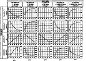
Fig. 1 is the workflow diagram of fractionator;

Fig. 2 is for doing the simulation of fractionator model according to valve position;

Fig. 3 is the diagram result of fractionator factory test;

Fig. 4 is the simulation of fractionator together with the PID controller; And

Fig. 5 is the icon result of the original and recovery value of fractionator.

[figure number explanation]

5 feedbacks are for rate of discharge

6 stoves

7 fractionators

8 PI controllers

9 PI controllers

10 the 3rd PI controllers

11 analyzers

Embodiment

Method of the present invention is the dynamic value that applies to remove from the MPC controller PID controller together with Model Predictive Control.

One MPC processing procedure model belongs to one group of linear equation, so as long as about being present in independence and depending between the variable, any independent variable Ying Keyu depends on the variable exchange on the mathematics.

The combination of accepting conversion be the PID controller settlement (independently) and together with the valve position (depending on) of PID controller.

MPC controller is often based on the linear model of process system.Though invention described herein can be applicable to many-side, the example will be taken from chemical industry and oil refining processing procedure.

The variable that two kinds of forms are all arranged in any system; Be independent variable and depend on variable.Independent variable is the input of system.Independent variable is divided into through control and interference (feedforward) variable.Variable through control is can be by the variable of operator's change, for example valve position or PID controller installation position.Disturbance variable is those independent variables, is powerful in system, but can not be changed by the operator.Variable is for example presented for composition, and feedback is for temperature, and environment temperature etc. is the example of disturbance variable.

Depend on the output that variable is a system.Depend on the influence that variable is changed by independent variable.The operator can not directly change them.Depend on variate-value and controlled, but just passable during the correct change control variable value of mat.Moreover when disturbing invasive system, control variable must correctly be adjusted to resist and disturb.

Use linear model to describe plural number and multiple Variable Control by matrix mathematics.The formula that some MPC models commonly used are arranged now.Wherein a kind of control model commonly used is a step order reaction model:

δ O ₁＝A _1，1Δ I ₁+…+A _1，jΔ I _j+…+A _1，nindΔ I _nind

???????????????????

δ O _i＝A _i，1Δ I ₁+…+A _i,jΔ I _j+…+A _i，nindΔ I _nind

???????????????????

δ O _ndep＝A _ndep，1Δ I ₁+…+A _ndep?jΔ I _j+…+A _ndep，nindΔ I _nind

Formula 1: step order reaction dynamic matrix, square matrix format

Wherein

$\mathrm{\δ}{\stackrel{\‾}{O}}_i=\left[\begin{array}{c}{O}_{i,1}-O_{i,0}\\ O_{i,2}-O_{i,0}\\ O_{i,3}-O_{i,0}\\ \·\\ \·\\ \·\\ O_{i,\mathrm{ncoef}}-O_{i,0}\end{array}\right].$ Depend on the accumulated change of variable the i time in the day part

$\mathrm{\Δ}{\stackrel{\‾}{I}}_j=\left[\begin{array}{c}\mathrm{\Δ}{I}_{j,1}\\ \mathrm{\Δ}{I}_{j,2}\\ \mathrm{\Δ}{I}_{j,3}\\ \·\\ \·\\ \·\\ \mathrm{\Δ}{I}_{j,\mathrm{ncoef}}\end{array}\right],$ The step level of the J time independent variable changes in the day part, and

Dynamic matrix

Equational another form of this step order reaction is finite impulse reaction (FIR) form.As following narration, it can be derived by step order reaction form.

Breathe out by definition again:

b _i，j，k＝a _i，j，k?????????????????for?k＝1，

b _i，j，k＝a _i，j，k-a _{i，j，(k-1)}????for?k:2→ncoef

And

ΔO _i，k＝O _i，k-O _i，(k-1)???????????for?k:1→ncoef

We take off system of equations on the differentiable,

Δ O ₁＝B _1，1Δ I ₁…+B _1，jΔ I _j…+B _1，nindΔ I _nind

???????????????????????????

Δ O _i＝B _i，1Δ I ₁…+B _i，jΔ I _j…+B _i，nindΔ I _nind

???????????????????????????

Δ O _ndep?B _ndep，1Δ I ₁…+B _ndepjΔ I _j…+B _ndep，nindΔ I _nind

Formula 2: finite impulse reaction equation one square matrix format

Wherein

$\mathrm{\Δ}{\stackrel{\‾}{O}}_i=\left[\begin{array}{c}{O}_{i,1}-O_{i,0}\\ O_{i,2}-O_{i,1}\\ O_{i,3}-O_{i,2}\\ \·\\ \·\\ \·\\ O_{i,\mathrm{ncoef}}-O_{i,(\mathrm{ncofe}-1)}\end{array}\right],$ Cross over the variation that the J time of day part depended in the variable

$\mathrm{\Δ}{\stackrel{\‾}{I}}_j=\left[\begin{array}{c}\mathrm{\Δ}{I}_{j,1}\\ \mathrm{\Δ}{I}_{j,2}\\ \mathrm{\Δ}{I}_{j,3}\\ \·\\ \·\\ \·\\ \mathrm{\Δ}{I}_{j,\mathrm{ncoef}}\end{array}\right]$ As above-mentioned situation, and

The model matrix of coefficient of impact

These equations have 5 forms, have only listed the first two here.Because these forms are equal on mathematics, and all forms all can be used for identification prediction and control, they have very different character.

δ O=A Δ I-is most commonly used to control and calculates.

Δ O=B Δ I-is used for the identification of steady state (SS) variable.

Δ Δ O=B Δ Δ I-the be used for identification of oblique line rising variable.

δ O=B δ I-is of little use, and is old-fashioned IDCOM control formula.

Δ O=A Δ Δ I-is of little use.

C.R.Cutler and C.R.Johnston have discussed the character of these matrix formats in paper " analysis of dynamic matrix form ".This paper proposes InstrumentSociety of America ISA85 Advanced in Instrumentation Volume 40.Number 1 in October, 1985.

These linear model The Application of Technology comprise the identification and all in two United States Patent (USP)s 4,349,869 and 4616308 the to some extent descriptions such as control of using and be used for restricted condition of control with model of model.These patent citations in this instructions as a reference.

Derive algorithm of the present invention now to remove the method for PID dynamic value in the explanation slave controller.Begin to derive from the FIR model of formula 2,, suppose the settlement that the J time independent variable is the PID controller now, react for the PID valve that the settlement is changed and depend on variable for the i time in order to derive algorithm.We wish to recombinate model so that make valve become independent variable in the processing procedure model; That is to say that we wish to remove the dynamic value of this PID controller from all affected model reactions.But this mat exchanges and depends on variable for the i time and depend on variable for the J time and finish, as shown below

Wherein Be identity matrix.

Please note that this is that identity matrix multiply by Δ Q ' s to following formula 2.Mat is carried out row and is eliminated calculation,

This can be rewritten as:

$=\left[\begin{array}{c}{\hat{B}}_{\mathrm{1,1}}\\ \·\\ \·\\ \·\\ {\hat{B}}_{(\hat{i}-1),1}\\ {\hat{B}}_{\hat{i},1}\\ {\hat{B}}_{(\hat{i}+1),1}\\ \·\\ \·\\ \·\\ {\hat{B}}_{\mathrm{ndep},1}\end{array}\right]\×\mathrm{\Δ}{\stackrel{\‾}{I}}_1+\…+\left[\begin{array}{c}{\hat{B}}_{1,(\hat{j}-1)}\\ \·\\ \·\\ \·\\ {\hat{B}}_{(\hat{i}-1),(\hat{j}-1)}\\ {\hat{B}}_{\hat{i},(\hat{j}-1)}\\ {\hat{B}}_{(\hat{i}+1),(\hat{j}-1)}\\ \·\\ \·\\ \·\\ {\hat{B}}_{\mathrm{ndep},(\hat{j}-1)}\end{array}\right]\×\mathrm{\Δ}{\stackrel{\‾}{I}}_{(\hat{j}-1)}+\left[\begin{array}{c}0\\ \·\\ \·\\ \·\\ 0\\ -I\\ 0\\ \·\\ \·\\ \·\\ 0\end{array}\right]\×\mathrm{\Δ}{\stackrel{\‾}{I}}_{\hat{j}}+\left[\begin{array}{c}{\hat{B}}_{1,(\hat{j}+1)}\\ \·\\ \·\\ \·\\ {\hat{B}}_{(\hat{i}-1),(\hat{j}+1)}\\ {\hat{B}}_{\hat{j},(\hat{j}+1)}\\ {\hat{B}}_{(\hat{i}+1),(\hat{j}+1)}\\ \·\\ \·\\ \·\\ {\hat{B}}_{\mathrm{ndep},(\hat{j}+1)}\end{array}\right]\×\mathrm{\Δ}{\stackrel{\‾}{I}}_{(\hat{j}+1)}\…+\left[\begin{array}{c}{\hat{B}}_{1,\mathrm{nind}}\\ \·\\ \·\\ \·\\ {\hat{B}}_{(\hat{i}-1),\mathrm{nind}}\\ {\hat{B}}_{\hat{i},\mathrm{nind}}\\ {\hat{B}}_{(\hat{i}+1),\mathrm{nind}}\\ \·\\ \·\\ \·\\ {\hat{B}}_{\mathrm{ndep},\mathrm{nind}}\end{array}\right]\×\mathrm{\Δ}{\stackrel{\‾}{I}}_{\mathrm{nind}}$

$=\left[\begin{array}{c}I\\ \·\\ \·\\ \·\\ 0\\ 0\\ 0\\ \·\\ \·\\ \·\\ 0\end{array}\right]\×\mathrm{\Δ}{\stackrel{\‾}{O}}_1+\…+\left[\begin{array}{c}0\\ \·\\ \·\\ \·\\ I\\ 0\\ 0\\ \·\\ \·\\ \·\\ 0\end{array}\right]\×\mathrm{\Δ}{\stackrel{\‾}{O}}_{(\hat{i}-1)}+\left[\begin{array}{c}-{\hat{B}}_{1,\hat{j}}\\ \·\\ \·\\ \·\\ -{\hat{B}}_{(\hat{i}-1),\hat{j}}\\ -{\hat{B}}_{\hat{i},\hat{j}}\\ {\widehat{-B}}_{(\hat{i}+1),\hat{j}}\\ \·\\ \·\\ \·\\ -{\hat{B}}_{\mathrm{ndep},\hat{j}}\end{array}\right]\×\mathrm{\Δ}{\stackrel{\‾}{O}}_{\hat{i}}+\left[\begin{array}{c}0\\ \·\\ \·\\ \·\\ 0\\ 0\\ I\\ \·\\ \·\\ \·\\ 0\end{array}\right]\×\mathrm{\Δ}{\stackrel{\‾}{O}}_{(\hat{i}+1)}+\…+\left[\begin{array}{c}0\\ \·\\ \·\\ \·\\ 0\\ 0\\ 0\\ \·\\ \·\\ \·\\ I\end{array}\right]\×\mathrm{\Δ}{\stackrel{\‾}{O}}_{\mathrm{ndep}}$

Maybe can be rearranged to

$\left[\begin{array}{c}{\hat{B}}_{\mathrm{1,1}}\\ \·\\ \·\\ \·\\ {\hat{B}}_{(\hat{i}-1),1}\\ {\hat{B}}_{\hat{i},1}\\ {\hat{B}}_{(\hat{i}+1),1}\\ \·\\ \·\\ \·\\ {\hat{B}}_{\mathrm{ndep},1}\end{array}\right]$ ${\stackrel{\‾}{I}}_1$ $\left[\begin{array}{c}{\hat{B}}_{1,(\hat{j}-1)}\\ \·\\ \·\\ \·\\ {\hat{B}}_{(\hat{i}-1),(\hat{j}-1)}\\ {\hat{B}}_{\hat{i},(\hat{j}-1)}\\ {\hat{B}}_{(\hat{i}+1),(\hat{j}-1)}\\ \·\\ \·\\ \·\\ {\hat{B}}_{\mathrm{ndep},(\hat{j}-1)}\end{array}\right]$ ${\stackrel{\‾}{I}}_{(\hat{j}-1)}$ $+\left[\begin{array}{c}{\hat{B}}_{1,(\hat{j}+1)}\\ \·\\ \·\\ \·\\ {\hat{B}}_{(\hat{i}-1),\hat{j}}\\ {\hat{B}}_{\hat{i},\hat{j}}\\ {\hat{B}}_{(\hat{i}+1),\hat{j}}\\ \·\\ \·\\ \·\\ {\hat{B}}_{\mathrm{ndep},\hat{j}}\end{array}\right]\×\mathrm{\Δ}{\stackrel{\‾}{O}}_{\hat{i}}+\left[\begin{array}{c}{\hat{B}}_{1,(\hat{j}+1)}\\ \·\\ \·\\ \·\\ {\hat{B}}_{(\hat{i}-1),(\hat{j}+1)}\\ {\hat{B}}_{\hat{i},(\hat{j}+1)}\\ {\hat{B}}_{(\hat{i}+1),(\hat{j}+1)}\\ \·\\ \·\\ \·\\ {\hat{B}}_{\mathrm{ndep},(\hat{j}+1)}\end{array}\right]\×\mathrm{\Δ}{\stackrel{\‾}{I}}_{(\hat{j}+1)}\…+\left[\begin{array}{c}{\hat{B}}_{1,\mathrm{nind}}\\ \·\\ \·\\ \·\\ {\hat{B}}_{(\hat{i}-1),\mathrm{nind}}\\ {\hat{B}}_{\hat{i},\mathrm{nind}}\\ {\hat{B}}_{(\hat{i}+1),\mathrm{nind}}\\ \·\\ \·\\ \·\\ {\hat{B}}_{\mathrm{ndep},\mathrm{nind}}\end{array}\right]\×\mathrm{\Δ}{\stackrel{\‾}{I}}_{\mathrm{nind}}$

$=\left[\begin{array}{c}I\\ \·\\ \·\\ \·\\ 0\\ 0\\ 0\\ \·\\ \·\\ \·\\ 0\end{array}\right]\×\mathrm{\Δ}{\stackrel{\‾}{O}}_1+\…+\left[\begin{array}{c}0\\ \·\\ \·\\ \·\\ I\\ 0\\ 0\\ \·\\ \·\\ \·\\ 0\end{array}\right]\×\mathrm{\Δ}{\stackrel{\‾}{O}}_{(\hat{i}-1)}+\left[\begin{array}{c}0\\ \·\\ \·\\ \·\\ 0\\ I\\ 0\\ \·\\ \·\\ \·\\ 0\end{array}\right.\×\mathrm{\Δ}{\stackrel{\‾}{I}}_{\hat{j}}+\left[\begin{array}{c}0\\ \·\\ \·\\ \·\\ 0\\ 0\\ I\\ \·\\ \·\\ \·\\ 0\end{array}\right]\×\mathrm{\Δ}{\stackrel{\‾}{O}}_{(\hat{i}+1)}+\…+\left[\begin{array}{c}0\\ \·\\ \·\\ \·\\ 0\\ 0\\ 0\\ \·\\ \·\\ \·\\ I\end{array}\right]\×{\mathrm{\Δ}\stackrel{\‾}{O}}_{\mathrm{ndep}}$

Or organize separately the matrix equation formula synthetic:

Please note Δ O _iWith Δ I _jExchanged, therefore now valve position become one independently variable PID settlement then become and depend on variable.This has only illustrated and has removed the PID dynamic value from a PID controller, but obviously is general multiple independence/depend on variable can be joined the dynamic value that exchange removes multiple controller by this in calculation.

Utilize now numeral illustrate an example how on earth adopting said method remove dynamic value in the special PID controller in model predictive controller.

Suppose-FIR has 2 independent variables, and 2 is attached variable and 4 model coefficients, and second settlement that independent variable is the PID controller, and second is depended on the valve position that variable is the PID controller.Our intended for reconstitution model and its PID valve position is changed to independent variable rather than PID settlement.This need remove according to above-mentioned algorithm the dynamic value of PID controller from all system responses.This example is equally to equation Δ O=B Δ I _i, δ O=B δ I, and Δ Δ O=B Δ Δ I form is effective.

Depend on weary-1

Independent weary-1Independent weary-2

b _1，1，1＝1.5????b _1，2，1＝0.5

b _1，1，2＝0.6????b _1，2，2＝0.4

b _1，1，3＝0.2????b _1，2，3＝0.2

b _1，1，4＝0.1????b _1，2，4＝0.1

Be attached weary-2

Independent weary-1Independent weary-2

b _2，1，1＝-0.3????????????b _2，2，1＝0.75

b _2，1，2＝-0.4????????????b _2，2，2＝0.25

b _2，1，3＝-0.1????????????b _2，2，3＝0.15

b _2，1，4＝-0.05???????????b _2，2，4＝0.05

This problem goes out at following column matrix middle finger.

Point out the pivot key element

??1.5??????0????????0??????0 ??0.6??????1.5??????0??????0 ??0.2??????0.6??????1.5????0 ??0.1??????0.2??????0.6????1.5	?0.5???0??????0??????0 ?0.4???0.5????0??????0 ?0.2???0.4????0.5????0 ?0.1???0.2????0.4????0.5	??1???0???0??0 ??0???1???0??0 ??0???0???1??0 ??0???0???0??1	????0???0??0????0 ????0???0??0????0 ????0???0??0????0 ????0???0??0????0
				??-0.3?????0????????0??????0 ??-0.4?????-0.3?????0??????0 ??-0.1?????-0.4?????-0.3???0 ??-0.05????-0.1?????-0.4???-0.3	?0.75??0??????0??????0 ?0.25??0.75???0??????0 ?0.15??0.25???0.75???0 ?0.05??0.15???0.25???0.75	??0???0???0??0 ??0???0???0??0 ??0???0???0??0 ??0???0???0??0	????1???0??0????0 ????0???1??0????0 ????0???0??1????0 ????0???0??0????1

Formula 5 multiply by (1/0.75)

????1.5????0??????0??????0 ????0.6????1.5????0??????0 ????0.2????0.6????1.5????0 ????0.1????0.2????0.6????1.5	??0.5???0??????0??????0 ??0.4???0.5????0??????0 ??0.2???0.4????0.5????0 ??0.1???0.2????0.4????0.5	??1???0???0???0 ??0???1???0???0 ??0???0???1???0 ??0???0???0???1	0??????0??0??0 0??????0??0??0 0??????0??0??0 0??????0??0??0
				????0.4????0??????0??????0 ????-0.4???-0.3???0??????0 ????-0.1???-0.4???-0.3???0 ????-0.05??-0.1???-0.4???-0.3	??-1????0??????0??????0 ??0.25??0.75???0??????0 ??0.15??0.25???0.75???0 ??0.05??0.15???0.25???0.75	??0???0???0???0 ??0???0???0???0 ??0???0???0???0 ??0???0???0???0	-1.333?0??0??0 0??????1??0??0 0??????0??1??0 0??????0??0??1

Formula 5 multiply by 0.5, adds in formula 1 and replacement formula 1

Formula 5 multiply by 0.4, adds in formula 2 and replacement formula 2

Formula 5 multiply by 0.2, adds in formula 3 and replacement formula 3

Formula 5 multiply by 0.1, adds in formula 4 and replacement formula 4

Formula 5 multiply by 0.25, adds in formula 6 and replacement formula 6

Formula 5 multiply by 0.15, adds in formula 7 and replacement formula 7

Formula 5 multiply by 0.05, adds in formula 8 and replacement formula 8

????1.7????0??????0??????0 ????0.76???1.5????0??????0 ????0.28???0.6????1.5????0 ????0.14???0.2????0.6????1.5	???0?????0??????0??????0 ???0????0.5?????0??????0 ???0????0.4?????0.5????0 ???0????0.2?????0.4????0.5	????1????0????0????0 ????0????1????0????0 ????0????0????1????0 ????0????0????0????1	????-0.667??0????0????0 ????-0.533??0????0????0 ????-0.267??0????0????0 ????-0.133??0????0????0
				????0.4????0??????0??????0 ????-0.3???-0.3???0??????0 ????-0.04??-0.4???-0.3???0 ????-0.03??-0.1???-0.4???-0.3	???-1???0???????0??????0 ???0????0.75????0??????0 ???0????0.25????0.75???0 ???0????0.15????0.25???0.75	????0????0????0????0 ????0????0????0????0 ????0????0????0????0 ????0????0????0????0	????-1.333??0????0????0 ????-0.333??1????0????0 ????-0.2????0????1????0 ????-0.067??0????0????1

Formula 6 multiply by (1/0.75)

??1.7?????0??????0???????0 ??0.76????1.5????0???????0 ??0.28????0.6????1.5?????0 ??0.14????0.2????0.6?????1.5	????0????0??????0???????0 ????0????0.5????0???????0 ????0????0.4????0.5?????0 ????0????0.2????0.4?????0.5	????1????0????0????0 ????0????1????0????0 ????0????0????1????0 ????0????0????0????1	??-0.667????0??????0???0 ??-0.533????0??????0???0 ??-0.267????0??????0???0 ??-0.133????0??????0???0
				??0.4?????0??????0???????0 ??0.4?????0.4????0???????0 ??-0.04???-0.4???-0.3????0 ??-0.03???-0.1???-0.4????-0.3	????-1???0??????0???????0 ????0????-1?????0???????0 ????0????0.25???0.75????0 ????0????0.15???0.25????0.75	????0????0????0????0 ????0????0????0????0 ????0????0????0????0 ????0????0????0????0	???-1.333???0??????0???0 ???0.444????-1.333?0???0 ???-0.2?????0??????1???0 ???-0.067???0??????0???1

Formula 5 multiply by 0.5, adds in formula 2 and replacement formula 2

Formula 5 multiply by 0.4, adds in formula 3 and replacement formula 3

Formula 5 multiply by 0.2, adds in formula 4 and replacement formula 4

Formula 5 multiply by 0.25, adds in formula 7 and replacement formula 7

Formula 5 multiply by 0.15, adds in formula 8 and replacement formula 8

??1.7???0??????0??????0 ??0.96??1.7????0??????0 ??0.44??0.76???1.5????0 ??0.22??0.28???0.6????1.5	??0????0????0???????0 ??0????0????0???????0 ??0????0????0.5?????0 ??0????0????0.4?????0.5	????1????0????0????0 ????0????1????0????0 ????0????0????1????0 ????0????0????0????1	??-0.667??0???????0??0 ??-0.311??-0.667??0??0 ??-0.089??-0.533??0??0 ??-0.044??-0.267??0??0
				??0.4???0??????0??????0 ??0.4???0.4????0??????0 ??0.06??-0.3???-0.3???0 ??0.03??-0.04??-0.4???-0.3	??-1???0????0???????0 ??0????-1???0???????0 ??0????0????0.75????0 ??0????0????0.25????0.75	????0????0????0????0 ????0????0????0????0 ????0????0????0????0 ????0????0????0????0	??-1.333??0???????0??0 ??0.444???-1.333??0??0 ??-0.089??-0.333??1??0 ??0???????-0.2????0??1

Formula 7 multiply by (1/0.75)

????1.7????0????0????0

?0????0????0????0

?1????0????0????0

-0.667????0????0????0

??0.96???1.7????0??????0 ??0.44???0.76???1.5????0 ??0.22???0.28???0.6????1.5	??0????0????0?????0 ??0????0????0.5???0 ??0????0????0.4???0.5	????0????1????0????0 ????0????0????1????0 ????0????0????0????1	-0.311??-0.667????0???????0 -0.089??-0.533????0???????0 -0.044??-0.267????0???????0
				??0.4????0??????0??????0 ??0.4????0.4????0??????0 ??-0.08??0.4????0.4????0 ??0.03???-0.04??-0.4???-0.3	??-1???0????0?????0 ??0????-1???0?????0 ??0????0????-1????0 ??0????0????0.25??0.75	????0????0????0????0 ????0????0????0????0 ????0????0????0????0 ????0????0????0????0	-1.333??0?????????0???????0 0.444???-1.333????0???????0 0.119???0.4444????-1.333??0 0???????-0.2??????0???????1

Formula 5 multiply by 0.5, adds in formula 3 and replacement formula 3

Formula 5 multiply by 0.4, adds in formula 4 and replacement formula 4

Formula 5 multiply by 0.25, adds in formula 8 and replacement formula 8

??1.7????0??????0??????0 ??0.96???1.7????0??????0 ??0.4????0.96???1.7????0 ??0.188??0.44???0.76???1.5	????0????0????0????0 ????0????0????0????0 ????0????0????0????0 ????0????0????0????0.5	????1????0????0????0 ????0????1????0????0 ????0????0????1????0 ????0????0????0????1	-0.667??0???????0?????????0 -0.311??-0.667??0?????????0 -0.030??-0.311??-0.667????0 0.003???-0.089??-0.533????0
				??0.4????0??????0??????0 ??0.4????0.4????0??????0 ??-0.08??0.4????0.4????0 ??0.01???0.06???-0.3???-0.3	????-1???0????0????0 ????0????-1???0????0 ????0????0????-1???0 ????0????0????0????0.75	????0????0????0????0 ????0????0????0????0 ????0????0????0????0 ????0????0????0????0	-1.333??0???????0?????????0 0.444???-1.333??0?????????0 0.119???0.444???-1.333????0 0.030???-0.089??-0.333????1

Formula 8 multiply by (1/0.75)

??1.7?????0??????0??????0 ??0.96????1.7????0??????0 ??0.4?????0.96???1.7????0 ??0.188???0.44???0.76???1.5	??0????0????0????0 ??0????0????0????0 ??0????0????0????0 ??0????0????0????0.5	??1????0????0????0 ??0????1????0????0 ??0????0????1????0 ??0????0????0????1	??-0.667??0????????0?????????0 ??-0.311??-0.667???0?????????0 ??-0.030??-0.311???-0.667????0 ??0.003???-0.089???-0.533????0
				??0.4?????0??????0??????0 ??0.4?????0.4????0??????0 ??-0.08???0.4????0.4????0 ??-0.013??-0.08??0.4????0.4	??-1???0????0????0 ??0????-1???0????0 ??0????0????-1???0 ??0????0????0????-1	??0????0????0????0 ??0????0????0????0 ??0????0????0????0 ??0????0????0????0	??-1.333??0????????0?????????0 ??0.444???-1.333???0?????????0 ??0.119???0.444????-1.333????0 ??-0.040??0.119????0.444?????-1.333

Formula 5 multiply by 0.5, adds in formula 4 and replacement formula 4

1.7??????0??????0?????0 0.96?????1.7????0?????0 0.4??????0.96???1.7???0 0.181????0.4????0.96??1.7	????0????0????0????0 ????0????0????0????0 ????0????0????0????0 ????0????0????0????0	????1????0????0????0 ????0????1????0????0 ????0????0????1????0 ????0????0????0????1	????-0.667??0?????????0????????0 ????-0.311??-0.667????0????????0 ????-0.030??-0.311????-0.667???0 ????-0.017??-0.030????-0.311???-0.667
				0.4??????0??????0?????0 0.4??????0.4????0?????0 -0.08????0.4????0.4???0 -0.01 3????????-0.08??0.4???0.4	????-1???0????0????0 ????0????-1???0????0 ????0????0????-1???0 ????0????0????0???-1	????0????0????0????0 ????0????0????0????0 ????0????0????0????0 ????0????0????0????0	????-1.333??0?????????0????????0 ????0.444???-1.333????0????????0 ????0.119???0.444?????-1.333???0 ????-0.040??0.119?????0.444????-1.333

Rearrange equation

????1.7????0????0????0

?0.667????0????0????0

??1????0????0????0

?0????0????0????0

??0.96????1.7???0????0 ??0.4?????0.96??1.7??0 ??0.181???0.4???0.96?1.7	0.311???0.667????0???????0 0.030???0.311????0.667???0 0.017???0.030????0.311???0.667	????0????1????0????0 ????0????0????1????0 ????0????0????0????1	????0????0????0????0 ????0????0????0????0 ????0????0????0????0
				??0.4?????0?????0????0 ??0.4?????0.4???0????0 ??-0.08???0.4???0.4??0	1.333???0????????0???????0 -0.444??1.333????0???????0 -0.119??-0.444??1.333????0	????0????0????0????0 ????0????0????0????0 ????0????0????0????0	????1????0????0????0 ????0????1????0????0 ????0????0????1????0

The new model coefficient that PID removes after the dynamic value is as follows:

Be attached weary-1

Independent weary-1 Independent weary-2

 _1，1，1＝1.7????????????? _1，2，1＝0.667

 _1，1，2＝0.96???????????? _1，2，2＝0.311

 _1，1，3＝0.4????????????? _1，2，3＝0.030

 _1，1，4＝0.181??????????? _1，2，4＝0.017

Depend on weary-2

Independent weary-1 Independent weary-2

 _2，1，1＝0.4?????????????? _2，2，1＝1.333

 _2，1，2＝0.4?????????????? _2，2，2＝-0.444

 _2，1，3＝-0.08???????????? _2，2，3＝-0.119

 _2，1，4＝-0.0133?????????? _2，2，4＝0.040

Please note that all coefficient values have all become, this new controller has had the dynamic value after second independent variable (PID settlement) removes now.This controller can be used to now control processing procedure and the exploitation of this controller be used as off-line with and must on processing procedure, not carry out another time-consuming and expensive identification test.

[remove the algorithm of PID dynamic value, open loop step order reaction form]

Derive with example in, we discussed from one based on impact or the equation form of derivative FIR model remove the algorithm of PID dynamic value.Same algorithm can be model δ O=A Δ I and goes on foot the derivation of a level coefficient form, and just individual now independent, 2 examples that depend on variable are done explanation.For the purpose of this example, we suppose that second independently should exchange with second value of depending on.Problem can be listed as follows by matrix format:

$\left[\begin{array}{cc}{A}_{\mathrm{1,1}}& {\mathrm{<figure-callout\; id="1"\; label="A"\; filenames="A0380348200421.png,A0380348200451.png"\; state="\{\{state\}\}">A</figure-callout>}}_{\mathrm{1,2}}\\ {\mathrm{<figure-callout\; id="2"\; label="A"\; filenames="A0380348200451.png"\; state="\{\{state\}\}">A</figure-callout>}}_{\mathrm{2,1}}& {\mathrm{<figure-callout\; id="2"\; label="A"\; filenames="A0380348200451.png"\; state="\{\{state\}\}">\; <figure-callout\; id="2"\; label="A"\; filenames="A0380348200451.png"\; state="\{\{state\}\}">A</figure-callout>\; </figure-callout>}}_{\mathrm{2,2}}\end{array}\right]\&times;\left[\begin{array}{c}\mathrm{\&Delta;}{\stackrel{\&OverBar;}{I}}_1\\ \mathrm{\&Delta;}{\stackrel{\&OverBar;}{I}}_2\end{array}\right]=\left[\begin{array}{c}I0\\ 0I\end{array}\right]\&times;\left[\begin{array}{c}\mathrm{\&delta;}{\stackrel{\&OverBar;}{O}}_1\\ \mathrm{\&delta;}{\stackrel{\&OverBar;}{O}}_2\end{array}\right]$

Finish and eliminate operation (pivotal method),

$\left[\begin{array}{cc}{\hat{A}}_{\mathrm{1,1}}& 0\\ {\hat{B}}_{\mathrm{2,1}}& -I\end{array}\right]\&times;\left[\begin{array}{c}\mathrm{\&Delta;}{\stackrel{\&OverBar;}{I}}_1\\ \mathrm{\&Delta;}{\stackrel{\&OverBar;}{I}}_2\end{array}\right]=\left[\begin{array}{c}I-{\hat{B}}_{\mathrm{1,2}}\\ 0-{\hat{C}}_{\mathrm{2,2}}\end{array}\right]\&times;\left[\begin{array}{c}\mathrm{\&delta;}{\stackrel{\&OverBar;}{O}}_1\\ \mathrm{\&delta;}{\stackrel{\&OverBar;}{O}}_2\end{array}\right]$

Rearrange:

$\left[\begin{array}{cc}{\hat{A}}_{\mathrm{1,1}}& {\hat{B}}_{\mathrm{1,2}}\\ {\hat{B}}_{\mathrm{2,1}}& {\hat{C}}_{\mathrm{2,2}}\end{array}\right]\&times;\left[\begin{array}{c}\mathrm{\&Delta;}{\stackrel{\&OverBar;}{I}}_1\\ \mathrm{\&delta;}{\stackrel{\&OverBar;}{O}}_2\end{array}\right]=\left[\begin{array}{c}I0\\ 0I\end{array}\right]\&times;\left[\begin{array}{c}\mathrm{\&delta;}{\stackrel{\&OverBar;}{O}}_1\\ \mathrm{\&Delta;}{\stackrel{\&OverBar;}{I}}_2\end{array}\right]$

Can write:

${\hat{A}}_{\mathrm{1,1}}\mathrm{\&Delta;}{\stackrel{\&OverBar;}{I}}_1+{\hat{B}}_{\mathrm{1,2}}\mathrm{\&delta;}{\stackrel{\&OverBar;}{O}}_2=\mathrm{\&delta;}{\stackrel{\&OverBar;}{O}}_1$

${\hat{B}}_{\mathrm{2,1}}\mathrm{\&Delta;}{\stackrel{\&OverBar;}{I}}_1+{\hat{C}}_{\mathrm{2,2}}\mathrm{\&delta;}{\stackrel{\&OverBar;}{O}}_2=\mathrm{\&Delta;}{\stackrel{\&OverBar;}{I}}_2$

Please remember that coefficient of impact is defined as:

b _i，j，k＝a _i，j，k????????????????????????????for?k＝1

b _i，j，k＝a _i，j，k-a _{i，j，(k-1)}＝Δa _i，j，k???for?k:2→ncoef

In like manner, defining the second different coefficients now is:

c _i，j，k＝b _i，j，k????????????????????????????for?k＝1

c _i，j，k＝b _i，j，k-b _{i，j，(k-1)}＝Δb _i，j，k???for?k:2→ncoef

Note

$b_{i,j,m}=\underset{m=1}{\overset{l}{\mathrm{\&Sigma;}}}\left(c_{i,j,l}\right)$

$a_{i,j,k}=\underset{l=1}{\overset{k}{\mathrm{\&Sigma;}}}\left(b_{i,j,l}\right)=\underset{l}{\overset{k}{\mathrm{\&Sigma;}}}\left(\underset{m=1}{\overset{l}{\mathrm{\&Sigma;}}}\left(c_{i,j,m}\right)\right)$

Please note that present matrix becomes step order reaction coefficient (A), coefficient of impact (B), and the mixing of the different coefficients of secondary (C) is closed.Because new independent variable belongs to " accumulation " form rather than " difference quotient " form, and the new variable that depends on belongs to " difference quotient " form but not " accumulation " form.Become a step level form and use and recover a step level coefficient in order to change this system of equations, just need carry out following two steps:

Step 1: change new independent variable by " accumulation " to " difference quotient " form, δ O ₂ Δ O ₂

Step 2: change and new depend on variable by " difference quotient " to " accumulation " form, Δ I ₂ δ I ₂

Step 1: change new independent variable by " accumulation " to " difference quotient ".

This step need only rearrange every in the equation, note that δ O ₂In this matrix, come across two sections:

Because

b _{I, j, k}=a _{I, j, k}K=1 Time

b _{I, j, k}=a _{I, j, k}-a _{I, j, (k-1)}=Δ a _{I, j, k}K:2 → ncoef Time

And

c _{I, j, k}=b _{I, j, k}K=1 Time

c _{I, j, k}=b _{I, jk}-b _{I, j, (k-1)}=Δ b _{I, j, k}K:2 → ncoef Time

We can be write as following formula:

$=\left[\begin{array}{c}{\hat{a}}_{\mathrm{1,2,1}}(O_{\mathrm{2,1}}-O_{\mathrm{2,0}})\\ {\hat{a}}_{\mathrm{1,2,2}}{O}_{\mathrm{2,1}}-{\hat{a}}_{\mathrm{1,2,2}}{O}_{\mathrm{2,0}}-{\hat{a}}_{\mathrm{1,2,1}}{O}_{\mathrm{2,1}}+{\hat{a}}_{\mathrm{1,2,1}}{O}_{\mathrm{2,0}}+{\hat{a}}_{\mathrm{1,2,1}}{O}_{\mathrm{2,2}}-{\hat{a}}_{\mathrm{1,2,1}}{O}_{\mathrm{2,0}}\\ {\hat{a}}_{\mathrm{1,2,3}}{O}_{\mathrm{2,1}}-{\hat{a}}_{\mathrm{1,2,3}}{O}_{\mathrm{2,0}}-{\hat{a}}_{\mathrm{1,2,2}}{O}_{2,1}+{\hat{a}}_{\mathrm{1,2,2}}{O}_{2,0}+{\hat{a}}_{\mathrm{1,2,2}}{O}_{2,2}-{\hat{a}}_{\mathrm{1,2,2}}{O}_{2,0}-{\hat{a}}_{\mathrm{1,2,2}}{O}_{\mathrm{2,2}}+{\hat{a}}_{\mathrm{1,2,1}}{O}_{\mathrm{2,0}}+{\hat{a}}_{\mathrm{1,2},1}{O}_{\mathrm{2,3}}-{\hat{a}}_{\mathrm{1,2,1}}{O}_{\mathrm{2,0}}\\ \&CenterDot;\\ \&CenterDot;\\ \&CenterDot;\\ {\hat{b}}_{\mathrm{2,2,1}}(O_{\mathrm{2,1}}-O_{\mathrm{2,0}})\\ {\hat{b}}_{\mathrm{2,2,2}}{O}_{\mathrm{2,1}}-{\hat{b}}_{\mathrm{2,2,2}}{O}_{\mathrm{2,0}}-{\hat{b}}_{\mathrm{2,2,1}}{O}_{\mathrm{2,1}}+{\hat{b}}_{\mathrm{2,2,1}}{O}_{\mathrm{2,0}}+{\hat{b}}_{\mathrm{2,2,1}}{O}_{\mathrm{2,2}}-{\hat{b}}_{\mathrm{2,2,1}}{O}_{\mathrm{2,0}}\\ {\hat{b}}_{\mathrm{2,2,3}}{O}_{\mathrm{2,1}}-{\hat{b}}_{\mathrm{2,2,3}}{O}_{\mathrm{2,0}}-{\hat{b}}_{\mathrm{2,2,2}}{O}_{\mathrm{2,1}}+{\hat{b}}_{\mathrm{2,2,2}}{O}_{2,0}+{\hat{b}}_{\mathrm{2,2,2}}{O}_{\mathrm{2,2}}-{\hat{b}}_{\mathrm{2,2,2}}{O}_{\mathrm{2,0}}-{\hat{b}}_{\mathrm{2,2,1}}{O}_{\mathrm{2,2}}+{\hat{b}}_{\mathrm{2,2,1}}{O}_{\mathrm{2,0}}\\ \&CenterDot;\\ \&CenterDot;\\ \&CenterDot;\end{array}\right]$

$=\left[\begin{array}{c}{\hat{a}}_{\mathrm{1,2,1}}(O_{\mathrm{2,1}}-O_{\mathrm{2,0}})\\ {\hat{a}}_{\mathrm{1,2,2}}(O_{\mathrm{2,1}}-O_{\mathrm{2,0}})+{\hat{a}}_{\mathrm{1,2,1}}(O_{\mathrm{2,2}}-O_{\mathrm{2,1}}+O_{\mathrm{2,0}}-O_{\mathrm{2,0}})\\ {\hat{a}}_{\mathrm{1,2,3}}(O_{\mathrm{2,1}}-O_{\mathrm{2,0}})+{\hat{a}}_{\mathrm{1,2,2}}(O_{\mathrm{2,2}}-O_{\mathrm{2,1}}+O_{\mathrm{2,0}}-O_{\mathrm{2,0}})+{\hat{a}}_{\mathrm{1,2,1}}(O_{\mathrm{2,3}}-O_{\mathrm{2,2}}+O_{\mathrm{2,0}}-O_{\mathrm{2,0}})\\ \&CenterDot;\\ \&CenterDot;\\ \&CenterDot;\\ {\hat{b}}_{\mathrm{2,2,1}}(O_{\mathrm{2,1}}-O_{\mathrm{2,0}})\\ {\hat{b}}_{\mathrm{2,2,2}}(O_{\mathrm{2,1}}-O_{\mathrm{2,0}})+{\hat{b}}_{\mathrm{2,2,1}}(O_{\mathrm{2,2}}-O_{\mathrm{2,1}}+O_{\mathrm{2,0}}-O_{\mathrm{2,0}})\\ {\hat{b}}_{\mathrm{2,2,3}}(O_{\mathrm{2,1}}-O_{\mathrm{2,0}})+{\hat{b}}_{\mathrm{2,2,2}}(O_{\mathrm{2,2}}-O_{\mathrm{2,1}}+O_{\mathrm{2,0}}-O_{\mathrm{2,0}})+{\hat{b}}_{\mathrm{2,2,1}}(O_{\mathrm{2,3}}-O_{\mathrm{2,2}}+O_{\mathrm{2,0}}-O_{\mathrm{2,0}})\\ \&CenterDot;\\ \&CenterDot;\\ \&CenterDot;\end{array}\right]$

Because $\left[\begin{array}{cc}{\hat{B}}_{\mathrm{1,2}}& \mathrm{\&delta;}{\stackrel{\&OverBar;}{O}}_2\\ {\hat{C}}_{\mathrm{2,2}}& \mathrm{\&delta;}{\stackrel{\&OverBar;}{O}}_2\end{array}\right]=\left[\begin{array}{cc}{\hat{A}}_{\mathrm{1,2}}& \mathrm{\&Delta;}{\stackrel{\&OverBar;}{O}}_2\\ {\hat{B}}_{\mathrm{2,2}}& \mathrm{\&Delta;}{\stackrel{\&OverBar;}{O}}_2\end{array}\right]$ We can rewrite this system of equations:

${\hat{A}}_{\mathrm{1,1}}\mathrm{\&Delta;}{\stackrel{\&OverBar;}{I}}_1+{\hat{A}}_{\mathrm{1,2}}\mathrm{\&Delta;}{\stackrel{\&OverBar;}{O}}_2=\mathrm{\&delta;}{\stackrel{\&OverBar;}{O}}_1$

${\hat{B}}_{\mathrm{2,1}}\mathrm{\&Delta;}{\stackrel{\&OverBar;}{I}}_1+{\hat{B}}_{\mathrm{2,2}}\mathrm{\&Delta;}{\stackrel{\&OverBar;}{O}}_2=\mathrm{\&Delta;}{\stackrel{\&OverBar;}{I}}_2$

So far completing steps 1.

Step 2: conversion is newly depended on variable by " differential " to " accumulation " form

New second depends on the variable equation is write as followsly, need convert these equations to " accumulation " form by " difference quotient ".

 _2，1，1ΔI _1，1???????????????????????????????????????????????????+ _2，2，1ΔO _2，1????????????????????????????????????????????????＝I _2，1-I _2，0＝ΔI _2，1

 _2，1，2ΔI _1，1+ _2，1，1ΔI _1，2??????????????????????????????????+ _2，2，2ΔO _2，1+ _2，2，1ΔO _2，2????????????????????????????????＝I _2，2-I _2，1＝ΔI _2，2

 _2，1，3ΔI _1，1+ _2，1，2ΔI _1，2+ _2，1，1ΔI _1，3?????????????????+ _2，2，3ΔO _2，1+ _2，2，2ΔO _2，2+ _2，2，1ΔO _2，3????????????????＝I _2，3-I _2，2＝ΔI _2，3

 _2，1，4ΔI _1，1+ _2，1，3ΔI _1，2+ _2，1，2ΔI _1，3+ _2，1，1ΔI _1，4+ _2，2，4ΔO _2，1+ _2，2，3ΔO _2，2+ _2，2，2ΔO _2，3+ _2，2，1ΔO _2，4＝I _2，4-I _2，3＝ΔI _2，4

??????????????????????????????????????????????????????????????????????????????????????????????????????????????????????????????

Because according to definition b _{I, j, 1}=a _{I, j, 1}And I _{J, 1}-I _{J, 0}=Δ I _{J, 1}=δ I _{J, 1}Formula 1 becomes

_2，1，1ΔI _1，1+ _2，2，1ΔO _2，1＝δI _2，1

In order to try to achieve second a step level coefficient equation, two coefficient of impact equations at first should be added up:

( _2，1，1+ _2，1，2)ΔI _1，1+ _2，1，1ΔI _1，2+( _2，2，1+ _2，2，2)ΔO _2，1+ _2，2，1ΔO _2，2＝I _2，2-I _2，1+I _2，1-I _2，0＝I _2，2-I _2，0

Or

_2，1，2ΔI _1，1+ _2，1，1ΔI _1，2+ _2，2，2ΔO _2，1+ _2，2，1ΔO _2，2＝δI _2，2

In order to try to achieve second a step level coefficient equation, 3 coefficient of impact equations at first should be added up:

( _2，1，1+ _2，1，2+ _2，1，3)ΔI _1，1+( _2，1，1+ _2，1，2)ΔI _1，2+ _2，1，1ΔI _1，3

+( _2，2，1+ _2，2，2+ _2，2，3)ΔO _2，1+( _2，2，1+ _2，2，2)ΔO _2，2+ _2，2，1ΔO _2，3

＝I _2，3-I _2，2+I _2，2-I _2，1+I _2，1-I _2，0＝I _2，3-I _2，0

Or,

_2，1，3ΔI _1，1+ _2，1，2ΔI _1，2+ _2，1，1ΔI _1，3+ _2，2，3ΔO _2，1+ _2，2，2ΔO _2，2+ _2，2，1ΔO _2，3＝δI _2，3

In order to try to achieve the mat woven of fine bamboo strips four a step level coefficient equation, 4 coefficient of impact equations at first should be added up:

( _2，1，1+ _2，1，2+ _2，1，3+ _2，1，4)ΔI _1，1+( _2，1，1+ _2，1，2+ _2，1，3)ΔI _1，2+( _2，1，1+ _2，1，2)ΔI _1，3+ _2，1，1Δ _1，4

+( _2，2，1+ _2，2，2+ _2，2，3+ _2，2，4)ΔO _2，1+( _2，2，1+ _2，2，2+ _2，2，3)ΔO _2，2+( _2，2，1+ _2，2，2)ΔO _2，3+ _2，2，1ΔO _2，4

＝I _2，4-I _2，3+I _2，3-I _2，2+I _2，2-I _2，1+I _2，1-I _2，0＝I _2，4-I _2，0

Or

_2，1，4ΔI _1，1+ _2，1，3ΔI _1，2+ _2，1，2ΔI _1，3+ _2，1，1ΔI _1，4+ _2，2，4ΔO _2，1+ _2，2，3ΔO _2，2+ _2，2，2ΔO _2，3+ _2，2，1ΔO _2，4＝δI _2，4

So, depending on variable the new second time becomes now:

_2，1，1ΔI _1，1???????????????????????????????????????????????????+ _2，2，1ΔO _2，1????????????????????????????????????????????????＝I _2，1-I _2，0＝δI _2，1

_2，1，2ΔI _1，1+ _2，1，1ΔI _1，2??????????????????????????????????+ _2，2，2ΔO _2，1+ _2，2，1ΔO _2，2????????????????????????????????＝I _2，2-I _2，0＝δI _2，2

_2，1，3ΔI _1，1+ _2，1，2ΔI _1，2+ _2，1，1ΔI _1，3?????????????????+ _2，2，3ΔO _2，1+ _2，2，2ΔO _2，2+ _2，2，1ΔO _2，3????????????????＝I _2，3-I _2，0＝δI _2，3

_2，1，4ΔI _1，1+ _2，1，3ΔI _1，2+ _2，1，2ΔI _1，3+ _2，1，1ΔI _1，4+ _2，2，4ΔO _2，1+ _2，2，3ΔO _2，2+ _2，2，2ΔO _2，3+ _2，2，1ΔO _2，4＝I _2，4-I _2，0＝δI _2，4

???????????????????????????????????????????????????????????????????????????????????????????????????????????????????????????????

Therefore, whole system of equations becomes;

This formula can be rewritten into:

${\hat{A}}_{\mathrm{1,1}}\mathrm{\&Delta;}{\stackrel{\&OverBar;}{I}}_1+{\hat{A}}_{\mathrm{1,2}}\mathrm{\&Delta;}{\stackrel{\&OverBar;}{O}}_2=\mathrm{\&delta;}{\stackrel{\&OverBar;}{O}}_1$

${\hat{A}}_{\mathrm{2,1}}\mathrm{\&Delta;}{\stackrel{\&OverBar;}{I}}_1+{\hat{A}}_{\mathrm{2,2}}\mathrm{\&Delta;}{\stackrel{\&OverBar;}{O}}_2=\mathrm{\&delta;}{\stackrel{\&OverBar;}{I}}_2$

In order to illustrate further application of the present invention, list another numercal example now and release and show just in order to open the algorithm that loop step reaction model is derived.This algorithm application is in equational form δ O=A Δ I.Now order has 2 independent variables, 2 models that depend on variable and 4 model coefficients, wherein second independent variable is the settlement of PID controller, and second depend on the valve position that variable is the PID controller, and we are changed to independent variable but not the PID settlement at its PID valve position of intended for reconstitution model.This need remove according to preceding taking off algorithm the dynamic value of PID controller from all system responses.There is the model of underscore identical in this example with the user of institute in the appendix 2.

Depend on weary-1

I independently lacks-1 Independent weary-2

a _1，1，1＝1.5????????????????a _1，2，1＝0.5

a _1，1，2＝2.1????????????????a _1，2，2＝0.9

a _1，1，3＝2.3????????????????a _1，2，3＝1.1

a _1，1，4＝2.4????????????????a _1，2，4＝1.2

Depend on weary-2

Independent weary-1 Independent weary-2

a _2，1，1＝-0.3???????????????a _2，2，1＝??0.75

a _2，1，2＝-0.7???????????????a _2，2，2＝1.0

a _2，1，3＝-0.8???????????????a _2，2，3＝1.15

a _2，1，4＝-0.85??????????????a _2，2，4＝1.2

The problem feature becomes following matrix, points out the pivot key element

????1.5????0?????0????0 ????2.1????1.5???0????0 ????2.3????2.1???1.5??0 ????2.4????2.3???2.1??1.5	??0.5???0?????0?????0 ??0.9???0.5???0?????0 ??1.1???0.9???0.5???0 ??1.2???1.1???0.9???0.5	??1??0??0??0 ??0??1??0??0 ??0??0??1??0 ??0??0??0??1	?0???0???0????0 ?0???0???0????0 ?0???0???0????0 ?0???0???0????0
				????-0.3???0?????0????0	??0.75??0?????0?????0	??0??0??0??0	?1???0???0????0

??-0.7????-0.3????0??????0 ??-0.8????-0.7????-0.3???0 ??-0.85???-0.8????-0.7???-0.3

1??????0.75??0?????0 1.15???1?????0.75??0 1.2????1.15??1?????0.75

????0????0????0????0 ????0????0????0????0 ????0????0????0????0

????0????1????0????0 ????0????0????1????0 ????0????0????0????1

Formula 5 multiply by (1/0.75)

????1.5????0??????0??????0 ????2.1????1.5????0??????0 ????2.3????2.1????1.5????0 ????2.4????2.3????2.1????1.5	????0.5????0???????0???????0 ????0.9????0.5?????0???????0 ????1.1????0.9?????0.5?????0 ????1.2????1.1?????0.9?????0.5	????1????0????0????0 ????0????1????0????0 ????0????0????1????0 ????0????0????0????1	??0??????0????0????0 ??0??????0????0????0 ??0??????0????0????0 ??0??????0????0????0
				????0.4????0??????0??????0 ????-0.7???-0.3???0??????0 ????-0.8???-0.7???-0.3???0 ???-0.85???-0.8???-0.7???-0.3	????-1?????0???????0???????0 ????1??????0.75????0???????0 ????1.15???1???????0.75????0 ????1.2????1.15????1???????0.75	????0????0????0????0 ????0????0????0????0 ????0????0????0????0 ????0????0????0????0	??-1.333?0????0????0 ??0??????1????0????0 ??0??????0????1????0 ??0??????0????0????1

Formula 5 multiply by 0.5, adds in formula 1 and replacement formula 1

Formula 5 multiply by 0.9, adds in formula 2 and replacement formula 2

Formula 5 multiply by 1.1, adds in formula 3 and replacement formula 3

Formula 5 multiply by 1.2, adds in formula 4 and replacement formula 4

Formula 5 multiply by 1.0, adds in formula 6 and replacement formula 6

Formula 5 multiply by 1.15, adds in formula 7 and replacement formula 7

Formula 5 multiply by 1.2, adds in formula 8 and replacement formula 8

??1.7?????0??????0??????0 ??2.46????1.5????0??????0 ??2.74????2.1????1.5????0 ??2.88????2.3????2.1????1.5	??0????0??????0??????0 ??0????0.5????0??????0 ??0????0.9????0.5????0 ??0????1.1????0.9????0.5	????1????0????0????0 ????0????1????0????0 ????0????0????1????0 ????0????0????0????1	??-0.667????0????0????0 ??-1.200????0????0????0 ??-1.467????0????0????0 ??-1.600????0????0????0
				??0.4?????0??????0??????0 ??-0.3????-0.3???0??????0 ??-0.34???-0.7???-0.3???0 ??-0.37???-0.8???-0.7???-0.3	??-1???0??????0??????0 ??0????0.75???0??????0 ??0????1??????0.75???0 ??0????1.15???1??????0.75	????0????0????0????0 ????0????0????0????0 ????0????0????0????0 ????0????0????0????0	??-1.333????0????0????0 ??-1.333????1????0????0 ??-1.5??????0????1????0 ??-1.600????0????0????1

Formula 6 multiply by (1/0.75)

??1.7????0?????0?????0 ??2.46???1.5???0?????0 ??2.74???2.1???1.5???0 ??2.88???2.3???2.1???1.5	??0????0??????0??????0 ??0????0.5????0??????0 ??0????0.9????0.5????0 ??0????1.1????0.9????0.5	??1????0????0????0 ??0????1????0????0 ??0????0????1????0 ??0????0????0????1	????-0.667??0???????0???0 ????-1.200??0???????0???0 ????-1.467??0???????0???0 ????-1.600??0???????0???0
				??0.4????0?????0?????0 ??0.4????0.4???0?????0 ??-0.34??-0.7??-0.3??0 ??-0.37??-0.8??-0.7??-0.3	??-1???0??????0??????0 ??0????-1?????0??????0 ??0????1??????0.75???0 ??0????1.15???1??????0.75	??0????0????0????0 ??0????0????0????0 ??0????0????0????0 ??0????0????0????0	????-1.333??0???????0???0 ????1.778???-1.333??0???0 ????-1.533??0???????1???0 ????-1.600??0???????0???1

Formula 5 multiply by 0.5, adds in formula 2 and replacement formula 2

Formula 5 multiply by 0.9, adds in formula 3 and replacement formula 3

Formula 5 multiply by 1.1, adds in formula 4 and replacement formula 4

Formula 5 multiply by 1.0, adds in formula 7 and replacement formula 7

Formula 5 multiply by 1.15, adds in formula 8 and replacement formula 8

????1.7????0??????0??????0 ????2.66???1.7????0??????0 ????3.1????2.46???1.5????0 ????3.32???2.74???2.1????1.5	????0????0????0??????0 ????0????0????0??????0 ????0????0????0.5????0 ????0????0????0.9????0.5	????1????0????0????0 ????0????1????0????0 ????0????0????1????0 ????0????0????0????1	????-0.667???0?????????0????0 ????-0.311???-0.667????0????0 ????0.133????-1.200????0????0 ????0.356????-1.467????0????0
				????0.4????0??????0??????0 ????0.4????0.4????0??????0 ????0.06???-0.3???-0.3???0 ????0.09???-0.34??-0.7???-0.3	????-1???0????0??????0 ????0????-1???0??????0 ????0????0????0.75???0 ????0????0????1??????0.75	????0????0????0????0 ????0????0????0????0 ????0????0????0????0 ????0????0????0????0	????-1.333???0?????????0????0 ????1.778????-1.333????0????0 ????0.244????-1.333????1????0 ????0.444????-1.533????0????1

Formula 7 multiply by (1/0.75)

????1.7????0???????0??????0 ????2.66???1.7?????0??????0 ????3.1????2.46????1.5????0 ????3.32???2.74????2.1????1.5	????0????0????0??????0 ????0????0????0??????0 ????0????0????0.5????0 ????0????0????0.9????0.5	????1????0????0????0 ????0????1????0????0 ????0????0????1????0 ????0????0????0????1	??-0.667???0????????0???????0 ??-0.311???-0.667???0???????0 ??0.133????-1.200???0???????0 ??0.356????-1.467???0???????0
				????0.4????0???????0??????0 ????0.4????0.4?????0??????0 ????-0.08??0.4?????0.4????0 ????0.09???-0.34???-0.7???-0.3	????-1???0????0??????0 ????0????-1???0??????0 ????0????0????-1?????0 ????0????0????1??????0.75	????0????0????0????0 ????0????0????0????0 ????0????0????0????0 ????0????0????0????0	??-1.333???0????????0???????0 ??1.778????-1.333???0???????0 ??-0.326???1.778????-1.333??0 ??0.444????-1.533???0???????1

Formula 5 multiply by 0.5, adds in formula 3 and replacement formula 3

Formula 5 multiply by 0.0, adds in formula 4 and replacement formula 3

Formula 5 multiply by 1.0, adds in formula 8 and replacement formula 8

????1.7????0??????0??????0 ????2.66???1.7????0??????0 ????3.06???2.66???1.7????0 ????3.248??3.1????2.46???1.5	????0????0????0????0 ????0????0????0????0 ????0????0????0????0 ????0????0????0????0.5	??1????0????0????0 ??0????1????0????0 ??0????0????1????0 ??0????0????0????1	??-0.667???0????????0?????????0 ??-0.311???-0.667???0?????????0 ??-0.030???-0.311???-0.667????0 ??0.062????0.133????-1.200????0
				????0.4????0??????0??????0 ????0.4????0.4????0??????0 ????-0.08??0.4????0.4????0 ????0.01???0.06???-0.3???-0.3	????-1???0????0????0 ????0????-1???0????0 ????0????0????-1???0 ????0????0????0????0.75	??0????0????0????0 ??0????0????0????0 ??0????0????0????0 ??0????0????0????0	??-1.333???0????????0?????????0 ??1.778????-1.333???0?????????0 ??-0.326???1.778????-1.333????0 ??0.119????0.244????-1.333????1

Formula 8 multiply by (1/0.75)

????1.7?????0??????0????0 ????2.66????1.7????0????0

??0????0????0????0 ??0????0????0????0

??1????0????0????0 ??0????1????0????0

??-0.667????0?????????0??????0 ??-0.311????-0.667????0??????0

??3.06?????2.66???1.7????0 ??3.248????3.1????2.46???1.5	?0????0????0????0 ?0????0????0????0.5	?0????0????1????0 ?0????0????0????1	??-0.030????-0.311???-0.667????0 ??0.062?????0.133????-1.200????0
				??0.4??????0??????0??????0 ??0.4??????0.4????0??????0 ??-0.08????0.4????0.4????0 ??-0.013???-0.08??0.4????0.4	?-1???0????0????0 ?0????-1???0????0 ?0????0????-1???0 ?0????0????0????-1	?0????0????0????0 ?0????0????0????0 ?0????0????0????0 ?0????0????0????0	??-1.333????0????????0?????????0 ??1.778?????-1.333???0?????????0 ??-0.326????1.778????-1.333????0 ??-0.158????-0.326???1.778?????-1.333

Formula 5 multiply by 0.5, adds in formula 4, and replacement formula 4

??1.7?????0??????0??????0 ??2.66????1.7????0??????0 ??3.06????2.66???1.7????0 ??3.241???3.06???2.66???1.7	??0????0????0????0 ??0????0????0????0 ??0????0????0????0 ??0????0????0????0	????1????0????0????0 ????0????1????0????0 ????0????0????1????0 ????0????0????0????1	??-0.667??0????????0????????0 ??-0.311??-0.667???0????????0 ??-0.030??-0.311???-0.667???0 ??-0.017??-0.030???-0.311???-0.667
				??0.4?????0??????0??????0 ??0.4?????0.4????0??????0 ??-0.08???0.4????0.4????0 ??-0.013??-0.08??0.4????0.4	??-1???0????0????0 ??0????-1???0????0 ??0????0????-1???0 ??0????0????0????-1	????0????0????0????0 ????0????0????0????0 ????0????0????0????0 ????0????0????0????0	??-1.333???0???????0????????0 ??1.778????-1.333??0????????0 ??-0.326???1.778???-1.333???0 ??-0.158???-0.326??1.778????-1.333

Rearrange equation

??1.7?????0??????0?????0 ??2.66????1.7????0?????0 ??3.06????2.66???1.7???0 ??3.241???3.06???2.66??1.7	??0.667???0???????0??????0 ??0.311???0.667???0??????0 ??0.030???0.311???0.667??0 ??0.017???0.030???0.311??0.667	??1????0????0????0 ??0????1????0????0 ??0????0????1????0 ??0????0????0????1	????0????0????0????0 ????0????0????0????0 ????0????0????0????0 ????0????0????0????0
				??0.4?????0??????0?????0 ??0.4?????0.4????0?????0 ??-0.08???0.4????0.4???0 ??-0.013??-0.08??0.4???0.4	??1.333???0???????0??????0 ??-1.778??1.333???0??????0 ??0.326???-1.778??1.333??0 ??0.158???0.326???-1.778?1.333	??0????0????0????0 ??0????0????0????0 ??0????0????0????0 ??0????0????0????0	????1????0????0????0 ????0????1????0????0 ????0????0????1????0 ????0????0????0????1

Be new secondary independent variable accumulation factor

??1.700??0.000??0.000??0.000 ??2.660??1.700??0.000??0.000 ??3.060??2.660??1.700??0.000 ??3.241??3.060??2.660??1.700	0.667???0.000???0.000???0.000 0.978???0.667???0.000???0.000 1.007???0.978???0.667???0.000 1.024???1.007???0.978???0.667
		??0.400??0.000??0.000??0.000 ??0.400??0.400??0.000??0.000 ??-0.080?0.400??0.400??0.000 ??-0.013?-0.080?0.400??0.400	1.333???0.000???0.000???0.000 -0.444??1.333???0.000???0.000 -0.119??-0.444??1.333???0.000 ?0.040??-0.119??-0.444??1.333

Be new secondary independent variable accumulation factor

??1.700??0.000??0.000??0.000 ??2.660??1.700??0.000??0.000 ??3.060??2.660??1.700??0.000 ??3.241??3.060??2.660??1.700	??0.667??0.000??0.000??0.000 ??0.978??0.667??0.000??0.000 ??1.007??0.978??0.667??0.000 ??1.024??1.007??0.978??0.667
		??0.400??0.000??0.000??0.000 ??0.800??0.400??0.000??0.000	??1.333??0.000??0.000??0.000 ??0.889??1.333??0.000??0.000

??0.720??0.800??0.400??0.000 ??0.707??0.720??0.800??0.400

?0.770??0.889??1.333??0.000 ?0.810??0.770??0.889??1.333

Remove the new model coefficient after the PID dynamic value

Depend on weary-1

Independent weary-1 Independent weary-2

a _1，1，1＝1.700????????????a _1，2，1＝0.667

a _1，1，2＝2.660????????????a _1，2，2＝0.978

a _1，1，3＝3.060????????????a _1，2，3＝1.007

a _1，1，4＝3.241????????????a _1，2，4＝1.024

Depend on weary-1

Independent weary-1 Independent weary-2

a _2，1，1＝0.400????????????a _2，2，1＝1.333

a _2，1，2＝0.800????????????a _2，2，2＝0.889

a _2，1，3＝0.720????????????a _2，2，3＝0.770

a _2，1，4＝0.707????????????a _2，2，4＝0.810

Please note that all coefficient values have all become

Please check the coefficient of impact of answering accords with those and discerns with the FIR example

Depend on weary-1

Independent weary-1 Independent weary-2

b _1，1，1＝1.700????????????b _1，2，1＝0.667

b _1，1，2＝0.960????????????b _1，2，2＝0.311

b _1，1，3＝0.400????????????b _1，2，3＝0.030

b _1，1，4＝0.181????????????b _1，2，4＝0.017

Depend on weary-2

Independent weary-1 Independent weary-2

b _2，1，1＝0.400????????????b _12，2，1＝1.333

b _2，1，2＝0.400????????????b _2，2，2＝-0.444

b _2，1，3＝-0.080???????????b _2，2，3＝-0.119

b _12，1，4＝-0.013??????????b _2，2，4＝0.040

[post simulative example]

Use another embodiment of algorithm to be shown in down, this embodiment releases and shows the following:

Utilizing valve base finite impulse reaction (FIR) model is process simulated device.

The identification of manufacturer's step level test and FIR model is based on special adjustment control form.

The algorithm of use through recommending removes PID controller dynamic value and recovers the next valve base model.

This one implements, and is with being the behavior of processing procedure model with the analog composite fractionator based on the FIR model of valve position.The adjustment control of fractionator is made up of 3 PI (ratio/integration) and feedback controller.Manufacturer's step level test is to utilize adjustment controller settlement to carry out simulation.So the FIR model obtains for the fractionator based on the settlement of PI controller.This restores beginning FIR processing procedure model once can import calculation based on the model of adjusting control architecture to remove PI controller dynamic value and Liao.

Please note that this noun of finite impulse reaction model is the unlatching loop step order reaction form that is used in model, gets because step level form can directly calculate from coefficient of impact.

[explanation of compound fractionator framework]

Fig. 1 is the synoptic diagram of compound fractionator.Feedback is controlledly to be formed on the unit, upper reaches and preheating in stove for rate of discharge.Fractionator 7 has a top, pars intermedia and bottoms.The overhead temperature of fractionator is the pre-portion backflow heating of the controlled PI of being formed on controller 8.It is that the promotion intermediate product of the controlled PI of being formed on controller 9 return and draw rate that the returning of intermediate product drawn temperature.The 3rd PI controller 10 promotes the bottom level of bottoms rate with the control fractionator.The composition (light weight composition) of bottom is to measure with an analyzer 11.

[finite impulse reaction (FIR) model]

Used processing procedure model is a unlatching loop in this example, and the step order reaction model based on valve position is summarized as follows: the independent variable of model

TIC-2001.OP top reverse flow valve

The TIC2002.OP-intermediate product valve that flows

The LIC-2007.09-bottoms valve that flows

FIC-2004.SP-intermediate reflux rate

The feedback of FI-2005.PV-fractionator is for rate

Model depend on variable

The overhead temperature of TIC2001.PV-fractionator

The TIC2002.PV-intermediate product are drawn temperature

LIC-2007.PV-fractionator base level

AI-2022.PV-fractionator base composition (light weight composition)

Opening loop step order reaction model can have been regarded as following popularization by Utopian viewpoint.Under steady state (SS), first independent variable is with some increase in time=0 of an engineering unit with system, but keeping other independent variable is constant.All are depended on variate-value promptly measures until system in the same time interval and reaches in steady state (SS).Each depend on variable to the model reaction curve of first independent variable promptly to deduct at each future time measuring value at interval and depend on the value of variable in time=0 o'clock and calculate and get from depending on variable.Mainly be, step order reaction curve representative be that the variation of independent variable is to depending on the influence of variable.This process is just continued repeatedly to the complete model of all independent variables generations.The steady state (SS) time of model is by steady state (SS) time institute's standard of the curve of long response time in the system.

Obvious in real world, model can't give vague generalization in this way, and this is because process often is not to be in steady state (SS).In addition, in the independent variation step, can not prevent the disturbing effect system that do not measure.The generation of model must be done that multiple step with regard to each independent variable (manufacturer's step level test).So collected data just with a kind of software packaging for example AspenTech ' s DMCplus Model program calculate and open loop and go on foot the order reaction model.

Such model promptly can be used to predict system response in the future according to the variation of independent variable in the past once being identified.That is to say if we know that all independent variables change in the past as a steady state (SS) how, our available model predicts how independent variable is changing a steady state (SS) in the future, but should suppose not have the variation of independent variable again.This has illustrated that application of model is in prediction (this is to utilize the basis of FIR model as process simulated device).

Now suppose the system response in future predicted based on the variation of not had in the future independent variable, and hypothesis is to all independences and the restrictive condition that depends on variable, model promptly can be used to plan a strategy, and its independent variable is tending towards keeping all independences and depends on variable in limited field.This has illustrated the control that is used in of model.

[utilizing finite impulse reaction (FIR) model] in process simulated device

The model of this example has the steady state (SS) time of keeping 90min.Use the time interval of 3min.Each response curve is by one 30 times vectorial institute standard as a result.Representing for these 30 times this to depend on variable to the accumulated change across the time that the step level of independent variable in time=0 o'clock changes, is constant and keep all other independent variables on the one hand.

The model coefficient value can be shown in table 1, and model curve is drawn on Fig. 2.This model based on valve position is to be used in the prediction behavior of system in the future the model with present variation depended in the variable in past of foundation model independent variable.

Table 1: the valve base model coefficient of fractionator simulation

Depend on the step order reaction coefficient of variable 1: TIC-2001.PV DEG F

??Minut ??es	??TIC-2001.OP ??+1％Move ??at?Time＝0	??TIC-2002.OP ??+1％Move ??at?Time＝0	??LIC-2007.OP ??+1％Move ??at?Time＝0	??FIC-2004.SP ??+1?MBBL/D ??Move ??atTime＝0	??FI-2005.PV ??+1?MBBL/D ??Move ??at?Time＝0
						??0 ??3 ??6 ??9 ??12 ??15 ??18 ??21	????0.000 ????-0.101 ????-0.175 ????-0.206 ????-0.227 ????-0.245 ????-0.262 ????-0.277	????0.000 ????-0.048 ????-0.076 ????-0.088 ????-0.068 ????-0.040 ????-0.015 ????0.010	????0.0 ????0.0 ????0.0 ????0.0 ????0.0 ????0.0 ????0.0 ????0.0	????0.00 ????-2.05 ????-3.58 ????-4.43 ????-5.03 ????-5.58 ????-6.16 ????-6.65	????0.0 ????2.9 ????6.1 ????7.5 ????7.8 ????8.2 ????8.5 ????8.6

??24 ??27 ??30 ??33 ??36 ??39 ??42 ??45	????-0.292 ????-0.306 ????-0.323 ????-0.340 ????-0.356 ????-0.372 ????-0.386 ????-0.399	????0.033 ????0.054 ????0.069 ????0.084 ????0.096 ????0.105 ????0.113 ????0.121	????0.0 ????0.0 ????0.0 ????0.0 ????0.0 ????0.0 ????0.0 ????0.0	????-7.04 ????-7.37 ????-7.67 ????-7.95 ????-8.18 ????-8.37 ????-8.52 ????-8.65	????8.9 ????9.0 ????9.3 ????9.5 ????9.6 ????9.8 ????9.8 ????9.8
						??48 ??51 ??54	????-0.410 ????-0.420 ????-0.428	????0.128 ????0.135 ????0.140	????0.0 ????0.0 ????0.0	????-8.75 ????-8.84 ????-8.92	????9.9 ????10.0 ????10.1
??57 ??60 ??63 ??66 ??69 ??72 ??75 ??78 ??81 ??84 ??87 ??90	????-0.435 ????-0.440 ????-0.445 ????-0.450 ????-0.453 ????-0.457 ????-0.460 ????-0.462 ????-0.464 ????-0.465 ????-0.466 ????-0.466	????0.145 ????0.149 ????0.153 ????0.156 ????0.159 ????0.161 ????0.163 ????0.165 ????0.166 ????0.167 ????0.167 ????0.167	????0.0 ????0.0 ????0.0 ????0.0 ????0.0 ????0.0 ????0.0 ????0.0 ????0.0 ????0.0 ????0.0 ????0.0	????-8.98 ????-9.04 ????-9.09 ????-9.13 ????-9.17 ????-9.21 ????-9.24 ????-9.26 ????-9.28 ????-9.29 ????-9.29 ????-9.29	????10.3 ????10.4 ????10.5 ????10.5 ????10.5 ????10.5 ????10.4 ????10.4 ????10.4 ????10.4 ????10.4 ????10.5

Depend on the step order reaction coefficient of variable 2: TIC-2002.PV DEG F

??Minut ??es	??TIC-2001.OP ??+1％Move ??at?Time＝0	??TIC-2002.OP ??+1％Move ??at?Time＝0	??LIC-2007.OP ??+1％Move ??at?Time＝0	??FIC-2004.SP ??+1?MBBL/D ??Move ??at?Time＝0	??FI-2005.PV ??+1?MBBL/D ??Move ??at?Time＝0
						??0 ??3 ??6 ??9 ??12 ??15 ??18 ??21 ??24 ??27 ??30 ??33 ??36 ??39	????0.000 ????-0.002 ????-0.008 ????-0.012 ????-0.021 ????-0.032 ????-O.046 ????-0.061 ????-0.077 ????-0.097 ????-0.117 ????-0.136 ????-0.153 ????-0.170	????0.000 ????0.020 ????0.052 ????0.081 ????0.118 ????0.157 ????0.201 ????0.242 ????0.277 ????0.308 ????0.335 ????0.360 ????0.380 ????0.396	????0.0 ????0.0 ????0.0 ????0.0 ????0.0 ????0.0 ????0.0 ????0.0 ????0.0 ????0.0 ????0.0 ????0.0 ????0.0 ????0.0	????0.00 ????-0.28 ????-0.73 ????-1.26 ????-1.77 ????-2.23 ????-2.64 ????-3.06 ????-3.40 ????-3.67 ????-3.93 ????-4.19 ????-4.42 ????-4.62	????0.00 ????0.46 ????1.06 ????1.62 ????2.63 ????3.12 ????3.34 ????3.50 ????3.69 ????4.05 ????4.18 ????4.22 ????4.26 ????4.33

??42 ??45 ??48 ??51 ??54 ??57 ??60 ??63	????-0.186 ????-0.201 ????-0.214 ????-0.225 ????-0.236 ????-0.245 ????-0.253 ????-0.260	????0.407 ????0.416 ????0.423 ????O.430 ????0.436 ????0.440 ????0.445 ????0.449	????0.0 ????0.0 ????0.0 ????0.0 ????0.0 ????0.0 ????0.0 ????0.0	????-4.78 ????-4.90 ????-4.99 ????-5.07 ????-5.13 ????-5.19 ????-5.23 ????-5.27	????4.46 ????4.55 ????4.61 ????4.64 ????4.70 ????4.77 ????4.85 ????4.90
						??66 ??69 ??72	????-0.266 ????-0.272 ????-0.276	????0.452 ????0.455 ????0.458	????0.0 ????0.0 ????0.0	????-5.30 ????-5.33 ????-5.36	????4.94 ????4.96 ????4.98
??75 ??78 ??81 ??84 ??87 ??90	????-0.279 ????-0.282 ????-0.284 ????-0.285 ????-0.285 ????-0.285	????0.460 ????0.462 ????0.463 ????0.464 ????0.465 ????0.465	????0.O ????0.0 ????0.0 ????0.0 ????0.0 ????0.0	????-5.38 ????-5.40 ????-5.42 ????-5.44 ????-5.45 ????-5.46	????4.98 ????4.99 ????5.00 ????5.01 ????5.02 ????5.04

Depend on the step order reaction coefficient of variable 3: LIC-2001.PV%

??Minut ??es	??TIC-2001.OP ??+1％Move ??at?Time＝0	??TIC-2002.OP ??+1％Move ??at?Time＝0	??LIC-2007.OP ??+1％Move ??at?Time＝0	??FIC-2004.SP ??+1?MBBL/D ??Move ??at?Time＝0	??FI-2005.PV ??+1?MBBL/D ??Move ??at?Time＝0
						??0 ??3 ??6 ??9 ??12 ??15 ??18 ??21 ??24 ??27 ??30 ??33 ??36 ??39 ??42 ??45 ??48 ??51	????0.00 ????0.00 ????0.00 ????0.11 ????0.23 ????0.34 ????0.45 ????0.56 ????0.68 ????0.79 ????0.90 ????1.01 ????1.13 ????1.24 ????1.35 ????1.46 ????1.58 ????1.69	????0.00 ????0.00 ????0.00 ????-0.23 ????-0.45 ????-0.68 ????-0.90 ????-1.13 ????-1.35 ????-1.58 ????-1.80 ????-2.03 ????-2.25 ????-2.48 ????-2.70 ????-2.93 ????-3.15 ????-3.38	????0.0 ????-0.8 ????-1.5 ????-2.3 ????-3.0 ????-3.8 ????-4.5 ????-5.3 ????-6.0 ????-6.8 ????-7.5 ????-8.3 ????-9.0 ????-9.8 ????-10.5 ????-11.3 ????-12.0 ????-12.8	????0.0 ????0.0 ????0.0 ????1.1 ????2.3 ????3.4 ????4.5 ????5.6 ????6.8 ????7.9 ????9.0 ????10.1 ????11.3 ????12.4 ????13.5 ????14.6 ????15.8 ????16.9	????0.0 ????2.3 ????4.5 ????6.8 ????9.0 ????11.3 ????13.5 ????15.8 ????18.0 ????20.3 ????22.5 ????24.8 ????27.0 ????29.3 ????31.5 ????33.8 ????36.0 ????38.3

??54 ??57 ??60 ??63 ??66 ??69 ??72 ??75	????1.80 ????1.91 ????2.03 ????2.14 ????2.25 ????2.36 ????2.48 ????2.59	????-3.60 ????-3.83 ????-4.05 ????-4.28 ????-4.50 ????-4.73 ????-4.95 ????-5.18	????-13.5 ????-14.3 ????-15.0 ????-15.8 ????-16.5 ????-17.3 ????-18.0 ????-18.8	????18.0 ????19.1 ????20.3 ????21.4 ????22.5 ????23.6 ????24.8 ????25.9	????40.5 ????42.8 ????45.0 ????47.3 ????49.5 ????51.8 ????54.0 ????56.3
						??78 ??81 ??84	????2.70 ????2.81 ????2.93	????-5.40 ????-5.63 ????-5.85	????-19.5 ????-20.3 ????-21.0	????27.0 ????28.1 ????29.3	????58.5 ????60.8 ????63.0
??87 ??90	????3.04 ????3.15	????-6.08 ????-6.30	????-21.8 ????-22.5	????30.4 ????31.5	????65.3 ????67.5

Depend on the step order reaction coefficient of variable 4: AI-2022.PV MOLE%

??Minut ??es	??TIC-2001.OP ??+1％Move ??at?Time＝0	??TIC-2002.OP ??+1％Move ??at?Time＝0	??LIC-2007.OP ??+1％Move ??at?Time＝0	??FIC-2004.SP ??+1?MBBL/D ??Move ??at?Time＝0	??FI-2005.PV ??+1?MBBL/D ??Move ??at?Time＝0
						??0 ??3 ??6 ??9 ??12 ??15 ??18 ??21 ??24 ??27 ??30 ??33 ??36 ??39 ??42 ??45 ??48 ??51 ??54 ??57 ??60 ??63 ??66 ??69	????0.00000 ????0.00004 ????0.00010 ????-0.00014 ????-0.00006 ????-0.00003 ????0.00013 ????0.00033 ????0.00075 ????0.00125 ????0.00193 ????0.00277 ????0.00368 ????0.00459 ????0.00542 ????0.00615 ????0.00679 ????0.00733 ????0.00778 ????0.00815 ????0.00846 ????0.00872 ????0.00893 ????0.00911	????0.0000 ????0.0004 ????0.0005 ????0.0008 ????-0.0007 ????-0.0034 ????-0.0062 ????-0.0087 ????-0.0109 ????-0.0125 ????-0.0137 ????-0.0145 ????-0.0151 ????-0.0157 ????-0.0161 ????-0.0164 ????-0.0167 ????-0.0170 ????-0.0172 ????-0.0174 ????-0.0175 ????-0.0177 ????-0.0178 ????-0.0179	????0.0 ????0.0 ????0.0 ????0.0 ????0.0 ????0.0 ????0.0 ????0.0 ????0.0 ????0.0 ????0.0 ????0.0 ????0.0 ????0.0 ????0.0 ????0.0 ????0.0 ????0.0 ????0.0 ????0.0 ????0.0 ????0.0 ????0.0 ????0.0	????0.000 ????0.004 ????0.008 ????0.017 ????0.037 ????0.060 ????0.090 ????0.114 ????0.134 ????0.152 ????0.165 ????0.175 ????0.183 ????0.189 ????0.194 ????0.199 ????0.203 ????0.206 ????0.208 ????0.211 ????0.213 ????0.214 ????0.216 ????0.217	????0.000 ????-0.010 ????-0.073 ????-0.076 ????-0.105 ????-0.112 ????-0.104 ????-0.113 ????-0.126 ????-0.124 ????-0.130 ????-0.134 ????-0.137 ????-0.144 ????-0.154 ????-0.161 ????-0.162 ????-0.162 ????-0.163 ????-0.165 ????-0.168 ????-0.171 ????-0.173 ????-0.175

??72 ??75 ??78 ??81 ??84 ??87 ??90

??0.00926 ??0.00938 ??0.00948 ??0.00956 ??0.00962 ??0.00966 ??0.00967

??-0.0180 ??-0.0181 ??-0.0182 ??-0.0182 ??-0.0183 ??-0.0184 ??-0.0185

????0.0 ????0.0 ????0.0 ????0.0 ????0.0 ????0.0 ????0.0

????0.218 ????0.219 ????0.220 ????0.221 ????0.222 ????0.222 ????0.223

????-0.176 ????-0.176 ????-0.175 ????-0.175 ????-0.175 ????-0.175 ????-0.175

Mention as mentioned, contain 3 PI (ratio/integration) controller in this system.The performance of these PI controllers is as follows:

Table 2: fractionator PI controller

PID loop title	Placement location	The variable of processing procedure	Output	K p	?K i
						Head temperature	TIC-2001.SP	?TIC-2001.PV	?TIC-2001.OP	-2.0	3.0
Intermediate product are drawn temperature	TIC-2002.SP	?TIC-2002.PV	?TIC-2002.OP	3.0	8.0
						The bottom level	LIC-2001.SP	?LIC-2001.PV	?LIC-2007.OP	-1.0	4.0

Adjust processing procedure with these PI controllers and implement manufacturer test (describe curve according to these data and be shown in Fig. 3) down.The independence of system is with to depend on variable as follows:

The independent variable of model

TIC-2001.SP-top reverse flow valve SP

The TIC-2002.SP-intermediate product valve SP that flows

The LIC-2007.SP-bottoms valve SP that flows

FIC-2004.SP-pars intermedia reflux ratio

The feedback of FI-2005.PV-fractionator is for rate

Model depend on variable

The overhead temperature of TIC-2001.PV-fractionator

The TIC-2002.PV-intermediate product are drawn temperature

LIC-2007.PV-fractionator base level

TIC-2001.OP-top reverse flow valve

The TIC-2002.OP-intermediate product valve that flows

The LIC-2007.OP-bottoms valve that flows

AI-2022.PV-fractionator base constituent (light weight composition)

This has illustrated that valve base FIR model utilizes the simulator as processing procedure.Explanation as mentioned, it is to finish in the outside of process simulated device that the control of PID is calculated.

The gained data have just been discerned the model based on this PID form after by analysis, as shown in Figure 4.

The new algorithm that removes the PID dynamic value is applied to model shown in Figure 4, and this model that has removed the PID dynamic value is compared with original analogy model, as in Fig. 5 as can be seen, the recovery of algorithm success original valve base model.Please note that the steady state (SS) time through recovering model is the steady state (SS) time of being longer than original model.This is the long result of steady state (SS) time with model of PID controller.The steady state (SS) time of original valve base analogy model is 90 minutes (min).When PID controller form has caused and manufacturer's step level test has also been finished, but owing to must wait for the arrangement of PID feedback control, processing procedure arrives steady state (SS) need spend 180 minutes.Hold time with to contain the PID that produces dynamic value the same through its steady state (SS) time of valve base model of recovering.By being as seen, in any case the model through recovering has reached in steady state (SS) 90 minutes, and hypothesis is prescinded at that time, promptly just accords with original valve base model.

[industrial applicability]

Past, when being retuned maybe to work as, the PID controller adjusts control architecture by the form of recombinating, and promptly there is Yi Xinchang to finish and the new model formation.Invention described herein removable PID controller dynamic value and needn't carry out the test of another manufacturer.

This allows only can produce the process simulated device of an off-line and needn't use the PID settlement based on valve position once the ability that removes the PID dynamic value.But the manufacturer test any stable adjustment form of mat and PID is tuning finishes, and can obtain the model of a correspondence.The algorithm that removes the PID dynamic value promptly can be applicable to the dynamic value that the gained model removes all PID controllers, and inputs to valve from the settlement transformation model.So adjusting control architecture can imitate in processing procedure model outside through DCS control desk or control desk imitator.This allowable operations person sets the PID controller in manual mode, the fracture serial connection, and the PID controller that retunes, even the form of control architecture is adjusted in reorganization.

About using based on the control of model, in need update the system the PID of PID controller tuning be free.By the ability that removes dynamic value, can produce the model of a tool based on this PID controller valve.So off-line simulation calculates to implement and produces a new processing procedure model, it is tuning wherein to contain new PID, and this novel model can be blended in the controller based on model, therefore uses and avoids manufacturer's step level test.If this technology also can be applicable to adjust the occasion that control architecture need be rebuild form.Suppose that we have the input of a temperature controller settlement as our model.If that tool valve is ineffective but not can not repair through closing unit, promptly algorithm can be applicable to remove the dynamic value of temperature controller and controls that application can continue and needn't the temperature dependent controller.

Another advantage of the present invention be processing procedure can one adjust that form is tested and also based on the controller of model can with different form intercommunications.The one example is that fluidized bed touches coal fragmentation unit (Fluidized Bed Catalytic Unit Fccu), its system pressure is to control with the speed of the wet gas compressor of PID controller promotion, the place of often most economical operational unit is the compressor in flank speed, but is not direct control at this occasion pressure.Pressure does not add control, and to come test unit be difficult.Solution promotes compressor speed at mat PID controller and comes pilot plant, and speed is grasped in control.When obtaining model, pressure controller PID dynamic value is removed and uses based on the control of model and will directly promote compressor speed.In this example, based on the control application controls system pressure of model as output, and other input of processing controls when compressor speed maximum.

Often when a certain unit of test, the valve of some PID controller is being done the driving of manufacturer's duration of test without control.In now, these data are not useable for setting up the processing procedure model.The mat new algorithm, it is possible using all data even PID controller not to control down.At first mat such as the same method utilization have only the data of PID controller occasion under control to come model of cognition for these.Revise this model then and go into new data in model to remove PID dynamic value and filter.

Therefore, the present invention can build high fidelity, can be used in the process simulated device of off-line and will strengthen carrying out and keep control application power based on model.

Preferred embodiment of the present invention has disclosed and has been illustrated in the diagram, because the variation of preferred embodiment is apparent to the personage of familiar technology in this respect, the present invention shall not be construed as its scope and only is confined to shown in this explanation and the part of describing, and should change enforcement in following claim.

Claims (17)

1, the application process of a kind of model predictive controller MPC, in order to remove without the disturbing effect that measures in the self-control range controller model, the variable that can independently control and handle that has plural number in this processing procedure, and at least one is through the variable that can independently control and handle that depends on of control, and the step that this method comprises is:

Collect the data of relevant this processing procedure, mat is introduced a test respectively and is disturbed in the variable of respectively this processings and measure the influence of interference to variable under this control;

Utilize to disturb to this control down variable influence and produce the first linearization dynamic value model, but make related at least this control of this model variable and be somebody's turn to do the variable that Stand-Alone Control Facility is managed down; And

But exchange the PID controller settlement variable in the first linearization dynamic model of the selected Stand-Alone Control Facility reason of warp that variable is corresponding with it under the selected valve position control, utilize matrix row to eliminate mathematics to produce the second linearization dynamic model, but it is the new combination of Stand-Alone Control Facility reason variable, and the PID controller settlement variable that can independently control and handle that this second linearization dynamic model has through selecting removes from this second dynamic model.

2, the method for claim 1 is characterized in that: the described first linearization dynamic model is a step to become reaction model.

3, the method for claim 1 is characterized in that: the described first linearization dynamic model is a finite impulse model.

4, a kind of method of controlling processing procedure, but but this processing procedure has variable and at least one variable that depends on this Stand-Alone Control Facility reason variable through control of the Stand-Alone Control Facility reason of plural number, and the step that this method comprises is:

Collect the data of relevant this processing procedure, mat is introduced a test respectively and is disturbed in the variable of respectively this processings and measure the influence of interference to variable under this control;

Utilize to disturb to this control down variable influence and produce the first linearization dynamic value model, but make related at least this control of this model variable and be somebody's turn to do the variable that Stand-Alone Control Facility is managed down;

But exchange the PID controller settlement variable in first linear his dynamic model of the selected Stand-Alone Control Facility reason of warp that variable is corresponding with it under the selected valve position control, utilize matrix row to eliminate mathematics to produce the second linearization dynamic model, but it is the new combination of Stand-Alone Control Facility reason variable, and the PID controller settlement variable that can independently control and handle that this second linearization dynamic model has through selecting removes from this second linearization dynamic model;

Measure the present worth of these variablees;

From this collect about this processing procedure, it is that the random time interval is calculated in selected performance constraint that this present worth through measuring reaches pre-, mat set now with in the future at least this trend through the variable of control and treatment is obtained the new value of the variable of this control and treatment, and at least one depends at least one in these restrictions of controllable variable to promote this; And

Mat adjust this now with setting trend in the future with these conditioned variablees change this processing procedure with cause this processing procedure promote this at least one depend on controllable variable and tend to these at least one in limiting.

5, method as claimed in claim 4, it is characterized in that: described processing procedure comprises at least one variable without control, it is to depend on these variablees through control and treatment, and the step that reaches this trend that is calculated as now and sets future more comprises this setting trend of calculating so that this variable without control is subject in the restrictive condition of being scheduled to.

6, method as claimed in claim 5 is characterized in that: described being calculated as more comprises this setting trend of calculating with the step of setting in the future trend now so that at least one these variable through control and treatment is subject in the restrictive condition of being scheduled to.

7, method as claimed in claim 4 is characterized in that: described in order to utilize the quadratic equation program technic to calculate this setting trend present comprising with the step of setting in the future trend calculating.

8, method as claimed in claim 7 is characterized in that: described for now with set in the future step that trend calculates and more comprise and calculate this settings trend so that these at least one in adjusting control variable are subject in the restrictive condition of being scheduled to.

9, method as claimed in claim 7, it is characterized in that: described processing procedure comprise comprise at least one without the variable of control it is to depend on these variablees through control and treatment, and should for now with set in the future step that trend calculates and more comprise and calculate this settings trend so that this variable without control is subject in the restrictive condition of being scheduled to.

10, method as claimed in claim 4 is characterized in that: described in order to utilize the linear program technology to calculate this setting trend present comprising with the step of setting in the future trend calculating.

11, method as claimed in claim 10 is characterized in that: described in order to calculate this setting trend so that at least one these variable through control and treatment is subject in the restrictive condition of being scheduled to present more comprising with the step of setting in the future trend calculating.

12, method as claimed in claim 10, it is characterized in that: described processing procedure comprises at least one, and it is to depend on to allow to wait variable through control and treatment without the variable of control, and should for now with set in the future step that trend calculates and more comprise and calculate this settings trend so that this is subject in the restrictive condition of being scheduled to without variable of controlling.

13, method as claimed in claim 4 is characterized in that: the step of this setting trend of described calculating more comprises calculates this setting trend so that at least one these variable through control and treatment is subject in the restrictive condition of being scheduled to.

14, method as claimed in claim 13, it is characterized in that: described processing procedure comprises at least one, and it is to depend on these variablees through control and treatment without the variable of controlling, and should calculate this setting trend so that should be subject in the predetermined condition without the variable of control in order more to comprise with the step of setting in the future trend calculating now.

15, the novel linearization dynamic model of a kind of exploitation one processing procedure and just must not carry out the method for new manufacturer's identification test in this processing procedure during tuning change of at least one PID controller, its step that comprises is:

Utilizing matrix row to eliminate mathematics, to exchange at least one PID controller in this original linearization dynamic model corresponding with it in this original linear his valve position control variable in dynamic, to produce the second linearization dynamic model, it has the variable that this at least one corresponding valve position is handled as new independent may command;

The imitator that sees through mathematics imitates externally that new desirable PID is tuning to make this at least one new PID controller tuning with the second linearization dynamic model with mould; And

Each tests this second linearization dynamic model and its PID through imitating is tuning to obtain this new linearization dynamic model through the variable of control and treatment mat step levelization, and it will contain the dynamic value of this at least one PID controller.

16, a kind of generation is used in the process simulated device of off-line process simulated and that the training simulation personnel use, to be mat from the controller model of a processing procedure remove without the disturbing effect that measures produces, this processing procedure has can independently controlling of plural number, the variable of handling and at least one variable through control depend on these and can independently control, the variable of handling, the step that comprises is:

Collect the data of relevant this processing procedure; Be that mat is introduced a test respectively and disturbed in the variable of respectively this processings and measure the influence of interference to variable under this control;

Utilize to disturb to this control down variable influence and produce the first linearization dynamic value model, but make related at least this control of this model variable and be somebody's turn to do the variable that Stand-Alone Control Facility is managed down;

Utilizing matrix row to eliminate mathematics exchanges respectively and can independently control, valve position control in PID controller settlement variable this first linearization dynamic model corresponding with it of handling is variable down, to produce the second linearization dynamic model, but it has the combination of these corresponding valve positions as the variable of new Stand-Alone Control Facility reason, this second linearization dynamic model has selected can independently the controlling of this warp, and the dynamic value of handling PID controller installation position variable removes from this second linearization dynamic model; And

The imitator that sees through mathematics externally imitates new desirable adjustment control architecture with manually, is connected in series or automatic mode imitation PID controller.

17, method as claimed in claim 16 is characterized in that: from the process simulated device of a kind of off-line of experience dynamic model generation.

Images