CN112965894A - Defect positioning method based on context sensing - Google Patents
Defect positioning method based on context sensing Download PDFInfo
- Publication number
- CN112965894A CN112965894A CN202110152656.5A CN202110152656A CN112965894A CN 112965894 A CN112965894 A CN 112965894A CN 202110152656 A CN202110152656 A CN 202110152656A CN 112965894 A CN112965894 A CN 112965894A
- Authority
- CN
- China
- Prior art keywords
- node
- statement
- test case
- defect
- program
- Prior art date
- Legal status (The legal status is an assumption and is not a legal conclusion. Google has not performed a legal analysis and makes no representation as to the accuracy of the status listed.)
- Granted
Links
Images
Classifications
-
- G—PHYSICS
- G06—COMPUTING; CALCULATING OR COUNTING
- G06F—ELECTRIC DIGITAL DATA PROCESSING
- G06F11/00—Error detection; Error correction; Monitoring
- G06F11/36—Preventing errors by testing or debugging software
- G06F11/3668—Software testing
- G06F11/3672—Test management
- G06F11/3676—Test management for coverage analysis
-
- G—PHYSICS
- G06—COMPUTING; CALCULATING OR COUNTING
- G06F—ELECTRIC DIGITAL DATA PROCESSING
- G06F11/00—Error detection; Error correction; Monitoring
- G06F11/36—Preventing errors by testing or debugging software
- G06F11/362—Software debugging
-
- G—PHYSICS
- G06—COMPUTING; CALCULATING OR COUNTING
- G06F—ELECTRIC DIGITAL DATA PROCESSING
- G06F11/00—Error detection; Error correction; Monitoring
- G06F11/36—Preventing errors by testing or debugging software
- G06F11/3668—Software testing
- G06F11/3672—Test management
- G06F11/368—Test management for test version control, e.g. updating test cases to a new software version
-
- G—PHYSICS
- G06—COMPUTING; CALCULATING OR COUNTING
- G06N—COMPUTING ARRANGEMENTS BASED ON SPECIFIC COMPUTATIONAL MODELS
- G06N3/00—Computing arrangements based on biological models
- G06N3/02—Neural networks
- G06N3/04—Architecture, e.g. interconnection topology
- G06N3/045—Combinations of networks
-
- G—PHYSICS
- G06—COMPUTING; CALCULATING OR COUNTING
- G06N—COMPUTING ARRANGEMENTS BASED ON SPECIFIC COMPUTATIONAL MODELS
- G06N3/00—Computing arrangements based on biological models
- G06N3/02—Neural networks
- G06N3/08—Learning methods
- G06N3/084—Backpropagation, e.g. using gradient descent
-
- Y—GENERAL TAGGING OF NEW TECHNOLOGICAL DEVELOPMENTS; GENERAL TAGGING OF CROSS-SECTIONAL TECHNOLOGIES SPANNING OVER SEVERAL SECTIONS OF THE IPC; TECHNICAL SUBJECTS COVERED BY FORMER USPC CROSS-REFERENCE ART COLLECTIONS [XRACs] AND DIGESTS
- Y02—TECHNOLOGIES OR APPLICATIONS FOR MITIGATION OR ADAPTATION AGAINST CLIMATE CHANGE
- Y02P—CLIMATE CHANGE MITIGATION TECHNOLOGIES IN THE PRODUCTION OR PROCESSING OF GOODS
- Y02P90/00—Enabling technologies with a potential contribution to greenhouse gas [GHG] emissions mitigation
- Y02P90/30—Computing systems specially adapted for manufacturing
Landscapes
- Engineering & Computer Science (AREA)
- Theoretical Computer Science (AREA)
- Physics & Mathematics (AREA)
- General Physics & Mathematics (AREA)
- General Engineering & Computer Science (AREA)
- Quality & Reliability (AREA)
- Computer Hardware Design (AREA)
- General Health & Medical Sciences (AREA)
- Biomedical Technology (AREA)
- Evolutionary Computation (AREA)
- Computational Linguistics (AREA)
- Molecular Biology (AREA)
- Computing Systems (AREA)
- Biophysics (AREA)
- Data Mining & Analysis (AREA)
- Mathematical Physics (AREA)
- Software Systems (AREA)
- Artificial Intelligence (AREA)
- Life Sciences & Earth Sciences (AREA)
- Health & Medical Sciences (AREA)
- Debugging And Monitoring (AREA)
Abstract
The invention relates to a defect positioning method based on context sensing, which utilizes a program slicing technology to construct a defect context, wherein the context can be represented as a directed graph represented by a program dependency graph, nodes in the graph are sentences which have direct or indirect incidence relation with failure, and edges are incidence relation among the sentences. Based on the graph, each node in the CAN graph adopts one-hot coding to embed a node representation vector, the GNN is used for acquiring the dependency relationship between sentences, and the CAN is trained by using a test case on the basis of the node representation vectors, so that a more accurate node representation vector CAN be acquired. And finally, constructing a virtual test case set by a method that each statement in the defect context statements of the defective target program is only covered by one test case and one test case also only covers one defect context statement. And inputting the test case set into the trained GNN to obtain the suspicious value of each statement. The method is used for analyzing the defect context and bringing the defect context into suspicious evaluation so as to improve the defect positioning, and experimental analysis proves that the method can obviously improve the effectiveness of the defect positioning.
Description
Technical Field
The invention relates to a defect positioning method, in particular to a defect positioning method based on context sensing.
Background
The automatic software debugging technology plays a necessary role in helping developers reduce time-consuming and labor-consuming manual work in the testing process, and can greatly reduce the burden of the developers. Researchers have therefore proposed many software bug-locating methods that assist developers in finding bugs in programs by analyzing program executions that result in unexpected outputs. Among them, the program spectrum based method (SFL) is one of the most popular defect localization methods.
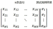
A program spectrum-based defect localization method (SFL) utilizes program coverage information and test case results to build a defect localization model and calculate a suspicious value of each executable statement in a program as a defect statement. SFL defines an information model called program spectrum, which is the input for calculating the suspicious value of a statement. The program spectrum records the running information and the test case result of the program after the program is executed. Suppose that a program P includes N statements, and the test case set T of the program includes M test cases, at least one of which fails, as shown in fig. 1. X ij1 indicates that test case i executed statement j, X ij0 means that test case i has not executed statement j. The matrix mxn records the execution information of each statement in the test case set T. The error vector e is the test case result. Wherein the element e i1 denotes that test case i is a failed test case, e i0 indicates that test case i is a successful test case. Based on the program spectrum, the SFL defined suspicious value calculation formula comprises four parametersEach of which is anp、anf、aepAnd aefThese four parameters are bound to a specific statement. They represent the number of pass or fail test cases, i.e. a, respectively, that execute or not execute the statementnpNumber of test cases indicating passage of not executing the statement, anfNumber of test cases indicating failure to execute the statement, aepNumber of test cases indicating passage of execution of the sentence, aefIndicating the number of test cases that failed to execute the statement. In practice, we expect the true error statement to have a higher aefValue and lower aepValue of when aefMaximum value and aepWhen the minimum value is reached, the statement is not executed by the successful test case, all the failed test cases execute the statement, and the maximum value should be returned when all the suspicious value calculation formulas calculate the suspicious value of the statement. In a typical case, different suspect value calculation formulas may output different suspect values.
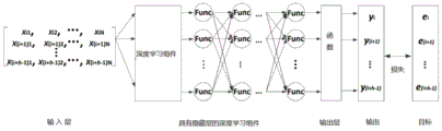
FIG. 2 shows an architecture diagram for defect localization using deep learning techniques. The model includes an input layer, a deep learning component, and an output layer. And in an input layer, the test case coverage information matrix and the test case result vector are used as training samples and corresponding labels. According to the M x N matrix and the corresponding result vector, each time the M x N matrix with h rows is used as the input of the model, the corresponding result vector is used as the label, the ith row is started, at a deep learning component layer, the MLP-FL, the CNN-FL and the BilSTM-FL respectively use a multilayer perceptron, a convolutional neural network and a bidirectional long-and-short-range memory network as deep learning components. At the output layer, SFL uses a sigmoid function (the sigmoid function can output the input data as a value between 0 and 1). The value in the result vector e is different from the value in the sigmoid function output result vector y. And then, parameters of the optimization model are continuously updated by repeatedly iterative training by using a BP algorithm, so that the difference value between a training result vector e and a result vector y is continuously reduced. Despite SFL acquisitionA good positioning effect is achieved, but it still has certain limitations. Their suspect value calculation model does not use the defect context. A defect context is a set of statements of a program, the statements in the set having direct or indirect data or control dependencies with output statements of a failed test case. In fact, the defect context shows the propagation process and mechanism of the defect in the program, which is very important for understanding the program and locating the defect. Thus, relying only on test case results and test case coverage information without taking into account the complex inherent relationships in the defect context can affect the accuracy of the defect location.
Disclosure of Invention
Aiming at the problems in the prior art, the technical problems to be solved by the invention are as follows: how to accurately locate defects using the defect context.
In order to solve the technical problems, the invention adopts the following technical scheme: a defect positioning method based on context sensing comprises the following steps:
s100, data extraction and preparation, which comprises the following specific steps:
s110, a program containing N sentences is arranged, a test case set T containing M test cases runs the program, the test case set T at least contains one failed test case, and the output of each test case in the test case set T is known;
each test case in the T is handed to a program to be executed, and statement coverage information of each test case in the program is obtained, so that the statement coverage information of the test cases in the program forms an M multiplied by N coverage information matrix, and known outputs of all the test cases form a result vector;
s120, constructing a defect context which is a set of statements influencing program errors, determining a statement set from an output statement of a failed test case in the test case set T by using a dynamic slicing technology, wherein the statements in the statement set have a dependency relationship with the selected output statement of the failed test case;
s130: constructing a program statement dependency graph and an adjacency matrix A, and specifically comprising the following steps:
s131: building a program statement dependency graph by adopting a dynamic slicing technology, wherein a node in the program statement dependency graph represents a statement in a defect context, and an edge in the program statement dependency graph represents an association relation between two statements;
the program statement dependency graph is represented as G, G is (V, xi), V represents a set of nodes in the program statement dependency graph, xi represents a set of edges in the program statement dependency graph, and one node ViRepresents a statement in the context of a defect, viE.g. V, a side (V)i,vj) Represents two sentences viAnd vj(v) correlation between themi,vj)∈ξ;
S132: the incidence relation between the nodes on the program statement dependency graph is represented by an adjacency matrix A, wherein AijRepresenting the elements of row i and column j in A, A ij1 indicates that there is a directed edge a between node i and node j pointing from node i to node jij;A ij0 denotes that there is no directed edge between node i and node j that points from node i to node j, aijReflecting whether information flows from node i to node j;
s140: setting a defect context with K sentences, checking N sentences of the program, discarding the sentences not in the defect context to obtain an M multiplied by K matrix, recording the execution information of the K sentences in the defect context in a test case set T, wherein each row of the M multiplied by K matrix represents a test case, y represents a test case, andijthe value of the element in the ith row and the jth column of the M multiplied by K matrix is 0 or1 when y ij1 denotes that the jth statement in the defect context is executed by test case i, y ij0 means not executed;
s200: the specific steps of the model training process are as follows:
s210: embedding node representation vectors into all nodes of the program statement dependency graph through one-hot coding, and initializing the node representation vectors into one-hot representation vectori (1),vectori (1)∈RdThe length of the node representation vector is the number d of the nodes, the superscript (1) represents that the iteration is the first round, and then after t rounds of iteration, each node i fully collects the information of all adjacent nodes so as to obtain the iterative representation m of the nodesi (t),mi (t)∈Rd。
S220: taking the ith row in the M multiplied by K matrix, when the value of the jth column element in the ith row is 1, namely y ij1, the vector j is represented by a node (where vector j is different from the neighbor node vector j, and where vector j represents only the value of j and yijWhere j has the same value) instead of yijWhen the value of the jth column element in the ith row is 0, yijWhen equal to 0, the y is replaced by a zero vectorij;
S230: taking the ith row in the M multiplied by K matrix processed by S220 as the input of the neural network model to obtain an oiValue of oiThe value and the known output e of the test case represented by row iiAnd (3) obtaining a loss value by subtracting the values, and performing iteration on parameters and node vector vectors of the neural network model by using a back propagation algorithm (back propagation algorithm) according to the loss value1To vectorKAnd (6) updating. Setting specific iteration times S according to empirical values, wherein values of different programs S are different, and executing the next step if the iteration times is less than S, otherwise executing S300;
s231: the method for updating the node representation vector comprises the following steps:
taking the node i as a central node, the neural network a: Rd×Rd->R distributes different weights delta to each neighbor node j according to the importance of the neighbor node j to the central node iijNormalizing the correlation coefficients of all the neighbor nodes by using a softmax function;

wherein a represents a neural network a Rd×Rd->R;
S232: computingInteractive information
 Interaction information for the central node i:

wherein A isijIndicating whether information flows from the node i to the node j, vector or not in the adjacent matrix A of the central node i and the neighbor node jjNode representation vector, N, representing neighbor node jiAll neighbor nodes representing a central node i;
s233: GRU is a gate control loop unit, and when a node representation vector is iterated in the t round, GRU enables a vector of a neighbor node j to be usedj (t-1)And mi (t)New node representation vector with output as node i as inputi (t);

After the node representation vector is updated, returning to S220;
s300: and (3) carrying out defect positioning on the defective target program:
for a given faulty program, we want to find out which statement among the statements contained in the faulty program causes the program fault, and for this reason we get a suspicious value between 0 and 1, the larger the suspicious value, the higher the probability that this statement causes the program fault. We then find the location of the defect in the program.
S310: constructing a defect context for the method of S120 of the defective target program, and constructing a K x K virtual test case set, wherein
K is the number of statements of the defect context, each virtual test case only covers one statement of the defect context, and each line in the KxK set of virtual test cases is one virtual test case;
s320: taking the ith 'row in the K multiplied by K virtual test case set, when the value of the jth' column element in the ith 'row is 1, y'ijIf the value of 1 is 1, y 'is replaced by the node representation vector j'ijWhen the value of the j 'th column element in the ith row is 0, that is, y'ij0, then replace y 'with a zero vector'ij;
S330: taking the ith' row in the KxK virtual test case set processed by the S320 as the input of the trained neural network model to obtain an oi' value, said oi' is a suspect value;
s330: and traversing each line in the K multiplied by K virtual test case set to obtain K suspicious values, wherein the range of the K suspicious values is 0-1, and the larger the value of the suspicious value is, the higher the possibility that the statement influences the target program to make mistakes is.
Preferably, the method for constructing the defect context in S120 specifically includes:
determining a statement set from an output statement of a failed test case in the test case set T by using a dynamic slicing technology, wherein the statement in the statement set has a dependency relation with the selected output statement of the failed test case;
the following slicing criteria were used:
failSC=(outStm,incorrectVar,failEx)
wherein outStm is an output statement, a variable in the statement is incorrectVar, incorrectVar represents an erroneous Var, and failEx is a failed execution path.
Compared with the prior art, the invention has at least the following advantages:
the method of the invention is a neural defect localization based on context-aware to analyze the fault context and bring it into suspicion evaluation to improve the defect localization; the method utilizes program slices to model the defect context, represents the defect context as a program dependency graph, and then constructs a graph neural network to analyze and learn the complex relation between sentences in the defect context; a model is eventually learned that evaluates whether each error statement is suspect. The inventors have performed experiments on 12 actual large procedures and compared the method of the present invention with 10 recent defect localization methods. The results show that the method of the present invention can significantly improve the effectiveness of defect localization, for example, the 4.61%, 20%, 29.23%, 49.23% and 64.62% failures are located at the first 1, first 3, first 5, first 10 and first 10 bits, respectively.
Drawings
FIG. 1 is a statement coverage information matrix for M test cases.
Fig. 2 is a diagram of a suspicion evaluation using a neural network.
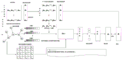
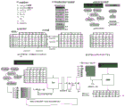
FIG. 3 is a schematic diagram of the method of the present invention.
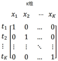
FIG. 4 is a set of virtual test cases.
Fig. 5 is an example of the method of the present invention.
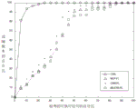
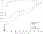
FIGS. 6(a) -6 (d) are comparative EXAM values for CAN and 10 defect localization methods.
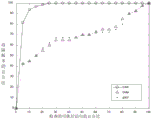
FIGS. 7(a) and 7(b) are CAN and RImp plots.
Detailed Description
The present invention is described in further detail below.
The invention utilizes learning ability to construct a model capable of simulating complex incidence relation in the defect context, thereby achieving the purpose of integrating the error statement context into the defect positioning technology. Therefore, we propose a context-aware defect localization technique, abbreviated as CAN, and it is worth noting that CAN simulates a defect context by building a program dependency graph, which CAN exhibit a set of interacting (data-dependent and control-dependent) statements. The CAN simulates the propagation of the defect in the defect context by utilizing the technology of the neural network, and the defect context is merged into a defect positioning system, so that the position of the defect statement CAN be accurately positioned. Experiments show that in 12 large real programs, the CAN CAN achieve very accurate positioning effect, and 49.23% of defects are positioned in TOP 10. Therefore, the CAN significantly improves the efficiency of the defect localization technology.
Graph Neural Networks (GNNs) can be modeled according to nodes on a graph structure and the incidence relation between the nodes, and through information transfer between the nodes, iterative models are continuously trained, so that convergence of the models can be obtained, and classification or regression problems can be solved. The invention discloses a method for representing a defect context by using a graph structure, which is characterized in that the defect context is represented as data of the graph structure, namely a program dependency graph, the program dependency graph comprises nodes and edges, the nodes are sentences in a program, and the edges are incidence relations among the sentences, including data dependency relations and control dependency relations. The GNNs can learn the element complex association relation in the defect context, so that the defect context is merged into a defect positioning system.
The method utilizes the program dependence graph to model the defect context, utilizes the Graph Neural Networks (GNNs) to analyze and understand the defect context, and further fuses the defect context into a defect positioning system so as to complete the positioning of the program defects. Specifically, the CAN first constructs a defect context by using a program slicing technique, where the context is a directed graph represented by a program dependency graph, nodes in the graph are statements having a direct association with a failure, and edges are associations between the statements. Based on this graph, the CAN uses GNNs to obtain dependencies between statements and then generate corresponding node representation vectors, which are not well represented in conventional defect localization methods (e.g., SFL). The CAN trains by using test cases on the basis of the node representation vectors, so that more accurate statement representation CAN be obtained. Finally, the CAN evaluates each statement as a suspect value of a defective statement using a virtual test case.
Referring to fig. 3, a defect location method based on context sensing includes the following steps:
s100, data extraction and preparation, which comprises the following specific steps:
s110, a program containing N sentences is arranged, a test case set T containing M test cases runs the program, the test case set T at least contains one failed test case, and the output of each test case in the test case set T is known.
And (3) submitting each test case in the T to a program for execution to obtain statement coverage information of each test case in the program, so that the statement coverage information of the test cases in the program forms an M multiplied by N coverage information matrix, and known outputs of all the test cases form a result vector.
Representing the execution information of the program P by using a coverage information matrix and a test case result vector; the CAN uses a graph neural network model to fuse the defect context into a defect positioning system on the basis of a defect program and an information model (covering an information matrix and a test case result vector). The graph neural network model comprises an input layer, a deep learning component and an output layer. And in an input layer, the coverage information matrix of the test case is used as a training sample, and the result vector of the test case is used as a corresponding label. According to the M × N coverage information matrix and the corresponding result vector, each time there are h rows of the M × N coverage information matrix as the input of the model, the corresponding result vector as the label, the initial row is the ith row, i ∈ {1, 1+ h, 1+2h, …, }. At a deep learning component layer, the MLP-FL, the CNN-FL and the BilSTM-FL respectively use a multilayer perceptron, a convolutional neural network and a bidirectional long-and-short-range memory network as deep learning components. At the output layer, the program spectrum based method outputs the input data as a value between 0 and 1 using sigmoid function). The value in the result vector e is different from the value in the sigmoid function output result vector y. And then, continuously updating parameters of the optimization model by repeatedly iterative training by using a BP algorithm (Back propagation algorithm), so that the difference value between a training result vector e and a result vector y is continuously reduced.
S120, constructing a defect context which is a set of statements influencing program errors, and determining a statement set from output statements of a failed test case in the test case set T by using a dynamic slicing technology, wherein the statements in the statement set have a dependency relationship with the selected output statements of the failed test case.
The method for constructing the defect context specifically comprises the following steps:
since the defect context is strongly correlated with a failed execution, statements that directly or indirectly affect the calculation of the erroneous output value of the fault through dynamic data chain/control correlation are included in the defect context, the defect context is constructed using a dynamic slicing method. Determining a statement set from an output statement of a failed test case in the test case set T by using a dynamic slicing technology, wherein the statement in the statement set has a dependency relation with the selected output statement of the failed test case; in particular implementations, such dependencies may be direct or indirect data or control dependencies.
The following slicing criteria were used:
failSC=(outStm,incorrectVar,failEx)
wherein outStm is an output statement, a variable in the statement is incorrectVar, incorrectVar represents an erroneous Var, and failEx is a failed execution path.
It should be noted that: dynamic slicing is one prior art.
Randomly selecting one execution failSC (outStm, incorrectVar, failEx) slicing standard from all failed test cases, thereby obtaining a defect context. After the calculation by using the fail stm (incorrectVar) slicing algorithm, the defect context of the program can be obtained, and then a dependency graph of the program statement is constructed according to the defect context of the program statement.
S130: constructing a program statement dependency graph and an adjacency matrix A, and specifically comprising the following steps:
s131: building a program statement dependency graph by adopting a dynamic slicing technology, wherein a node in the program statement dependency graph represents a statement in a defect context, and an edge in the program statement dependency graph represents an association relation between two statements;
the program statement dependency graph is represented as G, G is (V, xi), V represents a set of nodes in the program statement dependency graph, xi represents the program statement dependency graphDepending on the set of edges in the graph, a node viRepresents a statement in the context of a defect, viE.g. V, a side (V)i,vj) Represents two sentences viAnd vj(v) correlation between themi,vj) E.g. xi; one node in the program statement dependency graph represents one statement in a defect context, edges are incidence relations among the statements and comprise data dependency relations and control dependency relations, failed test cases contain the defect context statements, and therefore relations exist certainly, and nonlinear relations between test case coverage information and test case results are found by means of the neural network and data correlation.
S132: the incidence relation between the nodes on the program statement dependency graph is represented by an adjacency matrix A, wherein AijRepresenting the elements of row i and column j in A, Aij1 indicates that there is a directed edge a between node i and node j pointing from node i to node jij;Aij0 denotes that there is no directed edge between node i and node j that points from node i to node j, aijReflecting whether information flows from node i to node j;
s140: setting a defect context with K sentences, checking N sentences of the program, discarding the sentences not in the defect context to obtain an M multiplied by K matrix, recording the execution information of the K sentences in the defect context in a test case set T, wherein each row of the M multiplied by K matrix represents a test case, y represents a test case, andijthe value of the element in the ith row and the jth column of the M multiplied by K matrix is 0 or1 when y ij1 denotes that the jth statement in the defect context is executed by test case i, y ij0 means not executed;
since the coverage information matrix cannot show the incidence relation between statements and the propagation process of defects in the program, a program statement dependency graph needs to be constructed.
S200: the specific steps of the model training process are as follows:
s210: embedding node representation vectors into all nodes of the program statement dependency graph through one-hot coding, and carrying out one-hot coding on all nodesInitialization of node representation vector to one-hot representation vectori (1),vectori (1)∈RdThe length of the node representation vector is the number d of the nodes, the superscript (1) represents that the iteration is the first round, and then after t rounds of iteration, each node i fully collects the information of all adjacent nodes so as to obtain the iterative representation m of the nodesi (t),mi (t)∈Rd。
S220: taking the ith row in the M multiplied by K matrix, when the value of the jth column element in the ith row is 1, namely y ij1, the vector j is represented by a node (where vector j is different from the neighbor node vector j, and where vector j represents only the value of j and yijWhere j has the same value) instead of yijWhen the value of the jth column element in the ith row is 0, yijWhen equal to 0, the y is replaced by a zero vectorij;
S230: taking the h-th row in the matrix of M multiplied by K after S220 processing as the input of the neural network model to obtain ohValue of oiThe value and the known output e of the test case represented by row hhAnd (3) obtaining a loss value by subtracting the values, and performing iteration on parameters and node vector vectors of the neural network model by using a back propagation algorithm (back propagation algorithm) according to the loss value1To vectorKAnd (6) updating. Setting specific iteration times S according to empirical values, wherein values of different programs S are different, and executing the next step if the iteration times is less than S, otherwise executing S300;
s231: the method for updating the node representation vector comprises the following steps:
taking the node i as a central node, the neural network a: Rd×Rd->R is applied to each neighbor node according to the importance of the neighbor node j to the center node ij assigns different weights δijNormalizing the correlation coefficients of all the neighbor nodes by using a softmax function;

wherein a represents a neural network a Rd×Rd->R;
S232: computing interaction information
 Interaction information for the central node i:

wherein A isijIndicating whether information flows from the node i to the node j, vector or not in the adjacent matrix A of the central node i and the neighbor node jjNode representation vector, N, representing neighbor node jiAll neighbor nodes representing a central node i;
s233: GRU is a gate control loop unit, and when a node representation vector is iterated in the t round, GRU enables a vector of a neighbor node j to be usedj (t-1)And mi (t)New node representation vector with output as node i as inputi (t);

After the node representation vector is updated, returning to S220;
according to the node representation information updating process, the CAN carries out continuous iterative training on the model, and each iteration updates the node representation vector. Suppose the CAN uses the ith row ([ y ] of the information coverage matrix M Ki1,yi2,…,yiK]) And corresponding test case result vector ei. For yijIn other words, y ij1 means node vjTested case TiExecution, CAN will node vjIs represented by vectorjInputting the data into the iteration of the model; y isij0 denotes the node vjCase T not testediExecution, CAN inputs a 0 vector into this iteration of the model.
After the test case T is executediThen, selecting a sentence set strongly related to the defect output and inputting the sentence set into the GNN model, then carrying out iterative training on the node representation vector of the model, and carrying out T during trainingiThe node representation vectors of the non-covered statements remain unchanged, and only the node representation vectors of the covered statements are updated. After the node indicates that the update is completed, the model outputs a value o of 0 to 1 through the linear transformation layeri(i∈{1,2,…,M})。
The CAN continuously iterates each row of the matrix M multiplied by K and the corresponding test case result vector as input, and during iteration, a back propagation algorithm (back propagation algorithm) is used for iterating parameters of the model and the node vector1To vectorKAnd (6) updating. The goal is to continuously narrow the difference between the values in the output o and the test case result vector e. The algorithm continuously calculates from the input layer to the output layer, and then updates the parameters and the node representation in reverse. The CAN trains by adopting a method of dynamically adjusting the learning rate, and the method has two advantages that firstly, the method CAN use a larger learning rate to reduce the loss quickly at the beginning and use a smaller learning rate to prevent the training from missing the optimal point.
In the following formula for calculating LR, one Epoch represents that training data is completely trained once, LR represents the learning rate, DropRate represents the value of each adjustment of the learning rate, and Epoch drop represents the frequency of updating the learning rate. We set the initial learning rate to 0.01 and DropRate to 0.98. The EpochDrap is set according to the size of the test case set.
LR=LR*DropRate(Epoch+1)/EpochDrop
S300: and (3) carrying out defect positioning on the defective target program:
for a given faulty program, we want to find out which statement among the statements contained in the faulty program causes the program fault, and for this reason we get a suspicious value between 0 and 1, the larger the suspicious value, the higher the probability that this statement causes the program fault. We then find the location of the defect in the program.
S310: constructing a defect context for the method of S120 of the defective target program, and constructing a K × K virtual test case set, see fig. 4, where K is the number of statements of the defect context, and each virtual test case only covers one statement of the defect context, so that a total of K test cases, that is, the K × K virtual test case set, is constructed;
each line in the KxK virtual test case set is a virtual test case;
s320: taking the ith 'row in the K multiplied by K virtual test case set, when the value of the jth' column element in the ith 'row is 1, y'ijIf the value of 1 is 1, then the vector j ' is represented by a node (vector j ' here represents only the value of j and y 'ijWherein j has the same value) instead of y'ijWhen the value of the j 'th column element in the ith row is 0, that is, y'ij0, then replace y 'with a zero vector'ij;
S330: taking the ith' row in the KxK virtual test case set processed by the S320 as the input of the trained neural network model to obtain an oi' value, said oi' is a suspect value;
s330: traversing each line in the K multiplied by K virtual test case set to obtain K suspicious values, wherein the range of the K suspicious values is 0-1, and the larger the value of the suspicious value is, the higher the possibility that the statement influences the error of the target program is, that is, the larger the suspicious value is, the more likely the statement is the position of the defect of the program, and the defect is located.
One example of a CAN
FIG. 5 is a diagram showing how CAN CANWorking example, program P in the example contains 8 statements, of which there is a defect statement S4. FIG. 5(a) shows a statement S with a defect4Program P of (1). FIG. 5(b) shows 6 test cases, where T2,T3Is a failed test case. FIG. 5(c) shows the use of test case T by program P3The result of dynamic slicing of (2) includes 6 of the 8 statements. We can see that in the slicing result, S1,S3,S4,S5And S8Influence S8The variable z in (1). Fig. 5(d) shows a diagram representation of the program P, which includes both control dependencies and data dependencies of the program.
Fig. 5(e) shows the CAN training process. The CAN converts the program dependency graph into an adjacency matrix and inputs the adjacency matrix into the GNN model. And then the CNN trains the model by using the coverage information and the test case result vector. In the example, 6 vectors represent a representation of 6 nodes. For example, S1Is a node in the program P, vector1 is S1Is represented by the node(s). Specifically, according to the test case T1=[1,1,1,1,1,1]And its result 0 (the right-most vector of fig. 5 (b)), we input (vector1, vector2, vector3, vector4, vector5, vector6) and 0 in the result vector into the model; according to test case T2=[1,1,1,1,1,1]And its result 1, we input 1 in the (vector1, vector2, vector3, vector4, vector5, vector6) and result vectors after the first iteration into the model; according to test case T3=[1,1,1,1,1,1]And its result 1, we input 1 in the (vector1, vector2, vector3, vector4, vector5, vector6) and result vectors after the previous iteration into the model; according to test case T4=[1,1,1,1,0,1]And its result 0, we input the (vector1, vector2, vector3, vector4, zero vector, vector6) of the previous iteration and 0 in the result vector into the model; according to test case T5=[1,1,1,1,0,1]And its result 0, we input the (vector1, vector2, vector3, vector4, zero vector, vector6) of the previous iteration and 0 in the result vector into the model; according to test case T6=[1,1,1,1,0,1]And its result 0, we will turn the previous roundIterative (vector1, vector2, vector3, vector4, zero vector, vector6) and 0 in the result vector are input into the model. The convergence condition is achieved by continuously training the network repeatedly until the loss is small to some extent. After training, the model reflects the complex nonlinear relationship between the statement representation and the test case coverage information and the test case results.
Finally, the CAN constructs a virtual test case (see fig. 5(f)), which contains 6 test cases, each of which contains only one covered statement. And inputting one virtual test case into the trained model, wherein the output of the model is the suspicious value of the defect statement of the statement covered by the test case set. For example, we set the virtual test case VT1 to [1,0,0,0,0,0]Inputting the input into the trained model, and outputting the output as a sentence S1Is 0.6. Similarly, we can calculate the suspect values for other statements. Since S is not included in the defect context2And S7Thus CAN assigns S2And S7The lowest suspect value is 0. As can be seen from FIG. 5(g), the final list of suspect values is (S)4,S1,S3,S5,S6,S8,S2,S7). True defect statement S4Ranked first.
Experimental testing
A. Construction of the experiment
To verify the validity of CAN, CAN was compared to 10 better defect localization methods. These 10 methods are MLP-FL, CNN-FL, BilSTM-FL, Ochiai, ER5, GP02, GP03, Dstar, GP19 and ER 1', respectively. Further, the experiment used large program objects widely used in the field of defect localization, whose number of code lines varied from 5.4 to 491 kilos.
Table 1 summarizes the characteristics of these subject procedures. For each procedure, the "description" column of table 1 describes the subject procedure; the "version number" column describes the number of defective versions of the program; the "thousand rows" column describes the number of rows of the code; "test case number" describes the number of test cases of a program. The first 4 programs (Chart, m)ath, lang, and time) from Defect4J (b)http://defects4j.org);pythonGzip and libtiff are from ManyBugs (A), (B), (Chttp:// repairbenchmarks.cs.umass.edu/ManyBugs /); space and 4Versions of nanoxml are derived from SIR (C:)http://sir.unl.edu/portal/index.php)。
The experimental environment is as follows: the CPU is I5-2640,64G memory, a 12G NVIDIA TITAN X Pascal GPU and the experimental operating system is Ubantu 16.04.3.
B. Evaluation method
To validate the CAN, we used three widely used evaluation methods: Top-N, EXAM and RImp. Top-N may show the best effect of defect localization, and EXAM and RImp show the overall effect of localization.
TABLE 1 Experimental procedures
| Name of program | Brief description of the drawings | Number of versions | Code line number (thousands of lines) | Number of test cases | |
| python | General- |
8 | 407 | 355 | |
| | Data compression | 5 | 491 | 12 | |
| libtiff | Image processing | 12 | 77 | 78 | |
| space | ADL interpreter | 35 | 6.1 | 13585 | |
| nanoxml_v1 | XML parser | 7 | 5.4 | 206 | |
| nanoxml_v2 | XML parser | 7 | 5.7 | 206 | |
| | XML parser | 10 | 8.4 | 206 | |
| nanoxml_v5 | XML parser | 7 | 8.8 | 206 | |
| chart | JFreeChart | 26 | 96 | 2205 | |
| math | Apache Commons Math | 106 | 85 | 3602 | |
| lang | Apachecommons lang | 65 | 22 | 2245 | |
| time | Joda- |
27 | 53 | 4130 |
Specifically, Top-N shows the positioning accuracy, i.e., how many defect versions in the positioning result of a defect positioning method position the real defect statements in the first N. A higher value of Top-N indicates that more real defect statements are located in the first N bits. Exam is defined as the percentage of statements that have been checked when a true error statement was found. Lower values of Exam indicate better defect localization performance. RImp is defined as the sum of all statements checked for errors that CAN find for all versions of a program divided by the sum of all statements checked for errors that CAN find for all versions of the program using another defect localization method. For CAN, lower rim values represent better positioning performance.
To verify the validity of CAN, CAN was compared to 10 typical defect localization methods. These 10 methods are MLP-FL, CNN-FL, BilSTM-FL, Ochiai, ER5, GP02, GP03, Dstar, GP19 and ER 1', respectively. To evaluate the effectiveness of defect localization, we used three widely used indicators: Top-N accuracy, defect localization accuracy (referred to as EXAM), and relatively improved accuracy (referred to as RImp). Top-N is a metric that shows the effectiveness of the optimal localization of a defect localization method, and EXAM and RImp are two metrics that show the effectiveness of the overall localization. Further, the experiment used large program objects widely used in the field of defect localization, whose number of code lines varied from 5.4 to 491 kilos. We used three widely used evaluation methods: Top-N, EXAM and RImp. Top-N may show the best effect of defect localization, and EXAM and RImp show the overall effect of localization.
Top-N shows the positioning accuracy, i.e. how many defect versions in the positioning result of a defect positioning method position the real defect sentences in the first N. A higher value of Top-N indicates that more real defect statements are located in the first N bits. Exam is defined as the percentage of statements that have been checked when a true error statement was found. Lower values of Exam indicate better defect localization performance. RImp is defined as the sum of all statements checked for errors that CAN find for all versions of a program divided by the sum of all statements checked for errors that CAN find for all versions of the program using another defect localization method. For CAN, lower rim values represent better positioning performance.
Top-N our experiments used Top-N (N ═ 1,3,4,10,20) to compare CAN with 10 superior defect localization methods. Table 2 shows the Top-N distributions of the 11 defect localization methods. In Table 2, CAN achieves optimal performance under all five scenarios of Top-N. Specifically, CAN locates 4.62% of the defective versions to Top-1, 20% of the defective versions to Top-3, 29.23% of the defective versions to Top-5, 49.23% of the defective versions to Top-10, and 64.62% of the defective versions to Top-20.
TABLE 2 Top-N comparison


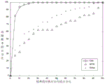
To compare CAN with other defect localization methods, we plot four graphs of the value of EXAM versus the value of fig. 6(a) -6 (d), where the ordinate represents the proportion of the sentences that have been examined in all versions of the defect program and the abscissa represents the percentage of the number of versions of the defect sentence found. One point in fig. 6(a) -6 (d) represents the number of versions of a defect statement that can be checked by checking a certain proportion of executable code as a percentage of the total number of versions. The results of fig. 6(a) -6 (d) show that the CAN curves are much higher than the other 10 defect localization methods. The result shows that the positioning performance of the CAN is obviously superior to other 10 defect positioning methods.
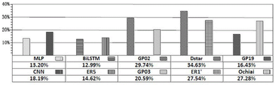
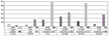
To further validate the experimental results, we used RImp in two scenarios to evaluate CAN. Fig. 7 shows the distribution of RImp in two scenarios: FIG. 7(a) is a RImp comparison plot of RImp over 10 defect localization methods, and FIG. 7(b) is a RImp comparison plot of RImp over 12 experimental subject procedures.
In fig. 7(a), the value of RImp is below 100% in all defect localization methods, which means that CAN is superior to these comparative defect localization methods. The reduction in the total number of statements to be examined ranges from 12.99% for BilSTM-FL to 34.63% for Dstar. This also means that the maximum savings in the number of sentences requiring inspection over other defect localization methods is 87.01% (100% -12.99% ═ 87.01%) of BiLSTM-FL, and the minimum savings in the number of sentences requiring inspection is 65.37% (100% -34.63% ═ 65.37%) of Dstar. This shows that when CAN is compared with other defect locating methods, 65.37% to 87.01% of the number of sentences CAN be saved after all the defect sentences are located.
In fig. 7(b), the RImp value is less than 100% in all the subjects, which means that CAN has a relatively significant improvement in positioning accuracy in all the subjects. The number of statements that need to be examined is reduced from 1.75% of python to 57% of nanoxml _ v 1. This means that the number of sentences to be inspected CAN be reduced on average to 1.75% and 57% compared to the CAN and 10 defect localization methods when locating a defect sentence in all defect versions of python and a defect sentence in all defect versions of nanoxml _ v 1. The maximum saving value of CAN is 98.25% (100% -1.75% ═ 98.25%) in python, and the minimum saving value is 43% (100% -57% ═ 43%) of nanoxml _ v 1. This indicates that the number of sentences to be examined CAN be saved by 43% to 98.25% in all the subjects.
As CAN be seen from the RImp comparison graph, the number of sentences to be inspected is obviously reduced after the CAN is used, which shows that the CAN obviously improves the efficiency of defect location.
To further verify the effectiveness of the present invention, we used Wilcoxon-Signed-Rank for statistical analysis, since RImp only demonstrates specific scale of boost, it is only an overall effect boost demonstration, and some specific details may be missed. Wilcoxon-Signed-Rank Test non-parametric statistics were used to Test the difference between a pair of data, for example, F (x) and G (y), and given a parameter φ, we can use 2-tailed and 1-tailed p-value to obtain a result. For 2-tailed p-value, if p ≧ φ, assume H0: no difference between F (x) and G (y) is accepted; otherwise, suppose H1: differences between F (x) and G (y) are accepted. There are two cases for 1-tailed p-value: 1-tailed (right) and 1-tailed (left), respectively. For 1-tailed (right), if p ≧ φ, then H is assumed0: f (x) and G (y) compare results not accepted by Better; otherwise, suppose H1: f (x) and G (y) compare to result in acceptance of Better. For 1-tailed (left), if p ≧ φ, H is assumed0: f (x) and G (y) compare results not accepted as Worse; otherwise, suppose H1F (x) and G (y) compare to result in Worse being accepted.
In the experiment, the EXAM values of CAN in all defect versions are used as f (x), and the EXAM value of the defect localization method FL1 is g (y). If p <0.05, then assume that the EXAM value for H1 CAN is significantly less than the EXAM value for defect localization method FL1 is accepted. This means that CAN has BETTER positioning performance than FL1, we denote by BETTER. Otherwise, H0: the value of EXAM for CAN is not acceptably smaller than that of defect localization method FL1, which means that CAN is not more efficient than FL1 for localization.
We used Wilcoxon-Signed-Rank Test nonparametric statistics to Test the difference between a pair of data, such as F (x) and G (y), to verify whether CAN improves significantly over other defect localization methods, and we CAN use 2-tailed and 1-tailed p-value to obtain a result given a parameter φ. For 2-tailed p-value, if p ≧ φ, assume H0: no difference between F (x) and G (y) is accepted; otherwise, suppose H1: differences between F (x) and G (y) are accepted. There are two cases for 1-tailed p-value: 1-tailed (right) and 1-tailed (left), respectively. For 1-tailed (right), if p ≧ φ, then H is assumed0: f (x) and G (y) compare results not accepted by Better; otherwise, suppose H1: f (x) and G (y) compare to result in acceptance of Better. For 1-tailed (left), if p ≧ φ, H is assumed0: f (x) and G (y) compare results not accepted as Worse; otherwise, suppose H1F (x) and G (y) compare to result in Worse being accepted. Specifically, the value of EXAM of CAN in all defect versions is used as f (x), and the value of EXAM of the defect location method FL1 is g (y). If p is<0.05, it is assumed that H1, the EXAM value of CAN is significantly less than the EXAM value of defect localization method FL1 is accepted. This means that CAN has BETTER positioning performance than FL1, we denote by BETTER. Otherwise, H0: the value of EXAM for CAN is not acceptably smaller than that of defect localization method FL1, which means that CAN is not more efficient than FL1 for localization.
Table 3 shows that the results of Wilcoxon-Signed-Rank Test non-parameter statistics show that the EXAM value of most of the results of CAN is obviously smaller than that of other defect positioning methods. For A-test, the further the deviation of the A statistic from 0.5 for both comparison methods indicates the greater the difference between the two comparison methods. A-test values greater than 0.64 or less than 0.36 are "medium" differences, and A-test values greater than 0.71 or less than 0.29 are "large" differences. Table 3 shows that CAN is mostly a "large" difference. Therefore, the positioning efficiency of the CAN is higher than that of other defect positioning methods.
TABLE 3 statistical analysis of CAN and 10 Defect localization methods

Therefore, based on the above experimental results and analysis, we CAN conclude that CAN significantly enhances the efficacy of defect localization, and indicate that the neural network has great potential in understanding the defect context and enhancing the efficacy of defect localization.
Finally, the above embodiments are only for illustrating the technical solutions of the present invention and not for limiting, although the present invention has been described in detail with reference to the preferred embodiments, it should be understood by those skilled in the art that modifications or equivalent substitutions may be made to the technical solutions of the present invention without departing from the spirit and scope of the technical solutions of the present invention, and all of them should be covered in the claims of the present invention.
Claims (2)
1. A defect positioning method based on context sensing is characterized by comprising the following steps:
s100, data extraction and preparation, which comprises the following specific steps:
s110, a program containing N sentences is arranged, a test case set T containing M test cases runs the program, the test case set T at least contains one failed test case, and the output of each test case in the test case set T is known;
each test case in the T is handed to a program to be executed, and statement coverage information of each test case in the program is obtained, so that the statement coverage information of the test cases in the program forms an M multiplied by N coverage information matrix, and known outputs of all the test cases form a result vector;
s120, constructing a defect context which is a set of statements influencing program errors, determining a statement set from an output statement of a failed test case in the test case set T by using a dynamic slicing technology, wherein the statements in the statement set have a dependency relationship with the selected output statement of the failed test case;
s130: constructing a program statement dependency graph and an adjacency matrix A, and specifically comprising the following steps:
s131: building a program statement dependency graph by adopting a dynamic slicing technology, wherein a node in the program statement dependency graph represents a statement in a defect context, and an edge in the program statement dependency graph represents an association relation between two statements;
the program statement dependency graph is represented as G, G is (V, xi), V represents a set of nodes in the program statement dependency graph, xi represents a set of edges in the program statement dependency graph, and one node ViRepresents a statement in the context of a defect, viE.g. V, a side (V)i,vj) Represents two sentences viAnd vj(v) correlation between themi,vj)∈ξ;
S132: the incidence relation between the nodes on the program statement dependency graph is represented by an adjacency matrix A, wherein AijRepresenting the elements of row i and column j in A, Aij1 indicates that there is a directed edge a between node i and node j pointing from node i to node jij;Aij0 denotes that there is no directed edge between node i and node j that points from node i to node j, aijReflecting whether information flows from node i to node j;
s140: setting a defect context with K sentences, checking N sentences of the program, discarding the sentences not in the defect context to obtain an M multiplied by K matrix, recording the execution information of the K sentences in the defect context in a test case set T, wherein each row of the M multiplied by K matrix represents a test case, y represents a test case, andijthe value of the element in the ith row and the jth column of the M multiplied by K matrix is 0 or1 when yij1 indicates that the jth statement in the defect context is testedExample i execution, yij0 means not executed;
s200: the specific steps of the model training process are as follows:
s210: embedding node representation vectors into all nodes of the program statement dependency graph through one-hot coding, and initializing the node representation vectors into one-hot representation vectori (1),vectori (1)∈RdThe length of the node representation vector is the number d of the nodes, the superscript (1) represents that the iteration is the first round, and then after t rounds of iteration, each node i fully collects the information of all adjacent nodes so as to obtain the iterative representation m of the nodesi (t),mi (t)∈Rd。
S220: taking the ith row in the M multiplied by K matrix, when the value of the jth column element in the ith row is 1, namely yij1, the vector j is represented by a node (where vector j is different from the neighbor node vector j, and where vector j represents only the value of j and yijWhere j has the same value) instead of yijWhen the value of the jth column element in the ith row is 0, yijWhen equal to 0, the y is replaced by a zero vectorij;
S230: taking the ith row in the M multiplied by K matrix processed by S220 as the input of the neural network model to obtain an oiValue of oiThe value and the known output e of the test case represented by row iiThe values are subtracted to obtain a loss value,
during iteration, parameters and node vector of the neural network model are subjected to back propagation algorithm according to loss value1To vectorKUpdating, specifically setting the iteration times according to the empirical value, executing the next step if the iteration times are less than the preset value, and otherwise executing S300;
s231: the method for updating the node representation vector comprises the following steps:
taking the node i as a central node, the neural network a: Rd×Rd->R distributes different weights delta to each neighbor node j according to the importance of the neighbor node j to the central node iijNormalizing all neighbors by using softmax functionCorrelation coefficients of the nodes;

wherein a represents a neural network a Rd×Rd->R;
S232: computing interaction information
 Interaction information for the central node i:

wherein A isijIndicating whether information flows from the node i to the node j, vector or not in the adjacent matrix A of the central node i and the neighbor node jjNode representation vector, N, representing neighbor node jiAll neighbor nodes representing a central node i;
s233: GRU is a gate control loop unit, and when a node representation vector is iterated in the t round, GRU enables a vector of a neighbor node j to be usedj (t-1)And mi (t)New node representation vector with output as node i as inputi (t);

After the node representation vector is updated, returning to S220;
s300: and (3) carrying out defect positioning on the defective target program:
for a given faulty program, we want to find out which statement among the statements contained in the faulty program causes the program fault, and for this reason we get a suspicious value between 0 and 1, the larger the suspicious value, the higher the probability that this statement causes the program fault. We then find the location of the defect in the program.
S310: constructing a defect context for the method of S120 of the defective target program, and constructing a K x K virtual test case set, wherein
K is the number of statements of the defect context, each virtual test case only covers one statement of the defect context, and each line in the KxK set of virtual test cases is one virtual test case;
s320: taking the ith 'row in the K multiplied by K virtual test case set, when the value of the jth' column element in the ith 'row is 1, y'ijIf the value of 1 is 1, y 'is replaced by the node representation vector j'ijWhen the value of the j 'th column element in the ith row is 0, that is, y'ij0, then replace y 'with a zero vector'ij;
S330: taking the ith' row in the KxK virtual test case set processed by the S320 as the input of the trained neural network model to obtain an oi' value, said oi' is a suspect value;
s330: and traversing each line in the K multiplied by K virtual test case set to obtain K suspicious values, wherein the range of the K suspicious values is 0-1, and the larger the value of the suspicious value is, the higher the possibility that the statement influences the target program to make mistakes is.
2. The method of claim 1, wherein the defect location based on context awareness comprises: the method for constructing the defect context in S120 is specifically as follows:
determining a statement set from an output statement of a failed test case in the test case set T by using a dynamic slicing technology, wherein the statement in the statement set has a dependency relation with the selected output statement of the failed test case;
the following slicing criteria were used:
failSC=(outStm,incorrectVar,failEx)
wherein outStm is an output statement, a variable in the statement is incorrectVar, incorrectVar represents an erroneous Var, and failEx is a failed execution path.
Priority Applications (1)
| Application Number | Priority Date | Filing Date | Title |
|---|---|---|---|
| CN202110152656.5A CN112965894B (en) | 2021-02-04 | 2021-02-04 | Defect positioning method based on context awareness |
Applications Claiming Priority (1)
| Application Number | Priority Date | Filing Date | Title |
|---|---|---|---|
| CN202110152656.5A CN112965894B (en) | 2021-02-04 | 2021-02-04 | Defect positioning method based on context awareness |
Publications (2)
| Publication Number | Publication Date |
|---|---|
| CN112965894A true CN112965894A (en) | 2021-06-15 |
| CN112965894B CN112965894B (en) | 2023-07-07 |
Family
ID=76275004
Family Applications (1)
| Application Number | Title | Priority Date | Filing Date |
|---|---|---|---|
| CN202110152656.5A Active CN112965894B (en) | 2021-02-04 | 2021-02-04 | Defect positioning method based on context awareness |
Country Status (1)
| Country | Link |
|---|---|
| CN (1) | CN112965894B (en) |
Cited By (2)
| Publication number | Priority date | Publication date | Assignee | Title |
|---|---|---|---|---|
| CN113791976A (en) * | 2021-09-09 | 2021-12-14 | 南京大学 | Method and device for enhancing defect positioning based on program dependence |
| CN115629995A (en) * | 2022-12-21 | 2023-01-20 | 中南大学 | Software defect positioning method, system and equipment based on multi-dependency LSTM |
Citations (4)
| Publication number | Priority date | Publication date | Assignee | Title |
|---|---|---|---|---|
| CN104572474A (en) * | 2015-01-30 | 2015-04-29 | 南京邮电大学 | Dynamic slicing based lightweight error locating implementation method |
| CN109144882A (en) * | 2018-09-19 | 2019-01-04 | 哈尔滨工业大学 | A kind of software fault positioning method and device based on program invariants |
| CN110515826A (en) * | 2019-07-03 | 2019-11-29 | 杭州电子科技大学 | A kind of software defect positioning method based on number frequency spectrum and neural network algorithm |
| EP3696771A1 (en) * | 2019-02-13 | 2020-08-19 | Robert Bosch GmbH | System for processing an input instance, method, and medium |
-
2021
- 2021-02-04 CN CN202110152656.5A patent/CN112965894B/en active Active
Patent Citations (4)
| Publication number | Priority date | Publication date | Assignee | Title |
|---|---|---|---|---|
| CN104572474A (en) * | 2015-01-30 | 2015-04-29 | 南京邮电大学 | Dynamic slicing based lightweight error locating implementation method |
| CN109144882A (en) * | 2018-09-19 | 2019-01-04 | 哈尔滨工业大学 | A kind of software fault positioning method and device based on program invariants |
| EP3696771A1 (en) * | 2019-02-13 | 2020-08-19 | Robert Bosch GmbH | System for processing an input instance, method, and medium |
| CN110515826A (en) * | 2019-07-03 | 2019-11-29 | 杭州电子科技大学 | A kind of software defect positioning method based on number frequency spectrum and neural network algorithm |
Non-Patent Citations (3)
| Title |
|---|
| YOU LI等: "Toward Location-Enabled IoT (LE-IoT): IoT Positioning Techniques, Error Sources, and Error Mitigation", 《IEEE INTERNET OF THINGS JOURNAL》, pages 4035 * |
| 张卓等: "增强上下文的错误定位技术", 《软件学报》, pages 266 - 281 * |
| 张旭: "基于上下文的错误定位方法研究", 《中国优秀硕士学位论文全文数据库 信息科技辑》, pages 138 - 281 * |
Cited By (3)
| Publication number | Priority date | Publication date | Assignee | Title |
|---|---|---|---|---|
| CN113791976A (en) * | 2021-09-09 | 2021-12-14 | 南京大学 | Method and device for enhancing defect positioning based on program dependence |
| CN113791976B (en) * | 2021-09-09 | 2023-06-20 | 南京大学 | Method and device for enhancing defect positioning based on program dependence |
| CN115629995A (en) * | 2022-12-21 | 2023-01-20 | 中南大学 | Software defect positioning method, system and equipment based on multi-dependency LSTM |
Also Published As
| Publication number | Publication date |
|---|---|
| CN112965894B (en) | 2023-07-07 |
Similar Documents
| Publication | Publication Date | Title |
|---|---|---|
| CN112965894A (en) | Defect positioning method based on context sensing | |
| CN108563555B (en) | Fault change code prediction method based on four-target optimization | |
| US20090217246A1 (en) | Evaluating Software Programming Skills | |
| CN115629998B (en) | Test case screening method based on KMeans clustering and similarity | |
| CN112668809A (en) | Method for establishing autism child rehabilitation effect prediction model and method and system for predicting autism child rehabilitation effect | |
| CN114787831A (en) | Improving accuracy of classification models | |
| CN116668083A (en) | Network traffic anomaly detection method and system | |
| Zhang et al. | Improving fault localization using model-domain synthesized failing test generation | |
| Amorim et al. | A new word embedding approach to evaluate potential fixes for automated program repair | |
| Schelter et al. | Proactively screening machine learning pipelines with arguseyes | |
| CN117472789A (en) | Software defect prediction model construction method and device based on ensemble learning | |
| Heris et al. | Effectiveness of weighted neural network on accuracy of software fault localization | |
| KR20220095949A (en) | Method of multivariate missing value imputation in electronic medical records | |
| CN111880957A (en) | Program error positioning method based on random forest model | |
| CN114780967B (en) | Mining evaluation method based on big data vulnerability mining and AI vulnerability mining system | |
| CN114330650A (en) | Small sample characteristic analysis method and device based on evolutionary element learning model training | |
| CN112685327A (en) | Method for generating failure test case of model domain | |
| CN117561502A (en) | Method and device for determining failure reason | |
| Lv et al. | Probabilistic diagnosis of clustered faults for hypercube-based multiprocessor system | |
| CN113836027B (en) | Method for generating failure test case by using generation type network | |
| CN113569660B (en) | Learning rate optimization algorithm discount coefficient method for hyperspectral image classification | |
| SINGH | Comparing Variable Selection Algorithms On Logistic Regression–A Simulation | |
| Selvi et al. | Fault Prediction for Large Scale Projects Using Deep Learning Techniques | |
| Grover et al. | DeepCuts: Single-Shot Interpretability based Pruning for BERT | |
| Yamate et al. | Hey APR! Integrate Our Fault Localization Skill: Toward Better Automated Program Repair |
Legal Events
| Date | Code | Title | Description |
|---|---|---|---|
| PB01 | Publication | ||
| PB01 | Publication | ||
| SE01 | Entry into force of request for substantive examination | ||
| SE01 | Entry into force of request for substantive examination | ||
| GR01 | Patent grant | ||
| GR01 | Patent grant |