US9216745B2 - Shared control of semi-autonomous vehicles including collision avoidance in multi-agent scenarios - Google Patents
Shared control of semi-autonomous vehicles including collision avoidance in multi-agent scenarios Download PDFInfo
- Publication number
- US9216745B2 US9216745B2 US14/457,291 US201414457291A US9216745B2 US 9216745 B2 US9216745 B2 US 9216745B2 US 201414457291 A US201414457291 A US 201414457291A US 9216745 B2 US9216745 B2 US 9216745B2
- Authority
- US
- United States
- Prior art keywords
- vehicle
- trajectory
- space
- velocity
- constraint
- Prior art date
- Legal status (The legal status is an assumption and is not a legal conclusion. Google has not performed a legal analysis and makes no representation as to the accuracy of the status listed.)
- Active, expires
Links
- 230000033001 locomotion Effects 0.000 claims abstract description 199
- 238000000034 method Methods 0.000 claims abstract description 122
- 238000012545 processing Methods 0.000 claims abstract description 15
- 230000007246 mechanism Effects 0.000 claims abstract description 7
- 238000005457 optimization Methods 0.000 claims description 183
- 230000003068 static effect Effects 0.000 claims description 46
- 230000006870 function Effects 0.000 claims description 25
- 230000004044 response Effects 0.000 claims description 7
- 238000009434 installation Methods 0.000 claims 27
- 230000008447 perception Effects 0.000 claims 2
- 239000003795 chemical substances by application Substances 0.000 description 253
- 238000002474 experimental method Methods 0.000 description 45
- 230000001133 acceleration Effects 0.000 description 21
- 238000005192 partition Methods 0.000 description 21
- 239000013598 vector Substances 0.000 description 17
- 238000013459 approach Methods 0.000 description 14
- 238000004088 simulation Methods 0.000 description 12
- 238000013461 design Methods 0.000 description 10
- 238000009472 formulation Methods 0.000 description 9
- 238000013507 mapping Methods 0.000 description 9
- 239000000203 mixture Substances 0.000 description 9
- 238000012360 testing method Methods 0.000 description 9
- 238000010586 diagram Methods 0.000 description 8
- 230000008859 change Effects 0.000 description 7
- 230000006399 behavior Effects 0.000 description 6
- 239000011159 matrix material Substances 0.000 description 6
- 238000009826 distribution Methods 0.000 description 5
- 238000004891 communication Methods 0.000 description 4
- 230000000295 complement effect Effects 0.000 description 4
- 230000003247 decreasing effect Effects 0.000 description 4
- 238000011156 evaluation Methods 0.000 description 4
- 230000009467 reduction Effects 0.000 description 4
- 238000004458 analytical method Methods 0.000 description 3
- 230000008901 benefit Effects 0.000 description 3
- 230000001934 delay Effects 0.000 description 3
- 230000000694 effects Effects 0.000 description 3
- 230000005484 gravity Effects 0.000 description 3
- 230000004807 localization Effects 0.000 description 3
- 230000008569 process Effects 0.000 description 3
- 230000009466 transformation Effects 0.000 description 3
- 206010001488 Aggression Diseases 0.000 description 2
- 229920000535 Tan II Polymers 0.000 description 2
- 238000013500 data storage Methods 0.000 description 2
- 238000012886 linear function Methods 0.000 description 2
- 238000012887 quadratic function Methods 0.000 description 2
- 238000009877 rendering Methods 0.000 description 2
- 229920006395 saturated elastomer Polymers 0.000 description 2
- 230000001052 transient effect Effects 0.000 description 2
- 235000004443 Ricinus communis Nutrition 0.000 description 1
- 230000009471 action Effects 0.000 description 1
- 230000016571 aggressive behavior Effects 0.000 description 1
- 208000012761 aggressive behavior Diseases 0.000 description 1
- 238000003491 array Methods 0.000 description 1
- 230000003190 augmentative effect Effects 0.000 description 1
- 230000009286 beneficial effect Effects 0.000 description 1
- 230000015572 biosynthetic process Effects 0.000 description 1
- 230000015556 catabolic process Effects 0.000 description 1
- 238000004140 cleaning Methods 0.000 description 1
- 238000010276 construction Methods 0.000 description 1
- 230000001955 cumulated effect Effects 0.000 description 1
- 238000006731 degradation reaction Methods 0.000 description 1
- 238000009795 derivation Methods 0.000 description 1
- 230000003993 interaction Effects 0.000 description 1
- 238000011835 investigation Methods 0.000 description 1
- 230000005055 memory storage Effects 0.000 description 1
- 230000004048 modification Effects 0.000 description 1
- 238000012986 modification Methods 0.000 description 1
- 230000003287 optical effect Effects 0.000 description 1
- 230000010355 oscillation Effects 0.000 description 1
- 230000010363 phase shift Effects 0.000 description 1
- 239000002574 poison Substances 0.000 description 1
- 231100000614 poison Toxicity 0.000 description 1
- 238000005070 sampling Methods 0.000 description 1
- 238000010845 search algorithm Methods 0.000 description 1
- 239000007787 solid Substances 0.000 description 1
- 238000001356 surgical procedure Methods 0.000 description 1
- 230000001131 transforming effect Effects 0.000 description 1
- 230000007704 transition Effects 0.000 description 1
- 238000013519 translation Methods 0.000 description 1
Images


Classifications
-
- G—PHYSICS
- G05—CONTROLLING; REGULATING
- G05D—SYSTEMS FOR CONTROLLING OR REGULATING NON-ELECTRIC VARIABLES
- G05D1/00—Control of position, course or altitude of land, water, air, or space vehicles, e.g. automatic pilot
- G05D1/0011—Control of position, course or altitude of land, water, air, or space vehicles, e.g. automatic pilot associated with a remote control arrangement
- G05D1/0027—Control of position, course or altitude of land, water, air, or space vehicles, e.g. automatic pilot associated with a remote control arrangement involving a plurality of vehicles, e.g. fleet or convoy travelling
-
- B—PERFORMING OPERATIONS; TRANSPORTING
- B60—VEHICLES IN GENERAL
- B60W—CONJOINT CONTROL OF VEHICLE SUB-UNITS OF DIFFERENT TYPE OR DIFFERENT FUNCTION; CONTROL SYSTEMS SPECIALLY ADAPTED FOR HYBRID VEHICLES; ROAD VEHICLE DRIVE CONTROL SYSTEMS FOR PURPOSES NOT RELATED TO THE CONTROL OF A PARTICULAR SUB-UNIT
- B60W50/00—Details of control systems for road vehicle drive control not related to the control of a particular sub-unit, e.g. process diagnostic or vehicle driver interfaces
- B60W50/08—Interaction between the driver and the control system
- B60W50/10—Interpretation of driver requests or demands
-
- B—PERFORMING OPERATIONS; TRANSPORTING
- B60—VEHICLES IN GENERAL
- B60W—CONJOINT CONTROL OF VEHICLE SUB-UNITS OF DIFFERENT TYPE OR DIFFERENT FUNCTION; CONTROL SYSTEMS SPECIALLY ADAPTED FOR HYBRID VEHICLES; ROAD VEHICLE DRIVE CONTROL SYSTEMS FOR PURPOSES NOT RELATED TO THE CONTROL OF A PARTICULAR SUB-UNIT
- B60W30/00—Purposes of road vehicle drive control systems not related to the control of a particular sub-unit, e.g. of systems using conjoint control of vehicle sub-units, or advanced driver assistance systems for ensuring comfort, stability and safety or drive control systems for propelling or retarding the vehicle
- B60W30/08—Active safety systems predicting or avoiding probable or impending collision or attempting to minimise its consequences
-
- G—PHYSICS
- G05—CONTROLLING; REGULATING
- G05D—SYSTEMS FOR CONTROLLING OR REGULATING NON-ELECTRIC VARIABLES
- G05D1/00—Control of position, course or altitude of land, water, air, or space vehicles, e.g. automatic pilot
- G05D1/0011—Control of position, course or altitude of land, water, air, or space vehicles, e.g. automatic pilot associated with a remote control arrangement
-
- G—PHYSICS
- G05—CONTROLLING; REGULATING
- G05D—SYSTEMS FOR CONTROLLING OR REGULATING NON-ELECTRIC VARIABLES
- G05D1/00—Control of position, course or altitude of land, water, air, or space vehicles, e.g. automatic pilot
- G05D1/02—Control of position or course in two dimensions
- G05D1/021—Control of position or course in two dimensions specially adapted to land vehicles
- G05D1/0268—Control of position or course in two dimensions specially adapted to land vehicles using internal positioning means
- G05D1/0274—Control of position or course in two dimensions specially adapted to land vehicles using internal positioning means using mapping information stored in a memory device
-
- G—PHYSICS
- G05—CONTROLLING; REGULATING
- G05D—SYSTEMS FOR CONTROLLING OR REGULATING NON-ELECTRIC VARIABLES
- G05D1/00—Control of position, course or altitude of land, water, air, or space vehicles, e.g. automatic pilot
- G05D1/02—Control of position or course in two dimensions
- G05D1/021—Control of position or course in two dimensions specially adapted to land vehicles
- G05D1/0287—Control of position or course in two dimensions specially adapted to land vehicles involving a plurality of land vehicles, e.g. fleet or convoy travelling
- G05D1/0289—Control of position or course in two dimensions specially adapted to land vehicles involving a plurality of land vehicles, e.g. fleet or convoy travelling with means for avoiding collisions between vehicles
-
- G—PHYSICS
- G08—SIGNALLING
- G08G—TRAFFIC CONTROL SYSTEMS
- G08G1/00—Traffic control systems for road vehicles
- G08G1/09—Arrangements for giving variable traffic instructions
- G08G1/0962—Arrangements for giving variable traffic instructions having an indicator mounted inside the vehicle, e.g. giving voice messages
- G08G1/0968—Systems involving transmission of navigation instructions to the vehicle
- G08G1/096805—Systems involving transmission of navigation instructions to the vehicle where the transmitted instructions are used to compute a route
- G08G1/096811—Systems involving transmission of navigation instructions to the vehicle where the transmitted instructions are used to compute a route where the route is computed offboard
- G08G1/096816—Systems involving transmission of navigation instructions to the vehicle where the transmitted instructions are used to compute a route where the route is computed offboard where the complete route is transmitted to the vehicle at once
-
- G—PHYSICS
- G08—SIGNALLING
- G08G—TRAFFIC CONTROL SYSTEMS
- G08G1/00—Traffic control systems for road vehicles
- G08G1/09—Arrangements for giving variable traffic instructions
- G08G1/0962—Arrangements for giving variable traffic instructions having an indicator mounted inside the vehicle, e.g. giving voice messages
- G08G1/0968—Systems involving transmission of navigation instructions to the vehicle
- G08G1/096833—Systems involving transmission of navigation instructions to the vehicle where different aspects are considered when computing the route
- G08G1/096838—Systems involving transmission of navigation instructions to the vehicle where different aspects are considered when computing the route where the user preferences are taken into account or the user selects one route out of a plurality
-
- G—PHYSICS
- G08—SIGNALLING
- G08G—TRAFFIC CONTROL SYSTEMS
- G08G1/00—Traffic control systems for road vehicles
- G08G1/22—Platooning, i.e. convoy of communicating vehicles
-
- G—PHYSICS
- G08—SIGNALLING
- G08G—TRAFFIC CONTROL SYSTEMS
- G08G5/00—Traffic control systems for aircraft, e.g. air-traffic control [ATC]
- G08G5/0004—Transmission of traffic-related information to or from an aircraft
- G08G5/0013—Transmission of traffic-related information to or from an aircraft with a ground station
-
- G—PHYSICS
- G08—SIGNALLING
- G08G—TRAFFIC CONTROL SYSTEMS
- G08G5/00—Traffic control systems for aircraft, e.g. air-traffic control [ATC]
- G08G5/0017—Arrangements for implementing traffic-related aircraft activities, e.g. arrangements for generating, displaying, acquiring or managing traffic information
- G08G5/0026—Arrangements for implementing traffic-related aircraft activities, e.g. arrangements for generating, displaying, acquiring or managing traffic information located on the ground
-
- G—PHYSICS
- G08—SIGNALLING
- G08G—TRAFFIC CONTROL SYSTEMS
- G08G5/00—Traffic control systems for aircraft, e.g. air-traffic control [ATC]
- G08G5/0043—Traffic management of multiple aircrafts from the ground
-
- G—PHYSICS
- G08—SIGNALLING
- G08G—TRAFFIC CONTROL SYSTEMS
- G08G5/00—Traffic control systems for aircraft, e.g. air-traffic control [ATC]
- G08G5/0047—Navigation or guidance aids for a single aircraft
- G08G5/0069—Navigation or guidance aids for a single aircraft specially adapted for an unmanned aircraft
-
- G—PHYSICS
- G08—SIGNALLING
- G08G—TRAFFIC CONTROL SYSTEMS
- G08G5/00—Traffic control systems for aircraft, e.g. air-traffic control [ATC]
- G08G5/0073—Surveillance aids
- G08G5/0082—Surveillance aids for monitoring traffic from a ground station
-
- G—PHYSICS
- G08—SIGNALLING
- G08G—TRAFFIC CONTROL SYSTEMS
- G08G5/00—Traffic control systems for aircraft, e.g. air-traffic control [ATC]
- G08G5/04—Anti-collision systems
- G08G5/045—Navigation or guidance aids, e.g. determination of anti-collision manoeuvers
-
- B—PERFORMING OPERATIONS; TRANSPORTING
- B60—VEHICLES IN GENERAL
- B60W—CONJOINT CONTROL OF VEHICLE SUB-UNITS OF DIFFERENT TYPE OR DIFFERENT FUNCTION; CONTROL SYSTEMS SPECIALLY ADAPTED FOR HYBRID VEHICLES; ROAD VEHICLE DRIVE CONTROL SYSTEMS FOR PURPOSES NOT RELATED TO THE CONTROL OF A PARTICULAR SUB-UNIT
- B60W2720/00—Output or target parameters relating to overall vehicle dynamics
Definitions
- the present description relates, in general, to techniques for remotely controlling movements and operations of vehicles such as ground-based vehicles (e.g., a two-to-four or more wheeled vehicle) and aerial vehicles (e.g., a multi-copter, a drone, or the like), and, more particularly, to methods and systems adapted for providing shared control (i.e., both remote and local operator control) over a semi-autonomous vehicle.
- vehicles such as ground-based vehicles (e.g., a two-to-four or more wheeled vehicle) and aerial vehicles (e.g., a multi-copter, a drone, or the like)
- shared control i.e., both remote and local operator control
- an amusement park may provide a ride in which a passenger vehicle is driven along a race track or through an obstacle course, and it may be desirable to allow the passenger to “drive” the vehicle by providing user input indicating a direction they wish to travel and a velocity or speed they want their vehicle to move in the selected direction.
- the vehicle control is preferably shared to provide collision avoidance with static obstacles and also with other vehicles (which may be driven by other ride participants).
- a human operator may remotely control a flying drone such as a multi-copter in a particular air space, but the control is shared with a central controller to avoid collisions or achieve other goals.
- Human-robot shared control has been applied in a variety of settings, but there remains a need for improved shared-control methods that enhance human control such as by providing the human operator more local control or operational freedom while still safely avoiding collisions.
- shared control has been applied in the field of tele-robot operation for tasks including space exploration and surgery.
- methods have been developed for human interaction with a forklift, and shared control has been used with a formation of aerial vehicles via a haptic device.
- Work has also progressed for human-robot shared control with semi-autonomous vehicles such as wheelchairs or similar vehicles and with self-driving cars and other urban transporters.
- the present description provides a shared control method (and relative system for implementing this control method) for a vehicle (e.g., any wheeled or terrestrial vehicle, any aerial vehicle, and the like).
- a vehicle e.g., any wheeled or terrestrial vehicle, any aerial vehicle, and the like.
- a human driver who may be in the vehicle or remote to the vehicle, commands (i.e., provides user input to provide) a preferred velocity.
- the method involves transforming this user input into a collision-free local motion that respects actuator constraints (e.g., vehicle kinematics) and allows for smooth and safe control. Collision-free local motions are achieved with an extension of velocity obstacles that takes into account dynamic constraints and also a grid-based map representation of the space through which the vehicle is traveling under share controlled.
- actuator constraints e.g., vehicle kinematics
- a global guidance trajectory (or “ghost vehicle”) can be used in the shared control method.
- the global guidance trajectory may specify the areas (or volumes) where the vehicle is allowed to drive or move in each time instance.
- schedules are imposed along with or as part of the global guidance trajectory to ensure the vehicles, even under human control, achieve broadly stated goals of reaching particular places (move from a first or start position or location to a second or finish position or location) under predefined time schedules.
- the low computational complexity of the method makes it well suited for multi-agent settings and high update rates, and a centralized function and a distributed function (or centralized and distributed algorithms) are described herein that allow for real-time, concurrent control of many vehicles (e.g., several to 10 to 40 or more vehicles). Extensive experiments have been performed, and the results of these experiments (using a motorized, robotic wheelchair as the vehicle) at relatively high speeds in tight dynamic scenarios are presented in the following description.
- the shared control method includes receiving user input related to a velocity (e.g., speed and direction) for the vehicle within the space.
- the method then includes processing the user input with a local motion planner selectively adjusting the velocity and the direction based on a set of predefined constraints (and the presence of neighboring or other vehicles within the space) to generate a trajectory (which may also be considered a velocity as it defines speed and direction) for the vehicle in the space.
- the method further includes communicating motion control signals including the trajectory to the vehicle and then operating drive mechanisms in the vehicle based on the motion control signals to move the vehicle from a first position to a second position within the space during an upcoming time period.
- the trajectory defines a preferred speed for the vehicle and a direction for movement in the space.
- the set of predefined constraints may include a grid map (e.g., image) of the space that defines locations of obstacles in the space (physical objects such as walls and also, in some cases, virtual objects that may be projected into the space or be displayed on a monitor/display device in the vehicle).
- a grid map e.g., image
- obstacles in the space physical objects such as walls and also, in some cases, virtual objects that may be projected into the space or be displayed on a monitor/display device in the vehicle.
- the processing of the user input includes searching the grid map (e.g., with the vehicle's current position in the space) to identify the obstacles and to define a path
- the set of predefined constraints includes a guidance trajectory defining a passageway through the space that can be traveled by the vehicle without collision with the obstacles, and the trajectory is defined so as to control movement of the vehicle to retain the vehicle within the passageway.
- the passageway may include a set of interconnected waypoints in the space and an active area in which the vehicle may move is associated with each of the waypoints. At least some of the active areas differ in size or shape defining differing areas in which the vehicle may move within the space.
- the set of predefined constraints includes kinematic data for the vehicle
- the processing based on neighboring vehicles in the space includes processing data for collision avoidance for other vehicles moving in the space, velocity predictions for ones of the other vehicles neighboring the vehicle in the space, and/or predictions of movements of the other vehicles during an upcoming time period.
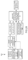
- FIG. 1 is a functional block diagram of a shared control system for semi-autonomous vehicles as described herein;
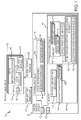
- FIG. 2 illustrates a graph of a wheelchair used as the semi-autonomous vehicle in several experiments implementing a shared control system such as that shown in FIG. 1 ;
- FIG. 3 illustrates a flow diagram of a method of generating a guidance trajectories in a grid map of a drive space for vehicles
- FIG. 4 illustrates a roadmap or grid map with guidance trajectories defined by a combination of interconnected waypoints and their associated active areas
- FIG. 5 illustrates a graph showing use of the shared control method to control movement of a semi-autonomous vehicle within a drive space relative to an obstacle to avoid collision
- FIG. 6 illustrates a graph showing implementation of an avoidance constraint to avoid collision between two neighboring vehicles
- FIG. 7 illustrates a graph showing implementation of a dynamic restriction constraint as part of local motion planning for a vehicle under shared control
- FIGS. 8A-8F illustrate graphs of two representative examples of distributed collision avoidance
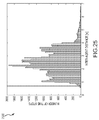
- FIGS. 9A-9D illustrate histographs generated based on the shared control experimental results
- FIGS. 10A and 10B illustrate histograms of computational times for a collision avoidance algorithm for the distributed and centralized cases
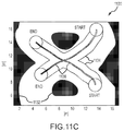
- FIGS. 11A-11C are graphs of vehicles followings two guidance trajectories
- FIGS. 12A and 12B show histograms of distance from a vehicle to a guidance trajectory
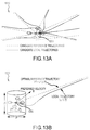
- FIGS. 13A and 13B illustrate graphically schemas of local motion planning showing candidate local trajectories in relation to candidate reference trajectories and showing an exemplary local trajectory
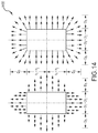
- FIG. 14 provides a graphic representation of two examples of repulsive velocities that may be used in a formulation of local motion planning
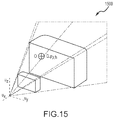
- FIG. 15 provides a graphical representation of an example of a collision avoidance constraint for a static rectangular obstacle showing reference velocities leading to a collision within a given time horizon (note, its complement is non-convex and is linearized);
- FIGS. 16A-16C provide graphical representations of an inter-agent collision avoidance constraint illustrating a velocity obstacle in relative velocity, illustrating projection onto the horizontal plane, and illustrating projection onto a vertical plane, respectively;
- FIG. 17 is a functional block diagram or schema of a controller for use in providing shared control over an aerial vehicle such as a quadrotor helicopter with exemplary variables and frequencies provided;
- FIG. 18 is a graph of a simulation of position exchange for ten quadrotor helicopters using the control methods taught herein;
- FIG. 19 is a set of graphs showing results of an experiment a single quadrotor
- FIG. 20 is a set of graphs showing results of an exchange of two quadrotors in an experiment performed by the inventors
- FIG. 21 is a set of graphs showing results of control experiments using four quadrotor helicopters as the aerial vehicles and using two differing linearization strategies;
- FIG. 22 illustrates a set of graphs showing results of experiments using two quadrotors tracking intersecting trajectories while avoiding collision locally;
- FIG. 23 provides a pair of graphs showing results of experiments using two quadrotors along with a moving human acting as a dynamic obstacle moving through the test fly space;
- FIG. 24 provides graphs showing optimal reference velocity for an experiment, see FIG. 21 , using four quadrotors;
- FIG. 25 illustrates a histogram of distance between all agents accumulated over a plurality of run experiments
- FIG. 26 illustrates distributed and centralized approaches to local motion planning to provide cooperative collision avoidance among decision-making agents
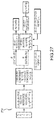
- FIG. 27 illustrates a functional block drawing or data flow diagram showing an example of computation of collision constraints according to the present description.
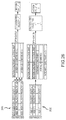
- FIG. 28 illustrates a functional block or data flow diagram showing an example of a distributed non-convex search within convex region.
- methods and systems are described herein that are designed to provide shared control of semi-autonomous vehicles (terrestrial or ground based vehicles and/or aerial vehicles) based, in many cases, on velocity space optimization.
- the method for shared control of a semi-autonomous vehicle is performed based on or using: (1) real-time input from a driver or operator of the vehicle; (2) a guidance trajectory that specifies the areas (which may be 3D spaces or volumes for aerial vehicles) where the vehicle is allowed to drive or move in each time instance; (3) avoidance constraints with respect to other agents (which may be other semi-autonomous vehicles) and/or with respect to a grid map defining the location, size, and shape of static obstacles (real or virtual such as in the form of projected images in the vehicle's drive path/space, images displayed in a vehicle's head's up display, and the like); and (4) motion continuity constraints.
- the local planner may provide local planning of vehicle movements using efficient centralized and/or distributed algorithms based on convex optimization and non-convex search to achieve real-time local planning where an exact grid-based representation of the map can be used in conjunction with a velocity obstacles framework. This may be desirable to allow for real-time control of a larger number of vehicles (e.g., 10 to 40 or more vehicles in a space).
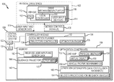
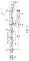
- FIG. 1 illustrates a shared control system 100 for use in controlling movement (velocity, direction, and the like) of semi-autonomous vehicles 110 within a physical drive space 105 .
- the physical drive space 105 may be areas of an amusement park ride where it is acceptable for an operator of one of the vehicles 110 to drive or the space 105 may be a volume of air space through which the vehicles 110 may fly when controlled (e.g., remotely in the case of a drone or multi-copter).
- the driver/operator (not shown) may be seated in or supported on the vehicle 110 or may be at a remote location (e.g., user input 114 may be a remote device communicating velocity inputs via wireless communications).
- the vehicle 110 may include a processor 112 running a local controller 116 that controls operations of a drive mechanism(s)/actuator 118 to cause the vehicle 110 to move in a particular direction and velocity within the space 105 .
- This control may be based on motion control signals 138 from a central control system 130 and also based on input from user input devices 114 .
- a driver/operator 114 may move a steering wheel and accelerator pad to cause the local controller 116 to operate the drive mechanism/actuator 118 within an active area defined/allowed by the motion control signal 138 from central control system to avoid collision and to follow a schedule as the vehicle 110 moves along a guidance trajectory 144 .
- the user input device 114 may also take the form of a joystick that can be manipulated by the driver/operator of vehicle 110 .
- the local controller 116 and/or other components on the vehicle 110 may operate to transmit (wirelessly in most cases) user input data 119 in response to operations of the user input device(s) 114 by the driver/operator, and the user input data 119 typically will include a user-preferred velocity (e.g., direction and speed for the vehicle 110 in drive space 105 ).
- the communicated data 119 may also include sensor or tracking system data that is useful for determining the present location of other/neighbor vehicles 110 in the space and, in some cases, their present velocity, both of which can be used by the control system 120 in controlling the vehicle 110 via motion control signals 138 to avoid collisions among the vehicles 110 in the space 105 .
- the system 100 further includes a central control system 120 that may take the form of a computer or computer-based system specially configured to control the vehicles 110 via motion control signals 138 .
- the control system 120 includes one or more processors 122 managing operations of input/output (I/O) devices such as a monitor, a keyboard, a mouse, a touchpad, a touchscreen, and the like for receiving input from an operator and for displaying data (such as displaying present locations of vehicles 110 in space 105 and the like).
- the processor 122 also runs or executes code in a computer readable medium to provide a controller module 130 , which provides all or a large portion of the shared motion control described herein.
- the controller module 130 may include a local motion planner 132 to generate the motion control signals 138 , and, to this end, the local motion planner 132 may include a trajectory controller 134 along with an optimization engine 136 whose functions and design are described in detail below.
- the processor 122 manages one or data storages devices or memory 140 to store (at least temporarily) data used by the controller module 130 to provide the shared control of the vehicles 110 .
- the memory 140 may be used to store received user input and sensor data 142 from the vehicle 110 .
- the memory 140 may store a guidance trajectory 144 defined by the controller module 130 for controlling the vehicle 110 including defining active areas 145 within the drive space 105 in which the vehicle 110 may be driven by an operator/driver while following a ride path or other planned trajectory.
- the memory 140 also stores a number of optimization constraints 150 that are used by the optimization engine 136 .
- the constraints 150 may include a grid map 152 that maps physical obstacles 154 and, in some embodiments, virtual objects 156 (e.g., displayed 2D or 3D images of objects projected into space 105 or displayed to within or nearby the vehicle 110 to appear to be in the space 105 ) to locations or positions within the drive space 105 .
- the controller module 130 may search the grid map 152 based on a present location of the vehicle 110 to generate a motion control signal 138 that avoids collision with obstacles.
- the memory 140 may be used to store vehicle properties and/or kinematics 158 for the vehicle 110 that can be used to determine the motion control signal 138 (e.g., an acceptable local trajectory for a next control cycle or at a present time).
- Other constraints 150 may include data on other vehicles/agents 160 that may be used to avoid collisions and may be determined from sensor data 119 from the vehicle 110 or from an external tracking system (not shown) operating to determine present locations of each of the vehicles 110 in the drive space 105 .
- the optimization constraints 150 may include velocity predictions 164 for other or neighbor vehicles 110 that may be nearby to the vehicle 110 (“ego vehicle”) in the drive space 105 . This information can be used by the optimization engine 136 to control the vehicle 110 via signals 138 so as to avoid collisions with other flying or airborne vehicles 110 in the 3D space 105 .
- the driver/operator of the vehicle commands the vehicle through the vehicle's user input devices by specifying a desired velocity.
- a guidance trajectory along with or together with active areas (i.e., areas (or spaces) where the vehicle is allowed to drive (or fly)) can be specified to: (1) guide the motion of the vehicle; (2) limit its movements; (3) guarantee that the vehicle has a certain performance even in the case where the driver does not specify a velocity; and (4) control the throughput of vehicles throughout a drive space or ride area.
- the desired velocity and the guidance trajectory are combined and a local trajectory is computed (which is used to generate motion control signals, e.g., after optimization, for the vehicle's drive mechanism/actuator).
- the set of local trajectories is given by a controller (of sufficient continuity, C 2 , in this description) towards a straight-line reference trajectory at velocity u ⁇ 2 (see FIG. 2 ).
- This provides a low dimensional parameterization (given by u) of the local motions and allows for an efficient optimization in reference velocity space to achieve collision-free motions that respect the dynamic constraints of the vehicle.
- the motion is obtained by computing an optimal reference velocity, u*, such that its associated trajectory is collision free, satisfies the motion and guidance constraints, and minimizes the distance to a preferred velocity, ⁇ .
- the preferred velocity takes into account the driver input, a guidance trajectory, and the neighboring obstacles.
- estimated states are used, but, to simplify the notation, no distinction is made herein between estimated and real states.
- This set can be pre-computed by forward simulation and depends on ⁇ dot over (p) ⁇ k and ⁇ umlaut over (p) ⁇ k .
- a trajectory controller appropriate for the vehicle kinematics can then be formulated.
- kinematics of the vehicle the inventors employed wheelchairs for the semi-autonomous vehicles that can have shared control.
- wheelchair vehicle, in this example
- the unicycle model is used, with p the point in-between both tractor wheels, ⁇ the orientation of the vehicle, and v 1 , v 2 the linear and angular speed of the platform.
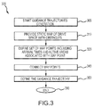
- a method 300 of creating a roadmap or set of guidance trajectories is shown in FIG. 3 .
- the method 300 starts at step 305 such as with selecting a drive area or space in which a vehicle is allowed to move under driver control/input such as with regard to direction and speed.
- the method 300 continues at 310 by providing a static map of the selected drive space that includes locations, shapes, and sizes of obstacles.
- the roadmap may be computed automatically or be created via waypoints connected by straight lines as shown in FIG. 3 . This representation does not require one to account for the dynamics of the vehicle nor to perfectly fit the map since both of these constraints or parameters are considered by the local motion planner.
- a set of waypoints is specified, and, for each waypoint, an arrival time, T l , (or, alternatively, a speed over the segment) and an active area (where the vehicle is allowed to freely move) of a predefined radius, ⁇ l , around the waypoint is provided.
- T l arrival time
- ⁇ l active area
- the method 300 continues with connecting consecutive waypoints.
- the method 300 involves generating or defining the guidance trajectory along with the active area around it (e.g., by interpolation or the like). The method 300 then ends at 390 .
- the vehicle can be assigned to an active area depending on its current position and specified attributes of the guidance trajectories, such as if more than one vehicle can follow that trajectory or if the vehicle must stay in the current one.
- This framework provides an intuitive way to guide a team of vehicles throughout the drive space while giving the vehicles and their drivers/operators limited freedom in their movement via the active areas.
- An active area with a large radius, ⁇ implies greater freedom of movement for the vehicle while an active area with a small radius, ⁇ , imposes less freedom and accurate tracking of the vehicle along and within the guidance trajectory.
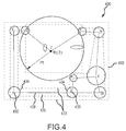
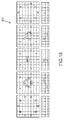
- FIG. 4 illustrates a grid map 400 of a drive space 410 that may be generated with the method 300 of FIG. 3 .
- the drive space 410 includes several rooms and corridors with these available spaces/areas for driving shown at 426 (with lighter or no shading) and occupied spaces or physical/virtual objects shown at 420 (with darker shading).
- nine waypoints, w i are created as shown with exemplary waypoints 430 with arrival times, T i , and a number of different radii, ⁇ i , for their associated active areas 434 .
- the waypoints 430 are connected by straight lines as shown at 438 , and, in between waypoints, the ideal trajectory and active area is given by interpolation.
- waypoints 3 a and 3 b represent a bifurcation and waypoint 7 has a large active area where the vehicles are allowed to freely drive.
- ⁇ i ⁇ 1 ( ⁇ 2 u i joy +u i traj )+(1 ⁇ 1 ) u i A *+u i rep Eq. (6)
- a small hysteresis is introduced to ⁇ 1 and ⁇ 2 to avoid oscillations.
- the input velocity u i joy is proportional to the joystick position (in relative frame of the vehicle).
- the repulsive velocity u i rep is computed with a potential field approach that pushes the vehicle away from both static and dynamic obstacles.
- a linear function weighting the distance to other vehicles is used as follows:
- u i rep Vr ⁇ D _ - d ⁇ ( p i ⁇ ?? ) D _ ⁇ n i , ?? + ⁇ j ⁇ p ij ⁇ D ⁇ Vr ⁇ D - p ij D - r i - r j ⁇ p ij p ij Eq . ⁇ ( 8 )
- V r is the maximum repulsive velocity
- D and D are the maximum distance from which a repulsive force is added
- d(p i ,O) is the distance to the closest static obstacle within the O rj map
- n i,O is the normal vector from it. In order to avoid corner issues, not only the closest point is considered but also an average over the closest points.
- the norm of u i rep is then limited to ⁇ u i rep ⁇ V r .
- u i A * computed from a global path from p i to q i taking into account the map O r but ignoring the kinematic constraints and other vehicles may be added. This term is given by the first control input of a standard A* search in the grid map.
- FIG. 5 illustrates a graph 500 representing implementation of such shared control.
- Components of the preferred reference velocity are shown for a vehicle 510 within the active area 520 of the current point, q, on the ideal trajectory within the drive space.
- An obstacle 530 is shown in the graph with the shared control functioning to avoid collision with the obstacle.
- a local trajectory is given by an optimal reference velocity, u* i , is computed by solving an optimization problem in reference velocity space.
- the optimization problem may be formulated as a combination of a convex optimization with quadratic cost and linear and quadratic constraints and a non-convex optimization.
- the kinematic constraints of the vehicle are included where the vehicle's radius is enlarged by a value ⁇ >0 and the local trajectories are limited to those with a tracking error below ⁇ with respect to the reference trajectory (parameterized by u).
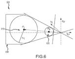
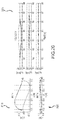
- FIG. 6 illustrates with graph 600 the implementation of the constraint of avoidance of other vehicles or agents.
- This constraint is shown as area 630 for avoidance between two vehicles 610 and 620 , and vehicle avoidance constraint is approximated by three linear constraints as shown in the graph 600 .
- This constraint can then be computed if the distance between the two agents is below a threshold (p ij ⁇ K d ).
- the non-convex constraint 2 ⁇ VO ij ⁇ is approximated by three linear constraints of the form n ij l ⁇ u ij ⁇ b ij l as:
- the linearization of 2 ⁇ VO ij ⁇ is obtained by selecting the linear constraint with maximum constraint satisfaction for the current relative velocity (min l (n ij l v ij ⁇ b ij l )).
- Other sensible choices include linearization with respect to the preferred velocity ⁇ ij or fixed avoidance side (right/left).
- this linear constraint is added to the centralized optimization. For j>m (dynamic obstacles) or when distributed, it can be rewritten as follows.
- n ij l ⁇ u ij n ij l ⁇ ⁇ ( u i - ( 1 - ⁇ ) ⁇ v i - ⁇ ⁇ ⁇ v i ) ⁇ b ij l Eq . ⁇ ( 12 )
- Constraint 2 With regard to a second constraint (“Constraint 2”) concerning active areas, this constraint guarantees that the agent locally remains within the active area.
- the constraint is given by ⁇ p i ⁇ q i +(u i + ⁇ dot over (q) ⁇ i ) ⁇ 2 ⁇ p i 2 with q i being the point on the guidance trajectory for the current time, ⁇ dot over (q) ⁇ i being speed, and ⁇ i the radius of its associated active area (by interpolation between the previous and next waypoint).
- q i the point on the guidance trajectory for the current time
- ⁇ dot over (q) ⁇ i being speed
- ⁇ i the radius of its associated active area (by interpolation between the previous and next waypoint).
- Constraint 3 With regard to a third constraint (“Constraint 3”) concerning avoidance of static obstacles, for agent i ⁇ m, the constraint is given by the reference velocities such that the new positions are not in collision with the enlarged obstacle map, p i +u i t ⁇ O r i + ⁇ i , for all t ⁇ [0, ⁇ ].
- This constraint is kept in its grid-based form (obstacles in FIG. 3 ) to allow the vehicle full navigation capability including being able to move close to the static obstacles and to go inside and/or through small openings.
- the enlarged map, O r i + ⁇ i can be precomputed for several values of ⁇ i .
- each agent should remain within ⁇ i of its reference trajectory.
- ⁇ i [p i , ⁇ dot over (p) ⁇ i , ⁇ umlaut over (p) ⁇ i ]
- the set of reachable reference velocities, R i depends on ⁇ dot over (p) ⁇ i , ⁇ umlaut over (p) ⁇ i , and ⁇ i .
- a mapping, ⁇ , from initial state, ⁇ dot over (p) ⁇ , ⁇ umlaut over (p) ⁇ , and the reference velocity, u, to a maximum tracking error is precomputed and stored in a look up table as:
- ⁇ ⁇ ( u , p . , p ⁇ ) max t > 0 ⁇ ⁇ ( p + tu ) - f ⁇ ( z , u , t ) ⁇ Eq . ⁇ ( 15 )
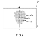
- FIG. 7 illustrates with graph or plot 700 the implementation of the dynamic restrictions constrain with a trajectory controller.
- a vehicle may have a current velocity as shown at 710 , and the areas 720 and 730 represent reachable reference velocities, R i , for the representative current velocity 710 .
- the plot/graph 700 is in reference velocity space aligned with the vehicle axis (e.g., tangential/normal), with forward velocities being displayed.
- the optimization includes two types of constraints: (1) convex (linear and quadratic) and non-convex (grid-based).
- convex linear and quadratic
- grid-based non-convex
- the optimization is divided into two parts. First, a convex subproblem is solved resulting in u i c , and, second, a search within the grid-based constraints is performed that is restricted to the convex area defined by the linear and quadratic constraints.
- the set of convex constraints (Constraints 1 and 2 and bounding box of Constraint 4) is denoted by C.
- Input distributed z 1 , ⁇ 1 and r 1 + ⁇ 1 ; p j , ⁇ dot over (p) ⁇ j and r j ⁇ j neighbor of 1.
- ⁇ j ⁇ 1 .
- u 1:N * [u 1 *, ..., u N *]
- Compute constraints See Eq.
- the complexity of the algorithm can be kept linear with the number of agents, although the centralized is of higher cost.
- the optimization is made up of two variables, one quadratic constraint, four linear constraints (bounding box of Constraint 5), a maximum of m linear constraints of Type 1 (in practice limited to a constant K c ) and a wave expansion within the 2D grid.
- the optimization is made up of 2n variables, n quadratic constraints, less than
- the optimization can be unfeasible due to several causes.
- Fourth, optimization may be unfeasible due to the limited local planning horizon together with over simplification of motion capabilities by reducing them to the set of local motions.
- Fifth, if distributed, unfeasibility may be caused given the use of pair-wise partitions of velocity space with either the assumption of equal effort in the avoidance or constant speed.
- not all world constraints are taken into account for the neighboring agents/vehicles.
- a vehicle may have conflicting partitions with respect to different neighbors, static obstacles, and/or kinematics that render optimization unfeasible for this vehicle.
- deadlock-free navigation is achieved in part due to the u A * term in the optimization that drives the vehicle toward its goal position or guidance trajectory.
- deadlocks are still possible although in degenerated situations. Giving priority to those agents/vehicles further in their guidance trajectory can help resolve this situation, though.
- the input from the driver of the vehicle can also act as a deadlock-breaking input.
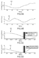
- FIGS. 8A-8F illustrate graphs 810 , 820 , 830 , 840 , 850 , and 860 that show, respectively, examples of robot (or vehicle) and obstacle (or wall) collision avoidance, robot-to-robot (or vehicle-to-vehicle collision avoidance, distance velocity, relative velocity (negative when towards each other and with time-steps where the optimization was unfeasible are marked in gray in the background and where a zero distance indicates that two objects touch), and vehicle position (with the input velocity from the driver being displayed with dashed arrows and the safe vehicle command with solid arrows).
- FIGS. 8A-8F show two representative examples of the distributed collision avoidance, where the driver-commanded velocity, u joy , is shown with arrows in the graphs 850 and 860 .
- safe and smooth velocity between 1 and 2.5 m/s was achieved in very close proximity to a wall when the driver was commanding the vehicle towards the wall. The vehicle slightly slows down as it gets closer to the wall (obstacle).
- a frontal collision with another vehicle is avoided where a relative velocity of about 5 m/s in very close proximity (e.g., below 6 m) with a neighboring vehicle was handled.
- the optimization became unfeasible during 0.15 seconds, which was mostly due to lack of reactiveness in the low level controller and unmodeled dynamics that slowed the vehicle. This renders the algorithm feasible in subsequent time steps.
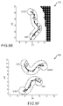
- FIGS. 9A-9D show four histograms 910 , 920 , 930 , and 940 over the shared control experiments Linear and angular velocities are shown with histograms 910 and 920 while histograms 930 and 940 show input velocity from the driver relative to the vehicle. From these histograms, it can be seen that even if the velocity input by the driver seems to follow a bang-bang control of zero (e.g., maximum velocity as seen in histogram 930 of FIG. 9C ), the algorithm adapts the velocity of the vehicle in the range of ⁇ 1 to 3 m/s to remain safe (see, for example, FIG. 9A and histogram 910 ). The driver stops at some times as can be seen from the experiment results.
- a bang-bang control of zero e.g., maximum velocity as seen in histogram 930 of FIG. 9C
- the angular velocity is smooth and within the limits (see, for example, FIG. 9B and histogram 920 ), while the orientation of the desired velocity (see FIG. 9B in vehicle reference frame) is mostly centered in the forward direction and presents clear peaks at 0, +90, and 180 degrees.
- FIGS. 10A and 10B shows histograms 1010 and 1020 (distributed and centralized, respectively) in log scale of the computational time of the collision avoidance algorithm. If no solution is found in 35 ms in this experiment, the algorithm was configured to return unfeasible for that time step.
- FIGS. 10A and 10B show, in log scale to emphasize the infrequent worst cases, statistics of the computational time for the collision avoidance optimization.
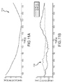
- FIGS. 11A-11C show graphs 1110 , 1120 , and 1130 providing vehicle distance and linear velocities over time (in FIGS. 11A and 11B , respectively) and vehicle position (in FIG. 11C ) with obstacles shown at 1132 , areas covered by vehicle at 1134 , and lines 1136 providing a time indicator.
- FIGS. 12A and 12B show histograms 1210 and 1220 (with and without a driver, respectively) of distance from vehicle to guidance trajectory relative to active area radius.
- FIGS. 12A and 12B show statistics over several experiments of vehicle distance to the guidance trajectory relative to the active area radius.
- the 10 percent offset is due to the proportional tracking controller employed.
- the driver is able to freely move within the active area, but the optimization algorithm successfully constrains the motion of the vehicle so as to avoid collisions with obstacles or other vehicles.
- a method for shared control of a vehicle.
- the driver commands the vehicle by specifying a preferred velocity.
- the specified velocity is then transformed into a local motion that respects the actuator limits of the vehicle and is collision free with respect to other moving vehicles and static obstacles (physical or virtual) given by (or defined by) a grid map of the drive space.
- a global guidance trajectory can be included in some embodiments of the shared control method, and the global guidance trajectory specifies the areas (or spaces) where the vehicle is allowed to drive in each time instance. Good performance has been observed in extensive experimental tests at speeds of up to 3 m/s and in close proximity to other vehicles and obstacles (e.g., walls). Further, the low computational time of the optimization algorithm allows for real-time control of numerous vehicles in the drive space.
- the above description teaches the inventors' shared control for vehicles that are wheeled or driving on the ground in a 2D drive space.
- the inventors further explored application and/or extension of their shared control method (and associated system) to collision avoidance for aerial vehicles especially in multi-agent (or multi-aerial vehicle) scenarios.
- the following paragraphs describe an investigation of local motion planning and collision avoidance for a set of decision-making agents (vehicles) navigating or flying in 3D space.
- the shared control method is applicable to agents that are heterogeneous or homogeneous in size, dynamics, and aggressiveness.
- the method may use and expand upon the concept of velocity obstacles (VO), which characterizes the set of trajectories that lead to a collision between interacting agents.
- VO velocity obstacles
- Motion continuity constraints are satisfied by using a trajectory tracking controller and by constraining the set of available local trajectories in an optimization. Collision-free motion is obtained by selecting a feasible trajectory from the VO's complement, where reciprocity can also be encoded.
- the following three algorithms for local motion planning are presented herein: (1) a centralized convex optimization in which a joint quadratic cost function is minimized subject to linear and quadratic constraints; (2) a distributed convex optimization derived from the centralized convex optimization; and (3) a centralized non-convex optimization with binary variables in which the global optimum can be found but at a higher computational cost.
- the following description also presents results from experiments with up to four vehicles/agents in the form of physical quadrotors (or multi-copters) flying in close proximity and with two quadrotors avoiding a human in the 3D space (or flying space or air space).
- UAVs unmanned aerial vehicles
- multi-rotor helicopters or multi-copters
- Successful navigational control builds on the interconnected competences of localization, mapping, and motion planning and/or control.
- the real-time computation of global collision-free trajectories in a multi-agent setting had proven challenging.
- One approach used was to hierarchically decompose the problem into a global planner, which may omit motion constraints, and a local reactive component that locally modifies the trajectory to incorporate all relevant constraints.
- the local reactive component is one topic of the following paragraphs, and this description teaches a real-time reactive local motion planner that takes into account motion constraints, static obstacles, and other flying vehicles or agents. Further, the important case where other agents/vehicles are themselves decision-making vehicles is addressed with the shared control method (and system).
- a first method is a distributed convex optimization in which a quadratic cost function is minimized subject to linear and quadratic constraints. Only knowledge of relative position, velocity, and size of neighboring agents/vehicles is utilized.
- a second method for local planning uses a centralized convex optimization in which a joint quadratic cost function that is minimized subject to quadratic and linear constraints. This variant scales well with the number of agents and presents real-time capability but may provide, in some cases, a sub-optimal but still useful solution.
- the third method uses a centralized non-convex optimization in which a joint quadratic cost function is minimized subject to linear, quadratic, and non-convex constraints.
- This optimization may be formulated as a mixed integer quadratic program, and this variant explores the entire solution space but can, in some situations, scale poorly with the number of agents/vehicles.
- Each of the optimization methods can: (1) characterize agents as decision making agents that collaborate to achieve collision avoidance; (2) incorporate motion continuity constraints; and (3) handle heterogeneous groups of agents.
- the following description also provides a complexity analysis and a discussion of the advantages and disadvantages of each optimization method.
- the control problem can be thought of as a consideration of a group of n agents freely moving in 3D space.
- n agents freely moving in 3D space.
- p i ⁇ 3 denotes its position
- v i ⁇ dot over (p) ⁇ i its velocity
- a i ⁇ umlaut over (p) ⁇ i its acceleration.
- the goal is to compute for each such agent, at high frequency (e.g., 10 Hz or the like), a local motion that respects the kinematics and dynamic constraints of the ego agent or aerial vehicle.
- the local motion should also be collision free with respect to neighboring agents or aerial vehicles in the 3D space for a short time horizon (e.g., for 2 to 10 or more seconds), which may be thought of as providing local motion that provides collision avoidance.
- a centralized one where a central unit computes local motions for all agents simultaneously
- a distributed one where each agent or vehicle computes independently its local motion.
- no communication between the agents is required, but each agent is able to maintain an estimate of the position and velocity of its neighbors.
- neighboring agents are labeled as dynamic obstacles or decision-making agents, which employ an algorithm that is identical to that in the ego agent or vehicle.
- the local motion planning problem is first formulated as an efficient convex optimization (either centralized or distributed), followed by a non-convex optimization (centralized) that trades off efficiency for richness of the solution space.
- each agent or vehicle is modeled by an enveloping cylinder of radius, r i , and height, 2h i , centered at the agent or vehicle.
- the local motion planning framework is applied to quadrotor helicopters, which are useful in many applications due to their agility and mechanical simplicity. Implementation details, including an appropriate control framework, are described in the coming paragraphs followed by discussion of extensive experimental results using up to four quadrotors along with a human moving through the 3D space.
- FIGS. 13A and 13B illustrate schemas 1310 , 1320 of local motion planning including examples of candidate local trajectories and examples of a local trajectory, respectively, for an agent 1330 (e.g., a quadrotor helicopter).
- agent 1330 e.g., a quadrotor helicopter
- a “global trajectory” is a trajectory between two configurations embedded in a cost field with simplified dynamics and constraints.”
- a “preferred velocity” is an ideal velocity computed by a guidance system to track the global velocity, and it may be denoted as ⁇ 3 .
- a “local trajectory” is the trajectory executed by the agent or vehicle for a short time horizon and is selected from a set of candidate local trajectories.
- a “candidate local trajectory” is one that respects the kinematics and dynamic constraints of the agent or vehicle and is computed from a candidate reference trajectory via a bijective mapping or the like.
- a “candidate reference trajectory” is a trajectory given by a constant velocity, u ⁇ 3 , that indicates the target direction and velocity of the agent or aerial vehicle.
- An “optimal reference trajectory” is a trajectory given by the optimal reference velocity, u* ⁇ 3 , selected from the set of candidate reference velocities and which minimizes the deviation to ⁇ 3 . Further, this trajectory defines the local trajectory.
- One focus of the present description is on local motion planning using a preferred velocity, ⁇ , computed by a guidance or control system in order to track a global trajectory.
- An optimal reference trajectory is computed such that its associated local trajectory is collision free. This provides a parameterization of local motions given by u and allows for an efficient optimization in candidate reference velocity space, 3 , to achieve collision-free motions.
- a collision-free local trajectory (described above and parameterized by u*) is obtained via an optimization in candidate reference velocity space where the deviation to the preferred velocity, ⁇ , is minimized.
- two alternative formulations are presented as a centralized optimization and a distributed optimization, formulated as a convex optimization with quadratic cost and linearized constraints for the following:
- a preferred velocity, ⁇ can be computed given the current position and velocity of the vehicle so as to follow a global plan to achieve either a goal or a trajectory.
- the preferred velocity, ⁇ is given by a trajectory tracking controller for omnidirectional agents.
- the preferred velocity, ⁇ is given by a proportional controller towards the goal position, g i , saturated at the agent's or vehicle's preferred speed, V >0, and decreasing when in the neighborhood as shown in the following:
- u _ i V _ ⁇ min ⁇ ( 1 , ⁇ g i - p i ⁇ K v _ ) ⁇ g i - p i ⁇ g i - p i ⁇ Eq . ⁇ ( 19 )
- K v >0 is the distance to the goal from which the preferred velocity is reduced linearly.
- the preferred velocity, ⁇ is corrected by adding a repulsive velocity, , given by a vector field such as those shown in one of the two examples of repulsive velocities shown in the graph 1400 of FIG. 14 and that pushes agents apart from each other when at a certain distance.
- a repulsive velocity given by a vector field such as those shown in one of the two examples of repulsive velocities shown in the graph 1400 of FIG. 14 and that pushes agents apart from each other when at a certain distance.
- the optimization cost can be given by two parts, with the first one being a regularizing term penalizing changes in reference velocity and the second one being chosen for minimizing the deviation to the preferred velocity, ⁇ i , corrected by the repulsive velocity, i .
- ⁇ i preferred velocity
- penalizing changes in speed leads to a reduction of deadlock situations.
- This idea is formalized as an elliptical cost, higher in the direction parallel to ⁇ i + i , and lower perpendicular to it.
- the set Ri can be precomputed.
- an LQR controller can be used as the function ⁇ (z i ,u i , ⁇ tilde over (t) ⁇ ).
- poison control and local trajectory are decoupled and ⁇ (z i ,u i , ⁇ tilde over (t) ⁇ ) is given by Eq. (40).
- the set Ri would be given by a sphere centered at zero and of radii v max (no continuity in velocity).
- the limits can be obtained from the computed data with:
- ⁇ R i, ⁇ i is then approximated by the largest ellipse (quadratic constraint of the form u i T Q i u i +1 i ⁇ u i ⁇ a i , with Q i ⁇ 3 ⁇ 3 positive semidefinite, l i ⁇ ) fully contained inside ⁇ R i, ⁇ i .
- each agent or vehicle should avoid colliding with static obstacles, other controlled agents or vehicles, and dynamic obstacles.
- a maximum time horizon, ⁇ can be considered for which collision-free motion is guaranteed.
- a static obstacle is given by a region O ⁇ 3 .
- the vehicles or agents are modeled by an enclosing vertical cylinder.
- the disk of radius r centered at c is denoted by D c,r ⁇ 2
- the cylinder of radius r and height 2h centered at c is denoted by C c,r,h ⁇ 3 .
- Constraint 2 a second constraint regarding avoidance of static obstacles can be stated as: for every agent i ⁇ A and neighboring obstacle O, the constraint is given by the reference velocities for which the intersection between O and the agent is empty for all future time instances, i.e., p i +u i ⁇ tilde over (t) ⁇ ⁇ (O ⁇ C 0,r i ,h i ), ⁇ tilde over (t) ⁇ [0, ⁇ ].
- This constraint can be given by a cone in the 3D candidate reference velocity space generated by O ⁇ C 0,r i ,h i ⁇ p i and truncated at (O ⁇ C 0,r i ,hi ⁇ p i )/ ⁇ .
- An example of this constraint for a rectangular object is shown in the fly space or graph 1500 of FIG. 15 .
- Boundary wall constraints are directly added, given by n ⁇ u i ⁇ d(wall,p i )/ ⁇ , with n being the normal vector to the wall and d(wall,p i ) being the distance to it.
- the constraint can be separated in the horizontal plane ⁇ p i H ⁇ p j H +(u i H ⁇ u j H ) ⁇ tilde over (t) ⁇ r i +r j , and the vertical component
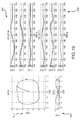
- the constraint is a truncated cone as shown in the graphs 1610 , 1620 , and 1630 of FIGS. 16A-16C (particularly in graph 1610 ), with graph 1610 illustrating a velocity obstacle in relative velocity, graph 1620 illustrating projection onto the horizontal plane, and graph 1630 showing projection onto a vertical plane.
- each collision avoidance constraint can be linearized by selecting one of the five linear constraints.
- the linear constraint chosen may be maximum constraint satisfaction for the current relative velocity:
- a third choice may be maximum constraint satisfaction for the preferred velocity:
- the reference velocity of an agent, j is typically unknown, and only its current velocity, v i , can be inferred.
- a partition should be found such that if both agents select new velocities independently their relative reference velocity, u i ⁇ u j , is collision free.
- the idea of reciprocal avoidance can be followed.
- all agents are considered as independent decision makers solving their independent optimizations.
- an assumption on an agent's, j's, velocity can be made.
- u 1 : m * argmin u 1 : m ⁇ C ⁇ ( u 1 : m ) ⁇ ⁇ s . t . ⁇ ⁇ u i ⁇ ⁇ v max , ⁇ i ⁇ A ⁇ ⁇ quadratic ⁇ ⁇ Constraint ⁇ ⁇ 1 , ⁇ i ⁇ A ⁇ ⁇ linearized ⁇ ⁇ Constraint ⁇ ⁇ ⁇ 2 , ⁇ i ⁇ A ⁇ ⁇ linearized ⁇ ⁇ Constraint ⁇ ⁇ 3 , of ⁇ ⁇ the ⁇ ⁇ form ⁇ ⁇ n i ⁇ j ⁇ ( u i - u j ) ⁇ b ij , ⁇ ⁇ i , j ⁇ A ⁇ ⁇ neighbors Eq . ( 26 ) where the optimization by Eq. (21).
- Algorithm 2 for distributed convex optimization can be states as: each agent, i ⁇ A, independently solves an optimization where its optimal reference velocity, u* i , is computed as:
- u i * arg ⁇ ⁇ min u i ⁇ C ⁇ ( u i ) ⁇ ⁇ s . t . ⁇ ⁇ ⁇ u i ⁇ ⁇ ⁇ v max , ⁇ quadratic ⁇ ⁇ Constraint ⁇ ⁇ 1 , agent ⁇ ⁇ i ⁇ ⁇ ⁇ linearized ⁇ ⁇ Constraint ⁇ ⁇ 2 , agent ⁇ ⁇ i ⁇ ⁇ ⁇ linearized ⁇ ⁇ Constraint ⁇ ⁇ 3 , of ⁇ ⁇ the ⁇ ⁇ from ⁇ ⁇ ⁇ n ij ⁇ u i ⁇ b i , ⁇ j ⁇ A ⁇ ⁇ neighbor ⁇ ⁇ of ⁇ ⁇ i Eq . ⁇ ( 27 ) where the optimization cost is given by Eq. (20).
- a first theoretical guarantee or remark pertains to computational complexity and can be stated as follows: linear in the number of variables and constraints although the centralized is of higher complexity. If distributed, for each agent, the optimization utilizes three variables, one quadratic constrain, and a maximum of m linear constraints for collision avoidance (in practice, limited to a constant value, K c ). If centralized, the optimization uses 3n variables, n quadratic constraints, and less than
- a second theoretical guarantee or remark pertains to safety guarantees and can be stated as: safety is preserved in normal operation. If feasible, collision-free motion is guaranteed for the local trajectory up to a particular time, ⁇ (optimal reference trajectory is collision-free for agents of radii enlarged by the maximum tracking error, ⁇ , and agents stay within ⁇ of it) with the assumption that all interacting agents either continue with their previous velocity or compute a new one following the same algorithm and assumptions.
- a third theoretical guarantee or remark pertains to infeasibility and can be stated as: the optimization can be infeasible due to several causes. First, there may not be enough time to find the solution within the allocated time. Second, there may be differences between the model and the real vehicle. Third, there may be noise in localization and estimation of the agents' states. Fourth, the optimization can be infeasible due to the limited local planning horizon together with an over simplification of motion capabilities by reducing them to the set of local motions. Fifth, if distributed and given the use of pair-wise partitions of velocity, space with either the assumption of equal effort in the avoidance or constant speed, the optimization may be infeasible when not all world constraints are taken into account for the neighboring agents. Thus, an agent may have conflicting partitions with respect to different neighbors rendering its optimization infeasible.
- a fourth theoretical guarantee or remark pertains to deadlock-free guarantees and can be stated as: as for other local methods, deadlocks may still appear. With this in mind, a global planner for guidance may be useful in complex scenarios.
- Algorithm 3 For non-convex optimization (or for centralized mixed-integer optimization) can now be formulated.
- a vector, ⁇ ⁇ T can be defined with (optional) weights for each binary variable, for instance, to give preference to avoidance on one side, and then Algorithm 3 can presented as:
- This optimization can be solved via branch and bound using state of the art solvers.
- the number of variables and constraints can be bounded to be linear with the number of agents, the number of branches to be explored increases exponentially.
- a bound in the resolution time or number of explored branches should be set.
- a distributed MIQP optimization can also be formulated, but collision avoidance guarantees would be lost since this can lead to a disagreement in the avoidance side and reciprocal dances appear.
- FIG. 17 illustrates a control framework or controller 1700 that was implemented to provide control over a quadrotor vehicle 1710 , and, to this end, the controller 1700 includes a number of submodules (e.g., programs executed by a processor of a central unit in a centralized implementation) 1720 - 1790 whose functionality and/or operations are described in the following paragraphs.
- submodules e.g., programs executed by a processor of a central unit in a centralized implementation
- Motion planning may be divided into global planning and local planning.
- global planning in complex environments, a global planner may be desirable for convergence, but in this discussion a fixed trajectory or goal position may be considered or used (as shown at 1720 ).
- the controller 1700 may compute (e.g., with a 10 Hz frequency) a collision-free local motion given a desired global trajectory or a goal position.
- a guidance system 1730 may output a preferred velocity, ⁇ , given a desired global trajectory or a goal position and the current state of the vehicle.
- a collision avoidance module 1740 receives the preferred velocity, ⁇ , and computes the optimal reference velocity, u*, i.e., the closest collision-free candidate reference velocity that satisfies the motion continuity constraints.
- a position controller 1760 controls the position of the quadrotor helicopter (or other aerial vehicle) to the local trajectory and runs at a desired frequency such as 50 Hz offboard in a real-time computer.
- the local trajectory interpreter 1750 receives the optimal reference velocity, u*, at a number of time instances, t k .
- the module 1750 then outputs the control states, q, ⁇ dot over (q) ⁇ , ⁇ umlaut over (q) ⁇ , to satisfy motion continuity at a particular time, and asymptotic convergence to the optimal reference trajectory as may be given by p k +u* ⁇ tilde over (t) ⁇ .
- the position controller 1760 receives setpoints in position, q, velocity, ⁇ dot over (q) ⁇ , and acceleration, ⁇ umlaut over (q) ⁇ , and outputs the desired force, f.
- the vehicle 1710 may be configured to provide a processor, memory, and software to provide a low-level controller that runs onboard (e.g., a 200 Hz or the like) and provides accurate attitude control at high frequency.
- the low-level controller may abstract the nonlinear quadrotor model as a point-mass for the high-level control.
- an attitude controller 1780 that receives a desired force, f (collective thrust and desired orientation) and outputs desired angular rates, w x , w y , w z ; (2) a body angular rate controller that receives the desired body angular rates, and collective thrust, T, and provides an output in the form of a rotation speed setpoint for each of the motors [ ⁇ 1 , . . . , ⁇ 4 ]; and (3) a motor controller that receives the desired rotation speeds of the motors [ ⁇ 1 , . . . , ⁇ 4 ], with some implementations of vehicle 1710 using off-the-shelf motor controllers to interface the four motors of the quadrotor.
- a quadrotor is a highly dynamic vehicle. To account for delays, the state used for local planning may not be the current state of the vehicle but, instead, a predicted one (e.g., as may be provided by forward simulation of the previous local trajectory) at the time when the new local trajectory is sent.
- R B I (R I B ) ⁇ 1 denotes the transformation from the body to the inertial frame
- a point-mass model can be used for the position dynamics.
- the accelerations of the quadrotor's point-mass in the inertial frame, ⁇ umlaut over (p) ⁇ I are given by:
- attitude control an approach may be followed that involves directly converting differences of rotation matrices into body angular rates.
- the desired body angular rates can then be controlled with a standard PD controller and given by:
- w _ f ⁇ ( 1 2 ⁇ ( R _ I B ⁇ R ⁇ B I - R ⁇ I B ⁇ R _ B I ) ) Eq . ⁇ ( 36 ) where ⁇ circumflex over (R) ⁇ ** indicates the estimated rotation matrices.
- FIG. 18 illustrates with graph 1800 position exchange for ten quadrotors in a simulation.
- the top of graph 1800 shows a horizontal (x-y) view and the bottom of graph 1800 shows a vertical (x-z) view.
- Vehicle position is depicted for timestamps 0 s:4 s:6 s:8 s:12 s in an arena of size 8 m by 4 m by 8 m. Convergence to the goal configuration was achieved in about 15 seconds in this simulation. All other results provided herein are for physical quadrotor helicopters.
- the experimental space utilized was a rectangular space that was approximately 5 m by 5.5 m by 2 m in height.
- Quadrotor position was measured by an external motion tracking system running at 250 Hz.
- the control system 1700 was used to control the quadrotors.
- a low-level attitude estimator and controller were run on each quadrotor's IMU, and the quadrotor was abstracted as a point-mass for the position controller.
- the position controller was run on a real-time computer and communication between the real-time computer and the quadrotor was done with a 50 Hz UART bridge.
- the overlying collision avoidance was run in a normal operating system environment and sent a collision-free optimal reference trajectory to the position controller over a communication channel.
- the position controller ensured that the quadrotors stayed on their local trajectories as computed by the collision avoidance algorithm.
- This hard real-time control structure ensured the stability of the overall system and kept the quadrotors on given position references.
- FIG. 19 illustrates with graphs 1910 , 1920 , 1930 , and 1940 a single quadrotor tracking a circular motion given by a sinusoid reference signal in all three position components.
- FIG. 19 shows with graph 1910 the projection of the position p of the quadrotor onto the horizontal plane and shows with graph 1920 the projection onto a vertical plane.
- the reference circular motion is infeasible due to the space limitation of the experiment room, but the local planning successfully avoided colliding with the walls causing the flattened edges in the y component.
- the graph 1930 shows each component of the position p with respect to time as a continuous line, while the point-mass local trajectory q is shown by a dashed line.
- Good tracking performance was observed, although with a small delay due to unmodeled system delays and higher order dynamics.
- a steady-state error is further observed due to the use of an LQR controller without integral part in the experiments.
- Steady-state error is greatest in the vertical component, as a thrust calibration is not performed before flight, and its value varies from quadrotor to quadrotor.
- continuity s imposed in the local trajectory instead of on the real state of the quadrotor. This approach adapts well to poorly calibrated systems, like the one used in the experiments.
- FIG. 19 in graph 1940 shows the measured velocity v of the quadrotor as a continuous line and the velocity of its point-mass local trajectory as a dashed line with respect to time. Good tracking performance was observed, although the delay was more apparent, especially for abrupt changes in velocity, which may be partially due to the unmodeled high-order dynamics of the quadrotor.
- the smoothness of the velocity profile can be adjusted by the parameters w 0 and w 1 in Eq. (40), which can be tuned for overall good performance.
- Position swaps were performed with sets of two and four quadrotors, with about fifty transitions to different goal configurations (both antipodal and random).
- the centralized algorithm (Algorithm 1) and the distributed algorithm (Algorithm 2) were both tested, with the three different linearization options for the collision avoidance constraints described above.
- the joint MIQP optimization (Algorithm 3) was also tested, but it proved too slow for real-time performance at 10 Hz in the experimental implementation. However, in simulation, this approach provided good results.
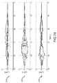
- FIG. 20 shows a representative position exchange for two quadrotors.
- FIG. 20 shows the projection of their paths on the horizontal and vertical planes. The slight change in height is due to the dynamics of the quadrotors.
- FIG. 20 in graph 2030 shows the velocity profile for both quadrotors. The preferred speed of the quadrotors is 2 m/s, and the position exchange takes a few seconds. Very similar performance was obtained in the distributed and centralized cases and with the different linearization options.
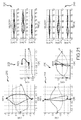
- FIG. 21 with graphs 2110 , 2120 , 2130 , 2140 , 2150 , and 2160 the results these two experiments.
- Graphs 2110 , 2120 , and 2130 illustrate results of use of the first linearization strategy while graphs 2140 , 2150 , and 2160 illustrate results of use of the second linearization strategy.
- Graphs 2110 , 2120 , 2140 , and 2150 show the projection of the position of all quadrotors onto the horizontal plane and a vertical plane.
- Graphs 2130 and 2160 show the velocity profile for all quadrotors.
- the preferred speed was 2 m/s, and the dimensions of the experiment room (fly space) only allowed the quadrotors to fly at a height between 0 and 2 meters.
- the position exchanges were collision free due in part to the local planning algorithm even for this more complex case in which the preferred velocity always points towards the goal positions and, therefore, is not collision free.
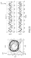
- FIG. 22 illustrates with graphs 2210 , 2220 , and 2230 the results of an experiment in which two quadrotors were tracking intersecting trajectories while avoiding collision locally.
- One quadrotor followed a circular motion (see line 2211 ) and one followed a diagonal motion (see line 2213 such that there are two intersection points in position and time.
- the one following a circular motion finally transitioned to a rest position.
- FIG. 2210 FIG.
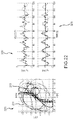
- FIG. 23 with graphs 2310 and 2320 shows the results of control experiments in which two quadrotors were tracking non-colliding circular trajectories with 180 degrees phase shift while a human (see line 2311 ) moved in the arena (test flying space).
- the human was considered as a dynamic obstacle.
- the two quadrotors avoided collisions locally while tracking, as closely as possible, their ideal trajectories.
- Graph 2310 shows the trajectories
- graph 2320 shows the measured velocity for all agents. No collision or deadlock was observed in the experiment, although in some cases a quadrotor had to stop as the optimization became infeasible.
- the human moved at a speed similar to that of the quadrotors ( ⁇ 2 m/s) and was slightly predictable in movements, due to a constant velocity assumption of the experiment.
- Deadlock was not observed in the experiments, but it is possible from a theoretical standpoint and can occur either due to a stop condition being the optimal solution with respect to the optimization objective or due to the optimization problem being infeasible.
- the optimization can be infeasible for two main reasons: (1) for experimental reasons such as the unmodeled high-order dynamics of the vehicle and other uncalibrated parameters such as delays and (2) for reasons inherent in the method (and the trade-off between richness of planning versus low computational time) such as the limited horizon of the local planning or the convexification of the optimization via the linearization of the collision avoidance constraint.
- the local planning optimization which was computed at 10 Hz, was infeasible in under nine percent of the of the cumulated time steps over all experiments (over 40,000 data points at 10 Hz over more than 50 experimental runs).
- the speed of the quadrotor is reduced at a higher than normal rate following Eq. (28), and the quadrotor can, if necessary, be brought to a halt before a collision due to the finite local planning horizon.
- the optimization became feasible after a further one or more time steps, e.g., below 0.5 seconds.
- FIG. 24 illustrates with graphs 2410 , 2420 , and 2430 optimal reference velocity, u*, resulting from the optimization with respect to time for one of the experiments with four quadrotors.
- Six instances in which the optimization is infeasible are observed between the times 65 seconds and 68 seconds. These are points where the optimal reference velocity becomes zero before the quadrotors have converged to their goal positions.
- the effect of these infeasible time steps is to slow down the quadrotors, which in turn has the effect of rendering the local planning feasible in subsequent time steps. This extreme situation was mostly not observed in experiments with only two quadrotors.
- FIG. 25 illustrates a histogram 2500 showing statistics accumulated for the inter-agent distance over the experiments run by the inventors with quadrotor helicopters as the controlled aerial vehicles in a fly space (or 3D space).
- a step decrease in the number of data points with distance below one meter. This is due to the fact that the quadrotors used in the experiment were considered to have a radius of 0.35 meters enlarged by ⁇ 0.1 meters to account for the dynamics, which can decrease towards zero when in close proximity.
- no collision was visually observed and all situations were successfully resolved.
- the quadrotor halted before a collision in a few cases, and this happened, for example, when the velocity estimation is inaccurate or the human moves too fast or with an abrupt change in direction.
- Control systems such as system 100 of FIG. 1
- shared control methods such as the method 300 of FIG. 3
- control systems and methods may apply to collision-free navigation among heterogeneous groups of decision-making agents.
- x denotes scalars, x vectors, M matrices, and X sets.
- the control problem can be stated as a group of n agents freely moving in 2D space for which shared control is required or desired.
- p i ⁇ 3 denotes its position
- v i ⁇ dot over (p) ⁇ i its velocity
- a i ⁇ umlaut over (p) ⁇ i its acceleration.
- the shape of each agent is modeled by an enveloping circle of radius r i , centered at the agent's position p i , and denoted by D(p i ,r i ).
- One goal of the control method is to compute for each agent, at high frequency (e.g., 10 Hz), a local motion that respects the kinematics and dynamic constraints of the ego agent and that is collision free with respect to neighboring agents for a short time horizon (typically, 2 to 5 seconds or the like), and the problem may be labeled simply as “collision avoidance.”
- high frequency e.g. 10 Hz
- a local motion that respects the kinematics and dynamic constraints of the ego agent and that is collision free with respect to neighboring agents for a short time horizon (typically, 2 to 5 seconds or the like)
- collision avoidance typically, 2 to 5 seconds or the like
- This defines the candidate local trajectories given by p( ⁇ tilde over (t) ⁇ ) and a bijective mapping from candidate reference velocities u.
- FIG. 26 illustrates with functional block or data flow diagrams 2610 and 2620 local motion planning according to the present teaching that uses a distributed approach and using a centralized approach, respectively.
- Velocity prediction involves consideration that in each time instance a probability distribution over the future velocities of the ego agent and its neighbors is available or, due to the structure of the problem, it can be relaxed to a utility over the possible future velocities that represents their individual likelihood.
- This distribution can be computed in an environment around the agent's current velocity.
- a value close to 1 indicates that the agent is very likely to choose that reference velocity, while a value close to 0 indicates that it is very unlikely.
- a cost can be defined: Cost, ⁇ i : 2 ⁇ [0, ⁇ ) u i ⁇ i (u i ) Eq. (43) which is then transformed into a utility distribution with a mapping [0, ⁇ ) ⁇ [0,1].
- ⁇ i,aux ( u i ) max(0,1 ⁇ i ( u i )/ K 0 ) Eq. (44) where K 0 is the cut-off cost, and this can be normalized to
- ⁇ i ⁇ ( u i ) ⁇ i , aux ⁇ ( u i ) ⁇ u i ⁇ R 2 ⁇ ⁇ i , aux ⁇ ( u i ) Eq . ⁇ ( 45 )
- three cases are discussed: (1) a simplified prediction; (2) utility computed from a motion prediction; and (3) utility computed from a cost distribution.
- ⁇ j is the preferred velocity of agent j.
- the velocity prediction may be provided using a utility given a motion prediction.
- a utility given a motion prediction.
- GP Gaussian Process
- the velocity prediction may be provided using a utility given by a cost from the environment.
- the environment characteristics can be taken into account when constructing the weights over the reference velocities, u j . This approach then provides information about the maneuverability of the neighboring agents and their motion preferences and can later be incorporated in the local motion planning step.
- the cost, ⁇ j (u j ) can be given by the sum of several terms, which may include the following and should be saturated: (1) deviation from current velocity, where the agent is expected to continue with its current velocity (K 1 ⁇ u j ⁇ v j ⁇ 2 ); (2) deviation from preferred velocity, where velocities close to its preferred velocity incur lower cost (K 2 ⁇ u j ⁇ j ⁇ 2 ); (3) cost to go, determined as being proportional to the distance from the desired goal to the expected position after the time horizon of the local planner and as may be determined with a search algorithm or from a pre-computed distance transform map, and, with K 3 being a design constant, the term can be normalized to [0,K 3 v max ⁇ ] by K 5 max (0, cost2go(p j k +u j ⁇ ) ⁇ C 0 ) Eq.
- Costs 1 and 4 to 6 can be obtained by all agents with common observations.
- costs 2 and 3 are agent specific and cannot be observed, although an estimation may be available and used.
- each agent computes a preferred velocity, ⁇ i , which would be its desired reference velocity in the absence of other agents. It can be obtained to achieve different objectives.
- a first objective may be goal directed.
- the preferred velocity, ⁇ i can be computed from the “cost to the goal” map (e.g., obtained by an F1 expansion as discussed above). Its orientation is that of the shortest path to the goal from the current position of the agent, and its magnitude equals the preferred speed, V >0, of the agent reduced linearly in the neighborhood of the goal.
- a second objective may be trajectory following.
- a third objective may be semi-autonomous driving.
- the preferred velocity, ⁇ i can be specified by a driver, with the preferred velocity, ⁇ i , being proportional to the driving wheel or joystick position (in the relative frame of the vehicle).
- the preferred velocity, ⁇ i often will be corrected with a repulsive velocity, i , that pushes the vehicle away from both static and dynamic obstacles. Collision-free motion is guaranteed by the constraints that are directly included in the local planning framework. Optimal solutions that minimize deviation with respect to the preferred velocity do produce solutions where agents come arbitrarily close to each other. This behavior can be unsafe in some real world scenarios with uncertainties in sensing and kinematic model.
- the repulsive velocity is, thus, included to help maintain a minimum distance to other agents and walls, and it moves the ego-agent (controlled vehicle) away when it is too close.
- a linear function weighting the distance to other vehicles can be used that is adapted to specify the maximum velocity allowed towards the obstacles or other vehicles as shown by:
- u . i u i ⁇ ⁇ o rep ⁇ n i , o + ⁇ j ⁇ ⁇ p ij ⁇ D ⁇ u i ⁇ ⁇ j rep ⁇ p ij p ij Eq . ⁇ ( 48 )
- u i ⁇ ⁇ o rep max ⁇ ( V r ⁇ D _ - d ⁇ ( p i , O ⁇ i ) D _ - V _ , u _ i ⁇ n i , o ) Eq .
- u i ⁇ ⁇ j rep max ⁇ ( V r ⁇ D - p ij D - r i - r j - V _ , u _ i ⁇ p ij p ij ) Eq . ⁇ ( 50 )
- V r is the maximum repulsive velocity
- D and D are the maximum distance from which a repulsive force is added
- d(p i ,O) is the distance to the closest static obstacle within the O r i map
- n i,O is the normal vector from it.
- the super-index, * k is dropped to simplify the notation.
- the set of reachable reference velocities, R i depends on ⁇ dot over (p) ⁇ i , ⁇ umlaut over (p) ⁇ i , and ⁇ i .
- a mapping, ⁇ , from the initial state, ⁇ dot over (p) ⁇ i , ⁇ umlaut over (p) ⁇ i , and a reference velocity, u i , to maximum tracking error is precomputed and stored in a look up table as:
- the local trajectories can be defined by two sections including a circumference arc followed by a straight line path at a constant speed, u i .
- the angular velocity over the arc was, in one model, defined such that the correct orientation was achieved within a fixed time, T, and the linear velocity minimized the tracking error of the reference trajectory.
- a closed form solution was obtained for the set R i , but, in this simple formulation, the robots had no constraints in acceleration and the linear and angular velocities presented a discontinuity.
- this modeling may be applied to car-like robots with bicycle kinematics.
- a trajectory controller can be employed to track the referenced trajectory given by a constant speed, u i , and was obtained by applying full-state linearization via dynamic feedback to the non-linear system. Additional constraints such as maximum steering angle and velocity and linear velocity and acceleration were added as saturation limits. This framework was useful as it guaranteed continuity in both linear velocity and steering angle.
- a point mass v th -order integrator may be used to model the controlled vehicle.
- a controller for point mass v th -order integrator dynamics can and has been described, which is continuous up to the v th derivative of the initial state.
- the robot may be modeled as a unicycle with dynamic constraints.
- a robotic wheelchair may be modeled as a unicycle.
- the relevant variables are shown in FIG. 2 .
- p is not fully controllable.
- Equation (55) defines the local motion of the vehicle's holonomic point. Additional constraints can be added such as maximum linear and angular velocity (
- the vehicle may be modeled as an omnidirectional boat with dynamic constraints.
- the methods taught herein have also been applied to control a team of omnidirectional boats controlled by three rotating propellers.
- An LQR controller in position in velocity was employed to track the reference trajectory. Additional saturation limits were included that accurately model the boat dynamics.
- static obstacles are typically given by a grid map, O 0 , of occupied space.
- O 0 The dilated obstacle map of the positions, p, where a disk, D(p,r), is in collision with a static obstacle is denoted by O r . Its complement defines the positions for which the agent is not in collision.
- a constraint (“Constraint 2” in some of this description) can be stated regarding collision avoidance with static obstacles.
- the constraint can be kept in its original grid-based representation or convexified.
- Grid-based forms can be used due to the mapping between velocities and future positions. This provides a vehicle with full navigation capability including being able to move close to the static obstacles and being able to go inside small openings.
- the enlarged map O r i + ⁇ i can be precomputed for several values of ⁇ i .
- convexification for simplicity and lower computational cost, the static obstacles within a neighborhood of the robot may be approximated by a union of linear constraints forming a convex polygon. This is the case, of example, for a polygon where the closest side is taken as the linear constraint, but, in complex environments, this can be suboptimal.
- the grid-based representation or its convex approximation can be employed.
- pair-wise collision avoidance the constraint for inter-agent avoidance (or avoidance of dynamic obstacles), and it may be based on work on velocity obstacles, reciprocal velocity obstacles, and/or their convex counterpart.
- the constraint is described in its relative velocity space formulation, which can be employed in a centralized optimization. Then, three different approaches to obtain a distributed version are described.
- the inter-agent collision avoidance constraint can be obtained for the reference trajectory following or using work on velocity obstacles.
- the velocity obstacle is formed by the relative reference velocities that lead to a collision between the two agents within the given time horizon ⁇ .
- Constraint 3 or a constraint to provide inter-agent collision avoidance
- control obstacle or C N
- C N -CO considers all interacting agents or robots as linear systems with order N dynamics. After linearization of the C N -CO, the method described herein proceeds analogously.
- non-convex constraint 2 ⁇ VO ij ⁇ (inter-agent collision-free reference velocities) can be approximated by three linear constraints of the form n ij l ⁇ u ij ⁇ b ij l , with l ⁇ 1,2,3 ⁇ and given by:
- Pair-wise collision avoidance may also include avoidance of a velocity obstacle in the distributed case.
- the new reference velocity of the neighboring agent, u j is unknown.
- Pair-wise collision avoidance may further include velocity obstacles (or a distributed reciprocal).
- velocity obstacles or a distributed reciprocal
- One attempt towards taking into account decision making can be considered the work on the reciprocal velocity obstacle, where the velocity obstacle was slightly translated and the assumption was made that both agents share the avoidance effort with a known weight.
- ORCA optimal reciprocal collision avoidance
- the goal with regard to the velocity obstacle is to obtain two sets F i
- agent i can freely select a velocity within F i
- An avoidance topology can be fixed by first linearizing the constraint 2 ⁇ VO ij ⁇ .
- the partition is reduced to obtaining a value b i
- ⁇ u j ⁇ (1 ⁇ i
- Equation (60) the linear constraint is computed from:
- FIG. 27 illustrates with the functional block system or data flow diagram 2700 exemplary computation of collision constraints.
- Reciprocal methods are a first step towards modeling inter-agent decision making, but they consider all agents equal or a known cooperation effort. Velocity predictions and external factors such as static obstacles were not taken into account.
- the following provides a method to incorporate a velocity prediction or utility function over future velocities in the selection of the sets F i
- a cooperation measure is defined as a function of the utility functions ⁇ i (u i ) and ⁇ j (u j ) of both interacting agents and the partition is found such that the cooperation measure is maximized.
- j ) is given by: (1) Y(l) which can favor a certain avoidance topology, for example to encode preferences for avoidance to the right; and (2) Y(i,l,b i
- Y(l) which can favor a certain avoidance topology, for example to encode preferences for avoidance to the right
- j ) which is a function of the utility of the collision-free velocities within the partition F i
- Y ⁇ ( i , l , b i ⁇ ⁇ j ) ⁇ u i ⁇ D i ⁇ F i ⁇ ⁇ j ⁇ ⁇ i ⁇ ( u i ) ⁇ d u i ⁇ u i ⁇ D i ⁇ ⁇ i ⁇ ( u i ) ⁇ d u i Eq . ⁇ ( 63 ) with F i
- j ) Y ( l )+ Y ( i,l,b i
- the min-max value is given by: Y 2 ( l,b i
- j ) Y ( l )+min( Y ( i,l,b i
- j ) is a monotonically increasing/decreasing function of b i
- an optimal reference velocity, u* i is computed by solving an optimization in candidate reference velocity space.
- the preferred velocity, ⁇ i of the ego-agent is given, together with the current position and velocity of neighboring agents.
- the optimization cost which is described in detail below, is denoted by C(u i ) and C(u 1:m ).
- each agent, i independently solves an optimization where its optimal reference velocity, u* i , is computed as follows, with the position p j and velocity v j of neighboring agents being known:
- u i * arg u i min ⁇ C ⁇ ( u i ) s . t . ⁇ ⁇ u i ⁇ ⁇ u max u i ⁇ R i ⁇ ⁇ respects ⁇ ⁇ motion ⁇ ⁇ constraints u i ⁇ ⁇ collision ⁇ - ⁇ free ⁇ ⁇ w . r . t . ⁇ static ⁇ ⁇ obstacles ⁇ u i ⁇ F i
- u 1 : m * arg ⁇ min u 1 : m ⁇ C ⁇ ( u i : m ) s . t . ⁇ ⁇ ⁇ u i ⁇ ⁇ ⁇ u max , ⁇ i ⁇ m u i ⁇ R i ⁇ ⁇ respects ⁇ ⁇ motion ⁇ ⁇ constraints ⁇ ⁇ ⁇ i ⁇ m u i ⁇ ⁇ collision ⁇ - ⁇ free ⁇ ⁇ w . r . t ⁇ ⁇ static ⁇ ⁇ obstacles ⁇ ⁇ ⁇ i ⁇ m u i ⁇ ⁇ collision ⁇ - ⁇ free ⁇ ⁇ w . r t ⁇ ⁇ neighboring ⁇ ⁇ agents ⁇ ⁇ ⁇ i ⁇ m
- j for distributed avoidance are not required or utilized.
- optimization 1 is solved with quadratic cost C(u i ) and linearized constraints. Computational complexity is very low and scalability is very good, but the solution space is greatly reduced due to the linearization of the constraints and the partition of the reference velocity space.
- a centralized, convex optimization may be used to compute the optimal reference velocities. In this case, Optimization 2 is solved with quadratic cost, C(u i:m ), and linearized constraints. Computation complexity is low and scalability is relatively good, but the solution space is partially reduced due to the linearization of the constraints.
- a centralized, non-convex optimization may be utilized.
- Optimization 2 is solved with quadratic cost, C(u i:m ), and non-convex constraints. Computational complexity is high and scalability is poor, but the complete solution space is explored.
- a distributed, non-convex search may be performed within the convex region to compute the optimal reference velocities.
- Optimization 1 is solved with quadratic cost, C(u i:m ), or arbitrary utilities ⁇ i (u i ), linearized inter-agent collision avoidance constraints, non-convex motion constraints, and static obstacle avoidance constraints. Computational complexity is low and stability is good, but the solution space is reduced due to the linearization of the collision-avoidance constraints and the partition of the reference velocity space to guarantee safety in the distributed case.
- the re-parameterization of the trajectories guarantees that the vehicles stop within the time horizon of the local planner, unless the optimization becomes feasible in a later time step.
- C(u i ) is defined by a quadratic function given by two terms. The first one is a regularizing term penalizing changes in velocity, and the second one minimizes the distance to the preferred velocity.
- R i The constraints for avoidance of static obstacles are also linearized, and the set, R i , defining the motion constraints is approximated by a convex polygon (formed by a union of linear constraints). If R i is given by two convex regions, only one is selected such as either the closest one to the previous reference velocity or the closest one to the preferred reference velocity. Note that at high speeds, R i is formed by a single region.
- the set of all linear constraints may be denoted by C lin .
- Optimization 1 may be formulated as a quadratic program with linear constraints as:
- u i * arg ⁇ min u i ⁇ C ⁇ ( u i ) ⁇ ⁇ s . t . ⁇ ⁇ u i ⁇ ⁇ u max ⁇ ⁇ n s ⁇ u i ⁇ b s ⁇ ⁇ s ⁇ C lin Eq . ⁇ ( 71 )
- a collision-avoidance constraint is computed and linearized (e.g., as described above).
- the set of linear constraints for inter-agent collision avoidance (one for each pair of neighboring agents) is denoted by C rel .
- the constraints for avoidance of static obstacles are also linearized and the sets R i are approximated by a convex polygon.
- the set of these linear constraints for agent i is denoted by C i,abs .
- Optimization 2 can be formulated as a quadratic program with linear constraints as:
- u 1 ⁇ : ⁇ m * arg u 1 ⁇ : ⁇ m min ⁇ C ⁇ ( u i ⁇ : ⁇ m ) ⁇ ⁇ s . t . ⁇ ⁇ u i ⁇ ⁇ u max , ⁇ i ⁇ m ⁇ ⁇ n ij ⁇ ( u i - u j ) ⁇ b ij , ⁇ i , j ⁇ ⁇ neighboring ⁇ ⁇ agents ⁇ ⁇ n s ⁇ u i ⁇ b s , ⁇ i ⁇ [ 1 , m ] , ⁇ s ⁇ ?? i , abs Eq . ⁇ 73
- Equation (72) The optimization cost of Equation (72) is kept, with an optional modification. Since an avoidance topology is not defined beforehand, a side preference for the collision avoidance can now be added by appropriately selecting a penalty for the binary variables.
- the vector of linear cost with respect to the binary variables is then given by:
- I 2 is the set of agents whose set R i is approximated by two convex regions
- I 1 [1,m] ⁇ I 2
- Optimization 2 in this case, can then be formulated as a quadratic program with linear constraints as:
- u 1 : m * arg ⁇ min u 1 : m ⁇ b ⁇ ( Cu i : m ) + f ⁇ ⁇ b ⁇ ⁇ s . t . ⁇ ⁇ ⁇ u i ⁇ ⁇ ⁇ u max , ⁇ i ⁇ [ 1 , m ] ⁇ ⁇ n s l ⁇ ( u i - u j ) - ⁇ s l ⁇ M ⁇ b s l , ⁇ s ⁇ ??
- an initial point may be specified.
- the solution of the convex optimization discussed herein may be well suited for this purpose since it typically returns a feasible (although not optimal) solution with very low computational time. Optimality of the solution increases with time as more nodes are explored.
- the algorithm can exit at any time to cope with run-time constraints, and, hence, this method features anytime properties.
- centralized, non-convex optimization may be formulated as message passing optimization.
- this non-convex optimization can be solved using an improved version of the alternating direction method of multipliers (ADMM) algorithm known to those skilled in the art.
- ADMM alternating direction method of multipliers
- a convex cost, C(u i ), is given by Eq. 70.
- the set of convex constraints is formed by the inter-agent linearized collision avoidance constraints (i.e., set F i
- the set of non-convex constraints is formed by the static obstacle collision avoidance constraint and the set R i accounting for the motion constraints and is denoted by ⁇ tilde over (C) ⁇ i .
- Both non-convex constraints are given by grid representations of identical resolution.
- Equation (70) The quadratic cost defined in Equation (70) is maintained, and the algorithm proceeds as follows:
- function feasibleDynamics(u i ) checks in a precomputed grid if the tracking error is below ⁇ i , given the initial state of the vehicle (if u i ⁇ R i then return ‘true’; else ‘false’).
- the function expandNeighbors adds the neighboring grid points if they are within the convex region defined by the convex constraints in and they are not previously explored, with the function defined as:
- variable maximum tracking error, ⁇ i and associated radius enlargement is desirable for feasibility.
- j ⁇ , r i +r j + ⁇ i + ⁇ j ⁇ d(p i ,p j ) should be satisfied, i.e., the extended radii of the robots should not be in collision. This might happen for fixed ⁇ i but is assuredly avoided by having ⁇ i and ⁇ j stepwise decreasing when robots are close to each other.
- the planned local trajectories are collision free up to time ⁇ , with the assumption that other vehicles follow the same algorithm or maintain a constant velocity. Passive safety is guaranteed if the assumptions hold. In the case where optimization is feasible, collision-free motion is guaranteed for the local trajectory up to time ⁇ (optimal reference trajectory is collision free for agents of radii enlarged by ⁇ and agents stay within ⁇ of it) with the assumption that all interacting agents either continue with their previous velocity or compute a new one following the same algorithm and assumptions.
- test case may involve arbitrary robots moving among people such as in a theme park or on a busy street (e.g., either with passenger providing input (such as a Segway-type vehicle or a wheelchair) or with autonomous control (e.g., a robotic character, a cleaning robot, a surveillance device, and so on)).
- passenger providing input such as a Segway-type vehicle or a wheelchair
- autonomous control e.g., a robotic character, a cleaning robot, a surveillance device, and so on
- the methods taught herein are also useful for autonomous driving and not only semi-autonomous. For example, if no input from a driver/guest is available, the vehicle can be controlled to follow a desired path or navigate toward a predefined goal by itself. Thus, the driver input is optional.
- a driver/guest sits in/on the vehicle but does not command anything so as to just go along for a ride provided by the autonomously controlled vehicle. This one more reason that the guidance trajectories can be beneficial.
- processors such as represented by processors 112 and 122 in the system 100 of FIG. 1 .
- signal processing may be incorporated by an FPGA or an ASIC, or alternatively by an embedded or discrete processor. Therefore, other embodiments include program instructions resident on computer readable media which when implemented by such means enable them to implement various embodiments.
- Computer readable media include any form of a non-transient physical computer memory device (such as memory 149 of control system 120 in FIG. 1 ). Examples of such a physical computer memory device include, but are not limited to, punch cards, magnetic disks or tapes, optical data storage systems, flash read only memory (ROM), non-volatile ROM, programmable ROM (PROM), erasable-programmable ROM (E-PROM), random access memory (RAM), or any other form of permanent, semi-permanent, or temporary memory storage system or device.
- Program instructions (such as those in controllers 116 , 132 in FIG. 1 ) include, but are not limited to, computer-executable instructions executed by computer system processors and hardware description languages such as Very High Speed Integrated Circuit (VHSIC) Hardware Description Language (VHDL).
- VHSIC Very High Speed Integrated Circuit
- VHDL Hardware Description Language
Abstract
Description
This set can be pre-computed by forward simulation and depends on {dot over (p)}k and {umlaut over (p)}k. A trajectory controller appropriate for the vehicle kinematics can then be formulated.
p(t)=p k +u
with F=({umlaut over (p)}k+2w0({dot over (p)}k−v∞))/(w0−w1)2 and w0 and w1 being design parameters related to the decay of the initial velocity and acceleration. Saturation limits are added, e.g., maximum linear and angular speed (|v1|≦v1,max, |v2|≦v2,max) and maximum linear and angular accelerations (|{dot over (v)}1|≦v1,max, |{dot over (v)}2|≦{dot over (v)}2,max).
[
A (fully controllable or holonomic) point p=
{dot over (p)}=ξ,v 1=ξ·[cos δ, sin δ]T ,v 2=ξ·[−sin δ, cos δ]T/Δ Eq. (4)
The local trajectory is applied at this point, and a circle of radius r is considered as the enveloping shape of the vehicle.
args min(1−σs)∥p−qs∥/ρs Eq. (5)
where σs∈(0,1) is an attribute indicating the predilection to stay in one trajectory. This framework provides an intuitive way to guide a team of vehicles throughout the drive space while giving the vehicles and their drivers/operators limited freedom in their movement via the active areas. An active area with a large radius, ρ, implies greater freedom of movement for the vehicle while an active area with a small radius, ρ, imposes less freedom and accurate tracking of the vehicle along and within the guidance trajectory.
ū i=μ1(μ2 u i joy +u i traj)+(1−μ1)u i A *+u i rep Eq. (6)
where μ2=1 if the vehicle is inside the active area and μ2=0 otherwise, and μ1=1 if q is in line of sight of the vehicle and μ1=0 otherwise (see
u i traj =K p(q i −p i)+{dot over (q)} i Eq. (7)
where qi is the ideal position on the guidance trajectory at the current time. The repulsive velocity ui rep is computed with a potential field approach that pushes the vehicle away from both static and dynamic obstacles. A linear function weighting the distance to other vehicles is used as follows:
where Vr is the maximum repulsive velocity, D and
C(u 1:m):=K o ∥u 1:m −v 1:m∥2 +∥u 1:m −ū 1:m∥2 Eq. (9)
where Ko is a design constant. For the distributed case, the cost may be provided as:
C(u i):=K o ∥u i −v i∥2 +∥u i −ū i∥2 Eq. (10)
The kinematic constraints of the vehicle are included where the vehicle's radius is enlarged by a value ∈>0 and the local trajectories are limited to those with a tracking error below ∈ with respect to the reference trajectory (parameterized by u).
where γ+=α+β, γ−=α−β, α=a tan 2(−pij) and β=a cos (ri+j/pij). The first and last constraints represent avoidance to the right and to the left, and the middle one a head-on maneuver (collision-free up to t=τ). The linearization of
This is a quadratic constant (circle in reference velocity space) that is ignored if no active areas are given.
R i :={u i∈
| Input distributed: z1, ū1 and r1 + ε1; pj, {dot over (p)}j and rj ∀j neighbor of 1. Consider |
| εj = ε1. |
| Input centralized: zi, ūi and ri + εi∀i ≦ m; pj, {dot over (p)}j and rj ∀j > m neighbor of |
| i ≦ m. |
| Result: u1:N* = [u1*, ..., uN*] |
| Compute constraints (See Eq. (5)) |
| u1:N c ← solution 2N-dimensional convex optimization with quadratic cost |
| (Eqs. (9)-(10)) and convex constraints C. |
| //Wave expansion from u1:N c within convex area C. |
| Initialize shorted list L (increasing cost) with u1:N c |
| while L = Ø do |
| u1:N ← first point in L; L := L\u1:N; feasible := ‘true’; |
| for i = 1 to N do |
| if feasibleDynamics(ui)=’false’ or feasibleMap(ui)=’false’ |
| then |
| L ← expandNeighbors(L, u1:N, i, 1); |
| feasible := ‘false’; break; |
| end if |
| end for |
| if feasible = ‘true’ then return u1:N* = u1:N end if |
| end while; |
if u i ∈R i (See Eq. 14) then return ‘true’; else ‘false’ Eq. (21)
if segment(p i ,p i +u iτ)∩O r
| Function L ← expandNeighbors(L, u1:N in, k, rec); |
| for each 8-connected grid neighbor uk of uk in do |
| Consider u1:N = [u1 in, ..., uk−1 in, uk, uk+1 in, ..., uN in]. |
| if {u1:N not previously add to L} and |
| {uk not checked as unfeasible w.r.t. constr. {tilde over (C)}i} then |
| if u1:N satisfies convex constraints C |
| add u1:N to L |
| else |
| if {rec=1} and {∃ constr. |
| Select constr. which maximizes n · u1:N − b > 0. |
| j := “index of second agent in the selected constraint” |
| if j ≦ N then L ← expandNeighbors(L, u1:N, j, 0) |
| end if; end if; end if; end for |
γ(t)=−t ƒ 2/(2τ)+(1+t ƒ/τ)t−t 2/(2τ) Eq. (16)
where tƒ is the time where the last feasible local motion was obtained. This reparameterization of the trajectories guarantees that the vehicles stop within the time horizon of the local planner, unless the optimization becomes feasible in a later time step.
linear constraints (limited to 4n+nkc) and a joint wave expansion in n 2D grid maps.
{dot over (γ)}(t ƒ+τ)=(1+t ƒ/τ)−(t ƒ+τ)/τ=0 Eq. (17)
P ref(t)=p k +u(t−t k),t∈[t k,∞) Eq. (18)
A trajectory tracking controller, respecting the kinematics and dynamic constraints of the agent, q({tilde over (t)})=ƒ(zk,u,{tilde over (t)}) is considered, continuous in the initial state zk=[pk,{dot over (p)}k,{umlaut over (p)}k, . . . ] of the agent and converging to the candidate reference trajectory. This defines the candidate local trajectories given by q({tilde over (t)}) and a bijective mapping (for a given zk) from candidate reference velocities, u.
where K
C(u i):=K o ∥u i −v i∥2 +∥L 1/2 D i(u i−(ū i+
where, with the exception of the optimization variables, ui, the values of all other variables are given for the current time instance and Ko is a design constant.
C(u 1:m):=K oΣi=1 m
where
R i =R(z i,∈i)={u i|∥(p i +{tilde over (t)}u i)−ƒ(z i ,u i ,{tilde over (t)})∥≦∈i ,∀{tilde over (t)}>0} Eq. (22)
To reduce computational complexity, δRi,∈
∪l=1 5Hij l⊂
An example of this process is provided in
This selection maximizes the feasible area of the optimization, when taking into account the motion continuity constraints discussed above.
if centralized and
if distributed. This selection may provide faster progress towards the goal position, but the optimization may become quickly infeasible if the agent greatly deviates from its preferred trajectory. The first choice or option provides the best coordination results as it incorporates a social rule. The second choice or option maximizes the feasible area of the optimization, and the third choice or option may provide faster convergence to the ideal trajectory. An experimental evaluation of these options is given below. Without loss of generality, consider nij·uij≦bij the selected linearization of
which leads to:
n ij ·u i ≦b i =λb ij +n ij·((1−λ)v i +λv j Eq. (25)
which is a fair partition of the velocity space for both agents and provides avoidance guarantees.
where the optimization by Eq. (21).
where the optimization cost is given by Eq. (20). These 2m and 2-dimensional quadratic optimizations with linear and quadratic constraints can be solved efficiently using presently available solvers.
γ(t)=(−t ƒ 2+(2τ+2t ƒ)t−t 2)/(2τ),t∈[t ƒ ,t ƒ+τ],γ(t)=t ƒ+τ/2,t<t ƒ+τ Eq. (28)
This time re-parameterization guarantees that the involved agents reach a stop on their previously computed paths within the time horizon of the collision avoidance algorithm. Since this computation is performed at a high frequency, each individual agent is able to adapt to changing situations.
linear constraints (usually limited to nkc).
∥p i(t)−p j(t)∥=∥ƒ(z i k ,u i ,{tilde over (t)})−ƒ(z j k ,u j ,{tilde over (t)})∥≧∥(p i k +u i {tilde over (t)})−(p j k +u j {tilde over (t)})∥−∈i−∈j ≧r i+∈i +r j+∈j−∈i−∈j =r i +r j Eq. (29)
where the first inequality holds from the triangular inequality and Constraint 1 (ui∈Ri and uj∈Rj). The second inequality holds from Constraint 3 (ui−uj ∉ VOij τ).
| argmin | |
| | |
| u1:m | |
| s.t. | ∥ui∥ ≦ umax, ∀i ε A |
| | |
| | |
| ni l · ui − Nξi l ≦ bi l, ∀i ε A, ∀l ε [1,5] | |
| | |
| nij l · (ui − uj) − Nξij l ≦ bij l, | |
| ∀i, j ε A, neighbors, ∀l ε [1,5] | |
| Σi 5 ξc l = 4, ∀c ε C Eq.(30) | |
where N>>0 is a large constant of arbitrary value. The linear cost vector f
where l is the length from the center of gravity of the quadrotor to the rotor axis of the motor and ca is a model constant.
The angular acceleration around the center of gravity is given by:
{dot over (w)}=J −1 [−w×Jw+o 1] Eq. (33)
with J being the moment of inertia matrix reference to the center of mass along the body axes of the quadrotor. If RB I(RI B)−1 denotes the transformation from the body to the inertial frame, the rotational velocity of the quadrotor's fixed body frame with respect to the inertial frame can be given by {dot over (R)}B I=wRB I.
where two forces are applied, gravity in the z direction in the inertial frame is given by FG=mg, and T is the thrust in the negative z direction in the quadrotor body-frame.
and
where {circumflex over (R)}** indicates the estimated rotation matrices.
X k+1 =A χk +B u y=C χk Eq. (37)
with state vector χ:=[px, vx, py, vy, pz, vz]T, input vector ρ=[Fx, Fy, Fz]T, and system matrices given as:
with I being the identity matrix,
and ⊕ being the Kronecker product. To have an integral action for the LQR controller, the system given in Eq. (37) is augmented to the discrete LTI system:
The control input, ρ, is then given with the state feedback law ρ=−K{tilde over (X)} with K being the solution to the Discrete Algebraic Riccati equation (DARE) with state and input cost matrices.
q (M+1)({tilde over (t)})=v Eq. (38)
Then, one can let v∈
v({tilde over (t)})=−a M q (M) − . . . −a 2 {umlaut over (q)}+a 1(u−{dot over (q)})+a 0(p k +u{tilde over (t)}−q) Eq. (39)
q({tilde over (t)})=p k +u{tilde over (t)}+Fe −w
with F=({umlaut over (p)}k+2w0({dot over (p)}k−v∞))/(w0−w1)2 and w0, w1 being design parameters related to the decay of the initial velocity and acceleration, which can potentially be different for each of the three axes.
| for j = 1 : m, j ≠ i do |
| if pij H < ri + rj and |pji 3| < (hi + hj + Dh) then |
|
|
| end if |
| if pij H < ri + rj + Dr and |pji 3| < (hi + hj) then |
|
|
| end if |
| end for |
|
|
where Vr is the maximum repulsive force and Dr, and Dh are the preferred minimal inter-agent distances in the X-Y plane and the Z component, respectively.
| if pij H > rij then |
| ∝ = atan2(pij H), ∝n = acos(rij/pij H) |
| if |pij 3| > hij then |
| |
| |
| O = [pij H − rij, pij 3 − sign(pij 3)hij] |
| else |
| |
| |
| O = [pij H − rij, 0] |
| end if |
| ∝O = atan2(O) |
| nij 1 = [cos(∝ − ∝n), sin(∝ − ∝n), 0] |
| nij 2 = [cos(∝ + ∝n), sin(∝ + ∝n), 0] |
| nij 3 = [pij Hcos(∝1)/pij H, sin(∝1)] |
| nij 4 = [pij Hcos(∝2)/pij H, sin(∝2)] |
| nij 5 = [pij Hcos(∝O)/pij H, sin(∝O)] |
| cij 1 = cij 2 = cij 3 = cij 4 = 0; cij 5 = ∥O∥/τ |
| else if |pij 3| > hij then |
| |
| |
| |
| nij 1= [cos ∝ cos ∝1, sin ∝ cos ∝1, sin ∝1] |
| nij 2= [cos ∝ cos ∝2, sin ∝ cos ∝2, sin ∝2] |
| |
| |
| nij 5 = [0, 0, 1] |
| cij 1 = cij 2 = cij 3 = cij 4 = 0; cij 5 = (|pij 3| − hij)/τ |
| if pij 3 < 0 then |
| nij s[3] = −nij s[3] ∀s |
| end if |
| else |
| Agents i and j are in collision |
| nij l = pij/pij |
| cij l = −(rij − pij H + hij − |pj 3 − pi 3|/τ |
| end if |
where Hij 1 and Hij 2 represent avoidance to the right/left, Hij 3 and Hij 4 above/below and Hij 5 represents a head-on maneuver, which remains collision-free up to t=τ.
| if pij H > rij then |
| ∝ = atan2(pij H), ∝n = acos(rij/pij H) |
| if |pij 3| > hij then |
|
|
|
|
| O = [pij H − rij, pij 3 − sign(pij 3)hij] |
| else |
|
|
|
|
| O = [pij H − rij, 0] |
| end if |
| ∝O = atan2(O) |
| nij l = [cos(∝ − ∝n), sin(∝ − ∝n), 0] |
| nij 2 = [cos(∝ + ∝n), sin(∝ + ∝n), 0] |
| nij 3 = [pij Hcos(∝1)/pij H, sin(∝1)] |
| nij 4 = [pij Hcos(∝2)/pij H, sin(∝2)] |
| nij 5 = [pij Hcos(∝O)/pij H, sin(∝O)] |
| cij l = cij 2 = cij 3 = cij 4 = 0; cij 5 = ∥O∥/τ |
| else if |pij 3| > hij then |
|
|
|
|
|
|
| nij 1= [cos ∝ cos ∝1, sin ∝ cos ∝1, sin ∝1] |
| nij 2= [cos ∝ cos ∝2, sin ∝ cos ∝2, sin ∝2] |
|
|
|
|
| nij 5 = [0, 0, 1] |
| cij 1 = cij 2 = cij 3 = cij 4 = 0; cij 5 = (|pij 3| − hij)/τ |
| if pij 3 < 0 then |
| nij s[3] = −nij s[3] ∀s |
| end if |
| else |
| Agents i and j are in collision |
| nij l = pij/pij |
| cij l = −(rij − pij H + hij − |pj 3 − pi 3|/τ |
| end if |
where Hij 1 and Hij 2 represent avoidance to the right/left, Hij 3 and Hij 4 represent avoidance above/below, and Hij 5 represents a head-on maneuver, which remains collision-free up to t=τ.
p ref(t)=p k +u(t−t k),t∈[t k,∞) Eq. (41)
Utility,φi:
such that ∫u
Cost,χi:
which is then transformed into a utility distribution with a mapping [0,∞)→[0,1]. To maintain the linear characteristics for low cost, one can employ the following (but, note, other mappings are possible and may be used):
φi,aux(u i)=max(0,1−χi(u i)/K 0) Eq. (44)
where K0 is the cut-off cost, and this can be normalized to
In the following paragraphs, three cases are discussed: (1) a simplified prediction; (2) utility computed from a motion prediction; and (3) utility computed from a cost distribution.
ū=K p(q i −p i)+{dot over (q)} i Eq. (47)
where qi is the ideal position on the guidance trajectory at the current time and Kp is a design constant. A third objective may be semi-autonomous driving. In this case, the preferred velocity, ūi, can be specified by a driver, with the preferred velocity, ūi, being proportional to the driving wheel or joystick position (in the relative frame of the vehicle).
where Vr is the maximum repulsive velocity, D and
And, in the following discussion, the super-index, *k, is dropped to simplify the notation.
R i :={u i∈
A bounding box given by four linear constraints of the form Hl={ui|nlui≦bl} is computed such that Ri ⊂ ∪l=1 4Hl. These linear constraints can then be included in the algorithms to reduce the search space.
p (v+1)({tilde over (t)})=−a v p (v) − . . . −a 2 {umlaut over (p)}+a 1(u−{dot over (p)})+a 0(p k +u{tilde over (t)}−p) Eq. (54)
In particular, for v=2 (continuity in initial acceleration), the trajectory is given by:
p({tilde over (t)})=p k +u{tilde over (t)}+(({dot over (p)} k −u+(ω1−ω0)F){tilde over (t)}−F)e −ω
with F=({umlaut over (p)}k+2ω0({dot over (p)}k−v∞))/(ω0−ω1)2 and ω0, ω1 being design parameters related to the decay of the initial velocity and acceleration.
[
with
{dot over (p)}=ξ,v 1=ξ·[cos δ, sin δ]T ,v 2=[−sin δ, cos δ]T/Δ Eq. (57)
and the system is then controllable about p with holonomic velocity inputs given by ξ∈
where γ+=α+β, γ−=α−β, α=a tan 2(−pij) and β=a cos(ri+j/pij). The first and last constraints represent avoidance to the right and to the left, respectively, and the middle constraint represents a head-on maneuver, which remains collision free up to {tilde over (t)}=τ.
this selection maximizes the feasible area of the optimization when taking into account the motion continuity constraints; and (3) maximum constrain satisfaction for the preferred velocity,
if centralized and
if distributed: this selection may provide faster progress towards the goal position but the optimization may become quickly infeasible if the agent greatly deviates from its preferred trajectory.
equivalent to Fi|j ⊕ (−Fj|i) ⊂
where the implication holds for any bi|j∈
which implies:
n ij ·u i ≦b i|j=λi|j b ij +n ij·((1−λi|j)v i+λi|j v j) Eq. (62)
Although decision making is encoded, the parameter λi|j defining the collaboration effort is fixed and known, typically considering a known partition between agents that equally cooperate, λi|j=0.5, and dynamic obstacles, λi|j=1.
with Fi|j and Fj|i defined by Equation (60). Then, two alternative cooperation measures are proposed in the form of a joint value and a min-max value. The joint value is given by:
Y 1(l,b i|j)=Y(l)+Y(i,l,b i|j)+(j,l,b i|j) Eq. (64)
The min-max value is given by:
Y 2(l,b i|j)=Y(l)+min(Y(i,l,b i|j),Y(j,l,b i|j)) Eq. (65)
Note that, for each agent and fixed l, Y(i,l,bi|j) is a monotonically increasing/decreasing function of bi|j taking values from 0 to 1.
obtained by first computing the value Yr(l,bi|j) for each l∈{1,2,3} and then selecting the maximum among the three. The reciprocal partition discussed earlier is obtained, for λ=0.5, by employing the cooperation measure:
Y r(l,b i|j)=max(n ij l ·v i −b i|j −n ij l ·v i−(b ij −b i|j)) Eq. (67)
Note that in the centralized optimization the partitions, Fi|j, for distributed avoidance are not required or utilized.
γ(t)=−t ƒ 2/(2τ)+(1+t ƒ/τ)t−t 2/(2τ),t∈[t ƒ ,t ƒ+τ],γ(t)=t ƒ+τ/2,t>t ƒ+τ Eq. (68)
The re-parameterization of the trajectories guarantees that the vehicles stop within the time horizon of the local planner, unless the optimization becomes feasible in a later time step.
C(u i):=K o ∥u i −v i∥2 +∥u i −ū i∥2 Eq. (69)
where Ko is a design constant.
And the optimization cost is redefined as:
C(u i):=K o ∥u i −v i∥2+(u i −ū i)T D i T LD i(u i −ū i) Eq. (70)
For each neighboring agent j, a collision-avoidance constraint is computed, linearized, and partitioned (ui∈Fi|j).
C(u 1:m):=Σi=1 mωi C(u i) Eq. (72)
where ωi represents the weight of each individual agent in the avoidance effort and can be used to define characteristics such as shy versus aggressive behavior.
where I2 is the set of agents whose set Ri is approximated by two convex regions, I1=[1,m]\I2, and |X| the cardinality of set X. The set of linear constraints for static obstacle avoidance is denoted by Ci,obst and the set of linear constraints defining the polygonal approximation of Ri by Ci,dyn, and the sets verify Ci,abs=Ci,obst ∪ Ci,dyn.
where M>>0 is a large enough constant and extra constraints have been added to impose that only one linear constraint is active for each original non-convex constraint. This optimization can be solved via branch-and bound, where the maximum number of explored nodes defines the ratio between optimality and computational time.
| Input distributed: z1, ū1 and r1 + εi; pj, {dot over (p)}j and rj ∀j neighbor of 1. Consider |
| εj = ε1. |
| Result: ui* |
| Compute all |
| ui c ← solution 2-dimensional convex optimization with quadratic cost |
| Eq. (70) and convex constraints C. |
| ||Wave expansion from ui c within convex area C. |
| Initialize sorted list L (increasing cost {tilde over (C)} (ui)) with ui c. |
| while L ≠ Ø do |
| ui ← first point in L; L := L\ui; feasible := ‘true’; |
| if feasibleDynamics(ui)= ‘false’ or feasibleMap(ui)= ‘false’ |
| then |
| L ←expandNeighbors(L, ui); |
| feasible := ‘false’; |
| end if |
| if feasible = ‘true’ then return ui* = ui end if. |
| end while; |
| return 0; |
| Function L ← expandNeighbors(L, ui in); | |
| for each 8-connected grid neighbor ui neighbor of ui in do | |
| if {ui neighbor not previously added to L} and | |
| {ui neighbor satisfies convex constraints C} then | |
| L ← L ∪ ui neighbor; | |
| Sort list L, increasing cost {tilde over (C)}(ui) | |
| end if; | |
| end for; | |
An example of implementation of the distributed non-convex search within a convex region algorithm is shown in
∥p i(t)−p j(t)∥=∥ƒ(z i k ,u i {tilde over (t)})−ƒ(z j k ,u j ,{tilde over (t)})∥≧∥(p i k +u i {tilde over (t)})−(p j k +u j {tilde over (t)})∥−∈i−∈j ≧r i+∈i +r j+∈j−∈i−∈j =r i +r j Eq. (75)
where the first inequality holds from the triangular inequality and Constraint 1 (ui∈Ri and uj∈Rj). The second inequality holds from Constraint 3 (ui−uj ∉ VOTij τ and, if distributed ui∈Fi|j and uj∈Fj|i). To guarantee feasibility of the velocity obstacles computation and, thus, completion of the method, the discussion regarding radius enlargement should also hold. Due to the time-discrete implementation, after each time step, a new collision-free trajectory is computed. Therefore, the trajectories of all agents, given as concatenation of segments, are collision free.
{dot over (γ)}(t ƒ+τ)=(1+t ƒ/τ)−(t ƒ+τ)/τ=0 Eq. (76)
This time re-parameterization implies a slowdown of the agent, which in turn may render the optimization feasible in a later time step. Since this computation is performed at a high frequency, each individual agent is able to adapt to changing situations. With regard to dynamic obstacles, the feasibility of the optimization indicates if the dynamic obstacles can be avoided (assuming they adhere to their predicted reference velocity) or a collision is imminent. A fast control loop is able to handle small deviations in the prediction.
Claims (43)
Priority Applications (1)
| Application Number | Priority Date | Filing Date | Title |
|---|---|---|---|
| US14/457,291 US9216745B2 (en) | 2013-09-16 | 2014-08-12 | Shared control of semi-autonomous vehicles including collision avoidance in multi-agent scenarios |
Applications Claiming Priority (2)
| Application Number | Priority Date | Filing Date | Title |
|---|---|---|---|
| US201361878308P | 2013-09-16 | 2013-09-16 | |
| US14/457,291 US9216745B2 (en) | 2013-09-16 | 2014-08-12 | Shared control of semi-autonomous vehicles including collision avoidance in multi-agent scenarios |
Publications (2)
| Publication Number | Publication Date |
|---|---|
| US20150284010A1 US20150284010A1 (en) | 2015-10-08 |
| US9216745B2 true US9216745B2 (en) | 2015-12-22 |
Family
ID=54209048
Family Applications (1)
| Application Number | Title | Priority Date | Filing Date |
|---|---|---|---|
| US14/457,291 Active 2035-03-22 US9216745B2 (en) | 2013-09-16 | 2014-08-12 | Shared control of semi-autonomous vehicles including collision avoidance in multi-agent scenarios |
Country Status (1)
| Country | Link |
|---|---|
| US (1) | US9216745B2 (en) |
Cited By (63)
| Publication number | Priority date | Publication date | Assignee | Title |
|---|---|---|---|---|
| US20150331236A1 (en) * | 2012-12-21 | 2015-11-19 | Harman Becker Automotive Systems Gmbh | A system for a vehicle |
| CN105467981A (en) * | 2015-12-24 | 2016-04-06 | 中南大学 | Method and device for formation aiming at multiple intelligent agents |
| US9718471B2 (en) | 2015-08-18 | 2017-08-01 | International Business Machines Corporation | Automated spatial separation of self-driving vehicles from manually operated vehicles |
| US9721397B2 (en) | 2015-08-11 | 2017-08-01 | International Business Machines Corporation | Automatic toll booth interaction with self-driving vehicles |
| US9731726B2 (en) | 2015-09-02 | 2017-08-15 | International Business Machines Corporation | Redirecting self-driving vehicles to a product provider based on physiological states of occupants of the self-driving vehicles |
| US9751532B2 (en) | 2015-10-27 | 2017-09-05 | International Business Machines Corporation | Controlling spacing of self-driving vehicles based on social network relationships |
| US9785145B2 (en) | 2015-08-07 | 2017-10-10 | International Business Machines Corporation | Controlling driving modes of self-driving vehicles |
| US9791861B2 (en) | 2015-11-12 | 2017-10-17 | International Business Machines Corporation | Autonomously servicing self-driving vehicles |
| US9836973B2 (en) | 2016-01-27 | 2017-12-05 | International Business Machines Corporation | Selectively controlling a self-driving vehicle's access to a roadway |
| US9834224B2 (en) | 2015-10-15 | 2017-12-05 | International Business Machines Corporation | Controlling driving modes of self-driving vehicles |
| US9869560B2 (en) | 2015-07-31 | 2018-01-16 | International Business Machines Corporation | Self-driving vehicle's response to a proximate emergency vehicle |
| US9896100B2 (en) | 2015-08-24 | 2018-02-20 | International Business Machines Corporation | Automated spatial separation of self-driving vehicles from other vehicles based on occupant preferences |
| US9910442B2 (en) * | 2016-06-28 | 2018-03-06 | Toyota Motor Engineering & Manufacturing North America, Inc. | Occluded area detection with static obstacle maps |
| US9915951B2 (en) | 2015-12-27 | 2018-03-13 | Toyota Motor Engineering & Manufacturing North America, Inc. | Detection of overhanging objects |
| US9944291B2 (en) | 2015-10-27 | 2018-04-17 | International Business Machines Corporation | Controlling driving modes of self-driving vehicles |
| US10029701B2 (en) | 2015-09-25 | 2018-07-24 | International Business Machines Corporation | Controlling driving modes of self-driving vehicles |
| US10061326B2 (en) | 2015-12-09 | 2018-08-28 | International Business Machines Corporation | Mishap amelioration based on second-order sensing by a self-driving vehicle |
| US10078335B2 (en) | 2016-06-28 | 2018-09-18 | Toyota Motor Engineering & Manufacturing North America, Inc. | Ray tracing for hidden obstacle detection |
| US10093322B2 (en) | 2016-09-15 | 2018-10-09 | International Business Machines Corporation | Automatically providing explanations for actions taken by a self-driving vehicle |
| US10137890B2 (en) | 2016-06-28 | 2018-11-27 | Toyota Motor Engineering & Manufacturing North America, Inc. | Occluded obstacle classification for vehicles |
| US10152060B2 (en) | 2017-03-08 | 2018-12-11 | International Business Machines Corporation | Protecting contents of a smart vault being transported by a self-driving vehicle |
| CN109144047A (en) * | 2018-06-12 | 2019-01-04 | 南京理工大学 | A kind of finite time formation control method based on multi-agent system |
| US10176525B2 (en) | 2015-11-09 | 2019-01-08 | International Business Machines Corporation | Dynamically adjusting insurance policy parameters for a self-driving vehicle |
| US10223916B2 (en) * | 2015-07-17 | 2019-03-05 | Korea University Research And Business Foundation | Automated guided vehicle system based on autonomous mobile technique and a method for controlling the same |
| US10259452B2 (en) | 2017-01-04 | 2019-04-16 | International Business Machines Corporation | Self-driving vehicle collision management system |
| US10363893B2 (en) | 2017-01-05 | 2019-07-30 | International Business Machines Corporation | Self-driving vehicle contextual lock control system |
| US10365656B2 (en) | 2017-11-22 | 2019-07-30 | Locus Robotics Corp. | Robot charger docking localization |
| US10372134B2 (en) * | 2017-06-30 | 2019-08-06 | Intel Corporation | Methods and apparatus to implement nonlinear control of vehicles moved using multiple motors |
| US10386851B2 (en) | 2017-09-22 | 2019-08-20 | Locus Robotics Corp. | Multi-resolution scan matching with exclusion zones |
| US10429847B2 (en) | 2017-09-22 | 2019-10-01 | Locus Robotics Corp. | Dynamic window approach using optimal reciprocal collision avoidance cost-critic |
| US10529147B2 (en) | 2017-01-05 | 2020-01-07 | International Business Machines Corporation | Self-driving vehicle road safety flare deploying system |
| US10589931B2 (en) | 2016-09-30 | 2020-03-17 | Staples, Inc. | Hybrid modular storage fetching system |
| US10607293B2 (en) | 2015-10-30 | 2020-03-31 | International Business Machines Corporation | Automated insurance toggling for self-driving vehicles |
| US10643256B2 (en) | 2016-09-16 | 2020-05-05 | International Business Machines Corporation | Configuring a self-driving vehicle for charitable donations pickup and delivery |
| US10671077B2 (en) | 2018-04-17 | 2020-06-02 | Toyota Research Institute, Inc. | System and method for full-stack verification of autonomous agents |
| US10685391B2 (en) | 2016-05-24 | 2020-06-16 | International Business Machines Corporation | Directing movement of a self-driving vehicle based on sales activity |
| US10683171B2 (en) | 2016-09-30 | 2020-06-16 | Staples, Inc. | Hybrid modular storage fetching system |
| US20200197791A1 (en) | 2017-06-16 | 2020-06-25 | Honda Motor Co., Ltd. | In-vehicle performance device, in-vehicle performance system, in-vehicle performance method, storage medium, and command measurement device |
| US10710710B2 (en) | 2016-10-27 | 2020-07-14 | International Business Machines Corporation | Unmanned aerial vehicle (UAV) compliance using standard protocol requirements and components to enable identifying and controlling rogue UAVS |
| CN111505936A (en) * | 2020-06-09 | 2020-08-07 | 吉林大学 | Automatic safety setting method based on Gaussian process PID control parameter |
| US10761539B2 (en) | 2017-11-22 | 2020-09-01 | Locus Robotics Corp. | Robot charger docking control |
| US10803420B2 (en) | 2016-09-30 | 2020-10-13 | Staples, Inc. | Hybrid modular storage fetching system |
| US11084410B1 (en) | 2018-08-07 | 2021-08-10 | Staples, Inc. | Automated guided vehicle for transporting shelving units |
| US11119487B2 (en) | 2018-12-31 | 2021-09-14 | Staples, Inc. | Automated preparation of deliveries in delivery vehicles using automated guided vehicles |
| US11124401B1 (en) | 2019-03-31 | 2021-09-21 | Staples, Inc. | Automated loading of delivery vehicles |
| US11180069B2 (en) | 2018-12-31 | 2021-11-23 | Staples, Inc. | Automated loading of delivery vehicles using automated guided vehicles |
| US11231715B2 (en) | 2018-05-22 | 2022-01-25 | King Fahd University Of Petroleum And Minerals | Method and system for controlling a vehicle |
| US11247089B2 (en) | 2019-08-22 | 2022-02-15 | Robotic Research Opco, Llc | Chemical and biological warfare agent decontamination drone |
| US11247522B2 (en) | 2016-10-27 | 2022-02-15 | Robotic Research Opco, Llc | Vehicle capable of multiple varieties of locomotion |
| US11294378B2 (en) * | 2018-03-29 | 2022-04-05 | Disney Enterprises, Inc. | Park attraction with collaborative passenger control of holonomic vehicles |
| US11300968B2 (en) * | 2018-05-16 | 2022-04-12 | Massachusetts Institute Of Technology | Navigating congested environments with risk level sets |
| US11326888B2 (en) * | 2018-07-25 | 2022-05-10 | Uatc, Llc | Generation of polar occlusion maps for autonomous vehicles |
| US11327507B2 (en) | 2019-04-12 | 2022-05-10 | Waymo Llc | Exception handling for autonomous vehicles |
| US11340618B2 (en) | 2019-08-08 | 2022-05-24 | Robotic Research Opco, Llc | Drone based inspection system at railroad crossings |
| US11338634B1 (en) | 2014-10-30 | 2022-05-24 | Robotic Research Opco, Llc | Vehicle capable of multiple varieties of locomotion |
| US11364929B2 (en) | 2019-01-04 | 2022-06-21 | Toyota Research Institute, Inc. | Systems and methods for shared control of a vehicle |
| US11410471B2 (en) | 2019-08-22 | 2022-08-09 | Honda Motor Co., Ltd. | Systems and methods for providing a data flow for sensor sharing |
| US11586223B2 (en) | 2017-06-16 | 2023-02-21 | Honda Motor Co., Ltd. | Vehicle and service management device |
| US11590997B1 (en) | 2018-08-07 | 2023-02-28 | Staples, Inc. | Autonomous shopping cart |
| US11630447B1 (en) | 2018-08-10 | 2023-04-18 | Staples, Inc. | Automated guided vehicle for transporting objects |
| US20230242142A1 (en) * | 2022-02-01 | 2023-08-03 | Weize Zhang | Systems, methods, and computer-readable media for spatio-temporal motion planning |
| US11794816B2 (en) | 2017-06-16 | 2023-10-24 | Honda Motor Co., Ltd. | Automated driving vehicle |
| US11881112B1 (en) * | 2016-06-27 | 2024-01-23 | Amazon Technologies, Inc. | Annotated virtual track to inform autonomous vehicle control |
Families Citing this family (98)
| Publication number | Priority date | Publication date | Assignee | Title |
|---|---|---|---|---|
| US11835343B1 (en) * | 2004-08-06 | 2023-12-05 | AI Incorporated | Method for constructing a map while performing work |
| DE102013200387A1 (en) * | 2013-01-14 | 2014-07-17 | Robert Bosch Gmbh | Creation of a obstacle map |
| US9764468B2 (en) | 2013-03-15 | 2017-09-19 | Brain Corporation | Adaptive predictor apparatus and methods |
| US10289761B1 (en) * | 2013-06-12 | 2019-05-14 | The United States Of America, As Represented By The Secretary Of The Navy | Method for modeling dynamic trajectories of guided, self-propelled moving bodies |
| US9314924B1 (en) * | 2013-06-14 | 2016-04-19 | Brain Corporation | Predictive robotic controller apparatus and methods |
| JP5874717B2 (en) * | 2013-12-02 | 2016-03-02 | トヨタ自動車株式会社 | Training system and training method |
| DE102014104881A1 (en) * | 2014-04-07 | 2015-10-08 | Dr. Ing. H.C. F. Porsche Aktiengesellschaft | Method and central processing unit for unmanned driving of a vehicle |
| GB2526806A (en) * | 2014-06-03 | 2015-12-09 | Here Global Bv | Trail interpolation |
| US9812021B2 (en) * | 2014-06-25 | 2017-11-07 | Amazon Technologies, Inc. | Object avoidance for automated aerial vehicles |
| US10162350B2 (en) * | 2014-09-10 | 2018-12-25 | Universal City Studios Llc | Systems and methods for controlling the transportation of vehicles |
| JP6210522B2 (en) | 2014-09-15 | 2017-10-11 | エスゼット ディージェイアイ テクノロジー カンパニー リミテッドSz Dji Technology Co.,Ltd | Unmanned aircraft flight control method, flight data processing method, unmanned aircraft, and server |
| DE102015202216A1 (en) * | 2014-09-19 | 2016-03-24 | Robert Bosch Gmbh | Method and device for operating a motor vehicle by specifying a desired speed |
| US9630318B2 (en) | 2014-10-02 | 2017-04-25 | Brain Corporation | Feature detection apparatus and methods for training of robotic navigation |
| US9524647B2 (en) * | 2015-01-19 | 2016-12-20 | The Aerospace Corporation | Autonomous Nap-Of-the-Earth (ANOE) flight path planning for manned and unmanned rotorcraft |
| US9601022B2 (en) * | 2015-01-29 | 2017-03-21 | Qualcomm Incorporated | Systems and methods for restricting drone airspace access |
| EP3076379A1 (en) * | 2015-04-01 | 2016-10-05 | Airbus Defence and Space GmbH | Method and device for an aircraft for handling potential collisions in air traffic |
| US10031522B2 (en) | 2015-05-27 | 2018-07-24 | Dov Moran | Alerting predicted accidents between driverless cars |
| US9598078B2 (en) | 2015-05-27 | 2017-03-21 | Dov Moran | Alerting predicted accidents between driverless cars |
| DE102015217891A1 (en) * | 2015-09-17 | 2017-03-23 | Volkswagen Aktiengesellschaft | Determining a desired trajectory for a vehicle |
| TWI567518B (en) * | 2015-10-30 | 2017-01-21 | 國立屏東科技大學 | A farming vehicle |
| EP3171133B1 (en) * | 2015-11-19 | 2020-03-11 | Sikorsky Aircraft Corporation | Kinematic motion planning with regional planning constraints |
| US9969267B2 (en) * | 2016-06-29 | 2018-05-15 | Toyota Motor Engineering & Manufacturing North America, Inc. | Ego-vehicles, systems, and methods for monitoring target objects |
| US10146222B2 (en) * | 2016-07-12 | 2018-12-04 | Elwha Llc | Driver training in an autonomous vehicle |
| US10061314B2 (en) * | 2016-08-15 | 2018-08-28 | Ford Global Technologies, Llc | Enhanced vehicle operation |
| US11430332B2 (en) | 2016-09-02 | 2022-08-30 | FLIR Belgium BVBA | Unmanned aerial system assisted navigational systems and methods |
| US10068474B2 (en) * | 2016-10-02 | 2018-09-04 | Ge Aviation Systems Llc | Method and vehicle traffic control system |
| US9824599B1 (en) * | 2016-10-02 | 2017-11-21 | Ge Aviation Systems Llc | Method and vehicle traffic control system |
| US10197413B2 (en) * | 2016-11-26 | 2019-02-05 | Thinkware Corporation | Image processing apparatus, image processing method, computer program and computer readable recording medium |
| US11892311B2 (en) | 2016-11-26 | 2024-02-06 | Thinkware Corporation | Image processing apparatus, image processing method, computer program and computer readable recording medium |
| US10012988B2 (en) | 2016-11-29 | 2018-07-03 | Mitsubishi Electric Research Laboratories, Inc. | Methods and systems for path planning using a network of safe-sets |
| US10593042B1 (en) * | 2017-04-11 | 2020-03-17 | Zoox, Inc. | Perspective conversion for multi-dimensional data analysis |
| US10509947B1 (en) * | 2017-04-11 | 2019-12-17 | Zoox, Inc. | Converting multi-dimensional data for image analysis |
| JP6673293B2 (en) * | 2017-05-24 | 2020-03-25 | トヨタ自動車株式会社 | Vehicle system |
| US10295364B2 (en) * | 2017-05-26 | 2019-05-21 | Alpine Electronics, Inc. | Obstacle data providing system, data processing apparatus and method of providing obstacle data |
| US10543853B2 (en) | 2017-07-05 | 2020-01-28 | Toyota Motor Engineering & Manufacturing North America, Inc. | Systems and methods for providing collaborative control of a vehicle |
| US10860018B2 (en) | 2017-11-30 | 2020-12-08 | Tusimple, Inc. | System and method for generating simulated vehicles with configured behaviors for analyzing autonomous vehicle motion planners |
| US11130497B2 (en) | 2017-12-18 | 2021-09-28 | Plusai Limited | Method and system for ensemble vehicle control prediction in autonomous driving vehicles |
| US20190185012A1 (en) | 2017-12-18 | 2019-06-20 | PlusAI Corp | Method and system for personalized motion planning in autonomous driving vehicles |
| US11273836B2 (en) | 2017-12-18 | 2022-03-15 | Plusai, Inc. | Method and system for human-like driving lane planning in autonomous driving vehicles |
| TWI656942B (en) | 2018-01-12 | 2019-04-21 | 財團法人工業技術研究院 | Machine tool collision avoidance method and system |
| US10739787B2 (en) | 2018-01-12 | 2020-08-11 | Toyota Motor Engineering & Manufacturing North America, Inc. | Responsibilities and agreement acceptance for vehicle platooning |
| US11099575B2 (en) * | 2018-01-30 | 2021-08-24 | Brain Corporation | Systems and methods for precise navigation of autonomous devices |
| WO2019152263A1 (en) * | 2018-01-30 | 2019-08-08 | Fisher Controls International Llc | Balanced trim regulator |
| JP7037436B2 (en) * | 2018-05-29 | 2022-03-16 | 京セラ株式会社 | Flight equipment, control methods for flight equipment, control programs for flight equipment, and structures that form the path of flight equipment. |
| US10800042B2 (en) * | 2018-07-12 | 2020-10-13 | Rapyuta Robotics Co., Ltd. | Executing centralized and decentralized controlled plans collaboratively by autonomous robots |
| CN109190900A (en) * | 2018-08-02 | 2019-01-11 | 大连理工江苏研究院有限公司 | A kind of method that distribution Constraint Anchored Optimization solves AGV scheduling system task distribution |
| EP3621327B8 (en) * | 2018-09-04 | 2022-05-18 | Volkswagen Aktiengesellschaft | Method for predictive estimation of transmission conditions for communication between two communication partners, device for carrying out steps of the process, vehicle and computer program |
| US10969789B2 (en) * | 2018-11-09 | 2021-04-06 | Waymo Llc | Verifying predicted trajectories using a grid-based approach |
| US11034348B2 (en) * | 2018-11-20 | 2021-06-15 | Waymo Llc | Agent prioritization for autonomous vehicles |
| US11131992B2 (en) | 2018-11-30 | 2021-09-28 | Denso International America, Inc. | Multi-level collaborative control system with dual neural network planning for autonomous vehicle control in a noisy environment |
| JP2022512438A (en) * | 2018-12-12 | 2022-02-03 | ブレーン コーポレーション | Systems and methods for improved control of nonholonomic robot systems |
| CN109725532B (en) * | 2018-12-24 | 2021-11-16 | 杭州电子科技大学 | Relative distance control and self-adaptive correction method applied to multiple intelligent agents |
| US11630197B2 (en) * | 2019-01-04 | 2023-04-18 | Qualcomm Incorporated | Determining a motion state of a target object |
| US11161501B2 (en) | 2019-01-07 | 2021-11-02 | Toyota Research Insititute, Inc. | System and method for optimizing a path for obstacle evasion for a vehicle |
| US11215985B2 (en) * | 2019-03-15 | 2022-01-04 | Nissan North America, Inc. | Pathfinding assistance system for teleoperation |
| US10685575B1 (en) | 2019-03-29 | 2020-06-16 | Wipro Limited | Method and system for avoiding collision between inspection devices during inspection of an area |
| US20220281464A1 (en) * | 2019-05-08 | 2022-09-08 | Volvo Truck Corporation | A method for determining if a vehicle control command precludes a future vehicle safety maneuver |
| US11110917B2 (en) * | 2019-05-13 | 2021-09-07 | Great Wall Motor Company Limited | Method and apparatus for interaction aware traffic scene prediction |
| CN110275549B (en) * | 2019-06-11 | 2022-03-11 | 深圳大学 | Multi-agent autonomous tracking method and device and computer-storable medium |
| DE102019209481A1 (en) * | 2019-06-28 | 2020-12-31 | Volkswagen Aktiengesellschaft | Method, computer program and device for determining a vehicle distance for an observation period |
| KR20190087355A (en) * | 2019-07-05 | 2019-07-24 | 엘지전자 주식회사 | Method for driving cleaning robot and cleaning robot which drives using regional human activity data |
| CN112166446A (en) * | 2019-07-31 | 2021-01-01 | 深圳市大疆创新科技有限公司 | Method, system, device and computer readable storage medium for identifying trafficability |
| US20210064042A1 (en) * | 2019-08-28 | 2021-03-04 | Zenuity Ab | Path planning for autonomous and semi-autonomous vehicles |
| CN110855342B (en) * | 2019-10-29 | 2021-12-28 | 中国科学院上海微系统与信息技术研究所 | Control method and device for unmanned aerial vehicle communication safety, electronic equipment and storage medium |
| CN110850891B (en) * | 2019-11-11 | 2023-02-14 | 西北工业大学 | Multi-unmanned aerial vehicle dynamic route planning method based on space and time coordination |
| CN112859829B (en) * | 2019-11-28 | 2023-01-20 | 北京百度网讯科技有限公司 | Vehicle control method and device, electronic equipment and medium |
| EP3832420B1 (en) * | 2019-12-06 | 2024-02-07 | Elektrobit Automotive GmbH | Deep learning based motion control of a group of autonomous vehicles |
| CN110888447B (en) * | 2019-12-23 | 2021-09-03 | 西安电子科技大学 | Four-rotor-wing 3D path tracking method based on nonlinear PD double closed-loop control |
| CN111301720B (en) * | 2020-01-17 | 2021-09-03 | 北京理工大学 | Deep space probe track autonomous control method |
| CN113361152A (en) * | 2020-03-05 | 2021-09-07 | 北京京东乾石科技有限公司 | Trajectory planning method, trajectory planning device, storage medium, and electronic apparatus |
| CN111414575B (en) * | 2020-03-18 | 2023-06-27 | 东北大学秦皇岛分校 | Distributed generalized tracking method of multi-agent system based on symbol function |
| EP3904997A1 (en) * | 2020-04-29 | 2021-11-03 | Robert Bosch GmbH | Method and device for group-aware multi-agent motion path planning |
| US20210402980A1 (en) * | 2020-06-26 | 2021-12-30 | Mitsubishi Electric Research Laboratories, Inc. | System and Method for Data-Driven Reference Generation |
| EP4165476A1 (en) | 2020-07-01 | 2023-04-19 | May Mobility, Inc. | Method and system for dynamically curating autonomous vehicle policies |
| DE102020208779A1 (en) * | 2020-07-14 | 2022-01-20 | Volkswagen Aktiengesellschaft | Method and device for determining a collision probability of a vehicle with an object in three-dimensional space |
| CN113960995A (en) * | 2020-07-20 | 2022-01-21 | 炬星科技(深圳)有限公司 | Obstacle avoidance planning method, system and equipment |
| CN111923904B (en) * | 2020-08-13 | 2024-03-08 | 西安理工大学 | Autonomous obstacle avoidance method of unmanned electric automobile |
| CN112506230B (en) * | 2020-11-19 | 2021-09-10 | 西安电子科技大学 | Helix-based group mobility model construction method |
| CN112462773B (en) * | 2020-11-27 | 2022-09-02 | 哈尔滨工程大学 | Path tracking anti-saturation robust control method of under-actuated surface vessel |
| WO2022132774A1 (en) | 2020-12-14 | 2022-06-23 | May Mobility, Inc. | Autonomous vehicle safety platform system and method |
| JP2024500672A (en) | 2020-12-17 | 2024-01-10 | メイ モビリティー,インコーポレイテッド | Method and system for dynamically updating an autonomous agent's environmental representation |
| CN112596549B (en) * | 2020-12-29 | 2021-12-21 | 中山大学 | Multi-unmanned aerial vehicle formation control method, device and medium based on continuous convex rule |
| CN112925342B (en) * | 2021-01-20 | 2022-07-01 | 北京工商大学 | Unmanned aerial vehicle dynamic obstacle avoidance method based on improved mutual velocity obstacle method |
| CN112985407B (en) * | 2021-02-23 | 2022-10-11 | 北京理工大学 | Unmanned aerial vehicle cluster trajectory sequence convex planning method based on dynamic priority decoupling |
| JP2024512980A (en) | 2021-04-02 | 2024-03-21 | メイ モビリティー,インコーポレイテッド | Method and system for operating autonomous agents with incomplete environmental information |
| CN113093554B (en) * | 2021-04-14 | 2022-07-05 | 西北工业大学 | Fixed Time Base Generator-based dynamic area tracking control method |
| WO2022232415A1 (en) * | 2021-04-28 | 2022-11-03 | Rutgers, The State University Of New Jersey | Reactive collision avoidance for autonomous vehicles considering physical constraints |
| CN113342002B (en) * | 2021-07-05 | 2022-05-20 | 湖南大学 | Multi-mobile-robot scheduling method and system based on topological map |
| EP4123336A1 (en) * | 2021-07-21 | 2023-01-25 | Hyundai Mobis Co., Ltd. | Apparatus and method for monitoring surrounding environment of vehicle |
| CN113961001B (en) * | 2021-08-27 | 2023-11-28 | 中国人民解放军军事科学院战争研究院 | RVO strategy and optimal control algorithm-based hybrid multi-agent cooperative path planning method |
| CN113911103B (en) * | 2021-12-14 | 2022-03-15 | 北京理工大学 | Hybrid power tracked vehicle speed and energy collaborative optimization method and system |
| US11814072B2 (en) | 2022-02-14 | 2023-11-14 | May Mobility, Inc. | Method and system for conditional operation of an autonomous agent |
| CN114578827B (en) * | 2022-03-22 | 2023-03-24 | 北京理工大学 | Distributed multi-agent cooperative full-coverage path planning method |
| CN114764247B (en) * | 2022-04-25 | 2023-08-29 | 珠海云洲智能科技股份有限公司 | Unmanned equipment cluster control method, device, equipment and storage medium |
| CN114779827B (en) * | 2022-06-21 | 2022-09-06 | 四川腾盾科技有限公司 | Virtual potential field collaborative obstacle avoidance topological control method based on heterogeneous unmanned aerial vehicle formation |
| CN114779828B (en) * | 2022-06-22 | 2022-09-16 | 四川腾盾科技有限公司 | Unmanned aerial vehicle cluster topological control and intelligent anti-collision method based on heterogeneous formation datum points |
| CN115060281B (en) * | 2022-08-16 | 2023-01-03 | 浙江光珀智能科技有限公司 | Global path guide point generation planning method based on voronoi diagram |
| CN116048120B (en) * | 2023-01-10 | 2024-04-16 | 中国建筑一局(集团)有限公司 | Autonomous navigation system and method for small four-rotor unmanned aerial vehicle in unknown dynamic environment |
Citations (3)
| Publication number | Priority date | Publication date | Assignee | Title |
|---|---|---|---|---|
| US5006988A (en) * | 1989-04-28 | 1991-04-09 | University Of Michigan | Obstacle-avoiding navigation system |
| US20090079839A1 (en) * | 2006-06-19 | 2009-03-26 | Oshkosh Corporation | Vehicle diagnostics based on information communicated between vehicles |
| US20130325244A1 (en) * | 2011-01-28 | 2013-12-05 | Intouch Health | Time-dependent navigation of telepresence robots |
-
2014
- 2014-08-12 US US14/457,291 patent/US9216745B2/en active Active
Patent Citations (3)
| Publication number | Priority date | Publication date | Assignee | Title |
|---|---|---|---|---|
| US5006988A (en) * | 1989-04-28 | 1991-04-09 | University Of Michigan | Obstacle-avoiding navigation system |
| US20090079839A1 (en) * | 2006-06-19 | 2009-03-26 | Oshkosh Corporation | Vehicle diagnostics based on information communicated between vehicles |
| US20130325244A1 (en) * | 2011-01-28 | 2013-12-05 | Intouch Health | Time-dependent navigation of telepresence robots |
Cited By (84)
| Publication number | Priority date | Publication date | Assignee | Title |
|---|---|---|---|---|
| US10081370B2 (en) * | 2012-12-21 | 2018-09-25 | Harman Becker Automotive Systems Gmbh | System for a vehicle |
| US20150331236A1 (en) * | 2012-12-21 | 2015-11-19 | Harman Becker Automotive Systems Gmbh | A system for a vehicle |
| US11338634B1 (en) | 2014-10-30 | 2022-05-24 | Robotic Research Opco, Llc | Vehicle capable of multiple varieties of locomotion |
| US10223916B2 (en) * | 2015-07-17 | 2019-03-05 | Korea University Research And Business Foundation | Automated guided vehicle system based on autonomous mobile technique and a method for controlling the same |
| US9869560B2 (en) | 2015-07-31 | 2018-01-16 | International Business Machines Corporation | Self-driving vehicle's response to a proximate emergency vehicle |
| US11460308B2 (en) | 2015-07-31 | 2022-10-04 | DoorDash, Inc. | Self-driving vehicle's response to a proximate emergency vehicle |
| US9785145B2 (en) | 2015-08-07 | 2017-10-10 | International Business Machines Corporation | Controlling driving modes of self-driving vehicles |
| US9721397B2 (en) | 2015-08-11 | 2017-08-01 | International Business Machines Corporation | Automatic toll booth interaction with self-driving vehicles |
| US9718471B2 (en) | 2015-08-18 | 2017-08-01 | International Business Machines Corporation | Automated spatial separation of self-driving vehicles from manually operated vehicles |
| US9896100B2 (en) | 2015-08-24 | 2018-02-20 | International Business Machines Corporation | Automated spatial separation of self-driving vehicles from other vehicles based on occupant preferences |
| US10202117B2 (en) | 2015-08-24 | 2019-02-12 | International Business Machines Corporation | Automated spatial separation of self-driving vehicles from other vehicles based on occupant preferences |
| US10173679B2 (en) | 2015-08-24 | 2019-01-08 | International Business Machines Corporation | Automated spatial separation of self-driving vehicles from other vehicles based on occupant preferences |
| US9884629B2 (en) | 2015-09-02 | 2018-02-06 | International Business Machines Corporation | Redirecting self-driving vehicles to a product provider based on physiological states of occupants of the self-driving vehicles |
| US9731726B2 (en) | 2015-09-02 | 2017-08-15 | International Business Machines Corporation | Redirecting self-driving vehicles to a product provider based on physiological states of occupants of the self-driving vehicles |
| US11091171B2 (en) | 2015-09-25 | 2021-08-17 | Slingshot Iot Llc | Controlling driving modes of self-driving vehicles |
| US11597402B2 (en) | 2015-09-25 | 2023-03-07 | Slingshot Iot Llc | Controlling driving modes of self-driving vehicles |
| US10029701B2 (en) | 2015-09-25 | 2018-07-24 | International Business Machines Corporation | Controlling driving modes of self-driving vehicles |
| US11738765B2 (en) | 2015-09-25 | 2023-08-29 | Slingshot Iot Llc | Controlling driving modes of self-driving vehicles |
| US10717446B2 (en) | 2015-09-25 | 2020-07-21 | Slingshot Iot Llc | Controlling driving modes of self-driving vehicles |
| US9834224B2 (en) | 2015-10-15 | 2017-12-05 | International Business Machines Corporation | Controlling driving modes of self-driving vehicles |
| US9981669B2 (en) | 2015-10-15 | 2018-05-29 | International Business Machines Corporation | Controlling driving modes of self-driving vehicles |
| US10543844B2 (en) | 2015-10-27 | 2020-01-28 | International Business Machines Corporation | Controlling driving modes of self-driving vehicles |
| US9944291B2 (en) | 2015-10-27 | 2018-04-17 | International Business Machines Corporation | Controlling driving modes of self-driving vehicles |
| US9751532B2 (en) | 2015-10-27 | 2017-09-05 | International Business Machines Corporation | Controlling spacing of self-driving vehicles based on social network relationships |
| US10607293B2 (en) | 2015-10-30 | 2020-03-31 | International Business Machines Corporation | Automated insurance toggling for self-driving vehicles |
| US10176525B2 (en) | 2015-11-09 | 2019-01-08 | International Business Machines Corporation | Dynamically adjusting insurance policy parameters for a self-driving vehicle |
| US9791861B2 (en) | 2015-11-12 | 2017-10-17 | International Business Machines Corporation | Autonomously servicing self-driving vehicles |
| US10061326B2 (en) | 2015-12-09 | 2018-08-28 | International Business Machines Corporation | Mishap amelioration based on second-order sensing by a self-driving vehicle |
| CN105467981A (en) * | 2015-12-24 | 2016-04-06 | 中南大学 | Method and device for formation aiming at multiple intelligent agents |
| US9915951B2 (en) | 2015-12-27 | 2018-03-13 | Toyota Motor Engineering & Manufacturing North America, Inc. | Detection of overhanging objects |
| US10109195B2 (en) | 2016-01-27 | 2018-10-23 | International Business Machines Corporation | Selectively controlling a self-driving vehicle's access to a roadway |
| US9836973B2 (en) | 2016-01-27 | 2017-12-05 | International Business Machines Corporation | Selectively controlling a self-driving vehicle's access to a roadway |
| US11295372B2 (en) | 2016-05-24 | 2022-04-05 | International Business Machines Corporation | Directing movement of a self-driving vehicle based on sales activity |
| US10685391B2 (en) | 2016-05-24 | 2020-06-16 | International Business Machines Corporation | Directing movement of a self-driving vehicle based on sales activity |
| US11881112B1 (en) * | 2016-06-27 | 2024-01-23 | Amazon Technologies, Inc. | Annotated virtual track to inform autonomous vehicle control |
| US10078335B2 (en) | 2016-06-28 | 2018-09-18 | Toyota Motor Engineering & Manufacturing North America, Inc. | Ray tracing for hidden obstacle detection |
| US10137890B2 (en) | 2016-06-28 | 2018-11-27 | Toyota Motor Engineering & Manufacturing North America, Inc. | Occluded obstacle classification for vehicles |
| US9910442B2 (en) * | 2016-06-28 | 2018-03-06 | Toyota Motor Engineering & Manufacturing North America, Inc. | Occluded area detection with static obstacle maps |
| US10207718B2 (en) | 2016-09-15 | 2019-02-19 | International Business Machines Corporation | Automatically providing explanations for actions taken by a self-driving vehicle |
| US10093322B2 (en) | 2016-09-15 | 2018-10-09 | International Business Machines Corporation | Automatically providing explanations for actions taken by a self-driving vehicle |
| US10643256B2 (en) | 2016-09-16 | 2020-05-05 | International Business Machines Corporation | Configuring a self-driving vehicle for charitable donations pickup and delivery |
| US10803420B2 (en) | 2016-09-30 | 2020-10-13 | Staples, Inc. | Hybrid modular storage fetching system |
| US11893535B2 (en) | 2016-09-30 | 2024-02-06 | Staples, Inc. | Hybrid modular storage fetching system |
| US10589931B2 (en) | 2016-09-30 | 2020-03-17 | Staples, Inc. | Hybrid modular storage fetching system |
| US10683171B2 (en) | 2016-09-30 | 2020-06-16 | Staples, Inc. | Hybrid modular storage fetching system |
| US11697554B2 (en) | 2016-09-30 | 2023-07-11 | Staples, Inc. | Hybrid modular storage fetching system |
| US11702287B2 (en) | 2016-09-30 | 2023-07-18 | Staples, Inc. | Hybrid modular storage fetching system |
| US11247522B2 (en) | 2016-10-27 | 2022-02-15 | Robotic Research Opco, Llc | Vehicle capable of multiple varieties of locomotion |
| US10710710B2 (en) | 2016-10-27 | 2020-07-14 | International Business Machines Corporation | Unmanned aerial vehicle (UAV) compliance using standard protocol requirements and components to enable identifying and controlling rogue UAVS |
| US10259452B2 (en) | 2017-01-04 | 2019-04-16 | International Business Machines Corporation | Self-driving vehicle collision management system |
| US10363893B2 (en) | 2017-01-05 | 2019-07-30 | International Business Machines Corporation | Self-driving vehicle contextual lock control system |
| US10529147B2 (en) | 2017-01-05 | 2020-01-07 | International Business Machines Corporation | Self-driving vehicle road safety flare deploying system |
| US10152060B2 (en) | 2017-03-08 | 2018-12-11 | International Business Machines Corporation | Protecting contents of a smart vault being transported by a self-driving vehicle |
| US11794816B2 (en) | 2017-06-16 | 2023-10-24 | Honda Motor Co., Ltd. | Automated driving vehicle |
| US11691070B2 (en) | 2017-06-16 | 2023-07-04 | Honda Motor Co., Ltd. | In-vehicle performance device, in-vehicle performance system, in-vehicle performance method, storage medium, and command measurement device |
| US11586223B2 (en) | 2017-06-16 | 2023-02-21 | Honda Motor Co., Ltd. | Vehicle and service management device |
| US20200197791A1 (en) | 2017-06-16 | 2020-06-25 | Honda Motor Co., Ltd. | In-vehicle performance device, in-vehicle performance system, in-vehicle performance method, storage medium, and command measurement device |
| US10372134B2 (en) * | 2017-06-30 | 2019-08-06 | Intel Corporation | Methods and apparatus to implement nonlinear control of vehicles moved using multiple motors |
| US10386851B2 (en) | 2017-09-22 | 2019-08-20 | Locus Robotics Corp. | Multi-resolution scan matching with exclusion zones |
| US10429847B2 (en) | 2017-09-22 | 2019-10-01 | Locus Robotics Corp. | Dynamic window approach using optimal reciprocal collision avoidance cost-critic |
| US10761539B2 (en) | 2017-11-22 | 2020-09-01 | Locus Robotics Corp. | Robot charger docking control |
| US10365656B2 (en) | 2017-11-22 | 2019-07-30 | Locus Robotics Corp. | Robot charger docking localization |
| US11294378B2 (en) * | 2018-03-29 | 2022-04-05 | Disney Enterprises, Inc. | Park attraction with collaborative passenger control of holonomic vehicles |
| US10671077B2 (en) | 2018-04-17 | 2020-06-02 | Toyota Research Institute, Inc. | System and method for full-stack verification of autonomous agents |
| US11300968B2 (en) * | 2018-05-16 | 2022-04-12 | Massachusetts Institute Of Technology | Navigating congested environments with risk level sets |
| US11231715B2 (en) | 2018-05-22 | 2022-01-25 | King Fahd University Of Petroleum And Minerals | Method and system for controlling a vehicle |
| CN109144047B (en) * | 2018-06-12 | 2021-07-06 | 南京理工大学 | Finite time formation control method based on multi-agent system |
| CN109144047A (en) * | 2018-06-12 | 2019-01-04 | 南京理工大学 | A kind of finite time formation control method based on multi-agent system |
| US11326888B2 (en) * | 2018-07-25 | 2022-05-10 | Uatc, Llc | Generation of polar occlusion maps for autonomous vehicles |
| US11590997B1 (en) | 2018-08-07 | 2023-02-28 | Staples, Inc. | Autonomous shopping cart |
| US11084410B1 (en) | 2018-08-07 | 2021-08-10 | Staples, Inc. | Automated guided vehicle for transporting shelving units |
| US11630447B1 (en) | 2018-08-10 | 2023-04-18 | Staples, Inc. | Automated guided vehicle for transporting objects |
| US11119487B2 (en) | 2018-12-31 | 2021-09-14 | Staples, Inc. | Automated preparation of deliveries in delivery vehicles using automated guided vehicles |
| US11180069B2 (en) | 2018-12-31 | 2021-11-23 | Staples, Inc. | Automated loading of delivery vehicles using automated guided vehicles |
| US11364929B2 (en) | 2019-01-04 | 2022-06-21 | Toyota Research Institute, Inc. | Systems and methods for shared control of a vehicle |
| US11124401B1 (en) | 2019-03-31 | 2021-09-21 | Staples, Inc. | Automated loading of delivery vehicles |
| US11709503B2 (en) | 2019-04-12 | 2023-07-25 | Waymo Llc | Exception handling for autonomous vehicles |
| US11327507B2 (en) | 2019-04-12 | 2022-05-10 | Waymo Llc | Exception handling for autonomous vehicles |
| US11340618B2 (en) | 2019-08-08 | 2022-05-24 | Robotic Research Opco, Llc | Drone based inspection system at railroad crossings |
| US11410471B2 (en) | 2019-08-22 | 2022-08-09 | Honda Motor Co., Ltd. | Systems and methods for providing a data flow for sensor sharing |
| US11247089B2 (en) | 2019-08-22 | 2022-02-15 | Robotic Research Opco, Llc | Chemical and biological warfare agent decontamination drone |
| CN111505936B (en) * | 2020-06-09 | 2021-10-01 | 吉林大学 | Automatic safety setting method based on Gaussian process PID control parameter |
| CN111505936A (en) * | 2020-06-09 | 2020-08-07 | 吉林大学 | Automatic safety setting method based on Gaussian process PID control parameter |
| US20230242142A1 (en) * | 2022-02-01 | 2023-08-03 | Weize Zhang | Systems, methods, and computer-readable media for spatio-temporal motion planning |
Also Published As
| Publication number | Publication date |
|---|---|
| US20150284010A1 (en) | 2015-10-08 |
Similar Documents
| Publication | Publication Date | Title |
|---|---|---|
| US9216745B2 (en) | Shared control of semi-autonomous vehicles including collision avoidance in multi-agent scenarios | |
| Brito et al. | Model predictive contouring control for collision avoidance in unstructured dynamic environments | |
| Alonso-Mora et al. | Distributed multi-robot formation control in dynamic environments | |
| Sanchez-Lopez et al. | A real-time 3d path planning solution for collision-free navigation of multirotor aerial robots in dynamic environments | |
| Hwangbo et al. | Efficient two-phase 3D motion planning for small fixed-wing UAVs | |
| Alonso-Mora et al. | Collision avoidance for aerial vehicles in multi-agent scenarios | |
| Mujumdar et al. | Evolving philosophies on autonomous obstacle/collision avoidance of unmanned aerial vehicles | |
| Andersson et al. | Receding-horizon lattice-based motion planning with dynamic obstacle avoidance | |
| Claes et al. | Multi robot collision avoidance in a shared workspace | |
| Ruchti et al. | Unmanned aerial system collision avoidance using artificial potential fields | |
| González-Sieira et al. | Autonomous navigation for UAVs managing motion and sensing uncertainty | |
| Alonso-Mora et al. | Shared control of autonomous vehicles based on velocity space optimization | |
| Vilca et al. | Stable and flexible multi-vehicle navigation based on dynamic inter-target distance matrix | |
| Andersen et al. | Trajectory optimization and situational analysis framework for autonomous overtaking with visibility maximization | |
| Frew et al. | Obstacle avoidance with sensor uncertainty for small unmanned aircraft | |
| Liu | A progressive motion-planning algorithm and traffic flow analysis for high-density 2D traffic | |
| Sprunk | Planning motion trajectories for mobile robots using splines | |
| Lindqvist et al. | Reactive navigation of an unmanned aerial vehicle with perception-based obstacle avoidance constraints | |
| Pritzl et al. | Cooperative navigation and guidance of a micro-scale aerial vehicle by an accompanying UAV using 3D LiDAR relative localization | |
| Wu et al. | Motion planning of autonomous vehicles under dynamic traffic environment in intersections using probabilistic rapidly exploring random tree | |
| Goel et al. | Fast exploration using multirotors: Analysis, planning, and experimentation | |
| Ibrahim et al. | Hierarchical model predictive control for autonomous vehicle area coverage | |
| Berlin et al. | Trajectory generation for mobile robots in a dynamic environment using nonlinear model predictive control | |
| Radmanesh et al. | Flight formation of quad-copters in presence of dynamic obstacles using mixed integer linear programming | |
| Sanchez-Lopez et al. | A robust real-time path planner for the collision-free navigation of multirotor aerial robots in dynamic environments |
Legal Events
| Date | Code | Title | Description |
|---|---|---|---|
| AS | Assignment |
Owner name: THE WALT DISNEY COMPANY (SWITZERLAND), SWITZERLAND Free format text: ASSIGNMENT OF ASSIGNORS INTEREST;ASSIGNORS:BEARDSLEY, PAUL A.;ALONSO-MORA, JAVIER;SIGNING DATES FROM 20140731 TO 20140805;REEL/FRAME:033513/0202 Owner name: ETH ZURICH (EIDGENOSSISCHE TECHNISCHE HOCHSCHULE Z Free format text: ASSIGNMENT OF ASSIGNORS INTEREST;ASSIGNORS:BEARDSLEY, PAUL A.;ALONSO-MORA, JAVIER;SIGNING DATES FROM 20140731 TO 20140805;REEL/FRAME:033513/0202 Owner name: DISNEY ENTERPRISES, INC., CALIFORNIA Free format text: ASSIGNMENT OF ASSIGNORS INTEREST;ASSIGNOR:WATSON, SCOTT FRAZIER;REEL/FRAME:033513/0257 Effective date: 20140811 |
|
| AS | Assignment |
Owner name: DISNEY ENTERPRISES, INC., CALIFORNIA Free format text: ASSIGNMENT OF ASSIGNORS INTEREST;ASSIGNOR:THE WALT DISNEY COMPANY (SWITZERLAND);REEL/FRAME:033571/0693 Effective date: 20140819 |
|
| STCF | Information on status: patent grant |
Free format text: PATENTED CASE |
|
| CC | Certificate of correction | ||
| MAFP | Maintenance fee payment |
Free format text: PAYMENT OF MAINTENANCE FEE, 4TH YEAR, LARGE ENTITY (ORIGINAL EVENT CODE: M1551); ENTITY STATUS OF PATENT OWNER: LARGE ENTITY Year of fee payment: 4 |
|
| MAFP | Maintenance fee payment |
Free format text: PAYMENT OF MAINTENANCE FEE, 8TH YEAR, LARGE ENTITY (ORIGINAL EVENT CODE: M1552); ENTITY STATUS OF PATENT OWNER: LARGE ENTITY Year of fee payment: 8 |