This is a continuation-in-part of prior U.S. patent application Ser. No. 08/678,628 filed Jul. 10, 1996 now U.S. Pat. No. 6,009,212 issued Dec. 28, 1999. This continuation-in-part claims priority to U.S. provisional application Ser. No. 60/064,615 filed Nov. 7, 1997 which is a continuation of PCT/US97/11563 filed Jul. 8, 1997, and incorporates the reference herein.
This work was supported in part by the following U.S. Government grants: NIH grants RR01380 and R01-MH52138-01A1 and ARO grant DAAL-03-86-K-01 10. The U.S. Government may have certain rights in the invention.
TECHNICAL FIELD
The present invention relates to image processing systems and methods, and more particularly to image registration systems that combine two or more images into a composite image in particular the fusion of anatomical manifold based knowledge with volume imagery via large deformation mapping which supports both kinds of information simultaneously, as well as individually, and which can be implemented on a rapid convolution FFT based computer system.
BACKGROUND ART
Image registration involves combining two or more images, or selected points from the images, to produce a composite image containing data from each of the registered images. During registration, a transformation is computed that maps related points among the combined images so that points defining the same structure in each of the combined images are correlated in the composite image.
Currently, practitioners follow two different registration techniques. The first requires that an individual with expertise in the structure of the object represented in the images label a set of landmarks in each of the images that are to be registered. For example, when registering two MRI images of different axial slices of a human head, a physician may label points, or a contour surrounding these points, corresponding to the cerebellum in two images. The two images are then registered by relying on a known relationship among the landmarks in the two brain images. The mathematics underlying this registration process is known as small deformation multi-target registration.
In the previous example of two brain images being registered, using a purely operator-driven approach, a set of N landmarks identified by the physician, represented by xi, where i=1 . . . N, are defined within the two brain coordinate systems. A mapping relationship, mapping the N points selected in one image to the corresponding N points in the other image, is defined by the equation u(xi)=ki, where i=1 . . . N. Each of the coefficients, ki, is assumed known.
The mapping relationship u(x) is extended from the set of N landmark points to the continuum using a linear quadratic form regularization optimization of the equation:
subject to the boundary constraints u(xi)=ki,. The operator L is a linear differential operator. This linear optimization problem has a closed form solution. Selecting L=α∇2+β∇(∇.) gives rise to small deformation elasticity.
For a description of small deformation elasticity see S. Timoshenko, Theory of Elasticity, McGraw-Hill, 1934 (hereinafter referred to as Timoshenko) and R. L. Bisplinghoff, J. W. Marr, and T. H. H. Pian, Statistics of Deformable Solids, Dover Publications, Inc., 1965 (hereinafter referred to as Bisplinghoff). Selecting L=∇2 gives rise to a membrane or Laplacian model. Others have used this operator in their work, see e.g., Amit, U. Grenander, and M. Piccioni, “Structural image restoration through deformable templates,” J American Statistical Association. 86(414):376-387, June 1991, (hereinafter referred to as Amit) and R. Szeliski, Bayesian Modeling of Uncertainty in Low-Level Vision, Kluwer Academic Publisher, Boston, 1989 (hereinafter referred to as Szeliski) (also describing a bi-harmonic approach). Selecting L=∇4 gives a spline or biharmonic registration method. For examples of applications using this operator see Grace Wahba, “Spline Models for Observational Data,” Regional Conference Series in Applied Mathematics. SIAM, 1990, (hereinafter referred to as Whaba) and F. L. Bookstein, The Measurement of Biological Shape and Shape Change, volume 24, Springer-Verlag: Lecture Notes in Biomathematics, New York, 1978 (hereinafter referred to as Bookstein).
The second currently-practiced technique for image registration uses the mathematics of small deformation multi-target registration and is purely image data driven. Here, volume based imagery is generated of the two targets from which a coordinate system transformation i:; constructed. Using this approach, a distance measure, represented by the expression D(u), represents the distance between a template T(x) and a target image S(x). The optimization equation guiding the registration of the two images using a distance measure is:
The distance measure D(u) measuring the disparity between imagery has various forms, e.g., the Gaussian squared error distance ∫|T(h(x))−S(x)|2dx, a correlation distance, or a Kullback Liebler distance. Registration of the two images requires finding a mapping that minimizes this distance.
Other fusion approaches involve small deformation mapping coordinates x ε Ω of one set of imagery to a second set of imagery. Other techniques include the mapping of predefined landmarks and imagery, both taken separately such as in the work of Bookstein, or fused as covered via the approach developed by Miller-Joshi-Christensen-Grenander the '212 patent described in U.S. Pat. No. 6,009,212 (hereinafter “the '212 patent”) herein incorporated by reference mapping coordinates x ε Ω of one target to a second target: The existing state of the art for small deformation matching can be stated as follows:
Small Deformation Matching: Construct h(x)=x−u(x) according to the minimization of the distance D(u) between the template and target imagery subject to the smoothness penalty defined by the linear differential operator L:
The distance measure changes depending upon whether landmarks or imagery are being matched.
1. Landmarks alone. The first approach is purely operator driven in which a set of point landmarks x
i, i=1, . . . N are defined within the two brain coordinate systems by, for example, an anatomical expert, or automated system from which the mapping is assumed known: u(x
i)=k
i, i=1, . . . , N. The field u(x) specifying the mapping h is extended from the set of points {x
i} identified in the target to the points {y
i} measured with Gaussian error co-variances Σ
i:
Here (.)τ denotes transpose of the 3×1 real vectors, and L is a linear differential operator giving rise to small deformation elasticity (see Timoshenko and Bisplinghoff), the membrane of Laplacian model (see Amit and Szeliski), bi-harmonic (see Szeliski), and many of the spline methods (see Wahba and Bookstein). This is a linear optimization problem with closed form solution.
2. The second approach is purely volume image data driven, in which the volume based imagery is generated of the two targets from which the coordinate system transformation is constructed. For this a distance measure between the two images being registered I
0, I
1 is defined, D(u)=∫|I
0(x−u(x))−I
1(x)|
2dx, giving the optimization by
The data function D(u) measures the disparity between imagery and has been taken to be of various forms. Other distances are used besides just the Gaussian squared error distance, including correlation distance, Kullback Liebler distance, and others.
3. The algorithm for the transformation of imagery I
0 into imagery I
1 has landmark and volume imagery fused in the small deformation setting as in the '212 application. Both sources of information are combined into the small deformation registration:
Although small deformation methods provide geometrically meaningful deformations under conditions where the imagery being matched are small, linear, or affine changes from one image to the other. Small deformation mapping does not allow the automatic calculation of tangents, curvature, surface areas, and geometric properties of the imagery. To illustrate the mapping problem, the FIG. 9 shows an oval template image with several landmarks highlighted. FIG. 10 shows a target image that is greatly deformed from the template image. The target image is a largely deformed oval, twisted and deformed. FIG. 11 shows the results of image matching, when the four corners are fixed, using small deformation methods based on static quadratic form regularization. These are an illustration of the distortion which occurs with small deformation linear mapping methods between simply defined landmark points which define a motion which is a large deformation. As can be seen in FIG. 11, landmarks defined in the template image often map to more than one corresponding point in the target image.
The large deformation mapping allows us to produce maps for image registration in which the goal is find the one-to-one, onto, invertible, differentiable maps h (henceforth termed diffeomorphisms) from the coordinates x ε Ω of one target to a second target under the mapping
h: x→h(x)=x−u(x),xεΩ (7)
To accommodate very fine variation in anatomy the diffeomorphic transformations constructed are of high dimensions having, for example dimension greater than 12 of the Affine transform and up-to the order of the number of voxels in the volume. A transformation is said to be diffeomorphic if the transformation form the template to the target is one-to-one, onto, invertible, and both the transformation and it's inverse are differentiable. A transformation is said to be one-to-one if no two distinct points in the template are mapped to the same point in the target. A transformation is said to be onto if every point in the target is mapped from a point in the template. The importance of generating diffeomorphisms is that tangents, curvature, surface areas, and geometric properties of the imagery can be calculated automatically. FIG. 12 illustrates the image mapping illustrated in FIG. 11 using diffeomorphic transformation.
SUMMARY OF THE INVENTION
The present invention overcomes the limitations of the conventional techniques of image registration by providing a methodology which combines, or fuses, some aspects of both, techniques of requiring an individual with expertise in the structure of the object represented in the images to label a set of landmarks in each image that are to be registered and use of mathematics of small deformation multi-target registration, which is purely image data driven. An embodiment consistent with the present invention uses landmark manifolds to produce a coarse registration, and subsequently incorporates image data to complete a fine registration of the template and target images.
Additional features and advantages of the invention will be set forth in the description which follows, and in part, will be apparent from the description, or may be learned by practicing the invention. The embodiments and other advantages of the invention will be realized and obtained by the method and apparatus particularly pointed out in the written description and the claims hereof as well as in the appended drawings.
To achieve these and other advantages and in accordance with the purpose of the invention, as embodied and broadly described, a method according to the invention for registering a template image and a target image comprises several steps, including defining manifold landmark points in the template image and identifying points in the target image corresponding to the defined manifold landmark points. Once these points have been identified, the method includes the steps of computing a transform relating the defined manifold landmark points in the template image to corresponding points in the target image; fusing the first transform with a distance measure to determine a second transform relating all points within a region of interest in the target image to the corresponding points in the template image; and registering the template image with the target image using this second transform.
Therefore it is another embodiment of the present invention to provide a new framework for fusing the two separate image registration approaches in the large deformation setting. It is a further embodiment of the large deformation method to allow for anatomical and clinical experts to study geometric properties of imagery alone. This will allow for the use of landmark information for registering imagery. Yet another embodiment consistent with the present invention allows for registration based on image matching alone. Still another embodiment consistent with the present invention combines these transformations which are diffeomorphisms and can therefore be composed.
An embodiment consistent with the present invention provides an efficient descent solution through the Lagrangian temporal path space-time solution of the landmark matching problem for situations when there are small numbers of landmarks N<<[Ω], reducing the Ω×T dimensional optimization to N, T-dimensional optimizations.
Another embodiment consistent with the present invention provides an efficient FFT based convolutional implementation of the image matching problem in Eulerian coordinates converting the optimization from real-valued functions on Ω×T to [T] optimizations on Ω.
To reformulate the classical small deformation solutions of the image registrations problems as large deformation solutions allowing for a precise algorithmic invention, proceeding from low-dimensional landmark information to high-dimensional volume information providing maps, which are one-to-one and onto, from which geometry of the image substructures may be studied. As the maps are diffeomorphisms, Riemannian lengths on curved surfaces, surface area, connected volume measures can all be computed guaranteed to be well defined because of the diffeomorphic nature of the maps.
It is also an embodiment consistent with the invention to introduce periodic and stationary properties into the covariance properties of the differential operator smoothing so that the solution involving inner-products can be implemented via convolutions and Fast Fourier transforms thus making the fusion solution computationally feasible in real time on serial computers
Both the foregoing general description and the following detailed description are exemplary and explanatory and are intended to provide further explanation of the invention as claimed.
BRIEF DESCRIPTION OF THE DRAWINGS
The accompanying drawings provide a further understanding of the invention. They illustrate embodiments of the invention and, together with the description, explain the principles of the invention.
FIG. 1 is a target and template image of an axial section of a human head with 0-dimensional manifolds;
FIG. 2 is schematic diagram illustrating an apparatus for registering images in accordance with the present invention;
FIG. 3 is a flow diagram illustrating the method of image registration according to the present invention;
FIG. 4 is a target and a template image with 1-dimensional manifolds;
FIG. 5 is a target and a template image with 2-dimensional manifolds;
FIG. 6 is a target and a template image with 3-dimensional manifolds;
FIG. 7 is sequence of images illustrating registration of a template and target image; and
FIG. 8 is a flow diagram illustrating the computation of a fusing transform;
FIG. 9 is an oval template image which has landmark points selected and highlighted;
FIG. 10 is a deformed and distorted oval target image with corresponding landmark points highlighted and selected;
FIG. 11 is an image matching of the oval target and template images;
FIG. 12 is an image matching using diffeomorphism.
DETAILED DESCRIPTION OF THE INVENTION
1. Method for Image Registration Using Both Landmark Based knowledge and Image Data
A method and system is disclosed which registers images using both landmark based knowledge and image data. Reference will now be made in detail to the present preferred embodiment of the invention, examples of which are illustrated in the accompanying drawings.
To illustrate the principles of this invention, FIG. 1 shows two axial views of a human head. In this example, template image 100 contains points 102, 104, and 114 identifying structural points (0-dimensional landmark manifolds) of interest in the template image. Target image 120 contains points 108, 110, 116, corresponding respectively to template image points 102, 104, 114, via vectors 106, 112, 118, respectively.
FIG. 2 shows apparatus to carry out the preferred embodiment of this invention. A medical imaging scanner 214 obtains the images show in FIG. 1 and stores them on a computer memory 206 which is connected to a computer central processing unit (CPU) 204. One of ordinary skill in the art will recognize that a parallel computer platform having multiple CPUs is also a suitable hardware platform for the present invention, including, but not limited to, massively parallel machines and workstations with multiple processors. Computer memory 206 can be directly connected to CPU 204, or this memory can be remotely connected through a communications network.
Registering images 100, 120 according to the present invention, unifies registration based on landmark deformations and image data transformation using a coarse-to-fine approach. In this approach, the highest dimensional transformation required during registration is computed from the solution of a sequence of lower dimensional problems driven by successive refinements. The method is based on information either provided by an operator, stored as defaults, or determined automatically about the various substructures of the template and the target, and varying degrees of knowledge about these substructures derived from anatomical imagery, acquired from modalities like CT, MRI, functional MRI, PET, ultrasound, SPECT, MEG, EEG, or cryosection.
Following this hierarchical approach, an operator, using pointing device 208, moves cursor 210 to select points 102, 104, 114 in FIG. 1, which are then displayed on a computer monitor 202 along with images 100, 120. Selected image points 102, 104, and 114 are 0-dimensional manifold landmarks.
Once the operator selects manifold landmark points 102, 104, and 114 in template image 100, the operator identifies the corresponding template image points 108, 110, 116.
Once manifold landmark selection is complete, CPU 204 computes a first transform relating the manifold landmark points in template image 100 to their corresponding image points in target image 120. Next, a second CPU 204 transform is computed by fusing the first transform relating selected manifold landmark points with a distance measure relating all image points in both template image 100 and target image 120. The operator can select an equation for the distance measure several ways including, but not limited to, selecting an equation from a list using pointing device 208, entering into CPU 204 an equation using keyboard 212, or reading a default equation from memory 206. Registration is completed by CPU 204 applying the second computed transform to all points in the template image 100.
Although several of the registration steps are described as selections made by an operator, implementation of the present invention is not limited to manual selection. For example, the transforms, boundary values, region of interest, and distance measure can be defaults read from memory or determined automatically.
FIG. 3 illustrates the method of this invention in operation. First an operator defines a set of N manifold landmark points xi, where i=1, . . . , N, represented by the variable M, in the template image (step 300). These points should correspond to points that are easy to identify in the target image.
Associated with each landmark point, xi, in the template image, is a corresponding point yi in the target image. The operator therefore next identifies the corresponding points, yi, in the target image are identified (step 310). The nature of this process means that the corresponding points can only be identified within some degree of accuracy. This mapping between the template and target points can be specified with a resolution having a Gaussian error of variance σ2.
If a transformation operator has not been designated, the operator can choose a manifold landmark transformation operator, L, for this transformation computation. In this embodiment, the Laplacian
is a is used for the operator L. Similarly, the operator can also select boundary values for the calculation corresponding to assumed boundary conditions, if these values have not been automatically determined or stored as default values. Here, infinite boundary conditions are assumed, producing the following equation for K, where K(x,x
i) is the Green's function of a volume landmark transformation operator L
2 (assuming L is self-adjoint):
Using circulant boundary conditions instead of infinite boundary conditions provides and embodiment suitable for rapid computation. One of ordinary skill in the art will recognize that other operators can be used in place of the Laplacian operator, such operators include, but are not limited to, the biharmonic operator, linear elasticity operator, and other powers of these operators.
In addition, the operator may select a region of interest in the target image. Restricting the computation to a relatively small region of interest reduces both computation and storage requirements because transformation is computed only over a subregion of interest. It is also possible that in some applications the entire image is the desired region of interest. In other applications, there may be default regions of interest that are automatically identified.
The number of computations required is proportional to the number of points in the region of interest, so the computational savings equals the ratio of the total number of points in the image to the number of points in the region of interest. The data storage savings for an image with N points with a region of interest having M points is a factor of N/M. For example, for a volume image of 256×256×256 points with a region of interest of 128×128×128 points, the computation time and the data storage are reduced by a factor of eight.
In addition, performing the computation only over the region of interest makes it necessary only to store a subregion, providing a data storage savings for the template image, the target image, and the transform values.
Following the identification of template manifold landmark points and corresponding points in the target image, as well as selection of the manifold transformation operator, the boundary values, and the region of interest,
CPU 204 computes a transform that embodies the mapping relationship between these two sets of points (step
350). This transform can be estimated using Bayesian optimization, using the following equation:
the minimizer, u, having the form
where A is a 3×3 matrix, b=[b1, b2, b3] is a 3×1 vector, [βi1, βi2, βi3] is a 3×1 weighting vector.
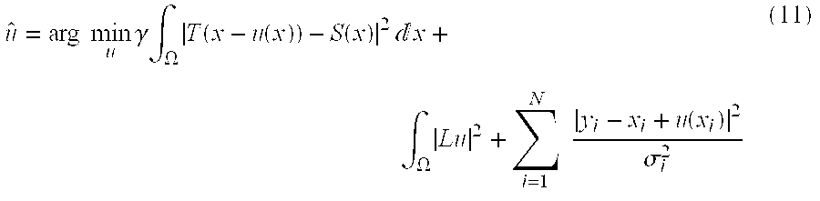
The foregoing steps of the image registration method provide a coarse matching of a template and a target image. Fine matching of the images requires using the full image data and the landmark information and involves selecting a distance measure by solving a synthesis equation that simultaneously maps selected image landmarks in the template and target images and matches all image points within a region of interest. An example of this synthesis equation is:
here the displacement field u is constrained to have the form
with the variables βi, A, and b, computed at step 350 in FIG. 3. The operator L in equation (11) may be the same operator used in equation (9), or alternatively, another operator may be used with a different set of boundary conditions. The basis functions φ are the eigen functions of operators such as the Laplacian Lu=∇2u, the bi-harmonic Lu=∇4u, linear elasticity Lu=α∇2u+(α+β)∇(∇.u), and powers of these operators LP for p ≧1.
One of ordinary skill in the art will recognize that there are many possible forms of the synthesis equation. For example, in the synthesis equation presented above, the distance measure in the first term measures the relative position of points in the target image with respect to points in the template image. Although this synthesis equation uses a quadratic distance measure, one of ordinary skill in the art will recognize that there are other suitable distance measures.
CPU 204 then computes a second or fusing transformation (Step 370) using the synthesis equation relating all points within a region of interest in the target image to all corresponding points in the template image. The synthesis equation is defined so that the resulting transform incorporates, or fuses, the mapping of manifold landmarks to corresponding target image points determined when calculating the first transform.
The computation using the synthesis equation is accomplished by solving a sequence of optimization problems from coarse to fine scale via estimation of the basis coefficients μ
k. This is analogous to multi-grid methods, but here the notion of refinement from coarse to fine is accomplished by increasing the number of basis components d. As the number of basis functions increases, smaller and smaller variabilities between the template and target are accommodated. The basis coefficients are determined by gradient descent, i.e.,
also Δ is a fixed step size and λk are the eigenvalues of the eigenvectors φk.
The computation of the fusion transformation (step 370) using the synthesis equation is presented in the flow chart of FIG. 8. Equation (12) is used to initialize the value of the displacement field u(x)=u(0)(x) (step 800). The basis coefficients μk=μk (0) are set equal to zero and the variables βi, A, and b are set equal to the solution of equation (11) (step 802). Equation (13) is then used to estimate the new values of the basis coefficients μk (n+1) given the current estimate of the displacement field u(n)(x) (step 804). Equation (15) is then used to compute the new estimate of the displacement field u(n)(x) given the current estimate of the basis coefficients μk (n) (step 806). The next part of the computation is to decide whether or not to increase the number d of basis functions φk used to represent the transformation (step 808). Increasing the number of basis functions allows more deformation. Normally, the algorithm is started with a small number of basis functions corresponding to low frequency eigen functions and then on defined iterations the number of frequencies is increased by one (step 810). This coarse-to-fine strategy matches larger structures before smaller structures. The preceding computations (steps 804-810) are repeated until the computation has converged or the maximum number of iterations is reached (step 812). The final displacement field is then used to transform the template image (step 814).
Once CPU 204 determines the transform from the synthesis equation fusing both landmark manifold information and image data, CPU 204 uses this transform to register the template image with the target image (step 380).
The spectrum of the second transformation, h, is highly concentrated around zero. This means that the spectrum mostly contains low frequency components. Using the sampling theorem, the transformation can be represented by a subsampled version provided that the sampling frequency is greater than the Nyquist frequency of the transformation. The computation may be accelerated by computing the transformation on a coarse grid and extending it to the full voxel lattice e.g., in the case of 3D images, by interpolation. The computational complexity of the algorithm is proportional to the dimension of the lattice on which the transformation is computed. Therefore, the computation acceleration equals the ratio of the full voxel lattice to the coarse computational lattice.
One of ordinary skill in the art will recognize that composing the landmark transformations followed by the elastic basis transformations, thereby applying the fusion methodology in sequence can provide an alternatively valid approach to hierarchial synthesis of landmark and image information in the segmentation.
Another way to increase the efficiency of the algorithm is to precompute the Green's functions and eigen functions of the operator L and store these precomputed values in a lookup table. These tables replace the computation of these functions at each iteration with a table lookup. This approach exploits the symmetry of Green's functions and eigen functions of the operator L so that very little computer memory is required. In the case of the Green's functions, the radial symmetry is exploited by precomputing the Green's function only along a radial direction.
The method described for fusing landmark information with the image data transformation can be extended from landmarks that are individual points (0-dimensional manifolds) to manifolds of dimensions 1, 2 and 3 corresponding to curves (1 -dimensional), surfaces (2-dimensional) and subvolumes (3-dimensional).
For example, FIG. 4 shows a template image 400 of a section of a brain with 1 - dimensional manifolds 402 and 404 corresponding to target image 406 1- dimensional manifolds 408 and 410 respectively. FIG. 5 shows a template image 500 of a section of a brain with 2-dimensional manifold 502 corresponding to target image 504 2-dimensional manifold 506. FIG. 6 shows a template image 600 of a section of a brain with 3-dimensional manifold 602 corresponding to target image 604 3-dimensional manifold 606.
As with the point landmarks, these higher dimensional manifolds condition the transformation, that is we assume that the vector field mapping the manifolds in the template to the data is given. Under this assumption the manually- assisted deformation (
step 350, FIG. 3) becomes the equality-constrained Bayesian optimization problem:
subject to
If M(i) is a smooth manifold for i=0, 1, 2, 3, the solution to this minimization is unique-satisfying L†Lû(x)=0, for all template points in the selected manifold. This implies that the solution can be written in the form of a Fredholm integral equation:
and G the Green's function of L.
When the manifold is a sub-volume, M(3),dS is the Lebesgue measure on R3. For 2-dimensional surfaces, dS is the surface measure on M(2), For 1-dimensional manifolds (curves), dS is the line measure on M(1) and for point landmarks, M(0), dS is the atomic measure. For point landmarks, the Fredholm integral equation degenerates into a summation given by equation (10).
When the manifold of interest is a smooth, 2-dimensional surface, the solution satisfies the classical Dirichlet boundary value problem:
L†Lû(x)=0,∀xεΩ\M (19)
The Dirichlet problem is solved using the method of successive over relaxation as follows. If uk(x) is the estimate of a deformation field at the kth iteration, the estimate at the (k+1)th iteration is given by the following update equation:
u k+1(x)=u k(x)+αL, † Lu(x), xεΩ\M
u k+1(x)=k(x), xεM, (20)
where α is the over relaxation factor.
It is also possible to- compute the transform (step 370) with rapid convergence by solving a series of linear minimization problems where the solution to the series of linear problems converges to the solution of the nonlinear problem. This avoids needing to solve the nonlinear minimization problem directly. Using a conjugate gradient method, the computation converges faster than a direct solution of the synthesis equation because the basis coefficients μk are updated with optimal step sizes.
Using the conjugate gradient, the displacement field is assumed to have the form
where
Begin by assuming that ƒ(x) is fixed. This is generalized below. The eigen functions in the expansion are all real and follow the assumption that {φi (x)} are R3 valued.
The minimization problem is solved by computing
μj new=μj old+Δj=0 . . . d (23)
to update the basis coefficients in equation (21) where μ
j=0,j=0 . . . d initially, Δ
j is computed using the equation
where h
i (x)=∇T|
x−u(x)·φ
i(x), and where θ
ij (x)=φ
j (x)·φ
j (x). The notation f·g is the inner-product, i.e.,
Similarly, since u(x) is written in the series expansion given in equations (21) and (22), the identical formulation for updating βi arises. Accordingly, the fusion achieved by the present invention results. Computation of equation (23) repeats until all Δj fall below a predetermined threshold solving for each Δj in sequence of increasing j, and Δ4, is computed using the values of Δk for 0≦k<j.
A further improvement over prior art image registration methods is achieved by computing the required transforms using fast Fourier transforms (FFT). Implementing an FFT based computation for image registration using a synthesis equation, as required at step 370 of FIG. 3, provides computational efficiency. However, to exploit the known computational efficiencies of FFT transforms, the solution of the synthesis equation must be recast to transform the inner products required by iterative algorithms into shift invariant convolutions.
To make the inner-products required by the iterative algorithms into shift invariant convolution, differential and difference operators are defined on a periodic version of the unit cube and the discrete lattice cube. Thus, the operators are made cyclo-stationary, implying their eigen functions are always of the form of complex exponentials on these cubes having the value:
r=1, 2, 3 with x=(x1, x2, x3)ε[0, 1]3, ωki=2πki, i=1, 2, 3, and the Fourier basis for periodic functions on [0, 1]3 takes the form
j<ω k ,x>, ωkx>=ωk 1 x1+ωk 2 x2+ωk 3 x3 k=(ωk 1 ,ωk 2 ,ωk 3
On the discrete N
3=periodic lattice,
For real expansions, the eigen vectors becomes φ
k(x)=Ψ
k(x)+Ψ
k*(x) and the real expansion in equation (21) becomes:
where * means complex conjugate, and
This reformulation supports an efficient implementation of the image registration process using the FFT. Specifically, if step 370 of FIG. 3, computing the registration transform fusing landmark and image data, is implemented using the conjugate gradient method, the computation will involve a series of inner products. Using the FFT exploits the structure of the eigen functions and the computational efficiency of the FFT to compute these inner-products.
For example, one form of a synthesis equation for executing
Step 370 of FIG. 3 will include the following three terms:
Each of theses terms must be recast in a suitable form for FFT computation. One example of a proper reformulation for each of these terms is:
Term 1:
where
This equation is computed for all k by a Fourier transformation of the function.
and hence can be computed efficiently using a 3-D FFT.
Term 2:
The integral in the above summation for all k can be computed by Fourier transforming the elements of the 3×3 matrix:
∇T(∇T)t (30)
evaluated at ωk+ωj. Because this matrix has diagonal symmetry, the nine FFTs in this reformulation of term 2 can be computed efficiently using six three dimensional FFTs evaluated at ωk+ωj.
Term 3:
Using the exact form for the eigen functions we can rewrite the above equation as
This summation is precisely the inverse Fourier transforms of the functions
and hence can be computed efficiently by using a 3-D FFT.
One of ordinary skill in the art will recognize that restructuring the computation of registration transforms using FFTs will improve the performance of any image registration method having terms similar to those resulting from a synthesis equation fusing landmark and image data. Improvement results from the fact that many computer platforms compute FFTs efficiently; accordingly, reformulating the registration process as an FFT computation, makes the required computations feasible.
A distance function used to measure the disparity between images is the Gaussian square error distance ∫ |T(x−u(x))−S(x)|2dx. There are many other forms of an appropriate distance measure. More generally, distance functions, such as the correlation distance, or the Kullback Liebler distance, can be written in the form ∫ D(T(x−u(x)), S(x))dx.
An efficient convolution implementation can be derived using the FFT for arbitrary distance functions. Computing the fusing transform using the image data follows the equation:
where D(.,.) is a distance function relating points in the template and target images. The displacement field is assumed to have the form:
is fixed. The basis coefficients {μ
k} are determined by gradient descent, i.e.,
where the gradient is computed using the chain rule and is given by the equation
where D′ (.,.)is the derivative with respect to the first argument. The most computationally intensive aspect of the algorithm is the computation of the term
Using the structure of the eigen functions and the computational efficiency of the FFT to compute these inner-products, the above term can be written as
where
This equation is computed for all k by a Fourier transformation of the function
and hence can be computed efficiently using a 3-D FFT.
The following example illustrates the computational efficiencies achieved using FFTs for image registration instead of direct computation of inner-products. Assuming that a target image is discretized on a lattice having N3 points, each of the inner-products in the algorithm, if computed directly, would have a computational complexity of the order (N3)2. Because the inner-products are computationally intensive, the overall complexity of image registration is also (N3)2. In contrast, each of the FFTs proposed has a computational complexity on the order of N3log2 N3. The speed up is given by the ratio N6/(N3log2 N3)=N3/(3 log2 N). Thus the speed up is 64 times for a 16×16×16 volume and greater than 3.2×10⁴ speed up for a 256×256×256 volume.
A further factor of two savings in computation time can be gained by exploiting the fact that all of the FFTs are real. Hence all of the FFTs can be computed with corresponding complex FFTs of half the number of points. For a development of the mathematics of FFTs see, A. V. Oppenheim and R. W. Schafer, Digital Signal Processing, Prentice-Hall, N.J., 1975 (hereinafter referred to as Oppenheim).
Alternative embodiments of the registration method described can be achieved by changing the boundary conditions of the operator. In the disclosed embodiment, the minimization problem is formulated with cyclic boundary conditions. One of ordinary skill in the art will recognize that alternative boundary conditions, such as the Dirichlet, Neumann, or mixed Dirichlet and Neumann boundary conditions are also suitable. The following equation is used in an embodiment of the present invention using one set of mixed Dirichlet and Neumann boundary conditions:
where the notation (x|x
i=k) means x is in the template image such that x
i=k. In this case, the eigen functions would be of the form:
Modifying boundary conditions requires modifying the butterflies of the FFT from complex exponentials to appropriate sines and cosines.
In FIG. 7, four images, template image 700, image 704, image 706, and target image 708, illustrate the sequence of registering a template image and a target image. Template image 700 has 0-dimensional landmark manifolds 702. Applying the landmark manifold transform computed at step 350 in FIG. 3 to image 700 produces image 704. Applying a second transform computed using the synthesis equation combining landmark manifolds and image data to image 700 produces image 706. Image 706 is the final result of registering template image 700 with target image 708. Landmark manifold 710 in image 708 corresponds to landmark manifold 702 in template image 700.
Turning now to techniques to register images which may possess large deformation characteristics using diffeomorphisms, large deformation transform functions and transformations capable of matching images where the changes from one image to the other are greater than small, linear, or affine. Use of large deformation transforms provide for the automatic calculation of tangents, curvature, surface areas, and geometric properties of the imagery.
2. Methods for Large Deformation Landmark Based and Image Based Transformations
An embodiment consistent with the present invention maps sets of landmarks in imagery {xi, i=1,2, . . . , N} ⊂Ω into target landmarks {yi, i=1, . . . , N}, and or imagery I0 into target I1, both with and without landmarks. For example when there is a well-defined distance function D(u(T)) expressing the distance between the landmarks and or imagery. The large deformation maps h: Ω→Ω are constructed by introducing the time variable,
h: (x, t)=(x1,x2,x3, t)εΩ×[0,T]→h(x,t)=(x 1 −u 1(x,t),x 2 −u 2(x,t),x 3 −u 3(x,t))εΩ.
The large deformation maps are constrained to be the solution h(x, T)=x−u(x, T) where u(x, T) is generated as the solution of the ordinary differential equation
assuming that the {φk} forms a complete orthonormal base.
Then a diffeomorphism for the landmark and image matching problems is given by the mapping of the imagery given by ĥ(x, T)=x−û(x, T) satisfying the Ordinary Differential Equation (O.D.E.)
L is preferably a linear differential operator with the k forming a complete orthonormal base as the eigen functions Lφk=λkφk.
2.1 Large Deformation Landmark Matching
In order to register images with large deformation using a landmark matching technique, N landmarks are identified in the two anatomies target {x
i, y
i, i=1, 2, . . . , N}. The landmarks are identified with varying degrees of accuracy {Σ
i, i=1, . . . , N), the Σ
i, 3×3 covariance matrices. The distance between the target and template imagery landmarks preferably used is defined to be
A preferable diffeomorphism is the minimizer of Eqns. 40, 41 with D(u(T)) the landmark distance:
A method for registering images consistent with the present invention preferably includes the following steps:
STEP 0: Define a set of landmarks in the template which can be easily identified in the target {xi:xiεΩ, i=1, 2, . . . , N} with varying degrees of accuracy in the target as {yi, i=1, . . . , N} with associated error covariance {Σi, i=1, . . . , N}, and initialize for n=0, v.=0.
STEP 1: Calculate velocity and deformation fields:
STEP 2: Solve via a sequence of optimization problems from coarse to fine scale via estimation of the basis coefficients {v
k}, analogous to multi-grid methods with the notion of refinement from coarse to fine accomplished by increasing the number of basis components. For each v
k,
STEP 3: Set n←n+1, and return to Step 1.
2.2 Large Deformation Image Matching
Turning now to the technique where a target and template image with large deformation are registered using the image matching technique. The distance between the target and template image is chosen in accordance with Eqn. 47. A diffeomorphic map is computed using an image transformation operator and image transformation boundary values relating the template image to the target image. Subsequently the template image is registered with the target image using the diffromorphic map.
Given two images I0, I1, choose the distance
D 2(u(T))≐γ∫[0,1] 3 |I 0(x−u(x,T))−I 1(x)|2 dx. (47)
The large deformation image distance driven map is constrained to be the solution ĥ(x,T)=x−û(x,T) where
A method for registering images consistent with the present invention preferably includes the following steps:
STEP 0: Measure two images I0, I1 defined on the unit cube Ω≐[0,1]3⊂R3, initialize parameters for n=0, vk (n)=0, k=0, 1, . . . , and define distance measure D(u(T)) Eqn. 47.
STEP 1: Calculate velocity and deformation fields from v
(n):
STEP 2: Solve optimization via sequence of optimization problems from coarse to fine scale via re-estimation of the basis coefficients {v
k}, analogous to multi-grid methods with the notion of refinement from coarse to fine accomplished by increasing the number of basis components. For each v
k,
STEP 3: Set n←n+1, and return to Step 1.
The velocity field can be constructed with various boundary conditions, for example v(x,t)=0, x ε∂Ω and t ε[0, T], u(x, 0)=v(x, 0)=0. The differential operator L can be chosen to be any in a class of linear differential operators; we have used operators of the form (−aΔ−b∇∇·+cl)
P, p≧1. The operators are 3×3 matrices
2.3 Small deformation solution
The large deformation computer algorithms can be related to the small deformation approach described in the '628 application, by choosing v=u, so that T=δ small, then approximate I−∇u(·,σ)≈I for σε[0, δ), then û(x, δ)=v(x)δ and defining u(x)≐u(x, δ), so that Eqn. 55 reduces to the small deformation problems described in the '628 application:
3. Composing Large Deformation Transformations Unifying Landmark and Image Matching
The approach for generating a hierarchical transformation combining information is to compose the large deformation transformations which are diffeomorphisms and can therefore be composed, h=hn∘ . . . h2 ∘h1. Various combinations of transformations may be chosen, including the affine motions, rigid motions generated from subgroups of the generalized linear group, large deformation landmark transformations which are diffeomorphisms, or the high dimensional large deformation image matching transformation. During these, the dimension of the transformations of the vector fields are being increased. Since these are all diffeomorphisms, they can be composed.
4. Fast Method for Landmark Deformations Given Small Numbers of Landmarks For small numbers of landmarks, we re-parameterize the problem using the Lagrangian frame, discretizing the optimization over space time Ω×T, into N functions of time T. This reduces the complexity by order of magnitude given by the imaging lattice [Ω].
For this, define the Lagrangian positions of the N-landmarks x
i, i=1, . . . , N as they flow through time φ
i(·), i=1, . . . , N, with the associated 3N-vector
The particle flows Φ(t) are defined by the velocities v(·) according to the fundamental O.D.E.
It is helpful to define the 3N×3N covariance matrix K(Φ(t)):
The inverse K(Φ(t))−1 is an N×N matrix with 3×3 block entries (K(Φ(t))−1)ij, i, j=1, . . . , N.
For the landmark matching problem, we are given N landmarks identified in the two anatomies target {xi, yi, i=1, 2, . . . , N}, identified with varying degrees of accuracy {Σi, i=1, . . . N}, the Σi, 3×3 covariance matrices.
The squared error distance between the target and template imagery defined in the Lagrangian trajectories of the landmarks becomes
Then a preferable diffeomorphism is the minimizer of Eqns. 40, 41 with D
1(Φ(T)) the landmark distance:
A fast method for small numbers of Landmark matching points exploits the fact that when there are far fewer landmarks N than points in the image x ε Ω, there is the following equivalent optimization problem in the N-Lagrangian velocity fields φ(x
i, ·), I=1, . . . , N which is more computationally efficient than the optimization of the Eulerian velocity v(x
i,·),x ε Ω, (|Ω|>>N). Then, the equivalent optimization problem becomes
This reduces to a finite dimensional problem by defining the flows on the finite grid of times, assuming step-size δ with Lagrangian velocities piecewise constant within the quantized time intervals:
Then the finite dimensional minimization problem becomes
subject to: φ(xi, 0)=xi, i=1, . . . , N
The Method:
In order to properly register the template image with the target image when a small number of landmarks have been identified, the method of the present embodiment utilizes the Largrangian positions. The method for registering images consistent with the present invention includes the following steps:
STEP 0: Define a set of landmarks in the template which can be easily identified in the target {xi:xi εΩ, i=1,2, . . . , N), with varying degrees of accuracy in the target as {yi, i=1, . . . , N} with associated error covariance {Σi, i=1, . . . , N},and initialize for n=0, φ(n)(xi, ·)=xi.
STEP 1: Calculate velocity and deformation fields:
STEP 2: Solve via estimation of the Lagrangian positions φ(k),k=1, . . . , K.
For each φ(x
i, k),
STEP 3: Set n←n+1, and return to Step 1.
STEP 4: After stopping, then compute the optimal velocity field using equation 62 and transform using equation 64.
5. Fast Greedy Implementation of Large Deformation Image Matching
For the image matching, discretize space-time Ω×T into a sequence of indexed in time optimizations, solving for the locally optimal at each time transformation and then forward integrate the solution. This reduces the dimension of the optimization and allows for the use of Fourier transforms.
The transformation h(·, t):Ω→Ω where h(x, t)=x−u(x, t), and the transformation and velocity fields are related via the O.D.E.
Preferably the deformation fields are generated from the velocity fields assumed to be piecewise constant over quantized time increments,
the quantized time increment. Then the sequence of deformations u(x,t
i),i=1, . . . I is given by
For δ small, approximate ∇u(x,σ)≈∇u(x,t
i),σε[t
i,t
i+1], then the global optimization is solved via a sequence of locally optimal solutions according to for t
i, I=1, . . . , I,
The sequence of locally optimal velocity fields {circumflex over (v)}(x,ti),i=1, . . . I satisfy the O.D.E.
L † L{circumflex over (v)}(x,t i+1))where û(x,t i+1)=û(x,t i)+δ(I−∇û(x,t i)){circumflex over (v)}(x,t i). (70)
Examples of boundary conditions include v(x,t)=0, x ε ∂Ω and t ε[0,T] and L the linear differential operator L=−a ∇2−b∇·∇+cI. The body force b(x−u(x,t)) is given by the variation of the distance D(u) with respect to the field at time t. The PDE is solved numerically (G. E. Christensen, R. D. Rabbitt, and M. I. Miller, “Deformable templates using large deformation kinematics,” IEEE Transactions on Image Processing, 5(10):1435-1447, Oct. 1996 for details (hereinafter referred to as Christensen).
To solve for fields u(·, t
i) at each t
i, expand the velocity fields Σ
kV
k(t
i)φ
k(·). v(·,t
i)=Σ
kVk(t
i)φk(·). To make the inner-products required by the iterative algorithms into shift invariant convolution, force the differential and difference operators L to be defined on a periodic version of the unit cube Ω≐[0,1 ]
3 and the discrete lattice cube {0,1, . . . , N−1}
3. f·g denotes the inner-product f·g=Σ
3 i=1 f
ig
i for f,g ε R
3. The operators are cyclo-stationary in space, implying their eignen functions are of the form of complex exponentials on these cubes:
(ω
k1,ω
k2,ω
k3),ω
k 1 =2πk
ii=1,2,3, and the Fourier basis for periodic functions on [0,1]
3 takes the form e
j<ω k ,x>, <ω
k,x>=ω
k1x
1+ω
k2x
2+ω
k3x
3. On the discrete N
3=periodic lattice,
This supports an efficient implementation of the above algorithm exploiting the Fast Fourier Transform (FFT).
Suppressing the d subscript on v
k,d and the summation from d=1 to 3 for the rest of this section simplifies notation. The complex coefficients v
k(t
i)=a
k(t
i)+b
k(t
i) have complex-conjugate symmetry because they are computed by taking the FFT of a real valued function as seen later in this section. In addition, the eigen functions have complex-conjugate symmetry due to the 2π periodicity of the complex exponentials. Using these two facts, it can be shown that the vector field
is R
3valued even though both v
k(t
i) and φ
k(x) are complex valued. The minimization problem is solved by computing for each v
k=a
k+b
k,
and g
kε{a
k, b
k}. Combining Eqs. 70 and 71 and taking derivatives gives
Consider the computation of the following terms of the algorithm from equations 73,
Computation of Term 1: The first term given by
can be written as
This equation can be computed efficiently using three 3D FFTs of the form
and s=1,2,3. These FFTs are used to evaluate Eq. 72 by noticing:
Computation of Term 2:
The second term given by
can be computed efficiently using three 3D FFTs. Specifically the 3D FFTs are
Using the FFT to compute the terms in the method provides a substantial decrease in computation time over brute force computation. For example, suppose that one wanted to process 2563 voxel data volumes. The number of iterations is the same in both the FFT and brute force computation methods and therefore does not contribute to our present calculation. For each 3D summation in the method, the brute force computation requires on the order N6 computations while the FFT requires on the order 3N3log2(N) computations. For N3=2563 voxel data volumes this provides approximately a 7×10⁵ speed up for the FFT algorithm compared to brute force calculation.
6. Rapid Convergence Algorithm for Large Deformation Volume Transformation
Faster converging algorithms than gradient descent exist such as the conjugate gradient method for which the basis coefficients vk are updated with optimal step sizes.
The identical approach using FFTs follows as in the '628 application. Identical speed-ups can be accomplished; see the '628 application.
6.1 An extension to general distance functions
Thus far only the Gaussian distance function has been described measuring the disparity between imagery has been described |I0(x−u(x))−1(x)|2d . More general distance functions can be written as ∫D(I0(x−u(x))),I1(x))dx. A wide variety of distance functions are useful for the present invention such as the correlation distance, or the Kullback Liebler distance can be written in this form.
6.2 Computational Complexity
The computational complexity of the methods herein described is reduced compared to direct computation of the inner-products. Assuming that the image is discretized on a lattice of size N3 each of the inner-products in the algorithm, if computed directly, would have a computational complexity of O((N3)2). As the inner-products are most computationally intensive, the overall complexity of the method is O((N3)2). Now in contrast, each of the FFTs proposed have a computational complexity of O(N3log2N3), and hence the total complexity of the proposed algorithm is O(N3log2N3). The speed up is given by the ratio N6/(N3log2 N3)=N3/(3 log2N). Thus the speed up is 64 times for 16×16×16 volume and greater than 3.2×10⁴ speed up for a 256×256×256 volume.
A further factor of two savings in computation time can be gained by exploiting the fact that all of the FFTs are real. Hence all of the FFTs can be computed with corresponding complex FFTs of half the number of points (see Oppenheim).
6.3 Boundary Conditions of the Operator
Additional methods similar to the one just described can be synthesized by changing the boundary conditions of the operator. In the previous section, the minimization problem was formulated with cyclic boundary conditions. Alternatively, we could use the mixed Dirichlet and Neumann boundary conditions corresponding to ∂u
i/∂x
i|(x|x
i=k)=u
i(x|x
j=k)=0 for i,j=1,2,3; i≠j; k=0,1 where the notation (x|x
i=k) means x ε Ω such that x
i=k. In this case the eigen functions would be of the form
The implementation presented in Section 5 is modified for different boundary conditions by modifying the butterflys of the FFT from complex exponentials to appropriate sines and cosines.
7. Apparatus for Image Registration
FIG. 2 shows an apparatus to carry out an embodiment of this invention. A medial imaging scanner 214 obtains image 100 and 120 and stores them in computer memory 206 which is connected to computer control processing unit (CPU) 204. One of the ordinary skill in the art will recognize that a parallel computer platform having multiple CPUs is also a suitable hardware platform for the present invention, including, but not limited to, massively parallel machines and workstations with multiple processors. Computer memory 206 can be directly connected to CPU 204, or this memory can be remotely connected through a communications network.
The method described herein use information either provided by an operator, stored as defaults, or determined automatically about the various substructures of the template and the target, and varying degrees of knowledge about these substructures derived from anatomical imagery, acquired from modalities like CT, MRI, functional MRI, PET, ultrasound, SPECT, MEG, EEG, or cryosection. For example, an operator can guide cursor 210 using pointing device 208 to select in image 100.
The foregoing description of the preferred embodiments of the present invention has been provided for the purpose of illustration and description. It is not intended to be exhaustive or to limit the invention to the precise forms disclosed. Obviously many modifications, variations and simple derivations will be apparent to practitioners skilled in the art. The embodiments were chosen and described in order to best explain the principles of the invention and its practical application, thereby enabling others skilled in the art to understand the invention for various embodiments and with various modifications are suited to the particular use contemplated. It is intended that the scope of the invention be defined by the following claims and their equivalents.