WO2018212115A1 - 組織の粘弾性を断層可視化する装置および方法 - Google Patents
組織の粘弾性を断層可視化する装置および方法 Download PDFInfo
- Publication number
- WO2018212115A1 WO2018212115A1 PCT/JP2018/018455 JP2018018455W WO2018212115A1 WO 2018212115 A1 WO2018212115 A1 WO 2018212115A1 JP 2018018455 W JP2018018455 W JP 2018018455W WO 2018212115 A1 WO2018212115 A1 WO 2018212115A1
- Authority
- WO
- WIPO (PCT)
- Prior art keywords
- tissue
- viscoelasticity
- deformation
- optical
- light
- Prior art date
Links
Images
Classifications
-
- A—HUMAN NECESSITIES
- A61—MEDICAL OR VETERINARY SCIENCE; HYGIENE
- A61B—DIAGNOSIS; SURGERY; IDENTIFICATION
- A61B5/00—Measuring for diagnostic purposes; Identification of persons
- A61B5/0059—Measuring for diagnostic purposes; Identification of persons using light, e.g. diagnosis by transillumination, diascopy, fluorescence
- A61B5/0062—Arrangements for scanning
- A61B5/0066—Optical coherence imaging
-
- G—PHYSICS
- G01—MEASURING; TESTING
- G01B—MEASURING LENGTH, THICKNESS OR SIMILAR LINEAR DIMENSIONS; MEASURING ANGLES; MEASURING AREAS; MEASURING IRREGULARITIES OF SURFACES OR CONTOURS
- G01B9/00—Measuring instruments characterised by the use of optical techniques
- G01B9/02—Interferometers
- G01B9/0209—Low-coherence interferometers
- G01B9/02091—Tomographic interferometers, e.g. based on optical coherence
-
- A—HUMAN NECESSITIES
- A61—MEDICAL OR VETERINARY SCIENCE; HYGIENE
- A61B—DIAGNOSIS; SURGERY; IDENTIFICATION
- A61B1/00—Instruments for performing medical examinations of the interior of cavities or tubes of the body by visual or photographical inspection, e.g. endoscopes; Illuminating arrangements therefor
-
- A—HUMAN NECESSITIES
- A61—MEDICAL OR VETERINARY SCIENCE; HYGIENE
- A61B—DIAGNOSIS; SURGERY; IDENTIFICATION
- A61B5/00—Measuring for diagnostic purposes; Identification of persons
- A61B5/0033—Features or image-related aspects of imaging apparatus classified in A61B5/00, e.g. for MRI, optical tomography or impedance tomography apparatus; arrangements of imaging apparatus in a room
- A61B5/004—Features or image-related aspects of imaging apparatus classified in A61B5/00, e.g. for MRI, optical tomography or impedance tomography apparatus; arrangements of imaging apparatus in a room adapted for image acquisition of a particular organ or body part
-
- A—HUMAN NECESSITIES
- A61—MEDICAL OR VETERINARY SCIENCE; HYGIENE
- A61B—DIAGNOSIS; SURGERY; IDENTIFICATION
- A61B5/00—Measuring for diagnostic purposes; Identification of persons
- A61B5/44—Detecting, measuring or recording for evaluating the integumentary system, e.g. skin, hair or nails
- A61B5/441—Skin evaluation, e.g. for skin disorder diagnosis
- A61B5/442—Evaluating skin mechanical properties, e.g. elasticity, hardness, texture, wrinkle assessment
-
- A—HUMAN NECESSITIES
- A61—MEDICAL OR VETERINARY SCIENCE; HYGIENE
- A61B—DIAGNOSIS; SURGERY; IDENTIFICATION
- A61B8/00—Diagnosis using ultrasonic, sonic or infrasonic waves
- A61B8/08—Detecting organic movements or changes, e.g. tumours, cysts, swellings
-
- G—PHYSICS
- G01—MEASURING; TESTING
- G01B—MEASURING LENGTH, THICKNESS OR SIMILAR LINEAR DIMENSIONS; MEASURING ANGLES; MEASURING AREAS; MEASURING IRREGULARITIES OF SURFACES OR CONTOURS
- G01B11/00—Measuring arrangements characterised by the use of optical techniques
- G01B11/16—Measuring arrangements characterised by the use of optical techniques for measuring the deformation in a solid, e.g. optical strain gauge
- G01B11/161—Measuring arrangements characterised by the use of optical techniques for measuring the deformation in a solid, e.g. optical strain gauge by interferometric means
-
- G—PHYSICS
- G01—MEASURING; TESTING
- G01N—INVESTIGATING OR ANALYSING MATERIALS BY DETERMINING THEIR CHEMICAL OR PHYSICAL PROPERTIES
- G01N21/00—Investigating or analysing materials by the use of optical means, i.e. using sub-millimetre waves, infrared, visible or ultraviolet light
- G01N21/17—Systems in which incident light is modified in accordance with the properties of the material investigated
-
- G—PHYSICS
- G01—MEASURING; TESTING
- G01N—INVESTIGATING OR ANALYSING MATERIALS BY DETERMINING THEIR CHEMICAL OR PHYSICAL PROPERTIES
- G01N29/00—Investigating or analysing materials by the use of ultrasonic, sonic or infrasonic waves; Visualisation of the interior of objects by transmitting ultrasonic or sonic waves through the object
- G01N29/04—Analysing solids
- G01N29/06—Visualisation of the interior, e.g. acoustic microscopy
- G01N29/0654—Imaging
- G01N29/0672—Imaging by acoustic tomography
-
- G—PHYSICS
- G01—MEASURING; TESTING
- G01N—INVESTIGATING OR ANALYSING MATERIALS BY DETERMINING THEIR CHEMICAL OR PHYSICAL PROPERTIES
- G01N29/00—Investigating or analysing materials by the use of ultrasonic, sonic or infrasonic waves; Visualisation of the interior of objects by transmitting ultrasonic or sonic waves through the object
- G01N29/22—Details, e.g. general constructional or apparatus details
- G01N29/24—Probes
- G01N29/2418—Probes using optoacoustic interaction with the material, e.g. laser radiation, photoacoustics
-
- G—PHYSICS
- G01—MEASURING; TESTING
- G01N—INVESTIGATING OR ANALYSING MATERIALS BY DETERMINING THEIR CHEMICAL OR PHYSICAL PROPERTIES
- G01N2291/00—Indexing codes associated with group G01N29/00
- G01N2291/02—Indexing codes associated with the analysed material
- G01N2291/028—Material parameters
- G01N2291/02818—Density, viscosity
-
- G—PHYSICS
- G01—MEASURING; TESTING
- G01N—INVESTIGATING OR ANALYSING MATERIALS BY DETERMINING THEIR CHEMICAL OR PHYSICAL PROPERTIES
- G01N2291/00—Indexing codes associated with group G01N29/00
- G01N2291/02—Indexing codes associated with the analysed material
- G01N2291/028—Material parameters
- G01N2291/02827—Elastic parameters, strength or force
Definitions
- the present invention relates to an apparatus and method capable of displaying a tomographic display of viscoelasticity of a tissue to be measured on a microscale.
- OCT optical coherence tomography
- a tomographic method using low-coherence optical interference can visualize the morphological distribution of a living tissue with high spatial resolution on a micro scale.
- the acquisition rate of two-dimensional OCT is equal to or higher than the video rate, and has a high temporal resolution.
- Patent Document 1 a method for visualizing the mechanical properties of a living tissue using tomography using OCT.
- OCT optical coherence tomography
- Patent Document 1 When performing such mechanical characteristic evaluation, an algorithm for deforming a living tissue is incorporated in OCT measurement. For this reason, the technique of Patent Document 1 employs a method in which a piezoelectric element is brought into contact with the surface of a measurement object and loaded.
- a measurement object that requires strict quality assurance such as a regenerative tissue
- such contact of the piezoelectric element may cause tissue contamination and hinder the practical use of the system. Based on such knowledge, the inventor has realized that the OCT system needs to be improved.
- the present invention has been made in view of such problems, and one of its purposes is to provide a technique that enables mechanical property evaluation by OCT measurement even for a measurement object that requires strict quality assurance. There is.
- a certain aspect of the present invention relates to a viscoelasticity visualization apparatus that includes an optical system using OCT and visualizes the viscoelasticity of a tissue in a measurement target by a tomography.
- This device controls the drive of the optical mechanism for guiding the light from the light source to the tissue for scanning, the load device for applying deformation energy to the tissue, and the drive of the load device and the optical mechanism.
- a control calculation unit that calculates a tomographic distribution of the viscoelasticity of the tissue by processing an optical interference signal by the optical system based on the above, and a display device that displays the viscoelasticity of the tissue in a manner of visualizing the tomogram.
- the load device is a non-contact load device that loads an excitation force by an acoustic radiation pressure on a tissue by outputting an ultrasonic wave toward a focal point set inside the measurement target.
- Another aspect of the present invention relates to a viscoelasticity visualization method for visualizing a viscoelasticity of a tissue to be measured by a tomography.
- This method obtains an optical interference signal based on backscattered light from a tissue that is deformed by a load by using a loading process in which a load is applied to the tissue with ultrasonic acoustic radiation pressure and OCT.
- One embodiment of the present invention is a viscoelasticity visualization apparatus using OCT.
- This device includes a light source, an optical mechanism, a load device, a control calculation unit, and a display device, and visualizes the viscoelasticity of the tissue in the measurement target by tomography.
- the “measurement target” may be a living tissue such as skin or cartilage, or may be a regenerated tissue (tissue composed of cultured cells) such as regenerated skin or regenerated cartilage.
- the load device outputs an ultrasonic wave toward a focal point set inside the measurement target, and loads an acoustic radiation pressure on the tissue.
- the focal point is a point where the excitation force due to the acoustic radiation pressure is concentrated inside the measurement object, and is set by the control calculation unit.
- the load by acoustic radiation pressure and the detection by OCT are performed.
- the load due to the acoustic radiation pressure may be a dynamic load (excitation force). It is possible to induce a tissue deformation by applying a load in a non-contact manner to a desired tomographic position to be measured by acoustic radiation pressure.
- OCT enables tomographic measurement in a non-contact / non-invasive manner. That is, according to this aspect, both the load device and the optical mechanism can be made non-contact with respect to the measurement target. For this reason, even if the measurement target requires strict quality assurance, the contamination can be prevented and the mechanical properties (viscoelasticity) can be evaluated.
- the axis of light irradiated toward the measurement target may be set so as to pass through the focal point of the acoustic radiation pressure on the measurement target. Thereby, the deformation of the tissue at the focal position can be detected directly and in real time.
- the optical axis may be set at a predetermined distance from the focal point, and a viscoelasticity evaluation standard corresponding to the distance may be set.
- the control calculation unit calculates a predetermined mechanical feature amount caused by the tissue deformation or a change in the mechanical feature amount due to the tissue deformation in association with the tomographic position of the measurement target, and based on the calculation result, the viscoelasticity of the tissue
- the fault distribution may be calculated.
- the “mechanical feature amount” here may be obtained based on the deformation amount or deformation vector of the tissue.
- a strain tensor obtained by spatially differentiating the deformation vector may be used. It may be the amplitude or phase of distortion. Alternatively, it may be a deformation rate vector obtained by temporally differentiating the deformation vector, or a strain rate tensor obtained by further spatially differentiating the deformation rate vector. Their amplitude or phase may be used.
- the viscoelasticity may be calculated based on the amplitude of the excitation force due to the acoustic radiation pressure, the amplitude of the strain detected by the OCT, and the phase difference between them. Since the excitation force due to the acoustic radiation pressure is generated by driving the load device, it can be used that the amplitude and phase of the excitation force are known.
- the magnitude (amplitude value) of the deformation rate (strain rate) with respect to the load variation and the follow-up property (responsiveness) of the deformation rate (strain rate) with respect to the fluctuation of the excitation force Tend to change.
- the amplitude value of the deformation speed (strain speed) increases and the time delay (phase delay) tends to decrease. Viscoelasticity can also be evaluated based on such a tendency.
- a shear wave generated by applying ultrasonic waves to the measurement target may be detected as a fault, and the viscoelasticity of the tissue may be calculated from the propagation speed.
- Non-contact elastography using acoustic radiation pressure is used to detect tissue viscoelasticity by OCT.
- the optical mechanism may emit light from the front side of the measurement target, and the load device may output ultrasonic waves from the back side of the measurement target. Thereby, it becomes easy to prevent physical interference between the optical mechanism and the load device, and the design of the device becomes easy.
- a support base that supports a container that stores the regenerated tissue may be provided.
- this container one having translucency and sound wave permeability may be adopted, and a hole for exposing the back side of the container may be provided in the support base.
- the container is preferably sealable for quality assurance of the regenerated tissue. You may arrange
- This device may include a first optical mechanism, a second optical mechanism, and a light detection device.
- the first optical mechanism is provided in an object arm that passes through the measurement target, and guides light from the light source to the measurement target to be scanned.
- the second optical mechanism is provided in a reference arm that does not pass through the measurement target, and guides and reflects light from the light source to the reference mirror.
- the light detection device detects interference light in which the object light reflected by the measurement target and the reference light reflected by the reference mirror are superimposed.
- the control calculation unit performs frequency analysis on the optical interference signal input from the light detection device, and calculates the deformation rate of the tissue using the Doppler frequency.
- the viscoelasticity may be calculated based on strain information obtained based on the deformation speed and acoustic radiation pressure information obtained from the load device.
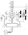
- FIG. 1 is a diagram schematically illustrating a configuration of a viscoelasticity visualization apparatus according to an embodiment.
- the apparatus of the present embodiment visualizes the viscoelasticity of the regenerated tissue by measuring the tomography on a micro scale. For this tomographic measurement, load by acoustic radiation pressure and detection by OCT are used.
- the OCT apparatus 1 includes a light source 2, an object arm 4, a reference arm 6, optical mechanisms 8 and 10, a light detection device 12, a load device 13, a control calculation unit 14, and a display device 16.
- Each optical element is connected to each other by an optical fiber.
- an optical system based on a Mach-Zehnder interferometer is shown, but a Michelson interferometer or other optical system can also be adopted.
- TD-OCT Time Domain OCT
- SS-OCT Sewept Source OCT
- SD-OCT Spectrum Domain OCT
- the light emitted from the light source 2 is divided by a coupler 18 (beam splitter), one of which is guided to the object arm 4 to become object light, and the other is guided to the reference arm 6 to become reference light.
- the object light of the object arm 4 is guided to the optical mechanism 8 via the circulator 20 and is irradiated onto a measurement target (hereinafter referred to as “target S”).
- the target S is a regenerated tissue (cultured tissue) in this embodiment. This object light is reflected as backscattered light on the surface and cross section of the target S, returns to the circulator 20, and is guided to the coupler 22.
- the reference light of the reference arm 6 is guided to the optical mechanism 10 via the circulator 24.
- This reference light is reflected by the reference mirror 26 of the optical mechanism 10, returns to the circulator 24, and is guided to the coupler 22. That is, the object light and the reference light are combined (superimposed) by the coupler 22, and the interference light is detected by the light detection device 12.
- the light detection device 12 detects this as an optical interference signal (a signal indicating the intensity of interference light).
- This optical interference signal is input to the control calculation unit 14 via the A / D converter 28.
- the control calculation unit 14 performs control processing for the entire optical system, control of the load device (ultrasonic vibration device), and image output by OCT.
- the command signal of the control calculation unit 14 is input to the light source 2, the optical mechanisms 8 and 10, the load device 13, and the like via a D / A converter (not shown).
- the control calculation unit 14 processes the optical interference signal input to the light detection device 12 and acquires a tomographic image of the target S by OCT. Based on the tomographic image data, a viscoelastic tomographic distribution in the object S is calculated by a method described later.
- the light source 2 is a broadband light source composed of a super luminescent diode (hereinafter referred to as “SLD”).
- SLD super luminescent diode
- the light emitted from the light source 2 is divided into object light and reference light by the coupler 18 and guided to the object arm 4 and the reference arm 6, respectively.
- a polarization maintaining optical fiber (Polarization Maintaining Fiber) capable of suppressing the influence of polarization is used as an optical fiber.
- the optical mechanism 8 constitutes the object arm 4 and includes a mechanism for guiding the light from the light source 2 to the target S and scanning, and a drive unit for driving the mechanism.
- the optical mechanism 8 includes a collimator lens 40, a biaxial galvanometer mirror 42, and an objective lens 44.
- the objective lens 44 is disposed to face the target S.
- the light that has passed through the circulator 20 is guided to the galvanometer mirror 42 via the collimator lens 40, and is scanned in the x-axis direction and the y-axis direction to irradiate the target S.
- the reflected light from the target S returns to the circulator 20 as object light and is guided to the coupler 22.
- the optical mechanism 10 is an RSOD (Rapid / Scanning / Optical / Delay / Line) mechanism and constitutes a reference arm 6.
- This RSOD may be a single-pass type in which light is irradiated to a diffraction grating 52, which will be described later, once in a reciprocating manner, or a double-pass type in which light is irradiated twice in a reciprocating manner.
- the optical mechanism 10 includes a collimator lens 50, a diffraction grating 52, a lens 54, and a reference mirror 26. The light that has passed through the circulator 24 is guided to the diffraction grating 52 through the collimator lens 50.
- This light is dispersed for each wavelength by the diffraction grating 52 and is condensed by the lens 54 at different positions on the reference mirror 26.
- the reflected light from the reference mirror 26 returns to the circulator 24 as reference light and is guided to the coupler 22. Then, the light is superimposed on the object light and transmitted to the light detection device 12 as interference light.
- the light passing through the diffraction grating 52 may be condensed on the reference mirror 26 by a curved mirror instead of the lens 54.
- the light detection device 12 includes a light detector 60, a filter 62 and an amplifier 64.
- the interference light obtained by passing through the coupler 22 is detected by the photodetector 60 as an optical interference signal.
- the optical interference signal has noise removed or reduced by the filter 62 and is input to the control calculation unit 14 via the amplifier 64 and the A / D converter 28.
- the load device 13 includes a support base 70 for holding the target S on the optical axis of the OCT, an ultrasonic device 72 that outputs ultrasonic waves toward the target S, and a drive circuit 74 that drives the ultrasonic device 72. .
- a support base 70 for holding the target S on the optical axis of the OCT
- an ultrasonic device 72 that outputs ultrasonic waves toward the target S
- a drive circuit 74 that drives the ultrasonic device 72. .
- the drive circuit 74 scans the ultrasonic beam vertically and horizontally so as to synchronize with the detection of the OCT based on a command from the control calculation unit 14.
- the dynamic load vibration load, excitation force
- the acoustic radiation pressure load signal due to this oscillation needs to be amplitude-modulated.
- the amplitude that directly depends on the sound pressure amount (compression load amount) of the acoustic radiation pressure is modulated with a sine wave and transmitted. Since this amplitude modulation promotes tissue deformation, the deformation speed due to this modulation is detected by OCT.
- the control calculation unit 14 includes a CPU, a ROM, a RAM, a hard disk, and the like.
- the control calculation unit 14 performs calculation processing for controlling the entire optical system, driving control of the load device 13, and image output by OCT, using these hardware and software.
- the control calculation unit 14 controls the driving of the load device 13 and the optical mechanisms 8 and 10, processes the optical interference signal output from the light detection device 12 based on the driving, and obtains a tomographic image of the target S by OCT. get. Then, based on the tomographic image data, the viscoelasticity of the tissue in the target S is calculated by a method described later.
- the display device 16 includes, for example, a liquid crystal display, and displays the viscoelasticity of the tissue of the target S calculated by the control calculation unit 14 on the screen in a manner of visualizing the tomography.
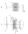
- FIG. 2 is an explanatory diagram illustrating a method of applying a load to the target S without contact.
- A schematically shows the configuration of the load device 13 and its periphery.
- B shows the load state of acoustic radiation pressure.
- the object S is accommodated in a container 80, and the container 80 is set on the support base 70.
- the target S is a regenerated tissue, contamination is not caused during load loading or OCT measurement.
- the container 80 accommodates the substrate 82 seeded with the target S in a state of being immersed in the culture solution C, and is closed (sealed) by a lid 84.
- the container 80, the base material 82, and the lid 84 are made of a material having translucency and sound wave permeability.
- the support base 70 is provided with a vertical through hole 86.
- the container 80 is placed on the support base 70 so as to straddle the through hole 86, and the back surface side is exposed through the through hole 86.
- the object S is arranged so that at least the measurement range is included in the projection plane in the axial direction of the through hole 86.
- the ultrasonic device 72 faces the back surface of the container 80 through the through hole 86 and outputs ultrasonic waves toward the target S.
- the ultrasonic device 72 has a curved transducer array 90 on its upper surface.
- the transducer array 90 includes a plurality of elements 92 arranged in a curved shape.
- the element 92 includes an ultrasonic element (piezo element) that generates ultrasonic waves for vibration.
- the acoustic radiation pressure is focused with the desired position in the target S as the focal point F, and the tissue is focused at the focal point F. It can be vibrated (displaced) (see white arrow).
- a shear wave is generated in the direction parallel to the surface of the object S starting from the focal point F (see a two-dot chain line arrow).
- the light axis by OCT is set to pass through the focal point F of the object S.
- the position of the focal point F can be adjusted (scanned) by selecting (changing) a drive target (energization target) among the plurality of elements 92.
- the ultrasonic radiation elements may be arranged in a planar shape and the acoustic radiation pressure may be focused on the focal point F by using an acoustic lens.
- the control calculation unit 14 sets the focal point F of the acoustic radiation pressure in the target S, the ultrasonic element to be driven, the excitation frequency by the acoustic radiation pressure, and the like, and sends a control signal (pulse) to the drive circuit 74 based on these settings. Output.
- a drive signal (pulse) is output from the drive circuit 74 to the ultrasonic device 72, and an ultrasonic wave (excitation pulse) is output toward the focal point F.
- the control calculation unit 14 can acquire this optical interference signal as a tomographic image of the target S based on the interference light intensity.
- this tomographic distribution can be calculated in three dimensions, the calculation in one or two dimensions will be described here.
- the coherence length l c which is the resolution in the OCT optical axis direction (depth direction) is determined by the autocorrelation function of the light source.
- the coherence length l c is the half-width of the comprehensive line of the autocorrelation function and can be expressed by the following formula (1).
- ⁇ c is the center wavelength of the beam
- ⁇ is the full width at half maximum of the beam.
- the resolution in the direction perpendicular to the optical axis is 1 ⁇ 2 of the beam spot diameter D based on the light condensing performance of the condensing lens.
- the beam spot diameter ⁇ can be expressed by the following formula (2).
- d is a beam diameter incident on the condenser lens
- f is a focal length of the condenser lens.
- the deformation rate distribution of the tissue can be calculated. That is, the electric field E ′ r (t) of the reference light is represented by the following formula (3).
- a (t) is the amplitude
- ⁇ c is the central angular frequency of the light source
- ⁇ r is the Doppler angular frequency generated by the rotation of the RSOD reference mirror 26.
- the electric field E ′ o (t) of the object light is expressed by the following formula (4).
- the detected interference light intensity I ′ d (t) is expressed by the following formula (5).
- the detected tomographic interference signal I d (x, y, z) is expressed by the following equation (6).
- the angular frequency of the interference signal is ⁇ r ⁇ d .
- the Doppler angular frequency shift amount ⁇ d caused by the deformation speed is detected.
- the Doppler angular frequency shift amount omega d it is possible to obtain a deformation speed v.
- lambda c is the center wavelength
- theta (x, y, z) angle formed coordinates (x, y, z) is the incident direction of the deformation rates in the direction of the beam at the light source.
- n is the average refractive index inside the tissue.
- a depth direction (Z-axis direction) scanning method using RSOD is employed.
- the Hilbert transform and the adjacent autocorrelation method are applied. That is, the adjacent autocorrelation method is applied to the analysis signal (complex signal) ⁇ (t) obtained by applying the Hilbert transform to spatially adjacent interference signals.
- the phase difference ⁇ at a predetermined time interval (time difference ⁇ T) in an arbitrary coordinate is obtained, and the Doppler angular frequency shift amount ⁇ d due to the deformation speed is detected.
- the respective interference signals are expressed by the following equation (8).
- s (t) represents the real part of the analytic signal ⁇ (t)
- s ⁇ (t) represents the imaginary part
- ⁇ T represents the acquisition time interval of the j, j + 1-th interference signal
- A represents the amplitude of the interference signal (that is, the backscattering intensity).
- the phase difference between the interference signals is zero.
- the phase difference between the interference signals of ⁇ j and ⁇ j + 1 corresponds to the phase change amount ⁇ d ⁇ T due to Doppler modulation caused by the deformation speed. That is, the Doppler angular frequency shift amount ⁇ d generated by the deformation speed is expressed as the following formula (9).
- the amount of phase change can be detected in the range of ⁇ to ⁇ . Further, by performing an ensemble averaging process on n interference signals according to the following equation (10), the detectability of the Doppler angular frequency shift amount ⁇ d can be improved.
- Doppler angular frequency shift amount omega d obtained as above by substituting the above equation (7) can be calculated deformation velocity v. Based on the deformation speed v, the viscoelasticity of the tissue can be calculated.
- the complex elastic modulus of the viscoelastic body is represented by E * in the following formula (11).
- the real part E ′ of the complex elastic modulus E * corresponds to a component in which stress and strain are in phase
- the imaginary part E ′′ corresponds to a component in which stress and strain are 90 degrees out of phase.
- the former E ′ is an elastic component.
- storage elastic modulus E ′ is an elastic component.
- storage elastic modulus E ′ (hereinafter referred to as “storage elastic modulus E ′”).
- the latter E ′′ corresponds to a viscous component in which the stress and strain rate are in phase and is called “loss elastic modulus” (hereinafter referred to as “loss elastic modulus E” ”). Therefore, the distribution of the storage elastic modulus E ′ and the loss elastic modulus E ′′ can be calculated as a viscoelastic distribution.
- the strain amount (strain rate) at each time can be calculated by the least square method from the distribution of the tissue deformation rate v (distribution in the Z direction), and the amplitude of the strain amount (strain amplitude ⁇ 0) can be detected as a fault.
- the magnitude of the ultrasonic acoustic radiation pressure (stress amplitude ⁇ 0) is a control amount set for the ultrasonic device 72 by the control calculation unit 14, and thus can be grasped.
- the control calculation unit 14 grasps the ultrasonic oscillation timing and the OCT measurement timing, the phase difference (loss angle ⁇ ) between stress and strain can be calculated. Therefore, the storage elastic modulus E ′ and the loss elastic modulus E ′′, which are viscoelastic parameters, can be calculated from the following formula (11), respectively.
- the fault distribution of the storage elastic modulus E ′ and the loss elastic modulus E ′′ obtained in this manner substantially indicates the viscoelastic fault distribution of the tissue.
- the control calculation unit 14 performs the viscoelasticity of the tissue. Visualize the fault.
- This technique is a technique of calculating a deformation vector distribution by applying a digital cross-correlation method to two OCT tomographic images before and after deformation of a measurement object, and detecting a strain rate tensor distribution of the tissue on a micro scale. .
- the recursive cross-correlation method which performs repeated cross-correlation processing.
- This is a technique of applying a cross-correlation method by referring to a deformation vector calculated at a low resolution, limiting an exploration area and hierarchically reducing an inspection area. Thereby, a high-resolution deformation vector can be acquired.
- an adjacent cross-correlation multiplication method (Adjacent cross-correlation Multiplication) that performs multiplication with a correlation value distribution in an adjacent inspection region is used. Then, the maximum correlation value is searched from the correlation value distribution that has been multiplied to increase the SN.
- the sub-pixel accuracy of the deformation vector is important.
- both the up-stream gradient method using brightness gradient (Up-stream Gradientmethod) and the image deformation method considering image expansion and shear (Image Deformation method) are used together to detect deformation vectors with high accuracy.
- the “windward gradient method” here is a kind of gradient method (optical flow method).
- FIG. 3 is a diagram schematically showing a processing procedure by the recursive cross-correlation method.
- FIG. 4 is a diagram schematically showing a processing procedure by subpixel analysis.
- FIGS. 3A to 3C show processing steps by the recursive cross-correlation method. Each figure shows tomographic images before and after continuous imaging by OCT. The previous tomographic image (Image1) is shown on the left side, and the later tomographic image (Image2) is shown on the right side.
- the cross-correlation method is a method for evaluating the local speckle pattern similarity based on the correlation value R ij based on the following equation (12). For this reason, as shown in FIG. 3A, with respect to the preceding and following OCT images, an inspection region S1 to be inspected with similarity to the previous tomographic image (Image1) is set, and the subsequent tomographic image is displayed. In (Image2), a search area S2 that is a search range of similarity is set.
- the Z axis is set in the optical axis direction
- the X axis is set in the direction perpendicular to the optical axis.
- f (X i , Z j ) and g (X i , Z j ) are in the inspection area S1 (N x ⁇ N z pixels) of the center position (X i , Z j ) set in the OCT images before and after the deformation. Represents a speckle pattern. Note that f ⁇ and g ⁇ represent average values of f (X i , Z j ) and g (X i , Z j ) in the inspection region S1.
- a correlation value distribution R i, j ( ⁇ X, ⁇ Z) in the search area S2 (M x ⁇ M z pixels) is calculated, and pattern matching is performed as shown in FIG.
- the movement amount U i, j giving the maximum correlation value is determined as the deformation vector before and after the deformation.
- This method employs a recursive cross-correlation method that increases the spatial resolution by repeating the cross-correlation process while reducing the inspection area S1.
- the spatial resolution is doubled.
- the inspection area S1 is divided into 1 ⁇ 4, and the search area S2 is reduced by referring to the deformation vector calculated in the previous hierarchy.
- the search area S2 is also divided into 1 ⁇ 4.
- Equation (14) is used to set a threshold value using the average deviation ⁇ of a total of nine deformation vectors including the surrounding eight coordinates centered on the coordinates being calculated, and remove the erroneous vectors. Suppresses error propagation associated with recursive processing.
- Um represents the median value of the vector quantity, and the coefficient ⁇ serving as a threshold is arbitrarily set.
- an adjacent cross-correlation multiplication method is introduced as a method for determining an accurate maximum correlation value from a highly random correlation value distribution affected by speckle noise.
- the correlation value distribution Ri, j ( ⁇ x, ⁇ z) in the inspection region S1 and Ri + ⁇ i, j ( ⁇ x, ⁇ z) with respect to the adjacent inspection region overlapping the inspection region S1 Multiplication of Ri, j + ⁇ j ( ⁇ x, ⁇ z) is performed, and a maximum correlation value is retrieved using a new correlation value distribution R′i, j ( ⁇ x, ⁇ z).
- Windward gradient method 4A to 4C show a processing process by subpixel analysis. Each figure shows tomographic images before and after continuous imaging by OCT. The previous tomographic image (Image1) is shown on the left side, and the later tomographic image (Image2) is shown on the right side.
- an upwind gradient method and an image deformation method are used for subpixel analysis.
- the final movement amount is calculated by an image deformation method described later
- the windward gradient method is applied prior to the image deformation method because of the problem of convergence of the calculation.
- the image deformation method and the windward gradient method for detecting the sub-pixel movement amount with high accuracy are applied under the condition of the inspection area size being small and the high spatial resolution.
- the subpixel movement amount is calculated by the windward gradient method.
- the luminance difference before and after deformation at the point of interest is represented by the luminance gradient and movement amount of each component.
- the sub-pixel movement amount can be determined using the least square method from the luminance gradient data in the inspection region S1.
- the windward difference method is used which gives the windward brightness gradient before the subpixel deformation.
- the windward gradient method calculates the movement of the point of interest in the inspection region S1 not only with the pixel accuracy shown in FIG. 4A but also with the sub-pixel accuracy shown in FIG. 4B.
- Each grid in the figure represents one pixel. Actually, it is considerably smaller than the tomographic image shown in the figure, but for the convenience of explanation, it is shown in large size.
- This windward gradient method is a method for formulating the change of the luminance distribution before and after the minute deformation by the luminance gradient and the moving amount.
- f is the luminance
- the following equation (Taylor expansion of the minute deformation f (x + ⁇ x, z + ⁇ z) is performed. 16).
- the above formula (16) indicates that the luminance difference before and after the deformation of the attention point is represented by the luminance gradient and the movement amount before the deformation. Since the movement amount ( ⁇ x, ⁇ z) cannot be determined only by the above equation (16), it is assumed that the movement amount is constant in the inspection region S1, and is calculated by applying the least square method.
- the luminance difference before and after the movement at each point of interest on the right side can only be obtained uniquely. Therefore, how accurately the luminance gradient is calculated is directly related to the accuracy of the movement amount.
- the primary accuracy upwind difference is used. This is because applying high-order differences in differentiating requires a lot of data and is greatly affected when noise is included.
- the high-order difference based on each point in the inspection area S1 uses a lot of data outside the inspection area S1, and there is a problem that the amount of movement of the inspection area S1 itself is lost. is there.
- the difference on the windward side is applied before the deformation.
- the windward is not the actual movement direction but the direction of the subpixel movement amount with respect to the pixel movement amount, and the upwind is determined by performing parabolic approximation on the maximum correlation value peak.
- the luminance difference on the leeward side after the deformation moves in the opposite direction, a difference in luminance at the point of interest occurs, so the difference on the leeward side is applied after the deformation.
- the position of the point of interest before (after) deformation is obtained from the amount of subpixel movement when parabolic approximation is performed.
- the luminance gradient is calculated from the ratio thereof. Specifically, the following formula (17) is used.
- the amount of movement was determined by applying the least square method using the luminance gradient thus calculated and the luminance change.
- the cross-correlation is performed between the inspection region S1 before the tissue deformation and the inspection region S1 in consideration of the expansion and contraction and shear deformation after the tissue deformation, and the sub-pixel deformation amount is determined by iterative calculation based on the correlation value. Note that the expansion and contraction and the shear deformation of the inspection region S1 are linearly approximated.
- the image deformation method is generally used in a material surface strain measurement method, and is applied to an image obtained by photographing a material surface coated with a random pattern with a high spatial resolution camera.
- the OCT tomogram not only contains a lot of speckle noise, but especially in a living tissue, the refractive index changes with the flow of the substrate and water in the tissue, so the deformation to the speckle pattern is large.
- Reduction of the examination area S1 in this method is indispensable for detecting local tissue mechanical characteristics.
- the amount of deformation obtained by the windward gradient method is adopted as the initial value of the convergence calculation, and further, low robustness is realized even when the inspection area S1 is reduced by bicubic function interpolation of the luminance distribution. ing.
- an interpolation function other than bicubic function interpolation may be used.
- a bicubic function interpolation method is applied to the luminance distribution of the OCT tomogram before tissue deformation, and the luminance distribution is made continuous.
- the bicubic function interpolation method is a technique for reproducing spatial continuity of luminance information using a convolution function obtained by piecewise approximating a sinc function.
- a point spread function depending on the optical system is convolved. Therefore, by performing deconvolution using a sinc function, the original continuous luminance distribution is restored.
- the convolution function h (x) is expressed by the following equation (18).
- the value of a is determined based on the verification result by the numerical experiment using the pseudo OCT tomogram.
- the inspection region S1 calculated in consideration of expansion and contraction and shear deformation is accompanied by deformation as it moves.
- the values of x * , z * Is represented by the following formula (19).
- ⁇ x and ⁇ z are distances from the center of the inspection region S1 to the coordinates x and z
- u and v are deformation amounts in the x and z directions, respectively
- ⁇ u / ⁇ x and ⁇ v / ⁇ z are x, respectively.
- the deformation amount in the vertical direction of the inspection region S1 in the z direction, ⁇ u / ⁇ z, and ⁇ v / ⁇ x are the deformation amounts in the shear direction of the inspection region S1 in the x and z directions, respectively.
- the Newton-Raphson method is used for the numerical solution, and the correlation value derivative with 6 variables (u, v, ⁇ u / ⁇ x, ⁇ u / ⁇ z, ⁇ v / ⁇ x, ⁇ v / ⁇ z) is 0. That is, iterative calculation is performed so as to obtain the maximum correlation value.
- the sub-pixel movement amount obtained by the windward gradient method is used as the initial movement amount in the x and z directions.
- the Hessian matrix for the correlation value R is H and the Jacobian vector for the correlation value is ⁇ R
- the update amount ⁇ Pi obtained in one iteration is expressed by the following equation (20).
- the asymptotic solution obtained at any time by iterative calculation is sufficiently small in the vicinity of the convergence solution.
- a correct convergence solution may not be obtained because it cannot be followed by linear deformation.
- the sub-pixel movement amount obtained by the windward gradient method is employed.
- the deformation velocity vector distribution can be calculated by differentiating the deformation vector of subpixel accuracy obtained in this way with respect to time.
- MLSM Moving least square method
- MLSM is a technique that enables smooth calculation of a differential coefficient while smoothing a movement amount distribution.
- the square error equation used in MLSM is expressed by the following equation (21).
- Equation (21) parameters a to k that minimize S (x, z, t) are obtained. That is, the following equation (22) is adopted as a three-variable quadratic polynomial in the horizontal direction x, the depth direction z, and the time direction t as an approximate function. Based on the least square approximation, an optimal derivative is calculated from the following equation (23) and smoothed.
- the strain rate tensor shown in the following formula (24) can be calculated.
- fx and fz indicate the strain increment of each axis, and the strain rate is calculated from the amount of change over time.
- the strain amount can be calculated by time integration of the strain rate calculated by the above equation (24), and the amplitude of the strain amount (strain amplitude ⁇ 0) can be detected as a fault. Further, as described in relation to the above equation (11), the magnitude of the ultrasonic acoustic radiation pressure (stress amplitude ⁇ 0) can be given as the modulation amplitude by the control calculation unit 14 or the drive circuit 74. It is known and the phase difference (loss angle ⁇ ) between stress and strain can also be calculated. Therefore, the storage elastic modulus E ′ and the loss elastic modulus E ′′, which are viscoelastic parameters, can be calculated.
- the fault distribution of the storage elastic modulus E ′ and the loss elastic modulus E ′′ obtained in this way is the viscoelasticity parameter of the tissue.
- the fault distribution will be substantially shown.
- the control calculation unit 14 visualizes the viscoelasticity of the tissue as a tomogram. In addition, formulation is possible even with the strain rate. That is, correspondence with viscoelastic parameters can be taken.
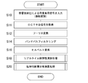
- FIG. 5 is a flowchart showing the flow of the viscoelastic tomographic visualization process executed by the control calculation unit 14. This process is repeatedly executed at a predetermined calculation cycle.
- the control calculation unit 14 drives and controls the light source 2, the optical mechanisms 8 and 10, and the load device 13. Thereby, the acoustic radiation pressure load signal appropriately amplitude-modulated is input to the tissue (S10), and an optical interference signal by OCT is acquired (S11).
- the control calculation unit 14 performs frequency analysis by performing Fourier transform on the optical interference signal for calculation in the frequency space (S12). Subsequently, after the band-pass filtering process is executed so as to correspond to the modulation frequency in the optical mechanism 10 to improve the signal SN ratio (S14), the Hilbert transform is executed (S16). An autocorrelation type real-time viscoelasticity calculation process is executed using the analysis signal obtained by the Hilbert transform (S18). In parallel with this, viscoelastic fault distribution calculation processing is executed (S20).
- the real-time viscoelasticity calculation process is a process of calculating and visualizing the uniaxial (Z direction) viscoelasticity in the tissue of the target S almost in real time in the process of acquiring the OCT tomographic image.
- the viscoelastic tomographic distribution calculation process is a process of acquiring a plurality of OCT tomographic images (two-dimensional images) and visualizing the viscoelasticity of the tissue in a post-process based on them.
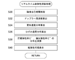
- FIG. 6 is a flowchart showing in detail the real-time viscoelasticity calculation process of S18 in FIG.
- the control calculation unit 14 performs adjacent autocorrelation processing using the analysis signal acquired in S16 to obtain a phase difference at an arbitrary coordinate (S30), and obtains a Doppler frequency (Doppler angular frequency shift amount) (S32).
- the tomographic distribution of the deformation speed in the tissue is calculated by spatial smoothing or spatial averaging processing (S34).
- a strain distribution strain rate distribution
- S36 the least squares method
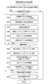
- FIG. 7 is a flowchart showing in detail the viscoelastic fault distribution calculation process of S20 in FIG.
- the control calculation unit 14 calculates the interference light intensity based on the envelope (amplitude) of the analysis signal (S50).
- S50 envelope
- I amplitude
- Is read (S54).
- processing by a recursive cross correlation method is executed.
- cross-correlation processing is executed at the minimum resolution (inspection area of the maximum size) to obtain a correlation coefficient distribution (S56).
- the product of adjacent correlation coefficient distributions is calculated by the adjacent cross correlation multiplication method (S58).
- error vectors are removed by a spatial filter such as a standard deviation filter (S60), and interpolation of the removal vectors is executed by a least square method or the like (S62).
- the cross correlation process is continued by increasing the resolution by reducing the inspection area (S64). That is, the cross-correlation process is executed based on the reference vector at the low resolution. If the resolution at this time is not the predetermined maximum resolution (N in S66), the process returns to S58.
- the processing from S58 to S66 is repeated, and when the cross-correlation processing at the highest resolution is completed (Y in S66), the sub-pixel analysis is executed. That is, based on the distribution of the deformation vector at the maximum resolution (the inspection area of the minimum size), the subpixel movement amount by the windward gradient method is calculated (S68). Based on the sub-pixel movement amount calculated at this time, the sub-pixel deformation amount by the image deformation method is calculated (S70). Subsequently, the error vector is removed by filtering using the maximum cross-correlation value (S72), and interpolation of the removal vector is executed by the least square method or the like (S74).
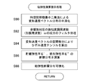
- FIG. 8 is a flowchart showing in detail the viscoelasticity calculation presentation process of S80 in FIG.
- the control calculation unit 6 executes the smoothing of the deformation velocity vector distribution calculated in S76 by the space-time moving least square method (S90). Then, only the component synchronized with the excitation frequency ⁇ (amplitude modulation frequency) by the acoustic radiation pressure is extracted from the smoothed deformation velocity vector (S92). Then, the strain rate tensor is calculated by performing spatial differentiation on the deformation rate vector (S94).
- the strain rate is calculated by time-integrating the strain rate obtained in S94, and the fault distribution of the strain amount (strain amplitude ⁇ 0) is calculated.
- a fault having a storage elastic modulus E ′ and a loss elastic modulus E ′′ using the magnitude of the acoustic radiation pressure of ultrasonic waves (stress amplitude ⁇ 0) and the phase difference between stress and strain (loss angle ⁇ ).
- the distribution is calculated (S96), and the viscoelasticity of the tissue is visualized as a tomogram (S98) It is possible to formulate even with the strain rate, that is, the correspondence with the viscoelastic parameters can be taken.
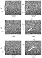
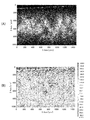
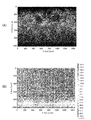
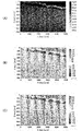
- FIG. 9 and FIG. 10 are diagrams showing experimental results for a sample simulating a biological tissue.
- FIG. 9 shows the results when a hard gel sample is used
- FIG. 10 shows the results when a soft gel sample is used.
- (A) shows an OCT tomographic image
- (B) shows a tomographic distribution of deformation speed (see the above equation (7)).
- the deflection angle of the reference mirror 26 was set to ⁇ 1.9 deg, the scanning frequency was set to 4 kHz, and the depth scanning range (Z direction detection range) of the sample was set to 900 ⁇ m.
- the ultrasonic device 72 was driven with a fundamental wave of 1 MHz, and the applied sound pressure was measured with a hydrophone before the experiment.
- a gel sample (15 mm ⁇ 15 mm ⁇ 5 mm) simulating the optical characteristics of human skin was used.
- Two types of gel samples were prepared: a soft gel sample with a gel hardener weight percentage of 0.5% and a hard gel sample with a weight percentage of the gel hardener four times that of the gel hardener. Visualization evaluation was performed.
- the deformation rate is small in the high-rigid hard gel sample and the deformation rate is large in the low-rigid soft gel sample. This can be said to be in line with the actual situation that the low rigidity portion of the living tissue vibrates greatly (large amplitude) and the high rigidity portion vibrates small (small amplitude) with respect to the excitation force.
- the distribution of the deformation speed in the soft gel sample is due to the distribution of the acoustic radiation pressure.
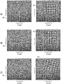
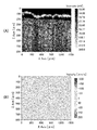
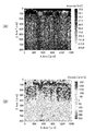
- FIG. 11 and FIG. 12 are diagrams showing experimental results for a layered sample in which the rigidity is changed to a layer.
- FIG. 11 shows the experimental results when no acoustic radiation pressure is applied
- FIG. 12 shows the experimental results when the acoustic radiation pressure is applied.
- (A) shows an OCT tomogram
- (B) shows a tomographic distribution of deformation speed.
- a soft gel layer was used up to about 200 ⁇ m from the surface, and a hard gel layer was used up to about 1000 ⁇ m below it.
- FIG. 13 is a diagram illustrating experimental results related to viscosity evaluation.
- A shows an OCT tomogram
- B shows a tomographic distribution of deformation speed.
- C shows that there is a phase lag of the deformation speed in the depth direction (Z direction) in (B) by a two-dot chain line.
- a sample similar to that shown in FIG. 12 was used. While performing X-direction scanning in OCT, the amplitude of the acoustic radiation pressure due to ultrasonic waves was periodically changed, and the resulting deformation speed was visualized as a tomogram.
- the amplitude modulation frequency is 2.4 Hz.
- the micro-tomography of the viscoelasticity of the tissue of the target S is visualized by non-contact load loading by acoustic radiation pressure and non-contact / non-invasive tomographic measurement by OCT. For this reason, even if the target S requires strict quality assurance, the contamination can be prevented and the mechanical property evaluation can be performed with high accuracy. This is considered to contribute to the elucidation of biomechanics of regenerative tissues.
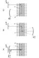
- FIG. 14 is a diagram illustrating a load application method according to a modification.
- A shows a 1st modification
- B shows a 2nd modification
- C shows a 3rd modification.
- the optical mechanism 8 and the ultrasonic device 172 are set on the same side with respect to the target S, and the optical axis by OCT is set to pass through the focal point F.
- the transducer array 190 is formed in a donut shape, and a hole 192 is formed in the center thereof.
- the OCT light is applied to the object S through the hole 192. According to such a structure, it is not necessary to provide a through-hole like the said Example in the support stand of a load apparatus.
- the optical mechanism 8 and the ultrasonic device 72 are arranged on the opposite side with respect to the target S, and the optical axis does not pass through the focus F in the process of tomographic measurement by OCT.
- the case where the focal point F of the ultrasonic device 72 is fixed and OCT X-direction scanning is performed corresponds to this case.
- the deformation of the tissue at a position displaced from the focal point F in the X direction by a predetermined distance is detected.
- the optical mechanism 8 and the ultrasonic device 72 are arranged on the same side with respect to the target S, and the optical axis is set so as not to pass the focal point F in the process of tomographic measurement by OCT. .
- the amplitude and phase of the acoustic radiation pressure can be easily grasped at the detection location by OCT, so that the arithmetic processing becomes easy.
- the accuracy is easy to increase.
- the second and third modified examples have an advantage that the system can be easily constructed.
- the viscoelasticity of the tissue may be determined based on the propagation speed. That is, non-contact elastography based on acoustic radiation pressure may be used to detect tissue viscoelasticity by OCT.
- the support base 70 is fixed, and the optical axis of the OCT and the focal point of the ultrasonic wave are moved.
- the support base 70 may be controlled to move in the X direction and the Y direction, and the ultrasonic focus and the OCT detection position in the target S may be changed.
- the measurement target is a regenerative tissue (cultured cell)
- the above apparatus may be applied to a regenerative treatment of a living body and tissue engraftment may be monitored.
- the apparatus can be applied not only to the medical field such as cartilage diagnosis and skin diagnosis but also to various uses and fields such as the cosmetic surgery field and the cosmetic industry field.
- tissue deformation is induced by acoustic radiation pressure.
- tissue deformation may be induced by incorporating particles having electrical conductivity or magnetism (such as molecular target drugs) into a living tissue and irradiating an electromagnetic field.
- viscoelasticity evaluation is performed from the storage elastic modulus E ′ and the loss elastic modulus E ′′ is shown, but a value expressing the viscoelastic physical quantity is newly added from the storage elastic modulus E ′ and the loss elastic modulus E ′′.
- viscoelasticity evaluation may be performed based on the definition.
- a tomographic image by OCT is acquired in two dimensions, but it may be acquired in three dimensions. That is, not only the depth direction (Z direction) and the X direction but also the Y direction may be scanned to visualize the viscoelasticity of the tissue as a tomographic image.
- this invention is not limited to the said Example and modification, A component can be deform
- Various inventions may be formed by appropriately combining a plurality of constituent elements disclosed in the above-described embodiments and modifications. Moreover, you may delete some components from all the components shown by the said Example and modification.
Landscapes
- Health & Medical Sciences (AREA)
- Life Sciences & Earth Sciences (AREA)
- Physics & Mathematics (AREA)
- General Health & Medical Sciences (AREA)
- Pathology (AREA)
- Radiology & Medical Imaging (AREA)
- Nuclear Medicine, Radiotherapy & Molecular Imaging (AREA)
- General Physics & Mathematics (AREA)
- Surgery (AREA)
- Heart & Thoracic Surgery (AREA)
- Medical Informatics (AREA)
- Veterinary Medicine (AREA)
- Public Health (AREA)
- Animal Behavior & Ethology (AREA)
- Molecular Biology (AREA)
- Biophysics (AREA)
- Engineering & Computer Science (AREA)
- Biomedical Technology (AREA)
- Chemical & Material Sciences (AREA)
- Immunology (AREA)
- Analytical Chemistry (AREA)
- Biochemistry (AREA)
- Acoustics & Sound (AREA)
- Optics & Photonics (AREA)
- Dermatology (AREA)
- Investigating Or Analysing Materials By Optical Means (AREA)
Abstract
ある態様の装置1は、OCTを用いる光学系を含み、対象Sにおける組織の粘弾性を断層可視化する。この装置は、光源2からの光を対象Sの組織に導いて走査させるための光学機構8と、組織に対して変形エネルギーを付与するための負荷装置13と、負荷装置13および光学機構8の駆動を制御し、それらの駆動に基づいて上記光学系による光干渉信号を処理することにより、組織の粘弾性の断層分布を演算する制御演算部14と、組織の粘弾性を断層可視化する態様で表示する表示装置16と、を備える。負荷装置13は、対象Sの内部に設定された焦点に向けて超音波を出力することにより、組織に対して音響放射圧を負荷する非接触負荷装置である。
Description
本発明は、測定対象の組織の粘弾性をマイクロスケールにて断層表示可能な装置および方法に関する。
近年、医療診断技術の更なる発展に向けて光干渉断層画像法(Optical Coherence Tomography:以下「OCT」という)の臨床応用が進められている。OCTは、低コヒーレンス光干渉を利用した断層画像法であり、マイクロスケールの高空間分解能にて生体組織の形態分布を可視化できる。また、2次元OCTの取得レートはビデオレート以上であり、高時間分解能も有している。
そこで、発明者らは、OCTを用いて生体組織の力学特性を断層可視化する手法を提案している(特許文献1)。軟骨や皮膚等の生体組織では基質量の変化よりも組織の力学特性の変化が有意に現れるため、組織内部のマイクロバイオメカニクスの定量評価が診断技術の向上に寄与すると考えたものである。本手法は、生体組織の特性(粘弾性)を評価可能なOCTシステムの開発を目指したものである。
ところで、このような力学特性評価を行う場合、OCT計測に際して生体組織を変形させるアルゴリズムが組み込まれる。そのため、特許文献1の技術では、圧電素子を測定対象の表面に接触させて負荷する方法を採用している。しかし、例えば再生組織など、厳格な品質保証を要する測定対象を扱う場合、このような圧電素子の接触が組織の汚染を招き、システムの実用化を妨げるおそれがある。発明者は、このような知見のもと、上記OCTシステムの改善が必要であるとの認識に到った。
本発明はこのような課題に鑑みてなされたものであり、その目的の一つは、厳格な品質保証を要する測定対象に対しても、OCT計測による力学特性評価を可能とする技術を提供することにある。
本発明のある態様は、OCTを用いる光学系を含み、測定対象における組織の粘弾性を断層可視化する粘弾性可視化装置に関する。この装置は、光源からの光を組織に導いて走査させるための光学機構と、組織に対して変形エネルギーを付与するための負荷装置と、負荷装置および光学機構の駆動を制御し、それらの駆動に基づいて光学系による光干渉信号を処理することにより、組織の粘弾性の断層分布を演算する制御演算部と、組織の粘弾性を断層可視化する態様で表示する表示装置と、を備える。負荷装置は、測定対象の内部に設定された焦点に向けて超音波を出力することにより、組織に対して音響放射圧による加振力を負荷する非接触負荷装置である。
本発明の別の態様は、測定対象の組織の粘弾性を断層可視化する粘弾性可視化方法に関する。この方法は、組織に対して超音波の音響放射圧にて荷重を負荷する負荷工程と、OCTを用いることにより、荷重の負荷により変形する組織からの後方散乱光に基づく光干渉信号を取得する干渉信号取得工程と、光干渉信号を処理し、組織の変形に伴う所定の力学特徴量の変化に基づいて組織の粘弾性の断層分布を演算する演算工程と、組織の粘弾性を断層可視化する表示工程と、を備える。
本発明によれば、品質保証を要する測定対象に対しても、OCT計測による力学特性評価を可能とする技術を提供できる。
本発明の一実施形態は、OCTを用いる粘弾性可視化装置である。この装置は、光源、光学機構、負荷装置、制御演算部および表示装置を備え、測定対象における組織の粘弾性を断層可視化する。「測定対象」は、皮膚や軟骨等の生体組織であってもよいし、再生皮膚や再生軟骨等の再生組織(培養細胞からなる組織)であってもよい。負荷装置は、測定対象の内部に設定される焦点に向けて超音波を出力し、組織に対して音響放射圧を負荷する。焦点は、測定対象の内部において音響放射圧による加振力が集中するポイントであり、制御演算部により設定される。
この態様では、組織の粘弾性を断層可視化するために、音響放射圧による負荷とOCTによる検出が行われる。音響放射圧による負荷は、動的荷重(加振力)であってよい。音響放射圧により測定対象の所望の断層位置に非接触にて荷重を付与し、組織変形を誘発できる。また、OCTにより非接触・非侵襲にて断層計測が可能となる。すなわち、この態様によれば、負荷装置および光学機構の双方を測定対象に対して非接触とすることができる。このため、測定対象が厳格な品質保証を要するものであったとしても、その汚染を防止でき、力学特性(粘弾性)を評価できる。
測定対象に向けて照射される光の軸が、測定対象における音響放射圧の焦点を通るように設定されてもよい。それにより、その焦点位置にある組織の変形をダイレクトかつリアルタイムに検出できる。あるいは、その光軸を焦点から所定距離の位置に設定し、その距離に応じた粘弾性の評価基準を設定してもよい。
制御演算部は、組織の変形によって生じる所定の力学特徴量、又は組織の変形に伴う力学特徴量の変化を測定対象の断層位置に対応づけて演算し、その演算結果に基づいて組織の粘弾性の断層分布を演算してもよい。ここでいう「力学特徴量」は、組織の変形量や変形ベクトルに基づいて得られるものでよい。例えば、変形ベクトルを空間微分したひずみテンソルであってもよい。ひずみの振幅や位相であってもよい。あるいは、変形ベクトルを時間微分した変形速度ベクトルであってもよいし、変形速度ベクトルをさらに空間微分したひずみ速度テンソルであってもよい。それらの振幅や位相であってもよい。音響放射圧による加振力の振幅と、OCTにより検出されるひずみの振幅と、それらの位相差とに基づき、粘弾性を算出してもよい。音響放射圧による加振力が負荷装置の駆動により生成されるものであるため、その加振力の振幅および位相が既知であることを利用できる。
負荷変動に対する、変形速度(ひずみ速度)の変動の大きさ(振幅値)と、加振力の変動に対する変形速度(ひずみ速度)の変動の追従性(応答性)が、組織の粘弾性に対応して変化する傾向がある。具体的には、粘性が低下するほど、変形速度(ひずみ速度)の振幅値は大きくなり、時間遅れ(位相遅れ)は小さくなる傾向にある。このような傾向に基づいて粘弾性を評価することもできる。
あるいは、測定対象への超音波の印可によって発生する剪断波を断層検出し、その伝播速度から組織の粘弾性を演算してもよい。音響放射圧による非接触エラストグラフィーを利用し、組織の粘弾性をOCTにより検出するものである。
より具体的には、光学機構が測定対象の表面側から光を照射し、負荷装置が測定対象の裏面側から超音波を出力する構成としてもよい。それにより、光学機構と負荷装置との物理的な干渉を防止し易くなり、装置の設計が容易となる。
このような構成において再生組織を測定対象とする場合、その再生組織を収容する容器を支持する支持台を設けてもよい。この容器として透光性および音波透過性を有するものを採用し、支持台にはその容器の裏面側を露出させるための孔を設けてもよい。それにより、測定対象の表面側から光を受け入れ、裏面側から超音波を受け入れることができる。再生組織の品質保証のため、この容器は密閉可能であることが好ましい。支持台をクリーンベンチ内に配置してもよい。
この装置は、第1光学機構、第2光学機構および光検出装置を備えてもよい。第1光学機構は、測定対象を経由するオブジェクトアームに設けられ、光源からの光を測定対象に導いて走査させる。第2光学機構は、測定対象を経由しないリファレンスアームに設けられ、光源からの光を参照鏡に導いて反射させる。光検出装置は、測定対象にて反射した物体光と参照鏡にて反射した参照光とが重畳された干渉光を検出する。制御演算部は、光検出装置から入力された光干渉信号に対して周波数解析を実行し、ドップラー周波数を用いて組織の変形速度を算出する。そして、その変形速度に基づいて得られるひずみ情報と、前記負荷装置による音響放射圧情報とに基づいて粘弾性を演算してもよい。
以下、図面を参照しつつ、本実施形態を具体化した実施例について詳細に説明する。
[実施例]
図1は、実施例に係る粘弾性可視化装置の構成を概略的に表す図である。本実施例の装置は、再生組織の粘弾性をマイクロスケールにて断層計測し、可視化する。この断層計測のために、音響放射圧による荷重負荷とOCTによる検出を利用する。
[実施例]
図1は、実施例に係る粘弾性可視化装置の構成を概略的に表す図である。本実施例の装置は、再生組織の粘弾性をマイクロスケールにて断層計測し、可視化する。この断層計測のために、音響放射圧による荷重負荷とOCTによる検出を利用する。
図1に示すように、OCT装置1は、光源2、オブジェクトアーム4、リファレンスアーム6、光学機構8,10、光検出装置12、負荷装置13、制御演算部14および表示装置16を備える。各光学要素は、光ファイバにて互いに接続されている。なお、図示の例では、マッハツェンダー干渉計をベースとした光学系が示されているが、マイケルソン干渉計その他の光学系を採用することもできる。また、本実施例では、OCTとしてTD-OCT(Time Domain OCT)を用いるが、SS-OCT(Swept Source OCT)、SD-OCT(Spectral Domain OCT)その他のOCTを用いてもよい。
光源2から出射された光は、カプラー18(ビームスプリッタ)にて分けられ、その一方がオブジェクトアーム4に導かれて物体光となり、他方がリファレンスアーム6に導かれて参照光となる。オブジェクトアーム4の物体光は、サーキュレータ20を介して光学機構8に導かれ、測定対象(以下、「対象S」という)に照射される。対象Sは、本実施例では再生組織(培養組織)である。この物体光は、対象Sの表面および断面にて後方散乱光として反射されてサーキュレータ20に戻り、カプラー22に導かれる。
一方、リファレンスアーム6の参照光は、サーキュレータ24を介して光学機構10に導かれる。この参照光は、光学機構10の参照鏡26にて反射されてサーキュレータ24に戻り、カプラー22に導かれる。すなわち、物体光と参照光とがカプラー22にて合波(重畳)され、その干渉光が光検出装置12により検出される。光検出装置12は、これを光干渉信号(干渉光強度を示す信号)として検出する。この光干渉信号は、A/D変換器28を介して制御演算部14に入力される。
制御演算部14は、光学系全体の制御と、負荷装置(超音波加振装置)の制御と、OCTによる画像出力のための演算処理を行う。制御演算部14の指令信号は、図示略のD/A変換器を介して光源2、光学機構8,10、負荷装置13等に入力される。制御演算部14は、光検出装置12に入力された光干渉信号を処理し、OCTによる対象Sの断層画像を取得する。そして、その断層画像データに基づき、後述の手法により対象Sにおける粘弾性の断層分布を演算する。
より詳細には以下のとおりである。
光源2は、スーパールミネッセントダイオード(Super Luminessent Diode:以下「SLD」と表記する)からなる広帯域光源である。光源2から出射された光は、カプラー18にて物体光と参照光に分けられ、それぞれオブジェクトアーム4、リファレンスアーム6に導かれる。オブジェクトアーム4およびリファレンスアーム6には光ファイバとして、偏光による影響を抑えることが可能な偏波保持光ファイバ(Polarization Maintaining Fiber)が用いられている。
光源2は、スーパールミネッセントダイオード(Super Luminessent Diode:以下「SLD」と表記する)からなる広帯域光源である。光源2から出射された光は、カプラー18にて物体光と参照光に分けられ、それぞれオブジェクトアーム4、リファレンスアーム6に導かれる。オブジェクトアーム4およびリファレンスアーム6には光ファイバとして、偏光による影響を抑えることが可能な偏波保持光ファイバ(Polarization Maintaining Fiber)が用いられている。
光学機構8は、オブジェクトアーム4を構成し、光源2からの光を対象Sに導いて走査させる機構と、その機構を駆動するための駆動部を備える。光学機構8は、コリメータレンズ40、2軸のガルバノミラー42、および対物レンズ44を含む。対物レンズ44は、対象Sに対向配置される。サーキュレータ20を経た光は、コリメータレンズ40を介してガルバノミラー42に導かれ、x軸方向やy軸方向に走査されて対象Sに照射される。対象Sからの反射光は、物体光としてサーキュレータ20に戻り、カプラー22に導かれる。
光学機構10は、RSOD方式(Rapid Scanning Optical Delay Line)の機構であり、リファレンスアーム6を構成する。このRSODは、光が後述の回折格子52に往復1回ずつ照射されるシングルパス型でもよいし、往復2回ずつ照射されるダブルパス型でもよい。光学機構10は、コリメータレンズ50、回折格子52、レンズ54および参照鏡26を含む。サーキュレータ24を経た光は、コリメータレンズ50を介して回折格子52に導かれる。この光は、回折格子52によって波長ごとに分光され、それぞれレンズ54によって参照鏡26上の異なる位置に集光される。参照鏡26を微小角にて回転させることで、高速光路走査および周波数変調が可能となる。参照鏡26からの反射光は、参照光としてサーキュレータ24に戻り、カプラー22に導かれる。そして、物体光と重畳されて干渉光として光検出装置12に送られる。なお、変形例においては、回折格子52を経た光をレンズ54に代えて湾曲ミラーによって参照鏡26に集光してもよい。
光検出装置12は、光検出器60、フィルタ62およびアンプ64を含む。カプラー22を経ることで得られた干渉光は、光検出器60にて光干渉信号として検出される。この光干渉信号は、フィルタ62によりノイズが除去又は低減され、アンプ64およびA/D変換器28を経て制御演算部14に入力される。
負荷装置13は、OCTの光軸上に対象Sを保持するための支持台70、対象Sに向けて超音波を出力する超音波デバイス72、および超音波デバイス72を駆動する駆動回路74を含む。超音波デバイス72の駆動(発振)により、対象Sの内部に向けて超音波ビームが出力される。駆動回路74は、制御演算部14からの指令に基づき、OCTの検出と同期させるようにその超音波ビームを縦横に走査させる。それにより、対象Sの組織の任意位置に非接触にて音響放射圧による動的荷重(振動荷重、加振力)を負荷できる。この発振による音響放射圧負荷信号は、振幅変調させておく必要がある。ここでは、音響放射圧の音圧量(圧縮荷重量)に直接依存する振幅を正弦波で変調して送信する。この振幅変調にて組織の変形が促されるため、この変調による変形速度をOCTにより検出する。
制御演算部14は、CPU、ROM、RAM、ハードディスクなどを有する。制御演算部14は、これらのハードウェアおよびソフトウェアによって、光学系全体の制御と、負荷装置13の駆動制御と、OCTによる画像出力のための演算処理を行う。制御演算部14は、負荷装置13および光学機構8,10の駆動を制御し、それらの駆動に基づいて光検出装置12から出力された光干渉信号を処理し、OCTによる対象Sの断層画像を取得する。そして、その断層画像データに基づき、後述の手法により対象Sにおける組織の粘弾性を演算する。
表示装置16は、例えば液晶ディスプレイからなり、制御演算部14にて演算された対象Sの組織の粘弾性を断層可視化する態様で画面に表示する。
図2は、対象Sに非接触にて荷重負荷を行う方法を表す説明図である。(A)は、負荷装置13およびその周辺の構成を模式的に示す。(B)は、音響放射圧の負荷状態を示す。
図2(A)に示すように、対象Sは容器80に収容され、その容器80が支持台70にセットされる。本実施形態では、対象Sが再生組織であるため、荷重負荷やOCT計測に際して汚染を生じさせないようにするものである。容器80は、対象Sが播種された基材82を培養液Cに浸した状態で収容し、蓋84により閉止(密閉)されている。容器80,基材82および蓋84は、透光性および音波透過性を有する材質からなる。なお、光学機構8および負荷装置13の少なくとも一部をクリーンベンチ内に収容し、容器80内への塵埃や雑菌の混入を確実に防止できるのが好ましい。
図2(A)に示すように、対象Sは容器80に収容され、その容器80が支持台70にセットされる。本実施形態では、対象Sが再生組織であるため、荷重負荷やOCT計測に際して汚染を生じさせないようにするものである。容器80は、対象Sが播種された基材82を培養液Cに浸した状態で収容し、蓋84により閉止(密閉)されている。容器80,基材82および蓋84は、透光性および音波透過性を有する材質からなる。なお、光学機構8および負荷装置13の少なくとも一部をクリーンベンチ内に収容し、容器80内への塵埃や雑菌の混入を確実に防止できるのが好ましい。
支持台70には、上下方向の貫通孔86が設けられている。容器80は、貫通孔86を跨ぐように支持台70に載置され、その貫通孔86を介して裏面側を露出させる。対象Sは、少なくともその計測範囲が貫通孔86の軸線方向の投影面に含まれるように配置される。超音波デバイス72は、貫通孔86を介して容器80の裏面に対向し、対象Sに向けて超音波を出力する。
超音波デバイス72は、その上面に曲面状の振動子アレイ90を有する。振動子アレイ90は、曲面状に配置された複数の素子92を有する。素子92は、加振用の超音波を発生させる超音波素子(ピエゾ素子)からなる。図2(B)にも示すように、各素子92からの超音波の出力を調整することにより、対象S内の所望位置を焦点Fとして音響放射圧を集束させ、その焦点Fにて組織を加振する(変位させる)ことができる(白抜き矢印参照)。この音響放射圧の生成によって、焦点Fを起点として対象Sの表面と平行な方向にせん断波が発生する(二点鎖線矢印参照)。本実施例では、OCTによる光の軸が、対象Sの焦点Fを通るように設定される。焦点Fの位置は、複数の素子92のうち駆動対象(通電対象)を選択する(変化させる)ことで調整(走査)できる。なお、変形例においては、超音波素子を平面状等に配置し、音響レンズを用いることで音響放射圧を焦点Fに集束させてもよい。
制御演算部14は、対象Sにおける音響放射圧の焦点F、駆動する超音波素子、音響放射圧による加振周波数等を設定し、これらの設定に基づいて駆動回路74へ制御信号(パルス)を出力する。それにより、駆動回路74から超音波デバイス72へ駆動信号(パルス)が出力され、焦点Fに向けて超音波(加振パルス)が出力される。
以下、対象Sの粘弾性の演算処理方法について詳細に説明する。
上述のように、OCTにおいて、オブジェクトアーム4を経た物体光(測定対象からの反射光)と、リファレンスアーム6を経た参照光とが合波され、光検出装置12により光干渉信号として検出される。制御演算部14は、この光干渉信号を干渉光強度に基づく対象Sの断層画像として取得することができる。この断層分布は三次元で演算することもできるが、ここでは一次元又は二次元での演算について説明する。
上述のように、OCTにおいて、オブジェクトアーム4を経た物体光(測定対象からの反射光)と、リファレンスアーム6を経た参照光とが合波され、光検出装置12により光干渉信号として検出される。制御演算部14は、この光干渉信号を干渉光強度に基づく対象Sの断層画像として取得することができる。この断層分布は三次元で演算することもできるが、ここでは一次元又は二次元での演算について説明する。
OCTの光軸方向(奥行方向)の分解能であるコヒーレンス長lcは、光源の自己相関関数によって決定される。ここでは、コヒーレンス長lcを自己相関関数の包括線の半値半幅とし、下記式(1)にて表すことができる。

ここで、λcはビームの中心波長であり、Δλはビームの半値全幅である。
一方、光軸垂直方向(ビーム走査方向)の分解能は、集光レンズによる集光性能に基づき、ビームスポット径Dの1/2とされる。そのビームスポット径ΔΩは、下記式(2)にて表すことができる。

ここで、dは集光レンズに入射するビーム径、fは集光レンズの焦点距離である。
OCTによりドップラー変調信号を検出することにより、組織の変形速度分布を算出できる。すなわち、参照光の電場E'r(t)は下記式(3)にて表される。

ここで、A(t)は振幅、ωcは光源の中心角周波数である。ωrはRSODの参照鏡26の回転により生じるドップラー角周波数である。
また、組織の変形速度により生じるドップラー角周波数シフト量ωdを考慮し、物体光の電場E'o(t)は下記式(4)にて表される。

光強度は電場強度の二乗の時間平均であるため、検出される干渉光強度I'd(t)は下記式(5)で表される。

また、検出される断層干渉信号Id(x,y,z)は下記式(6)で表される。

一方、干渉信号の角周波数はωr-ωdとなる。この干渉信号のキャリア角周波数ωrを用いることにより、変形速度により生じたドップラー角周波数シフト量ωdを検出する。そして、検出されたドップラー角周波数シフト量ωdを用いて下記式(7)を演算することにより、変形速度vを得ることができる。

ここで、λcは光源の中心波長、θ(x,y,z)は座標(x,y,z)における変形速度の方向とビームの入射方向とがなす角度である。nは組織内部の平均屈折率である。
(隣接自己相関法)
本実施例では上述のように、RSODを用いた奥行方向(Z軸方向)走査手法を採用する。その際の変形速度検出能の劣化を防止するために、ヒルベルト変換および隣接自己相関法を適用する。すなわち、空間的に隣接する干渉信号にヒルベルト変換を適用して得られる解析信号(複素信号)Γ(t)に対し、隣接自己相関法を適用する。それにより、任意座標における所定時間間隔(時間差ΔT)での位相差Δφを求め、変形速度によるドップラー角周波数シフト量ωdを検出する。
本実施例では上述のように、RSODを用いた奥行方向(Z軸方向)走査手法を採用する。その際の変形速度検出能の劣化を防止するために、ヒルベルト変換および隣接自己相関法を適用する。すなわち、空間的に隣接する干渉信号にヒルベルト変換を適用して得られる解析信号(複素信号)Γ(t)に対し、隣接自己相関法を適用する。それにより、任意座標における所定時間間隔(時間差ΔT)での位相差Δφを求め、変形速度によるドップラー角周波数シフト量ωdを検出する。
すなわち、ヒルベルト変換を適用して得られたj,j+1番目の解析信号をそれぞれΓj,Γj+1とすると、それぞれの干渉信号は下記式(8)として表される。

ここで、s(t)は解析信号Γ(t)の実部を表し、s^(t)は虚部を表す。ΔTはj,j+1番目の干渉信号の取得時間間隔を表し、Aは干渉信号の振幅(つまり後方散乱強度)を表す。
物体光の電場において位相変調が生じていない場合(ωd=0)、それぞれの干渉信号の位相差はゼロとなる。ΓjとΓj+1の干渉信号における位相差は、変形速度によって生じるドップラー変調による位相変化量ωdΔTに相当する。すなわち、変形速度によって生じるドップラー角周波数シフト量ωdは下記式(9)として表される。
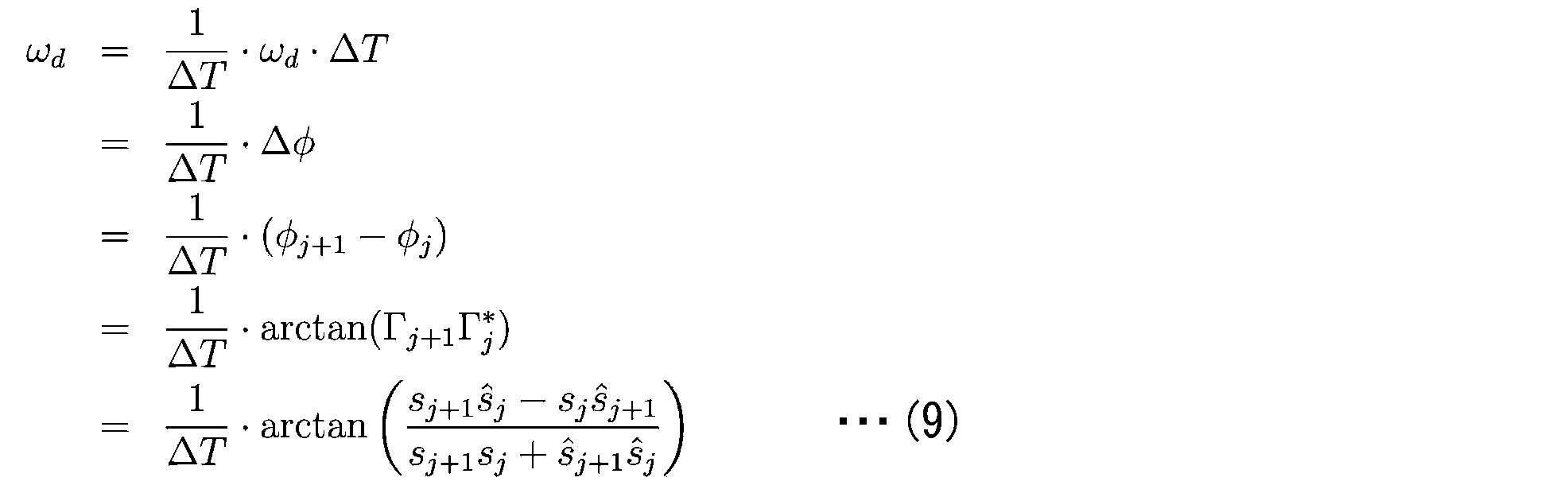
なお,偏角Δφ=ωdΔTであるため、位相の変化量は-π~πの範囲にて検出可能である。また、下記式(10)に従い、n本の干渉信号についてアンサンブル平均処理を施すことにより、ドップラー角周波数シフト量ωdの検出能を向上させることができる。

以上のようにして得られたドップラー角周波数シフト量ωdを上記式(7)に代入することにより、変形速度vを算出できる。この変形速度vに基づいて組織の粘弾性を演算できる。
すなわち、粘弾性体の複素弾性率が下記式(11)のE*で表されることは周知である。複素弾性率E*の実数部分E'は応力とひずみが同位相の成分に相当し、虚数部分E"は応力とひずみが90度位相ずれている成分に相当する。前者のE'は弾性成分に相当し、「貯蔵弾性率」と呼ばれる(以下「貯蔵弾性率E'」という)。後者のE"は応力とひずみ速度が同位相となる粘性成分に相当し、「損失弾性率」と呼ばれる(以下「損失弾性率E"」という)。したがって、貯蔵弾性率E'および損失弾性率E"の分布を、粘弾性の分布として演算できる。
ここで、組織の変形速度vの分布(Z方向の分布)から最小二乗法により各時刻のひずみ量(ひずみ速度)を算出でき、そのひずみ量の振幅(ひずみ振幅ε0)は断層検出できる。また、超音波の音響放射圧の大きさ(応力振幅σ0)は、制御演算部14が超音波デバイス72に対して設定する制御量であるため、把握できる。一方、制御演算部14にて超音波の発振タイミングとOCTの計測タイミングとを把握しているため、応力とひずみの位相差(損失角δ)を算出可能である。したがって、粘弾性パラメータである貯蔵弾性率E'と損失弾性率E"を、それぞれ下記式(11)より算出できる。

このようにして得られた貯蔵弾性率E'と損失弾性率E"の断層分布が、組織の粘弾性の断層分布を実質的に示すことになる。制御演算部14は、その組織の粘弾性を断層可視化する。
一方、上記処理とは異なり、二次元断層画像を予め取得したうえでのポスト処理にはなるが、組織の粘弾性を二次元又は三次元的に断層可視化することができる。この手法は、計測対象の変形前後の2枚のOCT断層画像にデジタル相互相関法を適用することで変形ベクトル分布を算出し、マイクロスケールにて組織のひずみ速度テンソル分布を断層検出する手法である。
変形ベクトル分布を算出する際には、繰り返し相互相関処理を実施する再帰的相互相関法(Recursive Cross-correlation method)を適用する。これは、低解像度において算出された変形ベクトルを参照し、探査領域を限定するとともに階層的に検査領域を縮小して相互相関法を適用する手法である。これにより、高解像度な変形ベクトルを取得することができる。さらに、スペックル・ノイズ低減法として、隣接検査領域の相関値分布との乗算を行う隣接相互相関乗法(Adjacent Cross-correlation Multiplication)を用いる。そして、乗算されることによって高SN化した相関値分布から最大相関値を探索する。
また、マイクロスケールにおける微小変形解析では、変形ベクトルのサブピクセル精度が重要となる。このため、輝度勾配を利用する風上勾配法(Up-stream Gradientmethod)と、伸縮および剪断を考慮した画像変形法(Image Deformation method)の両サブピクセル解析法を併用し、変形ベクトルの高精度検出を実現する。なお、ここでいう「風上勾配法」は、勾配法(オプティカルフロー法)の一種である。
図3は、再帰的相互相関法による処理手順を概略的に示す図である。図4は、サブピクセル解析による処理手順を概略的に示す図である。
(再帰的相互相関法)
図3(A)~(C)は、再帰的相互相関法による処理過程を示している。各図にはOCTにより連続的に撮影される前後の断層画像が示されている。左側には先の断層画像(Image1)が示され、右側には後の断層画像(Image2)が示されている。
図3(A)~(C)は、再帰的相互相関法による処理過程を示している。各図にはOCTにより連続的に撮影される前後の断層画像が示されている。左側には先の断層画像(Image1)が示され、右側には後の断層画像(Image2)が示されている。
相互相関法とは、局所的なスペックル・パターンの類似度を下記式(12)に基づく相関値Rijより評価する方法である。そのため、図3(A)に示すように、連続的に撮影された前後のOCT画像について、先の断層画像(Image1)に類似度の検査対象となる検査領域S1が設定され、後の断層画像(Image2)に類似度の探査範囲となる探査領域S2が設定される。

ここで、空間座標として、光軸方向にZ軸、光軸と垂直方向にX軸を設定している。f(Xi,Zj)とg(Xi,Zj)は、変形前後のOCT画像において設置された中心位置(Xi,Zj)の検査領域S1(Nx×Nzピクセル)のスペックル・パターンを表している。
なお、f-とg-はf(Xi,Zj)とg(Xi,Zj)の検査領域S1内の平均値を表している。
なお、f-とg-はf(Xi,Zj)とg(Xi,Zj)の検査領域S1内の平均値を表している。
探査領域S2(Mx×Mzピクセル)内における相関値分布Ri,j(ΔX,ΔZ)を算出し、図3(B)に示すようにパターンマッチングを行う。実際には、下記式(13)に示すように、最大相関値を与える移動量Ui,jを変形前後の変形ベクトルとして決定する。

本手法では、検査領域S1を縮小しながら相互相関処理を繰り返して空間解像度を高める再帰的相互相関法を採用している。なお、本実施例では解像度を上げる際には空間解像度が倍になるようにしている。図3(C)に示すように、検査領域S1を1/4に分割し、前階層にて算出された変形ベクトルを参照し、探査領域S2を縮小している。ここで探査領域S2も1/4に分割している。再帰的相互相関法を用いることで、高解像度において多発する過誤ベクトルの抑制を可能にしている。このような再帰的相互相関処理を施すことにより、変形ベクトルの解像度を高めることができる。
また、これに加え、下記式(14)により、演算中の座標を中心とする周囲8つの座標を含む合計9つの変形ベクトルの平均偏差σを用いた閾値を設定し、過誤ベクトルの除去を行い再帰処理に伴う誤差伝播を抑制する。

ここで、Umはベクトル量の中央値を表し、閾値となる係数κは任意に設定した。
(隣接相互相関乗法)
本実施例では、スペックルノイズの影響を受けたランダム性の強い相関値分布から正確な最大相関値を決定する方法として、隣接相互相関乗法を導入している。下記式(15)により、隣接相互相関乗法では検査領域S1における相関値分布Ri,j(Δx,Δz)と、その検査領域S1にオーバーラップする隣接検査領域に対するRi+Δi,j(Δx,Δz)とRi,j+Δj(Δx,Δz)の乗算を行い、新たな相関値分布R'i,j(Δx,Δz)を用いて最大相関値を検索する。

本実施例では、スペックルノイズの影響を受けたランダム性の強い相関値分布から正確な最大相関値を決定する方法として、隣接相互相関乗法を導入している。下記式(15)により、隣接相互相関乗法では検査領域S1における相関値分布Ri,j(Δx,Δz)と、その検査領域S1にオーバーラップする隣接検査領域に対するRi+Δi,j(Δx,Δz)とRi,j+Δj(Δx,Δz)の乗算を行い、新たな相関値分布R'i,j(Δx,Δz)を用いて最大相関値を検索する。
これにより、相関値同士の乗算によってランダム性を低減させることが可能になる。上述した検査領域S1の縮小と共に干渉強度分布の情報量も減少するため、スペックル・ノイズを原因とする複数相関ピークの出現が計測精度の悪化を招いていると考えられる。一方、隣接境界同士の移動量には相関があるため、最大相関値座標付近では強い相関値が残存する。この隣接相互相関乗法の導入によって最大相関値ピークが明瞭化され計測精度が向上し、正確な移動座標を抽出することが可能となる。また、この隣接相互相関乗法をOCTの各ステージに導入することで、誤差伝播が抑制され、スペックル・ノイズに対するロバスト性が向上する。それにより、高空間解像度においても高精度な変形ベクトルとひずみ分布の算出が可能となる。
(風上勾配法)
図4(A)~(C)は、サブピクセル解析による処理過程を示している。各図にはOCTにより連続的に撮影される前後の断層画像が示されている。左側には先の断層画像(Image1)が示され、右側には後の断層画像(Image2)が示されている。
図4(A)~(C)は、サブピクセル解析による処理過程を示している。各図にはOCTにより連続的に撮影される前後の断層画像が示されている。左側には先の断層画像(Image1)が示され、右側には後の断層画像(Image2)が示されている。
本実施例では、サブピクセル解析のために風上勾配法と画像変形法を採用する。最終的な移動量の算出は後述の画像変形法によるが、計算の収束性の問題から、画像変形法より先に風上勾配法を適用する。検査領域サイズが小さく高空間解像度の条件において、サブピクセル移動量を高精度検出する画像変形法及び風上勾配法を適用している。画像変形法におけるサブピクセル移動量の検出が困難な場合において、風上勾配法によりサブピクセル移動量を算出する。
サブピクセル解析では、注目点における変形前後の輝度差が各成分の輝度勾配と移動量によって表される。このため、検査領域S1内の輝度勾配データより最小二乗法を用いてサブピクセル移動量を決定することができる。本実施例では、輝度勾配を求める際に、サブピクセル変形前の風上側の輝度勾配を与える風上差分法を採用している。
サブピクセル解析は計測誤差からだけではなく、組織の散乱効果や偏光特性に複雑に関係したスペックル・ノイズに強く依存している。さらに、ひずみテンソル分布の算出には移動量の空間微係数が必要となるため、サブピクセルエラーが微係数算出の数値不安定を増大させ、ひずみテンソル分布の不安定化を招いてしまう。サブピクセル解析は様々な手法が存在するが、本実施例では検査領域サイズが小さく高空間解像度の条件においても、サブピクセル移動量を高精度検出する勾配法を採用している。
風上勾配法は、検査領域S1内の注目点の移動を、図4(A)に示すピクセル精度に留まらず、図4(B)に示すサブピクセル精度にて算出するものである。なお、図中の各格子は1ピクセルを表している。実際には図示の断層画像と比較して相当小さいが、説明の便宜上、大きく表記している。この風上勾配法は、微小変形前後における輝度分布の変化を輝度勾配と移動量によって定式化する手法であり、fを輝度とすると、微小変形f(x+Δx,z+Δz)をテイラー展開する下記式(16)として表される。

上記式(16)は、注目点の変形前後の輝度差が変形前の輝度勾配と移動量によって表されることを示している。なお、移動量(Δx,Δz)については上記式(16)のみでは決定できないため、検査領域S1内で移動量が一定と考え、最小二乗法を適用して算出している。
上記式(16)を用いて移動量を算出する際には、右辺の各注目点における移動前後の輝度差は一意にしか求まらない。そのため輝度勾配をどれだけ正確に算出するかが移動量の精度に直結する。輝度勾配の差分化では、一次精度風上差分を用いている。差分化において高次差分を適用すると、多くのデータが必要になり、ノイズが含まれていた際に影響を大きく受けてしまうためである。また、検査領域S1内の各点を基準とした高次差分では、検査領域S1外のデータを多く使用することとなり、検査領域S1そのものの移動量ではなくなってしまうという問題点も存在するからである。
輝度勾配を求める際に変形前の風上側の輝度勾配が移動することによって注目点の輝度差が生まれると考えることができるので、変形前は風上側の差分を適用する。ここでいう風上は、実際の移動方向ではなく、ピクセル移動量に対するサブピクセル移動量の向きのことであり、最大相関値ピークに放物線近似を施すことによって風上側を決定する。逆に、変形後の風下側の輝度勾配が逆に移動することによって注目点の輝度差が生じると考えることができるため、変形後は風下側の差分を適用する。
変形前の風上差分と変形後の風下差分を用いて2通りの解を求め、それらの平均をとった。さらに、実際には移動量が軸方向に沿わない場合には、変形前や変形後の輝度勾配が注目点と同一軸上に無く、ずれた位置の勾配を求める必要がある。つまり、X方向の勾配を求めたい場合には、Z方向の移動も考慮して勾配を求めなければならない。そのため、輝度の内挿による輝度勾配の推定をすることで、精度向上を図っている。基本的には変形前(もしくは変形後)の位置を予測し、その位置での勾配を内挿により求める。
変形前(後)の注目点の位置は放物線近似を施した際のサブピクセル移動量により求める。その注目点位置が囲まれる8つの座標を用い、それらの比によって輝度勾配を算出する。具体的には、下記式(17)を用いる。そのようにして算出された輝度勾配と、輝度変化を用いて最小二乗法を適用し移動量を決定した。

(画像変形法)
上述した風上勾配法までは検査領域S1の形状は変更せず、正方形を保ったまま変形ベクトルの算出を行っている。しかし、現実には計測対象の変形に合わせて検査領域S1も変形していると考えられるため、検査領域S1の微小変形を考慮したアルゴリズムを導入し、変形ベクトル算出を高精度にて算出する必要がある。このため、本実施例ではサブピクセル精度での変形ベクトルの算出に画像変形法を導入している。すなわち、組織変形前の検査領域S1と組織変形後の伸縮及びせん断変形を考慮した検査領域S1とで相互相関を実施し、相関値ベースの反復計算によってサブピクセル変形量を決定している。なお、検査領域S1の伸縮及びせん断変形は線形で近似している。
上述した風上勾配法までは検査領域S1の形状は変更せず、正方形を保ったまま変形ベクトルの算出を行っている。しかし、現実には計測対象の変形に合わせて検査領域S1も変形していると考えられるため、検査領域S1の微小変形を考慮したアルゴリズムを導入し、変形ベクトル算出を高精度にて算出する必要がある。このため、本実施例ではサブピクセル精度での変形ベクトルの算出に画像変形法を導入している。すなわち、組織変形前の検査領域S1と組織変形後の伸縮及びせん断変形を考慮した検査領域S1とで相互相関を実施し、相関値ベースの反復計算によってサブピクセル変形量を決定している。なお、検査領域S1の伸縮及びせん断変形は線形で近似している。
画像変形法は一般的に、材料の表面ひずみ計測法に用いられ、ランダムパターンを塗布した材料表面を高空間分解能なカメラで撮影した画像に対して適用される。一方、OCT断層像はスペックルノイズを多く含むだけでなく、特に生体組織では組織内の基質や水分の流動も伴い屈折率が変化するため、スペックルパターンに対する変形が大きい。このため、複雑組織にて局所的な変形が発生し、検査領域S1に膨張、収縮、剪断等の変形が伴う場合には解の収束解が著しく低下する。本手法における検査領域S1の縮小は、局所的な組織力学特性を検出するために必要不可欠である。そこで画像変形法では、風上勾配法で得られた変形量を収束計算の初期値として採用し、さらに、輝度分布の双三次関数補間によって検査領域S1を縮小した際でも低ロバスト性を実現している。なお、変形例においては、双三次関数補間以外の補間関数を用いてもよい。
より詳細には、以下の手順にて演算を実行する。まず、組織変形前のOCT断層像の輝度分布に双三次関数補間法を適用し、輝度分布の連続化を実施する。双三次関数補間法とは、sinc関数を区分的に三次関数近似した畳み込み関数を用い、輝度情報の空間連続性を再現する手法である。本来は連続的な輝度分布を画像計測する際には光学系に依存した点広がり関数が畳み込まれるため、sinc関数を用いた逆畳み込みを行うことにより、本来の連続的な輝度分布が復元される。離散的な一軸信号f(x)の補間をする場合、畳み込み関数h(x)は下記式(18)にて表される。

なお、OCT計測条件の違いによって輝度補間関数h(x)の形状も変更する必要がある。そこで輝度補間関数h(x)のx=1での微係数aを可変とし、aの値を変更することで輝度補間関数h(x)の形状を変更可能なアルゴリズムとした。本実施例では、擬似OCT断層像を用いた数値実験による検証結果を元にし、aの値を決定した。以上のように画像補間をすることで、伸縮及びせん断変形を考慮した検査領域S1の各点にて、OCT輝度値を求めることが可能となる。
伸縮及びせん断変形を考慮して算出した検査領域S1は、図4(C)に示すように、移動とともに変形を伴う。組織変形前のOCT断層像におけるある検査領域S1内の整数ピクセル位置での座標(x,z)が組織変形後に座標(x*,z*)に移動すると考えると、x*,z*の値は下記式(19)にて表される。

ここで、Δx,Δzはそれぞれ検査領域S1中心から座標x,zまでの距離、u,vはそれぞれx,z方向への変形量、∂u/∂x,∂v/∂zはそれぞれx,z方向における検査領域S1の垂直方向への変形量、∂u/∂z,∂v/∂xはそれぞれx,z方向における検査領域S1のせん断方向への変形量である。数値解法にはNewton-Raphson法を用い、6変数(u,v,∂u/∂x,∂u/∂z,∂v/∂x,∂v/∂z)での相関値微係数が0となるように、すなわち最大相関値を得るように反復計算を行う。なお、反復計算の収束性を高めるため、x,z方向の移動量初期値には風上勾配法で得られたサブピクセル移動量を用いる。相関値Rに対するヘッセ行列をH、相関値対するヤコビベクトルを▽Rとすると、1回の反復で得られる更新量ΔPiは下記式(20)にて表される。

収束の判定には、反復計算で随時得られる漸近解が収束解の近傍で十分小さくなることを用いる。しかし、スペックルパターンの変化が激しい領域においては、線形変形では追従できないために正しい収束解が得られない場合がある。その場合、本実施例では風上勾配法によって求めたサブピクセル移動量を採用する。このようにして得られるサブピクセル精度の変形ベクトルを時間微分することにより、変形速度ベクトル分布を算出できる。
(時空間移動最小二乗法)
ひずみ速度テンソルの算出には移動最小二乗法(Moving Least Square Method:以下「MLSM」という)を用いる。MLSMは、移動量分布を平滑化すると共に、微係数の安定算出を可能とする手法である。MLSMにおいて用いる二乗誤差式は下記式(21)にて表される。

ひずみ速度テンソルの算出には移動最小二乗法(Moving Least Square Method:以下「MLSM」という)を用いる。MLSMは、移動量分布を平滑化すると共に、微係数の安定算出を可能とする手法である。MLSMにおいて用いる二乗誤差式は下記式(21)にて表される。
上記式(21)において、S(x,z,t)を最小とするa~kのパラメータを求める。すなわち、近似関数として水平方向x,奥行き方向z,時間方向tの3変数2次多項式として下記式(22)を採用する。そして、最小二乗近似に基づき、下記式(23)から最適な微係数を算出して平滑化する。

この微係数を用いることにより、下記式(24)に示すひずみ速度テンソルを算出することができる。fx,fzは各軸のひずみ増分を示し、その時間変化量からひずみ速度を算出している。

上記式(24)にて算出されたひずみ速度を時間積分することにより、ひずみ量を算出でき、そのひずみ量の振幅(ひずみ振幅ε0)は断層検出できる。また、上記式(11)に関連して説明したように、超音波の音響放射圧の大きさ(応力振幅σ0)は、制御演算部14や駆動回路74にて変調振幅として与えることができるため既知であり、応力とひずみの位相差(損失角δ)も算出可能である。よって、粘弾性パラメータである貯蔵弾性率E'と損失弾性率E"を算出できる。このようにして得られた貯蔵弾性率E'と損失弾性率E"の断層分布が、組織の粘弾性の断層分布を実質的に示すことになる。制御演算部14は、その組織の粘弾性を断層可視化する。なお、ひずみ速度のままでも定式化は可能である。つまり、粘弾性パラメータとの対応をとることができる。
次に、制御演算部14が実行する具体的処理の流れについて説明する。
図5は、制御演算部14により実行される粘弾性断層可視化処理の流れを示すフローチャートである。本処理は、所定の演算周期で繰り返し実行される。制御演算部14は、光源2、光学機構8,10および負荷装置13を駆動制御する。それにより、適正に振幅変調された音響放射圧負荷信号を組織に対して入力するとともに(S10)、OCTによる光干渉信号を取得する(S11)。
図5は、制御演算部14により実行される粘弾性断層可視化処理の流れを示すフローチャートである。本処理は、所定の演算周期で繰り返し実行される。制御演算部14は、光源2、光学機構8,10および負荷装置13を駆動制御する。それにより、適正に振幅変調された音響放射圧負荷信号を組織に対して入力するとともに(S10)、OCTによる光干渉信号を取得する(S11)。
制御演算部14は、周波数空間での演算のためにその光干渉信号にフーリエ変換を施して周波数解析する(S12)。続いて、光学機構10での変調周波数に対応づけるようにバンドパスフィルタリング処理を実行して信号SN比を向上させた後(S14)、ヒルベルト変換を実行する(S16)。このヒルベルト変換によって得られた解析信号を用いて、自己相関型リアルタイム粘弾性演算処理を実行する(S18)。また、これと並行して粘弾性断層分布演算処理を実行する(S20)。リアルタイム粘弾性演算処理は、OCT断層画像を取得する過程において、対象Sの組織における一軸方向(Z方向)の粘弾性をほぼリアルタイムに演算し、可視化する処理である。粘弾性断層分布演算処理は、OCT断層画像(二次元画像)を複数取得し、それらに基づいてポスト処理的に組織の粘弾性を断層可視化する処理である。
図6は、図5におけるS18のリアルタイム粘弾性演算処理を詳細に示すフローチャートである。制御演算部14は、S16で取得した解析信号を用いて隣接自己相関処理を施して任意座標における位相差を求め(S30)、ドップラー周波数(ドップラー角周波数シフト量)を得る(S32)。続いて、空間平滑化や空間平均化処理により、組織における変形速度の断層分布を算出する(S34)。この変形速度分布に基づき、最小二乗法を用いてひずみ分布(ひずみ速度分布)を算出し(S36)、上記式(11)に基づいて貯蔵弾性率E'および損失弾性率E"のZ方向分布を算出し(S38)、一軸方向粘弾性を断層可視化する(S40)。
図7は、図5におけるS20の粘弾性断層分布演算処理を詳細に示すフローチャートである。制御演算部14は、解析信号の包絡線(振幅)に基づき、干渉光強度を算出する(S50)。そして、OCT断層画像が所定数取得されると(S52のY)、連続撮影された時刻の異なる前後2枚の断層画像I(x,z,t)とI(x,z,t+Δt)を読み込む(S54)。続いて、再帰的相互相関法による処理を実行する。ここではまず、最小解像度(最大サイズの検査領域)での相互相関処理を実行し、相関係数分布を求める(S56)。続いて、隣接相互相関乗法により、隣接する相関係数分布の積を演算する(S58)。このとき、標準偏差フィルタ等の空間フィルタにより過誤ベクトルの除去をし(S60)、最小二乗法等により除去ベクトルの内挿補間を実行する(S62)。続いて、検査領域を小さくすることによって解像度を上げて相互相関処理を継続する(S64)。すなわち、低解像度での参照ベクトルを基に相互相関処理を実行する。このときの解像度が予め定める最高解像度でなければ(S66のN)、S58に戻る。
そして、S58~S66の処理を繰り返し、最高解像度での相互相関処理が完了すると(S66のY)、サブピクセル解析を実行する。すなわち、最高解像度(最小サイズの検査領域)での変形ベクトルの分布に基づき、風上勾配法によるサブピクセル移動量を演算する(S68)。そして、このとき算出されたサブピクセル移動量に基づき、画像変形法によるサブピクセル変形量を演算する(S70)。続いて、最大相互相関値によるフィルタ処理により過誤ベクトルの除去をし(S72)、最小二乗法等により除去ベクトルの内挿補間を実行する(S74)。そして、このようにして得られた変形ベクトルの時間微分を行い、その断層画像について変形速度ベクトルの断層分布U(x,z,t),W(x,z,t)を算出する(S76)。ここで、U(x,z,t)は変形速度ベクトル分布のz方向成分であり、W(x,z,t)は変形速度ベクトル分布のx方向成分である。以上の処理を後続の断層画像についても実行する(S78のN)。そして、設定数の断層画像について変形ベクトルの断層分布が求まると(S78のY)、粘弾性演算提示処理を実行する(S80)。OCT断層画像が所定数取得されていない場合(S52のN)、本処理を一旦終了する。
図8は、図7におけるS80の粘弾性演算提示処理を詳細に示すフローチャートである。制御演算部6は、時空間移動最小二乗法により、S76にて算出した変形速度ベクトル分布の平滑化を実行する(S90)。そして、その平滑化された変形速度ベクトルにおいて、音響放射圧による加振周波数ω(振幅変調周波数)に同期する成分のみを抽出する(S92)。そして、変形速度ベクトルに対して空間微分をすることにより、ひずみ速度テンソルを算出する(S94)。
続いて、S94で得られたひずみ速度を時間積分することにより、ひずみ量を算出し、そのひずみ量の振幅(ひずみ振幅ε0)の断層分布を演算する。そして上述のように、超音波の音響放射圧の大きさ(応力振幅σ0)と、応力とひずみの位相差(損失角δ)とを用いて貯蔵弾性率E'および損失弾性率E"の断層分布を演算し(S96)、組織の粘弾性を断層可視化する(S98)。なお、ひずみ速度のままでも定式化は可能である。つまり、粘弾性パラメータとの対応をとることができる。
次に、本実施例の効果を評価するために行った検証実験について説明する。
図9および図10は、生体組織を模した試料についての実験結果を表す図である。図9は硬質ゲル試料を用いたときの結果を示し、図10は軟質ゲル試料を用いたときの結果を示す。各図において(A)はOCT断層像を示し、(B)は変形速度(上記式(7)参照)の断層分布を示す。
図9および図10は、生体組織を模した試料についての実験結果を表す図である。図9は硬質ゲル試料を用いたときの結果を示し、図10は軟質ゲル試料を用いたときの結果を示す。各図において(A)はOCT断層像を示し、(B)は変形速度(上記式(7)参照)の断層分布を示す。
本実験では、光源2として中心波長λc=1317nm、半値全幅Δλ=100nmのSLD広帯域光源を用いた。参照鏡26の振れ角を±1.9deg、走査周波数を4kHzに設定し、試料における奥行き走査範囲(Z方向検出範囲)を900μmとした。サンプリング周波数を10MHzとし、Δx=2.5μm間隔で奥行き1軸干渉信号を取得し、1500×900(μm)の断層像を得た。一方、超音波デバイス72を1MHzの基本波にて駆動し、印可音圧をハイドロフォンにて実験前に実測した。
対象Sとして、ヒト皮膚の光学特性を模擬したゲル試料(15mm×15mm×5mm)を用いた。なお、ゲル試料として、ゲル硬化剤の重量パーセントが0.5%の軟質ゲル試料と、ゲル硬化剤の重量パーセントをその4倍にした硬質ゲル試料の2種類を用意し、剛性依存性について断層可視化評価を行った。
図9および図10に示す実験結果によれば、高剛性の硬質ゲル試料では変形速度が小さく、低剛性の軟質ゲル試料では変形速度が大きいことが分かる。このことは、加振力に対して生体組織の低剛性部分は大きく振動し(振幅大)、高剛性部分は小さく振動する(振幅小)という実態に沿ったものと言える。なお、軟質ゲル試料において変形速度に分布があるのは、音響放射圧に分布があるためと考えられる。
図11および図12は、剛性を層状に変化させた層状試料についての実験結果を表す図である。図11は音響放射圧を付与しない状態での実験結果を示し、図12は音響放射圧を付与した状態での実験結果を示す。各図において(A)はOCT断層像を示し、(B)は変形速度の断層分布を示す。層状試料として、表面から200μm程度までを軟質ゲル層、それより下1000μm程度までを硬質ゲル層としたものを用いた。
図11の実験結果によれば、音響放射圧が無負荷の状態では、試料の両層間で違いが見られないことが確認できる。一方、図12の実験結果によれば、軟質ゲル層と硬質ゲル層とで変形速度が異なる(軟質ゲル層のほうが変形速度(振幅)が大きい)ことが分かる。このことは、逆に変形速度の断層可視化によって測定対象における剛性の断層分布(弾性の分布,すなわち上記式(11)におけるE'の断層分布)を評価できることを意味する。
図13は、粘性評価に関する実験結果を表す図である。(A)はOCT断層像を示し、(B)は変形速度の断層分布を示す。(C)は、(B)において奥行方向(Z方向)に変形速度の位相遅れがあることを二点鎖線にて示す。
本実験では、図12に示したものと同様の試料を用いた。OCTにおいてX方向走査を行いつつ、超音波による音響放射圧の振幅を周期的に変化させ、得られる変形速度を断層可視化した。ここでは、その振幅変調周波数を2.4Hzとした。
本実験では、図12に示したものと同様の試料を用いた。OCTにおいてX方向走査を行いつつ、超音波による音響放射圧の振幅を周期的に変化させ、得られる変形速度を断層可視化した。ここでは、その振幅変調周波数を2.4Hzとした。
この実験結果により、奥行き方向に向けて変形速度の位相が遅れる(上層と下層との間で位相がずれる)ことが分かった(二点鎖線の位置が同位相)。これは、音響放射圧により試料に負荷される応力と、それにより発生する変形(ひずみ)との間に位相差(損失角δ)があることを示し、試料に粘性があることを示している。すなわち、以上の実験結果から、粘性の断層分布(粘性係数の分布、すなわち上記式(11)におけるE"の断層分布)を評価できることを意味する。上記実施例によって生体組織の粘弾性の断層検出が可能であることが示唆された。
以上説明したように、本実施例によれば、音響放射圧による非接触の荷重負荷と、OCTによる非接触・非侵襲の断層計測により、対象Sの組織の粘弾性をマイクロ断層可視化する。このため、対象Sが厳格な品質保証を要するものであったとしても、その汚染を防止でき、高精度に力学特性評価を行うことができる。このことが、再生組織のバイオメカニクスの解明にも寄与すると考えられる。
以上、本発明の好適な実施例について説明したが、本発明はその特定の実施例に限定されるものではなく、本発明の技術思想の範囲内で種々の変形が可能であることはいうまでもない。
図14は、変形例に係る荷重負荷方法を表す図である。(A)は第1変形例を示し、(B)は第2変形例を示し、(C)は第3変形例を示す。
第1変形例では、光学機構8と超音波デバイス172とが対象Sに対して同じ側に配置されつつ、OCTによる光軸が焦点Fを通るように設定される。この構成では、振動子アレイ190がドーナツ状に形成され、その中央に孔192が形成される。OCTの光は、この孔192を通って対象Sに照射される。このような構成によれば、負荷装置の支持台に上記実施例のような貫通孔を設ける必要がない。
第1変形例では、光学機構8と超音波デバイス172とが対象Sに対して同じ側に配置されつつ、OCTによる光軸が焦点Fを通るように設定される。この構成では、振動子アレイ190がドーナツ状に形成され、その中央に孔192が形成される。OCTの光は、この孔192を通って対象Sに照射される。このような構成によれば、負荷装置の支持台に上記実施例のような貫通孔を設ける必要がない。
第2変形例では、光学機構8と超音波デバイス72とが対象Sに対して反対側に配置され、OCTによる断層計測の過程で光軸が焦点Fを通らない場合が存在する。例えば、超音波デバイス72の焦点Fを固定し、OCTのX方向走査を行う場合が該当する。本変形例では、焦点FからX方向に所定距離ずれた位置の組織の変形が検出される。一方、第3変形例では、光学機構8と超音波デバイス72とが対象Sに対して同じ側に配置されつつ、OCTによる断層計測の過程で光軸が焦点Fを通らないように設定される。
上記実施例や第1変形例のように、OCTによる光軸が焦点Fを通るように設定すると、OCTによる検出箇所について、音響放射圧の振幅および位相が把握し易いため、演算処理が容易となり、その精度も高くし易い。ただし、機構やデバイスの設置スペースや作動スペースを考慮すると、第2,第3変形例のほうがシステムを構築し易いといったメリットがある。
なお、第2,第3変形例の構成を用いることにより、音響放射圧による組織の変形ではなく、せん断波の伝播速度を検出してもよい。そして、その伝播速度に基づいて組織の粘弾性を判断してもよい。すなわち、音響放射圧による非接触エラストグラフィーを利用し、組織の粘弾性をOCTにより検出してもよい。
上記実施例および変形例では、支持台70を固定し、OCTの光軸および超音波の焦点を移動させる例を示した。変形例においては、支持台70をX方向やY方向に移動制御し、対象Sにおける超音波の焦点やOCTの検出位置を変化させてもよい。
上記実施例では、測定対象を再生組織(培養細胞)とする例を示した。変形例においては、上記装置を生体の再生治療に適用し、組織の生着性をモニタリングしてもよい。上記装置は、軟骨診断や皮膚診断等の医療分野だけでなく、美容整形分野やコズメティック産業分野など、様々な用途および分野に応用できる。
上記実施例では、非接触負荷装置として超音波デバイスを採用し、音響放射圧により組織変形を誘発する例を示した。変形例においては、電気伝導性や磁性を有する粒子(分子標的薬など)を生体組織に取り込ませ、電磁界を照射することにより組織変形を誘発してもよい。
上記実施例では、貯蔵弾性率E'および損失弾性率E"から粘弾性評価を行う例を示したが、これら貯蔵弾性率E'および損失弾性率E"から粘弾性物理量を表現する値を新たに定義し、それに基づいて粘弾性評価を行ってもよい。
上記実施例では、OCTによる断層画像を二次元で取得する例を示したが、三次元で取得してもよい。すなわち、奥行方向(Z方向)とX方向のみならず、Y方向に走査し、組織の粘弾性を断層可視化してもよい。
なお、本発明は上記実施例や変形例に限定されるものではなく、要旨を逸脱しない範囲で構成要素を変形して具体化することができる。上記実施例や変形例に開示されている複数の構成要素を適宜組み合わせることにより種々の発明を形成してもよい。また、上記実施例や変形例に示される全構成要素からいくつかの構成要素を削除してもよい。
Claims (7)
- 光コヒーレンストモグラフィーを用いる光学系を含み、測定対象における組織の粘弾性を断層可視化する粘弾性可視化装置であって、
前記組織に対して変形エネルギーを付与するための負荷装置と、
前記測定対象を経由するオブジェクトアームに設けられ、光源からの光を前記測定対象に導いて走査させる第1光学機構と、
前記測定対象を経由しないリファレンスアームに設けられ、前記光源からの光を参照鏡に導いて反射させる第2光学機構と、
前記測定対象にて反射した物体光と前記参照鏡にて反射した参照光とが重畳された干渉光を検出する光検出装置と、
前記負荷装置および各光学機構の駆動を制御し、それらの駆動に基づいて前記光検出装置から入力された光干渉信号を処理することにより、前記組織の粘弾性の断層分布を演算する制御演算部と、
前記組織の粘弾性を断層可視化する態様で表示する表示装置と、
を備え、
前記負荷装置が、前記測定対象の内部に設定された焦点に向けて超音波を出力することにより、前記組織に対して音響放射圧を負荷する非接触負荷装置であり、
前記制御演算部は、前記光検出装置から入力された光干渉信号に対して周波数解析を実行し、ドップラー周波数を用いて前記組織の変形速度を算出し、その変形速度に基づいて得られるひずみ情報と、前記負荷装置による音響放射圧情報とに基づいて前記組織の粘弾性を演算することを特徴とする粘弾性可視化装置。 - 前記測定対象に向けて照射される光の軸が、前記測定対象における前記音響放射圧の焦点を通るように設定されることを特徴とする請求項1に記載の粘弾性可視化装置。
- 前記制御演算部は、前記組織の変形によって生じる所定の力学特徴量、又は前記組織の変形に伴う所定の力学特徴量の変化を、測定対象の断層位置に対応づけて演算し、その演算結果に基づいて前記組織の粘弾性の断層分布を演算することを特徴とする請求項1または2に記載の粘弾性可視化装置。
- 前記光学機構は、前記測定対象の表面側から光を照射し、
前記負荷装置は、前記測定対象の裏面側から超音波を出力することを特徴とする請求項1~3のいずれかに記載の粘弾性可視化装置。 - 前記測定対象として再生組織を収容するための透光性および音波透過性を有する容器を支持する支持台を備え、
前記支持台は、前記容器の裏面側を露出させるための孔を有することを特徴とする請求項4に記載の粘弾性可視化装置。 - 前記制御演算部は、前記音響放射圧による加振力の位相と、前記ひずみの位相との位相差に基づき、前記組織の粘弾性を演算することを特徴とする請求項1~5のいずれかに記載の粘弾性可視化装置。
- 測定対象の組織の粘弾性を断層可視化する粘弾性可視化方法であって、
前記組織に対して超音波の音響放射圧にて荷重を負荷する負荷工程と、
光コヒーレンストモグラフィーを用いることにより、前記荷重の負荷により変形する前記組織からの後方散乱光に基づく光干渉信号を取得する干渉信号取得工程と、
前記光干渉信号を処理し、前記組織の変形に伴う所定の力学特徴量の変化に基づいて前記組織の粘弾性の断層分布を演算する演算工程と、
前記組織の粘弾性を断層可視化する表示工程と、
を備え、
前記演算工程は、前記光干渉信号に対して周波数解析を実行し、ドップラー周波数を用いて前記組織の変形速度を算出し、その変形速度に基づいて得られるひずみ情報と、前記音響放射圧の情報とに基づいて前記組織の粘弾性を演算することを特徴とする粘弾性可視化方法。
Priority Applications (2)
| Application Number | Priority Date | Filing Date | Title |
|---|---|---|---|
| JP2019518761A JP7154542B2 (ja) | 2017-05-15 | 2018-05-14 | 組織の粘弾性を断層可視化する装置および方法 |
| US16/685,094 US20200077897A1 (en) | 2017-05-15 | 2019-11-15 | Device and method for tomographically visualizing viscoelasticity of tissue |
Applications Claiming Priority (2)
| Application Number | Priority Date | Filing Date | Title |
|---|---|---|---|
| JP2017-096134 | 2017-05-15 | ||
| JP2017096134 | 2017-05-15 |
Related Child Applications (1)
| Application Number | Title | Priority Date | Filing Date |
|---|---|---|---|
| US16/685,094 Continuation US20200077897A1 (en) | 2017-05-15 | 2019-11-15 | Device and method for tomographically visualizing viscoelasticity of tissue |
Publications (1)
| Publication Number | Publication Date |
|---|---|
| WO2018212115A1 true WO2018212115A1 (ja) | 2018-11-22 |
Family
ID=64273726
Family Applications (1)
| Application Number | Title | Priority Date | Filing Date |
|---|---|---|---|
| PCT/JP2018/018455 WO2018212115A1 (ja) | 2017-05-15 | 2018-05-14 | 組織の粘弾性を断層可視化する装置および方法 |
Country Status (3)
| Country | Link |
|---|---|
| US (1) | US20200077897A1 (ja) |
| JP (1) | JP7154542B2 (ja) |
| WO (1) | WO2018212115A1 (ja) |
Families Citing this family (4)
| Publication number | Priority date | Publication date | Assignee | Title |
|---|---|---|---|---|
| US10955323B2 (en) * | 2016-07-21 | 2021-03-23 | National University Corporation NARA Institute of Science and Technology | Method and device for measuring viscoelasticity |
| JP6979510B2 (ja) * | 2018-02-22 | 2021-12-15 | 富士フイルム株式会社 | 内視鏡システム及びその作動方法 |
| CN110864640A (zh) * | 2018-08-28 | 2020-03-06 | 合肥京东方显示技术有限公司 | 光学系统及利用感光相机测量物体应变的方法 |
| WO2023075694A2 (en) * | 2021-10-28 | 2023-05-04 | Agency For Science, Technology And Research | A system and method of non-contact measurement of one or more mechanical properties of a material |
Citations (6)
| Publication number | Priority date | Publication date | Assignee | Title |
|---|---|---|---|---|
| JP2008510585A (ja) * | 2004-08-24 | 2008-04-10 | ザ ジェネラル ホスピタル コーポレイション | 試料の機械的歪み及び弾性的性質を測定するプロセス、システム及びソフトウェア |
| JP2008170363A (ja) * | 2007-01-15 | 2008-07-24 | Olympus Medical Systems Corp | 被検体情報分析装置、内視鏡装置及び被検体情報分析方法 |
| JP2009507208A (ja) * | 2005-05-27 | 2009-02-19 | ボード オブ リージェンツ, ザ ユニバーシティ オブ テキサス システム | 細胞および組成物の光学コヒーレンス断層撮影法による検出 |
| US20100191110A1 (en) * | 2008-12-01 | 2010-07-29 | Insana Michael F | Techniques to evaluate mechanical properties of a biologic material |
| US20150148654A1 (en) * | 2012-06-29 | 2015-05-28 | The General Hospital Corporation | System, method and computer-accessible medium for providing and/or utilizing optical coherence tomographic vibrography |
| WO2016031697A1 (ja) * | 2014-08-26 | 2016-03-03 | 公立大学法人大阪市立大学 | 軟骨診断装置および診断用プローブ |
Family Cites Families (4)
| Publication number | Priority date | Publication date | Assignee | Title |
|---|---|---|---|---|
| WO2002043564A2 (en) * | 2000-11-28 | 2002-06-06 | Allez Physionix Limited | Systems and methods for making non-invasive physiological assessments |
| JP4646716B2 (ja) * | 2005-02-03 | 2011-03-09 | 三洋電機株式会社 | 微生物検出装置及び微生物検出用カセット |
| DE102009043524A1 (de) * | 2009-09-30 | 2011-03-31 | Siemens Healthcare Diagnostics Products Gmbh | Vorrichtung für die photometrische Untersuchung von Proben |
| WO2011153268A2 (en) * | 2010-06-01 | 2011-12-08 | The Trustees Of Columbia University In The City Of New York | Devices, methods, and systems for measuring elastic properties of biological tissues |
-
2018
- 2018-05-14 WO PCT/JP2018/018455 patent/WO2018212115A1/ja active Application Filing
- 2018-05-14 JP JP2019518761A patent/JP7154542B2/ja active Active
-
2019
- 2019-11-15 US US16/685,094 patent/US20200077897A1/en active Pending
Patent Citations (6)
| Publication number | Priority date | Publication date | Assignee | Title |
|---|---|---|---|---|
| JP2008510585A (ja) * | 2004-08-24 | 2008-04-10 | ザ ジェネラル ホスピタル コーポレイション | 試料の機械的歪み及び弾性的性質を測定するプロセス、システム及びソフトウェア |
| JP2009507208A (ja) * | 2005-05-27 | 2009-02-19 | ボード オブ リージェンツ, ザ ユニバーシティ オブ テキサス システム | 細胞および組成物の光学コヒーレンス断層撮影法による検出 |
| JP2008170363A (ja) * | 2007-01-15 | 2008-07-24 | Olympus Medical Systems Corp | 被検体情報分析装置、内視鏡装置及び被検体情報分析方法 |
| US20100191110A1 (en) * | 2008-12-01 | 2010-07-29 | Insana Michael F | Techniques to evaluate mechanical properties of a biologic material |
| US20150148654A1 (en) * | 2012-06-29 | 2015-05-28 | The General Hospital Corporation | System, method and computer-accessible medium for providing and/or utilizing optical coherence tomographic vibrography |
| WO2016031697A1 (ja) * | 2014-08-26 | 2016-03-03 | 公立大学法人大阪市立大学 | 軟骨診断装置および診断用プローブ |
Non-Patent Citations (2)
| Title |
|---|
| QU, Y. Q. ET AL.: "Acoustic radiation force optical coherence elastography of corneal tissue", IEEE JOURNAL OF SELECTED TOPICS IN QUANTUM ELECTRONICS, vol. 22, no. 3, 25 April 2016 (2016-04-25), pages 1 - 7, XP011607504 * |
| ZHU, J. ET AL.: "Imaging and characterizing shear wave and shear modulus under orthogonal acoustic radiation force excitation using OCT Doppler variance method", OPTICS LETTERS, vol. 40, no. 9, 1 May 2015 (2015-05-01), pages 2099 - 2102, XP055561834 * |
Also Published As
| Publication number | Publication date |
|---|---|
| US20200077897A1 (en) | 2020-03-12 |
| JP7154542B2 (ja) | 2022-10-18 |
| JPWO2018212115A1 (ja) | 2020-03-12 |
Similar Documents
| Publication | Publication Date | Title |
|---|---|---|
| TWI735596B (zh) | 皮膚診斷裝置、皮膚狀態輸出方法、電腦程式產品及記錄媒體 | |
| Song et al. | Tracking mechanical wave propagation within tissue using phase-sensitive optical coherence tomography: motion artifact and its compensation | |
| WO2018212115A1 (ja) | 組織の粘弾性を断層可視化する装置および方法 | |
| Song et al. | Shear modulus imaging by direct visualization of propagating shear waves with phase-sensitive optical coherence tomography | |
| Zvietcovich et al. | Comparative study of shear wave-based elastography techniques in optical coherence tomography | |
| JP5486046B2 (ja) | 変位計測方法及び装置 | |
| JP6707258B2 (ja) | 応力可視化装置および力学物性値可視化装置 | |
| US20150009507A1 (en) | Swept source optical coherence tomography and method for stabilizing phase thereof | |
| KR101704113B1 (ko) | 편광 감응식 광 간섭 단층 촬영의 편광 데이터를 처리하기 위한 방법 및 장치 | |
| JP2010505127A (ja) | 生体環境中での構造および流れの撮像 | |
| US9693728B2 (en) | Systems and methods for measuring mechanical properties of deformable materials | |
| EP2784438B1 (en) | Method for generating two-dimensional images from three-dimensional optical coherence tomography interferogram data | |
| JP2007152074A (ja) | 変位又は歪計測方法及び装置、速度計測方法、弾性率・粘弾性率計測装置、及び、超音波診断装置 | |
| Smith et al. | Optimum scan spacing for three-dimensional ultrasound by speckle statistics | |
| JP6623163B2 (ja) | 軟骨診断装置および診断用プローブ | |
| JP6648891B2 (ja) | 物質含有量を断層可視化する装置および方法 | |
| Beuve et al. | Diffuse shear wave spectroscopy for soft tissue viscoelastic characterization | |
| Claus et al. | Large-field-of-view optical elastography using digital image correlation for biological soft tissue investigation | |
| Claeson et al. | Marker-free tracking of facet capsule motion using polarization-sensitive optical coherence tomography | |
| Buchta et al. | Soft tissue elastography via shearing interferometry | |
| Chen et al. | Quantitative reconstruction of a disturbed ultrasound pressure field in a conventional hydrophone measurement | |
| Almqvist et al. | High resolution light diffraction tomography: nearfield measurements of 10 MHz continuous wave ultrasound | |
| Zvietcovich | Dynamic optical coherence elastography | |
| JP7174993B2 (ja) | マイクロ断層可視化装置および方法 | |
| Zvietcovich et al. | A comparative study of shear wave speed estimation techniques in optical coherence elastography applications |
Legal Events
| Date | Code | Title | Description |
|---|---|---|---|
| 121 | Ep: the epo has been informed by wipo that ep was designated in this application |
Ref document number: 18802534 Country of ref document: EP Kind code of ref document: A1 |
|
| ENP | Entry into the national phase |
Ref document number: 2019518761 Country of ref document: JP Kind code of ref document: A |
|
| NENP | Non-entry into the national phase |
Ref country code: DE |
|
| 122 | Ep: pct application non-entry in european phase |
Ref document number: 18802534 Country of ref document: EP Kind code of ref document: A1 |