US9638831B1 - Computer-implemented system and method for generating a risk-adjusted probabilistic forecast of renewable power production for a fleet - Google Patents
Computer-implemented system and method for generating a risk-adjusted probabilistic forecast of renewable power production for a fleet Download PDFInfo
- Publication number
- US9638831B1 US9638831B1 US14/139,007 US201314139007A US9638831B1 US 9638831 B1 US9638831 B1 US 9638831B1 US 201314139007 A US201314139007 A US 201314139007A US 9638831 B1 US9638831 B1 US 9638831B1
- Authority
- US
- United States
- Prior art keywords
- irradiance
- clearness
- error
- power
- normalized
- Prior art date
- Legal status (The legal status is an assumption and is not a legal conclusion. Google has not performed a legal analysis and makes no representation as to the accuracy of the status listed.)
- Active, expires
Links
- 238000004519 manufacturing process Methods 0.000 title claims abstract description 103
- 238000000034 method Methods 0.000 title description 48
- 230000006870 function Effects 0.000 claims description 63
- 238000010248 power generation Methods 0.000 abstract description 23
- 230000008859 change Effects 0.000 description 55
- 238000013459 approach Methods 0.000 description 29
- 238000004364 calculation method Methods 0.000 description 28
- 238000005259 measurement Methods 0.000 description 26
- 239000011159 matrix material Substances 0.000 description 25
- 238000004088 simulation Methods 0.000 description 21
- 230000000875 corresponding effect Effects 0.000 description 12
- 238000009826 distribution Methods 0.000 description 12
- 230000010354 integration Effects 0.000 description 12
- RZVAJINKPMORJF-UHFFFAOYSA-N Acetaminophen Chemical compound CC(=O)NC1=CC=C(O)C=C1 RZVAJINKPMORJF-UHFFFAOYSA-N 0.000 description 11
- 238000010586 diagram Methods 0.000 description 11
- 238000004458 analytical method Methods 0.000 description 10
- 238000011156 evaluation Methods 0.000 description 10
- 238000006243 chemical reaction Methods 0.000 description 8
- 230000005611 electricity Effects 0.000 description 8
- 230000002123 temporal effect Effects 0.000 description 8
- 230000005855 radiation Effects 0.000 description 7
- 230000009467 reduction Effects 0.000 description 7
- 230000014509 gene expression Effects 0.000 description 6
- 238000012545 processing Methods 0.000 description 6
- 230000003247 decreasing effect Effects 0.000 description 5
- 230000000694 effects Effects 0.000 description 5
- 230000001186 cumulative effect Effects 0.000 description 4
- 238000005315 distribution function Methods 0.000 description 4
- 239000000203 mixture Substances 0.000 description 4
- 238000012544 monitoring process Methods 0.000 description 4
- 238000004891 communication Methods 0.000 description 3
- 230000002596 correlated effect Effects 0.000 description 3
- 238000013480 data collection Methods 0.000 description 3
- 238000009472 formulation Methods 0.000 description 3
- 238000003860 storage Methods 0.000 description 3
- 238000006467 substitution reaction Methods 0.000 description 3
- 238000013519 translation Methods 0.000 description 3
- 230000006399 behavior Effects 0.000 description 2
- 230000005540 biological transmission Effects 0.000 description 2
- 238000005094 computer simulation Methods 0.000 description 2
- 238000009795 derivation Methods 0.000 description 2
- 238000009499 grossing Methods 0.000 description 2
- 238000009434 installation Methods 0.000 description 2
- 238000012806 monitoring device Methods 0.000 description 2
- 230000008569 process Effects 0.000 description 2
- 238000005070 sampling Methods 0.000 description 2
- 239000004065 semiconductor Substances 0.000 description 2
- 229930091051 Arenine Natural products 0.000 description 1
- 239000002028 Biomass Substances 0.000 description 1
- 230000002411 adverse Effects 0.000 description 1
- 230000003466 anti-cipated effect Effects 0.000 description 1
- 238000003491 array Methods 0.000 description 1
- 230000008901 benefit Effects 0.000 description 1
- 239000002551 biofuel Substances 0.000 description 1
- 230000033228 biological regulation Effects 0.000 description 1
- 244000309464 bull Species 0.000 description 1
- 230000001364 causal effect Effects 0.000 description 1
- 239000002800 charge carrier Substances 0.000 description 1
- 238000004590 computer program Methods 0.000 description 1
- 239000000470 constituent Substances 0.000 description 1
- 238000005314 correlation function Methods 0.000 description 1
- 230000007423 decrease Effects 0.000 description 1
- 230000001419 dependent effect Effects 0.000 description 1
- 238000013461 design Methods 0.000 description 1
- 238000011161 development Methods 0.000 description 1
- 239000006185 dispersion Substances 0.000 description 1
- 230000001747 exhibiting effect Effects 0.000 description 1
- ZZUFCTLCJUWOSV-UHFFFAOYSA-N furosemide Chemical compound C1=C(Cl)C(S(=O)(=O)N)=CC(C(O)=O)=C1NCC1=CC=CO1 ZZUFCTLCJUWOSV-UHFFFAOYSA-N 0.000 description 1
- 230000006872 improvement Effects 0.000 description 1
- 238000011835 investigation Methods 0.000 description 1
- 238000012986 modification Methods 0.000 description 1
- 230000004048 modification Effects 0.000 description 1
- 238000005457 optimization Methods 0.000 description 1
- 238000011958 production data acquisition Methods 0.000 description 1
- 238000012887 quadratic function Methods 0.000 description 1
- 238000011160 research Methods 0.000 description 1
- 230000002441 reversible effect Effects 0.000 description 1
- 238000000926 separation method Methods 0.000 description 1
- 238000012163 sequencing technique Methods 0.000 description 1
- 230000000153 supplemental effect Effects 0.000 description 1
- 230000001360 synchronised effect Effects 0.000 description 1
- 238000012360 testing method Methods 0.000 description 1
- 238000010200 validation analysis Methods 0.000 description 1
Images


Classifications
-
- G—PHYSICS
- G06—COMPUTING; CALCULATING OR COUNTING
- G06Q—INFORMATION AND COMMUNICATION TECHNOLOGY [ICT] SPECIALLY ADAPTED FOR ADMINISTRATIVE, COMMERCIAL, FINANCIAL, MANAGERIAL OR SUPERVISORY PURPOSES; SYSTEMS OR METHODS SPECIALLY ADAPTED FOR ADMINISTRATIVE, COMMERCIAL, FINANCIAL, MANAGERIAL OR SUPERVISORY PURPOSES, NOT OTHERWISE PROVIDED FOR
- G06Q50/00—Information and communication technology [ICT] specially adapted for implementation of business processes of specific business sectors, e.g. utilities or tourism
- G06Q50/06—Energy or water supply
-
- G—PHYSICS
- G01—MEASURING; TESTING
- G01W—METEOROLOGY
- G01W1/00—Meteorology
- G01W1/10—Devices for predicting weather conditions
-
- G—PHYSICS
- G06—COMPUTING; CALCULATING OR COUNTING
- G06Q—INFORMATION AND COMMUNICATION TECHNOLOGY [ICT] SPECIALLY ADAPTED FOR ADMINISTRATIVE, COMMERCIAL, FINANCIAL, MANAGERIAL OR SUPERVISORY PURPOSES; SYSTEMS OR METHODS SPECIALLY ADAPTED FOR ADMINISTRATIVE, COMMERCIAL, FINANCIAL, MANAGERIAL OR SUPERVISORY PURPOSES, NOT OTHERWISE PROVIDED FOR
- G06Q10/00—Administration; Management
- G06Q10/06—Resources, workflows, human or project management; Enterprise or organisation planning; Enterprise or organisation modelling
- G06Q10/063—Operations research, analysis or management
- G06Q10/0631—Resource planning, allocation, distributing or scheduling for enterprises or organisations
- G06Q10/06315—Needs-based resource requirements planning or analysis
-
- G—PHYSICS
- G06—COMPUTING; CALCULATING OR COUNTING
- G06Q—INFORMATION AND COMMUNICATION TECHNOLOGY [ICT] SPECIALLY ADAPTED FOR ADMINISTRATIVE, COMMERCIAL, FINANCIAL, MANAGERIAL OR SUPERVISORY PURPOSES; SYSTEMS OR METHODS SPECIALLY ADAPTED FOR ADMINISTRATIVE, COMMERCIAL, FINANCIAL, MANAGERIAL OR SUPERVISORY PURPOSES, NOT OTHERWISE PROVIDED FOR
- G06Q10/00—Administration; Management
- G06Q10/06—Resources, workflows, human or project management; Enterprise or organisation planning; Enterprise or organisation modelling
- G06Q10/063—Operations research, analysis or management
- G06Q10/0635—Risk analysis of enterprise or organisation activities
-
- H—ELECTRICITY
- H02—GENERATION; CONVERSION OR DISTRIBUTION OF ELECTRIC POWER
- H02J—CIRCUIT ARRANGEMENTS OR SYSTEMS FOR SUPPLYING OR DISTRIBUTING ELECTRIC POWER; SYSTEMS FOR STORING ELECTRIC ENERGY
- H02J2203/00—Indexing scheme relating to details of circuit arrangements for AC mains or AC distribution networks
- H02J2203/20—Simulating, e g planning, reliability check, modelling or computer assisted design [CAD]
-
- Y—GENERAL TAGGING OF NEW TECHNOLOGICAL DEVELOPMENTS; GENERAL TAGGING OF CROSS-SECTIONAL TECHNOLOGIES SPANNING OVER SEVERAL SECTIONS OF THE IPC; TECHNICAL SUBJECTS COVERED BY FORMER USPC CROSS-REFERENCE ART COLLECTIONS [XRACs] AND DIGESTS
- Y02—TECHNOLOGIES OR APPLICATIONS FOR MITIGATION OR ADAPTATION AGAINST CLIMATE CHANGE
- Y02E—REDUCTION OF GREENHOUSE GAS [GHG] EMISSIONS, RELATED TO ENERGY GENERATION, TRANSMISSION OR DISTRIBUTION
- Y02E10/00—Energy generation through renewable energy sources
- Y02E10/50—Photovoltaic [PV] energy
- Y02E10/56—Power conversion systems, e.g. maximum power point trackers
-
- Y—GENERAL TAGGING OF NEW TECHNOLOGICAL DEVELOPMENTS; GENERAL TAGGING OF CROSS-SECTIONAL TECHNOLOGIES SPANNING OVER SEVERAL SECTIONS OF THE IPC; TECHNICAL SUBJECTS COVERED BY FORMER USPC CROSS-REFERENCE ART COLLECTIONS [XRACs] AND DIGESTS
- Y04—INFORMATION OR COMMUNICATION TECHNOLOGIES HAVING AN IMPACT ON OTHER TECHNOLOGY AREAS
- Y04S—SYSTEMS INTEGRATING TECHNOLOGIES RELATED TO POWER NETWORK OPERATION, COMMUNICATION OR INFORMATION TECHNOLOGIES FOR IMPROVING THE ELECTRICAL POWER GENERATION, TRANSMISSION, DISTRIBUTION, MANAGEMENT OR USAGE, i.e. SMART GRIDS
- Y04S10/00—Systems supporting electrical power generation, transmission or distribution
- Y04S10/50—Systems or methods supporting the power network operation or management, involving a certain degree of interaction with the load-side end user applications
Definitions
- This application relates in general to renewable energy fleet forecasting and, in particular, to a computer-implemented system and method for generating a risk-adjusted probabilistic forecast of renewable power production for a fleet.
- photovoltaic systems have advanced significantly in recent years due to a continually growing demand for renewable energy resources of all types, including wind, hydro, biomass, geothermal, and biofuel.
- the cost per watt of electricity generated by photovoltaic systems has decreased more dramatically than in earlier systems, especially when combined with government incentives offered to encourage photovoltaic power generation.
- photovoltaic systems are collectively operated as a fleet, although the individual systems in the fleet may be deployed at different physical locations within a geographic region.
- a power grid is an electricity generation, transmission, and distribution infrastructure that delivers electricity from supplies to consumers. Both planners and operators of power grids need to be able to accurately gauge on-going and expected power generation and consumption.
- power generation forecasts for most forms of renewable energy resources are accompanied by a degree of uncertainty that is statistically quantified, for example, through mean and standard deviation.
- the power generation forecasts received by power grid planners and operators alike are only a part of the information necessary to properly operate the power grid.
- many planners and operators prefer to receive just one power generation forecast per source of renewable energy, such as a renewable power production fleet.
- statistical uncertainty is insufficient to aid planners and operators in balancing the costs and risks inherent in the power grid operational decision-making process.
- photovoltaic production forecasting first requires choosing a type of solar resource appropriate to the form of simulation.
- the solar resource data is then combined with each plant's system configuration in a photovoltaic simulation model, which generates a forecast of photovoltaic production.
- Confusion exists about the relationship between irradiance and irradiation, their respective applicability to forecasting, and how to correctly calculate normalized irradiation.
- solar power forecasting requires irradiance, which is an instantaneous measure of solar radiation that can be derived from a single ground-based observation, satellite imagery, numerical weather prediction models, or other sources.
- Solar energy forecasting requires normalized irradiation, which is an interval measure of solar radiation measured or projected over a time period.
- irradiance and normalized irradiation reverse conventional uses of time as measures of proportionality, where rate is merely expressed as W/m 2 (watts per square meter) and non-normalized quantity, that is, irradiation, is expressed as W/m 2 /h (watts per square meter per hour), or, in normalized form, using the same units as rate, W/m 2 . Using the same units for both rate and quantity contributes to confusion. Irradiance and normalized irradiation are only guaranteed to be equivalent if the irradiance is constant over the time interval over which normalized irradiation is solved. This situation rarely occurs since the sun's position in the sky is constantly changing, albeit at a very slow rate.
- Photovoltaic system power output is particularly sensitive to shading due to cloud cover.
- photovoltaic fleets that combine individual plants physically scattered over a geographical area may be subject to different weather conditions due to cloud cover and cloud speed with an effect on aggregate fleet power output.
- Photovoltaic fleets operating under cloudy conditions can exhibit variable and potentially unpredictable performance.
- fleet variability is determined by collecting and feeding direct power measurements from individual photovoltaic systems or indirectly-derived power measurements into a centralized control computer or similar arrangement.
- the practicality of such an approach diminishes as the number of systems, variations in system configurations, and geographic dispersion of the fleet grow.
- one direct approach to obtaining high speed time series power production data from a fleet of existing photovoltaic systems is to install physical meters on every photovoltaic system, record the electrical power output at a desired time interval, such as every 10 seconds, and sum the recorded output across all photovoltaic systems in the fleet at each time interval.
- An equivalent direct approach to obtaining high speed time series power production data is to collect solar irradiance data from a dense network of weather monitoring stations covering all anticipated locations at the desired time interval, use a photovoltaic performance model to simulate the high speed time series output data for each photovoltaic system individually, and then sum the results at each time interval.
- both direct approaches only work when and where meters are pre-installed; thus, high speed time series power production data is unavailable for all other locations, time periods, and photovoltaic system configurations. Both direct approaches also cannot be used to directly forecast future photovoltaic system performance since meters must be physically present at the time and location of interest. Data also must be recorded at the time resolution that corresponds to the desired output time resolution. While low time-resolution results can be calculated from high resolution data, the opposite calculation is not possible.
- satellite irradiance data for specific locations and time periods have been combined with randomly selected high speed data from a limited number of ground-based weather stations, such as described in CAISO 2011. “Summary of Preliminary Results of 33% Renewable Integration Study—2010,” Cal. Pub. Util. Comm. LTPP Docket No. R.10-05-006 (Apr. 29, 2011) and J. Stein, “Simulation of 1-Minute Power Output from Utility-Scale Photovoltaic Generation Systems,” Am. Solar Energy Soc. Annual Conf. Procs., Raleigh, N.C. (May 18, 2011), the disclosures of which are incorporated by reference.
- This approach does not produce time synchronized photovoltaic fleet variability for specific time periods because the locations of the ground-based weather stations differ from the actual locations of the fleet.
- Probabilistic forecasts of the expected power production of renewable power sources are generally provided with a degree of uncertainty.
- the expected power production for a fleet can be projected as a time series of power production estimates over a time period ahead of the current time.
- the uncertainty of each power production estimate can be combined with the costs and risks associated with power generation forecasting errors, and displayed or visually graphed as a single, deterministic result to assist power grid operators (or planners) in deciding whether to rely on the renewable power source.
- One embodiment provides a computer-implemented system and method for generating a risk-adjusted probabilistic forecast of renewable power production for a fleet.
- a set of clearness indexes is built by dividing irradiance observations measured at regular intervals for the location of a renewable power production plant by clear sky irradiance.
- the set of clearness indexes is ordered into a time series successively spaced at input time intervals.
- a clearness correlation coefficient between the location of the renewable power production plant and the location of one other renewable power production plant in the same power production fleet is found as a function of physical distance between the two plants in proportion to overhead cloud speed.
- the set of clearness indexes is weighted by the clearness correlation coefficient.
- the set of weighted clearness indexes is ordered into a time series at the input time intervals.
- Expected power production statistics are estimated from the time series of the clearness indexes and the time series of the weighted clearness indexes.
- Expected power production is forecast as a function of the expected power production statistics and overall power ratings of the two renewable power production plants.
- a time lag correlation coefficient is applied to the expected power production to build a time series at output time intervals. Error associated with the expected power production for at least one of the output time intervals of the time series of the expected power production is determined. Risk associated with the error is identified. The expected power production is adjusted based on the risk.
- FIG. 1 is a flow diagram showing a computer-implemented method for generating a risk-adjusted probabilistic forecast of renewable power production for a fleet in accordance with one embodiment.
- FIG. 2 is a block diagram showing a computer-implemented system for generating a risk-adjusted probabilistic forecast of renewable power production for a fleet in accordance with one embodiment.
- FIG. 3 is a graph depicting, by way of example, ten hours of time series irradiance data collected from a ground-based weather station with 10-second resolution.
- FIG. 4 is a graph depicting, by way of example, the clearness index that corresponds to the irradiance data presented in FIG. 3 .
- FIG. 5 is a graph depicting, by way of example, the change in clearness index that corresponds to the clearness index presented in FIG. 4 .
- FIG. 6 is a graph depicting, by way of example, the irradiance statistics that correspond to the clearness index in FIG. 4 and the change in clearness index in FIG. 5 .
- FIG. 7 is a flow diagram showing a function for determining variance for use with the method of FIG. 1 .
- FIG. 8 is a block diagram showing, by way of example, nine evenly-spaced points within a three-by-three correlation region for evaluation by the function of FIG. 7 .
- FIG. 9 is a block diagram showing, by way of example, 16 evenly-spaced points within a three-by-three correlation region for evaluation by the function of FIG. 7 .
- FIG. 10 is a graph depicting, by way of example, the number of calculations required when determining variance using three different approaches.
- FIG. 11 is a screen shot showing, by way of example, a user interface of the SolarAnywhere service.
- FIGS. 12A-12B are graphs showing, by way of example, a sample day of solar irradiance plotted respectively based on the centered on satellite measurement time and standard top of hour, end of period integration formats.
- FIGS. 13A-13B are graphs respectively showing, by way of example, a sample day of irradiance and clearness indexes.
- FIGS. 14A-14B are graphs respectively showing, by way of example, two-hour periods of the irradiance and clearness indexes of the sample day of FIGS. 12A-12B .
- FIG. 15 is a graph showing, by way of example, normalized irradiation equated to irradiance based on the irradiance plotted in FIG. 14A .
- FIG. 16 is a graph showing, by way of example, normalized irradiation determined through linear interpolation of the irradiance plotted in FIG. 14A .
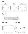
- FIG. 17 is a graph showing, by way of example, three cases of determining normalized irradiation through linear interpolation of the irradiance plotted in FIG. 14A .
- FIG. 18 is a table presenting, by way of example, the normalized irradiation calculated for the three cases of FIG. 17 .
- FIGS. 19A-19B are graphs respectively showing, by way of example, determining clearness indexes through linear interpolation of the irradiance plotted of FIGS. 12A-12B .
- FIG. 20 is a table presenting, by way of example, the weighting factors for calculating normalized irradiation for start at top of hour (or half-hour for Enhanced Resolution data) with end of period integration for the three cases of FIG. 17 .
- FIG. 21 is a table presenting, by way of example, the relative Mean Absolute Error for irradiance and normalized irradiation for the normalized irradiation estimates for the ten locations and resolution scenarios.
- FIG. 22 is a graph showing, by way of example, the relative reduction in relative Mean Absolute Error for the normalized irradiation estimates for the ten locations and resolution scenarios.
- FIG. 23 is a set of graphs showing, by way of example, Standard Resolution data (half-hour, 1-km) in Hanford, Calif., 2012 for the tuned versus un-tuned irradiance and normalized irradiation.
- FIG. 24 is a set of graphs showing, by way of example, Enhanced Resolution data (half-hour, 1-km) in Hanford, Calif., 2012 for the tuned versus un-tuned irradiance and normalized irradiation.
- FIG. 25 is a set of graphs showing, by way of example, Enhanced Resolution data (half-hour, 1-km) in Campbell, Hi., first half of 2012 for the tuned versus un-tuned irradiance and normalized irradiation.
- FIG. 26 is a set of graphs showing, by way of example, Standard Resolution data (half-hour, 1-km) in Penn State, PA, 2012 for the tuned versus un-tuned irradiance and normalized irradiation.
- FIG. 27 is a set of graphs showing, by way of example, Standard Resolution data (half-hour, 1-km) in Boulder, Colo., 2012 for the tuned versus un-tuned irradiance and normalized irradiation.
- FIG. 28 is a graph showing, by way of example, error cost as a function of forecasted renewable power production.
- FIGS. 29A-29B are photographs showing, by way of example, the locations of the Cordelia Junction and Napa high density weather monitoring stations.
- FIGS. 30A-30B are graphs depicting, by way of example, the adjustment factors plotted for time intervals from 10 seconds to 300 seconds.
- FIGS. 31A-31F are graphs depicting, by way of example, the measured and predicted weighted average correlation coefficients for each pair of locations versus distance.
- FIGS. 32A-32F are graphs depicting, by way of example, the same information as depicted in FIGS. 31A-31F versus temporal distance.
- FIGS. 33A-33F are graphs depicting, by way of example, the predicted versus the measured variances of clearness indexes using different reference time intervals.
- FIGS. 34A-34F are graphs depicting, by way of example, the predicted versus the measured variances of change in clearness indexes using different reference time intervals.
- FIGS. 35A-35F are graphs and a diagram depicting, by way of example, application of the methodology described herein to the Napa network.
- FIG. 36 is a graph depicting, by way of example, an actual probability distribution for a given distance between two pairs of locations, as calculated for a 1,000 meter ⁇ 1,000 meter grid in one square meter increments.
- FIG. 37 is a graph depicting, by way of example, a matching of the resulting model to an actual distribution.
- FIG. 38 is a graph depicting, by way of example, results generated by application of Equation (87).
- FIG. 39 is a graph depicting, by way of example, the probability density function when regions are spaced by zero to five regions.
- FIG. 40 is a graph depicting, by way of example, results by application of the model.
- Photovoltaic cells employ semiconductors exhibiting a photovoltaic effect to generate direct current electricity through conversion of solar irradiance. Within each photovoltaic cell, light photons excite electrons in the semiconductors to create a higher state of energy, which acts as a charge carrier for the electrical current. The direct current electricity is converted by power inverters into alternating current electricity, which is then output for use in a power grid or other destination consumer.
- a photovoltaic system uses one or more photovoltaic panels that are linked into an array to convert sunlight into electricity.
- a single photovoltaic plant can include one or more of these photovoltaic arrays.
- a collection of photovoltaic plants can be collectively operated as a photovoltaic fleet that is integrated into a power grid, although the constituent photovoltaic plants within the fleet may actually be deployed at different physical locations spread out over a geographic region.
- FIG. 1 is a flow diagram showing a computer-implemented method 10 for generating a risk-adjusted probabilistic forecast of renewable power production for a fleet in accordance with one embodiment.
- the method 10 can be implemented in software and execution of the software can be performed on a computer system, such as further described infra, as a series of process or method modules or steps.
- a time series of solar irradiance or photovoltaic (“PV”) data is first obtained (step 11 ) for a set of locations representative of the geographic region within which the photovoltaic fleet is located or intended to operate, as further described infra with reference to FIG. 3 .
- Each time series contains solar irradiance observations, which are instantaneous measures associated with a single observation time that are measured or derived, then electronically recorded at a known sampling rate at fixed time intervals, such as at half-hour intervals, over successive observational time periods.
- the solar irradiance observations can include solar irradiance measured by a representative set of ground-based weather stations (step 12 ), existing photovoltaic systems (step 13 ), satellite observations (step 14 ), or some combination thereof.
- Other sources of the solar irradiance data are possible, including numeric weather prediction models.
- the solar irradiance data in the time series is converted over each of the time periods, such as at half-hour intervals, into a set of global horizontal irradiance (GHI) clearness indexes, which are calculated relative to clear sky global horizontal irradiance based on the type of solar irradiance data, such as described in commonly-assigned U.S. patent application, entitled “Computer-Implemented Method for Tuning Photovoltaic Power Generation Plant Forecasting,” Ser. No. 13/677,175, filed Nov. 14, 2012, pending, the disclosure of which is incorporated by reference.
- the set of clearness indexes can be interpreted into irradiance statistics (step 15 ), as further described infra with reference to FIGS. 4-6 .
- the solar irradiance data and, in a further embodiment, the set of clearness indexes can also be interpreted into normalized irradiation (step 18 ), as further described infra with reference to FIGS. 11-27 .
- the calculated irradiance statistics are combined with the photovoltaic fleet configuration to generate the high-speed time series photovoltaic production data.
- Output data that can include a probabilistic forecast of power and energy data for the photovoltaic plant (or other type of renewable energy source, as applicable), including a time series of the power statistics, are generated (step 17 ) as a function of the irradiance statistics, photovoltaic plant configuration (step 16 ), and, if applicable, normalized irradiation.
- the photovoltaic plant configuration includes power generation and location information, including direct current (“DC”) plant and photovoltaic panel ratings; number of power inverters; latitude, longitude and elevation; sampling and recording rates; sensor type, orientation, and number; voltage at point of delivery; tracking mode (fixed, single-axis tracking, dual-axis tracking), azimuth angle, tilt angle, row-to-row spacing, tracking rotation limit, and shading or other physical obstructions.
- photovoltaic plant configuration specifications can be inferred, which can be used to correct, replace or, if configuration data is unavailable, stand-in for the plant's specifications, such as described in commonly-assigned U.S.
- the power grid planners and operators may provide preference information (step 19 ) concerning the costs and risks associated with power generation forecasting errors for the photovoltaic plant (or other type of renewable energy source, as applicable).
- the costs and risks are industry- and installation-dependent and could be asymmetrical in nature. For instance, if actual power production at a photovoltaic plant exceeds the power generation forecast, a grid operator may be required to make double payments or curtail power purchasing from one of the other power-contributing production resources. If, however, actual power production is less than the power generation forecast, the grid operator may instead be required to procure additional power from the market through other production resources.
- Cost to the grid operator increases with the number of additional production resources needed, and at some point, purchasing additional power may even adversely affect reliability requirements, at significant cost to the grid operator.
- the grid operator or planner
- Other forms of cost and risk preference information are possible.
- the cost and risk preference information can be combined with the probabilistic forecast to return a risk-adjusted production forecast for a photovoltaic power production fleet (step 35 ), as further described infra with reference to FIG. 28 .
- the foregoing methodology may also require conversion of weather data for a region, such as data from satellite regions, to average point weather data.
- a non-optimized approach would be to calculate a correlation coefficient matrix on-the-fly for each satellite data point.
- a conversion factor for performing area-to-point conversion of satellite imagery data is described in commonly-assigned U.S. Pat. Nos. 8,165,813 and 8,326,536, cited supra.
- FIG. 2 is a block diagram showing a computer-implemented system 20 for generating a risk-adjusted probabilistic forecast of renewable power production for a fleet in accordance with one embodiment.
- Time series power output data 32 for a photovoltaic plant is generated using observed field conditions relating to overhead sky clearness.
- Solar irradiance 23 relative to prevailing cloudy conditions 22 in a geographic region of interest is measured.
- Solar irradiance 23 measures the instantaneous power of solar radiation per unit area incident on a surface.
- solar irradiation (not shown), which is a computed value, measures the solar radiation energy received on a unit area incident on a surface as recorded over an interval of time. Time-averaged solar irradiance is termed normalized irradiation.
- Direct solar irradiance measurements can be collected by ground-based weather stations 24 .
- Solar irradiance measurements can also be derived or inferred by the actual power output of existing photovoltaic systems 25 .
- satellite observations 26 can be obtained for the geographic region.
- the solar irradiance can be generated, derived or inferred by numerical weather prediction models.
- Both the direct and inferred solar irradiance measurements are considered to be sets of point values that relate to a specific physical location, whereas satellite imagery data is considered to be a set of area values that need to be converted into point values, such as described in commonly-assigned U.S. Pat. Nos. 8,165,813 and 8,326,536, cited supra. Still other sources of solar irradiance measurements are possible.
- the solar irradiance measurements are centrally collected by a computer system 21 or equivalent computational device.
- the computer system 21 executes the methodology described supra with reference to FIG. 1 and as further detailed herein to generate time series power data 26 and other analytics, which can be stored or provided 27 to planners, operators, and other parties for use in solar power generation 28 planning and operations.
- the computer system 21 executes a methodology for inferring operational specifications of a photovoltaic power generation system, such as described in commonly-assigned U.S. patent application Ser. No. 13/784,560, filed Mar. 4, 2013, the disclosure of which is incorporated by reference, which can be stored or provided 27 to planners and other interested parties for use in predicting individual and fleet power output generation.
- the computer system 21 executes the methodology described infra beginning with reference to FIG. 11 to determine normalized irradiation, which can similarly be stored or provided 27 to planners and other interested parties for use in predicting individual and fleet energy output generation. Still other forms of power and energy data are possible.
- the data feeds 29 a - c from the various sources of solar irradiance data need not be high speed connections; rather, the solar irradiance measurements can be obtained at an input data collection rate, and application of the methodology described herein provides the generation of an output time series at any time resolution, even faster than the input time resolution.
- the computer system 21 includes hardware components conventionally found in a general purpose programmable computing device, such as a central processing unit, memory, user interfacing means, such as a keyboard, mouse, and display, input/output ports, network interface, and non-volatile storage, and execute software programs structured into routines, functions, and modules for execution on the various systems.
- a general purpose programmable computing device such as a central processing unit, memory, user interfacing means, such as a keyboard, mouse, and display, input/output ports, network interface, and non-volatile storage, and execute software programs structured into routines, functions, and modules for execution on the various systems.
- other configurations of computational resources whether provided as a dedicated system
- the first step is to obtain time series irradiance data from representative locations.
- This data can be obtained from ground-based weather stations, existing photovoltaic systems, a satellite network, or some combination sources, as well as from other sources.
- the solar irradiance data is collected from several sample locations across the geographic region that encompasses the photovoltaic fleet.
- Direct irradiance data can be obtained by collecting weather data from ground-based monitoring systems.
- FIG. 3 is a graph depicting, by way of example, ten hours of time series irradiance data collected from a ground-based weather station with 10-second resolution, that is, the time interval equals ten seconds.
- the blue line 32 is the measured horizontal irradiance and the black line 31 is the calculated clear sky horizontal irradiance for the location of the weather station.
- Irradiance data can also be inferred from select photovoltaic systems using their electrical power output measurements.
- a performance model for each photovoltaic system is first identified, and the input solar irradiance corresponding to the power output is determined.
- satellite-based irradiance data can also be used.
- satellite imagery data is pixel-based, the data for the geographic region is provided as a set of pixels, which span across the region and encompassing the photovoltaic fleet.
- time series irradiance data for each location is then converted into time series clearness index data, which is then used to calculate irradiance statistics, as described infra.
- the clearness index (Kt) is calculated for each observation in the data set.
- the clearness index is determined by dividing the measured global horizontal irradiance by the clear sky global horizontal irradiance, which may be obtained from any of a variety of analytical methods.
- FIG. 4 is a graph depicting, by way of example, the clearness index that corresponds to the irradiance data presented in FIG. 3 . Calculation of the clearness index as described herein is also generally applicable to other expressions of irradiance and cloudy conditions, including global horizontal and direct normal irradiance.
- the change in clearness index ( ⁇ Kt) over a time increment of ⁇ t is the difference between the clearness index starting at the beginning of a time increment t and the clearness index starting at the beginning of a time increment t, plus a time increment ⁇ t.
- FIG. 5 is a graph depicting, by way of example, the change in clearness index that corresponds to the clearness index presented in FIG. 4 .
- the time series data set is next divided into time periods, for instance, from five to sixty minutes, over which statistical calculations are performed.
- the determination of time period is selected depending upon the end use of the power output data and the time resolution of the input data. For example, if fleet variability statistics are to be used to schedule regulation reserves on a 30-minute basis, the time period could be selected as 30 minutes.
- the time period must be long enough to contain a sufficient number of sample observations, as defined by the data time interval, yet be short enough to be usable in the application of interest. An empirical investigation may be required to determine the optimal time period as appropriate.
- Table 1 lists the irradiance statistics calculated from time series data for each time period at each location in the geographic region. Note that time period and location subscripts are not included for each statistic for purposes of notational simplicity.
- Table 2 lists sample clearness index time series data and associated irradiance statistics over five-minute time periods. The data is based on time series clearness index data that has a one-minute time interval. The analysis was performed over a five-minute time period. Note that the clearness index at 12:06 is only used to calculate the clearness index change and not to calculate the irradiance statistics.
- the mean clearness index change equals the first clearness index in the succeeding time period, minus the first clearness index in the current time period divided by the number of time intervals in the time period.
- the mean clearness index change equals zero when these two values are the same.
- the mean is small when there are a sufficient number of time intervals. Furthermore, the mean is small relative to the clearness index change variance. To simplify the analysis, the mean clearness index change is assumed to equal zero for all time periods.
- FIG. 6 is a graph depicting, by way of example, the irradiance statistics that correspond to the clearness index in FIG. 4 and the change in clearness index in FIG. 5 using a half-hour hour time period. Note that FIG. 6 presents the standard deviations, determined as the square root of the variance, rather than the variances, to present the standard deviations in terms that are comparable to the mean.
- Irradiance statistics were calculated in the previous section for the data stream at each sample location in the geographic region. The meaning of these statistics, however, depends upon the data source. Irradiance statistics calculated from ground-based weather station data represent results for a specific geographical location as point statistics. Irradiance statistics calculated from satellite data represent results for a region as area statistics. For example, if a satellite pixel corresponds to a one square kilometer grid, then the results represent the irradiance statistics across a physical area one kilometer square.
- Average irradiance statistics across the photovoltaic fleet region are a critical part of the methodology described herein. This section presents the steps to combine the statistical results for individual locations and calculate average irradiance statistics for the region as a whole. The steps differ depending upon whether point statistics or area statistics are used.
- Irradiance statistics derived from ground-based sources simply need to be averaged to form the average irradiance statistics across the photovoltaic fleet region.
- Irradiance statistics from satellite sources are first converted from irradiance statistics for an area into irradiance statistics for an average point within the pixel. The average point statistics are then averaged across all satellite pixels to determine the average across the photovoltaic fleet region.
- the mean clearness index should be averaged no matter what input data source is used, whether ground, satellite, or photovoltaic system originated data. If there are N locations, then the average clearness index across the photovoltaic fleet region is calculated as follows.
- Satellite observations represent values averaged across the area of the pixel, rather than single point observations.
- the clearness index derived from this data (Kt Area ) may therefore be considered an average of many individual point measurements.
- the variance of the area clearness index based on satellite data can be expressed as the variance of the average clearness indexes across all locations within the satellite pixel.
- ⁇ Kt i ,Kt j represents the correlation coefficient between the clearness index at location i and location j within the satellite pixel.
- COV[Kt i ,Kt j ] ⁇ Kt i ⁇ Kt j ⁇ Kt i ,Kt j .
- COV[Kt i ,Kt j ] ⁇ Kt 2 ⁇ Kt i ,Kt j .
- Equation (6) Equation (6)
- the calculation can be simplified by conversion into a continuous probability density function of distances between location pairs across the pixel and the correlation coefficient for that given distance, as further described infra.
- the irradiance statistics for a specific satellite pixel that is, an area statistic, rather than a point statistic, can be converted into the irradiance statistics at an average point within that pixel by dividing by a “Area” term (A), which corresponds to the area of the satellite pixel.
- A Area statistic
- the probability density function and correlation coefficient functions are generally assumed to be the same for all pixels within the fleet region, making the value of A constant for all pixels and reducing the computational burden further. Details as to how to calculate A are also further described infra.
- the change in clearness index variance across the satellite region can also be converted to an average point estimate using a similar conversion factor, A ⁇ Kt Area .
- ⁇ ⁇ ⁇ ⁇ Kt 2 ⁇ ⁇ ⁇ ⁇ Kt - Area 2 A ⁇ ⁇ ⁇ Kt Satellite ⁇ ⁇ Pixel ( 9 )
- the point statistics ( ⁇ Kt 2 and ⁇ ⁇ Kt 2 ) have been determined for each of several representative locations within the fleet region. These values may have been obtained from either ground-based point data or by converting satellite data from area into point statistics. If the fleet region is small, the variances calculated at each location i can be averaged to determine the average point variance across the fleet region. If there are N locations, then average variance of the clearness index across the photovoltaic fleet region is calculated as follows.
- the variance of the clearness index change is calculated as follows.
- the next step is to calculate photovoltaic fleet power statistics using the fleet irradiance statistics, as determined supra, and physical photovoltaic fleet configuration data. These fleet power statistics are derived from the irradiance statistics and have the same time period.
- the critical photovoltaic fleet performance statistics that are of interest are the mean fleet power, the variance of the fleet power, and the variance of the change in fleet power over the desired time period.
- the mean change in fleet power is assumed to be zero.
- Photovoltaic system power output is approximately linearly related to the AC-rating of the photovoltaic system (R in units of kW AC ) times plane-of-array irradiance.
- Plane-of-array irradiance can be represented by the clearness index over the photovoltaic system (KtPV) times the clear sky global horizontal irradiance times an orientation factor (O), which both converts global horizontal irradiance to plane-of-array irradiance and has an embedded factor that converts irradiance from Watts/m 2 to kW output/kW of rating.
- KtPV clearness index over the photovoltaic system
- O orientation factor
- the change in power equals the difference in power at two different points in time.
- P t, ⁇ t n R n O t+ ⁇ t n KtPV t+ ⁇ t n I t+ ⁇ t Clear,n ⁇ R n O t n KtPV t n I t Clear,n (13)
- the rating is constant, and over a short time interval, the two clear sky plane-of-array irradiances are approximately the same (O t+ ⁇ t n I t+ ⁇ t Clear,n ⁇ O t n I t Clear,n ) so that the three terms can be factored out and the change in the clearness index remains.
- P n is a random variable that summarizes the power for a single photovoltaic system n over a set of times for a given time interval and set of time periods.
- ⁇ P n is a random variable that summarizes the change in power over the same set of times.
- the mean power for the fleet of photovoltaic systems over the time period equals the expected value of the sum of the power output from all of the photovoltaic systems in the fleet.
- the variance of a sum equals the sum of the covariance matrix.
- COV ⁇ [ KtPV i , KtPV j ] ⁇ KtPV i 2 ⁇ ⁇ KtPV j 2 ⁇ ⁇ Kt i , Kt j .
- the variance of the satellite data required a conversion from the satellite area, that is, the area covered by a pixel, to an average point within the satellite area.
- the variance of the clearness index across a region the size of the photovoltaic plant within the fleet also needs to be adjusted.
- the same approach that was used to adjust the satellite clearness index can be used to adjust the photovoltaic clearness index.
- each variance needs to be adjusted to reflect the area that the i th photovoltaic plant covers.
- Equation (27) can be written as the power produced by the photovoltaic fleet under clear sky conditions, that is:
- the simplifications may not be able to be applied. Notwithstanding, if the simplification is inapplicable, the systems are likely located far enough away from each other, so as to be independent. In that case, the correlation coefficients between plants in different regions would be zero, so most of the terms in the summation are also zero and an inter-regional simplification can be made.
- the variance and mean then become the weighted average values based on regional photovoltaic capacity and orientation.
- Equation (28) the correlation matrix term embeds the effect of intra-plant and inter-plant geographic diversification.
- the area-related terms (A) inside the summations reflect the intra-plant power smoothing that takes place in a large plant and may be calculated using the simplified relationship, as further discussed supra. These terms are then weighted by the effective plant output at the time, that is, the rating adjusted for orientation. The multiplication of these terms with the correlation coefficients reflects the inter-plant smoothing due to the separation of photovoltaic systems from one another.
- Equations (5), (6), (8), (23), (24), (28), (30), and (31) each require solving a covariance matrix or some derivative of the covariance matrix, which becomes increasingly computationally intensive at an exponential or near-exponential rate as the network of points representing each system within the photovoltaic fleet grows.
- a network with 10,000 photovoltaic systems would require the computation of a correlation coefficient matrix with 100 million calculations.
- the computation must be completed frequently and possibly over a near-term time window to provide fleet-wide power output forecasting to planners and operators.
- the computing of 100 million covariance solutions can require an inordinate amount of computational resource expenditure in terms of processing cycles, network bandwidth and storage, plus significant time for completion, making frequent calculation effectively impracticable.
- Equation (32) Equation (32) can be rewritten as:
- Equation (33) Solving the covariance matrix in Equation (33) requires N 2 calculations, which represents an exponential computational burden. As a simplification, the computational burden can be reduced first, by recognizing that the covariance for a location and itself merely equals the variance of the location, and second, by noting that the covariance calculation is order independent, that is, the covariance between locations A and B equals the covariance between locations B and A.
- Equation (33) can be rewritten as:
- Equation (34) reduces the number of calculations by slightly less than half from N 2 to N[(N ⁇ 1)/2+1]. This approach, however, is still exponentially related to the number of locations in the network and can therefore become intractable.
- Equation (34) Another way to express each term in the covariance matrix is using the standard deviations and Pearson's correlation coefficient.
- the Pearson's correlation coefficient between two variables is defined as the covariance of the two variables divided by the product of their standard deviations.
- Equation (35) still exhibits the same computational complexity as Equation (34) and does not substantially alleviate the computational load.
- FIGS. 31A-31F are graphs depicting, by way of example, the measured and predicted weighted average correlation coefficients for each pair of locations versus distance.
- FIGS. 32A-32F are graphs depicting, by way of example, the same information as depicted in FIGS. 31A-31F versus temporal distance, based on the assumption that cloud speed was six meters per second.
- the upper line and dots appearing in close proximity to the upper line present the clearness index and the lower line and dots appearing in close proximity to the lower line present the change in clearness index for time intervals from 10 seconds to 5 minutes.
- the symbols are the measured results and the lines are the predicted results.
- 31A-31F and 32A-32F suggest that the correlation coefficient for sky clearness between two locations, which is the critical variable in determining photovoltaic power production, is a decreasing function of the distance between the two locations.
- the correlation coefficient is equal to 1.0 when the two systems are located next to each other, while the correlation coefficient approaches zero as the distance increases, which implies that the covariance between the two locations beyond some distance is equal to zero, that is, the two locations are not correlated.
- the computational burden can be reduced in at least two ways. First, where pairs of photovoltaic systems are located too far away from each other to be statistically correlated, the correlation coefficients in the matrix for that pair of photovoltaic systems are effectively equal to zero. Consequently, the double summation portion of the variance calculation can be simplified to eliminate zero values based on distance between photovoltaic plant locations. Second, once the simplification has been made, rather than calculating the entire covariance matrix on-the-fly for every time period, the matrix can be calculated once at the beginning of the analysis for a variety of cloud speed conditions, after which subsequent analyses would simply perform a lookup of the appropriate pre-calculated covariance value. The zero value simplification of the correlation coefficient matrix will now be discussed in detail.
- the variance of change in fleet power can be computed as a function of decreasing distance.
- irradiance statistics must first be converted from irradiance statistics for an area into irradiance statistics for an average point within a pixel in the satellite imagery. The average point statistics are then averaged across all satellite pixels to determine the average across the whole photovoltaic fleet region.
- FIG. 7 is a flow diagram showing a function 40 for determining variance for use with the method 10 of FIG. 1 .
- the function 40 calculates the variance of the average point statistics across all satellite pixels for the bounded area upon which a photovoltaic fleet either is (or can be) situated. Each point within the bounded area represents the location of a photovoltaic plant that is part of the fleet.
- the function 40 is described as a recursive procedure, but could also be equivalently expressed using an iterative loop or other form of instruction sequencing that allows values to be sequentially evaluated. Additionally, for convenience, an identification number from an ordered list can be assigned to each point, and each point is then sequentially selected, processed and removed from the ordered list upon completion of evaluation. Alternatively, each point can be selected such that only those points that have not yet been evaluated are picked (step 41 ). A recursive exit condition is defined, such that if all points have been evaluated (step 42 ), the function immediately exits.
- each point is evaluated (step 42 ), as follows.
- a zero correlation value is determined (step 43 ).
- the zero correlation value is a value for the correlation coefficients of a covariance matrix, such that, the correlation coefficients for a given pair of points that are equal to or less than (or, alternatively, greater than) the zero correlation value can be omitted from the matrix with essentially no effect on the total covariance.
- the zero correlation value can be used as a form of filter on correlation coefficients in at least two ways.
- the zero correlation value can be set to a near-zero value.
- the zero correlation value is a threshold value against which correlation coefficients are compared.
- a zero correlation distance is found as a function of the zero correlation value (step 44 ). The zero correlation distance is the distance beyond which there is effectively no correlation between the photovoltaic system output (or the change in the photovoltaic system output) for a given pair of points.
- the zero correlation distance can be calculated, for instance, by setting Equation (66) (for power) or Equation (67) (for the change in power), as further discussed infra, equal to the zero correlation value and solving for distance.
- Equation (66) for power
- Equation (67) for the change in power
- the correlation is a function of distance, cloud speed, and time interval. If cloud speed varies across the locations, then a unique zero correlation distance can be calculated for each point. In a further embodiment, there is one zero correlation distance for all points if cloud speed is the same across all locations. In a still further embodiment, a maximum (or minimum) zero correlation distance across the locations can be determined by selecting the point with the slowest (or fastest) cloud speed. Still other ways of obtaining the zero correlation distance are possible, including evaluation of equations that express correlation as a function of distance (and possibly other parameters) by which the equation is set to equal the zero correlation value and solved for distance.
- the chosen point is paired with each of the other points that have not already been evaluated and, if applicable, that are located within the zero correlation distance of the chosen point (step 45 ).
- the set of points located within the zero correlation distance can be logically represented as falling within a grid or correlation region centered on the chosen point.
- the zero correlation distance is first converted (from meters) into degrees and the latitude and longitude coordinates for the chosen point are found.
- the correlation region is then defined as a rectangular or square region, such that Longitude ⁇ Zero Correlation Degrees ⁇ Longitude ⁇ Longitude+Zero Correlation Degrees and Latitude ⁇ Zero Correlation Degrees ⁇ Latitude ⁇ Latitude+Zero Correlation Degrees.
- the correlation region is constructed as a circular region centered around the chosen point. This option, however, requires calculating the distance between the chosen point and all other possible points.
- Each of the pairings of chosen point-to-a point yet to be evaluated are iteratively processed (step 46 ) as follows.
- a correlation coefficient for the point pairing is calculated (step 47 ).
- the variance is calculated as a bounded area variance
- the covariance is only calculated (step 49 ) and added to the variance of the area clearness index (step 50 ) if the correlation coefficient is greater than the zero correlation value (step 48 ).
- the variance is calculated as an average point variance
- the covariance is simply calculated (step 49 ) and added to the variance of the area clearness index (step 50 ). Processing continues with the next point pairing (step 51 ). Finally, the function 40 is recursively called to evaluate the next point, after which the variance is returned.
- FIGS. 8 and 9 are block diagrams respectively showing, by way of example, nine evenly-spaced points within a four-by-four correlation region and 16 evenly-spaced points within a three-by-three correlation region for evaluation by the function of FIG. 7 .
- FIG. 8 suppose that there are nine photovoltaic system locations, which are evenly spaced in a square three-by-three region. Evaluation proceeds row-wise, left-to-right, top-to-bottom, from the upper left-hand corner, and the chosen location is labeled with an identification number. Within each evaluative step, the black square with white lettering represents the chosen point and the heavy black border represents the corresponding correlation region.
- the dark gray squares are the locations for which correlation is non-zero and the light gray squares are the locations for which correlation is zero.
- the number of correlation coefficients to be calculated equals the sum of the number of dark gray boxes, with 20 correlation correlations calculated here. Note that while this example presents the results in a particular order, the approach does not require the locations to be considered in any particular order.
- FIG. 9 suppose that there are now 16 photovoltaic system locations, which are evenly spaced in the four-by-four region. As before, evaluation proceeds row-wise, left-to-right, top-to-bottom, from the upper left-hand corner, and the chosen location is labeled with an identification number. However, in this example, there are 42 correlation coefficient calculations.
- the number of point pairing combinations to be calculated for different numbers of points and sizes of correlation regions can be determined as a function of the number of locations and the correlation region size. Due to edge effects, however, determination can be complicated and a simpler approach is to simply determine an upper bound on the number of correlations to be calculated. Assuming equal spacing, the upper bound C can be determined as:
- FIG. 10 is a graph depicting, by way of example, the number of calculations required when determining variance using three different approaches.
- the x-axis represents the number of photovoltaic plant locations (points) within the bounded region.
- the y-axis represents the upper bound on the number of correlation calculations required, as determined using Equation (35). Assume, for instance, that a correlation region includes nine divisions and that the number of possible points ranges up to 100.
- the total possible correlations required using correlation coefficient matrix computations without simplification is as high as 10,000 computations, whilst the total possible correlations required using the simplification afforded by standard deviations and Pearson's correlation coefficient, per Equation (35), is as high as 5,000 computations.
- the heuristical of determining the variance of change in fleet power as a function of decreasing distance approach requires a maximum of 400 correlations calculations, which represents a drastic reduction in computational burden without cognizable loss of accuracy in variance.
- the next step is to adjust the photovoltaic fleet power statistics from the input time interval to the desired output time interval.
- the time series data may have been collected and stored every 60 seconds.
- the user of the results may want to have photovoltaic fleet power statistics at a 10-second rate. This adjustment is made using the time lag correlation coefficient.
- the time lag correlation coefficient reflects the relationship between fleet power and that same fleet power starting one time interval ( ⁇ t) later. Specifically, the time lag correlation coefficient is defined as follows:
- Equation (38) can be stated completely in terms of the photovoltaic fleet configuration and the fleet region clearness index statistics by substituting Equations (29) and (30).
- the time lag correlation coefficient can be stated entirely in terms of photovoltaic fleet configuration, the variance of the clearness index, and the variance of the change in the clearness index associated with the time increment of the input data.
- the final step is to generate high-speed time series photovoltaic fleet power data based on irradiance statistics, photovoltaic fleet configuration, and the time lag correlation coefficient.
- This step is to construct time series photovoltaic fleet production from statistical measures over the desired time period, for instance, at half-hour output intervals.
- conditional distribution for y can be calculated based on a known x by dividing the bivariate probability density function by the single variable probability density, that is,
- the cumulative distribution function for Z can be denoted by ⁇ (z*), where z* represents a specific value for z.
- the function represents the cumulative probability that any value of z is less than z*, as determined by a computer program or value lookup.
- the random variable P ⁇ t is simply the random variable P shifted in time by a time interval of ⁇ t.
- P ⁇ t t P t+ ⁇ t .
- P t P t Clear Kt t .
- Equation (47) Substitute these three relationships into Equation (47) and factor out photovoltaic fleet power under clear sky conditions (P t Clear ) as common to all three terms.
- Equation (48) provides an iterative method to generate high-speed time series photovoltaic production data for a fleet of photovoltaic systems.
- the power delivered by the fleet of photovoltaic systems (P t+ ⁇ t ) is calculated using input values from time step t.
- a time series of power outputs can be created.
- the inputs include:
- Photovoltaic power simulation requires irradiance data. Solar irradiance is instantaneous and should be associated with a single observation time. The simulation should therefore return a power measure for the same single observation time, thereby avoiding any confusion that the simulation results represent power, which, like irradiance, is also an instantaneous measure.
- photovoltaic energy simulation requires normalized irradiation data.
- Normalized irradiation is an interval measure bounded by either start and end times or by a single observation time with a time interval convention. The simulation should therefore return a power measure for the start and end time-bounded interval, or a single observation time with a description of the time convention.
- photovoltaic energy can be indirectly simulated by first performing photovoltaic power simulations using irradiance data and converting the photovoltaic power simulation results into photovoltaic energy simulation results.
- Photovoltaic production is typically divided into two parts, solar irradiance data acquisition and production simulation.
- Photovoltaic production is usually simulated using two separate services, one service that provides the irradiance data and another service that performs the simulation.
- Solar irradiance data can be obtained from ground-based measurements, satellite imagery, and numerical weather prediction models.
- Reliable solar irradiance data, as well as simulation tools, are also available from third party sources, such as the SolarAnywhere data grid web interface, which, by default, reports irradiance data for a desired location using a single observation time, and the SolarAnywhere photovoltaic system modeling service, available in the SolarAnywhere Toolkit, that uses hourly resource data and user-defined physical system attributes to simulate configuration-specific photovoltaic system output.
- SolarAnywhere is available online (http://www.SolarAnywhere.com) through Web-based services operated by Clean Power Research, L.L.C., Napa, Calif.
- Other sources of the solar irradiance data are possible, including numeric weather prediction models.
- FIG. 11 is a screen shot showing, by way of example, a user interface 60 of SolarAnywhere.
- the user To obtain irradiance data, the user must select a location 61 , date range 62 , time resolution 63 , and output format 64 .
- the SolarAnywhere service allows users to retrieve the irradiance data formatted as either centered on satellite measurement time or standard top of hour, end of period integration.
- 12A-12B are graphs showing, by way of example, a sample day of solar irradiance plotted respectively based on the centered on satellite measurement time and standard top of hour, end of period integration formats.
- the x-axes represent time of day and the y-axes represent GHI, as data returned by the SolarAnywhere service, Enhanced Resolution, for Jun. 1, 2013 for Napa, Calif.
- the solid line corresponds to the satellite time stamp using the centered on satellite measurement time format and the dashed line corresponds to the standard top of hour, end of period integration format.
- the solid line corresponds to the satellite time stamp using the centered on satellite measurement time format and the dashed line corresponds to the standard top of hour, end of period integration format, minus half of a specified time interval of 15 minutes to adjust for the time shift.
- FIGS. 12A-12B help to illustrate that the fundamental satellite image pattern cannot be replicated simply by adjusting the time stamps, once time shifting occurred, that is, the dashed lines cannot be lined up with the solid lines, no matter how much the time axes are shifted.
- clear sky conditions do not match if both output formats are plotted against observation time.
- clear sky conditions match yet cloudy conditions are shifted if the centered on satellite measurement time format is plotted against observation time, while the standard top of hour, end of period integration format is plotted against the center of the observation time.
- Normalized irradiation is not always available, such as in photovoltaic plant installations where only point measurements of irradiance are sporadically collected or even entirely absent.
- Normalized irradiation can be estimated over a set time period through several methodologies, including assuming that normalized irradiation simply equals irradiance, directly estimating normalized irradiation, applying linear interpolation to irradiance, applying linear interpolation to clearness index values, and empirically deriving irradiance weights, as further described infra. Still other methodologies of estimating normalized irradiation are possible.
- FIGS. 13A-13B are graphs respectively showing, by way of example, a sample day of irradiance and clearness indexes.
- the x-axes represent time of day and the y-axes respectively represent irradiance and clearness index.
- clear sky irradiance I t ClearSky over a sixteen-hour period is plotted as a continuous line and the GHI is plotted as discrete dots.
- Clear sky irradiance I t ClearSky is a value calculated for any value of time t and can therefore be represented as a continuous value, whereas GHI is represented as discrete points because those values are observed at specific points in time, such as on an hourly basis.
- Clear sky irradiance I t ClearSky can either be measured directly or can be calculated as the product of a clearness index Kt* and clear sky irradiance I t ClearSky .
- the clearness indexes Kt* are plotted as discrete dots over the same sixteen-hour period.
- the clearness indexes Kt* are represented as discrete points corresponding to observations recorded at specific points in time.
- FIGS. 14A-14B are graphs respectively showing, by way of example, two-hour periods of the irradiance and clearness indexes of the sample day of FIGS. 13A-13B .
- the x-axes represent time of day and the y-axes respectively represent irradiance and clearness index.
- FIGS. 14A-14B isolate the time period from 11:00 am to 13:00 pm and will be used as a set time period to illustrate the various methodologies for estimating normalized irradiation.
- the observations in FIGS. 14A-14B at 11:00 am, 12:00 pm, and 1:00 pm correspond to times t ⁇ I , t 0 , and t 1 , except as indicated to the contrary.
- FIG. 15 is a graph showing, by way of example, normalized irradiation equated to irradiance based on the irradiance plotted in FIG. 14A .
- the x-axis represents time of day and the y-axis represents irradiance. Normalized irradiation is set to equal the value of the irradiance observation at 12:00 pm, as indicated by the vertical dashed line.
- Normalized irradiation is analogous to the average of a set of irradiance values consecutively measured over a set time interval and can therefore be directly calculated.
- Non-normalized irradiation is to irradiance what energy is to power and can be calculated by summing the area under the irradiance curve.
- I t represent irradiance at time t, t 0 the start time, and ⁇ t be the time interval of interest.
- Irradiation t 0 to t 0 + ⁇ t ⁇ t 0 t 0 + ⁇ t I t dt (49)
- irradiance was constant at 1,000 W/m 2 from 12:00 pm to 12:30 pm.
- the corresponding irradiation would be 500 Wh/m 2 .
- Normalized irradiation can also be referred to as average irradiance over some time interval. Irradiation is normalized by dividing irradiation by the time interval, that is, divide Equation (49) by ⁇ t, which is equivalent to taking the expected value of the irradiance, such that:
- Equation (50) can be estimated directly by discretizing the equation, which converts the integral into a summation and uses a discrete set of irradiance observations to solve the equation:
- Equation (51) For example, some locations collect one-minute irradiance data using ground-based irradiance sensors. Other locations may use satellite imagery to produce irradiance estimates every half-hour and apply a cloud motion vector approach to generate one-minute irradiance data. For both locations, irradiation normalized over a half-hour time interval can be produced by letting ⁇ t equal 30 minutes and N equal 30 (there are 30 one-minute observations in a 30-minute time interval). Thus, Equation (51) simplifies to:
- irradiance was constant at 1,000 W/m 2 from 12:00 pm to 12:30 pm.
- the corresponding normalized irradiation would be 500 Wh/m 2 divided by 0.5 hours, or 1,000 W/m 2 .
- irradiance and normalized irradiation are equal because irradiance was constant over the time interval over which the irradiation was normalized.
- normalized irradiation may be estimated by linearly interpolating between at least three consecutive irradiance observations and taking the sum of the area under the irradiance curve for a time interval within the irradiance observations.
- FIG. 16 is a graph showing, by way of example, normalized irradiation determined through linear interpolation of the irradiance plotted in FIG. 14A .
- the x-axis represents time of day and the y-axis represents irradiance. Clear sky irradiance and the clearness indexes are excluded from FIG. 16 and only irradiance observations are shown.
- Normalized irradiation can be estimated using a fractional offset f biased toward an earlier (or later) time t ⁇ 1 (or t +1 ) relative to the center time t 0 , where the fractional offset f is between 0 and 1.
- Linearly interpolated irradiance is plotted as a pair of solid lines that form an irradiance curve.
- the area of the irradiance curve under the fractional offset f represents the irradiation over the time interval starting at t ⁇ f and ending at t 1 ⁇ f .
- the fractional offset f could also be set to the length of each regular interval of time occurring between each irradiance observation or other length of time less than or equal to a regular time interval.
- a slope is linearly interpolated between two consecutive irradiance observations.
- I t f fI t ⁇ 1 +(1 ⁇ f ) I t o
- the area under the irradiance curve for one time interval is calculated.
- the area is calculated in two parts. First, the average of the irradiance at time ⁇ f and the irradiance at the current time are determined. Second, the average of the irradiance at the current time and the irradiance at time 1 ⁇ f are determined. Each part of the solution is weighted according to the fractional part represented:
- Equation (56) Substitute Equations (54) and (55) into Equation (56):
- FIG. 17 is a graph showing, by way of example, three cases of determining normalized irradiation through linear interpolation of the irradiance plotted in FIG. 14A .
- the x-axis represents time of day and the y-axis represents irradiance.
- Case 1 leftmost
- normalized irradiation starts and ends on irradiance observations t ⁇ 1 and t 0 .
- normalized irradiation is centered on an irradiance observation t 0 with the start time t ⁇ 1/2 corresponding to the midpoint between two observations t ⁇ 1 and t 0 , and the end time t 1/2 corresponding to the midpoint between two observations t 0 and t 1 .
- normalized irradiation starts and ends one-quarter of a time interval t ⁇ 1/4 and t 3/4 before an irradiance observation to.
- FIG. 18 is a table presenting, by way of example, the normalized irradiation calculated for the three cases of FIG. 17 .
- the weighting factors presented in the table of FIG. 17 combined with Equation (58) imply that normalized irradiation I t ⁇ 1 to t 0 for Case 1 equals:
- Irradiance can be expressed as the product of the clear sky irradiance I t ClearSky and the clearness index Kt t *. Substituting these two expressions into Equation (50) and defining the interval to from t ⁇ f to t 1 ⁇ f results in normalized irradiation of:
- Equation (60) can be rewritten as:
- the covariance between the clear sky irradiance I t ClearSky and the clearness index Kt t * is approximately equal to 0, whether the clear sky irradiance changes very slowly relative to the clearness index, that is, under variable weather conditions, or the clearness index does not change, that is, overcast or clear sky conditions.
- the clear sky irradiance I t ClearSky is known precisely for all values oft.
- the clear sky irradiance I t ClearSky can be discretized, such that there are a sufficient number of observations to result in an acceptable level of accuracy:
- 19A-19B are graphs respectively showing, by way of example, determining clearness indexes through linear interpolation of the irradiance plotted of FIGS. 12A-12B .
- the x-axes represent time of day and the y-axes respectively represent irradiance and clearness index.
- the clear sky irradiance I t ClearSky is calculated exactly.
- the clearness index Kt t * is estimated using linear interpolation.
- Equation (62) the same linear interpolation methodology as was applied to solar irradiance per Equation (58), described supra, can be used to calculate the linear interpolation of the average clearness index as a function of the fraction f Substitute the result of the linear interpolation into Equation (62):
- the weighting factor array for the irradiance could also be empirically derived, that is, the values in [ ⁇ t ⁇ 1 ⁇ t 0 ⁇ t 1 ] could be determined using an optimization approach.
- weights are selected to minimize error, which can be accomplished by comparing measured irradiation data, as typically measured using ground-based instrumentation, to solar irradiance data.
- photovoltaic fleet energy production can be estimated in a manner similar to fleet power production.
- a time interval is selected that is smaller than the time that has elapsed between consecutive irradiance observations. Normalized irradiation is then estimated using one of the foregoing methodologies at a point relative to the time interval, which could be a fractional offset from an irradiance observation centered within a triplet of irradiance observations.
- clearness indexes are evaluated as a ratio of the normalized irradiation and the clear sky irradiance, which provides normalized irradiation statistics for the photovoltaic fleet and energy statistics as a function of the normalized irradiation statistics and an overall photovoltaic fleet power rating.
- the SolarAnywhere service provides an Internet-accessible solar resource database that contains historical irradiance data from 1998 through the present hour; real-time irradiance data; and forecast irradiance data for up to seven days beyond the current hour.
- the SolarAnywhere Standard Resolution database provides data at a 10-km spatial resolution and one-hour temporal resolution.
- the SolarAnywhere Enhanced Resolution database provides data at a 1-km spatial resolution and half-hour temporal resolution. Satellite imagery is collected from the GOES West and GOES East satellites. The GOES West satellite collects images on the hour and 30 minutes after the hour. The GOES East satellite collects images at 15 and 45 minutes past the hour.
- normalized irradiation is determined through linear interpolation of solar irradiance with normalized irradiation centered on an irradiance observation t 0 with the start time t ⁇ 1/2 corresponding to the midpoint between two observations t ⁇ 1 and t 0 , and the end time t 1/2 corresponding to the midpoint between two observations t 0 and t 1 .
- the default calculation corresponds to Case 2, as discussed supra with reference to FIG. 17 .
- Normalized irradiation is calculated using either Equation (58) or (63) with f equal to 1 ⁇ 2.
- FIG. 20 is a table presenting, by way of example, the weighting factors for calculating normalized irradiation for start at top of hour (or half-hour for Enhanced Resolution data) with end of period integration for the three cases of FIG. 17 .
- Sample results help illustrate the increase in accuracy in estimating normalized irradiation achieved by respectively applying linear interpolation to solar irradiance and empirically deriving irradiance weights per the third and fifth methodologies, discussed supra.
- An analysis was performed for ten locations and resolution scenarios to evaluate the improvement in the relative Mean Absolute Error (rMAE) for four scenarios. Each scenario compared SolarAnywhere data to measured hourly data (for SolarAnywhere Standard Resolution) or measured half-hourly data (for SolarAnywhere Enhanced Resolution). A full year of data (2012) was used for all sites, except Hawaii, where a half year of data was used for the first half of 2012.
- FIG. 21 is a table presenting, by way of example, the rMAE for irradiance and normalized irradiation for the normalized irradiation estimates for the ten locations and resolution scenarios.
- FIG. 21 is a table presenting, by way of example, the rMAE for irradiance and normalized irradiation for the normalized irradiation estimates for the ten locations and resolution scenarios.
- FIG. 22 is a graph showing, by way of example, the relative reduction in rMAE for the normalized irradiation estimates for the ten locations and resolution scenarios and compares the linear interpolation that produced normalized irradiation to tuned irradiance, and the optimized weights to tuned irradiance.
- the graph in FIG. 22 suggests that the application of the foregoing methodologies for estimating normalized irradiation resulted in a 3% to 12% percent reduction in rMAE, a substantial reduction.
- FIG. 23 is a set of graphs showing, by way of example, Standard Resolution data (half-hour, 1-km) in Hanford, Calif., 2012 for the tuned versus un-tuned irradiance and normalized irradiation.
- FIG. 24 is a set of graphs showing, by way of example, Enhanced Resolution data (half-hour, 1-km) in Hanford, Calif., 2012 for the tuned versus un-tuned irradiance and normalized irradiation.
- FIG. 25 is a set of graphs showing, by way of example, Enhanced Resolution data (half-hour, 1-km) in Campbell, Hi., first half of 2012 for the tuned versus un-tuned irradiance and normalized irradiation.
- FIG. 26 is a set of graphs showing, by way of example, Standard Resolution data (half-hour, 1-km) in Penn State, PA, 2012 for the tuned versus un-tuned irradiance and normalized irradiation.
- FIG. 27 is a set of graphs showing, by way of example, Standard Resolution data (half-hour, 1-km) in Boulder, Colo., 2012 for the tuned versus un-tuned irradiance and normalized irradiation. A careful examination of the figures illustrates a reduction in the spread of the data for the tuned normalized irradiation.
- Equation (48) provides an iterative method to produce a probabilistic forecast of high-speed time series photovoltaic power production data for a fleet of photovoltaic systems using inputs based on a mean clearness index ⁇ Kt calculated using time series irradiance data and Equation (1), and the variance ⁇ Kt 2 of the clearness index calculated using time series irradiance data and Equation (10).
- a probabilistic forecast can be combined with cost and risk-preference information, such provided by power grid planners and operators, as described supra with reference to FIG. 1 , to form a risk-adjusted fleet power production forecast.
- a probabilistic forecast of energy production can be combined with cost and risk-preference information to form a risk-adjusted fleet energy production forecast.
- Risk can be expressed based on expected utility to the power grid operator (or planner) as the product of the probability of the error occurring times the cost associated with the error:
- Expected ⁇ ⁇ Utility ⁇ min ⁇ ⁇ Error max ⁇ ⁇ Error ⁇ Utility ⁇ ( Error ) ⁇ Probability ⁇ ( Error ) ⁇ d Error ( 64 ) where Error is the difference between the forecasted production and the actual production. If the power grid operator (or planner) is a risk-neutral decision maker, expected utility can be reduced to an expected cost:
- Expected ⁇ ⁇ Cost ⁇ min ⁇ ⁇ Error max ⁇ ⁇ Error ⁇ Cost ⁇ ( Forcast - Actual ) ⁇ Probability ⁇ ( Forecast - Actual ) ⁇ d Error ( 65 )
- FIG. 28 is a graph 80 showing, by way of example, error cost as a function of forecasted renewable power production.
- the x-axis represents renewable power production (in megawatts).
- the y-axis represents error cost (in dollars).
- a photovoltaic fleet with a 1,500 MW production capacity is probabilistically forecast 81 to produce 1,000 MW of power at one-hour ahead of the current time with an accompanying uncertainty 82 .
- a power grid operator or planner accepts the expected forecast 81 of 1,000 MW and the actual PV fleet production is different, there is a cost 83 associated with the forecasting error.
- the cost 83 to the power grid operator or planner will be about $31,500.
- the renewable power source generates maximum power, that is, 1,500 MW, the cost will be about $1,000.
- the renewable power source only produces half of the expected power forecast, 500 MW, the cost will be about $11,000.
- an expected cost can be deterministically determined based on Equation (65) and can be used to provide a risk-adjusted production forecast 84 .
- the power grid operator or planner
- the risk-adjusted forecast 84 intersects the uncertainty 82 that accompanies the probabilistic power production forecast 81 at around 850 MW of power at an expected cost of about $4,000.
- expected utility can be deterministically determined based on Equation (65) where utility (not shown), rather than cost, is available. Still other ways of providing a risk-adjusted forecast are possible.
- Equations (8), (28), (31), and (38) depend upon the ability to obtain point-to-point correlation coefficients.
- This section presents empirically-derived models that can be used to determine the value of the coefficients for this purpose.
- FIGS. 29A-29B are photographs showing, by way of example, the locations of the Cordelia Junction and Napa high density weather monitoring stations.
- An empirical model is proposed as part of the methodology described herein to estimate the correlation coefficient of the clearness index and change in clearness index between any two points by using as inputs the following: distance between the two points, cloud speed, and time interval. For the analysis, distances were measured, cloud speed was implied, and a time interval was selected.
- the empirical models infra describe correlation coefficients between two points (i and j), making use of “temporal distance,” defined as the physical distance (meters) between points i and j, divided by the regional cloud speed (meters per second) and having units of seconds.
- the temporal distance answers the question, “How much time is needed to span two locations?”
- Empirical results also lead to the following models that may be used to translate the variance of clearness index and the variance of change in clearness index from the measured time interval ( ⁇ t ref) to the desired output time interval ( ⁇ t).
- FIGS. 30A-30B are graphs depicting, by way of example, the adjustment factors plotted for time intervals from 10 seconds to 300 seconds. For example, if the variance is calculated at a 300-second time interval and the user desires results at a 10-second time interval, the adjustment for the variance clearness index would be 1.49.
- Equations (66) and (67) were validated by calculating the correlation coefficients for every pair of locations in the Cordelia Junction network and the Napa network at half-hour time periods. The correlation coefficients for each time period were then weighted by the corresponding variance of that location and time period to determine weighted average correlation coefficient for each location pair. The weighting was performed as follows:
- FIGS. 31A-31F are graphs depicting, by way of example, the measured and predicted weighted average correlation coefficients for each pair of locations versus distance.
- FIGS. 32A-32F are graphs depicting, by way of example, the same information as depicted in FIGS. 31A-31F versus temporal distance, based on the assumption that cloud speed was six meters per second.
- FIGS. 31A-31F and 32A-32F Several observations can be drawn based on the information provided by the FIGS. 31A-31F and 32A-32F .
- the correlation coefficients for both the clearness index and the change in the clearness index follow an exponential decline pattern versus distance (and temporal distance).
- the predicted results are a good representation of the measured results for both the correlation coefficients and the variances, even though the results are for two separate networks that vary in size by a factor of 100.
- the change in the clearness index correlation coefficient converges to the clearness correlation coefficient as the time interval increases. This convergence is predicted based on the form of the empirical model because ⁇ ClearnessPower approaches one as ⁇ t becomes large.
- Equations (68) and (69) were validated by calculating the average variance of the clearness index and the variance of the change in the clearness index across the 25 locations in each network for every half-hour time period.
- FIGS. 33A-33F are graphs depicting, by way of example, the predicted versus the measured variances of clearness indexes using different reference time intervals.
- FIGS. 34A-34F are graphs depicting, by way of example, the predicted versus the measured variances of change in clearness indexes using different reference time intervals.
- FIGS. 33A-33F and 34A-34F suggest that the predicted results are similar to the measured results.
- the point-to-point correlation coefficients calculated using the empirical forms described supra refer to the locations of specific photovoltaic power production sites. Importantly, note that the data used to calculate these coefficients was not obtained from time sequence measurements taken at the points themselves. Rather, the coefficients were calculated from fleet-level data (cloud speed), fixed fleet data (distances between points), and user-specified data (time interval).
- the empirical relationships of the foregoing types of empirical relationships may be used to rapidly compute the coefficients that are then used in the fundamental mathematical relationships.
- the methodology does not require that these specific empirical models be used and improved models will become available in the future with additional data and analysis.
- FIGS. 35A-35F are graphs and a diagram depicting, by way of example, application of the methodology described herein to the Napa network.
- the predicted behavior of the hypothetical photovoltaic fleet was separately estimated using the steps of the methodology described supra.
- the irradiance data was measured using ground-based sensors, although other sources of data could be used, including from existing photovoltaic systems or satellite imagery.
- FIG. 35A the data was collected on a day with highly variable clouds with one-minute global horizontal irradiance data collected at one of the 25 locations for the Napa network and specific 10-second measured power output represented by a blue line.
- This irradiance data was then converted from global horizontal irradiance to a clearness index.
- the mean clearness index, variance of clearness index, and variance of the change in clearness index were then calculated for every 15-minute period in the day. These calculations were performed for each of the 25 locations in the network.
- Satellite-based data or a statistically-significant subset of the ground measurement locations could have also served in place of the ground-based irradiance data. However, if the data had been collected from satellite regions, an additional translation from area statistics to average point statistics would have been required.
- the averaged irradiance statistics from Equations (1), (10), and (11) are shown in FIG. 35B , where standard deviation ( ⁇ ) is presented, instead of variance ( ⁇ 2 ) to plot each of these values in the same units.
- the irradiance statistics need to be translated since the data were recorded at a time interval of 60 seconds, but the desired results are at a 10-second resolution.
- the translation was performed using Equations (68) and (69) and the result is presented in FIG. 35C .
- the details of the photovoltaic fleet configuration were then obtained.
- the layout of the fleet is presented in FIG. 35D .
- the details include the location of the each photovoltaic system (latitude and longitude), photovoltaic system rating ( 1/25 kW), and system orientation (all are horizontal).
- Equation (48), and its associated component equations, were used to generate the time series data for the photovoltaic fleet with the additional specification of the specific empirical models, as described in Equations (66) through (69).
- the resulting fleet power and change in power is presented represented by the red lines in FIGS. 35E and 35F .
- the computational effort required to calculate the correlation coefficient matrix can be substantial. For example, suppose that the one wants to evaluate variance of the sum of points within a one-square kilometer satellite region by breaking the region into one million square meters (1,000 meters by 1,000 meters). The complete calculation of this matrix requires the examination of one trillion (10 12 ) location pair combinations. A heuristical approach to simplifying the solution space from exponential to linear is discussed supra with reference to FIGS. 7-10 .
- the calculation can be simplified using the observation that many of the terms in the correlation coefficient matrix are identical. For example, the covariance between any of the one million points and themselves is 1. This observation can be used to show that, in the case of a rectangular region that has dimension of H by W points (total of N) and the capacity is equal distributed across all parts of the region that:
- N - N 2 rather than N 2 unique combinations that need to be evaluated.
- the calculation is reduced to one-half million possible combinations.
- Equation (72) can be interpreted as the combination of two factors: the probability density function for a given distance occurring and the correlation coefficient at the specific distance.
- FIG. 36 is a graph depicting, by way of example, an actual probability distribution for a given distance between two pairs of locations, as calculated for a 1,000 meter ⁇ 1,000 meter grid in one square meter increments.
- the first probability density function is a quadratic function that is valid between 0 and ⁇ square root over (Area) ⁇ .
- This function is a probability density function because integrating between 0 and ⁇ square root over (Area) ⁇ equals 1, that is,
- the second function is a normal distribution with a mean of ⁇ square root over (Area) ⁇ and standard deviation of 0.1 ⁇ square root over (Area) ⁇ .
- FIG. 37 is a graph depicting, by way of example, a matching of the resulting model to an actual distribution.
- Equation (77) simplifies the problem of calculating the correlation coefficient and can be implemented numerically once the correlation coefficient function is known. This section demonstrates how a closed form solution can be provided, if the functional form of the correlation coefficient function is exponential.
- ⁇ Norm [ e x Area ⁇ ( ⁇ + 1 2 ⁇ x Area ⁇ ⁇ 2 ) ] ⁇ ( 1 2 ⁇ ⁇ ) ⁇ ⁇ - ⁇ + ⁇ ⁇ e - ( 1 2 ) ⁇ z 2 ⁇ d z ( 84 ) Integrate and solve.
- Equation (77) Substitute the solutions for Quad and Norm back into Equation (77). The result is the ratio of the area variance to the average point variance. This ratio was referred to as A (with the appropriate subscripts and superscripts) supra.
- Equation (78) required that the correlation coefficient be of the form
- Equation (66) The empirically derived result in Equation (66) can be rearranged and the appropriate substitutions made to show that the correlation coefficient of the clearness index equals
- A equals 65 percent, that is, the variance of the clearness index of the satellite data collected over a 1 km 2 region corresponds to 65 percent of the variance when measured at a specific point.
- a similar approach can be used to show that the A equals 27 percent for the change in clearness index.
- FIG. 38 is a graph depicting, by way of example, results generated by application of Equation (87).
- This section derives the relationship between the time lag correlation coefficient and the correlation between the series and the change in the series for a single location.
- each side with N points that is, a matrix with dimensions of ⁇ square root over (N) ⁇ by ⁇ square root over (N) ⁇ points, where ⁇ square root over (N) ⁇ is an integer, but are separated by one or more regions.
- FIG. 39 is a graph depicting, by way of example, the probability density function when regions are spaced by zero to five regions.
- FIG. 39 suggests that the probability density function can be estimated using the following distribution:
- FIG. 40 is a graph depicting, by way of example, results by application of this model.
Landscapes
- Business, Economics & Management (AREA)
- Human Resources & Organizations (AREA)
- Engineering & Computer Science (AREA)
- Economics (AREA)
- Strategic Management (AREA)
- Entrepreneurship & Innovation (AREA)
- Marketing (AREA)
- Theoretical Computer Science (AREA)
- Physics & Mathematics (AREA)
- General Physics & Mathematics (AREA)
- General Business, Economics & Management (AREA)
- Tourism & Hospitality (AREA)
- Environmental & Geological Engineering (AREA)
- Game Theory and Decision Science (AREA)
- Health & Medical Sciences (AREA)
- Operations Research (AREA)
- Educational Administration (AREA)
- Development Economics (AREA)
- Quality & Reliability (AREA)
- Atmospheric Sciences (AREA)
- Biodiversity & Conservation Biology (AREA)
- Ecology (AREA)
- Environmental Sciences (AREA)
- Life Sciences & Earth Sciences (AREA)
- Public Health (AREA)
- Water Supply & Treatment (AREA)
- General Health & Medical Sciences (AREA)
- Primary Health Care (AREA)
- Supply And Distribution Of Alternating Current (AREA)
Abstract
Probabilistic forecasts of the expected power production of renewable power sources, such as solar and wind, are generally provided with a degree of uncertainty. The expected power production for a fleet can be projected as a time series of power production estimates over a time period ahead of the current time. The uncertainty of each power production estimate can be combined with the costs and risks associated with power generation forecasting errors, and displayed or visually graphed as a single, deterministic result to assist power grid operators (or planners) in deciding whether to rely on the renewable power source.
Description
This patent application is a continuation-in-part of U.S. patent application Ser. No. 14/056,898, filed Oct. 17, 2013, pending; which is a continuation-in-part of U.S. Pat. No. 9,411,073, issued Aug. 9, 2016; which is a continuation-in-part of U.S. Pat. No. 8,437,959, issued May 7, 2013; which is a continuation of U.S. Pat. No. 8,335,649, issued Dec. 18, 2012; which is a continuation of U.S. Pat. No. 8,165,812, issued Apr. 24, 2012, the priority dates of which are claimed and the disclosures of which are incorporated by reference.
This invention was made with State of California support under Agreement Number 722. The California Public Utilities Commission of the State of California has certain rights to this invention.
This application relates in general to renewable energy fleet forecasting and, in particular, to a computer-implemented system and method for generating a risk-adjusted probabilistic forecast of renewable power production for a fleet.
The manufacture and usage of photovoltaic systems has advanced significantly in recent years due to a continually growing demand for renewable energy resources of all types, including wind, hydro, biomass, geothermal, and biofuel. The cost per watt of electricity generated by photovoltaic systems has decreased more dramatically than in earlier systems, especially when combined with government incentives offered to encourage photovoltaic power generation. Typically, when integrated into a power grid, photovoltaic systems are collectively operated as a fleet, although the individual systems in the fleet may be deployed at different physical locations within a geographic region.
Grid connection of photovoltaic power generation fleets is a fairly recent development. A power grid is an electricity generation, transmission, and distribution infrastructure that delivers electricity from supplies to consumers. Both planners and operators of power grids need to be able to accurately gauge on-going and expected power generation and consumption. Photovoltaic fleets participating as part of a power grid, as well as other renewable energy resource power producers, are expected to exhibit predictable power generation behaviors. Electricity is consumed almost immediately upon production, and power generation and consumption must be balanced across the entire power grid. A large power failure in one part of the grid could cause electrical current to reroute from remaining power generators over transmission lines of insufficient capacity, which creates the possibility of cascading failures and widespread power outages.
Accurate production data is particularly crucial when a photovoltaic fleet makes a significant contribution to a power grid's overall energy mix. Various kinds of photovoltaic plant production forecasts can be created and combined into photovoltaic power generation fleet forecasts, such as described in commonly-assigned U.S. Pat. Nos. 8,165,811; 8,165,812; 8,165,813, all issued to Hoff on Apr. 24, 2012; U.S. Pat. Nos. 8,326,535 and 8,326,536, issued to Hoff on Dec. 4, 2012; U.S. Pat. No. 8,335,649, issued to Hoff on Dec. 18, 2012; and U.S. Pat. No. 8,437,959, issued to Hoff on May 7, 2013, the disclosures of which are incorporated by reference.
In general, power generation forecasts for most forms of renewable energy resources, especially solar and wind, are accompanied by a degree of uncertainty that is statistically quantified, for example, through mean and standard deviation. Further, the power generation forecasts received by power grid planners and operators alike are only a part of the information necessary to properly operate the power grid. To avoid becoming overwhelmed, many planners and operators prefer to receive just one power generation forecast per source of renewable energy, such as a renewable power production fleet. However, statistical uncertainty is insufficient to aid planners and operators in balancing the costs and risks inherent in the power grid operational decision-making process.
As well, photovoltaic production forecasting first requires choosing a type of solar resource appropriate to the form of simulation. The solar resource data is then combined with each plant's system configuration in a photovoltaic simulation model, which generates a forecast of photovoltaic production. Confusion exists about the relationship between irradiance and irradiation, their respective applicability to forecasting, and how to correctly calculate normalized irradiation. In essence, solar power forecasting requires irradiance, which is an instantaneous measure of solar radiation that can be derived from a single ground-based observation, satellite imagery, numerical weather prediction models, or other sources. Solar energy forecasting requires normalized irradiation, which is an interval measure of solar radiation measured or projected over a time period.
The distinction between irradiance and normalized irradiation is frequently overlooked, yet confusing these two solar resources is causal to photovoltaic power and energy simulation inaccuracies. The rate and quantity terms used in photovoltaic production forecasting, irradiance and normalized irradiation, are semantically related and easily mixed up, whereas other fields use linguistically distinct terms, such as transportation, which refers to rate as speed and quantity as distance. As well, irradiance and normalized irradiation reverse conventional uses of time as measures of proportionality, where rate is merely expressed as W/m2 (watts per square meter) and non-normalized quantity, that is, irradiation, is expressed as W/m2/h (watts per square meter per hour), or, in normalized form, using the same units as rate, W/m2. Using the same units for both rate and quantity contributes to confusion. Irradiance and normalized irradiation are only guaranteed to be equivalent if the irradiance is constant over the time interval over which normalized irradiation is solved. This situation rarely occurs since the sun's position in the sky is constantly changing, albeit at a very slow rate.
Photovoltaic system power output is particularly sensitive to shading due to cloud cover. As well, photovoltaic fleets that combine individual plants physically scattered over a geographical area may be subject to different weather conditions due to cloud cover and cloud speed with an effect on aggregate fleet power output. Photovoltaic fleets operating under cloudy conditions can exhibit variable and potentially unpredictable performance. Conventionally, fleet variability is determined by collecting and feeding direct power measurements from individual photovoltaic systems or indirectly-derived power measurements into a centralized control computer or similar arrangement. However, the practicality of such an approach diminishes as the number of systems, variations in system configurations, and geographic dispersion of the fleet grow.
For instance, one direct approach to obtaining high speed time series power production data from a fleet of existing photovoltaic systems is to install physical meters on every photovoltaic system, record the electrical power output at a desired time interval, such as every 10 seconds, and sum the recorded output across all photovoltaic systems in the fleet at each time interval. An equivalent direct approach to obtaining high speed time series power production data is to collect solar irradiance data from a dense network of weather monitoring stations covering all anticipated locations at the desired time interval, use a photovoltaic performance model to simulate the high speed time series output data for each photovoltaic system individually, and then sum the results at each time interval.
With either direct approach to obtaining high speed time series power production data, several difficulties arise. First, in terms of physical plant, installing, operating, and maintaining meters and weather stations is expensive and detracts from cost savings otherwise afforded through a renewable energy source. Similarly, collecting, transmitting, and storing high speed data for every location requires collateral data communications and processing infrastructure. Moreover, data loss can occur if instrumentation or data communications fail.
Second, both direct approaches only work when and where meters are pre-installed; thus, high speed time series power production data is unavailable for all other locations, time periods, and photovoltaic system configurations. Both direct approaches also cannot be used to directly forecast future photovoltaic system performance since meters must be physically present at the time and location of interest. Data also must be recorded at the time resolution that corresponds to the desired output time resolution. While low time-resolution results can be calculated from high resolution data, the opposite calculation is not possible.
The few solar data networks that exist in the United States, such as the ARM network, described in G. M. Stokes et al., “The Atmospheric Radiation Measurement (ARM) Program: Programmatic Background and Design of the Cloud and Radiation Test Bed,” Bull. of Am. Meteor. Soc., Vol. 75, pp. 1201-1221 (1994), the disclosure of which is incorporated by reference, and the SURFRAD network, lack high density networks and do not collect data at a fast rate. These limitations have prompted researchers to evaluate other alternatives, including dense networks of solar monitoring devices in a few limited locations, such as described in S. Kuszamaul et al., “Lanai High-Density Irradiance Sensor Network for Characterizing Solar Resource Variability of MW-Scale PV System.” 35th Photovoltaic Specialists Conf., Honolulu, Hi. (Jun. 20-25, 2010), and R. George, “Estimating Ramp Rates for Large PV Systems Using a Dense Array of Measured Solar Radiation Data,” Am. Solar Energy Society Annual Conf. Procs., Raleigh, N.C. (May 18, 2011), the disclosures of which are incorporated by reference. As data was collected, the researchers examined the data to determine whether there were underlying models that could translate results from these devices to photovoltaic fleet production operating over a broader geographical area, yet actual translation of the data was not provided.
In addition, satellite irradiance data for specific locations and time periods have been combined with randomly selected high speed data from a limited number of ground-based weather stations, such as described in CAISO 2011. “Summary of Preliminary Results of 33% Renewable Integration Study—2010,” Cal. Pub. Util. Comm. LTPP Docket No. R.10-05-006 (Apr. 29, 2011) and J. Stein, “Simulation of 1-Minute Power Output from Utility-Scale Photovoltaic Generation Systems,” Am. Solar Energy Soc. Annual Conf. Procs., Raleigh, N.C. (May 18, 2011), the disclosures of which are incorporated by reference. This approach, however, does not produce time synchronized photovoltaic fleet variability for specific time periods because the locations of the ground-based weather stations differ from the actual locations of the fleet.
The concerns relating to high speed time series power production data acquisition also apply to photovoltaic fleet output estimation. Creating a fleet power forecast requires evaluation of the irradiance expected over each location within a photovoltaic fleet, which must be inferred for those locations where measurement-based sources of historical solar irradiance data are lacking. As well, irradiance derived from satellite imagery requires additional processing prior to use in simulating fleet time series output data. Finally, simulating fleet energy output or creating a fleet energy forecast requires evaluation of the normalized irradiation expected over the period of interest. Normalized irradiation is analogous to the average irradiance measured over a time interval, yet normalized irradiation is not always available, such as in situations where only point measurements of irradiance are sporadically collected or even entirely absent.
Therefore, a need remains for an approach to assisting power grid operation by reflecting cost and risk of reliance on forecast power production in light of associated uncertainty.
Probabilistic forecasts of the expected power production of renewable power sources, such as solar and wind, are generally provided with a degree of uncertainty. The expected power production for a fleet can be projected as a time series of power production estimates over a time period ahead of the current time. The uncertainty of each power production estimate can be combined with the costs and risks associated with power generation forecasting errors, and displayed or visually graphed as a single, deterministic result to assist power grid operators (or planners) in deciding whether to rely on the renewable power source.
One embodiment provides a computer-implemented system and method for generating a risk-adjusted probabilistic forecast of renewable power production for a fleet. A set of clearness indexes is built by dividing irradiance observations measured at regular intervals for the location of a renewable power production plant by clear sky irradiance. The set of clearness indexes is ordered into a time series successively spaced at input time intervals. A clearness correlation coefficient between the location of the renewable power production plant and the location of one other renewable power production plant in the same power production fleet is found as a function of physical distance between the two plants in proportion to overhead cloud speed. The set of clearness indexes is weighted by the clearness correlation coefficient. The set of weighted clearness indexes is ordered into a time series at the input time intervals. Expected power production statistics are estimated from the time series of the clearness indexes and the time series of the weighted clearness indexes. Expected power production is forecast as a function of the expected power production statistics and overall power ratings of the two renewable power production plants. A time lag correlation coefficient is applied to the expected power production to build a time series at output time intervals. Error associated with the expected power production for at least one of the output time intervals of the time series of the expected power production is determined. Risk associated with the error is identified. The expected power production is adjusted based on the risk.
Notable elements of this methodology non-exclusively include:
(1) Employing a fully derived statistical approach to generating high-speed photovoltaic fleet production data;
(2) Using a small sample of input data sources as diverse as ground-based weather stations, existing photovoltaic systems, or solar data calculated from satellite images;
(3) Producing results that are usable for any photovoltaic fleet configuration;
(4) Supporting any time resolution, even those time resolutions faster than the input data collection rate;
(5) Providing results in a form that is useful and usable by electric power grid planning and operation tools;
(6) Solving solar irradiance correlation matrices as needed for photovoltaic fleet output estimation in a linear solution space;
(7) Providing both instantaneous irradiance measures and time interval normalized irradiance measures for respective use in photovoltaic fleet power and energy calculations, simulations and forecasting; and
(8) Providing a risk- or cost-adjusted probabilistic forecast of renewable power fleet performance usable by power grid operators (or planners) as a single, deterministic result.
Still other embodiments will become readily apparent to those skilled in the art from the following detailed description, wherein are described embodiments by way of illustrating the best mode contemplated. As will be realized, other and different embodiments are possible and the embodiments' several details are capable of modifications in various obvious respects, all without departing from their spirit and the scope. Accordingly, the drawings and detailed description are to be regarded as illustrative in nature and not as restrictive.
Photovoltaic cells employ semiconductors exhibiting a photovoltaic effect to generate direct current electricity through conversion of solar irradiance. Within each photovoltaic cell, light photons excite electrons in the semiconductors to create a higher state of energy, which acts as a charge carrier for the electrical current. The direct current electricity is converted by power inverters into alternating current electricity, which is then output for use in a power grid or other destination consumer. A photovoltaic system uses one or more photovoltaic panels that are linked into an array to convert sunlight into electricity. A single photovoltaic plant can include one or more of these photovoltaic arrays. In turn, a collection of photovoltaic plants can be collectively operated as a photovoltaic fleet that is integrated into a power grid, although the constituent photovoltaic plants within the fleet may actually be deployed at different physical locations spread out over a geographic region.
To aid with the planning and operation of photovoltaic fleets, whether at the power grid, supplemental, or standalone power generation levels, photovoltaic output power and energy production and variability must be estimated expeditiously, particularly when forecasts are needed in the near term. FIG. 1 is a flow diagram showing a computer-implemented method 10 for generating a risk-adjusted probabilistic forecast of renewable power production for a fleet in accordance with one embodiment. The method 10 can be implemented in software and execution of the software can be performed on a computer system, such as further described infra, as a series of process or method modules or steps.
A time series of solar irradiance or photovoltaic (“PV”) data is first obtained (step 11) for a set of locations representative of the geographic region within which the photovoltaic fleet is located or intended to operate, as further described infra with reference to FIG. 3 . Each time series contains solar irradiance observations, which are instantaneous measures associated with a single observation time that are measured or derived, then electronically recorded at a known sampling rate at fixed time intervals, such as at half-hour intervals, over successive observational time periods. The solar irradiance observations can include solar irradiance measured by a representative set of ground-based weather stations (step 12), existing photovoltaic systems (step 13), satellite observations (step 14), or some combination thereof. Other sources of the solar irradiance data are possible, including numeric weather prediction models.
Next, the solar irradiance data in the time series is converted over each of the time periods, such as at half-hour intervals, into a set of global horizontal irradiance (GHI) clearness indexes, which are calculated relative to clear sky global horizontal irradiance based on the type of solar irradiance data, such as described in commonly-assigned U.S. patent application, entitled “Computer-Implemented Method for Tuning Photovoltaic Power Generation Plant Forecasting,” Ser. No. 13/677,175, filed Nov. 14, 2012, pending, the disclosure of which is incorporated by reference. The set of clearness indexes can be interpreted into irradiance statistics (step 15), as further described infra with reference to FIGS. 4-6 . The solar irradiance data and, in a further embodiment, the set of clearness indexes, can also be interpreted into normalized irradiation (step 18), as further described infra with reference to FIGS. 11-27 .
The calculated irradiance statistics are combined with the photovoltaic fleet configuration to generate the high-speed time series photovoltaic production data. Output data that can include a probabilistic forecast of power and energy data for the photovoltaic plant (or other type of renewable energy source, as applicable), including a time series of the power statistics, are generated (step 17) as a function of the irradiance statistics, photovoltaic plant configuration (step 16), and, if applicable, normalized irradiation. The photovoltaic plant configuration includes power generation and location information, including direct current (“DC”) plant and photovoltaic panel ratings; number of power inverters; latitude, longitude and elevation; sampling and recording rates; sensor type, orientation, and number; voltage at point of delivery; tracking mode (fixed, single-axis tracking, dual-axis tracking), azimuth angle, tilt angle, row-to-row spacing, tracking rotation limit, and shading or other physical obstructions. In a further embodiment, photovoltaic plant configuration specifications can be inferred, which can be used to correct, replace or, if configuration data is unavailable, stand-in for the plant's specifications, such as described in commonly-assigned U.S. patent application, entitled “Computer-Implemented System and Method for Inferring Operational Specifications of a Photovoltaic Power Generation System,” Ser. No. 13/784,560, filed Mar. 4, 2013, pending, the disclosure of which is incorporated by reference. Other types of information can also be included as part of the photovoltaic plant configuration. The resultant high-speed time series plant performance data can be combined to estimate photovoltaic fleet power output and variability, such as described in commonly-assigned U.S. Pat. Nos. 8,165,811; 8,165,812; 8,165,813; 8,326,535; 8,335,649; and 8,326,536, cited supra, for use by power grid planners, operators and other interested parties.
The power grid planners and operators may provide preference information (step 19) concerning the costs and risks associated with power generation forecasting errors for the photovoltaic plant (or other type of renewable energy source, as applicable). The costs and risks are industry- and installation-dependent and could be asymmetrical in nature. For instance, if actual power production at a photovoltaic plant exceeds the power generation forecast, a grid operator may be required to make double payments or curtail power purchasing from one of the other power-contributing production resources. If, however, actual power production is less than the power generation forecast, the grid operator may instead be required to procure additional power from the market through other production resources. Cost to the grid operator increases with the number of additional production resources needed, and at some point, purchasing additional power may even adversely affect reliability requirements, at significant cost to the grid operator. Thus, the grid operator (or planner) could specify the level of cost and risk below or above which a power generation forecast will be unacceptably costly or risky. Other forms of cost and risk preference information are possible. Finally, the cost and risk preference information can be combined with the probabilistic forecast to return a risk-adjusted production forecast for a photovoltaic power production fleet (step 35), as further described infra with reference to FIG. 28 .
In a further embodiment, the foregoing methodology may also require conversion of weather data for a region, such as data from satellite regions, to average point weather data. A non-optimized approach would be to calculate a correlation coefficient matrix on-the-fly for each satellite data point. Alternatively, a conversion factor for performing area-to-point conversion of satellite imagery data is described in commonly-assigned U.S. Pat. Nos. 8,165,813 and 8,326,536, cited supra.
Each forecast of power production data for a photovoltaic plant predicts the expected power or energy output over a forecast period. FIG. 2 is a block diagram showing a computer-implemented system 20 for generating a risk-adjusted probabilistic forecast of renewable power production for a fleet in accordance with one embodiment. Time series power output data 32 for a photovoltaic plant is generated using observed field conditions relating to overhead sky clearness. Solar irradiance 23 relative to prevailing cloudy conditions 22 in a geographic region of interest is measured. Solar irradiance 23 measures the instantaneous power of solar radiation per unit area incident on a surface. On the other hand, solar irradiation (not shown), which is a computed value, measures the solar radiation energy received on a unit area incident on a surface as recorded over an interval of time. Time-averaged solar irradiance is termed normalized irradiation.
Direct solar irradiance measurements can be collected by ground-based weather stations 24. Solar irradiance measurements can also be derived or inferred by the actual power output of existing photovoltaic systems 25. Additionally, satellite observations 26 can be obtained for the geographic region. In a further embodiment, the solar irradiance can be generated, derived or inferred by numerical weather prediction models. Both the direct and inferred solar irradiance measurements are considered to be sets of point values that relate to a specific physical location, whereas satellite imagery data is considered to be a set of area values that need to be converted into point values, such as described in commonly-assigned U.S. Pat. Nos. 8,165,813 and 8,326,536, cited supra. Still other sources of solar irradiance measurements are possible.
The solar irradiance measurements are centrally collected by a computer system 21 or equivalent computational device. The computer system 21 executes the methodology described supra with reference to FIG. 1 and as further detailed herein to generate time series power data 26 and other analytics, which can be stored or provided 27 to planners, operators, and other parties for use in solar power generation 28 planning and operations. In a further embodiment, the computer system 21 executes a methodology for inferring operational specifications of a photovoltaic power generation system, such as described in commonly-assigned U.S. patent application Ser. No. 13/784,560, filed Mar. 4, 2013, the disclosure of which is incorporated by reference, which can be stored or provided 27 to planners and other interested parties for use in predicting individual and fleet power output generation. In a still further embodiment, the computer system 21 executes the methodology described infra beginning with reference to FIG. 11 to determine normalized irradiation, which can similarly be stored or provided 27 to planners and other interested parties for use in predicting individual and fleet energy output generation. Still other forms of power and energy data are possible.
The data feeds 29 a-c from the various sources of solar irradiance data need not be high speed connections; rather, the solar irradiance measurements can be obtained at an input data collection rate, and application of the methodology described herein provides the generation of an output time series at any time resolution, even faster than the input time resolution. The computer system 21 includes hardware components conventionally found in a general purpose programmable computing device, such as a central processing unit, memory, user interfacing means, such as a keyboard, mouse, and display, input/output ports, network interface, and non-volatile storage, and execute software programs structured into routines, functions, and modules for execution on the various systems. In addition, other configurations of computational resources, whether provided as a dedicated system or arranged in client-server or peer-to-peer topologies, and including unitary or distributed processing, communications, storage, and user interfacing, are possible.
The detailed steps performed as part of the methodology described supra with reference to FIG. 1 will now be described.
Obtain Time Series Irradiance Data
The first step is to obtain time series irradiance data from representative locations. This data can be obtained from ground-based weather stations, existing photovoltaic systems, a satellite network, or some combination sources, as well as from other sources. The solar irradiance data is collected from several sample locations across the geographic region that encompasses the photovoltaic fleet.
Direct irradiance data can be obtained by collecting weather data from ground-based monitoring systems. FIG. 3 is a graph depicting, by way of example, ten hours of time series irradiance data collected from a ground-based weather station with 10-second resolution, that is, the time interval equals ten seconds. In the graph, the blue line 32 is the measured horizontal irradiance and the black line 31 is the calculated clear sky horizontal irradiance for the location of the weather station.
Irradiance data can also be inferred from select photovoltaic systems using their electrical power output measurements. A performance model for each photovoltaic system is first identified, and the input solar irradiance corresponding to the power output is determined.
Finally, satellite-based irradiance data can also be used. As satellite imagery data is pixel-based, the data for the geographic region is provided as a set of pixels, which span across the region and encompassing the photovoltaic fleet.
Calculate Irradiance Statistics
The time series irradiance data for each location is then converted into time series clearness index data, which is then used to calculate irradiance statistics, as described infra.
Clearness Index (Kt)
The clearness index (Kt) is calculated for each observation in the data set. In the case of an irradiance data set, the clearness index is determined by dividing the measured global horizontal irradiance by the clear sky global horizontal irradiance, which may be obtained from any of a variety of analytical methods. FIG. 4 is a graph depicting, by way of example, the clearness index that corresponds to the irradiance data presented in FIG. 3 . Calculation of the clearness index as described herein is also generally applicable to other expressions of irradiance and cloudy conditions, including global horizontal and direct normal irradiance.
Change in Clearness Index (ΔKt)
The change in clearness index (ΔKt) over a time increment of Δt is the difference between the clearness index starting at the beginning of a time increment t and the clearness index starting at the beginning of a time increment t, plus a time increment Δt. FIG. 5 is a graph depicting, by way of example, the change in clearness index that corresponds to the clearness index presented in FIG. 4 .
Time Period
The time series data set is next divided into time periods, for instance, from five to sixty minutes, over which statistical calculations are performed. The determination of time period is selected depending upon the end use of the power output data and the time resolution of the input data. For example, if fleet variability statistics are to be used to schedule regulation reserves on a 30-minute basis, the time period could be selected as 30 minutes. The time period must be long enough to contain a sufficient number of sample observations, as defined by the data time interval, yet be short enough to be usable in the application of interest. An empirical investigation may be required to determine the optimal time period as appropriate.
Fundamental Statistics
Table 1 lists the irradiance statistics calculated from time series data for each time period at each location in the geographic region. Note that time period and location subscripts are not included for each statistic for purposes of notational simplicity.
| TABLE 1 | |||
| Statistic | Variable | ||
| Mean clearness index | μKt | ||
| Variance clearness index | σKt 2 | ||
| Mean clearness index change | μΔKt | ||
| Variance clearness index change | σΔKt 2 | ||
Table 2 lists sample clearness index time series data and associated irradiance statistics over five-minute time periods. The data is based on time series clearness index data that has a one-minute time interval. The analysis was performed over a five-minute time period. Note that the clearness index at 12:06 is only used to calculate the clearness index change and not to calculate the irradiance statistics.
| TABLE 2 | ||||
| Clearness | Clearness index | |||
| index (Kt) | Change (ΔKt) | |||
| 12:00 | 50% | 40% | ||
| 12:01 | 90% | 0% | ||
| 12:02 | 90% | −80% | ||
| 12:03 | 10% | 0% | ||
| 12:04 | 10% | 80% | ||
| 12:05 | 90% | −40% | ||
| 12:06 | 50% | |||
| Mean (μ) | 57% | 0% | ||
| Variance (σ2) | 13% | 27% | ||
The mean clearness index change equals the first clearness index in the succeeding time period, minus the first clearness index in the current time period divided by the number of time intervals in the time period. The mean clearness index change equals zero when these two values are the same. The mean is small when there are a sufficient number of time intervals. Furthermore, the mean is small relative to the clearness index change variance. To simplify the analysis, the mean clearness index change is assumed to equal zero for all time periods.
Calculate Fleet Irradiance Statistics
Irradiance statistics were calculated in the previous section for the data stream at each sample location in the geographic region. The meaning of these statistics, however, depends upon the data source. Irradiance statistics calculated from ground-based weather station data represent results for a specific geographical location as point statistics. Irradiance statistics calculated from satellite data represent results for a region as area statistics. For example, if a satellite pixel corresponds to a one square kilometer grid, then the results represent the irradiance statistics across a physical area one kilometer square.
Average irradiance statistics across the photovoltaic fleet region are a critical part of the methodology described herein. This section presents the steps to combine the statistical results for individual locations and calculate average irradiance statistics for the region as a whole. The steps differ depending upon whether point statistics or area statistics are used.
Irradiance statistics derived from ground-based sources simply need to be averaged to form the average irradiance statistics across the photovoltaic fleet region. Irradiance statistics from satellite sources are first converted from irradiance statistics for an area into irradiance statistics for an average point within the pixel. The average point statistics are then averaged across all satellite pixels to determine the average across the photovoltaic fleet region.
Mean Clearness Index (μ Kt ) and Mean Change in Clearness Index (μ ΔKt )
The mean clearness index should be averaged no matter what input data source is used, whether ground, satellite, or photovoltaic system originated data. If there are N locations, then the average clearness index across the photovoltaic fleet region is calculated as follows.
The mean change in clearness index for any period is assumed to be zero. As a result, the mean change in clearness index for the region is also zero.
μΔKt =0 (2)
μ
Convert Area Variance to Point Variance
The following calculations are required if satellite data is used as the source of irradiance data. Satellite observations represent values averaged across the area of the pixel, rather than single point observations. The clearness index derived from this data (KtArea) may therefore be considered an average of many individual point measurements.
As a result, the variance of the area clearness index based on satellite data can be expressed as the variance of the average clearness indexes across all locations within the satellite pixel.
The variance of a sum, however, equals the sum of the covariance matrix.
Let ρKt i ,Kt j represents the correlation coefficient between the clearness index at location i and location j within the satellite pixel. By definition of correlation coefficient, COV[Kti,Ktj]=σKt iσKt jρKt i ,Kt j . Furthermore, since the objective is to determine the average point variance across the satellite pixel, the standard deviation at any point within the satellite pixel can be assumed to be the same and equals σKt, which means that σKt iσKt j=σKt 2 for all location pairs. As a result, COV[Kti,Ktj]=σKt 2ρKt i ,Kt j . Substituting this result into Equation (5) and simplify.
Suppose that data was available to calculate the correlation coefficient in Equation (6). The computational effort required to perform a double summation for many points can be quite large and computationally resource intensive. For example, a satellite pixel representing a one square kilometer area contains one million square meter increments. With one million increments, Equation (6) would require one trillion calculations to compute.
The calculation can be simplified by conversion into a continuous probability density function of distances between location pairs across the pixel and the correlation coefficient for that given distance, as further described infra. Thus, the irradiance statistics for a specific satellite pixel, that is, an area statistic, rather than a point statistic, can be converted into the irradiance statistics at an average point within that pixel by dividing by a “Area” term (A), which corresponds to the area of the satellite pixel. Furthermore, the probability density function and correlation coefficient functions are generally assumed to be the same for all pixels within the fleet region, making the value of A constant for all pixels and reducing the computational burden further. Details as to how to calculate A are also further described infra.
where:
Likewise, the change in clearness index variance across the satellite region can also be converted to an average point estimate using a similar conversion factor, AΔKt Area.
Variance of Clearness Index
and Variance of Change in Clearness Index
At this point, the point statistics (σKt 2 and σΔKt 2) have been determined for each of several representative locations within the fleet region. These values may have been obtained from either ground-based point data or by converting satellite data from area into point statistics. If the fleet region is small, the variances calculated at each location i can be averaged to determine the average point variance across the fleet region. If there are N locations, then average variance of the clearness index across the photovoltaic fleet region is calculated as follows.
Likewise, the variance of the clearness index change is calculated as follows.
Calculate Fleet Power Statistics
The next step is to calculate photovoltaic fleet power statistics using the fleet irradiance statistics, as determined supra, and physical photovoltaic fleet configuration data. These fleet power statistics are derived from the irradiance statistics and have the same time period.
The critical photovoltaic fleet performance statistics that are of interest are the mean fleet power, the variance of the fleet power, and the variance of the change in fleet power over the desired time period. As in the case of irradiance statistics, the mean change in fleet power is assumed to be zero.
Photovoltaic System Power for Single System at Time t
Photovoltaic system power output (kW) is approximately linearly related to the AC-rating of the photovoltaic system (R in units of kWAC) times plane-of-array irradiance. Plane-of-array irradiance can be represented by the clearness index over the photovoltaic system (KtPV) times the clear sky global horizontal irradiance times an orientation factor (O), which both converts global horizontal irradiance to plane-of-array irradiance and has an embedded factor that converts irradiance from Watts/m2 to kW output/kW of rating. Thus, at a specific point in time (t), the power output for a single photovoltaic system (n) equals:
P t n =R n O t nKtPVt n I t Clear,n (12)
P t n =R n O t nKtPVt n I t Clear,n (12)
The change in power equals the difference in power at two different points in time.
P t,Δt n =R n O t+Δt nKtPVt+Δt n I t+Δt Clear,n −R n O t nKtPVt n I t Clear,n (13)
P t,Δt n =R n O t+Δt nKtPVt+Δt n I t+Δt Clear,n −R n O t nKtPVt n I t Clear,n (13)
The rating is constant, and over a short time interval, the two clear sky plane-of-array irradiances are approximately the same (Ot+Δt nIt+Δt Clear,n≈Ot nIt Clear,n) so that the three terms can be factored out and the change in the clearness index remains.
ΔP t,Δt n ≈R n O t n I t Clear,nΔKtPVt n (14)
ΔP t,Δt n ≈R n O t n I t Clear,nΔKtPVt n (14)
Time Series Photovoltaic Power for Single System
Pn is a random variable that summarizes the power for a single photovoltaic system n over a set of times for a given time interval and set of time periods. ΔPn is a random variable that summarizes the change in power over the same set of times.
Mean Fleet Power (μP)
The mean power for the fleet of photovoltaic systems over the time period equals the expected value of the sum of the power output from all of the photovoltaic systems in the fleet.
If the time period is short and the region small, the clear sky irradiance does not change much and can be factored out of the expectation.
Again, if the time period is short and the region small, the clearness index can be averaged across the photovoltaic fleet region and any given orientation factor can be assumed to be a constant within the time period. The result is that:
μP =R Adj.FleetμIClear μ Kt (17)
where μIClear is calculated, μ Kt is taken from Equation (1) and:
μP =R Adj.FleetμI
where μI
This value can also be expressed as the average power during clear sky conditions times the average clearness index across the region.
μP=μPClear μ Kt (19)
μP=μP
Variance of Fleet Power (σP 2)
The variance of the power from the photovoltaic fleet equals:
If the clear sky irradiance is the same for all systems, which will be the case when the region is small and the time period is short, then:
The variance of a product of two independent random variables X, Y, that is, VAR[XY]) equals E[X]2VAR[Y]+E[Y]2VAR[X]+VAR[X]VAR[Y]. If the X random variable has a large mean and small variance relative to the other terms, then VAR[XY]≈E[X]2VAR[Y]. Thus, the clear sky irradiance can be factored out of Equation (21) and can be written as:
The variance of a sum equals the sum of the covariance matrix.
In addition, over a short time period, the factor to convert from clear sky GHI to clear sky POA does not vary much and becomes a constant. All four variables can be factored out of the covariance equation.
As discussed supra, the variance of the satellite data required a conversion from the satellite area, that is, the area covered by a pixel, to an average point within the satellite area. In the same way, assuming a uniform clearness index across the region of the photovoltaic plant, the variance of the clearness index across a region the size of the photovoltaic plant within the fleet also needs to be adjusted. The same approach that was used to adjust the satellite clearness index can be used to adjust the photovoltaic clearness index. Thus, each variance needs to be adjusted to reflect the area that the ith photovoltaic plant covers.
Substituting and then factoring the clearness index variance given the assumption that the average variance is constant across the region yields:
where the correlation matrix equals:
RAdj.FleetμI Clear in Equation (27) can be written as the power produced by the photovoltaic fleet under clear sky conditions, that is:
If the region is large and the clearness index mean or variances vary substantially across the region, then the simplifications may not be able to be applied. Notwithstanding, if the simplification is inapplicable, the systems are likely located far enough away from each other, so as to be independent. In that case, the correlation coefficients between plants in different regions would be zero, so most of the terms in the summation are also zero and an inter-regional simplification can be made. The variance and mean then become the weighted average values based on regional photovoltaic capacity and orientation.
Discussion
In Equation (28), the correlation matrix term embeds the effect of intra-plant and inter-plant geographic diversification. The area-related terms (A) inside the summations reflect the intra-plant power smoothing that takes place in a large plant and may be calculated using the simplified relationship, as further discussed supra. These terms are then weighted by the effective plant output at the time, that is, the rating adjusted for orientation. The multiplication of these terms with the correlation coefficients reflects the inter-plant smoothing due to the separation of photovoltaic systems from one another.
Variance of Change in Fleet Power (σΔP 2).
A similar approach can be used to show that the variance of the change in power equals:
where:
Variance of Change in Fleet Power as Decreasing Function of Distance
The determinations of Equations (5), (6), (8), (23), (24), (28), (30), and (31) each require solving a covariance matrix or some derivative of the covariance matrix, which becomes increasingly computationally intensive at an exponential or near-exponential rate as the network of points representing each system within the photovoltaic fleet grows. For example, a network with 10,000 photovoltaic systems would require the computation of a correlation coefficient matrix with 100 million calculations. As well, in some applications, the computation must be completed frequently and possibly over a near-term time window to provide fleet-wide power output forecasting to planners and operators. The computing of 100 million covariance solutions, though, can require an inordinate amount of computational resource expenditure in terms of processing cycles, network bandwidth and storage, plus significant time for completion, making frequent calculation effectively impracticable.
To illustrate the computational burden associated with solving a covariance matrix, consider an example of calculating the variability of the power output of a fleet of N photovoltaic systems. Let the power output associated with each individual photovoltaic system i be represented by the random variable Pi. The variance of the fleet FleetVariance is defined as follows:
In general, the variance of the sum of random variables can be expressed as the sum of the covariance matrix, provided that the variables are correlated. Thus, Equation (32) can be rewritten as:
Solving the covariance matrix in Equation (33) requires N2 calculations, which represents an exponential computational burden. As a simplification, the computational burden can be reduced first, by recognizing that the covariance for a location and itself merely equals the variance of the location, and second, by noting that the covariance calculation is order independent, that is, the covariance between locations A and B equals the covariance between locations B and A. Thus, Equation (33) can be rewritten as:
Equation (34) reduces the number of calculations by slightly less than half from N2 to N[(N−1)/2+1]. This approach, however, is still exponentially related to the number of locations in the network and can therefore become intractable.
Another way to express each term in the covariance matrix is using the standard deviations and Pearson's correlation coefficient. The Pearson's correlation coefficient between two variables is defined as the covariance of the two variables divided by the product of their standard deviations. Thus, Equation (34) can be rewritten as:
However, Equation (35) still exhibits the same computational complexity as Equation (34) and does not substantially alleviate the computational load.
Skipping ahead, FIGS. 31A-31F are graphs depicting, by way of example, the measured and predicted weighted average correlation coefficients for each pair of locations versus distance. FIGS. 32A-32F are graphs depicting, by way of example, the same information as depicted in FIGS. 31A-31F versus temporal distance, based on the assumption that cloud speed was six meters per second. The upper line and dots appearing in close proximity to the upper line present the clearness index and the lower line and dots appearing in close proximity to the lower line present the change in clearness index for time intervals from 10 seconds to 5 minutes. The symbols are the measured results and the lines are the predicted results. FIGS. 31A-31F and 32A-32F suggest that the correlation coefficient for sky clearness between two locations, which is the critical variable in determining photovoltaic power production, is a decreasing function of the distance between the two locations. The correlation coefficient is equal to 1.0 when the two systems are located next to each other, while the correlation coefficient approaches zero as the distance increases, which implies that the covariance between the two locations beyond some distance is equal to zero, that is, the two locations are not correlated.
The computational burden can be reduced in at least two ways. First, where pairs of photovoltaic systems are located too far away from each other to be statistically correlated, the correlation coefficients in the matrix for that pair of photovoltaic systems are effectively equal to zero. Consequently, the double summation portion of the variance calculation can be simplified to eliminate zero values based on distance between photovoltaic plant locations. Second, once the simplification has been made, rather than calculating the entire covariance matrix on-the-fly for every time period, the matrix can be calculated once at the beginning of the analysis for a variety of cloud speed conditions, after which subsequent analyses would simply perform a lookup of the appropriate pre-calculated covariance value. The zero value simplification of the correlation coefficient matrix will now be discussed in detail.
As a heuristical simplification, the variance of change in fleet power can be computed as a function of decreasing distance. When irradiance data is obtained from a satellite imagery source, irradiance statistics must first be converted from irradiance statistics for an area into irradiance statistics for an average point within a pixel in the satellite imagery. The average point statistics are then averaged across all satellite pixels to determine the average across the whole photovoltaic fleet region. FIG. 7 is a flow diagram showing a function 40 for determining variance for use with the method 10 of FIG. 1 . The function 40 calculates the variance of the average point statistics across all satellite pixels for the bounded area upon which a photovoltaic fleet either is (or can be) situated. Each point within the bounded area represents the location of a photovoltaic plant that is part of the fleet.
The function 40 is described as a recursive procedure, but could also be equivalently expressed using an iterative loop or other form of instruction sequencing that allows values to be sequentially evaluated. Additionally, for convenience, an identification number from an ordered list can be assigned to each point, and each point is then sequentially selected, processed and removed from the ordered list upon completion of evaluation. Alternatively, each point can be selected such that only those points that have not yet been evaluated are picked (step 41). A recursive exit condition is defined, such that if all points have been evaluated (step 42), the function immediately exits.
Otherwise, each point is evaluated (step 42), as follows. First, a zero correlation value is determined (step 43). The zero correlation value is a value for the correlation coefficients of a covariance matrix, such that, the correlation coefficients for a given pair of points that are equal to or less than (or, alternatively, greater than) the zero correlation value can be omitted from the matrix with essentially no effect on the total covariance. The zero correlation value can be used as a form of filter on correlation coefficients in at least two ways. The zero correlation value can be set to a near-zero value.
In one embodiment where the variance between the points within a bounded area is calculated as a bounded area variance using a continuous probability density function, the zero correlation value is a threshold value against which correlation coefficients are compared. In a further embodiment where the variance between the points within a bounded area is calculated as an average point variance, a zero correlation distance is found as a function of the zero correlation value (step 44). The zero correlation distance is the distance beyond which there is effectively no correlation between the photovoltaic system output (or the change in the photovoltaic system output) for a given pair of points. The zero correlation distance can be calculated, for instance, by setting Equation (66) (for power) or Equation (67) (for the change in power), as further discussed infra, equal to the zero correlation value and solving for distance. These equations provide that the correlation is a function of distance, cloud speed, and time interval. If cloud speed varies across the locations, then a unique zero correlation distance can be calculated for each point. In a further embodiment, there is one zero correlation distance for all points if cloud speed is the same across all locations. In a still further embodiment, a maximum (or minimum) zero correlation distance across the locations can be determined by selecting the point with the slowest (or fastest) cloud speed. Still other ways of obtaining the zero correlation distance are possible, including evaluation of equations that express correlation as a function of distance (and possibly other parameters) by which the equation is set to equal the zero correlation value and solved for distance.
The chosen point is paired with each of the other points that have not already been evaluated and, if applicable, that are located within the zero correlation distance of the chosen point (step 45). In one embodiment, the set of points located within the zero correlation distance can be logically represented as falling within a grid or correlation region centered on the chosen point. The zero correlation distance is first converted (from meters) into degrees and the latitude and longitude coordinates for the chosen point are found. The correlation region is then defined as a rectangular or square region, such that Longitude−Zero Correlation Degrees≦Longitude≦Longitude+Zero Correlation Degrees and Latitude−Zero Correlation Degrees≦Latitude≦Latitude+Zero Correlation Degrees. In a further embodiment, the correlation region is constructed as a circular region centered around the chosen point. This option, however, requires calculating the distance between the chosen point and all other possible points.
Each of the pairings of chosen point-to-a point yet to be evaluated are iteratively processed (step 46) as follows. A correlation coefficient for the point pairing is calculated (step 47). In one embodiment where the variance is calculated as a bounded area variance, the covariance is only calculated (step 49) and added to the variance of the area clearness index (step 50) if the correlation coefficient is greater than the zero correlation value (step 48). In a further embodiment where the variance is calculated as an average point variance, the covariance is simply calculated (step 49) and added to the variance of the area clearness index (step 50). Processing continues with the next point pairing (step 51). Finally, the function 40 is recursively called to evaluate the next point, after which the variance is returned.
The variance heuristic determination can be illustrated through two examples. FIGS. 8 and 9 are block diagrams respectively showing, by way of example, nine evenly-spaced points within a four-by-four correlation region and 16 evenly-spaced points within a three-by-three correlation region for evaluation by the function of FIG. 7 . Referring first to FIG. 8 , suppose that there are nine photovoltaic system locations, which are evenly spaced in a square three-by-three region. Evaluation proceeds row-wise, left-to-right, top-to-bottom, from the upper left-hand corner, and the chosen location is labeled with an identification number. Within each evaluative step, the black square with white lettering represents the chosen point and the heavy black border represents the corresponding correlation region. The dark gray squares are the locations for which correlation is non-zero and the light gray squares are the locations for which correlation is zero. The number of correlation coefficients to be calculated equals the sum of the number of dark gray boxes, with 20 correlation correlations calculated here. Note that while this example presents the results in a particular order, the approach does not require the locations to be considered in any particular order. Referring next to FIG. 9 , suppose that there are now 16 photovoltaic system locations, which are evenly spaced in the four-by-four region. As before, evaluation proceeds row-wise, left-to-right, top-to-bottom, from the upper left-hand corner, and the chosen location is labeled with an identification number. However, in this example, there are 42 correlation coefficient calculations.
The number of point pairing combinations to be calculated for different numbers of points and sizes of correlation regions can be determined as a function of the number of locations and the correlation region size. Due to edge effects, however, determination can be complicated and a simpler approach is to simply determine an upper bound on the number of correlations to be calculated. Assuming equal spacing, the upper bound C can be determined as:
where N is the number of points within the bounded area and Correlation Region is the number of equal-sized divisions of the bounded area.
The upper bound can be used to illustrate the reduction of the problem space from exponential to linear. FIG. 10 is a graph depicting, by way of example, the number of calculations required when determining variance using three different approaches. The x-axis represents the number of photovoltaic plant locations (points) within the bounded region. The y-axis represents the upper bound on the number of correlation calculations required, as determined using Equation (35). Assume, for instance, that a correlation region includes nine divisions and that the number of possible points ranges up to 100. The total possible correlations required using correlation coefficient matrix computations without simplification is as high as 10,000 computations, whilst the total possible correlations required using the simplification afforded by standard deviations and Pearson's correlation coefficient, per Equation (35), is as high as 5,000 computations. By comparison, the heuristical of determining the variance of change in fleet power as a function of decreasing distance approach requires a maximum of 400 correlations calculations, which represents a drastic reduction in computational burden without cognizable loss of accuracy in variance.
Time Lag Correlation Coefficient
The next step is to adjust the photovoltaic fleet power statistics from the input time interval to the desired output time interval. For example, the time series data may have been collected and stored every 60 seconds. The user of the results, however, may want to have photovoltaic fleet power statistics at a 10-second rate. This adjustment is made using the time lag correlation coefficient.
The time lag correlation coefficient reflects the relationship between fleet power and that same fleet power starting one time interval (Δt) later. Specifically, the time lag correlation coefficient is defined as follows:
The assumption that the mean clearness index change equals zero implies that σP Δt 2=σP 2. Given a non-zero variance of power, this assumption can also be used to show that
Therefore:
This relationship illustrates how the time lag correlation coefficient for the time interval associated with the data collection rate is completely defined in terms of fleet power statistics already calculated. A more detailed derivation is described infra.
Equation (38) can be stated completely in terms of the photovoltaic fleet configuration and the fleet region clearness index statistics by substituting Equations (29) and (30). Specifically, the time lag correlation coefficient can be stated entirely in terms of photovoltaic fleet configuration, the variance of the clearness index, and the variance of the change in the clearness index associated with the time increment of the input data.
Generate High-Speed Time Series Photovoltaic Fleet Power
The final step is to generate high-speed time series photovoltaic fleet power data based on irradiance statistics, photovoltaic fleet configuration, and the time lag correlation coefficient. This step is to construct time series photovoltaic fleet production from statistical measures over the desired time period, for instance, at half-hour output intervals.
A joint probability distribution function is required for this step. The bivariate probability density function of two unit normal random variables (X and Y) with a correlation coefficient of ρ equals:
The single variable probability density function for a unit normal random variable X alone is
In addition, a conditional distribution for y can be calculated based on a known x by dividing the bivariate probability density function by the single variable probability density, that is,
Making the appropriate substitutions, the result is that the conditional distribution of y based on a known x equals:
Define a random variable
and substitute into Equation (41). The result is that the conditional probability of z given a known x equals:
The cumulative distribution function for Z can be denoted by Φ(z*), where z* represents a specific value for z. The result equals a probability (p) that ranges between 0 (when z*=−∞) and 1 (when z*=∞). The function represents the cumulative probability that any value of z is less than z*, as determined by a computer program or value lookup.
Rather than selecting z*, however, a probability p falling between 0 and 1 can be selected and the corresponding z* that results in this probability found, which can be accomplished by taking the inverse of the cumulative distribution function.
Φ−1(p)=z* (44)
Φ−1(p)=z* (44)
Substituting back for z as defined above results in:
Now, let the random variables equal
with the correlation coefficient being the time lag correlation coefficient between P and PΔt, that is, let ρ=ρP,P
Add a time subscript to all of the relevant data to represent a specific point in time and substitute x, y, and ρ into Equation (45).
The random variable PΔt, however, is simply the random variable P shifted in time by a time interval of Δt. As a result, at any given time t, PΔt t=Pt+Δt. Make this substitution into Equation (46) and solve in terms of Pt+Δt.
At any given time, photovoltaic fleet power equals photovoltaic fleet power under clear sky conditions times the average regional clearness index, that is, Pt=Pt ClearKtt. In addition, over a short time period, μP≈Pt Clearμ KT and
Substitute these three relationships into Equation (47) and factor out photovoltaic fleet power under clear sky conditions (Pt Clear) as common to all three terms.
Equation (48) provides an iterative method to generate high-speed time series photovoltaic production data for a fleet of photovoltaic systems. At each time step (t+Δt), the power delivered by the fleet of photovoltaic systems (Pt+Δt) is calculated using input values from time step t. Thus, a time series of power outputs can be created. The inputs include:
-
- Pt Clear—photovoltaic fleet power during clear sky conditions calculated using a photovoltaic simulation program and clear sky irradiance.
- Ktt—average regional clearness index inferred based on Pt calculated in time step t, that is, Ktt=Pt/Pt Clear.
- μ
KT —mean clearness index calculated using time series irradiance data and Equation (1).
—variance of the clearness index calculated using time series irradiance data and Equation (10).
-
- ρP,P
Δt —fleet configuration as reflected in the time lag correlation coefficient calculated using Equation (38). In turn, Equation (38), relies upon correlation coefficients from Equations (28) and (31). A method to obtain these correlation coefficients by empirical means is described in commonly-assigned U.S. patent application, entitled “Computer-Implemented System and Method for Determining Point-To-Point Correlation Of Sky Clearness for Photovoltaic Power Generation Fleet Output Estimation,” Ser. No. 13/190,435, filed Jul. 25, 2011, pending, and U.S. patent application, entitled “Computer-Implemented System and Method for Efficiently Performing Area-To-Point Conversion of Satellite Imagery for Photovoltaic Power Generation Fleet Output Estimation,” Ser. No. 13/190,449, filed Jul. 25, 2011, pending, the disclosure of which is incorporated by reference. - PKt—fleet configuration as reflected in the clearness index correlation coefficient matrix calculated using Equation (28) where, again, the correlation coefficients may be obtained using the empirical results as further described infra.
- φ−1(pt)—the inverse cumulative normal distribution function based on a random variable between 0 and 1.
- ρP,P
Generate High-Speed Time Series Photovoltaic Fleet Energy
The accuracy of photovoltaic simulation modeling is predicated upon the selection of a type of solar resource data appropriate to the form of simulation desired. Photovoltaic power simulation requires irradiance data. Solar irradiance is instantaneous and should be associated with a single observation time. The simulation should therefore return a power measure for the same single observation time, thereby avoiding any confusion that the simulation results represent power, which, like irradiance, is also an instantaneous measure.
On the other hand, photovoltaic energy simulation requires normalized irradiation data. Normalized irradiation is an interval measure bounded by either start and end times or by a single observation time with a time interval convention. The simulation should therefore return a power measure for the start and end time-bounded interval, or a single observation time with a description of the time convention. Alternatively, photovoltaic energy can be indirectly simulated by first performing photovoltaic power simulations using irradiance data and converting the photovoltaic power simulation results into photovoltaic energy simulation results.
Irradiance Versus Normalized Irradiation
An accurate simulation requires consistency between both the solar resource data and the photovoltaic simulation code. Simulating photovoltaic production is typically divided into two parts, solar irradiance data acquisition and production simulation. Photovoltaic production, whether for power or energy, is usually simulated using two separate services, one service that provides the irradiance data and another service that performs the simulation.
Solar irradiance data can be obtained from ground-based measurements, satellite imagery, and numerical weather prediction models. Reliable solar irradiance data, as well as simulation tools, are also available from third party sources, such as the SolarAnywhere data grid web interface, which, by default, reports irradiance data for a desired location using a single observation time, and the SolarAnywhere photovoltaic system modeling service, available in the SolarAnywhere Toolkit, that uses hourly resource data and user-defined physical system attributes to simulate configuration-specific photovoltaic system output. SolarAnywhere is available online (http://www.SolarAnywhere.com) through Web-based services operated by Clean Power Research, L.L.C., Napa, Calif. Other sources of the solar irradiance data are possible, including numeric weather prediction models.
By default, the SolarAnywhere service implicitly assumes that irradiance data is being requested and translates satellite images to irradiance to represent instantaneous weather conditions at a specific point in time. FIG. 11 is a screen shot showing, by way of example, a user interface 60 of SolarAnywhere. To obtain irradiance data, the user must select a location 61, date range 62, time resolution 63, and output format 64. The SolarAnywhere service allows users to retrieve the irradiance data formatted as either centered on satellite measurement time or standard top of hour, end of period integration.
Despite their names, these formats do not provide forms of normalized irradiation data. Out of naiveté, a user could incorrectly believe that irradiance data is equivalent to normalized irradiation data, then use the irradiance data to simulate photovoltaic energy production, rather than photovoltaic power production. The centered on satellite measurement time format returns irradiance data that should be used for power calculations. The standard top of hour, end of period integration format provides neither irradiance nor irradiation data; the SolarAnywhere service calculates the clearness index, shifts the clearness index by some number of minutes while holding the clearness index constant, and then multiplies the shifted clearness index by clear sky irradiance. FIGS. 12A-12B are graphs showing, by way of example, a sample day of solar irradiance plotted respectively based on the centered on satellite measurement time and standard top of hour, end of period integration formats. In both graphs, the x-axes represent time of day and the y-axes represent GHI, as data returned by the SolarAnywhere service, Enhanced Resolution, for Jun. 1, 2013 for Napa, Calif. Referring first to FIG. 12A , the solid line corresponds to the satellite time stamp using the centered on satellite measurement time format and the dashed line corresponds to the standard top of hour, end of period integration format. Referring next to FIG. 12B , the solid line corresponds to the satellite time stamp using the centered on satellite measurement time format and the dashed line corresponds to the standard top of hour, end of period integration format, minus half of a specified time interval of 15 minutes to adjust for the time shift. FIGS. 12A-12B help to illustrate that the fundamental satellite image pattern cannot be replicated simply by adjusting the time stamps, once time shifting occurred, that is, the dashed lines cannot be lined up with the solid lines, no matter how much the time axes are shifted. On the one hand, clear sky conditions do not match if both output formats are plotted against observation time. On the other hand, clear sky conditions match, yet cloudy conditions are shifted if the centered on satellite measurement time format is plotted against observation time, while the standard top of hour, end of period integration format is plotted against the center of the observation time.
Sources of Normalized Irradiation
Normalized irradiation is not always available, such as in photovoltaic plant installations where only point measurements of irradiance are sporadically collected or even entirely absent. Residential photovoltaic systems that contribute to a power grid, yet which are geographically removed from the grid's central operations, for instance, may lack solar irradiance measurement instrumentation. Notwithstanding, normalized irradiation is necessary for accurate photovoltaic energy simulation. Normalized irradiation can be estimated over a set time period through several methodologies, including assuming that normalized irradiation simply equals irradiance, directly estimating normalized irradiation, applying linear interpolation to irradiance, applying linear interpolation to clearness index values, and empirically deriving irradiance weights, as further described infra. Still other methodologies of estimating normalized irradiation are possible.
By way of overview, the foregoing methodologies can be illustrated using a sample day. FIGS. 13A-13B are graphs respectively showing, by way of example, a sample day of irradiance and clearness indexes. In both graphs, the x-axes represent time of day and the y-axes respectively represent irradiance and clearness index. Referring first to FIG. 13A , clear sky irradiance It ClearSky over a sixteen-hour period, from 4:00 am to 8:00 pm, is plotted as a continuous line and the GHI is plotted as discrete dots. Clear sky irradiance It ClearSky is a value calculated for any value of time t and can therefore be represented as a continuous value, whereas GHI is represented as discrete points because those values are observed at specific points in time, such as on an hourly basis. Clear sky irradiance It ClearSky can either be measured directly or can be calculated as the product of a clearness index Kt* and clear sky irradiance It ClearSky. Referring next to FIG. 13B , the clearness indexes Kt* are plotted as discrete dots over the same sixteen-hour period. Like GHI, the clearness indexes Kt* are represented as discrete points corresponding to observations recorded at specific points in time. FIGS. 14A-14B are graphs respectively showing, by way of example, two-hour periods of the irradiance and clearness indexes of the sample day of FIGS. 13A-13B . In both graphs, the x-axes represent time of day and the y-axes respectively represent irradiance and clearness index. FIGS. 14A-14B isolate the time period from 11:00 am to 13:00 pm and will be used as a set time period to illustrate the various methodologies for estimating normalized irradiation. In the discussion that immediately follows, the observations in FIGS. 14A-14B at 11:00 am, 12:00 pm, and 1:00 pm correspond to times t−I, t0, and t1, except as indicated to the contrary.
The five methodologies for estimating normalized irradiation will now be described in detail. In addition, the user interface 60, discussed supra with reference to FIG. 11 , could be extended to allow users to retrieve the irradiance data in formats that include the foregoing forms of normalized irradiation data based on a requested or set time period, as well as other forms of irradiance and normalized irradiation data.
Conventional solar resource databases generally provide a single solar resource value for a specific observation time and lack support for the selection of either irradiance or normalized irradiation data. FIG. 15 is a graph showing, by way of example, normalized irradiation equated to irradiance based on the irradiance plotted in FIG. 14A . The x-axis represents time of day and the y-axis represents irradiance. Normalized irradiation is set to equal the value of the irradiance observation at 12:00 pm, as indicated by the vertical dashed line. FIG. 14A helps illustrate the widely-implemented assumption in solar resource databases that normalized irradiation, that is, average irradiance, and irradiance can be treated as equivalent measures. However, this assumption produces inferior results because irradiance is a point measure that fails to reflect the passage of time.
Normalized irradiation is analogous to the average of a set of irradiance values consecutively measured over a set time interval and can therefore be directly calculated. Non-normalized irradiation is to irradiance what energy is to power and can be calculated by summing the area under the irradiance curve. Let It represent irradiance at time t, t0 the start time, and Δt be the time interval of interest. The irradiation between t0 and t0+Δt equals:
Irradiationt0 to t 0 +Δt=∫t 0 t 0 +Δt I t dt (49)
Suppose, for example, that irradiance was constant at 1,000 W/m2 from 12:00 pm to 12:30 pm. The corresponding irradiation would be 500 Wh/m2.
Irradiationt
Suppose, for example, that irradiance was constant at 1,000 W/m2 from 12:00 pm to 12:30 pm. The corresponding irradiation would be 500 Wh/m2.
Simulation models, however, typically require normalized irradiation, rather than irradiation, that is, Wh/m2 per hour simplified as W/m2. Normalized irradiation can also be referred to as average irradiance over some time interval. Irradiation is normalized by dividing irradiation by the time interval, that is, divide Equation (49) by Δt, which is equivalent to taking the expected value of the irradiance, such that:
where E[ ] is the expectation.
Equation (50) can be estimated directly by discretizing the equation, which converts the integral into a summation and uses a discrete set of irradiance observations to solve the equation:
For example, some locations collect one-minute irradiance data using ground-based irradiance sensors. Other locations may use satellite imagery to produce irradiance estimates every half-hour and apply a cloud motion vector approach to generate one-minute irradiance data. For both locations, irradiation normalized over a half-hour time interval can be produced by letting Δt equal 30 minutes and N equal 30 (there are 30 one-minute observations in a 30-minute time interval). Thus, Equation (51) simplifies to:
Suppose, for example, that irradiance was constant at 1,000 W/m2 from 12:00 pm to 12:30 pm. The corresponding normalized irradiation would be 500 Wh/m2 divided by 0.5 hours, or 1,000 W/m2. In this case, irradiance and normalized irradiation are equal because irradiance was constant over the time interval over which the irradiation was normalized.
The direct approach to calculating normalized irradiation works better when a sufficient number of irradiance observations exist to estimate normalized irradiance with an acceptable level of accuracy. However, alternative approaches to estimating normalized irradiation must be used when insufficient irradiance data is available. For instance, normalized irradiation may be estimated by linearly interpolating between at least three consecutive irradiance observations and taking the sum of the area under the irradiance curve for a time interval within the irradiance observations. FIG. 16 is a graph showing, by way of example, normalized irradiation determined through linear interpolation of the irradiance plotted in FIG. 14A . The x-axis represents time of day and the y-axis represents irradiance. Clear sky irradiance and the clearness indexes are excluded from FIG. 16 and only irradiance observations are shown.
Normalized irradiation can be estimated using a fractional offset f biased toward an earlier (or later) time t−1 (or t+1) relative to the center time t0, where the fractional offset f is between 0 and 1. Linearly interpolated irradiance is plotted as a pair of solid lines that form an irradiance curve. The area of the irradiance curve under the fractional offset f represents the irradiation over the time interval starting at t−f and ending at t1−f. The fractional offset f could also be set to the length of each regular interval of time occurring between each irradiance observation or other length of time less than or equal to a regular time interval.
First, a slope is linearly interpolated between two consecutive irradiance observations. A linear interpolation of It a between It i and It j , where a is the fractional distance away from tj, equals:
I ta =aI t i +(1−a)I t j (53)
When i equals −1, j equals 0, and a equals f, then:
I tf =fI t −1 +(1−f)I t o (54)
When i equals 1, j equals 0, and aequals 1−f, then:
I t1−f =(1−f)I t 1 +fI t 0 (55)
I t
When i equals −1, j equals 0, and a equals f, then:
I t
When i equals 1, j equals 0, and a
I t
Next, the area under the irradiance curve for one time interval is calculated. The area is calculated in two parts. First, the average of the irradiance at time −f and the irradiance at the current time are determined. Second, the average of the irradiance at the current time and the irradiance at time 1−f are determined. Each part of the solution is weighted according to the fractional part represented:
Substitute Equations (54) and (55) into Equation (56):
Combine like terms and simplify. The result equals the product of the weighting factor array and the observed irradiance array:
where the weighting factors
for 0≦f≦1. The sum of the weighting factors equals 1.
Consider three cases of estimating normalized irradiation using Equation (58). FIG. 17 is a graph showing, by way of example, three cases of determining normalized irradiation through linear interpolation of the irradiance plotted in FIG. 14A . The x-axis represents time of day and the y-axis represents irradiance. In Case 1 (leftmost), normalized irradiation starts and ends on irradiance observations t−1 and t0. In Case 2 (center), normalized irradiation is centered on an irradiance observation t0 with the start time t−1/2 corresponding to the midpoint between two observations t−1 and t0, and the end time t1/2 corresponding to the midpoint between two observations t0 and t1. In Case 3, normalized irradiation starts and ends one-quarter of a time interval t−1/4 and t3/4 before an irradiance observation to.
For each of the three cases, normalized irradiation is calculated by setting the fraction (f) equal to 1, ½, and ¼, and calculating the weighting factors defined in Equation (58). FIG. 18 is a table presenting, by way of example, the normalized irradiation calculated for the three cases of FIG. 17 . For example, the weighting factors presented in the table of FIG. 17 combined with Equation (58) imply that normalized irradiation It −1 to t 0 for Case 1 equals:
Normalized irradiation for
Clear sky irradiance is not strictly linear. Empirical results presented infra help demonstrate that estimating normalized irradiation through linear interpolation of solar irradiance noticeably reduces estimation error. The estimation error can be further reduced by adjusting the linear interpolation to reflect that clear sky irradiance between any two observations is not strictly linear.
Irradiance can be expressed as the product of the clear sky irradiance It ClearSky and the clearness index Ktt*. Substituting these two expressions into Equation (50) and defining the interval to from t−f to t1−f results in normalized irradiation of:
The expectation of the product of two random variables equals the product of the expectation of each random variable separately, plus the covariance between the two random variables. For example, if the random variables are X and Y, then E[XY]=E[X] E[Y]+COV[X,Y]. Thus, Equation (60) can be rewritten as:
The covariance between the clear sky irradiance It ClearSky and the clearness index Ktt* is approximately equal to 0, whether the clear sky irradiance changes very slowly relative to the clearness index, that is, under variable weather conditions, or the clearness index does not change, that is, overcast or clear sky conditions. As a calculated value, the clear sky irradiance It ClearSky is known precisely for all values oft. Thus, the clear sky irradiance It ClearSky can be discretized, such that there are a sufficient number of observations to result in an acceptable level of accuracy:
Equation (62), however, still requires that the clearness index Ktt* be evaluated. The linear interpolation methodology, as described supra, could be applied only to the clearness index portion of the calculation, rather than by applying linear interpolation to the all of the irradiance.
Formally, the same linear interpolation methodology as was applied to solar irradiance per Equation (58), described supra, can be used to calculate the linear interpolation of the average clearness index as a function of the fraction f Substitute the result of the linear interpolation into Equation (62):
The weighting factor array for the irradiance (or clearness index) could also be empirically derived, that is, the values in [ωt −1 ωt 0 ωt 1 ] could be determined using an optimization approach. Here, weights are selected to minimize error, which can be accomplished by comparing measured irradiation data, as typically measured using ground-based instrumentation, to solar irradiance data.
Using normalized irradiation, photovoltaic fleet energy production can be estimated in a manner similar to fleet power production. A time interval is selected that is smaller than the time that has elapsed between consecutive irradiance observations. Normalized irradiation is then estimated using one of the foregoing methodologies at a point relative to the time interval, which could be a fractional offset from an irradiance observation centered within a triplet of irradiance observations. Similar to fleet power production estimation, clearness indexes are evaluated as a ratio of the normalized irradiation and the clear sky irradiance, which provides normalized irradiation statistics for the photovoltaic fleet and energy statistics as a function of the normalized irradiation statistics and an overall photovoltaic fleet power rating.
Discussion
The previous section derived five methodologies for estimating normalized irradiation. This section applies those methods to the SolarAnywhere Standard Resolution and SolarAnywhere Enhanced Resolution databases of the SolarAnywhere service, cited supra. By way of background, the SolarAnywhere service provides an Internet-accessible solar resource database that contains historical irradiance data from 1998 through the present hour; real-time irradiance data; and forecast irradiance data for up to seven days beyond the current hour. The SolarAnywhere Standard Resolution database provides data at a 10-km spatial resolution and one-hour temporal resolution. The SolarAnywhere Enhanced Resolution database provides data at a 1-km spatial resolution and half-hour temporal resolution. Satellite imagery is collected from the GOES West and GOES East satellites. The GOES West satellite collects images on the hour and 30 minutes after the hour. The GOES East satellite collects images at 15 and 45 minutes past the hour.
By default, when a user wants the normalized irradiation centered around a selected observation time, normalized irradiation is determined through linear interpolation of solar irradiance with normalized irradiation centered on an irradiance observation t0 with the start time t−1/2 corresponding to the midpoint between two observations t−1 and t0, and the end time t1/2 corresponding to the midpoint between two observations t0 and t1. The default calculation corresponds to Case 2, as discussed supra with reference to FIG. 17 . Normalized irradiation is calculated using either Equation (58) or (63) with f equal to ½.
The weighting factors are different, however, if the normalized irradiation needs to start at the top of the hour (or, for Enhanced Resolution data, at the top of the half-hour) with end of period integration. FIG. 20 is a table presenting, by way of example, the weighting factors for calculating normalized irradiation for start at top of hour (or half-hour for Enhanced Resolution data) with end of period integration for the three cases of FIG. 17 .
Sample results help illustrate the increase in accuracy in estimating normalized irradiation achieved by respectively applying linear interpolation to solar irradiance and empirically deriving irradiance weights per the third and fifth methodologies, discussed supra. An analysis was performed for ten locations and resolution scenarios to evaluate the improvement in the relative Mean Absolute Error (rMAE) for four scenarios. Each scenario compared SolarAnywhere data to measured hourly data (for SolarAnywhere Standard Resolution) or measured half-hourly data (for SolarAnywhere Enhanced Resolution). A full year of data (2012) was used for all sites, except Hawaii, where a half year of data was used for the first half of 2012. The sample cases included: (1) Un-tuned irradiance; (2) Tuned irradiance; (3) Linear interpolation of irradiance to produce normalized irradiation (third methodology); and (4) Optimized weights (fifth methodology). FIG. 21 is a table presenting, by way of example, the rMAE for irradiance and normalized irradiation for the normalized irradiation estimates for the ten locations and resolution scenarios. FIG. 22 is a graph showing, by way of example, the relative reduction in rMAE for the normalized irradiation estimates for the ten locations and resolution scenarios and compares the linear interpolation that produced normalized irradiation to tuned irradiance, and the optimized weights to tuned irradiance. The graph in FIG. 22 suggests that the application of the foregoing methodologies for estimating normalized irradiation resulted in a 3% to 12% percent reduction in rMAE, a substantial reduction. Last, FIG. 23 is a set of graphs showing, by way of example, Standard Resolution data (half-hour, 1-km) in Hanford, Calif., 2012 for the tuned versus un-tuned irradiance and normalized irradiation. FIG. 24 is a set of graphs showing, by way of example, Enhanced Resolution data (half-hour, 1-km) in Hanford, Calif., 2012 for the tuned versus un-tuned irradiance and normalized irradiation. FIG. 25 is a set of graphs showing, by way of example, Enhanced Resolution data (half-hour, 1-km) in Campbell, Hi., first half of 2012 for the tuned versus un-tuned irradiance and normalized irradiation. FIG. 26 is a set of graphs showing, by way of example, Standard Resolution data (half-hour, 1-km) in Penn State, PA, 2012 for the tuned versus un-tuned irradiance and normalized irradiation. FIG. 27 is a set of graphs showing, by way of example, Standard Resolution data (half-hour, 1-km) in Boulder, Colo., 2012 for the tuned versus un-tuned irradiance and normalized irradiation. A careful examination of the figures illustrates a reduction in the spread of the data for the tuned normalized irradiation.
Risk-Adjusted Power Production Forecast
As described supra, Equation (48) provides an iterative method to produce a probabilistic forecast of high-speed time series photovoltaic power production data for a fleet of photovoltaic systems using inputs based on a mean clearness index μ Kt calculated using time series irradiance data and Equation (1), and the variance σ Kt 2 of the clearness index calculated using time series irradiance data and Equation (10). Such a probabilistic forecast can be combined with cost and risk-preference information, such provided by power grid planners and operators, as described supra with reference to FIG. 1 , to form a risk-adjusted fleet power production forecast. In a further embodiment, a probabilistic forecast of energy production can be combined with cost and risk-preference information to form a risk-adjusted fleet energy production forecast.
Risk can be expressed based on expected utility to the power grid operator (or planner) as the product of the probability of the error occurring times the cost associated with the error:
where Error is the difference between the forecasted production and the actual production. If the power grid operator (or planner) is a risk-neutral decision maker, expected utility can be reduced to an expected cost:
The cost-adjusted (or risk-adjusted) forecast can then be selected by the power grid operator (or planner) to minimize expected cost (or risk). FIG. 28 is a graph 80 showing, by way of example, error cost as a function of forecasted renewable power production. The x-axis represents renewable power production (in megawatts). The y-axis represents error cost (in dollars). Here, a photovoltaic fleet with a 1,500 MW production capacity is probabilistically forecast 81 to produce 1,000 MW of power at one-hour ahead of the current time with an accompanying uncertainty 82.
If a power grid operator (or planner) accepts the expected forecast 81 of 1,000 MW and the actual PV fleet production is different, there is a cost 83 associated with the forecasting error. At one extreme, if the renewable power source fails to generate any power, the cost 83 to the power grid operator (or planner) will be about $31,500. At the other extreme, if the renewable power source generates maximum power, that is, 1,500 MW, the cost will be about $1,000. Further, if the renewable power source only produces half of the expected power forecast, 500 MW, the cost will be about $11,000.
Based on the cost 83 associated with the forecasting error, an expected cost can be deterministically determined based on Equation (65) and can be used to provide a risk-adjusted production forecast 84. The power grid operator (or planner) can use the risk-adjusted forecast 84 to help minimize the expected cost. Here, the risk-adjusted forecast 84 intersects the uncertainty 82 that accompanies the probabilistic power production forecast 81 at around 850 MW of power at an expected cost of about $4,000. Alternatively, expected utility can be deterministically determined based on Equation (65) where utility (not shown), rather than cost, is available. Still other ways of providing a risk-adjusted forecast are possible.
Derivation of Empirical Models
The previous section developed the mathematical relationships used to calculate irradiance and power statistics for the region associated with a photovoltaic fleet. The relationships between Equations (8), (28), (31), and (38) depend upon the ability to obtain point-to-point correlation coefficients. This section presents empirically-derived models that can be used to determine the value of the coefficients for this purpose.
A mobile network of 25 weather monitoring devices was deployed in a 400 meter by 400 meter grid in Cordelia Junction, Calif., between Nov. 6, 2010, and Nov. 15, 2010, and in a 4,000 meter by 4,000 meter grid in Napa, Calif., between Nov. 19, 2010, and Nov. 24, 2010. FIGS. 29A-29B are photographs showing, by way of example, the locations of the Cordelia Junction and Napa high density weather monitoring stations.
An analysis was performed by examining results from Napa and Cordelia Junction using 10, 30, 60, 120 and 180 second time intervals over each half-hour time period in the data set. The variance of the clearness index and the variance of the change in clearness index were calculated for each of the 25 locations for each of the two networks. In addition, the clearness index correlation coefficient and the change in clearness index correlation coefficient for each of the 625 possible pairs, 300 of which are unique, for each of the two locations were calculated.
An empirical model is proposed as part of the methodology described herein to estimate the correlation coefficient of the clearness index and change in clearness index between any two points by using as inputs the following: distance between the two points, cloud speed, and time interval. For the analysis, distances were measured, cloud speed was implied, and a time interval was selected.
The empirical models infra describe correlation coefficients between two points (i and j), making use of “temporal distance,” defined as the physical distance (meters) between points i and j, divided by the regional cloud speed (meters per second) and having units of seconds. The temporal distance answers the question, “How much time is needed to span two locations?”
Cloud speed was estimated to be six meters per second. Results indicate that the clearness index correlation coefficient between the two locations closely matches the estimated value as calculated using the following empirical model:
ρKti ,Kt j =exp(C 1×TemporalDistance)ClearnessPower (66)
where TemporalDistance=Distance (meters)/CloudSpeed (meters per second), ClearnessPower=ln(C2Δt)−9.3, such that 5≦k≦15, where the expected value is k=9.3, Δt is the desired output time interval (seconds), C1=10−3 seconds−1, and C2=1 seconds−1.
ρKt
where TemporalDistance=Distance (meters)/CloudSpeed (meters per second), ClearnessPower=ln(C2Δt)−9.3, such that 5≦k≦15, where the expected value is k=9.3, Δt is the desired output time interval (seconds), C1=10−3 seconds−1, and C2=1 seconds−1.
Results also indicate that the correlation coefficient for the change in clearness index between two locations closely matches the values calculated using the following empirical relationship:
ρΔKti ,ΔKt j =(ρKt i ,Kt j )ΔClearnessPower (67)
where ρKti ,Kt j calculated using Equation (66) and ΔClearnessPower=1+
ρΔKt
where ρKt
such that 100≦m≦200, where the expected value is m=140.
Empirical results also lead to the following models that may be used to translate the variance of clearness index and the variance of change in clearness index from the measured time interval (Δt ref) to the desired output time interval (Δt).
where C3=0.1≦C3≦0.2, where the expected value is C3=0.15.
These empirical models represent a valuable means to rapidly calculate correlation coefficients and translate time interval with readily-available information, which avoids the use of computation-intensive calculations and high-speed streams of data from many point sources, as would otherwise be required.
Validation
Equations (66) and (67) were validated by calculating the correlation coefficients for every pair of locations in the Cordelia Junction network and the Napa network at half-hour time periods. The correlation coefficients for each time period were then weighted by the corresponding variance of that location and time period to determine weighted average correlation coefficient for each location pair. The weighting was performed as follows:
Equations (68) and (69) were validated by calculating the average variance of the clearness index and the variance of the change in the clearness index across the 25 locations in each network for every half-hour time period. FIGS. 33A-33F are graphs depicting, by way of example, the predicted versus the measured variances of clearness indexes using different reference time intervals. FIGS. 34A-34F are graphs depicting, by way of example, the predicted versus the measured variances of change in clearness indexes using different reference time intervals. FIGS. 33A-33F and 34A-34F suggest that the predicted results are similar to the measured results.
Discussion
The point-to-point correlation coefficients calculated using the empirical forms described supra refer to the locations of specific photovoltaic power production sites. Importantly, note that the data used to calculate these coefficients was not obtained from time sequence measurements taken at the points themselves. Rather, the coefficients were calculated from fleet-level data (cloud speed), fixed fleet data (distances between points), and user-specified data (time interval).
The empirical relationships of the foregoing types of empirical relationships may be used to rapidly compute the coefficients that are then used in the fundamental mathematical relationships. The methodology does not require that these specific empirical models be used and improved models will become available in the future with additional data and analysis.
This section provides a complete illustration of how to apply the methodology using data from the Napa network of 25 irradiance sensors on Nov. 21, 2010. In this example, the sensors served as proxies for an actual 1 kW photovoltaic fleet spread evenly over the geographical region as defined by the sensors. For comparison purposes, a direct measurement approach is used to determine the power of this fleet and the change in power, which is accomplished by adding up the 10-second output from each of the sensors and normalizing the output to a 1 kW system. FIGS. 35A-35F are graphs and a diagram depicting, by way of example, application of the methodology described herein to the Napa network.
The predicted behavior of the hypothetical photovoltaic fleet was separately estimated using the steps of the methodology described supra. The irradiance data was measured using ground-based sensors, although other sources of data could be used, including from existing photovoltaic systems or satellite imagery. As shown in FIG. 35A , the data was collected on a day with highly variable clouds with one-minute global horizontal irradiance data collected at one of the 25 locations for the Napa network and specific 10-second measured power output represented by a blue line. This irradiance data was then converted from global horizontal irradiance to a clearness index. The mean clearness index, variance of clearness index, and variance of the change in clearness index were then calculated for every 15-minute period in the day. These calculations were performed for each of the 25 locations in the network. Satellite-based data or a statistically-significant subset of the ground measurement locations could have also served in place of the ground-based irradiance data. However, if the data had been collected from satellite regions, an additional translation from area statistics to average point statistics would have been required. The averaged irradiance statistics from Equations (1), (10), and (11) are shown in FIG. 35B , where standard deviation (σ) is presented, instead of variance (σ2) to plot each of these values in the same units.
In this example, the irradiance statistics need to be translated since the data were recorded at a time interval of 60 seconds, but the desired results are at a 10-second resolution. The translation was performed using Equations (68) and (69) and the result is presented in FIG. 35C .
The details of the photovoltaic fleet configuration were then obtained. The layout of the fleet is presented in FIG. 35D . The details include the location of the each photovoltaic system (latitude and longitude), photovoltaic system rating ( 1/25 kW), and system orientation (all are horizontal).
Equation (48), and its associated component equations, were used to generate the time series data for the photovoltaic fleet with the additional specification of the specific empirical models, as described in Equations (66) through (69). The resulting fleet power and change in power is presented represented by the red lines in FIGS. 35E and 35F .
Probability Density Function
The conversion from area statistics to point statistics relied upon two terms AKt and AΔKt to calculate σKt and σΔKt 2, respectively. This section considers these terms in more detail. For simplicity, the methodology supra applies to both Kt and ΔKt, so this notation is dropped. Understand that the correlation coefficient ρi,j could refer to either the correlation coefficient for clearness index or the correlation coefficient for the change in clearness index, depending upon context. Thus, the problem at hand is to evaluate the following relationship:
The computational effort required to calculate the correlation coefficient matrix can be substantial. For example, suppose that the one wants to evaluate variance of the sum of points within a one-square kilometer satellite region by breaking the region into one million square meters (1,000 meters by 1,000 meters). The complete calculation of this matrix requires the examination of one trillion (1012) location pair combinations. A heuristical approach to simplifying the solution space from exponential to linear is discussed supra with reference to FIGS. 7-10 .
Discrete Formulation
The calculation can be simplified using the observation that many of the terms in the correlation coefficient matrix are identical. For example, the covariance between any of the one million points and themselves is 1. This observation can be used to show that, in the case of a rectangular region that has dimension of H by W points (total of N) and the capacity is equal distributed across all parts of the region that:
When the region is a square, a further simplification can be made.
The benefit of Equation (72) is that there are
rather than N2 unique combinations that need to be evaluated. In the example above, rather than requiring one trillion possible combinations, the calculation is reduced to one-half million possible combinations.
Continuous Formulation
Even given this simplification, however, the problem is still computationally daunting, especially if the computation needs to be performed repeatedly in the time series. Therefore, the problem can be restated as a continuous formulation in which case a proposed correlation function may be used to simplify the calculation. The only variable that changes in the correlation coefficient between any of the location pairs is the distance between the two locations; all other variables are the same for a given calculation. As a result, Equation (72) can be interpreted as the combination of two factors: the probability density function for a given distance occurring and the correlation coefficient at the specific distance.
Consider the probability density function. The actual probability of a given distance between two pairs occurring was calculated for a 1,000 meter×1,000 meter grid in one square meter increments. The evaluation of one trillion location pair combination possibilities was evaluated using Equation (70) and by eliminating the correlation coefficient from the equation. FIG. 36 is a graph depicting, by way of example, an actual probability distribution for a given distance between two pairs of locations, as calculated for a 1,000 meter×1,000 meter grid in one square meter increments.
The probability distribution suggests that a continuous approach can be taken, where the goal is to find the probability density function based on the distance, such that the integral of the probability density function times the correlation coefficient function equals:
A=∫f(D)ρ(d)dD (73)
A=∫f(D)ρ(d)dD (73)
An analysis of the shape of the curve shown in FIG. 36 suggests that the distribution can be approximated through the use of two probability density functions. The first probability density function is a quadratic function that is valid between 0 and √{square root over (Area)}.
This function is a probability density function because integrating between 0 and √{square root over (Area)} equals 1, that is,
The second function is a normal distribution with a mean of √{square root over (Area)} and standard deviation of 0.1 √{square root over (Area)}.
Likewise, integrating across all values equals 1.
To construct the desired probability density function, take, for instance, 94 percent of the quadratic density function plus six percent of the normal density function.
The result is that the correlation matrix of a square area with uniform point distribution as N gets large can be expressed as follows, first dropping the subscript on the variance since this equation will work for both Kt and ΔKt.
where ρ(D) is a function that expresses the correlation coefficient as a function of distance (D).
Area to Point Conversion Using Exponential Correlation Coefficient
Equation (77) simplifies the problem of calculating the correlation coefficient and can be implemented numerically once the correlation coefficient function is known. This section demonstrates how a closed form solution can be provided, if the functional form of the correlation coefficient function is exponential.
Noting the empirical results as shown in the graph in FIGS. 31A-31F , an exponentially decaying function can be taken as a suitable form for the correlation coefficient function. Assume that the functional form of correlation coefficient function equals:
Let Quad be the solution to ∫0 √{square root over (Area)}fQuad.ρ(D) dD.
Integrate to solve.
Complete the result by evaluating at D equal to √{square root over (Area)} for the upper bound and 0 for the lower bound. The result is:
Next, consider the solution to ∫−∞ +∞fNorm.ρ(D) dD, which will be called Norm.
where μ=√{square root over (Area)} and σ=0.1 √{square root over (Area)}. Simplifying:
Integrate and solve.
Substitute the mean of √{square root over (Area)} and the standard deviation of 0.1 √{square root over (Area)} into Equation (77).
Norm=e x(1+0.005x) (86)
Substitute the solutions for Quad and Norm back into Equation (77). The result is the ratio of the area variance to the average point variance. This ratio was referred to as A (with the appropriate subscripts and superscripts) supra.
This section illustrates how to calculate A for the clearness index for a satellite pixel that covers a geographical surface area of 1 km by 1 km (total area of 1,000,000 m2), using a 60-second time interval, and 6 meter per second cloud speed. Equation (78) required that the correlation coefficient be of the form
The empirically derived result in Equation (66) can be rearranged and the appropriate substitutions made to show that the correlation coefficient of the clearness index equals
Multiply the exponent by
so that the correlation coefficient equals
This expression is now in the correct form to apply Equation (87), where
Inserting the assumptions results in
which is applied to Equation (87). The result is that A equals 65 percent, that is, the variance of the clearness index of the satellite data collected over a 1 km2 region corresponds to 65 percent of the variance when measured at a specific point. A similar approach can be used to show that the A equals 27 percent for the change in clearness index.
Time Lag Correlation Coefficient
This section presents an alternative approach to deriving the time lag correlation coefficient. The variance of the sum of the change in the clearness index equals:
σΣ ΔKt 2=VAR[Σ(KtΔt−Kt)] (88)
where the summation is over N locations. This value and the corresponding subscripts have been excluded for purposes of notational simplicity.
Divide the summation into two parts and add several constants to the equation:
σΣ ΔKt 2=VAR[Σ(KtΔt−Kt)] (88)
where the summation is over N locations. This value and the corresponding subscripts have been excluded for purposes of notational simplicity.
Divide the summation into two parts and add several constants to the equation:
Since σΣ Kt
The variance term can be expanded as follows:
Since COV[Σ Kt, Σ KtΔt]=σΣ KtσΣ Kt
σΣ ΔKt 2=2σΣ Kt 2(1−ρΣ Kt,Σ Kt
This expression rearranges to:
Assume that all photovoltaic plant ratings, orientations, and area adjustments equal to one, calculate statistics for the clearness alone using the equations described supra and then substitute. The result is:
Relationship Between Time Lag Correlation Coefficient and Power/Change in Power Correlation Coefficient
This section derives the relationship between the time lag correlation coefficient and the correlation between the series and the change in the series for a single location.
Since σP 2≈σP
ρP,P
Correlation Coefficients Between Two Regions
Assume that the two regions are squares of the same size, each side with N points, that is, a matrix with dimensions of √{square root over (N)} by √{square root over (N)} points, where √{square root over (N)} is an integer, but are separated by one or more regions. Thus:
and M equals the number of regions.
This function is a probability density function because the integration over all possible values equals zero. FIG. 40 is a graph depicting, by way of example, results by application of this model.
While the invention has been particularly shown and described as referenced to the embodiments thereof, those skilled in the art will understand that the foregoing and other changes in form and detail may be made therein without departing from the spirit and scope.
Claims (11)
1. A computer-implemented system for generating a risk-adjusted probabilistic forecast of renewable power production for a fleet, comprising:
a database comprising:
irradiance observations measured at regular intervals for the location of a renewable power production plant;
a computer comprising a processor and memory within which code for execution by the processor is stored, comprising:
a clearness index module configured to build a set of clearness indexes comprising the irradiance observations divided by clear sky irradiance, and further configured to order the set of clearness indexes into a time series successively spaced at input time intervals;
a clearness index correlation coefficient module configured to find a clearness correlation coefficient between the location of the renewable power production plant and the location of one other renewable power production plant in the same power production fleet as a function of physical distance between the two plants in proportion to overhead cloud speed;
a weighted clearness index module configured to weight the set of clearness indexes by the clearness correlation coefficient, and further configured to order the set of weighted clearness indexes into a time series at the input time intervals;
a power estimation module configured to estimate expected power production statistics from the time series of the clearness indexes and the time series of the weighted clearness indexes;
a power forecasting module configured to forecast expected power production as a function of the expected power production statistics and overall power ratings of the two renewable power production plants, and further configured to apply a time lag correlation coefficient to the expected power production to build a time series at output time intervals;
an error module configured to determine error associated with the expected power production for at least one of the output time intervals of the time series of the expected power production, and to identify risk associated with the error; and
a risk-adjustment module configured to adjust the expected power production based on the risk.
2. A system according to claim 1 , wherein the risk is quantified as a function of the probability of the error and a cost associated with the error.
3. A system according to claim 2 , wherein the risk is calculated as expected utility in accordance with:
where Error is the difference between the expected power production at the at least one output time interval and actual production at the at least one output time interval.
4. A system according to claim 2 , wherein the risk is calculated as expected cost in accordance with:
where Error is the difference between the expected power production at the at least one output time interval and actual production at the at least one output time interval.
5. A system according to claim 1 , further comprising:
a normalized irradiation estimation module configured to, for the set of clearness indexes, estimate normalized irradiation at a point within the regular interval falling between each pair of the irradiance observations, and further configured to form a time series of normalized clearness indexes as a ratio of each normalized irradiation estimate and the clear sky irradiance;
the weighted clearness index module further configured to weight the set of normalized clearness indexes by the clearness correlation coefficient, and ordering the set of weighted normalized clearness indexes into a time series at the input time intervals;
an energy estimation module configured to estimate expected energy production statistics from the time series of the normalized clearness indexes and the time series of the weighted normalized clearness indexes;
an energy forecasting module configured to forecast expected energy production as a function of the expected energy production statistics and overall power ratings of the two renewable power production plants, and further configured to apply a time lag correlation coefficient to the expected energy production to build a time series at output time intervals;
the error module further configured to determine error associated with the expected energy production for at least one of the output time intervals of the time series of the expected energy production, and to identify risk associated with the error; and
the risk-adjustment module configured to adjust the expected energy production based on the risk.
6. A system according to claim 5 , wherein each normalized irradiation estimate is equated to one of the irradiance observations over a set time period.
7. A system according to claim 5 , wherein each normalized irradiation estimate is determined as an average of the irradiance observations over a set time period.
8. A system according to claim 5 , further comprising:
a selection module configured to, for each normalized irradiation estimate, select any three irradiance observations and a fractional offset about the middle irradiance observation;
an interpolation module configured to interpolate a pair of linear slopes between the middle irradiance observation selected and each of the other two irradiance observations selected, and for each of the linear slopes, further configured to find a weighting relative to the part of the fractional offset that falls under that linear slope; and
a normalized irradiation estimation module configured to determine the normalized irradiation estimate as the averages of the areas under each of the linear slopes in proportion to their respective weightings.
9. A system according to claim 8 , further comprising:
the selection module further configured to obtain measured irradiation corresponding to each of the three irradiance observations selected for the normalized irradiation estimate; and
the normalized irradiation estimation module further configured to choose each weighting to minimize error between the measured irradiation and those irradiance observations.
10. A system according to claim 5 , further comprising:
a selection module configured to, for each normalized irradiation estimate, select any three irradiance observations and a fractional offset about the middle irradiance observation;
an interpolation module configured to interpolate a pair of linear slopes between the clearness index corresponding to the middle irradiance observation selected and the clearness indexes corresponding to each of the other two irradiance observations selected; and
a normalized irradiation estimation module configured to, for each of the linear slopes, find a weighting relative to the part of the fractional offset that falls under that linear slope, and further configured to determine the normalized irradiation estimate as a product of the averages of the clear sky irradiances corresponding to each of the linear slopes and the averages of the areas under each of the linear slopes in proportion to their respective weightings.
11. A system according to claim 10 , further comprising:
the selection module further configured to obtain measured irradiation corresponding to each of the three irradiance observations selected for the normalized irradiation estimate; and
the normalized irradiation estimation module further configured to choose each weighting to minimize error between the measured irradiation and the clearness indexes generated from the normalized irradiation estimate for that time interval.
Priority Applications (2)
| Application Number | Priority Date | Filing Date | Title |
|---|---|---|---|
| US14/139,007 US9638831B1 (en) | 2011-07-25 | 2013-12-23 | Computer-implemented system and method for generating a risk-adjusted probabilistic forecast of renewable power production for a fleet |
| US15/495,866 US20170228834A1 (en) | 2011-07-25 | 2017-04-24 | Generating A Risk-Adjusted Probabilistic Forecast Of Renewable Power Production For A Fleet With The Aid Of A Digital Computer |
Applications Claiming Priority (6)
| Application Number | Priority Date | Filing Date | Title |
|---|---|---|---|
| US13/190,442 US8165812B2 (en) | 2011-07-25 | 2011-07-25 | Computer-implemented system and method for estimating power data for a photovoltaic power generation fleet |
| US13/453,956 US8335649B1 (en) | 2011-07-25 | 2012-04-23 | Computer-implemented system and method for estimating photovoltaic power generation for use in photovoltaic fleet operation |
| US13/462,505 US8437959B2 (en) | 2011-07-25 | 2012-05-02 | Computer-implemented system and method for generating a probabilistic forecast of photovoltaic fleet power generation |
| US13/866,901 US9411073B1 (en) | 2011-07-25 | 2013-04-19 | Computer-implemented system and method for correlating satellite imagery for use in photovoltaic fleet output estimation |
| US14/056,898 US9645180B1 (en) | 2011-07-25 | 2013-10-17 | System and method for estimating photovoltaic energy generation for use in photovoltaic fleet operation with the aid of a digital computer |
| US14/139,007 US9638831B1 (en) | 2011-07-25 | 2013-12-23 | Computer-implemented system and method for generating a risk-adjusted probabilistic forecast of renewable power production for a fleet |
Related Parent Applications (1)
| Application Number | Title | Priority Date | Filing Date |
|---|---|---|---|
| US14/056,898 Continuation-In-Part US9645180B1 (en) | 2011-07-25 | 2013-10-17 | System and method for estimating photovoltaic energy generation for use in photovoltaic fleet operation with the aid of a digital computer |
Related Child Applications (1)
| Application Number | Title | Priority Date | Filing Date |
|---|---|---|---|
| US15/495,866 Division US20170228834A1 (en) | 2011-07-25 | 2017-04-24 | Generating A Risk-Adjusted Probabilistic Forecast Of Renewable Power Production For A Fleet With The Aid Of A Digital Computer |
Publications (1)
| Publication Number | Publication Date |
|---|---|
| US9638831B1 true US9638831B1 (en) | 2017-05-02 |
Family
ID=58615762
Family Applications (2)
| Application Number | Title | Priority Date | Filing Date |
|---|---|---|---|
| US14/139,007 Active 2033-06-30 US9638831B1 (en) | 2011-07-25 | 2013-12-23 | Computer-implemented system and method for generating a risk-adjusted probabilistic forecast of renewable power production for a fleet |
| US15/495,866 Abandoned US20170228834A1 (en) | 2011-07-25 | 2017-04-24 | Generating A Risk-Adjusted Probabilistic Forecast Of Renewable Power Production For A Fleet With The Aid Of A Digital Computer |
Family Applications After (1)
| Application Number | Title | Priority Date | Filing Date |
|---|---|---|---|
| US15/495,866 Abandoned US20170228834A1 (en) | 2011-07-25 | 2017-04-24 | Generating A Risk-Adjusted Probabilistic Forecast Of Renewable Power Production For A Fleet With The Aid Of A Digital Computer |
Country Status (1)
| Country | Link |
|---|---|
| US (2) | US9638831B1 (en) |
Cited By (14)
| Publication number | Priority date | Publication date | Assignee | Title |
|---|---|---|---|---|
| US20160123805A1 (en) * | 2014-10-31 | 2016-05-05 | Assa Abloy Inc. | Method And System For Managing Harvested Energy In An Access Control System |
| US20170227583A1 (en) * | 2011-07-25 | 2017-08-10 | Clean Power Research, L.L.C. | Estimating Photovoltaic Energy Through Averaged Irradiance Observations With The Aid Of A Digital Computer |
| US20190285672A1 (en) * | 2011-07-25 | 2019-09-19 | Clean Power Research, L.L.C. | System and Method for Estimating Photovoltaic Energy Generation through Linearly Interpolated Irradiance Observations with the Aid of a Digital Computer |
| US20190311283A1 (en) * | 2015-02-25 | 2019-10-10 | Clean Power Research, L.L.C. | System And Method For Estimating Periodic Fuel Consumption for Cooling Of a Building With the Aid Of a Digital Computer |
| US10452032B1 (en) * | 2016-09-08 | 2019-10-22 | PXiSE Energy Solutions, LLC | Optimizing power contribution of distributed energy resources for real time power demand scheduling |
| CN110707702A (en) * | 2019-09-25 | 2020-01-17 | 南方电网科学研究院有限责任公司 | Optimal power flow calculation method and device considering uncertainty of renewable energy source |
| US10554405B1 (en) * | 2018-12-20 | 2020-02-04 | Merck Patent Gmbh | Methods and systems for preparing and performing an object authentication |
| US20200099226A1 (en) * | 2018-09-20 | 2020-03-26 | Itron, Inc. | Techniques for forecasting solar power generation |
| EP3648283A1 (en) * | 2018-10-30 | 2020-05-06 | ABB Schweiz AG | Method for forecasting the electric power production of a renewable energy power generation plant |
| US11056912B1 (en) | 2021-01-25 | 2021-07-06 | PXiSE Energy Solutions, LLC | Power system optimization using hierarchical clusters |
| US11143680B2 (en) * | 2012-12-28 | 2021-10-12 | Locus Energy, Inc. | Estimation of energy losses due to partial equipment failure for photovoltaic systems from measured and modeled inputs |
| US20220102978A1 (en) * | 2018-07-17 | 2022-03-31 | BluWave Inc. | System and method for fluctuating renewable energy-battery optimization to improve battery life-time |
| US11625017B1 (en) * | 2019-06-05 | 2023-04-11 | Form Energy, Inc. | Renewable energy system controls |
| US11711055B2 (en) | 2018-09-20 | 2023-07-25 | Itron, Inc. | Techniques for forecasting solar power generation |
Families Citing this family (12)
| Publication number | Priority date | Publication date | Assignee | Title |
|---|---|---|---|---|
| US10303942B2 (en) * | 2017-02-16 | 2019-05-28 | Siemens Aktiengesellschaft | Short term cloud forecast, improved cloud recognition and prediction and uncertainty index estimation |
| CN109390976B (en) * | 2018-09-21 | 2021-10-22 | 武汉大学 | Low-voltage distribution room distributed photovoltaic power generation power identification method |
| US11101653B2 (en) * | 2018-10-09 | 2021-08-24 | S&C Electric Company | Solar generation estimation |
| CN109242208B (en) * | 2018-10-12 | 2021-07-13 | 远景能源(南京)软件技术有限公司 | Photovoltaic power station cleaning demand estimation method based on economic effect |
| DE102018222803A1 (en) * | 2018-12-21 | 2020-06-25 | Siemens Aktiengesellschaft | Method for operating a system for converting and / or storing at least one form of energy, electronic computing device for carrying out a method, and computer program and electronically readable data carrier |
| DE102018222820A1 (en) * | 2018-12-21 | 2020-06-25 | Siemens Aktiengesellschaft | Method for determining a traffic infrastructure, electronic computing device for performing a method, and computer program and data carrier |
| CN109767353B (en) * | 2019-01-14 | 2020-12-18 | 国网江苏省电力有限公司苏州供电分公司 | Photovoltaic power generation power prediction method based on probability distribution function |
| US11416936B1 (en) | 2019-06-05 | 2022-08-16 | Form Energy, Inc. | Systems and methods for managing a renewable power asset |
| DE102020110236A1 (en) | 2020-04-15 | 2021-10-21 | Bayerische Motoren Werke Aktiengesellschaft | Method for determining at least one position of an electric charging device within a predetermined region, computer-readable storage medium and electronic computing device |
| CN111859710A (en) * | 2020-07-31 | 2020-10-30 | 中国汽车工程研究院股份有限公司 | Quantitative and safe cumulative risk model modeling method |
| CN113298402B (en) * | 2021-06-03 | 2022-03-22 | 江苏电百达智能科技有限公司 | Distribution network power supply reliability refining method and system based on artificial intelligence |
| WO2023178305A2 (en) * | 2022-03-17 | 2023-09-21 | Utopus Insights, Inc. | Systems and methods for forecasting power generated by variable power generation assets |
Citations (27)
| Publication number | Priority date | Publication date | Assignee | Title |
|---|---|---|---|---|
| US4992942A (en) | 1989-01-25 | 1991-02-12 | Bahm, Inc. | Apparatus and method for controlling a system, such as nutrient control system for feeding plants, based on actual and projected data and according to predefined rules |
| US5001650A (en) | 1989-04-10 | 1991-03-19 | Hughes Aircraft Company | Method and apparatus for search and tracking |
| US5602760A (en) | 1994-02-02 | 1997-02-11 | Hughes Electronics | Image-based detection and tracking system and processing method employing clutter measurements and signal-to-clutter ratios |
| US20050055137A1 (en) | 2001-09-13 | 2005-03-10 | Anders Andren | Method and system to calculate a demand for energy |
| US20050222715A1 (en) | 2004-04-05 | 2005-10-06 | John Ruhnke | System for determining overall heating and cooling system efficienies |
| US20070084502A1 (en) | 2005-10-18 | 2007-04-19 | Kelly Nelson A | Solar photovoltaic output for cloudy conditions with a solar tracking system |
| US20080258051A1 (en) | 2007-04-11 | 2008-10-23 | Solfocus, Inc. | Equipment and Process for Measuring the Precision of Sun Tracking for Photovoltaic Concentrators |
| US20090125275A1 (en) | 2007-04-25 | 2009-05-14 | Woro Aaron William | Method For Determining Temporal Solar Irradiance Values |
| US20090302681A1 (en) | 2006-01-27 | 2009-12-10 | Kazuo Yamada | Power supply system |
| US7742897B2 (en) | 2007-12-02 | 2010-06-22 | Michael Herzig | Systems and methods for monitoring and diagnosing the power generated by renewable power systems |
| US20100219983A1 (en) | 2007-02-12 | 2010-09-02 | Asaf Peleg | Comparible diagnostics for renewable energy power systems |
| US20110137591A1 (en) | 2009-12-08 | 2011-06-09 | Sony Corporation | Electric power generation amount estimation device, electric power generation amount estimation system, electric power generation amount estimation method and computer program |
| US20110276269A1 (en) | 2010-05-07 | 2011-11-10 | Hummel Steven G | Systems and methods for forecasting solar power |
| US20110307109A1 (en) | 2010-05-27 | 2011-12-15 | Sri-Jayantha Sri M | Smarter-Grid: Method to Forecast Electric Energy Production and Utilization Subject to Uncertain Environmental Variables |
| US8165811B2 (en) * | 2011-07-25 | 2012-04-24 | Clean Power Research, L.L.C. | Computer-implemented system and method for determining point-to-point correlation of sky clearness for photovoltaic power generation fleet output estimation |
| US20120191439A1 (en) | 2011-01-25 | 2012-07-26 | Power Analytics Corporation | Systems and methods for automated model-based real-time simulation of a microgrid for market-based electric power system optimization |
| US20130054662A1 (en) | 2010-04-13 | 2013-02-28 | The Regents Of The University Of California | Methods of using generalized order differentiation and integration of input variables to forecast trends |
| US20130060471A1 (en) | 2010-07-19 | 2013-03-07 | Mark A. Aschheim | Estimating energy savings and carbon offsets for buildings in real-time |
| US8437959B2 (en) * | 2011-07-25 | 2013-05-07 | Clean Power Research, L.L.C. | Computer-implemented system and method for generating a probabilistic forecast of photovoltaic fleet power generation |
| US20130152998A1 (en) | 2010-05-10 | 2013-06-20 | Michael Herzig | Methods for orientation and tilt identification of photovoltaic systems and solar irradiance sensors |
| US20140039709A1 (en) | 2009-10-23 | 2014-02-06 | Virdity Energy, Inc. | Facilitating revenue generation from wholesale electricity markets |
| US8682585B1 (en) * | 2011-07-25 | 2014-03-25 | Clean Power Research, L.L.C. | Computer-implemented system and method for inferring operational specifications of a photovoltaic power generation system |
| US20140129197A1 (en) | 2012-11-06 | 2014-05-08 | Cenergistic Inc. | Adjustment simulation method for energy consumption |
| US9007460B2 (en) | 2012-03-30 | 2015-04-14 | General Electric Company | Methods and systems for predicting cloud movement |
| US9086585B2 (en) | 2008-06-26 | 2015-07-21 | Nikon Corporation | Display element manufacturing method and manufacturing apparatus |
| US9103719B1 (en) | 2011-05-12 | 2015-08-11 | Sandia Corporation | Computation of glint, glare, and solar irradiance distribution |
| US9411073B1 (en) * | 2011-07-25 | 2016-08-09 | Clean Power Research, L.L.C. | Computer-implemented system and method for correlating satellite imagery for use in photovoltaic fleet output estimation |
Family Cites Families (1)
| Publication number | Priority date | Publication date | Assignee | Title |
|---|---|---|---|---|
| US9020650B2 (en) * | 2007-02-13 | 2015-04-28 | General Electric Company | Utility grid, controller, and method for controlling the power generation in a utility grid |
-
2013
- 2013-12-23 US US14/139,007 patent/US9638831B1/en active Active
-
2017
- 2017-04-24 US US15/495,866 patent/US20170228834A1/en not_active Abandoned
Patent Citations (27)
| Publication number | Priority date | Publication date | Assignee | Title |
|---|---|---|---|---|
| US4992942A (en) | 1989-01-25 | 1991-02-12 | Bahm, Inc. | Apparatus and method for controlling a system, such as nutrient control system for feeding plants, based on actual and projected data and according to predefined rules |
| US5001650A (en) | 1989-04-10 | 1991-03-19 | Hughes Aircraft Company | Method and apparatus for search and tracking |
| US5602760A (en) | 1994-02-02 | 1997-02-11 | Hughes Electronics | Image-based detection and tracking system and processing method employing clutter measurements and signal-to-clutter ratios |
| US20050055137A1 (en) | 2001-09-13 | 2005-03-10 | Anders Andren | Method and system to calculate a demand for energy |
| US20050222715A1 (en) | 2004-04-05 | 2005-10-06 | John Ruhnke | System for determining overall heating and cooling system efficienies |
| US20070084502A1 (en) | 2005-10-18 | 2007-04-19 | Kelly Nelson A | Solar photovoltaic output for cloudy conditions with a solar tracking system |
| US20090302681A1 (en) | 2006-01-27 | 2009-12-10 | Kazuo Yamada | Power supply system |
| US20100219983A1 (en) | 2007-02-12 | 2010-09-02 | Asaf Peleg | Comparible diagnostics for renewable energy power systems |
| US20080258051A1 (en) | 2007-04-11 | 2008-10-23 | Solfocus, Inc. | Equipment and Process for Measuring the Precision of Sun Tracking for Photovoltaic Concentrators |
| US20090125275A1 (en) | 2007-04-25 | 2009-05-14 | Woro Aaron William | Method For Determining Temporal Solar Irradiance Values |
| US7742897B2 (en) | 2007-12-02 | 2010-06-22 | Michael Herzig | Systems and methods for monitoring and diagnosing the power generated by renewable power systems |
| US9086585B2 (en) | 2008-06-26 | 2015-07-21 | Nikon Corporation | Display element manufacturing method and manufacturing apparatus |
| US20140039709A1 (en) | 2009-10-23 | 2014-02-06 | Virdity Energy, Inc. | Facilitating revenue generation from wholesale electricity markets |
| US20110137591A1 (en) | 2009-12-08 | 2011-06-09 | Sony Corporation | Electric power generation amount estimation device, electric power generation amount estimation system, electric power generation amount estimation method and computer program |
| US20130054662A1 (en) | 2010-04-13 | 2013-02-28 | The Regents Of The University Of California | Methods of using generalized order differentiation and integration of input variables to forecast trends |
| US20110276269A1 (en) | 2010-05-07 | 2011-11-10 | Hummel Steven G | Systems and methods for forecasting solar power |
| US20130152998A1 (en) | 2010-05-10 | 2013-06-20 | Michael Herzig | Methods for orientation and tilt identification of photovoltaic systems and solar irradiance sensors |
| US20110307109A1 (en) | 2010-05-27 | 2011-12-15 | Sri-Jayantha Sri M | Smarter-Grid: Method to Forecast Electric Energy Production and Utilization Subject to Uncertain Environmental Variables |
| US20130060471A1 (en) | 2010-07-19 | 2013-03-07 | Mark A. Aschheim | Estimating energy savings and carbon offsets for buildings in real-time |
| US20120191439A1 (en) | 2011-01-25 | 2012-07-26 | Power Analytics Corporation | Systems and methods for automated model-based real-time simulation of a microgrid for market-based electric power system optimization |
| US9103719B1 (en) | 2011-05-12 | 2015-08-11 | Sandia Corporation | Computation of glint, glare, and solar irradiance distribution |
| US8437959B2 (en) * | 2011-07-25 | 2013-05-07 | Clean Power Research, L.L.C. | Computer-implemented system and method for generating a probabilistic forecast of photovoltaic fleet power generation |
| US8165811B2 (en) * | 2011-07-25 | 2012-04-24 | Clean Power Research, L.L.C. | Computer-implemented system and method for determining point-to-point correlation of sky clearness for photovoltaic power generation fleet output estimation |
| US8682585B1 (en) * | 2011-07-25 | 2014-03-25 | Clean Power Research, L.L.C. | Computer-implemented system and method for inferring operational specifications of a photovoltaic power generation system |
| US9411073B1 (en) * | 2011-07-25 | 2016-08-09 | Clean Power Research, L.L.C. | Computer-implemented system and method for correlating satellite imagery for use in photovoltaic fleet output estimation |
| US9007460B2 (en) | 2012-03-30 | 2015-04-14 | General Electric Company | Methods and systems for predicting cloud movement |
| US20140129197A1 (en) | 2012-11-06 | 2014-05-08 | Cenergistic Inc. | Adjustment simulation method for energy consumption |
Non-Patent Citations (36)
| Title |
|---|
| Al-Homoud, "Computer-Aided Building Energy Analysis Techniques," Building & Environment 36 (2001) pp. 421-433. |
| Andreas Schroeder, "Modeling Storage and Demand Management in Power Distribution Grids," 2011, Applied Energy 88, p. 4700-4712. |
| Brinkman et al., "Toward a Solar-Powered Grid." IEEE Power & Energy, vol. 9, No. 3, May/Jun. 2011. |
| California ISO. Summary of Preliminary Results of 33% Renewable Integration Study-2010 CPUC LTPP., May 10, 2011. |
| California ISO. Summary of Preliminary Results of 33% Renewable Integration Study—2010 CPUC LTPP., May 10, 2011. |
| Daniel S. Shugar, "Photovoltaics in the Utility Distribution System: The Evaluation of System and Distributed Benefits," 1990, Pacific Gas and Electric Company Department of Research and Development, p. 836-843. |
| Danny Li et al., "Analysis of solar heat gain factors using sky clearness index and energy implications." Energy Conversions and Management, Aug. 2000. |
| Ellis et al., "Model Makers." IEEE Power & Energy, vol. 9, No. 3, May/Jun. 2011. |
| Emery et al., "Solar Cell Efficiency Measurements," Solar Cells, 17 (1986) 253-274. |
| Francisco M. Gonzalez-Longatt et al., "Impact of Distributed Generation Over Power Losses on Distribution System," Oct. 2007, Electrical Power Quality and Utilization, 9th International Conference. |
| Hoff et al., "Modeling PV Fleet Output Variability," Solar Energy,May 2010. |
| Hoff et al., "PV Power Output Variability: Calculation of Correlation Coefficients Using Satellite Insolation Data." American Solar Energy Society Annual Conference Proceedings, Raleigh, NC, May 18, 2011. |
| Hoff et al., "Quantifying PV Power Output Variability." Solar Energy 84 (2010) 1782-1793, Oct. 2010. |
| Kuszamaul et al., "Lanai High-Density Irradiance Sensor Network for Characterizing Solar Resource Variability of MW-Scale PV System." 35th Photovoltaic Specialists Conference, Honolulu, HI. Jun. 20-25, 2010. |
| Li et al. "Analysis of solar heat gain factors using sky clearness index and energy implications." 2000. |
| M. Begovic et al., "Impact of Renewable Distributed Generation on Power Systems," 2001, Proceedings of the 34th Hawaii International Conference on System Sciences, p. 1-10. |
| M. Thomson et al., "Impact of Widespread Photovoltaics Generation on Distribution Systems," Mar. 2007, IET Renew. Power Gener., vol. 1, No. 1 p. 33-40. |
| Mills et al., "Dark Shadows." IEEE Power & Energy, vol. 9, No. 3, May/Jun. 2011. |
| Mills et al., "Implications of Wide-Area Geographic Diversity for Short-Term Variability of Solar Power." Lawrence Berkeley National Laboratory Technical Report LBNL-3884E. |
| Mudathir Funsho Akorede et al., "Distributed Energy Resources and Benefits the Environment," 2010, Renewable and Sustainable Energy Reviews 14, p. 724-734. |
| Nguyen et al., "Estimating Potential Photovoltaic Yield With r.sun and the Open Source Geographical Resources Analysis Support System," Mar. 17, 2010, pp. 831-843. |
| Olopade at al., "Solar Radiation Characteristics and the performance of Photovoltaic (PV) Modules in a Tropical Station." Journal Sci. Res. Dev. vol. 11, 100-109, 2008/2009. |
| Pathomthat Chiradeja et al., "An Approaching to Quantify the Technical Benefits of Distributed Generation," Dec. 2004, IEEE Transactions on Energy Conversation, vol. 19, No. 4, p. 764-773. |
| Perez et al., "Parameterization of site-specific short-term irradiance variability." Solar Energy, 85 (2011) 1343-1345, Nov. 2010. |
| Perez et al., "Short-term irradiance variability correlation as a function of distance." Solar Energy, Mar. 2011. |
| Philip, J., "The Probability Distribution of the Distance Between Two Random Points in a Box." www.math.kth.se/˜johanph/habc.pdf. Dec. 2007. |
| Pless et al., "Procedure For Measuring And Reporting The Performance of Photovoltaic Systems In Buildings," 62 pages, Oct. 2005. |
| Santamouris, "Energy Performance of Residential Buildings," James & James/Earchscan, Sterling, VA 2005. |
| Serban C., "Estimating CLear SKy Solar Global Radiation Using Clearness Index, for Brasov Urban Area". |
| Shahab Poshtkouhi et al., "A General Approach for Quantifying the Benefit of Distributed Power Electronics for Fine Grained MPPT in Photovoltaic Applications Using 3-D Modeling," Nov. 20, 2012, IEE Transactions on Poweer Electronics, vol. 27, No. 11, p. 4656-4666. |
| Solar Anywhere, 2011. Web-Based Service that Provides Hourly, Satellite-Derived Solar Irradiance Data Forecasted 7 days Ahead and Archival Data back to Jan. 1, 1998. www.SolarAnywhere.com. |
| Stein, J., "Simulation of 1-Minute Power Output from Utility-Scale Photovoltaic Generation Systems." American Solar Energy Society Annual Conference Proceedings, Raleigh, NC, May 18, 2011. |
| Stokes et al., "The atmospheric radiation measurement (ARM) program: programmatic background and design of the cloud and radiation test bed." Bulletin of American Meteorological Society vol. 75, No. 7, pp. 1201-1221, Jul. 1994. |
| V.H. Mendez, et a., "Impact of Distributed Generation on Distribution Investment Deferral," 2006, Electrical Power and Energy Systems 28, p. 244-252. |
| Varun et al., "LCA of Renewable Energy for Electricity Generation Systems-A Review," 2009, Renewable and Sustainable Energy Reviews 13, p. 1067-1073. |
| Varun et al., "LCA of Renewable Energy for Electricity Generation Systems—A Review," 2009, Renewable and Sustainable Energy Reviews 13, p. 1067-1073. |
Cited By (22)
| Publication number | Priority date | Publication date | Assignee | Title |
|---|---|---|---|---|
| US10663500B2 (en) * | 2011-07-25 | 2020-05-26 | Clean Power Research, L.L.C. | System and method for estimating photovoltaic energy generation through linearly interpolated irradiance observations with the aid of a digital computer |
| US20170227583A1 (en) * | 2011-07-25 | 2017-08-10 | Clean Power Research, L.L.C. | Estimating Photovoltaic Energy Through Averaged Irradiance Observations With The Aid Of A Digital Computer |
| US10309994B2 (en) * | 2011-07-25 | 2019-06-04 | Clean Power Research, L.L.C. | Estimating photovoltaic energy through averaged irradiance observations with the aid of a digital computer |
| US20190285672A1 (en) * | 2011-07-25 | 2019-09-19 | Clean Power Research, L.L.C. | System and Method for Estimating Photovoltaic Energy Generation through Linearly Interpolated Irradiance Observations with the Aid of a Digital Computer |
| US11016130B2 (en) * | 2011-07-25 | 2021-05-25 | Clean Power Research, L.L.C. | System and method for estimating photovoltaic energy through linearly interpolated clearness indexes with the aid of a digital computer |
| US11143680B2 (en) * | 2012-12-28 | 2021-10-12 | Locus Energy, Inc. | Estimation of energy losses due to partial equipment failure for photovoltaic systems from measured and modeled inputs |
| US10128283B2 (en) * | 2014-10-31 | 2018-11-13 | Sargent Manufacturing Company | Method and system for managing harvested energy in an access control system |
| US20160123805A1 (en) * | 2014-10-31 | 2016-05-05 | Assa Abloy Inc. | Method And System For Managing Harvested Energy In An Access Control System |
| US20190311283A1 (en) * | 2015-02-25 | 2019-10-10 | Clean Power Research, L.L.C. | System And Method For Estimating Periodic Fuel Consumption for Cooling Of a Building With the Aid Of a Digital Computer |
| US11921478B2 (en) * | 2015-02-25 | 2024-03-05 | Clean Power Research, L.L.C. | System and method for estimating periodic fuel consumption for cooling of a building with the aid of a digital computer |
| US10452032B1 (en) * | 2016-09-08 | 2019-10-22 | PXiSE Energy Solutions, LLC | Optimizing power contribution of distributed energy resources for real time power demand scheduling |
| US11831163B2 (en) * | 2018-07-17 | 2023-11-28 | BluWave Inc. | System and method for fluctuating renewable energy-battery optimization to improve battery life-time |
| US20220102978A1 (en) * | 2018-07-17 | 2022-03-31 | BluWave Inc. | System and method for fluctuating renewable energy-battery optimization to improve battery life-time |
| US11651311B2 (en) * | 2018-09-20 | 2023-05-16 | Itron Inc. | Techniques for forecasting solar power generation |
| US20200099226A1 (en) * | 2018-09-20 | 2020-03-26 | Itron, Inc. | Techniques for forecasting solar power generation |
| US11711055B2 (en) | 2018-09-20 | 2023-07-25 | Itron, Inc. | Techniques for forecasting solar power generation |
| EP3648283A1 (en) * | 2018-10-30 | 2020-05-06 | ABB Schweiz AG | Method for forecasting the electric power production of a renewable energy power generation plant |
| US11115209B2 (en) | 2018-12-20 | 2021-09-07 | Merck Patent Gmbh | Methods and systems for preparing and performing an object authentication |
| US10554405B1 (en) * | 2018-12-20 | 2020-02-04 | Merck Patent Gmbh | Methods and systems for preparing and performing an object authentication |
| US11625017B1 (en) * | 2019-06-05 | 2023-04-11 | Form Energy, Inc. | Renewable energy system controls |
| CN110707702A (en) * | 2019-09-25 | 2020-01-17 | 南方电网科学研究院有限责任公司 | Optimal power flow calculation method and device considering uncertainty of renewable energy source |
| US11056912B1 (en) | 2021-01-25 | 2021-07-06 | PXiSE Energy Solutions, LLC | Power system optimization using hierarchical clusters |
Also Published As
| Publication number | Publication date |
|---|---|
| US20170228834A1 (en) | 2017-08-10 |
Similar Documents
| Publication | Publication Date | Title |
|---|---|---|
| US10309994B2 (en) | Estimating photovoltaic energy through averaged irradiance observations with the aid of a digital computer | |
| US9638831B1 (en) | Computer-implemented system and method for generating a risk-adjusted probabilistic forecast of renewable power production for a fleet | |
| US11333793B2 (en) | System and method for variance-based photovoltaic fleet power statistics building with the aid of a digital computer | |
| US10436942B2 (en) | System and method for correlating point-to-point sky clearness for use in photovoltaic fleet output estimation with the aid of a digital computer | |
| US11016130B2 (en) | System and method for estimating photovoltaic energy through linearly interpolated clearness indexes with the aid of a digital computer | |
| US9740803B2 (en) | System and method for inferring operational specifications of a fleet of photovoltaic power generation systems with the aid of a digital computer | |
| US8165813B2 (en) | Computer-implemented system and method for efficiently performing area-to-point conversion of satellite imagery for photovoltaic power generation fleet output estimation | |
| US11934750B2 (en) | System and method for photovoltaic system configuration specification modification with the aid of a digital computer | |
| US10651788B2 (en) | System and method for net load-based inference of operational specifications of a photovoltaic power generation system with the aid of a digital computer | |
| US8326535B1 (en) | Computer-implemented system and method for correlating overhead sky clearness for use in photovoltaic fleet output estimation |
Legal Events
| Date | Code | Title | Description |
|---|---|---|---|
| STCF | Information on status: patent grant |
Free format text: PATENTED CASE |
|
| MAFP | Maintenance fee payment |
Free format text: PAYMENT OF MAINTENANCE FEE, 4TH YR, SMALL ENTITY (ORIGINAL EVENT CODE: M2551); ENTITY STATUS OF PATENT OWNER: SMALL ENTITY Year of fee payment: 4 |