US9448289B2 - Background field removal method for MRI using projection onto dipole fields - Google Patents
Background field removal method for MRI using projection onto dipole fields Download PDFInfo
- Publication number
- US9448289B2 US9448289B2 US13/304,141 US201113304141A US9448289B2 US 9448289 B2 US9448289 B2 US 9448289B2 US 201113304141 A US201113304141 A US 201113304141A US 9448289 B2 US9448289 B2 US 9448289B2
- Authority
- US
- United States
- Prior art keywords
- field
- background
- interest
- spatial region
- background field
- Prior art date
- Legal status (The legal status is an assumption and is not a legal conclusion. Google has not performed a legal analysis and makes no representation as to the accuracy of the status listed.)
- Active, expires
Links
- 238000000034 method Methods 0.000 title claims abstract description 88
- 238000002595 magnetic resonance imaging Methods 0.000 claims description 34
- 238000009826 distribution Methods 0.000 claims description 21
- 238000012545 processing Methods 0.000 claims description 6
- 238000003384 imaging method Methods 0.000 abstract description 15
- XEEYBQQBJWHFJM-UHFFFAOYSA-N Iron Chemical compound [Fe] XEEYBQQBJWHFJM-UHFFFAOYSA-N 0.000 abstract description 14
- 229910052742 iron Inorganic materials 0.000 abstract description 7
- 238000011002 quantification Methods 0.000 abstract description 5
- 210000004556 brain Anatomy 0.000 description 27
- 208000032843 Hemorrhage Diseases 0.000 description 13
- 239000011159 matrix material Substances 0.000 description 11
- 230000006870 function Effects 0.000 description 9
- 238000004088 simulation Methods 0.000 description 9
- 238000004364 calculation method Methods 0.000 description 8
- 238000001727 in vivo Methods 0.000 description 8
- 238000004422 calculation algorithm Methods 0.000 description 7
- 238000002610 neuroimaging Methods 0.000 description 7
- 238000013507 mapping Methods 0.000 description 6
- 238000010200 validation analysis Methods 0.000 description 6
- 238000002474 experimental method Methods 0.000 description 5
- 210000001519 tissue Anatomy 0.000 description 5
- 238000001914 filtration Methods 0.000 description 4
- 210000003128 head Anatomy 0.000 description 4
- 210000003462 vein Anatomy 0.000 description 4
- XLYOFNOQVPJJNP-UHFFFAOYSA-N water Substances O XLYOFNOQVPJJNP-UHFFFAOYSA-N 0.000 description 4
- PEDCQBHIVMGVHV-UHFFFAOYSA-N Glycerine Chemical compound OCC(O)CO PEDCQBHIVMGVHV-UHFFFAOYSA-N 0.000 description 3
- 230000006872 improvement Effects 0.000 description 3
- 238000005259 measurement Methods 0.000 description 3
- 230000008569 process Effects 0.000 description 3
- 238000000926 separation method Methods 0.000 description 3
- 239000013598 vector Substances 0.000 description 3
- QVGXLLKOCUKJST-UHFFFAOYSA-N atomic oxygen Chemical compound [O] QVGXLLKOCUKJST-UHFFFAOYSA-N 0.000 description 2
- 230000008901 benefit Effects 0.000 description 2
- 238000012937 correction Methods 0.000 description 2
- 238000010586 diagram Methods 0.000 description 2
- 210000001180 ethmoid sinus Anatomy 0.000 description 2
- 210000001595 mastoid Anatomy 0.000 description 2
- 230000003278 mimic effect Effects 0.000 description 2
- 229910052760 oxygen Inorganic materials 0.000 description 2
- 239000001301 oxygen Substances 0.000 description 2
- 230000000007 visual effect Effects 0.000 description 2
- 238000012800 visualization Methods 0.000 description 2
- 208000004434 Calcinosis Diseases 0.000 description 1
- 229910052688 Gadolinium Inorganic materials 0.000 description 1
- 102000001554 Hemoglobins Human genes 0.000 description 1
- 108010054147 Hemoglobins Proteins 0.000 description 1
- 208000016988 Hemorrhagic Stroke Diseases 0.000 description 1
- 101100330193 Homo sapiens CYREN gene Proteins 0.000 description 1
- 230000003321 amplification Effects 0.000 description 1
- 238000004458 analytical method Methods 0.000 description 1
- 210000001367 artery Anatomy 0.000 description 1
- 210000004227 basal ganglia Anatomy 0.000 description 1
- 239000012620 biological material Substances 0.000 description 1
- 239000008280 blood Substances 0.000 description 1
- 210000004369 blood Anatomy 0.000 description 1
- 210000005013 brain tissue Anatomy 0.000 description 1
- 230000002308 calcification Effects 0.000 description 1
- 238000004891 communication Methods 0.000 description 1
- 230000003750 conditioning effect Effects 0.000 description 1
- 239000002872 contrast media Substances 0.000 description 1
- 230000001419 dependent effect Effects 0.000 description 1
- 230000008021 deposition Effects 0.000 description 1
- 238000002059 diagnostic imaging Methods 0.000 description 1
- 230000000916 dilatatory effect Effects 0.000 description 1
- 239000003814 drug Substances 0.000 description 1
- 238000002592 echocardiography Methods 0.000 description 1
- 230000005520 electrodynamics Effects 0.000 description 1
- 238000011156 evaluation Methods 0.000 description 1
- 238000000605 extraction Methods 0.000 description 1
- UIWYJDYFSGRHKR-UHFFFAOYSA-N gadolinium atom Chemical compound [Gd] UIWYJDYFSGRHKR-UHFFFAOYSA-N 0.000 description 1
- LGMLJQFQKXPRGA-VPVMAENOSA-K gadopentetate dimeglumine Chemical compound [Gd+3].CNC[C@H](O)[C@@H](O)[C@H](O)[C@H](O)CO.CNC[C@H](O)[C@@H](O)[C@H](O)[C@H](O)CO.OC(=O)CN(CC([O-])=O)CCN(CC([O-])=O)CCN(CC(O)=O)CC([O-])=O LGMLJQFQKXPRGA-VPVMAENOSA-K 0.000 description 1
- PCHJSUWPFVWCPO-UHFFFAOYSA-N gold Chemical compound [Au] PCHJSUWPFVWCPO-UHFFFAOYSA-N 0.000 description 1
- 230000036541 health Effects 0.000 description 1
- 230000002008 hemorrhagic effect Effects 0.000 description 1
- 238000003709 image segmentation Methods 0.000 description 1
- 238000012905 input function Methods 0.000 description 1
- 238000007689 inspection Methods 0.000 description 1
- 208000020658 intracerebral hemorrhage Diseases 0.000 description 1
- 230000003902 lesion Effects 0.000 description 1
- 230000000873 masking effect Effects 0.000 description 1
- 238000012067 mathematical method Methods 0.000 description 1
- 210000004086 maxillary sinus Anatomy 0.000 description 1
- 230000007246 mechanism Effects 0.000 description 1
- 210000001259 mesencephalon Anatomy 0.000 description 1
- 238000012986 modification Methods 0.000 description 1
- 230000004048 modification Effects 0.000 description 1
- 238000003199 nucleic acid amplification method Methods 0.000 description 1
- 238000007427 paired t-test Methods 0.000 description 1
- 238000012827 research and development Methods 0.000 description 1
- 230000004044 response Effects 0.000 description 1
- 238000012552 review Methods 0.000 description 1
- 238000005070 sampling Methods 0.000 description 1
- 238000012772 sequence design Methods 0.000 description 1
- 210000003625 skull Anatomy 0.000 description 1
- VIDRYROWYFWGSY-UHFFFAOYSA-N sotalol hydrochloride Chemical compound Cl.CC(C)NCC(O)C1=CC=C(NS(C)(=O)=O)C=C1 VIDRYROWYFWGSY-UHFFFAOYSA-N 0.000 description 1
- 238000001228 spectrum Methods 0.000 description 1
- 230000001052 transient effect Effects 0.000 description 1
Images


Classifications
-
- G—PHYSICS
- G01—MEASURING; TESTING
- G01R—MEASURING ELECTRIC VARIABLES; MEASURING MAGNETIC VARIABLES
- G01R33/00—Arrangements or instruments for measuring magnetic variables
- G01R33/20—Arrangements or instruments for measuring magnetic variables involving magnetic resonance
- G01R33/24—Arrangements or instruments for measuring magnetic variables involving magnetic resonance for measuring direction or magnitude of magnetic fields or magnetic flux
-
- G—PHYSICS
- G01—MEASURING; TESTING
- G01R—MEASURING ELECTRIC VARIABLES; MEASURING MAGNETIC VARIABLES
- G01R33/00—Arrangements or instruments for measuring magnetic variables
- G01R33/20—Arrangements or instruments for measuring magnetic variables involving magnetic resonance
- G01R33/44—Arrangements or instruments for measuring magnetic variables involving magnetic resonance using nuclear magnetic resonance [NMR]
- G01R33/48—NMR imaging systems
- G01R33/54—Signal processing systems, e.g. using pulse sequences ; Generation or control of pulse sequences; Operator console
- G01R33/56—Image enhancement or correction, e.g. subtraction or averaging techniques, e.g. improvement of signal-to-noise ratio and resolution
- G01R33/5608—Data processing and visualization specially adapted for MR, e.g. for feature analysis and pattern recognition on the basis of measured MR data, segmentation of measured MR data, edge contour detection on the basis of measured MR data, for enhancing measured MR data in terms of signal-to-noise ratio by means of noise filtering or apodization, for enhancing measured MR data in terms of resolution by means for deblurring, windowing, zero filling, or generation of gray-scaled images, colour-coded images or images displaying vectors instead of pixels
-
- G—PHYSICS
- G06—COMPUTING; CALCULATING OR COUNTING
- G06T—IMAGE DATA PROCESSING OR GENERATION, IN GENERAL
- G06T2207/00—Indexing scheme for image analysis or image enhancement
- G06T2207/10—Image acquisition modality
- G06T2207/10072—Tomographic images
- G06T2207/10088—Magnetic resonance imaging [MRI]
Definitions
- the magnetic susceptibility of biomaterials generates a local magnetic field and provides a very important contrast mechanism in MRI, such as T 2 *-weighted imaging, susceptibility-weighted imaging (SWI) (see Haacke E M, Xu Y, Cheng Y C, Reichenbach J R. (2004) Susceptibility weighted imaging (SWI). Magn Reson Med 52(3):612-618 (“Haccke (2004)”) and quantitative susceptibility mapping (QSM) (see de Rochefort L, Nguyen T, Brown R, Spincemaille P, Choi G, Weinsaft J, Prince M R, Wang Y. (2008) In vivo quantification of contrast agent concentration using the induced magnetic field for time-resolved arterial input function measurement with MRI.
- SWI susceptibility-weighted imaging
- QSM quantitative susceptibility mapping
- Magn Reson Med; 60(4):1003-1009 (“de Rochefort (2008b)”); Liu T, Spincemaille P, de Rochefort L, Kressler B, Wang Y. (2009) Calculation of susceptibility through multiple orientation sampling (COSMOS): a method for conditioning the inverse problem from measured magnetic field map to susceptibility source image in MRI.
- Magn Reson Med 61(1):196-204 (“Liu (2009)”); Kressler B, de Rochefort L, Liu T, Spincemaille P, Jiang Q, Wang Y. (2009) Nonlinear Regularization for Per Voxel Estimation of Magnetic Susceptibility Distributions From MRI Field Maps. IEEE transactions on medical imaging (“Kressler (2009)”); Li L, Leigh J S.
- the present invention provides a projection onto dipole fields (PDF) method of projecting the total field measured in a region of interest (ROI) onto the subspace spanned by background unit dipole fields.
- PDF projection onto dipole fields
- ROI region of interest
- the total field measured in the ROI and all the background unit dipole fields may be used.
- a method for removing background field from a region of interest in magnetic resonance imaging using magnetic susceptibility for contrast.
- the method includes obtaining magnetic resonance imaging data using magnetic susceptibility for contrast; calculating the background field by decomposing the field measured inside the region of interest into a field generated by dipoles outside the region of interest; and subtracting the calculated background field from the total measured field.
- the decomposing may further include use of a projection in Hilbert space.
- the total field measured inside the region of interest may be decomposed.
- the field measured inside the region of interest may further be decomposed into all the dipoles. Poor shimming may be corrected prior to removing background. Spatial variants of noise may be corrected by normalizing the noise to a normal distribution.
- the method may be implemented as computer-executable instructions stored on a tangible, non-transient computer-readable medium in a magnetic resonance imaging (MRI) system.
- MRI magnetic resonance imaging
- FIG. 1 is a diagram of an exemplary MRI system that may be used in implementing the embodiments of the present invention described herein.
- FIGS. 2 a -2 f are exemplary images showing approximate orthogonality between dipole fields.
- the maximum absolute normalized inner product between its field and any background unit dipole field is plotted in axial (a), coronal (b) and sagittal (c) sections of a typical ROI in human brain MRI (same as in FIG. 4 with the resolution reduced to a 80 ⁇ 60 ⁇ 46 matrix for practical computing time).
- the inner product values are close to zero at most voxels, except for those near the boundary.
- the relative error (see text for definition) for each local dipole is shown in the axial (d), coronal (e) and sagittal (f) sections.
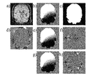
- FIGS. 3 a -3 k are exemplary images showing validation in numerical simulation.
- a numerical brain phantom is shown in a prescribed field of view (FOV) in coronal view with the simulated total field (a), the corresponding reference background field (b), the reference local field with annotated hemorrhage (H) and veins (V) (c) and the defined region of interest (ROI) (white area) (d).
- the projection onto dipole fields (PDF) method was used to estimate the background susceptibility distribution (e).
- the PDF-estimated background field (f), the PDF-estimated local field (g) and the corresponding difference from the reference (h) showed substantial improvement over the high-pass filtering (HPF) method (i, j and k, corresponding to HPF-estimated background field, HPF-estimated local field and difference from the reference, respectively).
- HPF high-pass filtering
- the relative errors were 23.51% and 3.21% for the HPF and PDF methods, respectively.
- the black box in (a) indicates the region in which the attenuation of the local field was measured.
- FIGS. 4 a -4 k are exemplary images showing validation in phantom MRI. Acquired three-dimensional data are shown in a coronal section with the total field (a), the corresponding reference background field (b), the reference local field (c) and the magnitude image (d) [with the large circular disk as the region of interest (ROI)].
- PDF projection onto dipole fields
- the PDF-estimated background field (f), the PDF-estimated local field (g) and the corresponding difference from the reference (h) showed substantial improvement over the high-pass filtering (HPF) method (i, j and k, corresponding to HPF-estimated background field, HPF-estimated local field and the difference from the reference, respectively).
- HPF high-pass filtering
- the relative errors were 18.36% and 5.53% for the HPF and PDF methods, respectively.
- the black box in (a) indicates the region in which the attenuation of the local field was measured.
- FIGS. 5 a -5 h are exemplary images showing patient brain imaging. Acquired three-dimensional data are shown in a coronal section with the magnitude image (a), the total field (b) and the region of interest (ROI) (white region) (c).
- FIG. 5( d ) shows estimated background susceptibility distribution using the projection onto dipole fields (PDF) method.
- FIGS. 5( e, f ) show background and local fields estimated by the PDF method.
- FIGS. 5( g, h ) show background and local fields estimated by the high-pass filtering (HPF) method.
- the estimated local field generated by the PDF method provides better depiction of the hemorrhage (black arrows), with a higher visual contrast between the hemorrhage and the surrounding tissue and with less artifacts (white arrow).
- FIG. 1 a block diagram of an exemplary MR system 100 for implementing embodiments of the invention is shown.
- the exemplary system includes a computer 102 , a magnet system 104 , a data acquisition system 106 , and display 108 .
- the computer 102 controls the gradient and RF magnets or coils (not shown) in the magnet system 104 via amplifiers (not shown) that transmit control signals.
- the computer 102 also controls the data acquisition system 106 that receives signals received by receiver coils (not shown), processes the data acquired, and outputs an image to display 108 .
- Computer 102 typically includes a variety of computer readable media.
- Computer readable media can be any available media that can be accessed by computer 102 and includes both volatile and nonvolatile media, removable, and non-removable media. It will be appreciated that certain embodiments of the invention may be described in the general context of computer-executable instructions, such as program modules, being executed by a computer such as a personal computer. The invention may also be practiced in distributed computing environments where tasks are performed by remote processing devices that are linked through a communications network.
- PDF projection onto dipole fields
- the method is nonparametric.
- Our data demonstrate that this nonparametric background removal technique, PDF, is successful in removing the background field, whilst allowing an accurate estimation of the local field.
- the PDF method estimates the background fields with smaller errors and results in less attenuation of the local field with respect to the reference scan method in a numerical simulation and a phantom experiment.
- the PDF method provides superior local field maps for in vivo brain imaging with less artifacts near tissue-air boundaries and more contrast in local fields induced from different brain structures.
- the HPF method performs background removal using the Fourier basis.
- the HPF method does not distinguish the source of the slowly varying components of the total field, either from the background or from the ROI.
- HPF suffers when there are overlaps between the Fourier spectra of the background and local fields.
- the background field may contain high-spatial-frequency components and the local field may contain low-spatial-frequency components. Consequently, the HPF method may fail to remove the high-spatial-frequency components of the background field near air-tissue boundaries in brain imaging ( FIG. 5 h , white arrow), and may erroneously remove the low-spatial-frequency components of the local field (as demonstrated in FIG.
- the HPF method might not be suitable for the visualization of local fields of large brain structures, such as basal ganglia or hemorrhage, and brain structures near the brain ROI boundary.
- the results of the HPF method depend on the choice of the kernel size (see Wang (2000); Langham (2009); Wharton (2010). An increase in the kernel size can improve the removal of the unwanted background field, but at the cost of attenuating the local field.
- the separation between local and background fields may be fundamentally explained by the Maxwell equation, which states that the field generated by the background dipoles is a harmonic function inside the ROI, but the field generated by the local dipoles is nonharmonic (see Li L, Leigh J S. (2001) High-precision mapping of the magnetic field utilizing the harmonic function mean value property. J. Magn. Reson. 148(2): 442-448 (“Li (2001)”)). Therefore, the background and local fields may be separable in an ideal harmonic function space. In the PDF method, the estimated background field generated by background dipoles is guaranteed to be a harmonic function. In comparison, the estimated background field by the HPF method may violate the harmonic condition.
- the PDF performance may be further improved by means such as dilating the ROI by a few voxels to convert voxels near the original ROI boundary into interior points of the enlarged ROI.
- the Fourier aliasing in FIG. 3 e (visible as the two white regions near the top of the FOV) is not a problem: its presence effectively modeled the background field at the bottom of the FOV that was, in reality, caused by susceptibility sources further below the FOV.
- the local field f L is defined as the magnetic field generated by the susceptibility distribution ⁇ L inside an ROI M
- the background field f B is defined as the magnetic field generated by the susceptibility distribution ⁇ B in the region M , which is outside the ROI and inside a sufficiently large FOV.
- the background field extends into the ROI, just as the local field extends outside the ROI.
- tissue susceptibility satisfies
- d is the unit dipole field, which is the magnetic field created by a unit dipole at the origin with the Lorentz sphere correction (see Li (2004); Haacke E M, Brown R W, Thompson M R. (1999) Objects in external fields: the Lorentz sphere. Magnetic Resonance Imaging: Physical Principles and Sequence Design. Wiley-Liss: New York, pp. 749-757 (“Haacke (1999)”); Jackson (1999)).
- our PDF method is to project the total field measured in the ROI onto the subspace spanned by the background unit dipole fields.
- the total field measured in the ROI may be used. All the background unit dipole fields may be used. This is related to the projection theorem in Hilbert space—as described in Moon T K, Stirling W C, “Pseudoinverses and the SVD. Mathematical Methods and Algorithms for Signal Processing,” Prentice Hall: Upper Saddle River, N.J., pp. 116-117 (2000) (“Moon (2000)”), which is incorporated herein by reference in its entirety—which we review briefly here.
- T be an inner product space spanned by all unit dipole responses ⁇ d r
- d r denotes the magnetic field induced by a unit dipole located at r.
- the total field f f ⁇ T.
- the inner product between any f 1 , f 2 ⁇ T is defined as the sum of element-wise multiplication between f 1 and f 2 inside the ROI only.
- the background field component f B is formed of basis functions ⁇ d rB
- the subspace spanned by all the background unit dipole fields is then denoted as B.
- the basis functions of the local field component f L are ⁇ d rL
- Orthogonality requires that, for each given local unit dipole field, its inner product with any possible background unit dipole field is zero.
- the PDF method was performed on a simulated total field consisting of a single local unit dipole field d rL , r ⁇ M and a zero background field to generate an estimated background field f* b,rL .
- the true background field is zero and, therefore, the PDF method should ideally not remove any part of the local field.
- This relative error is visualized for every voxel r inside the ROI in FIG. 2 d - f . It is observed that the error is low (E ⁇ 0.1) for dipoles located at most of the voxels in the ROI, and increases for dipoles near the boundary of the ROI.
- the computation of the total field f from MR phase data was based on phase data from multiple echo data—as described in de Rochefort (2008b), which is incorporated herein by reference in its entirety—followed by a magnitude image-guided unwrapping algorithm—as described in Cusack R, Papadakis N. (2002) New robust 3-D phase unwrapping algorithms: application to magnetic field mapping and undistorting echoplanar images. Neuroimage 16(3 Pt 1):754-764 (“Cusack (2002)”), which is incorporated herein by reference in its entirety.
- Equation [2] We accounted for spatial variations of noise in the MR field maps by adding a weight to Equation [2] to normalize the noise to a normal distribution N(0,1).
- the weight w was derived from magnitude images across multiple echoes—as described in Kressler (2009), which is incorporated herein by reference in its entirety.
- N the number of voxels in the MR image dataset, and expressed the measured total field f and the total susceptibility distribution ⁇ as N ⁇ 1 column vectors.
- I an N ⁇ N identity matrix
- M an N ⁇ N diagonal matrix, where the diagonal elements are equal to unity when they correspond to voxels inside the ROI and are equal to zero otherwise.
- ⁇ B (I ⁇ M) ⁇ .
- D denotes an N ⁇ N matrix representing the convolution with the unit dipole field d
- W denotes an N ⁇ N diagonal matrix formed by placing the weighting w on the diagonal.
- Equation [5] A fast calculation method for magnetic field inhomogeneity due to an arbitrary distribution of bulk susceptibility.
- Concept Magn Reson B 19B(1):26-34 (“Salomir (2003)”)).
- the PDF method was compared with the HPF method that has been commonly used in the literature.
- HPF a three-dimensional Hann window low-pass filter with a kernel size of 32 ⁇ 32 ⁇ 32 was applied to the complex MRI data when one echo was used (see Wang (2000)).
- the low-pass filter was applied to a reconstructed complex MRI dataset formed by setting the magnitude equal to that of the first echo and the phase equal to the unwrapped total field normalized to [ ⁇ , ⁇ ).
- the background field was estimated from the phase of the resulting low-pass-filtered complex image. All the algorithms were implemented on a personal computer with Intel® CoreTM i7 CPU, 6-GB memory using MATLAB (2009a) code (MathWorks, Natick, Mass., USA).
- An ellipsoid whose radii were 40, 40 and 54 voxels was created in a 160 ⁇ 160 ⁇ 160 matrix to imitate the shape of a head.
- Five smaller ellipsoids were created inside the head-shaped ellipsoid to simulate mastoid cavities, ethmoid and maxillary sinuses. The radii of these ellipsoids ranged from 10 to 15 voxels.
- Three cylinders with a radius of two voxels and a length of 20 voxels were created to simulate veins and were placed inside the head-shaped ellipsoid along the x, y and z directions, respectively.
- a sphere with a radius of five voxels was created in the mid-brain to mimic a hemorrhage.
- Complex MRI data were simulated from this geometry.
- a uniform intensity of 100 was assigned to the ‘head’ region, and the ‘air’ cavities were assigned a value of zero.
- Susceptibility in the ‘head’ region was chosen to be the zero reference, the susceptibility of ‘air’ was 9.4 ppm (see de Rochefort (2008)), the vessels were 0.3 ppm (see Fernandez-Seara (2006)), and the hemorrhage was 1.2 ppm (see de Rochefort L, Liu T, Kressler B, Liu J, Spincemaille P, Wu J, Wang Y.
- relative errors of the background field were calculated to assess the goodness of the background removal.
- Relative errors were calculated by taking the noun of the difference between the estimated background field and the reference background field, and then normalized by the norm of the reference background field.
- the norms were calculated inside the ROI only.
- the attenuation of the local field as a result of the background removal processes was calculated as one minus the ratio between the norm of the estimated local field and the noun of the reference local field.
- the norms were calculated inside a manually defined rectangular volume comprising the susceptibility sources of interest to capture the local attenuation of the local field, whilst ignoring the amplification elsewhere, e.g. near the boundary of the ROI.
- FIG. 3 The results of the numerical simulation are shown in FIG. 3 .
- the PDF method successfully removed the background field, leaving the local fields from ‘veins’ and ‘hemorrhage’ intact, leading to the distinct dipole pattern in the local field ( FIG. 3 g ).
- FIG. 3 h There was little discernible visual difference between the local field estimated by the PDF method and the reference local field ( FIG. 3 h ).
- HPF left substantial residual background field in regions close to the ‘ethmoid sinus’ and ‘mastoid cavities’ ( FIG. 3 j ), and removed indiscriminately the slowly varying component of the field induced by the ‘hemorrhage’ ( FIG. 3 i, k , arrows).
- the relative errors between the estimated and reference background fields were 23.51% and 3.21% for the HPF and PDF methods, respectively, and the attenuations of the local fields were 41.1% and 1.2%, respectively.
- the CG algorithm of the PDF method converged with 10 iterations in 0.7 s.
- a cylindrical water phantom (diameter, 10 cm; height, 8.5 cm) was constructed.
- Three vials (diameter, 1.2 cm; height, 6 cm) with 1% concentrated gadolinium (Gd; Magnevist, Berlex Laboratories, Wayne, N.J., USA) were placed vertically in the water container to mimic three vessels.
- a waterproof plastic air box (2.5 ⁇ 2.5 ⁇ 1.5 cm 3 ) was glued to the bottom of the water container to imitate an air cavity.
- the phantoms were scanned on a 1.5-T clinical MRI scanner (General Electric Excite HD; GE Healthcare, Waukesha, Wis., USA) using a 5-in surface coil for signal reception.
- a dedicated three-dimensional gradient-echo sequence was designed to sample at different TEs in an interleaved manner.
- Four TEs (1.7, 2.2, 4.2 and 14.2 ms) were used to achieve a balance between the precision of the estimated total field and the total scan time. After this scan had been completed, the three vials were removed from the water phantom. The scan was repeated with identical imaging parameters to acquire a reference background field. The scanner gradient shimming was kept constant between the two scans.
- the background air region without MR signal was segmented as M (background black region in FIG. 4 d ), and the rest was denoted as M. Noise was estimated from M . Similar to the numerical simulation, estimated background fields were compared qualitatively and quantitatively with the reference background field.
- the results for the phantom experiment are shown in FIG. 4 .
- the estimated background field by the PDF method was in good agreement with the reference background field ( FIG. 4 h ), whereas the estimated background field by the HPF method contained a substantial amount of the local field ( FIG. 4 i, k , arrow).
- the relative errors between the estimated and reference background fields were 18.36% and 5.53% for the HPF and PDF methods, respectively, and the attenuations of the local fields were 43.0% and 3.2%, respectively.
- the CG algorithm of the PDF method converged with 43 iterations in 17.0 s.
- the phase images were used to fit the total field.
- the brain region was segmented and denoted as the ROI M, and the remaining regions in the imaging volume were considered to comprise M .
- Estimated background fields were obtained and removed using both techniques.
- the three-dimensional brain data was reformatted to coronal sections for inspection.
- field contrasts were calculated from PDF and HPF processed field maps. Rectangular volumes immediately superior to the hemorrhages and volumes on the right of the hemorrhages were drawn, and the differences between the mean values insides these two regions were calculated. These two regions fall inside two lobes of the dipole field that have opposite sign.
- the resulting contrast measurements were compared between the HPF and PDF methods over the 15 patients using a two-tailed paired t-test with a significance level p of 0.01.
- the estimated local field by the HPF method contained substantially more field variation at the periphery of the brain ROI, which might be interpreted as high-spatial-frequency residual background field because of the air-tissue interface ( FIG. 5 h , white arrow).
- the local fields arising from the hemorrhagic lesion estimated by the PDF method were stronger than those estimated by the HPF method (black arrows), resulting in a better contrast in the field maps between the hemorrhage and the surrounding tissue by the PDF method.
- the PDF-processed image showed higher field contrast than the HPF-processed image for each of the 15 cases (21 ⁇ 8 Hz versus 12 ⁇ 5 Hz, p ⁇ 0.001).
Abstract
Description
f=f L +f B =d
argmin χBε
0≦c(r L)=maxr
χB*=argminχB ∥w(f−d
where the norm ∥•∥2 in Equation [4] is again calculated only over the ROI M, which may be defined using image segmentation, and the dot symbol indicates point-wise multiplication between vectors.
MWD(I−M)χ=MWf [5]
A H Aχ=A Hβ [6]
where β=MWf. The CG iteration was stopped when the norm of the residual was smaller than 50% of the expected noise level ∥AHMu∥2, where u was a column vector containing ones. Once χ* had been estimated, the background field was calculated as:
f B *=Dχ R *=D(I−M)χ* [7]
and was subtracted from the measured total field f to estimate the local field C.
Comparison with High-Pass Filtering (HPF)
-
- Liu J, Liu T, de Rochefort L, Ledoux J, Khalidov I, Chen W, Tsiouris A J, Wisnieff C, Spincemaille P, Prince M R, Wang Y., Morphology enabled dipole inversion for quantitative susceptibility mapping using structural consistency between the magnitude image and the susceptibility map. Neuroimage. 2011 Sep. 8. [Epub ahead of print]
- Liu T, Liu J, de Rochefort L, Spincemaille P, Khalidov I, Ledoux J R, Wang Y., Morphology enabled dipole inversion (MEDI) from a single-angle acquisition: comparison with COSMOS in human brain imaging. Magn Reson Med. 2011 September; 66(3):777-83. doi: 10.1002/mrm.22816. Epub 2011 Apr. 4.
- Liu T, Khalidov I, de Rochefort L, Spincemaille P, Liu J, Tsiouris A J, Wang Y., A novel background field removal method for MRI using projection onto dipole fields (PDF). NMR Biomed. 2011 November; 24(9):1129-36.
- Liu T, Spincemaille P, de Rochefort L, Wong R, Prince M, Wang Y. m Unambiguous identification of superparamagnetic iron oxide particles through quantitative susceptibility mapping of the nonlinear response to magnetic fields. Magn Reson Imaging. 2010 November; 28(9):1383-9.
Claims (14)
Priority Applications (1)
| Application Number | Priority Date | Filing Date | Title |
|---|---|---|---|
| US13/304,141 US9448289B2 (en) | 2010-11-23 | 2011-11-23 | Background field removal method for MRI using projection onto dipole fields |
Applications Claiming Priority (2)
| Application Number | Priority Date | Filing Date | Title |
|---|---|---|---|
| US41669610P | 2010-11-23 | 2010-11-23 | |
| US13/304,141 US9448289B2 (en) | 2010-11-23 | 2011-11-23 | Background field removal method for MRI using projection onto dipole fields |
Publications (2)
| Publication Number | Publication Date |
|---|---|
| US20120141003A1 US20120141003A1 (en) | 2012-06-07 |
| US9448289B2 true US9448289B2 (en) | 2016-09-20 |
Family
ID=46162285
Family Applications (1)
| Application Number | Title | Priority Date | Filing Date |
|---|---|---|---|
| US13/304,141 Active 2033-10-20 US9448289B2 (en) | 2010-11-23 | 2011-11-23 | Background field removal method for MRI using projection onto dipole fields |
Country Status (1)
| Country | Link |
|---|---|
| US (1) | US9448289B2 (en) |
Cited By (11)
| Publication number | Priority date | Publication date | Assignee | Title |
|---|---|---|---|---|
| US20140312896A1 (en) * | 2011-04-22 | 2014-10-23 | Klaas Prussmann | Observation of Axial Magnetization of an Object in a Magnetic Field |
| US20180372826A1 (en) * | 2015-12-17 | 2018-12-27 | Koninklijke Philips N.V. | Segmentation of quantitative susceptibility mapping magnetic resonance images |
| US10638951B2 (en) | 2018-07-06 | 2020-05-05 | Shanghai United Imaging Healthcare Co., Ltd. | Systems and methods for magnetic resonance imaging |
| US11051695B2 (en) | 2017-09-11 | 2021-07-06 | Hitachi, Ltd. | Magnetic resonance imaging apparatus |
| US11273283B2 (en) | 2017-12-31 | 2022-03-15 | Neuroenhancement Lab, LLC | Method and apparatus for neuroenhancement to enhance emotional response |
| US11364361B2 (en) | 2018-04-20 | 2022-06-21 | Neuroenhancement Lab, LLC | System and method for inducing sleep by transplanting mental states |
| US11452839B2 (en) | 2018-09-14 | 2022-09-27 | Neuroenhancement Lab, LLC | System and method of improving sleep |
| US11717686B2 (en) | 2017-12-04 | 2023-08-08 | Neuroenhancement Lab, LLC | Method and apparatus for neuroenhancement to facilitate learning and performance |
| US11723579B2 (en) | 2017-09-19 | 2023-08-15 | Neuroenhancement Lab, LLC | Method and apparatus for neuroenhancement |
| US11786694B2 (en) | 2019-05-24 | 2023-10-17 | NeuroLight, Inc. | Device, method, and app for facilitating sleep |
| US11940519B2 (en) | 2021-04-21 | 2024-03-26 | Siemens Healthineers Ag | Method and system for determining a magnetic susceptibility distribution |
Families Citing this family (8)
| Publication number | Priority date | Publication date | Assignee | Title |
|---|---|---|---|---|
| US11324413B1 (en) | 2013-03-13 | 2022-05-10 | Center For Neurological Studies | Traumatic brain injury diffusion tensor and susceptibility weighted imaging |
| US11146903B2 (en) | 2013-05-29 | 2021-10-12 | Qualcomm Incorporated | Compression of decomposed representations of a sound field |
| US9922656B2 (en) | 2014-01-30 | 2018-03-20 | Qualcomm Incorporated | Transitioning of ambient higher-order ambisonic coefficients |
| US10770087B2 (en) | 2014-05-16 | 2020-09-08 | Qualcomm Incorporated | Selecting codebooks for coding vectors decomposed from higher-order ambisonic audio signals |
| CN104107045B (en) * | 2014-06-30 | 2016-08-17 | 沈阳东软医疗系统有限公司 | MR imaging method and device |
| CN106999091B (en) * | 2014-12-04 | 2020-12-01 | 通用电气公司 | Method and system for improved classification of constituent materials |
| WO2018050627A1 (en) * | 2016-09-13 | 2018-03-22 | Institut National De La Sante Et De La Recherche Medicale (Inserm) | A method for post-processing liver mri images to obtain a reconstructed map of the internal magnetic susceptibility |
| JP2020146286A (en) * | 2019-03-14 | 2020-09-17 | 株式会社リコー | Information processing device, information processing method, program and biological signal measurement system |
Citations (2)
| Publication number | Priority date | Publication date | Assignee | Title |
|---|---|---|---|---|
| US20110044524A1 (en) * | 2008-04-28 | 2011-02-24 | Cornell University | Tool for accurate quantification in molecular mri |
| US20130221961A1 (en) * | 2012-02-27 | 2013-08-29 | Medimagemetric LLC | System, Process and Computer-Accessible Medium For Providing Quantitative Susceptibility Mapping |
-
2011
- 2011-11-23 US US13/304,141 patent/US9448289B2/en active Active
Patent Citations (2)
| Publication number | Priority date | Publication date | Assignee | Title |
|---|---|---|---|---|
| US20110044524A1 (en) * | 2008-04-28 | 2011-02-24 | Cornell University | Tool for accurate quantification in molecular mri |
| US20130221961A1 (en) * | 2012-02-27 | 2013-08-29 | Medimagemetric LLC | System, Process and Computer-Accessible Medium For Providing Quantitative Susceptibility Mapping |
Non-Patent Citations (69)
| Title |
|---|
| "Hilbert space", Feb. 7, 2010, Wikipedia.org, p. 7-8. * |
| Akbudak, et al., Contrast-Agent Phase Effects: An Experimental System for Analysis of Susceptibility, Concentration, and Bolus Input Function Kinetics, Magn Reson Med, 38: 990-1002 (1997). |
| Albert, et al, Susceptibility Changes Following Bolus Injections, Magn Reson Med, 29: 700-708 (1993). |
| Ben-Israel et al., Generalized inverses, theory and applications, 2nd edition, Society CM, editor, New York: Springer, p. 118-122 (2000). |
| Beutler, et al., Iron Deficiency and Overload, Hematol Am Soc Hematol Educ Program, p. 40-61 (2003). |
| Björck, Iterative methods for least squares problems. Numerical Methods for Least Squares Problems, Society for Industrial Mathematics: Philadelphia, Pennsylvania, pp. 269-270, 290-292 (1996). |
| Chu, et al., MRI Measurement of Hepatic Magnetic Susceptibility-Phantom Validation and Normal Subject Studies, Magn Reson in Med. 52: 1318-1327 (2004). |
| Collins et al., Numerical calculations of the static magnetic field in three-dimensional multi-tissue models of the human head, Magn Reson Imaging, 20: 413-424 (2002). |
| Conturo et al., Signal-to-Noise in Phase Angle Reconstruction: Dynamic Range Extension Using Phase Reference Offsets, Magn Reson Med, 15: 420-437 (1990). |
| Corot et al, Recent advances in iron oxide nanocrystal technology for medical imaging,Adv Drug Deliv Rev, 58: 1471-1504 (2006). |
| Cusack, et al., New robust 3-D phase unwrapping algorithms: application to magnetic field mapping and undistorting echoplanar images. Neuroimage 16(3 Pt 1): 754-764 (2002). |
| de Rochefort et al., "Quantitative susceptibility map reconstruction from MR phase data using bayesian regularization: Validation and application to brain imaging", Dec. 1, 2009, Wiley-Liss, Magnetic Resonance in Medicine, vol. 63, iss. 1, p. 194-206. * |
| De Rochefort, et al. Quantitative susceptibility map reconstruction from MR phase data using bayesian regularization: validation and application to brain imaging. Magn. Reson. Med. 63(1): 194-206 (2010). |
| De Rochefort, et al., A Weighted Gradient Regularization Solution to the Inverse Problem from Magnetic Field to Susceptibility Maps (Magnetic Source MRI): Validation and Application to Iron Quantification in the Human Brain. Proc ISMRM 462 (2009). |
| De Rochefort, et al., In vivo quantification of contrast agent concentration using the induced magnetic field for time-resolved arterial input function measurement with MRI. Medical physics 35(12): 5328-5339 (2008). |
| De Rochefort, et al., Quantitative MR susceptibility mapping using piece-wise constant regularized inversion of the magnetic field, Magn Reson Med; 60(4): 1003-1009 (2009). |
| Dias et al, the ZpiM Algorithm: A Method for Interferometric Image Reconstruction in SAR/SAS, IEEE Trans Image Processing, 11(4): 408-422 (2002). |
| Fernandez-Seara, et al., MR susceptometry for measuring global brain oxygen extraction. Magn Reson Med 55(5): 967-973 (2006). |
| Gonzalez et al., Image Restoration, Digital Image Processing, Reading MA: Addison Wesley, p. 253-305 (1992). |
| Haacke, et al. Objects in external fields: the Lorentz sphere. Magnetic Resonance Imaging: Physical Principles and Sequence Design. Wiley-Liss: New York, pp. 749-757 (1999). |
| Haacke, et al., Imaging iron stores in the brain using magnetic resonance imaging. Magn. Reson. Imaging 23(1): 1-25 (2005). |
| Haacke, et al., Susceptibility weighted imaging (SWI). Magn Reson Med 52(3): 612-618 (2004). |
| Hamalainen, et al., Magnetoencephalography: theory, instrumentation, and applications to noninvasive studies of the working human brain, Reviews of Modern Physics, 65: 413-497 (1993). |
| Hestenes et al., Methods of Conjugate Gradients for Solving Linear Systems, J Research Natl Bureau Standards, 49(6): 409-436 (1952). |
| Hoffman, Measurement of magnetic susceptibility and calculation of shape factor of NMR samples, J Magnetic Resonance, 178: 237-247 (2006). |
| Holt et al., MR Susceptometry: an External-Phantom Method for Measuring Bulk Susceptibility from Field-Echo Phase Reconstruction Maps, Magn Reson Imaging, 4: 809-818 (1994). |
| Hopkins et al., Magnetic Susceptibility Measurement of Insoluble Solids by NMR: Magnetic Susceptibility of Bone, Magn Reson Med 37: 494-500 (1997). |
| Jackson, et al., Classical electrodynamics, third edition: John Wiley and Sons, inc., pp. 184-188 (1999). |
| Kahn, Molecular Magnetism, Weiheim: Wiley-VCH, pp. 9-10 (1993). |
| Koch, et al. , Rapid calculations of susceptibility-induced magnetostatic field perturbations for in vivo magnetic resonance. Physics in medicine and biology 51(24):6381-6402 (2006). |
| Kressler, et al., Nonlinear Regularization for Per Voxel Estimation of Magnetic Susceptibility Distributions from MRI Field Maps. IEEE transactions on medical imaging (2009). |
| Langham, et al. Retrospective correction for induced magnetic field inhomogeneity in measurements of large-vessel hemoglobin oxygen saturation by MR susceptometry. Magn Reson Med 61(3): 626-633 (2009). |
| Lee et al., Cerebral microbleeds are a risk factor for warfarin-related intracerebral hemorrhage, Neurology, 72: 171-176 (2009). |
| Li et al. , Magnetic susceptibility quantitation with MRI by solving boundary value problems, Med Phys, 30(3): 449-453 (2003). |
| Li et al., Accounting for Signal Loss Due to Dephasing in the Correction of Distortions in Gradient-Echo EPI Via Nonrigid Registration, IEEE Trans Med Imaging, 26(12): 1698-1707 (2007). |
| Li et al., Magnetic Susceptibility Quantification for Arbitrarily Shaped Objects in Inhomogeneous Fields, Magn Reson in Med, 46: 907-916 (2001). |
| Li, et al., High-precision mapping of the magnetic field utilizing the harmonic function mean value property. J. Magn. Reson. 148(2): 442-448 (2001). |
| Li, et al., Quantifying arbitrary magnetic susceptibility distributions with MR. Magnet Reson Med 51(5): 1077-1082 (2004). |
| Liu, et al., A novel background field removal method for MRI using projection onto dipole fields (PDF). NMR Biomed.; 24(9): 1129-36 (Nov. 2011). |
| Liu, et al., Calculation of susceptibility through multiple orientation sampling (COSMOS): a method for conditioning the inverse problem from measured magnetic field map to susceptibility source image in MRI. Magn Reson Med 61(1): 196-204 (2009). |
| Liu, et al., Morphology enabled dipole inversion (MEDI) from a single-angle acquisition: comparison with COSMOS in human brain imaging. Magn Reson Med. ;66(3): 777-83 (Sep. 2011). |
| Liu, et al., Morphology enabled dipole inversion for quantitative susceptibility mapping using structural consistency between the magnitude image and the susceptibility map. Neuroimage. (Sep. 8, 2011). |
| Liu, et al., Unambiguous identification of superparamagnetic iron oxide particles through quantitative susceptibility mapping of the nonlinear response to magnetic fields. Magn Reson Imaging. 28(9):1383-9 (Nov. 2010). |
| Marques, et al., Application of a Fourier-based method for rapid calculation of field inhomogeneity due to spatial variation of magnetic susceptibility. Concepts in Magnetic Resonance Part B: Magnetic Resonance Engineering 258(1):65-78 (2005). |
| Moon, et al., Pseudoinverses and the SVD. Mathematical Methods and Algorithms for Signal Processing, Prentice Hall: Upper Saddle River, New Jersey, pp. 116-117 (2000). |
| Morgan et al, Efficient solving for arbitrary susceptibility distributions using residual difference fields, Proceedings of the 15th Annual Meeting of the ISMRM, Berlin, p. 35 (2007). |
| Neelavalli, et al., Removing background phase variations in susceptibility-weighted imaging using a fast, forward-field calculation. J Magn Reson Imaging 29(4):937-948 (2009). |
| Salomir, et al., A fast calculation method for magnetic field inhomogeneity due to an arbitrary distribution of bulk susceptibility. Concept Magn Reson B 19B(1):26-34 (2003). |
| Schabel et al., Uncertainty and bias in contrast concentration measurements using spoiled gradient echo pulse sequences, Phys Med Biol, 53: 2345-2373 (2008). |
| Schweser et al, A Novel Approach for Separation of Background Phase in SWI Phase Data Utilizing the Harmonic Function Mean Value Property, Stockholm, Sweden, Proc Intl Soc Magn Reson Med, p. 142 (2010). |
| Sekihara et al., "Noise Covariance Incorporated MEG-MUSIC Algorithm: A Method for Multiple-Dipole Estimation Tolerant of the Influence of Background Brain Activity", Sep. 9, 1997, IEEE Transactions on Biomedical Engineering, vol. 44, No. 9, p. 839-847. * |
| Sepulveda et al., Magnetic Susceptibility Tomography for Three-Dimensional Imaging of Diamagnetic and Paramagnetic Objects, IEEE Transactions on Magnetics, 30(6): 5062-5069 (1994). |
| Shmueli, et al., Magnetic susceptibility mapping of brain tissue in vivo using MRI phase data. Magn. Reson. Med. 62(6): 1510-1522 (2009). |
| Smirnov et al., In Vivo Single Cell Detection of Tumor-Infiltrating Lymphocytes With a Clinical 1.5 Tesla MRI System, Magn Reson in Med, 60: 1292-1297 (2008). |
| Stanisz et al., Gd-DTPA Relaxivity Depends on Macromolecular Content, Magn Reson in Med, 44: 665-667 (2000). |
| Stark et al., Hemorrhage, Magnetic resonance imaging, vol. III, 3rd ed, St. Louis, p. 1329-1345 (1999). |
| Terreno et al., Effect of the Intracellular Localization of a Gd-Based Imaging Probe on the Relaxation Enhancement of Water Protons, Magn Reson in Med, 55: 491-497 (2006). |
| Truong et al., Three-dimensional numerical simulations of susceptibility-induced magnetic field inhomogeneities in the human head, Magn Reson Imaging, 20: 759-770 (2002). |
| Wang et al., Magnetic Resonance Imaging Measurement of Volume Magnetic Susceptibility Using a Boundary Condition, J Magn Reson, 140: 477-481 (1999). |
| Wang, et al., Artery and vein separation using susceptibility-dependent phase in contrast-enhanced MRA. J Magn Reson Imaging 12(5): 661-670 (2000). |
| Weisskoff, et al., MRI Susceptometry: Image-Based Measurement of Absolute Susceptibility of MR Contrast Agents and Human Blood, Magn Reson in Med. 24: 375-383 (1992). |
| Wharton, et al., Susceptibility mapping in the human brain using threshold-based k-space division. Magn. Reson. Med. 63(5): 1292-1304 (2010). |
| Wickline et al. , Molecular Imaging and Therapy of Atherosclerosis With Targeted Nanoparticles, J Magn Reson Imaging, 25: 667-680 (2007). |
| Wu et al. Identification of Calcification with MRI Using Susceptibility-Weighted Imaging: A Case Study, J Magn Reson Imaging, 29: 177-182 (2009). |
| Yablonskiy et al., Theory of NMR signal Behavior in Magnetically Inhomogeneous Tissues: The Static Dephasing Regime, Magn Reson Med, 32: 749-763 (1994). |
| Yao, et al., Susceptibility contrast in high field MRI of human brain as a function of tissue iron content, Neuroimage 44:1259-1266 (2009). |
| Yao, et al., Susceptibility contrast in high field MRI of human brain as a function of tissue iron content. Neuroimage 44(4):1259-1266 (2009). |
| Zhong et al., The molecular basis for gray and white matter contrast in phase imaging, Neuroimage, 40: 1561-1566 (2008). |
| Zurkiya et al, MagA is Sufficient for Producing Magnetic Nanoparticles in Mammalian Cells, Making it an MRI Reporter, Magn Reson in Med, 59: 1225-1231 (2008). |
Cited By (15)
| Publication number | Priority date | Publication date | Assignee | Title |
|---|---|---|---|---|
| US9733318B2 (en) * | 2011-04-22 | 2017-08-15 | Eidgenossische Technische Hochschule (Eth) | Observation of axial magnetization of an object in a magnetic field |
| US20140312896A1 (en) * | 2011-04-22 | 2014-10-23 | Klaas Prussmann | Observation of Axial Magnetization of an Object in a Magnetic Field |
| US20180372826A1 (en) * | 2015-12-17 | 2018-12-27 | Koninklijke Philips N.V. | Segmentation of quantitative susceptibility mapping magnetic resonance images |
| US10761170B2 (en) * | 2015-12-17 | 2020-09-01 | Koninklijke Philips N.V. | Segmentation of quantitative susceptibility mapping magnetic resonance images |
| US11051695B2 (en) | 2017-09-11 | 2021-07-06 | Hitachi, Ltd. | Magnetic resonance imaging apparatus |
| US11723579B2 (en) | 2017-09-19 | 2023-08-15 | Neuroenhancement Lab, LLC | Method and apparatus for neuroenhancement |
| US11717686B2 (en) | 2017-12-04 | 2023-08-08 | Neuroenhancement Lab, LLC | Method and apparatus for neuroenhancement to facilitate learning and performance |
| US11273283B2 (en) | 2017-12-31 | 2022-03-15 | Neuroenhancement Lab, LLC | Method and apparatus for neuroenhancement to enhance emotional response |
| US11318277B2 (en) | 2017-12-31 | 2022-05-03 | Neuroenhancement Lab, LLC | Method and apparatus for neuroenhancement to enhance emotional response |
| US11478603B2 (en) | 2017-12-31 | 2022-10-25 | Neuroenhancement Lab, LLC | Method and apparatus for neuroenhancement to enhance emotional response |
| US11364361B2 (en) | 2018-04-20 | 2022-06-21 | Neuroenhancement Lab, LLC | System and method for inducing sleep by transplanting mental states |
| US10638951B2 (en) | 2018-07-06 | 2020-05-05 | Shanghai United Imaging Healthcare Co., Ltd. | Systems and methods for magnetic resonance imaging |
| US11452839B2 (en) | 2018-09-14 | 2022-09-27 | Neuroenhancement Lab, LLC | System and method of improving sleep |
| US11786694B2 (en) | 2019-05-24 | 2023-10-17 | NeuroLight, Inc. | Device, method, and app for facilitating sleep |
| US11940519B2 (en) | 2021-04-21 | 2024-03-26 | Siemens Healthineers Ag | Method and system for determining a magnetic susceptibility distribution |
Also Published As
| Publication number | Publication date |
|---|---|
| US20120141003A1 (en) | 2012-06-07 |
Similar Documents
| Publication | Publication Date | Title |
|---|---|---|
| US9448289B2 (en) | Background field removal method for MRI using projection onto dipole fields | |
| Liu et al. | A novel background field removal method for MRI using projection onto dipole fields | |
| Polimeni et al. | Analysis strategies for high-resolution UHF-fMRI data | |
| Metere et al. | Simultaneous quantitative MRI mapping of T 1, T 2* and magnetic susceptibility with multi-echo MP2RAGE | |
| Ruthotto et al. | Diffeomorphic susceptibility artifact correction of diffusion-weighted magnetic resonance images | |
| Avram et al. | Clinical feasibility of using mean apparent propagator (MAP) MRI to characterize brain tissue microstructure | |
| Schweser et al. | Quantitative susceptibility mapping for investigating subtle susceptibility variations in the human brain | |
| Li et al. | A method for estimating and removing streaking artifacts in quantitative susceptibility mapping | |
| Li et al. | Mapping magnetic susceptibility anisotropies of white matter in vivo in the human brain at 7 T | |
| Huang et al. | Body MR imaging: artifacts, k-space, and solutions | |
| Zhou et al. | Background field removal by solving the Laplacian boundary value problem | |
| De Rochefort et al. | Quantitative MR susceptibility mapping using piece‐wise constant regularized inversion of the magnetic field | |
| Sun et al. | Quantitative susceptibility mapping using a superposed dipole inversion method: application to intracranial hemorrhage | |
| Bock et al. | Optimizing T1-weighted imaging of cortical myelin content at 3.0 T | |
| Wen et al. | An iterative spherical mean value method for background field removal in MRI | |
| Li et al. | Mean magnetic susceptibility regularized susceptibility tensor imaging (MMSR‐STI) for estimating orientations of white matter fibers in human brain | |
| US20130343625A1 (en) | System and method for model consistency constrained medical image reconstruction | |
| Koolstra et al. | Cartesian MR fingerprinting in the eye at 7T using compressed sensing and matrix completion‐based reconstructions | |
| Tabelow et al. | Local estimation of the noise level in MRI using structural adaptation | |
| Liu et al. | Imaging neural architecture of the brain based on its multipole magnetic response | |
| Cai et al. | Single-Shot ${\text {T}} _ {{2}} $ Mapping Through OverLapping-Echo Detachment (OLED) Planar Imaging | |
| Fang et al. | Background field removal using a region adaptive kernel for quantitative susceptibility mapping of human brain | |
| Liang et al. | A variable flip angle-based method for reducing blurring in 3D GRASE ASL | |
| Lim et al. | Quantitative magnetic susceptibility mapping without phase unwrapping using WASSR | |
| Kan et al. | Quantitative susceptibility mapping using principles of echo shifting with a train of observations sequence on 1.5 T MRI |
Legal Events
| Date | Code | Title | Description |
|---|---|---|---|
| AS | Assignment |
Owner name: CORNELL UNIVERSITY, NEW YORK Free format text: ASSIGNMENT OF ASSIGNORS INTEREST;ASSIGNORS:WANG, YI;DE ROCHEFORT, LUDOVIC;LIU, TIAN;AND OTHERS;SIGNING DATES FROM 20120106 TO 20120120;REEL/FRAME:027703/0475 |
|
| STCF | Information on status: patent grant |
Free format text: PATENTED CASE |
|
| AS | Assignment |
Owner name: NATIONAL INSTITUTES OF HEALTH (NIH), U.S. DEPT. OF Free format text: CONFIRMATORY LICENSE;ASSIGNOR:CORNELL UNIVERSITY;REEL/FRAME:040513/0051 Effective date: 20161028 |
|
| MAFP | Maintenance fee payment |
Free format text: PAYMENT OF MAINTENANCE FEE, 4TH YR, SMALL ENTITY (ORIGINAL EVENT CODE: M2551); ENTITY STATUS OF PATENT OWNER: SMALL ENTITY Year of fee payment: 4 |
|
| MAFP | Maintenance fee payment |
Free format text: PAYMENT OF MAINTENANCE FEE, 8TH YR, SMALL ENTITY (ORIGINAL EVENT CODE: M2552); ENTITY STATUS OF PATENT OWNER: SMALL ENTITY Year of fee payment: 8 |