US9052358B2 - Copula-based system and method for management of manufacturing test and product specification throughout the product lifecycle for electronic systems or integrated circuits - Google Patents
Copula-based system and method for management of manufacturing test and product specification throughout the product lifecycle for electronic systems or integrated circuits Download PDFInfo
- Publication number
- US9052358B2 US9052358B2 US13/360,373 US201213360373A US9052358B2 US 9052358 B2 US9052358 B2 US 9052358B2 US 201213360373 A US201213360373 A US 201213360373A US 9052358 B2 US9052358 B2 US 9052358B2
- Authority
- US
- United States
- Prior art keywords
- copula
- test
- product
- data
- model
- Prior art date
- Legal status (The legal status is an assumption and is not a legal conclusion. Google has not performed a legal analysis and makes no representation as to the accuracy of the status listed.)
- Expired - Fee Related, expires
Links
Images


Classifications
-
- G—PHYSICS
- G01—MEASURING; TESTING
- G01R—MEASURING ELECTRIC VARIABLES; MEASURING MAGNETIC VARIABLES
- G01R31/00—Arrangements for testing electric properties; Arrangements for locating electric faults; Arrangements for electrical testing characterised by what is being tested not provided for elsewhere
- G01R31/28—Testing of electronic circuits, e.g. by signal tracer
- G01R31/317—Testing of digital circuits
- G01R31/31718—Logistic aspects, e.g. binning, selection, sorting of devices under test, tester/handler interaction networks, Test management software, e.g. software for test statistics or test evaluation, yield analysis
-
- G06F17/5018—
-
- G06F17/5036—
-
- G—PHYSICS
- G06—COMPUTING; CALCULATING OR COUNTING
- G06F—ELECTRIC DIGITAL DATA PROCESSING
- G06F2119/00—Details relating to the type or aim of the analysis or the optimisation
- G06F2119/06—Power analysis or power optimisation
-
- G—PHYSICS
- G06—COMPUTING; CALCULATING OR COUNTING
- G06F—ELECTRIC DIGITAL DATA PROCESSING
- G06F2119/00—Details relating to the type or aim of the analysis or the optimisation
- G06F2119/08—Thermal analysis or thermal optimisation
-
- G06F2217/78—
-
- G06F2217/80—
-
- G—PHYSICS
- G06—COMPUTING; CALCULATING OR COUNTING
- G06F—ELECTRIC DIGITAL DATA PROCESSING
- G06F30/00—Computer-aided design [CAD]
- G06F30/20—Design optimisation, verification or simulation
- G06F30/23—Design optimisation, verification or simulation using finite element methods [FEM] or finite difference methods [FDM]
-
- G—PHYSICS
- G06—COMPUTING; CALCULATING OR COUNTING
- G06F—ELECTRIC DIGITAL DATA PROCESSING
- G06F30/00—Computer-aided design [CAD]
- G06F30/30—Circuit design
- G06F30/36—Circuit design at the analogue level
- G06F30/367—Design verification, e.g. using simulation, simulation program with integrated circuit emphasis [SPICE], direct methods or relaxation methods
Definitions
- the present invention relates generally to the design and manufacturing test of electronic systems or integrated circuits. More particularly, the invention relates to a system and method that supports decision-making in the design and manufacture of electronic systems or integrated circuit components throughout the product lifecycle.
- Design and manufacturing test of electronic systems require consideration of the effect of variation of individual components on the variability of the system.
- design and manufacturing test of integrated circuit components require consideration of the effect of variation of individual circuit modules on the variation of the integrated circuit itself. Characterizing and modeling this variation support decision-making in the design and manufacturing test of both electronic systems and integrated circuit components.
- Test in the manufacture of electronic systems or integrated circuit components requires specification of test conditions such as temperatures, voltages, frequencies and parametric test limits, as well as end-use specifications. End-use specifications are given in a datasheet specification document used by designers of systems employing the electronic (sub-) system or integrated circuit component being manufactured. Test specifications and datasheet specifications are set to optimize yield, yet meet quality and reliability requirements, and so have an important revenue and brand image impact. Each unit tested is characterized by many parametric attributes such as power and delay for electronic systems, or I sb , F max , bit refresh time, reliability lifetimes, etc., for integrated circuit components, all as functions of environmental conditions such as temperature, voltage and frequency. These parametric attributes are dependent (correlated) to various degrees in the population of manufactured units.
- a traditional method of optimizing the test manufacturing flow is to characterize a sufficiently large sample of units of a specific product by measuring, but not screening, the multiple parametric attributes over a range of temperatures, voltages, and frequencies corresponding to possible Test and Use conditions of a future product. Test set points and limits are then found by filtering the data and computing figures of merit (FOMs) such as yield loss, overkill, and end-use fail fraction so that manufacturing cost, and quality and reliability targets are met. What is needed is a way to do this earlier in the product lifecycle by building a statistical model of a product from test vehicle data and then using the model to scale the model to the specific die area, bit count, fault tolerance scheme, etc. of a future product.
- FOMs data and computing figures of merit
- test vehicle is an electronic subsystem or integrated circuit device specifically designed to facilitate data acquisition needed to build the statistical model.
- the statistical model must handle multi-variate dependency, and be scalable from the conditions of the test vehicle to the hypothetical design and manufacturing specifications of a future product.
- a method implemented by an appropriately programmed computer for determining specifications that meet electronic system or integrated circuit product requirements includes acquiring data from a test vehicle, fitting the data to a copula-based statistical model using an appropriately programmed computer, and using the copula-based statistical model to compute figures of merit of a future electronic system or integrated circuit product, different from the test vehicle, using the appropriately programmed computer.
- Test vehicles and products have multiple dependent (correlated) attributes, which are comprehended by the copula-based statistical model used to fit the test vehicle data.
- the computed figures of merit of the product are compared with target values of the figures of merit to determine design and manufacturing specifications of the product.
- the test vehicle data includes values of attributes for each member of a population of the test vehicles manufactured by an integrated circuit manufacturing process measured as a function of environmental conditions.
- the environmental conditions can include temperature, voltage, or frequency.
- the copula-based statistical model describes a dependency structure of the data.
- the copula-based statistical model includes a copula and marginal distribution functions that describe a statistical distribution of each attribute of the data, where the copula and the marginal distribution functions embody a dependency on environmental conditions.
- the environmental conditions can include temperature, voltage, or frequency.
- the copula is a geometrical copula that enables non-reject Monte-Carlo synthesis of synthetic data used to compute the figures of merit.
- the copula of the statistical model has a tail dependency structure characteristic to the physics of both the test vehicle and the product.
- the copula is used to generate synthetic Monte-Carlo samples of instances of units with multiple attribute values, where the instances of units correspond to a censored sample of a population of the product, and where attribute values are compared to the test specifications and the datasheet specifications to determine a pass or fail status of each instance, and where the figures of merit are determined by counting instances of the pass and fail status.
- the specifications include design, test and datasheet specifications.
- the invention further includes determining figures of merit and their statistical confidence limits by efficient non-reject Monte-Carlo synthesis of censored synthetic product data for any experimental design, not only the experimental design which produced the test vehicle data, using the appropriately programmed computer.
- the efficient non-reject Monte-Carlo synthesis is enabled by choosing a geometrical copula to represent the dependency structure of the test vehicle data in the statistical model.
- the invention includes determining figures of merit and their statistical confidence limits for the experimental design which produced the test vehicle data, by using resampling methods, of which one embodiment is the Bootstrap method.
- the fitting includes fitting individual marginal attribute distribution models and the copula for a reference test coverage model, where the fitting of the individual marginal attribute distribution models and the copula may be done in any order.
- a test coverage model specifies the degree of imperfection in the manufacturing test screen for the attribute it is directly measuring.
- the acquisition of the data using the test vehicle includes measuring attributes separately on sub-elements, called “modules”, of the test vehicle, which are also modules of the product, or are similar to modules of the product.
- the acquisition of the data using the test vehicle includes a test program that disables all fault tolerance mechanisms in the test program and the test vehicle.
- the acquisition of the data using the test vehicle includes an experimental design having conditions spanning possible datasheet specifications and test specifications of a product.
- the invention further includes determining whether the figures of merit of a new product satisfy quality, reliability, and cost requirements, where the new product has design specifications, test specifications and datasheet specifications that are different from design specifications and test specifications of the test vehicle.
- the different design specifications and different test specifications include a different test coverage model from a reference test coverage model assumed in determining the statistical model from test vehicle data.
- the different design specifications of the product include a number of circuit sub-elements (modules) that is different from the number of circuit sub-elements (modules) in the test vehicle.
- the different design specifications include fault tolerance mechanisms that are not enabled or not present in the test vehicle but are enabled in the product.
- the way in which test specifications of the test vehicle and product differ include a test program for the test vehicle specifically designed to acquire data to build the statistical model.
- an analytical form of the statistical model is used by an appropriately programmed computer to enable deterministic calculation of figures of merit.
- the deterministic calculation of figures of merit enables efficient calculation of variation of figures of merit as part of characterization of the design of experiment used to obtain test vehicle data, and extract model parameters of the statistical model there from.
- the deterministic calculation of figures of merit makes the statistical model useful as a component of larger models, which impose constraints beyond the targets for figures of merit described in this invention.
- FIG. 1 shows 60 retention times measured in 5 groups of 12 for each bit, according to one embodiment of the invention.
- FIG. 2 shows how i min and i max were extracted for a single bit from the retention time pass/fail record spanning 5 loops of 12 retention time measurements, according to one embodiment of the invention.
- FIG. 3 shows data for several bit failures (rows) copied from an Excel workbook recording 32843 bit failures, according to one embodiment of the invention.
- FIGS. 4 a - 4 c show Venn diagrams of the categories used in Table 3, according to one embodiment of the invention.
- FIG. 5 shows counts of bits in SRT and VRT categories as a function of environmental conditions for the nominal skew for retention times less than 604 au (arbitrary units of time). Each bar is sampled from 48750000 bits, according to one embodiment of the invention.
- FIG. 6 shows retention times for the nominal skew at the highest environmental condition binned according to each bit's failing retention time in Test and in Use, and empirical marginal Test and Use distributions computed there from, according to one embodiment of the invention.
- FIG. 7 shows a Weibull distribution fitted to the (equal) margins of the nominal skew data in FIG. 6 , according to one embodiment of the invention.
- FIG. 8 shows the quality of fit of characteristic retention time to an exponential voltage, Arrhenius temperature, and model in Eq. (2) at 18 environmental conditions for the nominal skew, according to one embodiment of the invention.
- FIG. 9 shows Kendall's tau and sample fraction values for the measured sample of retention time data plotted as a function of environmental condition measured by characteristic retention time for the nominal skew, according to one embodiment of the invention.
- FIG. 10 shows a geometrical interpretation of the two-dimensional cumulative distribution function corresponding to perfect correlation, according to one embodiment of the invention.
- FIG. 11 shows how the probability mass in any sub-domain of a copula is computed from the copula function, according to one embodiment of the invention.
- FIG. 12 shows the relation of the copula and corresponding survival copula, according to one embodiment of the invention.
- FIG. 13 shows a diagonal stripe drawn across the unit square forming a pseudo-copula in the first step of constructing the stripe geometrical copula, according to one embodiment of the invention.
- FIGS. 14 a - 14 f show examples of synthesized probability density maps of the stripe copula for various values of the parameter d, and various degrees of censoring, according to one embodiment of the invention.
- FIG. 15 shows a pseudo-copula A(u, v) having a shaded wedge-shaped region symmetrical about the (0, 0)/(1, 1) diagonal as the first step in constructing the wedge geometrical copula, according to one embodiment of the invention.
- FIGS. 16 a - 16 f show examples of synthesized probability density maps of the wedge copula for various values of the parameter c and various degrees of censoring, according to one embodiment of the invention.
- FIGS. 17 a - 17 c show plots of the single parameter of the wedge, Gaussian, and stripe copulas, which minimized the sum-of-squares of Eq. (55), and for the wedge and stripe copulas the sub-population sample tau computed using Eq. (4), as a function of environmental condition measured by characteristic retention time, according to one embodiment of the invention.
- FIG. 18 shows that, because most points lie above the diagonal, the wedge copula is the best fit of each of the three types of copula, which are embodiments of the invention.
- FIGS. 19 a - 19 b show that, considering the shape of the data in FIG. 6 , the best-fit wedge copula ( FIG. 19 a ) is a better representation of the tail dependence of the data than the best-fit stripe copula ( FIG. 19 b ), comparing two embodiments of the invention.
- FIG. 20 shows a schematic drawing of integrated circuit manufacturing process (Fab/Assembly) producing units of a product which are tested (Test) per Test Conditions and then go on to be used (Use) per Datasheet Specifications.
- FAMs key figures of merit
- FIG. 21 shows a schematic drawing of how the Test and Use conditions divide the population of manufactured units into categories, according to one embodiment of the invention.
- FIG. 22 shows a schematic representation of how the Test and Use conditions superimposed on the DRAM bit pseudo-copula's pdf (shaded) divides the bit population into four Use/Test pass/fail categories, according to one embodiment of the invention.
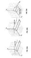
- FIGS. 23 a - 23 c show how three probability functions used to compute FOMs correspond to shapes in bit category index space enclosing tolerated counts of to memory array bits in various categories for the No Repair at Test case, according to one embodiment of the invention.
- FIGS. 24 a - 24 b show the bit category index space volumes enclosing tolerated bit counts in various categories corresponding to Overkill (Mfg) and EUFF for the No Repair at Test case of a memory array, according to one embodiment of the invention.
- FIGS. 25 a - 25 c show the Passes Test ( FIG. 25 a ) and Good in Use ( FIG. 25 b ) categories represented as volumes in bit category index space, and the intersection of these categories ( FIG. 25 c ), for a memory array in the Repair at Test case, according to one embodiment of the invention.
- FIG. 26 shows an example user interface of an Excel calculator, which implements the models in this invention.
- FIGS. 27-28 show graphs of figures of merit vs. test retention time setting, with ( FIG. 27 ), and without ( FIG. 28 ), fault tolerance according to one embodiment of the invention.
- FIGS. 29 a - 29 c show, for the case of no fault tolerance, graphs of figures of merit for test coverage models different from the conservative test coverage model ( FIGS. 29 a and 29 b ), and for the case of perfect correlation between test and use ( FIG. 29 c ), according to one embodiment of the invention.
- FIGS. 30 a - 30 b compare a case for which Test tolerates, but does not repair, up to two failing bits with a case for which Test tolerates and repairs up to two failing bits, according to one embodiment of the invention.
- FIG. 31 is a graph showing that if Test tolerates and repairs up to two failing bits, and arrays in Use can tolerate one failing bit, compared to FIG. 30 b , in which Use tolerates no failing bits, the EUFF is improved (reduced), and Overkill becomes the main component of Yield Loss, according to one embodiment of the invention.
- FIG. 32 a shows a flow diagram of the Model Extraction part of the statistical methodology in which Monte-Carlo synthesis generates Data Replicates, according to one embodiment of the invention.
- FIG. 32 b shows a flow diagram of the Model Extraction part of the statistical methodology in which resampling of the data using the Bootstrap method generates Data Replicates, according to one embodiment of the invention.
- FIG. 33 shows a flow diagram of the Inference part of the statistical methodology, according to one embodiment of the invention.
- FIG. 34 shows a schematic graph of the method for setting guard bands to account for sampling variation due to the Experimental Design and Parameter Extraction parts of the Model Extraction method, according to one embodiment of the invention.
- FIGS. 35 a - 35 b show geometrical constructions on the stripe pseudo-copula to derive a Monte-Carlo sampling algorithm for a censored sub-population of the stripe copula, according to one embodiment of the invention.
- FIG. 36 shows basis vectors for sampling the area of uniform probability in the wedge pseudo-copula, A(u, v), according to one embodiment of the invention.
- FIG. 37 shows the integration limits for an integral used to derive an expression for the subpopulation Kendall's tau of the wedge geometrical copula, according to one embodiment of the invention.
- test chip for the integrated circuit (IC) case would be replaced by “prototype system” (or similar) for the system case; “module” (or “bit” for the DRAM example) for the IC case would be replaced by “component” for the system case, and so on.
- the method includes acquisition of data from a test vehicle, where the test vehicle can be a test chip or product different from the product for which specifications are being determined. Differences between the product and the test vehicle may include different test specifications, datasheet specifications, and different design specifications. Examples of design specifications include the number (e.g. array size) of modules (e.g. bits) and the degree and type of fault tolerance required.
- the method further includes fitting the test vehicle data to a statistical model using an appropriately programmed computer, and using the statistical model to compute figures of merit using the appropriately programmed computer. Since the data acquired using a test vehicle includes measurements of dependent (e.g. correlated) attributes, it is necessary for the statistical model to describe this dependency. The method uses a copula-based statistical model to comprehend the dependency.
- the copula-based model is used to compute figures of merit and compare them with target values to determine specifications that meet requirements of the integrated circuit product. Because of properties unique to copulas, such as the decoupling of marginal distributions from the core dependency structure, the copula-based statistical model gives significant advantages in model fitting and in making inferences.
- the following algorithms and equations of the current invention are implemented in a software tool using a computer, which allows the user to specify attributes of the product such as number of modules (e.g. array size), fault tolerance characteristics, manufacturing test set points and limits, and datasheet specifications of the product.
- the tool outputs values of figures of merit such as yield loss, overkill, and end-use fail fraction.
- the algorithms can also be implemented as plug-in software modules in larger software programs such as optimization engines.
- the copula can be characterized independently of marginal distributions. For example, empirical rank statistics such as Kendall's tau provide a view into the underlying dependency structure (the copula), without interference by details of marginal distributions. Further, it is likely that a population copula that is independent of environmental conditions may be found since it contains only rank statistical information, which is relatively undisturbed by environmentally-induced changing marginal distributions. If an environmentally independent copula can be found, a great simplification of the model obtains, and advantages such as “equivalent set points”, explained below may be realized. Additionally, copula models have an advantage over the prior art because different copula models may be tried without changing any other part of the analysis, whereas for multi-normal models the marginal and dependency structures are entangled.
- Copula-based methods have a much greater flexibility than the multi-normal-based methods usually employed to represent the dependency structure of parametric attributes.
- Multi-normal statistics are a special case of the Gaussian copula described in this invention, and share the shortcomings of the Gaussian copula.
- a key shortcoming of the Gaussian copula, and therefore of the usual multi-normal model, is that these models cannot properly represent correlation that extends deep into the tail of multi-variate distributions, whereas, according to the current invention, many copulas can do this.
- the DRAM example below requires a deep-tail-dependence copula, which will be shown not to be satisfactorily modeled using the Gaussian copula.
- each memory bit of a dynamic random access memory retains its information as stored charge on a capacitor. After the bit has been written to, the charge leaks away so that valid data has a characteristic retention time. To retain the information, the bit must be read and refreshed.
- DRAM memory cells can have a defect, which causes a few bits to have a variable retention time (VRT), while most bits have stable retention times (SRT).
- VRT variable retention time
- SRT stable retention times
- the VRT behavior is caused by a silicon lattice vacancy-oxygen complex defect when the defect is embedded in the near surface drain-gate boundary of a DRAM cell.
- the defect can transition reversibly between two states. One of the states is associated with a leaky capacitor and short retention times.
- the VRT mechanism causes a soft-error reliability issue in DRAM arrays since a VRT bit may be tested and pass a brief retention time screen while in the low leakage state, but in extended use, a high leakage state will almost certainly occur possibly with retention time less than the system-specified refresh time.
- This miscorrelation of retention time between test and use is perceived as a soft-error reliability issue, which requires error correction methods to make the DRAM tolerant of single bit errors.
- This example of the invention shows how to measure and model this miscorrelation in a DRAM case study to establish test specifications such as set points (temperature, voltage) and limits (retention time), establish datasheet specifications (temperature, voltage, refresh time), and determine sufficient levels of fault tolerance to meet quality and reliability requirements.
- Test chips with four identical DRAM arrays on each chip were fabricated in five skews of a 65 nm process as shown in Table 1. Each of the four arrays on a chip has 1218750 bits. The test chips were packaged in ball grid array packages and 10 randomly selected test chips from each of the process skews were selected for this example.
- the arrays were tested on a Credence Pair tester with 145 I/Os and seven power supplies and the temperature was controlled by a Silicon Thermal Powercool LB300-i controller. Retention time for each bit was measured at 18 environmental conditions:
- the pattern ( FIG. 1 ) of retention time failures observed for each bit was used to classify a bit as not failing (r>604 au), or as failing by either variable retention time (VRT) or by stable retention time (SRT). If a bit failed on the first reading on any loop, it was also classified as a zero retention time ZRT bit. At each environmental condition any given failing bit may be classified as SRT or VRT and ZRT or not-ZRT. The classification of a given bit may be different in a different environmental condition.
- SRT r index varies by ⁇ 1 within loop, or loop-to-loop (two examples).
- VRT r index varies by ⁇ 2 within loop, or loop-to-loop (two examples).
- r index 0 in any loop. r index varies by ⁇ 1 within loop, or loop-to-loop (two examples).
- the pass/fail patterns were processed to extract the index of the smallest passing retention time, i min , and the index of the longest passing retention time, i max , i max was found by “AND-ing” all loops for a bit and finding the index of the first “0” counting from the right.
- SRT stable retention time
- the margin of 1 allows for the possibility of tester variation in case the bit retention time falls on a retention time bin boundary.
- FIG. 3 shows data for a few failures (rows) copied from the Excel workbook containing all the data.
- the field names (columns) are defined in Table 2.
- IRetDelta IRetMax-IRetMin If IRetMin > 0 and IRetDelta ⁇ 1, the bit is a SRT bit. If IRetMin > 0 and IRetDelta > 1, the bit is a VRT bit Loop Groups Pass/Fail record of bit at specified environmental condition.
- the method of this patent requires extraction of a statistical model for the actual retention times for each bit, rather than of the coarse categories (SRT, etc.) into which bits may fall according to their retention time behavior.
- every failing bit will have minimum retention time of r min and a maximum retention time of r max observed in the course of 60 repeated measurements (12 measurements in five loops).
- the retention time of a bit at Test, r test is measured just once, and the retention time in Use, r use , is sampled an indefinitely large number of times as the memory is used.
- the next step is to extract empirical marginal distributions for Test and Use by summing fail counts in rows, and in columns, and then computing the cumulative fail count and cumulative fraction fail for each. This was done for each of the 5 skews at each of the 18 environmental conditions.
- the marginal distributions of Test and Use for the DRAM are the same, apart from some sampling noise, because of the symmetrical way in which r min , and r max were assigned to r use and r test . Notice from the figure that only a tiny part of the entire sample space near the origin is of practical significance—a fraction of only about 34 parts per million (PPM) of the sample space was observed. This is typical of integrated circuit test correlation data.
- FIG. 7 is a plot of ln( ⁇ ln(1 ⁇ F)), known as the “Weibit”, versus ln(r). Slope and intercept of lines fitted to these data give estimates of the shape, ⁇ , and scale, ⁇ , parameters of the Weibull distribution of retention time, r, in
- this method extracts a value of the natural log of the characteristic retention time, ln ⁇ , for each of 18 environmental conditions.
- the characteristic retention time, ⁇ accurately fits an exponential voltage dependence and Arrhenius temperature dependence:
- ln ⁇ ⁇ ⁇ ln ⁇ ⁇ ⁇ 0 + a ⁇ ( V p - V p ⁇ ⁇ 0 ) + b ⁇ ( V d - V d ⁇ ⁇ 0 ) + Q k B ⁇ ( 1 T - 1 T 0 ) ( 2 )
- the subscript 0 indicates a reference environmental condition.
- the reference condition has been chosen arbitrarily as the maximum stress condition in the experiment.
- ln ⁇ 0 is the natural logarithm of the characteristic retention time in au at this condition.
- V d is the supply voltage
- V p is the substrate bias voltage
- T (° K) is the temperature. The quality of the fit is shown in FIG. 8 .
- the activation energy of retention time is between 0.6 eV and 1 eV for SRT bits and VRT bits in the low-leakage state and about 0.2 eV for VRT bits in the high leakage state.
- the fitted value of Q is about 0.6 eV (Table 4). This is expected since most observed bits are in the low leakage state.
- the low activation energy of VRT bits in the high leakage state could lead to under-estimates of customer risk if the model is extrapolated beyond the range of the data on the low temperature side. However, the data spanned the test conditions and use conditions so extrapolation is not needed.
- Kendall's tau is a statistic used in the invention to measure the similarity of the rank orderings between a pair of attributes measured on a population of units. Its value ranges from 1 when the ranks are the same, through 0 when there is no relationship between ranks, to ⁇ 1 when the ranks are opposite.
- ⁇ (x 1 , y 1 ), (x 2 , y 2 ), . . . (x n , y n ) ⁇ denotes a random sample of n observations sampled from a population 2-vector of continuous random variables, (X, Y).
- Any pair of observations, i and j may be labeled “concordant”, or “discordant”, according to whether the sense of the inequality between x i and x j is the same or the opposite to the inequality between y i and y j .
- Kendall's tau for the random sample is defined as
- Test data such as FIG. 6
- the sample tau for data with ties is
- ⁇ ′ c - d 1 2 ⁇ n ⁇ ( n - 1 ) - U ⁇ 1 2 ⁇ n ⁇ ( n - 1 ) - V ( 4 ) where now any pairs that are tied in x or y are not counted in either c or d, and where
- Eq. (5) is over all sets of tied x-values, and u is the number of tied x values in each set. V is defined in the same way, but for y-values. Code to implement (4) is known.
- Eq. (4) was used to compute Kendall's tau for the measured sample of retention time data. These values are plotted as a function of environmental condition for the nominal skew in FIG. 9 , along with the fraction of the population of 48750000 bits tested. Note that the sample tau is independent of environmental condition (ln ⁇ ) and the degree of censoring (sample fraction). This was true for all skews, not only the nominal skew shown in FIG. 9 . Moreover, since Table 4 shows the average value of tau across environmental conditions for each skew, it is clear that the value of tau does not vary greatly from skew to skew. This key result is consistent with an environmental and skew independence of the underlying dependency structure of the DRAM VRT behavior embodied in the copula.
- FIG. 6 is an empirical sampling of a bi-variate probability density function (pdf), which here is taken to be h(x, y).
- PDF bi-variate probability density function
- r use / ⁇ is denoted by x
- r test / ⁇ is denoted by y.
- the off-diagonal cells in FIG. 6 are populated by counts of units for which Use and Test measurements of retention time are miscorrelated.
- the marginal cumulative distributions for Test and for Use are also shown in FIG. 6 by the dashed-line areas. Separation of modeling of marginal distributions from modeling the dependency structure of the data is a key aspect and major benefit of the current invention.
- FIG. 10 A geometrical interpretation of Eq. (8) is shown in FIG. 10 , where for perfect correlation, the probability density is a delta function on the diagonal.
- the two-dimensional cdf is the probability mass enclosed by a rectangle with one corner pinned at (0, 0).
- Copulas have four defining properties.
- a 2-dimensional copula is a cdf with range [0, 1] on domain [0, 1] 2 (the unit square) which has the following properties:
- Eq. (18) The expression on the left side of Eq. (18) is the probability mass in the region defined by u 1 , u 2 , v 1 , v 2 in [0, 1] such that u 1 ⁇ u 2 and v 1 ⁇ v 2 .
- the method of computing probability mass in a sub-area of [0, 1] 2 shown in FIG. 11 is used extensively in the description of this invention.
- a pseudo-copula relaxes condition 3, Eq. (17).
- a copula is fitted to test vehicle data, and then a pseudo-copula is constructed to make model inferences.
- a pseudo-copula is also the starting point for definition of a class of “geometrical” copulas described in this invention.
- a 2-dimensional copula is the fraction of the population failing by both marginal cdfs (that is, u ⁇ 1 and v ⁇ 1) as a function of the marginal fail cdfs, u and v.
- the foundation of the copula method is Sklar's theorem, which states that the decomposition of a given multidimensional cdf H into its marginal distributions and the function C in Eq. (12) is unique. That is, there is only one function C, which satisfies Eq. (12) for a given H. Moreover, it has been shown that the copula corresponding to a joint cdf of statistical variables is invariant under strictly increasing transformations, say ⁇ and ⁇ , of the arguments of the cdf.
- a copula contains all the information of rank dependency of its marginal variables.
- Kendall's tau is a statistic which summarizes this rank dependency. Tau is best understood by considering how to compute the “sample” tau from data (real or synthesized) per Eq. (3). Less intuitively, the “population” tau can also be computed from the analytical form of a copula using the known formula:
- tau does not in general uniquely determine the copula, for a family of copulas spanned by a single parameter, a sample estimate of tau from data can be used to determine the parameter.
- the parameter of the copula is determined by adjusting it to make the model population value of tau from Eq. (23) match the sample estimate of tau. This gives an easy way to fit single-parameter copula models to data provided that the data is sampled from the entire population space. However, test data is typically highly censored. Remember that the conditions of the DRAM experiment span only about 40 PPM near the origin of the copula.
- the sample tau for the censored data can still be used to determine the copula parameter if the model tau is computed only from part of the population model copula corresponding to the censored data. If Test and Use right-censor x and y x i ⁇ a,y i ⁇ b (24) then the “sub-population” model tau computed from a generalization of Eq. (23) for a restricted domain, [0, u a ⁇ F(a)] ⁇ [0, v b ⁇ G(b)] of [0, 1] 2 is
- ⁇ subpopulation 4 C 2 ⁇ ( u a , v b ) ⁇ ⁇ 0 u a ⁇ d u ⁇ ⁇ 0 v b ⁇ d vC ⁇ ( u , v ) ⁇ ⁇ 2 ⁇ C ⁇ ( u , v ) ⁇ u ⁇ ⁇ v - 1 ( 25 ) which depends on the censor limits a and b, as well as the parameter(s) of the copula.
- Eq. (25) is a new result, derived below, which is part of the invention described here.
- an alternative method of computing tau is Monte-Carlo (MC) synthesis of data from a copula by any of many known methods, and evaluation of tau using Eq. (3). This is a good way to evaluate the population tau corresponding to Eq. (23). But the MC evaluation of the copula model subpopulation tau corresponding to the highly censored data can be very inefficient if the samples cannot be confined to the region of the data, and many samples must be rejected.
- a geometrical copula of the kind described in this invention provides a way to compute the subpopulation tau by the MC method with complete efficiency because samples can be confined to any sub domain of the copula. This is not true of copulas in general.
- copula makes sense for the particular application.
- many sometimes exotic functions that are copulas.
- Archimedian copulas have nice algebraic properties, which Make them tractable and model-fitting methods have been developed, but it is often hard to relate them to a plausible underlying mechanism, and even to appreciate their geometrical shapes.
- a non-Archimedian example is the Marshall-Olkin copula, which is a natural bi-variate extension of the Poisson process and so has an intuitive stochastic interpretation.
- a third example is the Gaussian copula, which is a well-known extension of the multi-normal distribution. As shown below, when the Gaussian copula is fitted to the data of the DRAM example it had the drawback that its parameter was forced to an implausible limit to fit the data.
- Geometrical copulas offer an intuitive and practical approach to the problem of choosing a copula for manufacturing test applications.
- Geometrical copulas define probability densities along easy to visualize lines and regions of the copula's domain. These shapes can be adjusted by parameters with geometrical interpretations.
- test data is acquired over a range of environmental conditions and sample sizes, which span the application over which the model is used. This means that the copula needs to “look like” the data, and the fitted model will not be used to extrapolate far from the data.
- the “stripe” and the “wedge”, in addition to the Gaussian copula are derived and fitted to the data.
- copula models provide a deterministic semi-analytical way to compute figures of merit used to characterize, and so specify, the test manufacturing process. This is much more efficient than doing a Monte-Carlo (MC) synthesis from the models. But sometimes, MC synthesis is unavoidable, and the current invention provides MC synthesis in these cases.
- Another major benefit of geometrical copulas (not shared with the Gaussian copula, for example) is that it is possible to generate MC samples only in the important tail region, without wasting samples in the larger domain of the copula. This will be shown for the geometrical copulas described below.
- a method of modeling dependence is to treat variables as multi-normally distributed correlated statistical variables.
- the cdf is
- the correlation coefficient, ⁇ 1 ⁇ 1, quantifies the dependence.
- the Gaussian copula is commonly used, it will be fitted to the DRAM data as an example which will make clear the benefits of the new geometrical-copula-based method described in this invention.
- the related t-copula has a finite value of LT, and so may be more suitable than the Gaussian copula, but it shares the other advantages and, particularly the disadvantages, of the Gaussian copula for the test applications described in this invention.
- the data in FIG. 6 is concentrated along a diagonal, with some scatter to either side. This suggests using a copula in which has finite probability density in a diagonal stripe on either side of the diagonal, but vanishing probability density outside the stripe.
- the width of the stripe can then be adjusted by a parameter. Both the shape of the stripe and the probability density are adjusted to make the margins uniform so that it is a copula.
- the stripe copula is constructed by first drawing a diagonal stripe across the unit square shown in FIG. 13 to construct a stripe pseudo-copula.
- the parameter d controls the width of the stripe, which can range from zero (perfect correlation), to covering the entire unit square uniformly (independence).
- the probability density in the stripe is uniform, normalized to unity, and vanishes outside the stripe.
- the uniform probability density of the stripe in FIG. 13 is 1/(2d ⁇ d 2 ), the reciprocal of the stripe's area.
- A(u, v) is the function which gives the probability enclosed by the rectangle (0, 0)/(u, v).
- expressions for the probability density A(u, v) enclosed by the boundaries of the rectangle (0, 0)/(u, v) shown in FIG. 13 may be found as a function of (u, v). All of these cases are covered by the formula for the stripe pseudo-copula
- the function A is a pseudo-copula because it satisfies the requirements of a copula except that the margins are not uniform.
- z is a dummy argument which can be either u, or v.
- the function ⁇ ⁇ 1 (z) is:
- Algorithms for Monte-Carlo synthesis of random points in geometrical copulas such as the stripe copula can be derived using geometrical arguments starting with the pseudo copula, A. It is possible to fill any parallelogram or triangle with uniformly distributed random points using every point generated, that is, without the rejection of any Monte-Carlo sample. This is done by weighting the basis vectors that define the parallelogram with a pair of independent uniformly distributed random numbers. For a triangle, points in the “wrong half” of a parallelogram are reflected into the triangle of interest. The slice in FIG. 13 can be decomposed into rectangles and triangles, and random points placed in them according to probabilities determined by area ratios of the rectangles and triangles.
- FIGS. 14 a - 14 f show examples of synthesized probability maps of the stripe copula.
- the density of random points indicates the probability density of the copula. Notice that both the shape and the density of points have been transformed by the function ⁇ , Eqs. (33) and (34), from the pseudo-copula of FIG. 13 .
- the degree of censoring, or censor fraction is indicated in FIGS. 14 a - f by the parameter “Censor”.
- the censor fraction is the number of units in a sample or sub-population divided by the number of units in the entire population.
- Kendall's tau is computed from the synthesized data using Eq. (3) and is also shown in the header of plots in FIGS. 14 a - f . Recall from Table 3 that DRAM bits for which retention times were measured covered only 40 PPM of the population. This degree of censoring, typical of integrated circuit test applications, would be a tiny dot near the origin on the scale of the plots in FIGS. 14 a - f .
- the data in FIG. 6 appears to be more scattered as retention time increases.
- the construction starts with a wedge-shaped pseudo-copula A(u, v) symmetrical about the (0, 0)/(1, 1) diagonal with uniform probability density inside the wedge, and vanishing probability density outside the wedge, shown in FIG. 15 .
- This shaded region has area (1 ⁇ c)/c, where c is defined in the figure, so the wedge's uniform probability density is c/(1 ⁇ c).
- the wedge pseudo-copula can be shown by geometrical considerations to be the probability density enclosed by the (0, 0)/(u, v) rectangle in FIG. 15 for (u, v) anywhere in [0, 1] 2
- ( 42 ) f - 1 ⁇ ( z ) ⁇ ( c + 1 ) ⁇ z 2 2 0 ⁇ z ⁇ c - 1 z - ( 1 - z ) 2 2 ⁇ ( c - 1 ) c - 1 ⁇ z ⁇ 1 ( 43 ) which is a monotonically increasing function of the dummy argument, z.
- A(u, v) is a pseudo-copula because the marginal distributions, Eqs. (42), are not uniform.
- Eqs. (43) is needed:
- f ⁇ ( z ) ⁇ 2 ⁇ z c + 1 0 ⁇ z ⁇ 1 + c 2 ⁇ c 2 c - ( c - 1 ) 2 + 2 ⁇ ( c - 1 ) ⁇ ( 1 - z ) 1 + c 2 ⁇ c 2 ⁇ z ⁇ 1 ( 44 )
- the algorithm for generating (u, v) points is given below.
- the probability density maps of the wedge copula in FIGS. 16 a - 16 f were generated using this method. Notice that it is possible to restrict the generation of synthesized points to sub-domains of the copula, particularly the region near the origin.
- FIGS. 16 d - 16 f show that synthesized points can be concentrated near the origin, corresponding to values of the censor fraction, “Censor” ⁇ 1.
- the wedge copula has the attractive property that the subpopulation tau is independent of a, the censor fraction. This is not true of copulas in general as may be seen by comparing the cases in FIGS. 14 a - 14 f and FIGS. 16 a - 16 f for which the parameter d or c, respectively, is constant, but the censor fraction varies. Since tau may be computed directly from data, Eq. (53) provides a way to estimate the parameter c of the wedge copula, according to the current invention.
- the dependent attributes of a test vehicle or product are expected to be related only by the intrinsic physics of the materials and design, and defects will affect one or the other but not both of the attributes, then one can expect that dependency will be strong in the bulk but weak in the tails of the two-dimensional distribution.
- a least-squares method was used to extract the best fit copula at each of the 18 environmental conditions for each skew of the DRAM data. The following sum was minimized using Excel's solver to determine p, and the copula-specific model parameter:
- a simpler and more convenient way than the least-squares method to extract the parameter of the copula is to compute a “sample” estimate of Kendall's tau directly from the data and compare it with the theoretical expression for the subpopulation tau, Eq. (25), to solve for the parameter.
- the theoretical expression for the subpopulation tau is generally also a function of the censor fraction, which is known from the experiment.
- an estimate of c may be derived by substituting the sample tau computed from the data using Eq. (3), and given in Table 4, into the inverse of Eq. (53), written as
- FIG. 17 a shows estimates of c as a function of the 18 environmental conditions, ln ⁇ . Estimates using Eq. (57) and the more generally applicable least-squares method show good agreement in the figure. Moreover, the figure shows that c is independent of the environmental condition.
- FIG. 17 b shows a reasonably environmental-condition-independent fit to the Gaussian copula by the least-squares method. It was not possible to determine the copula parameter using the sample tau method because there is no easily derived expression from Eq. (25), nor is it possible to do an efficient Monte-Carlo computation of the sample tau because there is no known way to confine random samples to the tail of the copula without rejection of points.
- the range of the data covers only 40 PPM of the population (for the nominal skew), so sampling the entire population to estimate tau for the range of the data is not practical.
- the best least-squares fit was obtained for a correlation coefficient of about 0.999 (see FIG.
- FIG. 17 c shows parameter estimates for the stripe copula as a function of environmental condition, ln ⁇ , for both the least-squares and the sample tau methods.
- FIG. 18 shows a comparison of minimum sums of squares computed from Eq. (55) for each of 18 environmental conditions for the nominal skew. Most of the plotted points in FIG. 18 are above the diagonal, showing that the wedge copula gives the best fit.
- the wedge copula model was selected to model the dependency structure of the DRAM bit retention time.
- FIG. 20 shows how good and bad (defective) units of an integrated circuit product such as a memory array are produced by the Fab/Assembly process, and then are screened by final Test and go on to Use.
- the figure also shows important figures of merit (FOMs) including Yield Loss, Overkill (there are two kinds), and End-Use Fail Fraction.
- FOMs figures of merit
- FIG. 21 a schematic drawing of how the Test and Use conditions divide the population of manufactured units into categories is shown in FIG. 21 .
- the three proportions shown in FIG. 21 which are modeled as probabilities, are sufficient to characterize the effect of Test and Use.
- the four FOMs described next are defined in terms of these probabilities.
- EUFF ⁇ P ⁇ ( Fails ⁇ ⁇ in ⁇ ⁇ Use
- Passes ⁇ ⁇ Test ) ⁇ 1 - P ⁇ ( Good ⁇ ⁇ in ⁇ ⁇ Use
- Passes ⁇ ⁇ Test ) ⁇ 1 - P ⁇ ( Passes ⁇ ⁇ Test ⁇ ⁇ and ⁇ ⁇ Good ⁇ ⁇ in ⁇ ⁇ Use )
- P ⁇ ( Passes ⁇ ⁇ Test ) ⁇ P ⁇ ( Passes ⁇ ⁇ Test ) - P ⁇ ( Passes ⁇ ⁇ Test ⁇ ⁇ and ⁇ ⁇ Good ⁇ ⁇ in ⁇ ⁇ Use ) P ⁇ ( Passes ⁇ ⁇ Test ) .
- EUFF is the fraction of units classified as failing in Use, given that they have passed Test (a conditional probability).
- End-Use Fail Fraction (EUFF) is a primary quality indicator since it is the customer-perceived proportion of defective units.
- each FOM is a ratio falling into the range [0, 1] and that for each, “0” is most desirable and “1” is least desirable. So specifications for a product and test manufacturing process are found by requiring that FOMs meet do-not-exceed targets for each FOM. Targets are chosen with producer costs and customer-perception of brand image in mind, and are product-specific. Quality-related customer costs are one aspect of this perception.
- one embodiment of the invention specifies these in terms of environmental conditions (V p , V d , T) and retention time, r.
- the settings of these four parameters in Use (Datasheet Specification) and at Test (Test Condition) will be different. Usually the Test Condition is more “stressful” than the Datasheet Specification.
- the environmental condition is mapped into the single parameter ⁇ use in Use and ⁇ test in Test.
- the datasheet specifies a refresh time r use , and the Test specification uses a different retention time limit setting, r test . So, a single parameter, x, depending on both the environmental condition via ⁇ and retention time limit r use in the datasheet defines the Datasheet Specification (Use) condition:
- Figures of merit are used in cost models of the integrated circuit product. Costs to the producer of a component and costs to the customer producing systems using the component must be included in these models. Regarding producer costs, suppose the cost of manufacturing a component is $Cost and the sale price of a component is $Price, and suppose N component units are to be manufactured. Besides costs of materials used in the unit, $Cost includes per-unit capital depreciation costs associated with the manufacturing equipment such as testers, charged to the unit. For testers, this cost-contributor will depend on the time needed to test each unit, among other factors.
- overkill may significantly affect the business viability of a product.
- EUFF Error Correction Factor
- the cost impact of a defective component to a system manufacturer is usually much greater than the price of the component, particularly for surface-mounted components. Therefore, EUFF is typically required to be less than about 200 DPPM. Beyond cost, EUFF has a qualitative impact on brand image. This is often the primary consideration in choosing the EUFF target.
- test coverage model For the copula-based statistical model fitted to the data, the test coverage model used assumed that the minimum and maximum retention times for each bit are equally likely to occur in Test and in Use. This is called a “symmetrical test coverage model”. However, for a realistic Manufacture/Test/Use flow like FIG. 20 , Use occurs over extended time periods, so that if a minimum retention time can occur for a bit it will certainly occur in Use. On the other hand, Test is brief so the probability of occurrence of the minimum or the maximum retention time of a bit in Test depends on details of time-in-state of bit-leakage which are beyond what can be known from the DRAM example data.
- test coverage model The most conservative assumption from the end-user perspective, called the “conservative test coverage model”, is that Use always “sees” the minimum retention time and that Test always “sees” the maximum retention time. Other test coverage model assumptions are also used to model Test and Use in order to gauge the sensitivity of the model to this assumption.
- r test is the 2:2 order statistic
- r use is the 1:2 order statistic of the pair (r′ test , r′ use ). It is known that the 2-dimensional cdf connecting the 2:2, and 1:2 order statistics of a pair of random variables distributed according to a 2-dimensional cdf H(u, v) is
- So D is the transformation of the fitted copula, C, embodying the conservative test coverage model that Test always “sees” r max and Use always “sees” r min .
- An integrated circuit DRAM memory includes an array of many, N, bits.
- the preceding description gives a model of the dependence structure, D, of retention times for a single bit. Needed is a model of the dependence structure of retention times for an N-bit array.
- N-bit arrays which are good only when all N bits are good.
- the more realistic and complex cases when an array can be good if some bits are bad (fault tolerance) and when arrays with bad bits can be repaired at Test will be described later.
- Eq. (73) and (74) can be generalized in an obvious way to get the survival copula of a product with multiple copies of several types of module for which copula models were extracted from test vehicle data. (For the DRAM, there is one type of module; the bit.) In particular, Eq. (73) becomes a product over module types with the survival copula of each module raised to a power which is the number of modules of that type in the product.
- FIG. 22 shows a schematic representation of how the Test and Use conditions in Eqs. (62) and (63) superimposed over the bit pseudo-copula pdf of Eq. (71) divide the population probability space into four regions labeled according to a bit's Use/Test pass/fail category.
- This depiction is schematic because, for the DRAM, x and y are much closer to the origin than shown.
- FOMs can be expressed in terms of the probability mass (shaded) enclosed in each of the four labeled regions of the population probability space, and the probability masses can be expressed in terms of the pseudo-copula D.
- the essential tradeoff between overkill and end use fraction fail can be seen in FIG.
- Eq. (83) shows that for perfect correlation, EUFF vanishes if the Test condition exceeds the Use condition, and it quantifies the fraction failing whenever the test condition is made less than the use condition.
- the behavior of the overkill FOMs complement this, showing the essential tradeoff between EUFF and overkill. Notice that Use and Test conditions are quantified by the single parameter r/ ⁇ and ⁇ depends on V p , V d , and temperature.
- the array model is generalized to take account of fault tolerance at Test and in Use.
- fault tolerance is implemented by physically remapping of failed bits to a small number of rows or columns
- ECC error correction redundancy coding
- Statistical models of the effect of fault tolerance schemes on FOMs is done by expanding the definition of a “good” array to include arrays with some “bad” bits. “Bad” bits in arrays that are considered “good” are taken to be covered by a fault tolerance scheme. The maximum number of “bad” bits that can be tolerated is a measure of the repair capacity of the fault tolerance scheme. Only the repair capacity of a fault tolerance scheme is needed to estimate the effect on FOMs.
- the expressions for FOMs for two fault tolerant cases are derived.
- the cases are 1) No Repair at Test, and 2), Repair at Test. In the first of these cases the tester does not actively repair any failing bits that it finds, whereas in the second case the tester can repair some failing bits.
- FOMs depend, in turn, on these probabilities via Eqs. (58), (59), (60), and (61).
- the Poisson limit is well-justified for the DRAM since typical arrays have many thousands of bits with only tens of failing bits at most. Moreover, the mathematical manipulations are more tractable in this limit.
- Fault tolerance schemes in Test and in Use may be described by a set of constraints on the range of indices over which the sums of terms like Eq. (86) range in expressions for the probability functions appearing in the expressions for the FOMs, Eqs.(58), (59), (60), and (61).
- sets of allowed values of n ff , n pf , and n fp consistent with the constraints may be computed once for any test and array design scheme and then be reused to compute FOMs for different values of ⁇ ff , ⁇ pf , and ⁇ fp .
- attention is confined to cases for which FOMs may be computed even more conveniently using special functions. Two cases will be considered: No Repair at Test, and Repair at Test.
- n is a measure of the transparency of Test to failing bits.
- the Repair at Test case would restore up to n t failing bits to functionality by, for example, replacing a word with a bad bit with a word with all good bits.
- n t is a measure of the size of the supply of spares.
- n u and n t are usually small integers, which makes evaluation of various required functions easy.
- PT_NR ⁇ n ff , n pf , n fp ⁇ : 0 ⁇ n ff + n pf ⁇ n t 0 ⁇ n fp ⁇ ⁇ ⁇ ( 88 ) which leads to
- P ⁇ ( Passes ⁇ ⁇ Test ) ⁇ PT_R ⁇ ⁇ ⁇ ff n ff ⁇ e - ⁇ ff n ff ! ⁇ ⁇ fp n fp ⁇ e - ⁇ fp n fp ! ⁇ ⁇ pf n pf ⁇ e - ⁇ pf n pf !
- the second probability function required for the No Repair at Test case is the Good in Use probability function where an array is defined as good in use with up to n u bits failing.
- the permitted counts of bit categories for arrays in the Good in Use (irrespective of Test) category is the set of integers:
- the third probability function required for the No Repair at Test case is the Passes Test and Good in Use probability function.
- the permitted counts of bit categories for arrays in the Passes Test and Good in Use category is the set of integers
- the set of integers PTGIU_NR is the intersection of the sets PT_NR and GIU_NR.
- the function K shown in Eq. (146) below, is easy to evaluate because it is a sum of a small finite number of terms involving products of the function R.
- the Passes Test and Good in Use category is the intersection of these prisms. For no fault tolerance, the allowed integers collapse to the single point at the origin, (0, 0, 0). Because the three probability functions used to compute FOMs correspond to shapes in index space shown in FIGS. 23 a - 23 c , the FOMs derived from these probability functions via Eqs. (58), (59), (60), and (61) also correspond to volumes in index space. The volume corresponding to Yield Loss is the entire space outside the prism in FIG. 23 a . The volumes for Overkill (Mfg) and EUFF [apart from the normalizing factor, P(Passes Test)] are shown in FIGS. 24 a - 24 b .
- the Passes Test probability function for the Repair at Test case is defined by the same set of integers as the No-Repair at Test case because the criterion for rejecting an array at Test depends only on the number of bits tolerated at Test, not on whether or not any of the tolerated bits are repaired. So the Passes Test category of arrays in the Repair at Test case is defined by the set of integers:
- the effective number of ff and pf bits affecting the post-test classification of the array is the union of the ff and pf categories, minus n t : n ff +n pf ⁇ n t . If it is assumed that the repair process does not distinguish between ff and pf bits (both kinds are detected as fails in Test), then the proportion of ff and pf bits affecting post test array classification is the same as the pre-test proportions of these bit categories. So one may model the post-test ff bit count, which must figure into classification of arrays in Use as
- GIU_R ⁇ n ff , n pf , n fp : 0 ⁇ n ff ′ ⁇ ( n ff , n pf , n t ) + n fp ⁇ n u 0 ⁇ n pf ⁇ ⁇ ⁇ ( 98 )
- n ff n′ ff ( n ff ,n pf ,n t ) for n pf ⁇ m.
- the set of integers GIU_NR is a subset of GIU_R. That is
- GIU_R GIU_NR ⁇ ⁇ ⁇ ⁇ GIU_R ⁇ ⁇
- GIU_R GIU_NR ⁇ ⁇ ⁇ ⁇ GIU_R ⁇ ⁇
- ⁇ GIU_R ⁇ n ff , n pf , n fp : 0 ⁇ n ff ′ ⁇ ( n ff , n pf , n t ) + n fp ⁇ n u n ff + n fp > n u 0 ⁇ n pf ⁇ m ⁇ ( n u , n t ) - 1 ⁇ ( 102 )
- Eq. (102) the second inequality ensures that the integers in ⁇ GIU_R are not in GIU_NR, and the final condition limits the range of n pf to cases where n ff ⁇ n′ ff is possible, for the purpose of efficiency.
- a geometrical interpretation of GIU_R is shown in FIG. 25 b . Notice that, in FIG. 25 b , ⁇ GIU_R is represented by the 5-sided polyhedron atop the Good-in-Use prism for GIU_NR shown in FIG. 23 b .
- the sum over the integers GIU_NR has been given by Eq. (92), to which must be added terms resulting from Eq. (102)
- the Passes Test and Good in Use probability function of the Repair at Test case corresponds to the intersection of allowed indexes for the Passes Test and Good in Use cases previously described:
- PTGIU_NR ⁇ n ff , n pf , n fp : 0 ⁇ n ff ′ ⁇ ( n ff , n pf , n t ) + n fp ⁇ n u 0 ⁇ n ff + n pf ⁇ n t ⁇ ( 105 )
- PTGIU_R ⁇ n ff , n pf , n fp : 0 ⁇ n fp ⁇ n u 0 ⁇ n ff + n pf ⁇ n t ⁇ ( 106 ) which has the simple geometrical interpretation shown in FIG. 25 c .
- FIG. 26 The user interface of the calculator is shown in FIG. 26 . Dashed-outlined cells are user inputs, and solid-lined cells are outputs. The main sections of the interface of the Excel calculator tool are described in more detail in the following.
- the Skew, Model Parameters section in FIG. 26 allows the user to select the process skew (Table 1).
- the fitted marginal distribution environmental parameters and wedge copula parameters for the selected skew (Table 3) are displayed.
- An extra skew called “Spare” which is the same as the nominal skew but with a perfect correlation copula, M, is available in addition to the five skews of Table 1 for which parameters were extracted from data.
- the Memory Architecture section in FIG. 26 allows the user to select the array size and number of bits tolerated at Test and at Use.
- the number of bits tolerated at Test is interpreted in two ways: 1) For No Repair at Test, failing bits detected at Test are tolerated but not repaired. 2) For Repair at Test, failing bits detected at Test are tolerated and made good (repaired). A set of FOMs is generated for each way.
- the Test and Use Conditions section in FIG. 26 allows the user to select retention time and environmental conditions (V u , V d , T) for Test and for Use.
- the model also requires specification of the test coverage model, which defines how minimum and maximum retention times for a VRT bits are be distributed between Test and Use.
- the interface provides a choice between the conservative test coverage model in which r max occurs only in Test, and r min occurs only in Use, the aggressive test coverage model for the opposite assumption, and the symmetrical test coverage model for which min/max retention times are equally likely to be in Test or Use.
- FIG. 26 shows the computed four FOMs defined by Eqs. (58), (59), (60) and (61) for the No-Repair-at-Test, and the Repair-at-Test cases.
- FIG. 26 Not shown in FIG. 26 are parts of the interface, which specify targets and plotting limits for the graphs also produced by the calculator.
- the graphs generated by sweeping the Test retention time past the Use refresh time give a good appreciation of the properties of the model. Because environmental conditions enter the model only through ln ⁇ [see Eqs. (62), (63) and (2)], properties of the model may be explored by setting V p , V d , and T to a convenient value (the reference condition in the example shown in FIG. 26 ), and then sweeping the retention time setting in Test past the Use refresh time specification. Plots are generated for which all the input parameters are entered in the user interface as described above, except that the Test retention time (r_t) is swept between the plotting limits defined for it.
- FIGS. 27 , 28 and 29 a - 29 c show how the shape of the FOM characteristics reflect the underlying copula model.
- vertical asymptotes on a logarithmic plot of the Overkill and EUFF figures of merit correspond to the boundaries of the wedge copula, transformed by the test coverage model, at the Use condition. If retention time in Test is always r max and in Use it is always r min , (the conservative test coverage model) as in all figures except FIGS. 29 a and 29 b , then the Overkill vertical asymptote corresponds to the Use condition.
- the case of the symmetrical test coverage model is shown in FIG.
- FIG. 29 a and the aggressive test coverage model is shown in FIG. 29 b .
- FIG. 29 c shows how the case of perfect correlation makes vertical asymptotes of Overkill and EUFF both align with the Use condition.
- Comparison of FIGS. 27 , 29 a , and 29 b gives an example of how the conservative test coverage model maximizes the model estimate of EUFF compared to the symmetrical and aggressive test coverage models.
- the increased Overkill in FIG. 31 is not a “problem”, but is an “opportunity” for some other test method beyond the scope of the manufacturing flow considered here.
- yield loss rejects could be screened by a “Use-like” test to recover (some of) the arrays that are good-in use. Viability of this will be determined by the cost of the additional screening.
- FIGS. 32 a and 32 b show alternative approaches to characterizing sampling variation in the Model Extraction part of the methodology. While, at a high-level, the two-part methodology is prior art, the discussion shows how copula-based statistical models are integrated into the two-part methodology and improve key aspects of it.
- the purpose of the methodology is to determine the design, test manufacturing and datasheet (end use) specification of an electronic system or integrated circuit product, taking into account dependent attributes of the product.
- Model Extraction is a Statistical Model of the test vehicle fitted to the data.
- the Statistical Model is then used by the Inference part of the methodology to compute FOMs for product design, manufacturing, and datasheet specifications different from those of the test vehicle.
- FOMs of the product of interest are compared with targets, which reflect corporate manufacturing and quality policies to decide whether the specifications of the product of interest meet requirements.
- the improvements in the methodology afforded by the copula-based statistical model have broader applicability than the DRAM example used to demonstrate them.
- this methodology may be applied to different dependent attributes measured at Test, such as I sb (stand-by current) vs. F max , (maximum operating frequency) in order to optimize test manufacturing screens based on measuring the more conveniently measured attribute (I sb ).
- the methodology also applies to integrated circuits, which integrate various types of elements, not just memory bits, and to electronic systems which integrate components such as integrated circuits and other modules.
- Model Extraction aspect of the methodology shown in FIG. 32 a an Experimental Design is used to acquire test vehicle data (“Real Data”), which is then fitted to a selected model.
- An Experimental Design is a specification of particular conditions of the experiment such as the temperatures, voltages, retention time bins, sample sizes for each environmental condition and so on, according to one embodiment of the invention.
- Model Selection includes choosing the form of the marginal distributions (Weibull for the DRAM example, Eq. (1)), the environmental model (like Eq. (2) for the DRAM example), and the copula model (wedge copula for the DRAM example).
- “Real Data” is fitted to the selected statistical model that includes the selected marginal, environmental and copula models, to generate “Parameters from Data” like those in Table 4 of the DRAM example, according to one embodiment of the invention.
- An important benefit of the copula-based statistical model is that fitting of marginal distributions is completely decoupled from fitting of the copula, so that the marginal and copula model-fitting steps may be done in any sequence.
- the copula-based model parameter set fitted to Real Data is used to synthesize multiple Data Replicates of the entire dataset acquired using the Experimental Design, as shown in FIG. 32 a.
- Parameters e.g. ln ⁇ 0 , Q, a, b, c for the DRAM
- the variation across the Parameter Replicates characterizes the sampling variation of the experiment and the Parameter Extraction methods.
- a key enabler of the Monte-Carlo synthesis of Data Replicates to characterize statistical variation is the use of a geometrical copula. This is because adequate computational efficiency is only feasible for the highly data-censored test application if Monte-Carlo data synthesis can be confined to the region accessed by the experiment.
- 32 b shows how data resampling methods other than Monte-Carlo synthesis, for example the Bootstrap method, may also be used to derive Parameter Replicates to characterize sampling variation and Parameter Extraction methods.
- data resampling methods do not admit the possibility of varying the Experimental Design or Parameter Extraction methods as does the geometrical-copula-enabled Monte-Carlo synthesis method.
- the parameter sets extracted from the test vehicle data (“Parameters from Data”) and Parameter Replicates derived by resampling or by Monte-Carlo synthesis may be used to do “what-if” studies to optimize the design, test manufacturing and datasheet (end use) specification of an integrated circuit product different from the test-vehicle.
- the model fitted to the test vehicle module-level data (bit-level for the DRAM example) must be scaled to the full size of the product, and fault tolerance features and the test coverage model of the product must be specified.
- a scenario defines Test and Use (datasheet) conditions (supply voltages, temperatures, refresh times, etc.) for the product. These aspects can be adjusted late in the product lifecycle when datasheets for the product and its variants are published to customers. Test conditions can be set at any time, and are frequently adjusted during manufacturing (that is, very late) to optimize manufacturing figures of merit.
- figure of merit targets are set at the highest levels of corporate policy.
- Targets for producer-oriented manufacturing FOMs such as yield loss and overkill are determined by financial and marketing cost models as shown earlier in the description of the invention.
- Targets for customer-oriented quality FOMs such as end-use-fail-fraction (EUFF) and reliability indicators are determined by competitive and marketing considerations. Confidence limits are driven by the costs of the experimental design and data acquisition required to build more precise test vehicle models, versus the manufacturing costs due to yield loss and overkill associated with the Test and datasheet guard bands required for less precise test vehicle models.
- Test and Use settings must be “guard-banded” to control risks due to the statistical variation of the experimental design and parameter extraction methods used in the Model Extraction aspect ( FIGS. 32 a and 32 b ) of the methodology. This variation is characterized by the Parameter Replicates from synthesized or resampled data shown in FIGS. 32 a and 32 b.
- Test and Use set points are guard-banded according to one embodiment.
- the optimum set point would appear to be at the left edge of the shaded zone of acceptable set points, because the yield loss and overkill is minimized there while EUFF just meets the target.
- This set point computed using “Parameters from Data” directly extracted from test vehicle data (“Real Data”) in FIG. 32 a or 32 b , is called the “nominal” set point. It is apparent from FIG. 28 that the EUFF is rapidly varying at the nominal set point, so a small variation in underlying model parameters could lead to unacceptably large EUFF.
- This risk can be contained by using the Parameter Replicates extracted from synthesized or resampled test vehicle data to calculate an envelope of Figure of Merit Distributions around the FOM corresponding to the nominal set point, as shown in FIG. 33 . This envelope is then used to shift the nominal set point so that the FOMs at this “guard-banded” set point give a probability overlap of the targets meeting policy-determined confidence limits.
- FIG. 34 is a schematic drawing showing this method, according to one embodiment. Overkill is not shown, for simplicity.
- the semi-analytic, deterministic, and modular nature of the copula-based statistical model facilitates the estimation since different model components may be changed without disturbing other parts of the model, and calculation of FOMs is deterministic and so is virtually instantaneous.
- the ability of the Excel tool for the DRAM example to try different copula models and test coverage models and instantaneously compute FOMs is an embodiment of this feature of the invention.
- the first topic is Monte-Carlo synthesis from geometrical copulas.
- the strategy is to sample from the regions of uniform probability density in the pseudo-copula A used to start the construction of the copula, and map them to the copula using inverses of the marginal cdfs of the pseudo-copula.
- a key aspect of the invention is that data can be synthesized from a subspace of a geometrical copula with perfect efficiency, that is, without rejecting any sampled points. This is useful for integrated circuit test manufacturing applications since only the points near the origin of the copula are of interest, so needless sampling over the entire space of the copula can be avoided.
- This is shown next for regions near the origin of the stripe and wedge copulas, which are two embodiments of the invention. The same can be done for any region of any geometrical copula constructed by the same method.
- the efficient method of Monte-Carlo sampling for a geometrical copula is based on the fact that any parallelogram containing an area of uniform probability density can be filled with uniformly distributed random points by weighting two basis vectors which span the parallelogram each with a random number sampled independently from the uniform distribution on [0, 1]. Every sampled point will lie within the parallelogram. Triangular areas of uniform probability density may similarly be covered with a uniform density of random points by considering a parallelogram constructed from the triangle and its reflection, and reflecting any sampled point falling in the “wrong” half of the parallelogram into the triangle of interest.
- a uniformly distributed random number, u 1 is generated to decide whether to place the point in 3 , or in the divided square, 1 and 2 . This decision is based on the area ratio of rectangle 3 versus the divided square, 1 and 2 . If the point goes into 3 , two uniformly distributed random numbers u 2 and u 3 are used to place a point in 3 . This is done using the basis vectors, which span 3 . On the other hand, if the point is to be placed in the divided square, 1 and 2 , the point is placed in a d ⁇ d square, but if u 2 +u 3 exceeds unity the point is displaced by (a, a) so that it falls into the triangle 2 .
- ⁇ 1 and ⁇ 2 are basis vectors spanning triangle I as shown in FIG. 36 .
- Decomposition into the orthogonal unit vectors spanning the unit square in FIG. 36 gives the second equation.
- This may be converted into a copula by using the marginal distribution functions
- the copula for the region J 2 is
- the subpopulation tau of C is
- the second mixed derivative of A(u, v) is the pdf of A, which is a constant equal to c/(c ⁇ 1) inside the wedge and zero elsewhere.
- the desired integral is twice the integral of the lightly shaded zone in FIG. 37 .
- the v-integration limits may be changed so that for each u, v ranges from u/c to u as shown by the small dark stripe in FIG. 37 .
- a ⁇ ( u , v ) c c - 1 ⁇ ( uv - u 2 2 ⁇ c - v 2 2 ⁇ c ) . ( 131 )
- I b - 1 ⁇ d u ⁇
- Subpopulation 2 ⁇ c + 1 3 ⁇ c 2 . ( 138 ) which, when inverted, may be used to infer a value of c from a value of tau derived from a subpopulation.
- R arises for the Passes Test or Good in Use probability functions of the No Repair at Test case.
- the function K is easy to evaluate by computing the sum over products of R in the last equation of Eq. (146) since m and n are small integers.
Landscapes
- Engineering & Computer Science (AREA)
- General Engineering & Computer Science (AREA)
- Physics & Mathematics (AREA)
- General Physics & Mathematics (AREA)
- Tests Of Electronic Circuits (AREA)
Abstract
Description
| TABLE 1 |
| Five process skews were produced for this experiment. |
| Slower skews have longer retention times. |
| Name | Description | ||
| Nominal | Nominal process. | ||
| Slow | NMOS Slow, PMOS Slow | ||
| Fast/Slow | NMOS Fast, PMOS Slow | ||
| Slow/Fast | NMOS Slow, PMOS Fast | ||
| Very Slow | NMOS Slow, PMOS Slow, | ||
| 20% larger than nominal capacitors. | |||
-
- three temperatures: 105° C., 115° C., 125° C. Temperature was measured by a calibrated sensor on the silicon die.
- three Vd's: 0.8, 1.0, 1.2 volts. Vd is the supply voltage.
- two Vp's: 0.4, 0.45 volts. Vp is the substrate bias.
-
- 12 retention times (r) were tested, increasing from 60 au to 604 au in steps of 49.5 au: r=10+i×49.5 au, i=1 to 12, with “pass” or “fail” determined at each retention time. To obscure proprietary aspects of the data, and the fitted model, retention times are given in arbitrary units (au), which are related to the true retention times by a numerical ratio.
- This was repeated five times, with each repetition called a “loop”. The repeated loops were separated by variable durations, typically many hours.
-
- 000000011111 000000011111 000000011111 000000011111 000000011111 000000001111 000000001111 000000011111 000000001111 000000011111
-
- 000000000111 000011111111 000000001111 000000001111 000000000111 000110111111 000001111111 000111101111 000001111111 000111111111
(This pattern is used in an example below).
- 000000000111 000011111111 000000001111 000000001111 000000000111 000110111111 000001111111 000111101111 000001111111 000111111111
-
- 111111111111 111111111111 1111111111111 111111111111 111111111111 111111111111 111111111111 111111111111 011111111111 011111111111
-
- 111111111111 111111111111 001111111111 111111111111 011111111111
| TABLE 2 |
| Definitions of data fields used in DRAM data records. |
| Group | Field | Description |
| Identity | skew | Process skew code. Values = 4, 8, 9, 10, |
| 12. | ||
| chip | Which of 10 chips sampled contains the | |
| macro. Values = 1-10. | ||
| macro | Macro which contains PX, PY bit. | |
| Values = 0, 1, 2, 3. | ||
| PX, PY | x, y coordinates of bit. | |
| Environmental | Vp | Value of Vp. Values = 0.4, 0.45 |
| Vd | Value of Vd. Values = 0.85, 1.0, 1.2 | |
| temp | Temperature (° C.) Values = 105, 115, | |
| 125. | ||
| Results of Test | IRetMin | Minimum retention time index derived per |
| FIG. 2. | ||
| If IRetMin = 0, the bit is a ZRT bit. | ||
| IRetMax | Maximum retention time index derived per | |
| FIG. 2. | ||
| IRetDelta | IRetDelta = IRetMax-IRetMin | |
| If IRetMin > 0 and IRetDelta ≦ 1, the bit | ||
| is a SRT bit. | ||
| If IRetMin > 0 and IRetDelta > 1, the bit | ||
| is a VRT bit | ||
| Loop Groups | Pass/Fail record of bit at specified | |
| environmental condition. | ||
| TABLE 3 |
| Bit-count and defective parts-per-million (DPPM) statistics of bit failure modes |
| OR-ed across all environmental conditions. The keys are explained by the Venn |
| diagrams in FIGS. 4a-4c. |
| Skew |
| Description | Key | Nominal | Slow | Fast/Slow | Slow/Fast | Very Slow |
| SRT, but not VRT | A | 1610 | 833 | 2092 | 1042 | 501 | |
| VRT and SRT | B | 288 | 124 | 787 | 280 | 83 | |
| VRT, but not SRT | C | 64 | 24 | 141 | 73 | 10 | |
| ZRT and | D | 10 | 4 | 10 | 6 | 0 | |
| ZRT and SRT, but not | E | 4 | 2 | 4 | 2 | 0 | |
| | N | 48750000 | 48750000 | 48750000 | 48750000 | 48750000 | |
| SRT (incl. ZRT) DPPM | A/N | 33.0 | 17.1 | 42.9 | 21.4 | 10.3 | |
| VRT (incl. ZRT) DPPM | (B + C)/N | 7.2 | 3.0 | 19.0 | 7.2 | 1.9 | |
| ZRT DPPM | (D + E)/N | 0.29 | 0.12 | 0.29 | 0.16 | 0.00 | |
for both Test and Use.
where the
where the prime indicates a sample estimate of tau. The definition of the sample tau in Eq. (3) assumes that the sampled values are known with arbitrary numerical resolution so that they can be ranked with no ties.
where now any pairs that are tied in x or y are not counted in either c or d, and where
| TABLE 4 |
| Parameters of extracted marginal and dependence models. |
| Sample tau extracted from data via Eq. (4), averaged across |
| environmental conditions, is also given. |
| Skew |
| Nominal | Slow | Fast/Slow | Slow/Fast | Very Slow | ||
| Margin | 2.0 | 2.0 | 2.0 | 2.0 | 2.0 | |
| ln[0(au)] | 11.57 | 11.93 | 11.39 | 11.72 | 12.15 | |
| a0 | −5.79 | −4.00 | −5.71 | −5.55 | −4.52 | |
| b0 | −1.55 | −1.09 | −1.47 | −1.87 | −1.23 | |
| Q0 (eV) | 0.605 | 0.572 | 0.658 | 0.566 | 0.630 | |
| Vp0 | 0.45 | 0.45 | 0.45 | 0.45 | 0.45 | |
| Vd0 | 1.2 | 1.2 | 1.2 | 1.2 | 1.2 | |
| |
125 | 125 | 125 | 125 | 125 | |
| Dependence | SampleTau | 0.828 | 0.828 | 0.769 | 0.802 | 0.822 |
| Wedge Copula | c | 1.142 | 1.140 | 1.185 | 1.174 | 1.144 | ||
| Gaussian Copula | (1-) × | 0.695 | 0.646 | 1.250 | 1.026 | 0.634 | ||
| 1E3 | ||||||||
h(x,y)=f(x)δ(x−y) (6)
where δ(·) is Dirac's delta function, and ƒ(x) is the pdf of the marginal distributions (both equal for the DRAM case study),
where F(x) is the cumulative density function (cdf) of the marginal distributions.
where, for y≧x. [·]=1 because x′ ε[0, y], and for x≧y. [·]=ƒ(y′) because y′ ε[0, x. A geometrical interpretation of Eq. (8) is shown in
H(x,y)=F(x)F(y). (9)
H(x,y)=min[F(x),G(y)], (10)
and for perfect independence
H(x,y)=F(x)G(y). (11)
H(x,y)=C[F(x),G(y)] (12)
or
C(u,v)=H(F −1(u),G −1(v)), (13)
so Eqs. (10) and (11) are special cases of Eq. (12) where C is one of the first two of the following special copulas
-
- 1. Grounded.
C(u,0)=0=C(0,v). (15) - 2. Normalized.
C(1,1)=1. (16) - 3. Uniform marginal distributions.
C(u,1)=u and C(1,v)=v. (17) - 4. 2-increasing. For every u1, u2, v1, v2 in [0, 1] such that u1≦u2 and v1≦v2
C(u,v)−C(u,v)−C(u,v)+C(u,v)≧0. (18)
- 1. Grounded.
C(u,1)=F(u) and C(1,v)=G(v), (19)
where F has the properties of a one-dimensional cdf, that is F(0)=0, F(1)=1, and F(u) is a monotonically increasing function and similarly for G. In the current invention a copula is fitted to test vehicle data, and then a pseudo-copula is constructed to make model inferences. A pseudo-copula is also the starting point for definition of a class of “geometrical” copulas described in this invention.
where the second equality applies to copulas and pseudo-copulas, and the final equality applies to copulas.
H(x,y)=C[F(x),G(y)] (21)
then the transformed cdf has the same unique copula, C
H′(x,y)=H[ψ(x),ζ(y)]=C[F′(x),G′(y)], (22)
where F′(x)=F(ψ(x)) and G′(y)=G′(ζ(y)).
where the second equality shows the copula pdf (the mixed second derivative) explicitly. It is important to note that Eq. (23) depends only on the copula, and not on the marginal distributions.
x i ≦a,y i ≦b (24)
then the “sub-population” model tau computed from a generalization of Eq. (23) for a restricted domain, [0, ua≡F(a)]×[0, vb≡G(b)] of [0, 1]2 is
which depends on the censor limits a and b, as well as the parameter(s) of the copula. For ua=vb=1 the censored sub-population is the same as the entire population and Eq. (25) reduces to the population formula of Eq. (23). Eq. (25) is a new result, derived below, which is part of the invention described here.
which characterizes the lower tail dependence of C(u, v) near the origin. It is seen by inspection of Eq. (14) that this limit vanishes for copulas Π and W, but is unity for M Any finite value for this limit indicates that the copula has asymptotic dependence in the lower tail. Since one would expect dependence of retention times observed in Test and in Use to persist even for the few units, which have very short retention times, a copula for which this limit is finite is a good model candidate for the DRAM example.
Ga(u,v;ρ)=Φ(Φ1 −1(u),Φ1 −1(v);ρ) (28)
where Φ1 is the standard normal cdf.
St(x,y)=A(ƒ(x),ƒ(y)). (35)
St(x,1)=A(ƒ(x),ƒ(1))=A(ƒ(x),1)=ƒ−1(ƒ(x))=x (36)
since x is the cdf of the uniform distribution. The equation of the upper line bounding the area of finite probability density for this copula is
and the equation of the lower line is
so there is no asymptotic low tail dependence unless d vanishes.
x=ƒ −1(u),y=ƒ −1(v). (40)
which is a monotonically increasing function of the dummy argument, z. Notice that A(u, v) is a pseudo-copula because the marginal distributions, Eqs. (42), are not uniform. To construct the wedge copula the inverse of Eq. (43) is needed:
We(x,y)=A(ƒ(x),ƒ(y)) (45)
which satisfies the requirement that it have uniform marginal distributions because
We(x,1)=A(ƒ(x),ƒ(1))=A(ƒ(x),1)=ƒ−1(ƒ(x))=x (46)
and the same for y, since x and y are cdfs of uniform distributions.
y=ƒ −1(c −1ƒ( x)),0≦x≦1 (47)
while the upper boundary is
and the upper boundary is
C′(x,y,p,parameter)=pM(x,y)+(1−p)C(x,y;parameter) (54)
where the parameter is ρ, d, or c when C is the Ga, St, or We copula described above. This model C′ will have LT≈0 if p≈0. It may have LT≈0 for vanishing p, if C has LT≈0 by itself.
where i, and j are cell indexes in
-
- Copula models with parameters independent of environmental conditions are preferred because they greatly simplify the model, and probably reflect a fundamental underlying dependency structure of the mechanism. Moreover, an environmentally-independent copula model in combination with marginal distributions that embody all Test and Use conditions in a single parameter such as r/α, enables an “equivalent set point” test method which gives flexibility in determining test and datasheet specifications. For the DRAM example, the wedge copula was environmentally independent, the Gaussian copulas was less so, and the stripe copula was strongly environmentally dependent.
- Copula models with a plausible tail dependence based on application knowledge are desirable. Geometrical copulas are preferred because they are easy to construct to mimic observed or plausible behavior. Only the wedge copula satisfies this for the DRAM example. Comparison of
FIG. 6 withFIGS. 19 a-19 b show that the best-fit wedge copula is a better representation of the shape of the tail dependence of the data than the best-fit stripe copula.FIGS. 19 a-19 b were synthesized from the best fit wedge and slice copulas at the highest environmental condition of the nominal skew. The sample size of 1641 and censoring also matched the experimental conditions ofFIG. 6 . - Geometrical copulas are also preferred because it is possible to concentrate Monte-Carlo samples in the tail region of a geometrical copula. This has two major benefits. First, highly accurate Monte-Carlo evaluations of the sample tau can be obtained, sidestepping the need for deriving analytical formulas from Eq. (25). Second, any Monte-Carlo simulation from the copula can be extremely efficient since sample generation can be focused on the tail region. Both wedge and stripe copulas have this advantage.
YL=P(Fails Test)=1P(Passes Test) (58)
where P(Passes Test) is the fraction of units which pass Test irrespective of whether they are good or bad in Use. Yield Loss is a primary manufacturing indicator since it directly affects revenue.
EUFF is the fraction of units classified as failing in Use, given that they have passed Test (a conditional probability). End-Use Fail Fraction (EUFF) is a primary quality indicator since it is the customer-perceived proportion of defective units.
OKill(Mfg)=P(Good in Use)−P(Passes Test and Good in Use). (60)
Overkill is associated with the cost of missed opportunity for revenue caused by invalidly rejecting units at Test.
Cost of manufacturing N units=N×$Cost (64)
and the revenue from the N units manufactured is
Revenue from N units manufactured=N×(1−YL)×$Price−N×OKill(Mfg)×$Price (65)
where OKill (Mfg) is the fraction of manufactured units which would have been good in Use, but were rejected at Test.
$Cost′=$Cost+OKill(Mfg)×$Price. (66)
and the revenue is
Revenue from units manufactured=N×(1−YL)×$Price (67)
Cost of components=N×$Price+N×EUFF×$Average cost impact of defective unit to customer. (68)
r test=max[r′ test ,r′ use ], r use=min[r′ test ,r′ use] (69)
and that if the marginal distributions of H are the same, then the pseudo-copula of the order statistics has the same form as K. If in addition, the copula of the original random variables is exchangeable so that C(x, y)=C(y, x), then
D(x,1)=2x−C(x,x)
D(1,y)=C(y,y) (72)
S N(
where
P fp =D N(x,1)−D N(x,y)
P pf =D N(1,y)−D N(x,y)
P ff =D N(x,y)
P pp=1−D N(x,1)−D N(1,y)+D N(x,y) (75)
where the rules for writing the probability mass of a region of a pseudo-copula, Eq. (18), have been used. Note that pfp+ppf+pff+ppp=1. Keep in mind that, as shown in
P(Passes Test)=p pp +p fp
P(Good in Use)=p pp +p pf
P(Passes Test and Good in Use)=p pp (76)
so using Eqs. (58), (59), (60), (61), and (75) expressions for FOMs in terms of the model copula may be written:
where λpƒ=N ppƒ, λƒp=N pƒp, 냃=N pƒƒ and where ppƒ, pƒp, and pƒƒ are related to the bit-level pseudo-copula D by Eq. (75) with N=1. It will be shown that expressions for the three probabilities P(Passes Test), P(Good in Use), and P(Passes Test and Good in Use) all involve sums over terms like either side of Eq. (86). FOMs depend, in turn, on these probabilities via Eqs. (58), (59), (60), and (61). The Poisson limit is well-justified for the DRAM since typical arrays have many thousands of bits with only tens of failing bits at most. Moreover, the mathematical manipulations are more tractable in this limit.
where α quantifies the variation of defect density and α→∞ corresponds to uniform defect density. It is important to note that this description applies to variations in cell defect density of much greater spatial extent than the size of the N-bit array, so that the defect density within any given array is constant. Ways to extend yield models of defect-tolerance to arbitrarily complex chip floor plans and to defect density variations, which can occur within the chip have also been established in earlier work. All of these extensions are available to the method described here, but to minimize clutter the single-mechanism Poisson formulation, Eq. (86), will be used to show the novel aspects of the invention. The novel aspects with regard to fault tolerance are 1) calculation of pass/fail probabilities for Test/Use categories, 2) calculation of all important FOMs, not just yield loss, 3) graphical representation of fault tolerance schemes, 4) efficient ways to compute functions needed by the theory. These enable earlier work covering other aspects to be extended to take account of miscorrelation between Test and Use, and to consider FOMs other than yield.
which leads to
which, by symmetry w.r.t. Eq.(88), leads to
P(Good in Use)=R(λff+λfp ,n u). (92)
which leads to
which leads to the same expression as for the No Repair at Test case:
P(Passes Test)=R(λff+λpf ,n t). (96)
where this is rounded up to the next integer. So the set of integers defining the Good in Use category of arrays for the Repair at Test case is
n ff =n′ ff(n ff ,n pf ,n t) for n pf ≧m. (99)
n u =n′ ff(n u+1,m,n t)−1 (100)
which has the simple geometrical interpretation shown in
P(Passes Test and Good in Use)=R(λfp ,n u)R(λff+λpf ,n t) (107)
-
- Acquire data at a number of environmental conditions spanning the datasheet specification and test conditions of the product. Test conditions, environmental conditions and sample sizes should be chosen to produce some failures at all test conditions, and a significant number of failures (at least 100s) at the most-stressed corners.
- Acquire data using a test vehicle designed so that it is possible to measure attributes separately on modules from which the product chip will be constructed. In the DRAM example, bit-level data was acquired, so that models for hypothetical arrays of any size could be derived.
- Acquire “continue-on-fail” measured values of all attributes of interest on each measured module across the entire range of environmental and test conditions. Do not terminate measurements because the attribute values exceed some specification limit. Binned data, as in the DRAM experiment, can also be used but is less preferred.
- Sample sizes can be determined by using the copula-based statistical model with a “guessed” set of parameters often based on similar products and technologies. Larger sample sizes reduce the “guard bands” (discussed below) necessary to contain risks of sample variation in the experiment.
- Reduce data requirements for the experimental design by regarding some parameters as “known” and set them to conservative values. For example, if the underlying mechanism is regarded as known, then acceleration parameters, such as Q in the DRAM example, may be set to “literature” values. Another way to reduce the data requirements experimental design is to characterize only a small sample across the full span of environmental conditions, but characterize a much larger sample at the “center” environmental condition.
-
- Marginal distributions should be chosen to have flexibility in scale and shape. Weibull distributions are often a good choice because the shape parameter can control the rate of increase of an attribute with stress.
- Environmental dependence of marginal model parameters, preferably just the scale parameter, is fitted to models guided by physics of expected mechanisms. For example, Arrhenius dependence of a on temperature is a good choice for thermal effects.
- Choose a copula that “looks like” the data. This can be determined by synthesizing empirical copula data and comparing it with the real empirical data. Because Test data is so heavily censored it is desirable to choose a copula that can efficiently synthesize data targeting the restricted range of the data.
- If possible, use copulas with an obvious geometrical interpretation. If necessary, construct one. Avoid uncritical application of copulas for which the behavior beyond the scope of the data may introduce artifacts. Geometrical copulas are recommended because of the ease of construction and interpretation.
- Choose a copula with parametric range that can span a range of subpopulation tau covering observed values of tau. For the DRAM example the Gaussian copula only marginally meets this requirement because the parameter, p, was pushed very close to its limit in order to fit the data.
- Minimize the number of copula model parameters. If possible, choose a copula with one parameter so that it can be determined by a measurement of Kendall's tau. If necessary to add parameters, do so by constructing linear combinations of easily interpretable fundamental (e.g. Frechet upper bound) and geometrical copulas.
- Tail dependence of the copula should align with expected intrinsic and defect behavior. For example, the Gaussian copula by itself (not in linear combination with M) has LT=0, and so is not a good candidate for the DRAM data.
- If possible, choose a copula for which the copula parameter(s) do not vary with environmental condition, or censoring. If an environmentally independent copula model can be found, as in the case of the DRAM example, then set points and datasheet specifications with given values of rtest/αtest and ruse/αuse, respectively, give the same FOMs. This “set point equivalency” provides flexibility in integrating tests into a larger suite of tests and in setting datasheet requirements. For the DRAM example, the diagonal stripe copula violated this guideline because the best fit of the parameter d, depends on the environmental condition, but the wedge copula and the Gaussian copula met (less so) this guideline.
- Choose a copula for which a censored subpopulation corresponding to the data can be synthesized with complete efficiency. Geometrical copulas satisfy this requirement.
u=au 1 ,v=au2 (108)
u=du 2 ,v=du 3 (109)
If 0≦u 1 ≦d/(2a−d) and if u 2 +u 3≧1 place a point at (FIG. 35 b, region 2)
u=a+d(u 2−1), v=a+d(u 3−1) (110)
u=d(1−u 2)+(a−d)u 3
v=du 2+(a−d)u 3 (111)
x=ƒ −1(u) y=ƒ −1(v) (112)
where ƒ−1 is given by. Eqs. (31) and (32).
{tilde over (e)} 1=(−î+ĵ)d
{tilde over (e)} 2=(î+ĵ)(a−d)
õ=îd (113)
where î and ĵ are orthogonal unit vectors spanning [0, 1]2. So for
{tilde over (r)}=õ+{tilde over (e)} 1 u 2 +{tilde over (e)} 2 u 3=(d−du 2+(a−d)u 3)î+(u 2 d+(a−d)u 3)ĵ (114)
from which Eq. (111) follows.
-
- 1. Sample two independent uniform numbers, u1 and u2 from a uniform distribution on [0, ƒ(a)] (a=1 samples the entire copula).
- 2. If u2≦u1 then place a point at
-
- 3. Else if u2<u1 then place a point at
where ƒ−1 is given by Eq. (43).
and similarly, v′=C(ua, v)/C(ua, vb)=g(v). Notice that these are not uniform, ƒ(u)≈u, and g(v)≈v, because ua≈1 and vb≈1. The copula for the region J2, in terms of the transformed variables, is
which is the desired expression, Eq. (25).
C(x,y)=A[ƒ(x),ƒ(y)] (123)
where A is a pseudo-copula satisfying, for a≦1,
A(a×u,a×v)=a 2 A(u,v) (124)
which is independent of the degree of censoring, QED. Moreover, the subpopulation tau for any degree of censoring is the same as the population tau.
We(x,y)=A(u,v)
u=ƒ(x), v=ƒ(y) (128)
so the evaluation of tau can be done entirely in terms of the pseudo copula A. Evaluation of the integral is facilitated by observing; 1) The second mixed derivative of A(u, v) is the pdf of A, which is a constant equal to c/(c−1) inside the wedge and zero elsewhere. 2) By symmetry across the diagonal, the desired integral is twice the integral of the lightly shaded zone in
and using Eq. (132)
which, when inverted, may be used to infer a value of c from a value of tau derived from a subpopulation.
R={n 1 ,n 2 ,n 3:(2≦n 1 +n 2 ≦n)
n 1 =k−l,n 2 =l, where 0≦l≦k,0≦k≦n (140)
so the sum of terms such as Eq. (86) is
R(x,0)=e −x
R(x,∞)=1 (143)
K={n 1 ,n 2 ,n 3:(0≦n 1 +n 2 ≦m)
n 1=0,min[m,n]
n 2=0,m−n 1
n 3=0,n−n 1 (145)
so
K(λ1,λ2 ,m,λ 3 ,n)=K(λ1,λ3 ,n,λ 2 ,m)
K(λ1,λ2,0,λ3 ,n)=e −(λ
K(λ1,λ2 ,m,λ 3,0)=e −(λ
K(λ1,λ2,0,λ3,0)=e −(λ
K(λ1,λ2,∞,λ3 ,n)=e −λ
K(λ1,λ2 ,m,λ 3,∞)=e −λ
K(λ1,λ2,∞,λ3,∞)=1
K(λ1,λ2 ,n,λ 3 ,m)=0 n<0 or m<0 (147)
-
- The same system and method illustrated by application to the design and manufacture of integrated circuits made of subcircuits may be applied to the design and manufacture of electronic systems made of components.
- Models using non-exchangeable copulas of more than two dimensions are covered by the methods of this invention.
- Geometrical copulas of more than two dimensions may be constructed using the same principles as the two-dimensional geometrical copulas of the exemplary embodiments.
- Dependency among attributes of different types, with different marginal distributions and with different marginal environmental dependence can be modeled using the methods of this invention. This includes, for example, correlations among Isb, Fmax, and product lifetime.
- Modeled attributes of test vehicle and product may be in the same Test or Use step or different Test or Use steps. For example, a dependency of Isb and Fmax may be between Isb measured at Sort (wafer level test) and Fmax measured at Class (unit level Test), or may be between Isb and Fmax both measured at Class.
- The system and method covers use of all environmental conditions which stress the unit while being tested or used. Temperature, voltage and frequency are exemplary embodiments of environmental conditions. Examples of other environmental conditions covered by the method include delay settings, humidity, levels of vibration, etc.
- Products including multiple modules of several types rather than the single type of module (bit) of the DRAM exemplary embodiment are covered by the invention.
- Models of multi-module and fault-tolerant products in which the probability of occurrence of a defective module is distributed according to the negative binomial distribution (a generalization of the Poisson distribution) are covered by the methods of the invention. Exemplary embodiments include variation of defect density across wafers, lots and factories.
- The modules, of which DRAM bits are an exemplary embodiment, can be any element, which is characterized in a test vehicle and used in one or more copies in a product. Other exemplary embodiments include circuit blocks, and fuses in FPGA devices.
- Computation of copula-dependent figures of merit other than the ones shown in the exemplary embodiments is covered by the methods of this invention.
- The Bootstrap method was given in
FIG. 32 b as a way to generate Data Replicates that characterize sample variation. The Bootstrap method is an exemplary embodiment of other data resampling methods including Jackknife and Cross Validation, which may be applied to characterize sample variation. - The principle of representation of key probabilities of product Test/Use pass/fail categories by sums over constrained sets of integers of counts of modules (e.g. bits) in various Test/Use pass/fail categories applies to more complex array fault tolerant schemes than were shown as exemplary embodiments. Exemplary embodiments of more complex schemes are block-wise replacements, and schemes in which spare bits are only available within blocks but not globally.
- A test vehicle may be an electronic system or integrated circuit not intended for customer application, specifically designed to facilitate data acquisition to build a statistical model. Or it may be a product different from the product of interest, which may be tested in a way that facilitates data acquisition to build a statistical model.
Claims (13)
Priority Applications (2)
| Application Number | Priority Date | Filing Date | Title |
|---|---|---|---|
| US13/360,373 US9052358B2 (en) | 2012-01-27 | 2012-01-27 | Copula-based system and method for management of manufacturing test and product specification throughout the product lifecycle for electronic systems or integrated circuits |
| PCT/US2013/020567 WO2013112275A1 (en) | 2012-01-27 | 2013-01-07 | Copula-based system and method for management of manufacturing test and product specification throughout the product lifecycle for electronic systems or integrated circuits |
Applications Claiming Priority (1)
| Application Number | Priority Date | Filing Date | Title |
|---|---|---|---|
| US13/360,373 US9052358B2 (en) | 2012-01-27 | 2012-01-27 | Copula-based system and method for management of manufacturing test and product specification throughout the product lifecycle for electronic systems or integrated circuits |
Publications (2)
| Publication Number | Publication Date |
|---|---|
| US20130197875A1 US20130197875A1 (en) | 2013-08-01 |
| US9052358B2 true US9052358B2 (en) | 2015-06-09 |
Family
ID=48871012
Family Applications (1)
| Application Number | Title | Priority Date | Filing Date |
|---|---|---|---|
| US13/360,373 Expired - Fee Related US9052358B2 (en) | 2012-01-27 | 2012-01-27 | Copula-based system and method for management of manufacturing test and product specification throughout the product lifecycle for electronic systems or integrated circuits |
Country Status (2)
| Country | Link |
|---|---|
| US (1) | US9052358B2 (en) |
| WO (1) | WO2013112275A1 (en) |
Families Citing this family (24)
| Publication number | Priority date | Publication date | Assignee | Title |
|---|---|---|---|---|
| US20130218799A1 (en) * | 2012-02-16 | 2013-08-22 | Sebastian Lehmann | Container Selection in a Materials Handling Facility |
| US10118723B2 (en) | 2012-03-23 | 2018-11-06 | Amazon Technologies, Inc. | Custom containers in a materials handling facility |
| US9926131B1 (en) | 2012-07-20 | 2018-03-27 | Amazon Technologies, Inc. | Custom container stacking configurations |
| US9315344B1 (en) | 2012-07-20 | 2016-04-19 | Amazon Technologies, Inc. | Container stacking configurations |
| US9239894B2 (en) * | 2012-07-23 | 2016-01-19 | General Electric Company | Systems and methods for predicting failures in power systems equipment |
| US9449284B2 (en) * | 2012-10-04 | 2016-09-20 | Nec Corporation | Methods and systems for dependency network analysis using a multitask learning graphical lasso objective function |
| US9437506B2 (en) * | 2013-05-10 | 2016-09-06 | Lattice Semiconductor Corporation | Semiconductor defect characterization |
| US9417845B2 (en) * | 2013-10-02 | 2016-08-16 | Qualcomm Incorporated | Method and apparatus for producing programmable probability distribution function of pseudo-random numbers |
| CN104317715A (en) * | 2014-10-30 | 2015-01-28 | 南京富士通南大软件技术有限公司 | Simulator based automatic functional test implementation method for central processing unit instruction sets |
| JP6626630B2 (en) * | 2015-04-28 | 2019-12-25 | キーサイト テクノロジーズ, インク. | Electronic device evaluation method, apparatus, and storage medium having display in data sheet format |
| US10650621B1 (en) | 2016-09-13 | 2020-05-12 | Iocurrents, Inc. | Interfacing with a vehicular controller area network |
| US10503158B2 (en) * | 2016-12-14 | 2019-12-10 | General Electric Company | System and method for reconstructing and augmenting high frequency data |
| CN107436963B (en) * | 2016-12-19 | 2021-09-24 | 河北友联橡胶制品有限公司 | O-shaped rubber sealing ring service life prediction method based on Copula function multi-degradation |
| US20200257824A1 (en) * | 2017-10-13 | 2020-08-13 | Nippon Telegraph And Telephone Cporpration | Synthetic data generation apparatus, method for the same, and program |
| CN108564282B (en) * | 2018-04-13 | 2021-08-27 | 东北大学 | Truncation life data accepting and rejecting method for reliability evaluation |
| CN111820869A (en) * | 2019-04-23 | 2020-10-27 | 株式会社日立制作所 | Cognitive assessment method and device |
| CN110389296A (en) * | 2019-06-21 | 2019-10-29 | 深圳米飞泰克科技有限公司 | Integrated circuit product handling system method, apparatus and terminal device |
| US11119877B2 (en) | 2019-09-16 | 2021-09-14 | Dell Products L.P. | Component life cycle test categorization and optimization |
| JP7353889B2 (en) * | 2019-09-19 | 2023-10-02 | キオクシア株式会社 | Memory systems and methods |
| CN113135480B (en) * | 2021-05-13 | 2022-08-16 | 上海梯之星信息科技有限公司 | Elevator fault early warning method based on local and overall characteristics |
| CN113487086B (en) * | 2021-07-06 | 2024-04-26 | 新奥新智科技有限公司 | Method, device, computer equipment and medium for predicting residual service life of equipment |
| CN113536572B (en) * | 2021-07-19 | 2023-10-03 | 长鑫存储技术有限公司 | Method and device for determining wafer cycle time |
| CN115795920B (en) * | 2023-02-01 | 2023-06-20 | 中国电子产品可靠性与环境试验研究所((工业和信息化部电子第五研究所)(中国赛宝实验室)) | Product reliability evaluation method and device based on multi-stress coupling acceleration model |
| CN117369407B (en) * | 2023-10-30 | 2024-05-10 | 载合汽车科技(苏州)有限公司 | Automobile electrical performance test system, method and device and storage medium |
Citations (5)
| Publication number | Priority date | Publication date | Assignee | Title |
|---|---|---|---|---|
| US20070027698A1 (en) * | 2003-09-19 | 2007-02-01 | Swiss Reinsurance Company | System and method for performing risk analysis |
| US20080005707A1 (en) * | 2006-06-28 | 2008-01-03 | Interuniversitair Microelektronica Centrum Vzw (Imec) | Method for exploring feasibility of an electronic system design |
| US20080133427A1 (en) | 2006-05-12 | 2008-06-05 | Standard & Poor's Credit Market Services | Collateralized Debt Obligation Evaluation System and Method |
| WO2009032020A1 (en) | 2007-09-07 | 2009-03-12 | Ultra-Scan Corporation | Multimodal fusion decision logic system using copula model |
| US20100332208A1 (en) | 2009-06-29 | 2010-12-30 | James Victory | Apparatus and method for emulation of process variation induced in split process semiconductor wafers |
Family Cites Families (3)
| Publication number | Priority date | Publication date | Assignee | Title |
|---|---|---|---|---|
| US8180621B2 (en) * | 2007-09-14 | 2012-05-15 | Cadence Design Systems, Inc. | Parametric perturbations of performance metrics for integrated circuits |
| US8271256B2 (en) * | 2009-08-13 | 2012-09-18 | Oracle America, Inc. | Physics-based MOSFET model for variational modeling |
| RU2403649C1 (en) * | 2009-08-17 | 2010-11-10 | Владимир Иванович Крючатов | Method for controlling batch manufacturing process of resistive components of integrated circuits |
-
2012
- 2012-01-27 US US13/360,373 patent/US9052358B2/en not_active Expired - Fee Related
-
2013
- 2013-01-07 WO PCT/US2013/020567 patent/WO2013112275A1/en active Application Filing
Patent Citations (5)
| Publication number | Priority date | Publication date | Assignee | Title |
|---|---|---|---|---|
| US20070027698A1 (en) * | 2003-09-19 | 2007-02-01 | Swiss Reinsurance Company | System and method for performing risk analysis |
| US20080133427A1 (en) | 2006-05-12 | 2008-06-05 | Standard & Poor's Credit Market Services | Collateralized Debt Obligation Evaluation System and Method |
| US20080005707A1 (en) * | 2006-06-28 | 2008-01-03 | Interuniversitair Microelektronica Centrum Vzw (Imec) | Method for exploring feasibility of an electronic system design |
| WO2009032020A1 (en) | 2007-09-07 | 2009-03-12 | Ultra-Scan Corporation | Multimodal fusion decision logic system using copula model |
| US20100332208A1 (en) | 2009-06-29 | 2010-12-30 | James Victory | Apparatus and method for emulation of process variation induced in split process semiconductor wafers |
Non-Patent Citations (3)
| Title |
|---|
| Ahcéne Bounceur et al.,"Estimation of Test Metrics for AMS/RF BIST Using Copulas", 2008, Mixed-Signals, Sensors, and Systems Test Workshop, IEEE 14th International. |
| Bhat et al., A Copula-Based Closed-Form Binary Logit Choice Model for Accomodating Spatial Correlation Across Observational Units, 2008, University of Texas at Austin, pp. 1-41. * |
| The International Search Report and The Written Opinion of the International Searching Authority. Or The Declaration; PCT/US 2013/020567; Apr. 11, 2013. |
Also Published As
| Publication number | Publication date |
|---|---|
| US20130197875A1 (en) | 2013-08-01 |
| WO2013112275A1 (en) | 2013-08-01 |
Similar Documents
| Publication | Publication Date | Title |
|---|---|---|
| US9052358B2 (en) | Copula-based system and method for management of manufacturing test and product specification throughout the product lifecycle for electronic systems or integrated circuits | |
| Zentner et al. | Fragility analysis methods: Review of existing approaches and application | |
| US10514973B2 (en) | Memory and logic lifetime simulation systems and methods | |
| Bayarri et al. | Computer model validation with functional output | |
| Deutsch | Direct assessment of local accuracy and precision | |
| US8214190B2 (en) | Methodology for correlated memory fail estimations | |
| US7506282B2 (en) | Apparatus and methods for predicting and/or calibrating memory yields | |
| Baker et al. | Liquefaction risk assessment using geostatistics to account for soil spatial variability | |
| US10282507B2 (en) | Method and system for determining circuit failure rate | |
| US20110153272A1 (en) | Methods and systems for high sigma yield estimation using reduced dimensionality | |
| US20160275044A1 (en) | Estimation of Hidden Variance Distribution Parameters | |
| Hryniewicz et al. | Prediction of reliability–the pitfalls of using Pearson’s correlation | |
| D’ambrosio et al. | New error measures and methods for realizing protein graphs from distance data | |
| Lanjouw et al. | How Good is a Map?: Putting Small Area Estimation to the Test | |
| US7954018B2 (en) | Analysis techniques for multi-level memory | |
| Shirley et al. | Copula models of correlation: A DRAM case study | |
| Vallejos et al. | The effective sample size for multivariate spatial processes with an application to soil contamination | |
| Krebsbach | Bootstrapping with small samples in structural equation modeling: Goodness of fit and confidence intervals | |
| Dutfoy | Earthquake recurrence model based on the generalized Pareto distribution for unequal observation periods and imprecise magnitudes | |
| Rodopoulos et al. | Classification framework for analysis and modeling of physically induced reliability violations | |
| Wang | Data learning based diagnosis | |
| US8301431B2 (en) | Apparatus and method for accelerating simulations and designing integrated circuits and other systems | |
| Yu et al. | Differentially Private Verification of Regression Predictions from Synthetic Data. | |
| McNamer et al. | Statistical fault sampling | |
| US11152235B2 (en) | Apparatus and method for manufacture of semiconductor devices |
Legal Events
| Date | Code | Title | Description |
|---|---|---|---|
| AS | Assignment |
Owner name: STATE OF OREG ON ACTING BY AND THROUGH THE STATE B Free format text: ASSIGNMENT OF ASSIGNORS INTEREST;ASSIGNORS:SHIRLEY, CARVIN GLENN;DAASCH, W. ROBERT;REEL/FRAME:029124/0051 Effective date: 20120127 |
|
| AS | Assignment |
Owner name: PORTLAND STATE UNIVERSITY, OREGON Free format text: ENTITY CONVERSION;ASSIGNOR:THE STATE OF OREGON ACTING BY AND THROUGH THE STATE BOARD OF HIGHER EDUCATION ON BEHALF OF THE PORTLAND STATE UNIVERSITY;REEL/FRAME:035562/0636 Effective date: 20150429 |
|
| STCF | Information on status: patent grant |
Free format text: PATENTED CASE |
|
| MAFP | Maintenance fee payment |
Free format text: PAYMENT OF MAINTENANCE FEE, 4TH YR, SMALL ENTITY (ORIGINAL EVENT CODE: M2551); ENTITY STATUS OF PATENT OWNER: SMALL ENTITY Year of fee payment: 4 |
|
| FEPP | Fee payment procedure |
Free format text: MAINTENANCE FEE REMINDER MAILED (ORIGINAL EVENT CODE: REM.); ENTITY STATUS OF PATENT OWNER: SMALL ENTITY |
|
| LAPS | Lapse for failure to pay maintenance fees |
Free format text: PATENT EXPIRED FOR FAILURE TO PAY MAINTENANCE FEES (ORIGINAL EVENT CODE: EXP.); ENTITY STATUS OF PATENT OWNER: SMALL ENTITY |
|
| STCH | Information on status: patent discontinuation |
Free format text: PATENT EXPIRED DUE TO NONPAYMENT OF MAINTENANCE FEES UNDER 37 CFR 1.362 |
|
| FP | Lapsed due to failure to pay maintenance fee |
Effective date: 20230609 |