US8922858B2 - Motion axis control and method for biosensor scanning - Google Patents
Motion axis control and method for biosensor scanning Download PDFInfo
- Publication number
- US8922858B2 US8922858B2 US13/753,879 US201313753879A US8922858B2 US 8922858 B2 US8922858 B2 US 8922858B2 US 201313753879 A US201313753879 A US 201313753879A US 8922858 B2 US8922858 B2 US 8922858B2
- Authority
- US
- United States
- Prior art keywords
- time
- point
- points
- scan path
- series
- Prior art date
- Legal status (The legal status is an assumption and is not a legal conclusion. Google has not performed a legal analysis and makes no representation as to the accuracy of the status listed.)
- Expired - Fee Related, expires
Links
Images


Classifications
-
- G—PHYSICS
- G02—OPTICS
- G02B—OPTICAL ELEMENTS, SYSTEMS OR APPARATUS
- G02B26/00—Optical devices or arrangements for the control of light using movable or deformable optical elements
- G02B26/08—Optical devices or arrangements for the control of light using movable or deformable optical elements for controlling the direction of light
- G02B26/10—Scanning systems
- G02B26/101—Scanning systems with both horizontal and vertical deflecting means, e.g. raster or XY scanners
-
- G—PHYSICS
- G01—MEASURING; TESTING
- G01N—INVESTIGATING OR ANALYSING MATERIALS BY DETERMINING THEIR CHEMICAL OR PHYSICAL PROPERTIES
- G01N21/00—Investigating or analysing materials by the use of optical means, i.e. using sub-millimetre waves, infrared, visible or ultraviolet light
- G01N21/17—Systems in which incident light is modified in accordance with the properties of the material investigated
- G01N21/25—Colour; Spectral properties, i.e. comparison of effect of material on the light at two or more different wavelengths or wavelength bands
- G01N21/251—Colorimeters; Construction thereof
- G01N21/253—Colorimeters; Construction thereof for batch operation, i.e. multisample apparatus
-
- G—PHYSICS
- G01—MEASURING; TESTING
- G01N—INVESTIGATING OR ANALYSING MATERIALS BY DETERMINING THEIR CHEMICAL OR PHYSICAL PROPERTIES
- G01N21/00—Investigating or analysing materials by the use of optical means, i.e. using sub-millimetre waves, infrared, visible or ultraviolet light
- G01N21/75—Systems in which material is subjected to a chemical reaction, the progress or the result of the reaction being investigated
- G01N21/77—Systems in which material is subjected to a chemical reaction, the progress or the result of the reaction being investigated by observing the effect on a chemical indicator
- G01N21/7703—Systems in which material is subjected to a chemical reaction, the progress or the result of the reaction being investigated by observing the effect on a chemical indicator using reagent-clad optical fibres or optical waveguides
- G01N21/774—Systems in which material is subjected to a chemical reaction, the progress or the result of the reaction being investigated by observing the effect on a chemical indicator using reagent-clad optical fibres or optical waveguides the reagent being on a grating or periodic structure
- G01N21/7743—Systems in which material is subjected to a chemical reaction, the progress or the result of the reaction being investigated by observing the effect on a chemical indicator using reagent-clad optical fibres or optical waveguides the reagent being on a grating or periodic structure the reagent-coated grating coupling light in or out of the waveguide
Definitions
- the present disclosure relates to biosensor scanning such as performed in label-independent optical reader systems, and in particular to motion control systems and methods for biosensor scanning.
- optical reader systems seek new and improved optical reader systems that can be used to interrogate, for example, a resonant waveguide grating biosensor to determine if a biomolecular binding event (e.g., binding of a drug to a protein; stimulus induced changes in live cells) occurred on a surface of the biosensor.
- a biomolecular binding event e.g., binding of a drug to a protein; stimulus induced changes in live cells
- improved scanning systems and methods having reduced vibrations and resonances, and having generally improved quality and efficiency of the biosensor readings obtained from the biosensor scanning.
- the system includes a multi-axis (e.g., 2 to 8 axes) controller which specifies a sequence of moves for light beam scanning of a microplate having waveguide biosensors.
- An algorithm specifies movements, position, velocity, acceleration, ultra smooth motion, and like aspects. Attributes of the disclosed system and method include: that it permits, for example, the use of inexpensive (lowest cost) electronic configurations and mechanical components; the ability to do “jumps” between gratings during the scan routine; and a reduction in the cycle time needed to read a microplate, such as cycle time reductions of about half or 50% compared to existing methods and systems.
- the present disclosure provides biosensor scanning systems and methods that can, for example, reduce scan system vibrations and resonances, and that can generally improve the quality and efficiency of the biosensor readings obtained from the biosensor scan.
- the present disclosure provides a system and method for motion axis control in biosensor scanning, such as performed in label-independent detection (LID) optical reader systems, and in particular to the design of a multi-axis controller for scanning devices used in biosensor scanning.
- LID label-independent detection
- FIG. 1 is a schematic diagram of a prior scanning optical reader system.
- FIG. 2 shows an exemplary MEMS-SLID scan path used in the disclosed system and method.
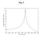
- FIG. 3 shows an example frequency response of a MEMS mirror from a model.
- FIG. 4 shows an exemplary schematic of a general multi-axis controller.
- FIG. 5 shows a prior example which considered combining axis motion in non-linear ways.
- FIGS. 6A and 6B respectively, show position ( 6 A) and velocity ( 6 A) for the axes shown in FIG. 5 .
- FIGS. 7A and 7B respectively, show scan beam acceleration ( 7 A) and Jerk ( 7 B) plots for the axes shown in FIG. 5 .
- FIG. 8 shows an acceleration plot for an exemplary 3-piece cubic spline.
- FIGS. 9A and 9B respectively, show exemplary position ( 9 A) and velocity ( 9 B) for a MEMS-SLID “reverse” or retro-scan move.
- FIGS. 10A and 10B respectively, show exemplary acceleration ( 10 A) and Jerk ( 10 B) curves for the MEMS-SLID “reverse” or retro-scan beam move shown in FIG. 9 .
- the aforementioned Patent Application Ser. No. 61/534,604 disclosed a method for adapting a conventional, general-purpose multi-axis motion controller to produce the desired scan paths.
- the prior disclosed method included control of the nominal beam scan path in the X-Y plane, and control of the parameters of superimposed oscillation properties such as amplitude, frequency, direction, and phase.
- the prior disclosed multi-axis motion controller was designed to produce motion that is smooth not only in value (position) but also in 1 st and higher order rates of change (e.g., velocity, acceleration, and like parameters). This is because the scanning mirror used in certain MEMS-SLID biosensor scanning platforms may have a high tendency to resonate if excited at certain frequencies.
- Discontinuities in motion, and parameters of oscillation are known to produce such frequencies. Discontinuities in rates of change can also produce such frequencies, but the effect lessens with the order in which the discontinuity occurs. Thus, a discontinuity in position has greater impact than in velocity, and a discontinuity in velocity has greater impact than acceleration, and so on.
- FIG. 1 schematically shows a MEMS-SLID reader used to interrogate a LID biosensor, for example, for drug discovery.
- the MEMS-SLID technology used in certain LID readers was disclosed in WO 2011/017147 A1.
- This interrogation method scans an oscillating measurement beam over the biosensors on a plate.
- the use of oscillation is fundamental to reader operation, and is also used to calibrate the system using the methods contained in the aforementioned patent application No. 61/445,266.
- a light source inside a transceiver module produces a small spot of broad spectrum infrared (IR) light on the microplate.
- IR infrared
- a two-dimensional mirror scans the spot over one or more of the sensors on the plate.
- a spectrometer in the transceiver module observes the reflection.
- an objective lens 280 i.e., an f-theta lens
- FIG. 2 shows an exemplary MEMS-SLID scan path used in the disclosed inventive system and method for a sample having six wells.
- the scan path can begin in the center of the plate region (vertex), the move to the starting point of the first scan (“top left”) to sequentially scan the top three wells (circles) having biosensors (squares) and having two rapid motions (or “jumps”) in between adjacent wells.
- the scan path can then change direction (e.g., turns a “corner”) to repeat the process in the reverse X direction before “leading out”.
- the sinusoidal oscillation frequency is constant throughout.
- the baseline (center of oscillatory) motion is shown as a bold line in the center of the oscillation.
- FIG. 3 shows an example frequency response of a MEMS mirror from a model.
- the resonant frequency is 120 Hz and the Q-factor (i.e., response level at resonance) is 100 ⁇ the amplitude of the non-oscillatory response, which is equivalent to +40 dB (power).
- FIG. 4 shows a schematic of a general multi-axis controller, shown here to illustrate a two-axis example.
- An example is shown in the embedded table where an application specifies motion “commands” or moves in polar coordinates (r, ⁇ ) between two consecutive points in time for selected times (t) and observes the motion on a Cartesian (X-Y) gantry.
- FIG. 5 shows an example from the aforementioned Patent Application Ser. No. 61/534,604, which considered combining axis motion in non-linear ways, in particular, to control paths with oscillation in certain LID readers.
- the Texas Instruments TALP1000B MEMS mirror used in certain Corning MEMS-SLID systems has a resonant frequency in the range of 120 Hz and a resonant response over 100 times that of non-oscillatory situation. A typical response for this device is shown in FIG. 5 .
- Many alternative devices that are capable of both tracing non-oscillatory curves with relatively rapid oscillation have low resonant frequencies (Q-points) and high resonant response (Q-factor) compared with “traditional” motion systems, such as industrial automation. Such devices necessarily have an extremely light load compared with the motion force (e.g., from the electromagnets).
- Galvanometers or related devices such as voice-coils are examples.
- FIGS. 6A and 6B respectively, show position ( 6 A) and velocity ( 6 A) for the axes shown in FIG. 5 .
- the move starts at time 0.05 seconds and ends at 0.15 seconds.
- FIGS. 7A and 7B respectively, show scan beam acceleration ( 7 A) and Jerk ( 7 B) plots for the axes shown in FIG. 5 .
- the move starts at time 0.05 seconds and ends at 0.15 seconds.
- a 3-piece cubic form is evident from inspection of the plots.
- FIG. 8 shows an acceleration plot for an exemplary 3-piece cubic spline ( 800 ).
- Jerk is the slope of acceleration, in this instance consisting of three (3) piecewise constants whose time intervals are labeled Cubic 1 ( 810 ), 2 ( 820 ), and 3 ( 830 ).
- FIGS. 9A and 9B respectively, show exemplary position ( 9 A) and velocity ( 9 B) for a MEMS-SLID “reverse” or retro-scan move.
- the start and end positions are the same, in this instance, arbitrarily shown as 0 mm.
- Velocity in the reverse direction retains its magnitude, and the initial and final acceleration are zero.
- the solid line is a 3-piece cubic spline that uses fixed timing apportioning (“Candidate 3F”) and the dotted line is a 2-piece cubic spline using variable time apportioning (“Candidate 2F”).
- FIGS. 10A and 10B respectively, show exemplary acceleration ( 10 A) and Jerk ( 10 B) curves for the MEMS-SLID “reverse” or retro-scan beam move shown in FIG. 9 .
- the solid line is a 3-piece cubic spline using fixed timing apportioning (“Candidate 3F”), and the dotted line is a 2-piece cubic spline using variable time apportioning (“Candidate 2F”). Observe that the 2-piece cubic spline move minimizes absolute jerk magnitude, while the 3-piece cubic spline move has lower internal jerk discontinuity.
- Algorithms for general purpose control are generally known (see for example, Nguyen, et. al., “On Algorithms for Planning S-curve Motion Profiles,” International Journal of Advanced Robotic Systems , Vol. 5, No. 1, 2008, pp. 99-106.), although these algorithms can become complex if velocity and acceleration end points need to be controlled. If so, expensive state-of-the-art controllers may be necessary. Such functions are necessary in certain MEMS-SLID readers, for example, the scanning beam must move in a constant velocity mode to scan across wells, and move rapidly point-to-point between wells while starting and ending with the scan velocity to avoid a sudden jump in speed.
- the system includes a multi-axis motion controller for controlling motion parameters of MEMS mirrors, or like devices.
- the application i.e., master control software
- the motion controller supplies:
- the controller is programmed to calculate a piecewise cubic function, referred to herein as a “plan,” for each axis that meets all the specified conditions.
- This plan can be appended to any current plan, including the case where the current plan is in progress but has not been completed.
- the controller is programmed to evaluate the plan in successive increments of time.
- Axis value e.g., position
- velocity and acceleration are digitally output to post-processing steps such as control loops for position, velocity, or combinations thereof, to control oscillation.
- An example of a unit period function is the sine function.
- any variables x 0 , x 1 , f, and ⁇ may be separate axes under control, specified and computed using the previously mentioned plan.
- (x 0 , y 0 ) is a two-dimensional center of oscillation
- (x 1 , y 1 ) is a vector representing magnitude and direction of oscillation
- f and ⁇ are respectively the frequency and phase of oscillation common to both dimensions.
- This calls for a six-axis motion controller capable of simultaneously evaluating and outputting six plans, which are coordinated with each other because each plan is specified in terms of time, which is common.
- the disclosed system and method are advantaged in several respects including, for example:
- Decreased move time the system and method can perform fast moves between biosensors without causing significant vibration.
- the system and method can reduce vibration, which can improve measurement repeatability or reproducibility.
- the system and method can be readily implemented in new or existing scanning readers.
- the system and method permit a relatively inexpensive motion control processor to be selected because of the realized reduction in memory, and reduction in real-time and non-real time processing.
- the disclosure provides a method for scanning a light beam spot over one or more biosensors supported by a microplate with an optical scanner system having:
- the additional points in time, together with the state of the beam spot at each additional point in time together with the 1 st through the (n ⁇ 1) th order rates of change of the state of the beam spot can be appended to a scan path that is in progress.
- the piecewise polynomial function can be, for example, a cubic spline.
- the piecewise polynomial function can be, for example, of the 3 rd order and has 3-pieces.
- the polynomial function is substantially continuous throughout in axis value and the 1 st through the (n ⁇ 1) th order rates of change.
- the polynomial in between each pair of consecutive points in time can be, for example, calculated using a method that minimizes the maximum discontinuity in the n th order rate of change for a section of the scan path.
- the section of the scan path can include, for example, the entire scan path.
- the defined axes can be combined mathematically to form x and y positions, for example, according to the methods used in aforementioned U.S. Patent Application 61/534,604.
- the elapsed times can be, for example, representative of elapsed time in the real time, the elapsed times can have intervals that are substantially smaller than the smallest interval of the specified selected time series, and the properties can include, for example, at least one of: x position, y position, oscillation amplitude, oscillation direction, oscillation frequency, oscillation phase, and combinations thereof.
- the disclosure provides a system for scanning a light beam spot over one or more biosensors supported by a microplate with an optical scanner system, comprising:
- the elapsed times are representative of elapsed time in real time, the elapsed times have intervals that are substantially smaller than the smallest interval of the series of points in time, and the properties include at least one of: x position, y position, oscillation amplitude, oscillation direction, oscillation frequency, oscillation phase, and combinations thereof.
- the system can further include first and second digital amplifiers operably connected to the controller and respectively configured to convert the x and y locations of the scan path to drive output positions x and y, and to amplify the drive output positions x and y.
- the amplified drive output positions x and y can be, for example, respective x and y currents or voltages.
- the scanning optical system can include, for example, one of a scanning galvanometer, a flexure-based scanning mirror, a micro-electro-mechanical system (MEMs) mirror, an oscillating plane mirror, a rotating multifaceted mirror, and a piezo-electric-driven mirror.
- a scanning galvanometer a flexure-based scanning mirror
- MEMs micro-electro-mechanical system
- oscillating plane mirror a rotating multifaceted mirror
- a piezo-electric-driven mirror for example, one of a scanning galvanometer, a flexure-based scanning mirror, a micro-electro-mechanical system (MEMs) mirror, an oscillating plane mirror, a rotating multifaceted mirror, and a piezo-electric-driven mirror.
- MEMs micro-electro-mechanical system
- system can further include, for example, a system controller operably connected to the motion controller and configured to input the series of points in time, and at each point in time the value of each scan path property and the 1 st through the (n ⁇ 1) th order rate of change of each of the properties to the multi-axis controller.
- a system controller operably connected to the motion controller and configured to input the series of points in time, and at each point in time the value of each scan path property and the 1 st through the (n ⁇ 1) th order rate of change of each of the properties to the multi-axis controller.
- FIG. 4 illustrates the operation of a simple, two-axis motion controller.
- an external software application (“application”) controls axes in two-dimensional polar coordinates to a machine tool on a Cartesian gantry.
- the axes are magnitude r and angle ⁇ .
- the application supplies:
- a specific example of a specification used to generate a motion plate (“plan”) can be:
- the motion controller calculates a plan for each axis.
- the plans are functions of time for both r and ⁇ , and that meet the specifications supplied by the application.
- each plan can be the aforementioned cubic spline.
- a “move” as used herein refers to the segment of a motion plan between two consecutive points in time specified by the application.
- the moves that may be desired for certain MEMS-SLID readers are exemplified in FIG. 2 . All instances can have a zero starting and zero ending acceleration except for blended moves.
- the term “move” here also covers situations such as changing oscillation amplitude, phase, or frequency. There is no mathematical difference between a move in position and oscillation amplitude. The differentiation is only a linguistic attribute and convenience.
- the term “move” also includes changes of value, rate of change of value (velocity), and 2 nd order rate of change of value (acceleration).
- a move includes the segments of the motion plan for all the axes. Therefore, a move may be between points in X-Y space, and may include changes in oscillation amplitude, direction, frequency, and phase.
- “Scanning” a beam across a biosensor is move that may call for a difference in non-oscillatory position, constant velocity, and no changes in other parameters. As the scan may be angled slightly to match biosensor orientation, this can involve a change in both X and Y.
- “Skipping” a beam between wells is a move that may call for a difference in position, the same start velocity and end velocity, and having rapid acceleration in between. For scanning, this can involve X and Y.
- Reversing direction is a move that may need a change in direction, in velocity, and can have the same non-oscillatory start and end point. In the example of FIG. 2 , reversing is shown in the X direction after the end of the first row scan of biosensors and the start of the second row scan of biosensors.
- Point-to-point moves require a change in position, where the start and end velocity are zero.
- reversing is shown in the Y direction after the end of the first row scan of biosensors and the start of the second row scan of biosensors.
- changes in oscillation amplitude also fall into this category.
- a point-to-point move is a special instance of a “skip”, where the start and the end velocities are zero.
- “Ramps” are moves at the start and again at end of the scan, where the position changes and the velocity changes, such as either from zero to the scan speed, or from the scan speed back to zero. In MEMS-SLID readers, this can occur in the X and Y direction at the start and at the end of a scan. Note that the oscillation amplitude change can occur simultaneously and is categorized as a point-to-point move.
- Blend When any move is aborted prior to completion, a blended move may be appended from the current position to the start of the next move. This might happen, for example, during a search where a feature has been found. Typically neither the initial and final position nor the initial and final velocity is equal. In addition, the initial acceleration is typically non-zero. The final acceleration is specified by the next move in the plan (as above) and typically will be zero.
- Blended moves are not necessary to implement MEMS-SLID readers, but can be desirable in other systems. Blended moves are the only moves in MEMS-SLID with non-zero initial acceleration. All moves in the disclosed MEMS-SLID system have zero final acceleration.
- a main task of the motion controller of the disclosure is to determine a value, such as by calculation, and if called for a 1 st and a 2 nd order rate of change, at a sequence of successive times defined by a controller update rate.
- This collection or sequence of points forms the “motion path”.
- the time interval between these calculated points can typically be many orders of magnitude less than that of the specific application.
- an update of each axis can be, for example, at up to 50 kHz.
- the MEMS-SLID application software specifies conditions at, at for example, up to 200 time points (199 moves) over 120 seconds, with intervals between time points varying, for example, from 0.01 to 5 seconds, from 0.02 to 4 seconds, from 0.03 to 3 seconds, from 0.04 to 2 seconds, including intermediate values and ranges.
- the microprocessor selected for the design one of the highest end processors in its class but still inexpensive at $17, has only 512 Kbytes of memory
- An overarching strategy of the disclosure is to specify the scan beam motion path as a table of functions for each axis.
- a cubic spline type function can be selected. This function is a piecewise cubic having up to three pieces per axis for each move. The total memory required is 48 bytes per axis per move (4 coefficients, 32-bits each, 3 pieces), or 56 kbytes, for the 6-axes, 200 application-specified point path mentioned in the example above.
- a cubic spline was selected because it can be made to meet all the necessary conditions while maintaining continuity in position, velocity, and acceleration.
- Cubic forms are a common form in industrial controllers because it is known that the 3 rd order derivative is related to machine tool wear and hence needs to be controlled. That justification is irrelevant in the present disclosure's applications. However, modeling and experimentation both showed that small discontinuities in the 3 rd order derivative had an acceptably small impact.
- FIG. 4 shows a schematic of the custom control system including a multi-axis controller embodying the disclosed method.
- the control system can include, for example:
- control system and method can perform one or more of the following functions or operations:
- the strategy used in the disclosure is to calculate the section of the scan path for a single-axis move between two application specified time points in isolation. Continuity of the overall path in position, and in the 1 st and 2 nd order rates of change is guaranteed because the end time of one move is the start of time of the next move; every move then shares data with both the previous and next move.
- the application coordinates an arrangement of axes, if required, by specifying start and end points for the axes at the same time.
- each move (and therefore the overall path) is a piecewise n th -order polynomial function that is globally continuous in up to the (n ⁇ 1) th order rate of change (mathematically, the entire path is n ⁇ 1 times continuously differentiable).
- a piecewise function with these properties is known in mathematics as a “spline”.
- the application requires continuity in the n th order rate of change, the application specifies the start and end axis rates of change up to the n th order, and an (n+1) th order spline is called for.
- This disclosure primarily describes the cubic spline (i.e., 3 rd order) because a cubic is the lowest order polynomial capable of describing continuous acceleration (the 2 nd order rate of change above).
- Relative time is defined to be zero at the start of any piece. Relative time is easily related to time as specified by the application, because the length of time for which each cubic piece is valid is included as part of the spline definition.
- Each move can be constructed as a cubic spline with one to three pieces (within the overall cubic spline). The pieces are easy to identify in acceleration and jerk plots.
- FIG. 8 shows an example of acceleration for a 3-piece spline.
- Equation 1.1 An example formulation for the n th cubic piece in a spline is provided in Equation 1.1, where the variable s is used for value or position.
- the 1 st to 3 rd order derivatives (of time), referred to respectively as velocity v, acceleration a, and jerk J are shown for convenience:
- Equation 1.1 The cubic form for Equation 1.1 is arbitrary, and as mentioned previously this method may be extended to higher orders.
- the 3 rd order time derivative is referred to herein as “jerk”.
- the (kinematic) equation of motion was selected so that the coefficients s0, v0, a0, and Jn have the standard physical meanings of position, velocity, acceleration, and jerk respectively.
- Constants before coefficients e.g., the 1 ⁇ 6 before Jn ⁇ t 3
- n The “n” following quantities s, v, a, J, and T denote the n th cubic piece for that move. Subsequently, this “n” is often written as an explicit number.
- the postscript “n” is used only for understanding and readability, and is omitted in cases where the quantity in question is not generally compared between different cubic pieces. For example, s 0 in Eq. 1.1 is technically s 0 n because s 0 is different for each cubic piece.
- Jn The “0” subscript is omitted from the jerk coefficient (Jn) because Jn is the constant value of jerk for all time in the range T to Tn, so Jn is more than just an initial condition.
- Jn the “n” following Jn is included because this quantity is often compared between cubic pieces.
- the completion time T1 is the application specified move time T. Only J1 is free for meeting the three remaining (end) conditions s F , v F , and a F and a general solution is not possible. There are degenerate conditions for which a solution is possible.
- Two exemplary methods (among others) are provided that can be used to construct closed form solutions to the problem of specifying a spline for moves.
- the two methods presented both assume the number of cubic pieces N is determined.
- a first method applies when the validity times Tn for the polynomial pieces are not pre-determined.
- Step 1 The application specified initial conditions (e.g., s I , v I , a I ) automatically set all the coefficients except the highest order coefficient (e.g., s 0 , v 0 , a 0 ) for the first polynomial (e.g., cubic) as mentioned previously.
- the highest order coefficient (J1 for a cubic) and T1 are to be determined.
- Step 2 Use continuity between the last determined polynomial piece and the next piece in position and each rate of change to find the next set of coefficients (s 0 , v 0 , a 0 ) (for a cubic) in terms of the specified variables s I , v I , a I and previous to-be-determined variables Tn and (for a cubic) Jn. Repeat this step for each piece in succession.
- the result of the first method are three simultaneous equations expressed in terms of the application defined initial and final axis values and rates of change (e.g., s I , v I , a I , s F , v F , a F ), the move time T, the free higher-order coefficients (the Jn for cubic pieces), and the variables Tn for all but the last piece.
- T ⁇ ⁇ 1 ⁇ ⁇ ⁇ v + 3 ⁇ ⁇ ⁇ ⁇ v 2 ⁇ ⁇ ⁇ ⁇ v ⁇ T - 3 ⁇ ⁇ ⁇ ⁇ s ⁇ ⁇ ⁇ v
- a two piece cubic can however represent a reverse in direction, and in that case is in a sense an optimal cubic form for minimizing jerk.
- T1 (from above) is given below with J1 and J2.
- This solution has optimal continuity in that it minimizes worst case discontinuity with the moves on either side.
- the only discontinuity in the cubic spline formulation of the disclosure is in jerk. Jerk is constant for every piece, but discontinuous at piece boundaries. In this particular instance, jerk for the two pieces is symmetrical about zero having equal magnitude, and opposite signs. This minimizes the absolute magnitude of jerk, which in turn minimizes the worst-case discontinuity at the boundaries with unknown up and down stream moves.
- n-equations e.g., Eq. 3
- n highest order coefficients e.g., n highest order coefficients
- n ⁇ 1 times e.g., n ⁇ 1 times
- J1, J2, J3, T1, and T2 n-equations
- worst-case discontinuity in the highest order coefficient in the cubic case, jerk
- T ⁇ ⁇ 1 T 4
- T ⁇ ⁇ 2 T 2
- T ⁇ ⁇ 3 T 4
- ramps While ramps are not numerous, they are required. It is also desirable to cover blended moves for further applications.
- the application requires a “fall back” solutions that, while not guaranteed to be optimal in minimizing jerk, produces continuous value (position), velocity, and acceleration, and definitely works. It is also desirable that these moves cover the example of non-zero initial acceleration to cover blended moves.
- Step 1 The application specified variables s I , v I , a I automatically set s 0 , v 0 , a 0 for the first cubic.
- the term J1 remains a variable.
- Step 2 Use continuity between the one cubic piece and next cubic piece to find the next s 0 , v 0 , a 0 in terms of the specified variables s I , v I , a I and the to-be-determined variables T and Jn. Repeat this step for each piece in succession.
- An example, for the second cubic is given by:
- one sensible choice of time allocation is to use the values from the previous three piece cubic example that worked for “skip” and “point-to-point” moves.
- move is actually a skip or point-to-point move
- the general solution will be the same as the already formulated skip move This means the previous skip solution need not be included in the final algorithm.
- time allotments were T/4, T/2, and T/4, respectively, so q1, q2, and q3 are respectively, 4, 2, and 4 in the formulation. This move will be most optimal when it represents the example under which the times allotment was calculated (i.e., skips or point-to-point).
- this method applies to any fixed allotments of time found by solving Eq. 3 for any consideration of conditions, e.g., different ways of assigning jerk, or initial and final application conditions other than those considered here.
- FIGS. 9A and 9B show exemplary position ( 9 A) and velocity ( 9 B) for a MEMS-SLID “reverse” or retro-scan move and plots of a reverse move.
- the two- and three-piece variable time methods both give the same solution.
- the three-piece version is degenerate.
- the three-piece fixed time method gives a different solution.
- the three-piece method has lower internal jerk.
- This two-piece move has the lower absolute jerk which minimized jerk discontinuity at the start and down for arbitrary (i.e., unknown) upstream and down stream moves.
- the up and down stream “reverse” moves always scan across wells, where velocity is constant and jerk is zero.
- the three-piece method has the lowest jerk worst case discontinuity in the system (the largest is in the middle of the two-piece move). The discontinuity at the start of the scan (where it affects the process most) is lowest for the two-piece move. It is not apparent, which is the best choice.
- the following procedure calculates a cubic spline between two application supplied points, where the time difference plus the initial and final position, the initial and final velocity, and the initial and final acceleration are given as: T, s I , s F , v I , v F , a I , and a F .
- candidates for all moves in an application specified path can be calculated a priori then select the set of candidates that minimize worst case discontinuity in jerk by examining the values of Jn for each potential cubic piece in the overall spline. If using a higher order polynomial, minimize discontinuity at piece boundaries in the highest order polynomial coefficient. Otherwise, find the maximum magnitude jerk for each candidate, and select candidates to minimize that quantity.
Landscapes
- Physics & Mathematics (AREA)
- General Physics & Mathematics (AREA)
- Optics & Photonics (AREA)
- Spectroscopy & Molecular Physics (AREA)
- Health & Medical Sciences (AREA)
- Life Sciences & Earth Sciences (AREA)
- Chemical & Material Sciences (AREA)
- Analytical Chemistry (AREA)
- Biochemistry (AREA)
- General Health & Medical Sciences (AREA)
- Immunology (AREA)
- Pathology (AREA)
- Apparatus Associated With Microorganisms And Enzymes (AREA)
Abstract
-
- defining a scan path for an optical scanner including selecting axes representing properties of the scan path and selecting a time series, calculating a piecewise polynomial function of time between each point in the time series; and
- scanning the light beam spot over one or more biosensors according to the defined scan path, as described herein.
Description
-
- a series of points in time;
- a specified value of that axis at each point in time (e.g., position, oscillation amplitude);
- a 1st order rate of change of the value at each point in time (e.g., velocity, rate of change of amplitude); and
- a 2nd order rate of change of the value at each point in time (e.g., acceleration).
Multiple axes are coordinated and use time as a common variable. In embodiments, the series of points in time may be the same for all axes under consideration.
-
- a smoothness order n;
- a set of properties that describe the x and y position of the beam spot at any time;
- a series of points in time and at each point in time a value for each of the properties and the 1st through the (n−1)th order rates of change of each of the properties;
- the method comprising:
- defining an axis for each property used to describe the state of the beam spot;
- calculating for each axis an nth order piecewise polynomial function of time between each point in the series of points in time that equals the specified axis value and the 1st through the (n−1)th order rates of change;
- producing a series of elapsed times between each point in the series of points in time;
- calculating each axis value from the polynomial function at each point in the series of elapsed times;
- calculating the x and y locations of the scan path from the axis values at each point in time; and
- sending the calculated x and y locations to the scanning optical system when each point in elapsed time series occurs to cause the scanning optical system to deflect the light beam and scan the beam spot over the defined scan path.
-
- there are n polynomial pieces, and the duration of each of the polynomial pieces are fixed ratios of the total duration between the points in time;
- there are n polynomial pieces, where the highest order coefficient of the n polynomial pieces have substantially the same absolute value, and the duration of each polynomial piece is a calculated parameter; or
- the polynomial is of the 3rd order, there are two polynomial pieces, and the 3rd order coefficient and duration of each piece are calculated parameters.
-
- a motion controller configured to:
- receive a series of points in time, and at each point in time the value of each scan path property and the 1st through the (n−1)th order rate of change of each of the properties;
- calculate a series of elapsed points in time between each received point in time; and
- calculate the x and y locations of the scan path at each point of elapsed points in time as defined for the above described method; and
- an optical scanner system configured to receive the x and y locations of the scan path at each elapsed point in time, and thereafter deflect the light beam to scan the beam spot over the scan path.
- a motion controller configured to:
-
- a series of points in time;
- the desired value of r and θ at each point in time;
- a 1st order rate of change of r and θ at each point in time; and
- a 2nd order rate of change of r and θ at each point in time.
-
- (r,θ)=(0 mm, 0°) to (20 mm, 0°) in 0.1 seconds,
- then to (10 mm, 90°) in 0.3 seconds,
- then to (0 mm, 90°) in 0.1 seconds,
- then stop.
Specification of rates of change as mentioned previously have been omitted from the example for clarity, and can be assumed to be zero in the example.
| TABLE 1 |
| Standard measurement cycle listing. |
| X Center | Y Center | X & Y Oscillation | |
| Type | Position | Position | Amplitude |
| Scans | n | n | — |
| Skips | r (c − 1) | r (c − 1) | — |
| Reverses | r − 1 | — | — |
| Point-to-Point | — | r + 1 | 2 |
| | 2 | — | — |
| Null | — | — | 2 n − 1 |
| Total | 2 n + 1 | 2 n + 1 | 2 n + 1 |
Overview of the Method
-
- a microprocessor
- a memory for data;
- an application program;
- two digital-to-analog converters for output of the current position to two current drivers that drive the MEMS mirror; and
- four analog-to-digital converters for capturing position of the MEMS mirror.
-
- contain the application software that generates and continually adds to the move sequence for each application axis;
- continually generates and appends function pieces describing motion to the path;
- continually generates a sequence of times representative of actual elapsed time;
- continually calculates the current value for each application axis;
- indexes through the functions the pieces in sequence as each expires;
- digitally filters the applications axis values;
- combines the application's axis values (e.g., x0, x1, y0, y1, f and θ) to generate physical axis set points (i.e., x and y), for example, using the method disclosed in aforementioned Patent Application Ser. No. 61/534,604;
- converts the physical axis set points into two currents that drive the MEMS mirror; and
- optionally closes a position loop by comparing the physical axis set points with mirror feedback.
Move Definition and Formulation
-
- the start and end times, represented by the relative time difference T (see below);
- the start and end axis value, referred to as “position”, sI and sF; the start and end axis rate of change, referred to as “velocity”, vI and vF; and the start and end
axis 2nd order rate of change, referred to as “acceleration”, aI and aF.
Example having One-Piece Scan Moves
into Eqs. 1.1 to 1.3 and set these equal to the application specified final conditions. That is:
sN(TN)=s F
vN(TN)=v F
aN(TN)=a F (Eqs. 3)
Δs≡s F −s I Σs≡s I +s F Δv≡v F −v I Σv≡v I +v F Δa≡a F −a I Σa≡a I +a F
Example with Two Pieces—Reverse Moves
and so on for velocity and acceleration.
sN(T/qN)=s F
vN(T/qN)=v F
aN(T/qN)=a F (Eqs. 6)
| TABLE 2 | |||||
| Method | “1” | “2T” | “3T” | “3F” | |
| |
1 |
2 |
3 |
3 Piece | |
| Time | — | Variable | Variable | Fixed | |
| Apportioning | |||||
| Jerk | — | Variable | Fixed | Variable | |
| Magnitude | |||||
| Guaranteed | No | No | Yes | Best Method | |
| Solution | |||||
| Scans | Yes | Yes | Yes | Yes | All |
| equivalent | |||||
| Skips | — | — | Yes | Yes | 3T = 3F |
| Reverses | — | Yes | Yes | Yes | 2T = 3T or |
| 3F | |||||
| Point- | — | — | Yes | Yes | 3T = 3F |
| to-Point | |||||
| Ramps | — | — | — | Yes | 3F |
Δs≡s F −s I Σs≡s I s F Δv≡v F −v I Σv≡v I +v F Δa≡a F −a I Σa≡a I +a F
Candidate 3T: Three Piece Variable Time Allotment
Candidate 3X: Three Piece Other
Claims (15)
Priority Applications (1)
| Application Number | Priority Date | Filing Date | Title |
|---|---|---|---|
| US13/753,879 US8922858B2 (en) | 2012-01-31 | 2013-01-30 | Motion axis control and method for biosensor scanning |
Applications Claiming Priority (2)
| Application Number | Priority Date | Filing Date | Title |
|---|---|---|---|
| US201261592901P | 2012-01-31 | 2012-01-31 | |
| US13/753,879 US8922858B2 (en) | 2012-01-31 | 2013-01-30 | Motion axis control and method for biosensor scanning |
Publications (2)
| Publication Number | Publication Date |
|---|---|
| US20130194647A1 US20130194647A1 (en) | 2013-08-01 |
| US8922858B2 true US8922858B2 (en) | 2014-12-30 |
Family
ID=48869979
Family Applications (1)
| Application Number | Title | Priority Date | Filing Date |
|---|---|---|---|
| US13/753,879 Expired - Fee Related US8922858B2 (en) | 2012-01-31 | 2013-01-30 | Motion axis control and method for biosensor scanning |
Country Status (1)
| Country | Link |
|---|---|
| US (1) | US8922858B2 (en) |
Families Citing this family (2)
| Publication number | Priority date | Publication date | Assignee | Title |
|---|---|---|---|---|
| US8922860B2 (en) * | 2011-02-22 | 2014-12-30 | Corning Incorporated | Motion control systems and methods for biosensor scanning |
| JP6134348B2 (en) * | 2015-03-31 | 2017-05-24 | シスメックス株式会社 | Cell imaging device and cell imaging method |
Citations (3)
| Publication number | Priority date | Publication date | Assignee | Title |
|---|---|---|---|---|
| US20030092075A1 (en) * | 2000-10-30 | 2003-05-15 | Sru Biosystems, Llc | Aldehyde chemical surface activation processes and test methods for colorimetric resonant sensors |
| US6586257B1 (en) * | 1999-10-12 | 2003-07-01 | Vertex Pharmaceuticals Incorporated | Multiwell scanner and scanning method |
| US20100231907A1 (en) * | 2000-10-30 | 2010-09-16 | Sru Biosystems, Llc | Method and Apparatus for Biosensor Spectral Shift Detection |
-
2013
- 2013-01-30 US US13/753,879 patent/US8922858B2/en not_active Expired - Fee Related
Patent Citations (3)
| Publication number | Priority date | Publication date | Assignee | Title |
|---|---|---|---|---|
| US6586257B1 (en) * | 1999-10-12 | 2003-07-01 | Vertex Pharmaceuticals Incorporated | Multiwell scanner and scanning method |
| US20030092075A1 (en) * | 2000-10-30 | 2003-05-15 | Sru Biosystems, Llc | Aldehyde chemical surface activation processes and test methods for colorimetric resonant sensors |
| US20100231907A1 (en) * | 2000-10-30 | 2010-09-16 | Sru Biosystems, Llc | Method and Apparatus for Biosensor Spectral Shift Detection |
Also Published As
| Publication number | Publication date |
|---|---|
| US20130194647A1 (en) | 2013-08-01 |
Similar Documents
| Publication | Publication Date | Title |
|---|---|---|
| Leusin et al. | Solving the job-shop scheduling problem in the industry 4.0 era | |
| McConachie et al. | Manipulating deformable objects by interleaving prediction, planning, and control | |
| Lindström et al. | An initial model for zero defect manufacturing | |
| Gia Luan et al. | Real-time hybrid navigation system-based path planning and obstacle avoidance for mobile robots | |
| Yu et al. | Positioning, navigation, and book accessing/returning in an autonomous library robot using integrated binocular vision and QR code identification systems | |
| Farias et al. | A neural network approach for building an obstacle detection model by fusion of proximity sensors data | |
| Hercik et al. | Implementation of autonomous mobile robot in smartfactory | |
| Li et al. | Welding seam trajectory recognition for automated skip welding guidance of a spatially intermittent welding seam based on laser vision sensor | |
| US8922858B2 (en) | Motion axis control and method for biosensor scanning | |
| Minnetti et al. | A smartphone integrated hand-held gap and flush measurement system for in line quality control of car body assembly | |
| Schmitz et al. | A robot-centered path-planning algorithm for multidirectional additive manufacturing for WAAM processes and pure object manipulation | |
| Gogolák et al. | Wireless sensor network aided assembly line monitoring according to expectations of industry 4.0 | |
| Chen et al. | H∞ robust control of a large-piston MEMS micromirror for compact fourier transform spectrometer systems | |
| Bucinskas et al. | Improving industrial robot positioning accuracy to the microscale using machine learning method | |
| Pérez-Ubeda et al. | Force control improvement in collaborative robots through theory analysis and experimental endorsement | |
| Heydarzadeh et al. | Experimental kinematic identification and position control of a 3-DOF decoupled parallel robot | |
| Fang et al. | A vision-based robotic laser welding system for insulated mugs with fuzzy seam tracking control | |
| Cibicik et al. | Laser scanning and parametrization of weld grooves with reflective surfaces | |
| Gyenes et al. | Can genetic algorithms be used for real-time obstacle avoidance for lidar-equipped mobile robots? | |
| Zhu et al. | A novel fractional order model for the dynamic hysteresis of piezoelectrically actuated fast tool servo | |
| Zhang et al. | A GAN-BPNN-based surface roughness measurement method for robotic grinding | |
| Van Pham et al. | Hybrid spiral STC-hedge algebras model in knowledge reasonings for robot coverage path planning and its applications | |
| IL294522A (en) | System and method for controlling automatic inspection of articles | |
| Magalhaes et al. | Inspection application in an industrial environment with collaborative robots | |
| Cao et al. | Online optimization method for nonlinear model-predictive control in angular tracking for MEMS micromirror |
Legal Events
| Date | Code | Title | Description |
|---|---|---|---|
| AS | Assignment |
Owner name: CORNING INCORPORATED, NEW YORK Free format text: ASSIGNMENT OF ASSIGNORS INTEREST;ASSIGNOR:TOVEY, CAMERON JOHN;REEL/FRAME:029721/0406 Effective date: 20130130 |
|
| FEPP | Fee payment procedure |
Free format text: MAINTENANCE FEE REMINDER MAILED (ORIGINAL EVENT CODE: REM.); ENTITY STATUS OF PATENT OWNER: LARGE ENTITY |
|
| LAPS | Lapse for failure to pay maintenance fees |
Free format text: PATENT EXPIRED FOR FAILURE TO PAY MAINTENANCE FEES (ORIGINAL EVENT CODE: EXP.); ENTITY STATUS OF PATENT OWNER: LARGE ENTITY |
|
| STCH | Information on status: patent discontinuation |
Free format text: PATENT EXPIRED DUE TO NONPAYMENT OF MAINTENANCE FEES UNDER 37 CFR 1.362 |
|
| FP | Expired due to failure to pay maintenance fee |
Effective date: 20181230 |