US8060338B2 - Estimation of global position of a sensor node - Google Patents
Estimation of global position of a sensor node Download PDFInfo
- Publication number
- US8060338B2 US8060338B2 US12/025,160 US2516008A US8060338B2 US 8060338 B2 US8060338 B2 US 8060338B2 US 2516008 A US2516008 A US 2516008A US 8060338 B2 US8060338 B2 US 8060338B2
- Authority
- US
- United States
- Prior art keywords
- sensor node
- data
- trajectory information
- coordinates
- information data
- Prior art date
- Legal status (The legal status is an assumption and is not a legal conclusion. Google has not performed a legal analysis and makes no representation as to the accuracy of the status listed.)
- Expired - Fee Related, expires
Links
Images


Classifications
-
- G—PHYSICS
- G01—MEASURING; TESTING
- G01S—RADIO DIRECTION-FINDING; RADIO NAVIGATION; DETERMINING DISTANCE OR VELOCITY BY USE OF RADIO WAVES; LOCATING OR PRESENCE-DETECTING BY USE OF THE REFLECTION OR RERADIATION OF RADIO WAVES; ANALOGOUS ARRANGEMENTS USING OTHER WAVES
- G01S5/00—Position-fixing by co-ordinating two or more direction or position line determinations; Position-fixing by co-ordinating two or more distance determinations
- G01S5/02—Position-fixing by co-ordinating two or more direction or position line determinations; Position-fixing by co-ordinating two or more distance determinations using radio waves
- G01S5/0284—Relative positioning
- G01S5/0289—Relative positioning of multiple transceivers, e.g. in ad hoc networks
-
- G—PHYSICS
- G01—MEASURING; TESTING
- G01S—RADIO DIRECTION-FINDING; RADIO NAVIGATION; DETERMINING DISTANCE OR VELOCITY BY USE OF RADIO WAVES; LOCATING OR PRESENCE-DETECTING BY USE OF THE REFLECTION OR RERADIATION OF RADIO WAVES; ANALOGOUS ARRANGEMENTS USING OTHER WAVES
- G01S5/00—Position-fixing by co-ordinating two or more direction or position line determinations; Position-fixing by co-ordinating two or more distance determinations
- G01S5/02—Position-fixing by co-ordinating two or more direction or position line determinations; Position-fixing by co-ordinating two or more distance determinations using radio waves
- G01S5/0205—Details
- G01S5/0221—Receivers
- G01S5/02213—Receivers arranged in a network for determining the position of a transmitter
-
- G—PHYSICS
- G01—MEASURING; TESTING
- G01S—RADIO DIRECTION-FINDING; RADIO NAVIGATION; DETERMINING DISTANCE OR VELOCITY BY USE OF RADIO WAVES; LOCATING OR PRESENCE-DETECTING BY USE OF THE REFLECTION OR RERADIATION OF RADIO WAVES; ANALOGOUS ARRANGEMENTS USING OTHER WAVES
- G01S5/00—Position-fixing by co-ordinating two or more direction or position line determinations; Position-fixing by co-ordinating two or more distance determinations
- G01S5/18—Position-fixing by co-ordinating two or more direction or position line determinations; Position-fixing by co-ordinating two or more distance determinations using ultrasonic, sonic, or infrasonic waves
Definitions
- the present disclosure is generally related to determining the absolute position of a sensor node, and more specifically to determining the absolute position of a sensor node that has been disposed in a haphazard manner.
- the present disclosure pertains to the field of localization of sensors.
- Sensors are usually deployed in a region to observe the activity in an area of interest. Different sensors are deployed to observe different activity.
- Acoustic sensors are deployed in a battlefield or in an urban area to monitor acoustic activity, for example, the presence of tanks in the field, to track vehicles, and identify the type of vehicles, etc.
- acoustic sensors can be deployed to detect congregation of people and the general nature of such a congregation, that is, whether the crowd is hostile or peaceful.
- the deployed acoustic sensors record the sound waves emanated in the vicinity and transmit to a remote hub or a central observation center where the data (sound waves) is analyzed.
- the type of analysis employed depends on the type of activity for which one is looking.
- Tracking vehicles in a field may comprise use of a tracking algorithm, while detecting people in the field may require an entirely different algorithm.
- the data analyzed has to be referenced to the location of the sensor. Without the knowledge of the sensor location, the data has no relevance.
- the sensors may be deployed using an airborne vehicle such as a helicopter or airplane, or the sensors can be deployed by rockets. Whatever mechanism is used for deploying the sensors, the location of the deployed sensors may not be available. It is possible to guess at the general vicinity where the sensors land based on the location of the deploying vehicle, the speed at which the vehicle was flying, the angle at which the sensors were hurled, general wind speeds in the vicinity, the direction in which the vehicle was traveling, etc.
- the present disclosure presents a robust and elegant means in determining the location of the sensors.
- localization methods e.g., R. L. Moses, R. M. Patterson, and W. Garber, Self localization of Acoustic sensor networks”, in Proc. of MSS meeting of the specialty group on Battlefield acoustic and seismic sensing, September 2002 include use of beacons to estimate the time of arrival (TOA) between two sensor nodes, which translates into range after multiplying the TOA with the propagation velocity of the signal in the medium.
- TOA time of arrival
- an apparatus and method for locating a sensor node are provided.
- a processing unit that receives sensor node data and object trajectory information data for an object.
- the sensor node data is related to the object from which the bearings of the object can be estimated which in turn are related to the trajectory of the object, and a data point in the object trajectory information data comprises a time stamp and the coordinates of a position.
- the position corresponds to the location of the object at the given time.
- the processing unit is adapted to use several bearing estimates from the sensor node data and the corresponding position information of the object to determine an absolute position of the sensor node.
- An embodiment of a method can be broadly summarized by the following: collecting object trajectory information data for an object, wherein the object trajectory information data is collected over a time span; acquiring sensor node data at the sensor node, wherein the sensor node data is acquired over the same time span and is related to the object trajectory information data; determining several direction indicators, each direction indicator providing an approximate bearing from the sensor node to the object at a given instant of time during the time span the data is collected; and determining coordinates of the sensor node using a portion of the collected trajectory information data and the corresponding direction indicators (bearings) determined by the sensor node data.
- FIG. 1 is a block diagram of a detection system including an array of sensor nodes and a central observation center.
- FIGS. 2A-2C are block diagrams of embodiments of sensor nodes of FIG. 1 .
- FIG. 3 is a block diagram of the sensor node of FIG. 2A .
- FIG. 4 is an exemplary flow chart of a method for locating a sensor node.
- FIG. 5 is diagram of trajectory path over the array of sensor nodes of FIG. 1 .
- FIG. 6A is a diagram of sensor node data.
- FIG. 6B is a diagram of the frequency spectrum of the sensor node data of FIG. 6A .
- FIG. 7 is an exemplary flow chart of a method for determining sensor node bearing angles.
- FIG. 8 is an exemplary flow chart of a method for locating a sensor node.
- FIG. 9 is a diagram of triangulating on the location of a sensor node.
- FIGS. 10A and 10B illustrate a process for locating a sensor node using geometric and trigonometric relationships.
- FIGS. 11A and 11B illustrate the grid structure used to refine the sensor location from an initial estimate of the sensor location.
- a detection system 10 includes a central observation center (COC) 12 and a sensor array 14 , which is disposed over a region 16 .
- the sensor array 14 includes a plurality of sensor nodes 18 , which are adapted to detect objects 20 including natural objects and man-made objects.
- the sensor nodes 18 communicate data 22 regarding detected objects 20 to the COC 12 via a wireless communication link 24 .
- the data 22 typically includes a sensor node identifier and a direction indicator, i.e., the angular direction of the detected object from the sensor node 18 .
- data 22 includes raw data or partially-processed data, and generally includes the sensor node identifier.
- the COC 12 includes a processing unit 26 that processes the data 22 to determine, among other things, the absolute or global coordinates of the sensor node 18 , and/or to identify the detected object 20 .
- the sensor nodes 18 passively detect energy 27 that is emitted from the object 20 .
- energy 27 that is emitted from the object 20 .
- Non-limiting examples of the types of energy 27 that the sensor nodes 18 are adapted to detect include electromagnetic energy and acoustic energy.
- the spectrum of electromagnetic energy includes both visible light and non-visible light, such as infrared, and that acoustic energy is not limited to sounds carried by a gaseous medium, such as the Earth's atmosphere, and is medium independent. In other words, acoustic energy can be carried by a gas, solid, or a liquid medium.
- the sensor nodes 18 are disposed over the region 16 in a haphazard or essentially random, unpredictable manner.
- the sensor nodes 18 can be delivered, among other methods of deployment, to the region 16 by an artillery shell and/or mortar shell, by dropping from one or more aerial vehicles, by dropping from ships and/or submarines, by dropping from a ground vehicle, and/or by dropping by personnel.
- FIGS. 2A-2C illustrate different, non-limiting embodiments of a sensor node 18 ( a ), 18 ( b ), and 18 ( c ), respectively.
- Each of the sensor nodes 18 ( a ) through 18 ( c ) include a plurality of sensors 28 and a central unit 30 .
- Sensor node 18 ( a ) includes three sensors 28 , which are disposed on the ground 31 in an approximate equiangular distribution about the central unit 30 .
- sensors 28 are microphones.
- Sensor node 18 ( b ) includes four sensors 28 disposed on the ground 31 in an approximate equiangular distribution about the central unit 30 , and one sensor 28 ( d ), which is elevated off of the ground 31 by a support member 32 .
- the support member 32 extends generally upward from the central unit 30 .
- Sensor node 18 ( c ) includes a plurality of sensors 28 that are approximately linearly aligned. It should be remembered that sensor nodes 18 ( a ) through 18 ( c ) are non-limiting examples and that, in other embodiments, greater or fewer sensors can be employed and/or the sensors can be deployed about the central unit in other configurations such as essentially random, non-equiangular, etc.
- FIG. 3 illustrates selected components of the sensor node 18 ( a ).
- the central unit 30 includes a preamplifier 34 , a filter 36 , an analog/digital converter (A/D) 38 , a direction estimator 40 , and a transmitter 42 .
- Sensors 28 ( a )- 28 ( c ) receive energy 27 (for example, helicopter sound in the case of acoustic sensors) and convert the energy into electrical signals, which are then provided to the preamplifier 34 via electrical connectors 44 (A)- 44 (C). Electrical signals from the sensors 28 ( a )- 28 ( c ) are processed by the preamplifier 34 , filter 36 , and A/D converter 38 independently.
- the preamplifier 34 amplifies the electrical signals and provides them to the filter 36 .
- the filter 36 is an anti-aliasing filter (low-pass filter at half the sampling frequency) that filters unwanted noise from the electrical signals and provides the electrical signals to the A/D converter 38 , which digitizes the electrical signals.
- an anti-aliasing filter low-pass filter at half the sampling frequency
- the direction estimator 40 receives and processes the digitized electrical signals.
- the direction estimator 40 includes a high-resolution direction of arrival angle estimator, namely, a minimum variance distortionless response (MVDR) (Van Veen, B. D., and K. M. Buckley, “Beamforming: a versatile approach to spatial filtering,” IEEE ASSP Magazine, vol. 5, pp. 4-24, 1988) and/or a multiple signal classification (MUSIC) (Adaptive Filter Theory by S. Haykin, published by Prentice Hall, 1991) module for determining a direction of arrival (DOA) angle (also called the bearing angle of the target) of the signal from the object 20 .
- DOA direction of arrival
- the direction indictor includes a bearing.
- the bearing is the angular difference between a local reference axis and a vector extending from the sensor node towards the detected object 20 .
- the direction estimator 40 also includes a source identifier module 46 , which analyzes received energy to identify the detected object 20 .
- modules such as the direction estimator 40 and the source identifier module 46 are included in the processor 26 .
- the direction indicator includes a single azimuthal angle corresponding to azimuth used in two-dimensional polar coordinates and the time stamp. In some embodiments, the direction indicator includes two angles corresponding to azimuth and zenith (elevation) used in three-dimensional spherical coordinates and the time stamp.
- a module such as the direction estimator 40 and the source identifier module 46 , and any sub-modules, may comprise an ordered listing of executable instructions for implementing logical functions.
- the modules can be stored on any computer-readable medium for use by or in connection with any computer-related system or method.
- a computer-readable medium is an electronic, magnetic, optical, or other physical device or means that can contain or store a computer program for use by or in connection with a computer-related system or method.
- the direction estimator 40 and the source identifier module 46 , and any sub-modules can be embodied in any computer-readable medium for use by or in connection with an instruction execution system, apparatus, or device, such as a computer-based system, processor-containing system, or other system that can fetch the instructions from the instruction execution system, apparatus, or device and execute the instructions.
- a “computer-readable medium” can be any appropriate mechanism that can store, communicate, propagate, or transport the program for use by or in connection with the instruction execution system, apparatus, or device.
- the computer-readable medium can be, for example but not limited to, an electronic, magnetic, optical, electromagnetic, infrared, or semiconductor system, apparatus, device, or propagation medium.
- the computer-readable medium would include the following: an electrical connection (electronic) having one or more wires, a portable computer diskette (magnetic), a random access memory (RAM) (electronic), a read-only memory (ROM) (electronic), an erasable programmable read-only memory (EPROM, EEPROM, or Flash memory) (electronic), an optical fiber (optical), and a portable compact disc read-only memory (CDROM) (optical).
- an electrical connection having one or more wires
- a portable computer diskette magnetic
- RAM random access memory
- ROM read-only memory
- EPROM erasable programmable read-only memory
- Flash memory erasable programmable read-only memory
- CDROM portable compact disc read-only memory
- the computer-readable medium could even be paper or another suitable medium upon which the program is printed, as the program can be electronically captured via, for instance, optical scanning of the paper or other medium, then compiled, interpreted, or otherwise processed in a suitable manner if necessary, and then stored in a computer memory.
- the sensor node 18 may include a data recorder 48 on which data from the sensors 28 is recorded. Typically, recorded data includes both sensor data and a time that is associated with the sensor data. In some embodiments, the direction estimator 40 then processes recorded data to determine a direction indicator. In other embodiments the sensor node 18 transmits recorded data to the COC 12 .
- the transmitter 42 receives the direction indicator from the direction estimator 40 and transmits a direction indicator message to the central observation center 12 .
- the direction indicator message includes a sensor node identifier and a direction indicator.
- the transmitter 42 sends partially processed or digitized raw data to the COC 12 , and the COO 12 determines, among other things, the direction from the sensor node 18 to the object 20 .
- the COC 12 can use the data from the sensor node 18 to identify the object.
- the sensor nodes 18 are usually disposed ill a haphazard, or essentially random manner. Consequently, the absolute position of the sensor nodes 18 is usually not known when the sensor nodes 18 are deployed.
- the absolute position of the sensor node 18 can be represented by two coordinates. Frequently, two coordinates are used when the objects that are to be detected are objects such as infantry vehicles, etc., which move in the same general plane as the sensor nodes 18 in the sensor array 14 . In other situations, absolute sensor positions are determined in three-dimensional coordinates (x, y, z) in Cartesian coordinate system, and (r, ⁇ , ⁇ ) in polar coordinate system, etc.
- FIG. 4 is a flow chart of exemplary steps 400 used for determining the absolute position of a sensor node 18 .
- flow charts show the architecture, functionality, and operation of a possible implementation of, among other things, the sensor node 18 and the processing unit 26 .
- each block represents a module, segment, or portion of code, which comprises one or more executable instructions for implementing the specified logical function(s).
- the functions noted in the blocks may occur out of the order noted in the flow charts of this disclosure. For example, two blocks shown in succession may in fact be executed substantially concurrently or the blocks may sometimes be executed in the reverse order, depending upon the functionality involved, as will be further clarified in the following.
- FIG. 5 illustrates an exemplary “footprint” or path 502 of an object 504 over the sensor array 14 .
- the object 504 traverses the neighborhood of the sensor array 14 in two back-and-forth motions.
- the first back-and-forth motion includes x-axis legs 506 and the second back-and-forth motion includes y-axis legs 508 .
- the x-axis legs 506 are approximately perpendicular to the y-axis legs 508 .
- the x-axis legs are approximately parallel to East-West direction and the y-axis legs are approximately parallel to North-South direction.
- the object 504 is a helicopter, which could also have been used to deploy the sensor nodes 18 .
- the sensor node 18 ( a ) receives the sound waves (acoustic signals) generated by the helicopter.
- the acoustic signals which are mainly due to the rotor rotating and the tail fan, have distinctive frequency components that correspond to the speed of the rotors, which can be extracted by signal processing techniques.
- FIG. 6A illustrates typical time domain data of the acoustic signal of a helicopter
- FIG. 6B illustrates the frequency components (as given by the fast Fourier transform (FFT)) of the acoustical energy emitted from the helicopter.
- FFT fast Fourier transform
- step 404 the sensor nodes 18 acquire source data as the object 504 commences on path 502 .
- step 406 direction indicators are determined using MVDR or MUSIC as mentioned earlier.
- each sensor node 18 determines multiple direction indicators from the source data, and relays the direction indicators to the COC 12 .
- source raw data is communicated to the COC 12 , and the processing unit 26 determines the direction indicators.
- dashed lines 510 represent nine different direction indicators, which include bearings, that are determined as the object 504 traverses the neighborhood of sensor node 18 ( a ). Note that several hundred direction indicators can be used for sensor localization, that is, to determine the location(s) of the sensor(s) 18 .
- the absolute position of object 504 as it traverses path 502 is determined.
- the object 504 receives global positioning system (GPS) signals, which the object 504 uses to determine its absolute position. In that case, the object 504 provides its position to the COC 12 along with the time stamp.
- GPS global positioning system
- the object 504 receives GPS information for determining its absolute position, and the absolute position of the object 504 is determined and recorded every second or so as the object traverses path 502 .
- the object 504 transmits trajectory information (time, position) as the object 504 traverses the path 502 .
- the coordinates of the position can be casting, northing, and altitude. Sometimes, GPS systems give the longitude, latitude and altitude instead of casting, northing, and altitude. However, the conversion from longitude and latitude to casting, and northing is straightforward.
- the direction estimator 40 for the sensor node 18 is time synchronized with the GPS time so that the direction indicators generated from the sensor node have the same time reference.
- the coordinates of the helicopter are determined or recorded every second.
- the object 504 includes a recorder (not shown) that records the trajectory information.
- the recorded trajectory information includes the time and position of the object 504 as it traverses in the neighborhood of the sensor array 14 , and the trajectory information is recorded every second or so.
- the position of the object 504 can be determined using methods other than GPS.
- the object 504 can be detected by a detector (not shown) such as a radar station, sonar detector, laser station, etc., which could then determine the global position of the object. The detector can then provide the global position of the object to the COC 12 .
- absolute sensor node positions are determined using object trajectory information, i.e., the position as a function of time of the object 504 .
- the processing unit 26 correlates trajectory information of object 504 (position, time) with direction indicator data (direction, time) to determine the absolute position and orientation of a sensor node 18 .
- the absolute sensor node position is determined using an iterative process. First, an approximate location of the sensor node is determined using three or more trajectory information data points and well-known trigonometric relationships. More than three data points are used if the absolute sensor node position is to be determined in three coordinates. After the initial absolute position has been determined, then the absolute sensor node position is refined using additional trajectory information data points.
- the COC 12 also receives GPS signals and then uses them to, among other things, synchronize a clock with the timing information included in the trajectory information of the object 504 .
- the COC 12 associates the time of reception of the data from a sensor node, and then correlates the data with the trajectory information.
- the direction indicator data includes a time stamp.
- the time stamp corresponds to the time at which the sensor node 18 determined the direction indicator or the time at which the sensor node 18 detected the object 504 . If the data from the sensor node includes a time stamp, then the time stamp can be used to, among other purposes, correlate the trajectory information of the object 504 .
- step 404 implies that the sensor node 18 collects signals emitted by the object 20 ( 504 ), step 406 determines the bearing angles of the detected object 20 ( 504 ) with respect to some reference axis at the sensor node 18 using the data (signals) collected in step 404 .
- step 408 determines the coordinates of the object 20 ( 504 ) for the same time stamps of the data collected in step 404 .
- Step 410 uses the coordinates of the object 20 ( 504 ) and the bearing estimates generated in steps 408 and 406 respectively to determine the coordinates of the sensor node 18 .
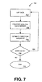
- FIG. 7 is an exemplary flow chart 700 of one method, among others, for determining the bearing angles of the detected object 20 or known object 504 , i.e., the angle between a local reference axis at the sensor node 18 and a ray extending from the sensor node towards the detected object, using the raw data collected by the sensor node 18 .
- the steps illustrated in FIG. 7 can be implemented in at least the sensor node or the COC 12 , or in a combination of both the sensor node and COC 12 .
- the flow chart shown in FIG. 7 is the detailed description of the step 406 in FIG. 4 that was mentioned in the previous paragraph.
- the sensor node 18 collects data. Typically, the sensor node 18 passively collects the data by detecting energy 27 emitted from the detected object 20 or known object 504 .
- step 704 data from each one of the sensors 28 in the sensor node 18 is processed.
- the processing includes, among other things, filtering and digitizing the data.
- the data can be processed at the sensor node or at the processing unit 26 .
- step 706 the data from all of the sensors 28 is used to determine the bearing angle of the object 20 ( 504 ) using techniques such as MVDR (Van Veen, B. D., and K. M. Buckley, “Beamforming: a versatile approach to spatial filtering,” IEEE ASSP Magazine, vol. 5, pp. 4-24, 1988) and/or a MUSIC (Adaptive Filter Theory by S. Haykin, published by Prentice Hall, 1991) which are well known techniques.
- MVDR Vehicle, B. D., and K. M. Buckley, “Beamforming: a versatile approach to spatial filtering,” IEEE ASSP Magazine, vol. 5, pp. 4-24, 1988
- MUSIC Adaptive Filter Theory by S. Haykin, published by Prentice Hall, 1991
- step 708 a determination is made as to whether there is more data, i.e., whether the sensors of the sensor node continue to detect the object or have detected another object. If there is more data, then the process returns to step 702 , otherwise, the process ends at step 710 .
- Step 408 in FIG. 4 pertains to recording the global position and time information of the object 20 ( 504 ) from GPS. More is said about this later.
- the final step 410 in FIG. 4 is where the coordinates of each sensor node 18 is determined. Detailed steps involved in step 410 of FIG. 4 are given in FIG. 8 .
- the process of determining the coordinates of the sensor node 18 has four major steps as listed below:
- step 804 for a set of data points from the sensor node, direction indicators or bearings of the object 20 ( 504 ) are calculated using well known and well documented techniques in the literature such as MVDR or MUSIC.
- the direction indicators are measured relative to a local reference axis. This local reference axis may be different from the global reference axis (normally global reference axis is true north).
- the offset between the two references is denoted by ‘ ⁇ ’.
- ⁇ i is the angle between a local reference axis and a ray extending from the sensor node towards the detected object and where the ⁇ 's are calculated using collected sensor node data using either MVDR or MUSIC or ally other angle estimator.
- Steps 802 and 806 are done essentially concurrently.
- the trajectory information of the object 504 which is traversing the neighborhood of the sensor node 18 , is collected.
- the trajectory information of the object 504 is provided to the COC 12 .
- trajectory information associates the position (the coordinates) of the object 504 at a given instance of time.
- the object's trajectory information is normally recorded every second or so and an object trajectory information data point comprises a time stamp and a given position, where the time stamp corresponds to when the object was located at the given position.
- the object's trajectory information is determined by a GPS system.
- the object's trajectory information is determined using other detectors that can determine the absolute or global position of the object 504 while the object 504 traverses the neighborhood of the sensor node.
- a subset of trajectory points of the object 504 is selected to be used in determining the sensor node 18 coordinates as some trajectory points result in more error in the sensor node coordinates than the other points.
- the source trajectory information data points are analyzed such that selected data points are used to determine the coordinates and orientation of the sensor node.
- the accuracy of the sensor node localization depends in part on the estimation accuracy of angles in the direction indicator.
- the direction indicator may change rapidly if the relative distance between the sensor node 18 and the object is small.
- ⁇ is approximately tell degrees (10°). Although an angle ⁇ of approximately ten degrees has been explicitly identified as an example, other angles are possible.
- the points at which the direction indicator angles change fast can be determined by computing the difference between the adjacent direction indicator angles estimated using sensor node data. Those points with a difference greater than ⁇ (10°) can be eliminated from the list of trajectory information data points used to calculate the sensor node coordinates.
- the coordinates of the sensor node are given in two dimensions. Consequently, the coordinates of the sensor node are initially calculated from the intersection of two circles. If the unknown coordinates of the sensor node were in three dimensions, then the unknown coordinates would be calculated from the intersection of three spheres.
- Estimation of the approximate coordinates of a sensor node 18 Initial estimation of the approximate coordinates of a sensor node 18 is done by first selecting three points on the trajectory of the object 504 and corresponding (same time stamps) bearing angles determined from the data collected at the sensor node 18 . Selection of the three points on the trajectory and the estimation of the approximate coordinates of the sensor node 18 is elaborated further.
- FIG. 9 illustrates a portion of a path 900 of a known object (not shown) and a sensor node 902 . Points on the path 900 are used to determine the coordinates of the sensor node 902 . Specifically, points 904 and 906 correspond to the position of the object at times t i and t j , respectively.
- Line 908 denotes the distance (d ij ) between the points 904 and 906 .
- object trajectory information data points are selected based upon angular separation ( ⁇ ) as measured at the sensor node and the distance between data points. Because the location of the sensor node is unknown, the distance (d ij ) between P i and P j is used as a parameter for selecting triangulation points. Generally, it is found that when the distance between P i and P j is greater than 300 meters a reasonable accuracy for the sensor node location is obtained.
- a first estimate of the coordinates of the sensor node is determined using object trajectory information data points and sensor node direction indicators.
- a sensor node 1002 is disposed at a location 1004 .
- Line 1006 represents the local reference axis, and the local reference axis 1006 is offset from a global reference axis 1008 by an amount epsilon ( ⁇ ).
- points 1010 , 1012 , and 1014 represent three object trajectory information data points, which are denoted by (x 1 , y 1 ; t 1 ), (x 2 , y 2 ; t 2 ), and (x 3 , y 3 ; t 3 ), respectively.
- FIG. 10A illustrates that the bearing angles 1016 included in the direction indicators are measured from the local reference axis 1006 of the sensor node 18 , and are denoted as ⁇ 1 , ⁇ 2 , and ⁇ 3 . These angles ⁇ 1 , ⁇ 2 , and ⁇ 3 correspond to the points 1010 , 1012 and 1014 of the trajectory of the object 504 respectively.
- Triangulation cannot be used to find the actual coordinates (X s , Y s ) of the sensor node 1002 because the orientation of the local reference axis 1006 is unknown. Consequently, the coordinates of position 1004 are determined using geometric and trigonometric relationships. So, instead of working with the angles ⁇ 1 , ⁇ 2 , and ⁇ 3 directly, work with the differences in angles, effectively nullifying the effect of orientation of the reference axis. Construct two circles with one of the intersection point giving the coordinates of the sensor node 18 using the differences in angles, and the known distances between the points 1010 , 1012 and 1014 . The description of construction of the two circles to determine the coordinates of the sensor node 18 follows.
- the circumference of the first circle 1018 includes points 1004 , 1010 , and 1012 .
- the circumference of the second circle 1022 includes points 1004 , 1012 , and 1014 .
- the coordinates of the center (C) and the radius (R) of each circle is determined using known quantities. Specifically, two known positions and the difference in the bearing angles ( ⁇ ) for those two known positions are used to determine each circle. Referring to FIG. 10B , a simple case of finding the coordinates of the center of a circle 1026 is illustrated.
- the two known positions 1028 and 1030 have coordinates (x 1 , y 1 ) and (x 2 , y 1 ), respectively, and are separated by a distance of d, d(x 2 ⁇ x 1 ).
- Point 1032 represents the midpoint of the line connecting positions 1028 and 1030 .
- the coordinates of point 1032 are (0.5(x 1 +x 2 ), y 1 ).
- the coordinates of the center C 1034 are (0.5(x 1 +x 2 ), y 1 +R cos( ⁇ )). It is a simple procedure to find the center of a circle or a sphere when the known points do not lie in the same horizontal plane.
- the intersection point (point 1004 ) of the circles 1018 and 1022 is calculated, and the calculated coordinates of the intersection point are regarded as the first estimated location of the sensor node 1002 .
- a first estimation of the offset angle ( ⁇ ) between the local reference axis 1006 and the global reference axis 1008 is determined.
- step 812 the coordinates of the sensor node are estimated using object trajectory information data and the sensor node direction indicators to triangulate upon the sensor node. Triangulation is now possible because a first approximation of the offset ( ⁇ ) between the local reference axis and the global reference axis has been calculated.
- the initial approximate estimate of the coordinates of the sensor node 18 is refined by averaging the estimates of the coordinates of the sensor node 18 using triangulation. The procedure is illustrated. Proper selection of points for triangulation results in minimizing triangulation errors.
- the position of a sensor node is denoted by S and P identifies the recorded object trajectory information data, i.e., P is a list of positions ⁇ P 1 , P 2 , . . . P N ⁇ at times ⁇ t 1 , t 2 , . . . t N ⁇ .
- the sensor node direction indictor or the estimate of the bearing angle given by MVDR/MUSIC is an estimate of angle ‘ ⁇ i ’, which is given by
- the ⁇ 's are translated into angles measured from the position of the object, as shown in FIG. 9 .
- the corresponding pair of angles ( ⁇ i , ⁇ j ) are used to estimate the location of the sensor.
- the initial estimate of the sensor location based upon triangulation is the mean value of the set S and is given by
- step 816 the object trajectory information and the sensor node data are synchronized such that the offset angle ( ⁇ ) between the local reference angle and the global reference angle is eliminated.
- the trajectory information of the object 504 consists of the position information along with the time stamps. These recorded time stamps are accurate to 1 sec. However, since the object 504 is moving the actual position information and the corresponding time stamps may be off by few milliseconds. Hence, synchronization of the bearing angles of the object trajectory points computed using the estimated sensor coordinates and the bearing angles determined from the data at sensor node 18 need to be synchronized in order to estimate the coordinates of the sensor node 18 . Moreover, there is propagation delay of the signals from the object 504 to the sensor node 18 . This delay depends on the separation distance between the sensor node 18 and the object 504 . This process of synchronization is presented here.
- ⁇ m ⁇ which are generated from the data of sensor node, are denoted as “luk_angls”. If there is a time offset between the two sets of data, then it is corrected such that they are synchronized while adjusting for the orientation of the sensor node.
- a coarse time delay in a number of seconds is determined.
- the following exemplary algorithm is then used to time synchronize the luk_angls with the hel_angls to a fraction of a second.
- the refinement of the sensor node location is done in iterations.
- weighted mean squared error instead of mean squared error is that the error in determining the angle of bearing ⁇ i increases with the distance between the sensor node 18 and the object 504 as the signal strength decreases, hence signal to noise ratio, with distance.
- the weights are selected so that they are inversely proportional to the distance.
- the new location that gives the minimum weighted mean squared error is declared as the new estimated location of the sensor node 18 .
- the process is repeated until the weighted mean squared error no longer decreases. The description of this process follows.
- step 820 the data is weighted and the mean square error between the sensor node bearing angles and the object bearing node angles is determined.
- the mean square error is calculated as follows:
- the weights are inversely proportional to the log of the distance between the estimated sensor node location and the known object positions.
- a calculation grid is established around the estimated sensor node coordinates.
- An example of such a calculation grid is identified in FIG. 11A with reference numeral 1100 .
- the calculation grid 1100 can be of arbitrary size.
- the calculation grid 1100 has one meter (m) increments and extends ten meters in both positive and negative directions for both the x-axis and y-axis from the estimated sensor node position, (X EST , Y EST ) 1102 . This generates a grid of 21 by 21 points ( 1104 ).
- the grid need not be square.
- the calculated error is incremented and stored as “old_error” and an iteration counter is set to zero, as indicated in step 824 .
- An iteration counter is used so that the process of refinement does not continue without bounds.
- step 826 the calculated error is compared with the stored old_error, and the iteration counter is compared to a maximum number of iterations. If the iteration count is greater than a maximum number of iterations, or if the old_error is less than the calculated error, then the process proceeds to step 836 and ends. In the first iteration, the conditions always fail and the procedure continues through steps 828 through 834 .
- step 828 the stored “old_error” is updated such that it is equal to the calculated error and the iterations counter is incremented.
- the error is calculated for every point 1104 in the defined calculation grid 1100 (see FIG. 11A ).
- the error can be calculated by actually considering a finer grid 1106 at each selected point 1104 , and computing the averaged weighted mean squared error of the finer grid. Computing the error at each point 1104 in this manner is not required, however, and one can ignore the finer grid 1106 , if desired. However, use of the liner grid 1106 increases the accuracy of the calculation.
- a new sensor location is established based on the minimum error as indicated in step 832 ; moreover, the minimum error is stored as the calculated error. Whichever point gives the minimum error is designated as estimated sensor location point (K,L).
- estimated sensor location point K,L
- step 834 we use this location to generate another coarse grid around it. The procedure then returns to step 826 .
Abstract
Description
-
- Use three points, whose coordinates are known (
FIG. 9 ), on the trajectory of the object 20 (504) and the corresponding bearing estimates from thesensor node 18 to estimate approximate location of thesensor node 18 using geometry (FIG. 10 ). - Use the approximate location of the
sensor node 18 estimated in the above step to compute the bearing angles of the object 20 (504) for each point on the trajectory with known coordinates using geometry. - Find the difference in the estimated bearing angles of the object 20 (504) in the previous step and the bearing angles of the object estimated from the data (for example, acoustic signals). Find the offset (ε) angle, that is, the difference between the global reference (usually true north) and the local reference of the
sensor node 18. - Adjust the location of the
sensor node 18 till the difference in bearing angles listed in the previous step is minimum. Last three steps are iterated till the difference in bearing angles can not be reduced any further (FIG. 11 ).
FIG. 8 is a detailed flow chart ofFIG. 4 , ofexemplary steps 800 for determining the location of a sensor node.Steps step 802, the sensor node collects data, i.e., the sensor node detects an object (object 504) as the object traverses the neighborhood of the sensor node. In some embodiments, the sensor node collects data over a time span and associates the time at which the sensor collected the data with the data. Typically, a sensor node data point is comprised of a time stamp and a period of collected data. Typically, the period is approximately one second or so.
- Use three points, whose coordinates are known (
where αi is measured with respect to the
βi=mod(180+γi,360), [Equation 2]
where ‘mod’ is the modulo operator.
d ij=√{square root over ((x i −x j)2+(y i −y j)2)}{square root over ((x i −x j)2+(y i −y j)2)}, [Equation 3]
where Pi=(xi, yi) and Pj=(xj, yj), respectively. Once the distance dij between two points on the trajectory and the angles βi and βj are determined, triangulation can be performed using the principles of trigonometry to find the location of the sensor node. Let P={Pi, Pj} represent the pairs of points such that the distance dij>300 meters. Note that Pi is the location of object at some instant of time ti in terms of casting and northing.
| offset_limit = 180; | ||
| max_s = 0; | ||
| for time_delay = −10: 1: 10, | ||
| hangls = delay “hel_angls” by the amount time_delay; | ||
| for offset_ang = − offset_limit : 1 : offset_limit | ||
| langls = mod(luk_angls + offset_ang, 360); | ||
| d = abs(langls − hangls); | ||
| s = num. of elements in d <= 5; | ||
| if s > max_s | ||
| orientation = offset_ang; | ||
| time_offset = time_delay; | ||
| luk_angls_new = langls; | ||
| hel_angls_new = hangls; | ||
| max _s = s; | ||
| end | ||
| end | ||
| end | ||
| luk_angls = luk_angls_new; | ||
| hel_angls = hel_angls_new; | ||
| max_s = 0; |
| n = num. of elements in luk_angls; |
| time_in_secs = 2:n-1; |
| for time_delay = −1: 0.1: 1, |
| x = time_in_secs + time_delay; |
| angls = interpolate luk_angls to provide values at new time given by ‘x’; |
| langls = mod(angls, 360); |
| d = abs(langls − hel_angls); |
| s = num. of elements in d <= 5; |
| if s > max_s |
| luk_angls_new = langls; |
| max _s = s; |
| end |
| end |
| luk_angls = luk_angls_new; |
for all i, where estimated coordinates of the
Generation of Weighted Mean Squared Error:
The error then given by
where ddi=di*wi−md.
Claims (17)
Priority Applications (1)
| Application Number | Priority Date | Filing Date | Title |
|---|---|---|---|
| US12/025,160 US8060338B2 (en) | 2005-03-31 | 2008-02-04 | Estimation of global position of a sensor node |
Applications Claiming Priority (2)
| Application Number | Priority Date | Filing Date | Title |
|---|---|---|---|
| US9414505A | 2005-03-31 | 2005-03-31 | |
| US12/025,160 US8060338B2 (en) | 2005-03-31 | 2008-02-04 | Estimation of global position of a sensor node |
Related Parent Applications (1)
| Application Number | Title | Priority Date | Filing Date |
|---|---|---|---|
| US9414505A Continuation-In-Part | 2005-03-31 | 2005-03-31 |
Publications (2)
| Publication Number | Publication Date |
|---|---|
| US20080228437A1 US20080228437A1 (en) | 2008-09-18 |
| US8060338B2 true US8060338B2 (en) | 2011-11-15 |
Family
ID=39763527
Family Applications (1)
| Application Number | Title | Priority Date | Filing Date |
|---|---|---|---|
| US12/025,160 Expired - Fee Related US8060338B2 (en) | 2005-03-31 | 2008-02-04 | Estimation of global position of a sensor node |
Country Status (1)
| Country | Link |
|---|---|
| US (1) | US8060338B2 (en) |
Cited By (1)
| Publication number | Priority date | Publication date | Assignee | Title |
|---|---|---|---|---|
| US20210088619A1 (en) * | 2014-07-22 | 2021-03-25 | Mitel Networks Corporation | Positioning System and Method |
Families Citing this family (10)
| Publication number | Priority date | Publication date | Assignee | Title |
|---|---|---|---|---|
| US7667646B2 (en) * | 2006-02-21 | 2010-02-23 | Nokia Corporation | System and methods for direction finding using a handheld device |
| US7629981B1 (en) * | 2006-11-03 | 2009-12-08 | Overwatch Systems Ltd. | System and method for using computer graphics techniques to gather histogram data |
| US8260324B2 (en) * | 2007-06-12 | 2012-09-04 | Nokia Corporation | Establishing wireless links via orientation |
| US8326324B2 (en) * | 2008-01-08 | 2012-12-04 | Wi-Lan, Inc. | Systems and methods for location positioning within radio access systems |
| US9279878B2 (en) | 2012-03-27 | 2016-03-08 | Microsoft Technology Licensing, Llc | Locating a mobile device |
| DE102012014397B4 (en) * | 2012-07-13 | 2016-05-19 | Audi Ag | Method for determining a position of a vehicle and vehicle |
| US9612121B2 (en) * | 2012-12-06 | 2017-04-04 | Microsoft Technology Licensing, Llc | Locating position within enclosure |
| WO2018027339A1 (en) | 2016-08-06 | 2018-02-15 | SZ DJI Technology Co., Ltd. | Copyright notice |
| CN109959921B (en) * | 2019-02-27 | 2021-03-26 | 浙江大学 | Acoustic signal distance estimation method based on Beidou time service |
| CN110996333A (en) * | 2019-11-06 | 2020-04-10 | 湖北工业大学 | Wireless sensor network node positioning method based on whale algorithm |
Citations (2)
| Publication number | Priority date | Publication date | Assignee | Title |
|---|---|---|---|---|
| US6392565B1 (en) * | 1999-09-10 | 2002-05-21 | Eworldtrack, Inc. | Automobile tracking and anti-theft system |
| US20050153786A1 (en) * | 2003-10-15 | 2005-07-14 | Dimitri Petrov | Method and apparatus for locating the trajectory of an object in motion |
-
2008
- 2008-02-04 US US12/025,160 patent/US8060338B2/en not_active Expired - Fee Related
Patent Citations (2)
| Publication number | Priority date | Publication date | Assignee | Title |
|---|---|---|---|---|
| US6392565B1 (en) * | 1999-09-10 | 2002-05-21 | Eworldtrack, Inc. | Automobile tracking and anti-theft system |
| US20050153786A1 (en) * | 2003-10-15 | 2005-07-14 | Dimitri Petrov | Method and apparatus for locating the trajectory of an object in motion |
Cited By (2)
| Publication number | Priority date | Publication date | Assignee | Title |
|---|---|---|---|---|
| US20210088619A1 (en) * | 2014-07-22 | 2021-03-25 | Mitel Networks Corporation | Positioning System and Method |
| US11852738B2 (en) * | 2014-07-22 | 2023-12-26 | Mitel Networks Corporation | Positioning system and method |
Also Published As
| Publication number | Publication date |
|---|---|
| US20080228437A1 (en) | 2008-09-18 |
Similar Documents
| Publication | Publication Date | Title |
|---|---|---|
| US8060338B2 (en) | Estimation of global position of a sensor node | |
| US10852388B2 (en) | Method and device for locating an electromagnetic emission source and system implementing such a method | |
| US6178141B1 (en) | Acoustic counter-sniper system | |
| CN102411142B (en) | Three-dimensional target tracking method and system, processor and software program product | |
| KR101221978B1 (en) | Localization method of multiple jammers based on tdoa method | |
| US20120182837A1 (en) | Systems and methods of locating weapon fire incidents using measurements/data from acoustic, optical, seismic, and/or other sensors | |
| CN108614268B (en) | Acoustic tracking method for low-altitude high-speed flying target | |
| US6727851B2 (en) | System for signal emitter location using rotational doppler measurement | |
| WO2005116682A1 (en) | An arrangement for accurate location of objects | |
| CN102004244B (en) | Doppler direct distance measurement method | |
| US20150260837A1 (en) | High precision radar to track aerial targets | |
| US11762085B2 (en) | Device, system and method for localization of a target in a scene | |
| CN103487798A (en) | Method for measuring height of phase array radar | |
| CN111308457A (en) | Method, system and storage medium for north finding of pulse Doppler radar | |
| Blumrich et al. | Medium-range localisation of aircraft via triangulation | |
| RU2275649C2 (en) | Method and passive radar for determination of location of radio-frequency radiation sources | |
| Grabbe et al. | Geo-location using direction finding angles | |
| US7388538B1 (en) | System and method for obtaining attitude from known sources of energy and angle measurements | |
| US20180231632A1 (en) | Multi-receiver geolocation using differential gps | |
| US11428802B2 (en) | Localization using particle filtering and image registration of radar against elevation datasets | |
| Burns et al. | IFSAR for the rapid terrain visualization demonstration | |
| CN115100243A (en) | Ground moving target detection and tracking method based on sequential SAR image | |
| US8138962B2 (en) | Method for processing measured vertical profiles of the power of the echoes returned following a transmission of radar signals | |
| Kirkko-Jaakkola et al. | Improving TTFF by two-satellite GNSS positioning | |
| RU2377594C1 (en) | Method of determining coordinates of object |
Legal Events
| Date | Code | Title | Description |
|---|---|---|---|
| AS | Assignment |
Owner name: UNITED STATES OF AMERICA AS REPRESENTED BY THE SEC Free format text: ASSIGNMENT OF ASSIGNORS INTEREST;ASSIGNOR:DAMARLA, THYAGARAJU;REEL/FRAME:020459/0159 Effective date: 20080204 |
|
| STCF | Information on status: patent grant |
Free format text: PATENTED CASE |
|
| FPAY | Fee payment |
Year of fee payment: 4 |
|
| FEPP | Fee payment procedure |
Free format text: MAINTENANCE FEE REMINDER MAILED (ORIGINAL EVENT CODE: REM.); ENTITY STATUS OF PATENT OWNER: LARGE ENTITY |
|
| LAPS | Lapse for failure to pay maintenance fees |
Free format text: PATENT EXPIRED FOR FAILURE TO PAY MAINTENANCE FEES (ORIGINAL EVENT CODE: EXP.); ENTITY STATUS OF PATENT OWNER: LARGE ENTITY |
|
| STCH | Information on status: patent discontinuation |
Free format text: PATENT EXPIRED DUE TO NONPAYMENT OF MAINTENANCE FEES UNDER 37 CFR 1.362 |
|
| FP | Lapsed due to failure to pay maintenance fee |
Effective date: 20191115 |