US7034697B2 - Awakening level estimation apparatus for a vehicle and method thereof - Google Patents
Awakening level estimation apparatus for a vehicle and method thereof Download PDFInfo
- Publication number
- US7034697B2 US7034697B2 US10/689,676 US68967603A US7034697B2 US 7034697 B2 US7034697 B2 US 7034697B2 US 68967603 A US68967603 A US 68967603A US 7034697 B2 US7034697 B2 US 7034697B2
- Authority
- US
- United States
- Prior art keywords
- value
- frequency component
- high frequency
- low frequency
- percentile value
- Prior art date
- Legal status (The legal status is an assumption and is not a legal conclusion. Google has not performed a legal analysis and makes no representation as to the accuracy of the status listed.)
- Active, expires
Links
Images
Classifications
-
- G—PHYSICS
- G08—SIGNALLING
- G08B—SIGNALLING OR CALLING SYSTEMS; ORDER TELEGRAPHS; ALARM SYSTEMS
- G08B21/00—Alarms responsive to a single specified undesired or abnormal condition and not otherwise provided for
- G08B21/02—Alarms for ensuring the safety of persons
- G08B21/06—Alarms for ensuring the safety of persons indicating a condition of sleep, e.g. anti-dozing alarms
Definitions
- the present invention relates to an awakening level estimation apparatus and an awakening level estimation method for vehicle, and particularly to a technique for estimating an awakening level of a driver by monitoring a displacement of a vehicle in a direction of vehicle width in a time series manner.
- An awakening level estimation technique capable of accurately deciding an awakening level even in case that a large change in travel environment or vehicle speed occurs is disclosed in a JP-A-2002-154345 which is prior application of an applicant of the present application.
- displacement amounts of a vehicle in a direction of vehicle width is first detected in a time series manner and each frequency component power is calculated by making frequency conversion of these displacement amounts.
- an average value of each of the frequency component powers is calculated as a high frequency component amount.
- a maximum value of the frequency component powers within a predetermined frequency domain including a stagger frequency to become apparent in a state in which an awakening level of a driver decreases is calculated as a low frequency component amount. Then, an awakening level of a driver is decided based on an evaluation value corresponding to a ratio of the high frequency component amount to the low frequency component amount.
- the awakening level of the driver is low in the case that the high frequency component amount is small and the low frequency component amount is large.
- the high frequency component amount is small
- the low frequency component amount is large.
- an accurate decision on the awakening level becomes difficult in the case that both of these component amounts are large (a driver with a large stagger) or the case that both of these component amounts are small (a driver with a small stagger).
- the present invention is implemented in view of such circumstances, and an object of the present invention is to decide an awakening level of a driver more accurately regardless of a personal difference among drivers.
- a first invention provides an awakening level estimation apparatus for vehicle.
- This estimation apparatus has a signal processing part for calculating each frequency component power by making frequency conversion of a displacement amount of a vehicle in a direction of vehicle width detected in a time series manner, a frequency component amount calculation part for calculating an average value of the frequency component powers calculated by the signal processing part as a high frequency component amount and also calculating a maximum value of the frequency component powers within a predetermined frequency domain including a stagger frequency to become apparent in a state in which an awakening level of a driver decreases as a low frequency component amount, a correction factor calculation part for calculating a high frequency percentile value in which the proportion of the total sum to the sum of incidences counted from the lower frequency component powers results in a predetermined proportion in a histogram of the high frequency component amount and calculating a low frequency percentile value in which the proportion of the total sum to the sum of incidences counted from the lower frequency component powers results in a predetermined proportion in a histogram of the low frequency percentile value in
- the predetermined proportion is preferably between about 70% and about 90%.
- the correction factor calculation part desirably calculates a first ratio between a predetermined normal high frequency percentile value corresponding to a high frequency percentile value of a normal driver and the calculated high frequency component percentile value and calculates a second ratio between a predetermined normal low frequency percentile value corresponding to a low frequency percentile value of a normal driver and the calculated low frequency component percentile value and calculates the correction factor based on the first ratio and the second ratio.
- the proportion of the normal low frequency percentile value to the normal high frequency percentile value is preferably between 2 times and 2.5 times.
- the evaluation value calculation part preferably calculates a ratio between the high frequency component amount and the low frequency component amount as the evaluation value in one of the case that the high frequency percentile value is larger than a predetermined upper limit value and the case that the high frequency percentile value is smaller than a predetermined lower limit value.
- the correction factor calculation part preferably calculates a correction low frequency percentile value by multiplying the low frequency percentile value by a ratio between the normal high frequency percentile value and the high frequency percentile value.
- the evaluation value calculation part desirably calculates a ratio between the high frequency component amount and the low frequency component amount as the evaluation value in one of the case that the correction low frequency percentile value is larger than a predetermined upper limit value and the case that the correction low frequency percentile value is smaller than a predetermined lower limit value.
- the frequency component power is preferably leveled by multiplying the frequency component power by a value multiplied by the frequency component power by a power number n of each frequency, and more specifically, the power number n is desirably a value of 2.0 or more to 3.0 or less.
- the evaluation value calculation part preferably calculates a high frequency component amount based on frequency component powers excluding a maximum value among the respective frequency component powers calculated by the frequency component amount calculation part.
- the evaluation value calculation part may calculate the evaluation value with time.
- the decision part preferably decides that it is in a situation in which a driver is to be warned in the case that a value of a counter is increased or decreased in response to the evaluation value and also the value of the counter reaches a determination value. Further, the decision part may vary the amount of change in the counter in response to the evaluation value.
- a second invention provides an awakening level estimation method for vehicle, the method for deciding an awakening level of a driver based on an evaluation value calculated.
- This estimation method has a first step of calculating each frequency component power by making frequency conversion of a displacement amount of a vehicle in a direction of vehicle width detected in a time series manner, a second step of calculating an average value of the frequency component powers calculated by a signal processing part as a high frequency component amount, a third step of calculating a maximum value of the frequency component powers within a predetermined frequency domain including a stagger frequency to become apparent in a state in which the awakening level of the driver decreases as a low frequency component amount, a fourth step of calculating a high frequency percentile value in which the proportion of the total sum to the sum of incidences counted from the lower frequency component powers results in a predetermined proportion in a histogram of the high frequency component amount, a fifth step of calculating a low frequency percentile value in which the proportion of the total sum to the sum of incidences counted from the lower frequency component
- the predetermined proportion is preferably between about 70% and about 90%.
- the sixth step may include a step of calculating a first ratio between a predetermined normal high frequency percentile value corresponding to a high frequency percentile value of a normal driver and the calculated high frequency component percentile value, a step of calculating a second ratio between a predetermined normal low frequency percentile value corresponding to a low frequency percentile value of a normal driver and the calculated low frequency component percentile value, and a step of calculating the correction factor based on the first ratio and the second ratio.
- the proportion of the normal low frequency percentile value to the normal high frequency percentile value is desirably between 2 times and 2.5 times.
- a ratio between the high frequency component amount and the low frequency component amount is preferably calculated as the evaluation value in one of the case that the high frequency percentile value is larger than a predetermined upper limit value and the case that the high frequency percentile value is smaller than a predetermined lower limit value.
- a correction low frequency percentile value may be calculated by multiplying the low frequency percentile value by a ratio between the normal high frequency percentile value and the high frequency percentile value.
- a ratio between the high frequency component amount and the low frequency component amount is preferably calculated as the evaluation value in one of the case that the correction low frequency percentile value is larger than a predetermined upper limit value and the case that the correction low frequency percentile value is smaller than a predetermined lower limit value.
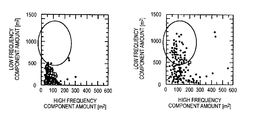
- FIGS. 1A and 1B are each a distribution characteristic diagram of frequency component amounts in a situation in which a driver with a small stagger is sleepy;
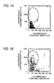
- FIGS. 2A and 2B are each a distribution characteristic diagram of frequency component amounts in a situation in which a driver with a large stagger is not sleepy;
- FIG. 3 is a block configuration diagram of an awakening level estimation apparatus
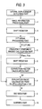
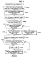
- FIG. 4 is a flowchart of an evaluation value calculation routine
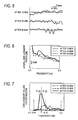
- FIG. 5 is a diagram showing a change in a lateral displacement amount with time
- FIG. 6 is a diagram showing each frequency component power
- FIG. 7 is an explanatory diagram of evaluation value calculation
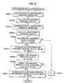
- FIG. 8 is a flowchart of a correction factor calculation routine
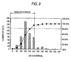
- FIG. 9 is an explanatory diagram of a high frequency percentile value
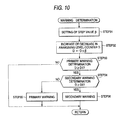
- FIG. 10 is a flowchart of a warning determination routine
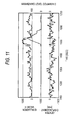
- FIG. 11 is a diagram showing an actual measured result at the time of freeway travel.
- FIGS. 1A and 1B are one example of a distribution characteristic diagram of frequency component amounts in a situation in which a driver with a small stagger is sleepy
- FIGS. 2A and 2B is one example of a distribution characteristic diagram of frequency component amounts in a situation in which a driver with a large stagger is not sleepy.
- the axis of abscissa shows a high frequency component amount
- the axis of ordinate shows a low frequency component amount.
- Black circle points shown in the drawing plot coordinate points (frequency component amount points) represented by high frequency component amounts calculated with certain timing and low frequency component amounts calculated with the same timing as this timing.
- the “frequency component amount” means discrete frequency component power obtained by making frequency conversion of a displacement amount of a vehicle in a direction of vehicle width detected in a time series manner. In a normal travel state, intentional steering caused by a curve etc. is performed, so that component amounts of the relatively high frequency side (high frequency component amounts) tend to stationarily appear over the whole of frequency domains regardless of an awakening state of a driver. In the embodiment, an average value of the frequency component powers calculated is used as the “high frequency component amount”.
- a maximum value of the frequency component powers within a predetermined frequency domain is used as the “low frequency component amount”.
- This frequency domain which is set with reference to a stagger frequency described below, is a low frequency band including a stagger frequency.
- An area surrounded by an ellipse is an area having a great influence on awakening level estimation, that is, an area in which the high frequency component amount is small and the low frequency component amount is large.
- the number of frequency component amount points present within the ellipse area increases as an awakening level of a driver decreases.
- a value obtained by dividing the low frequency component amount by the high frequency component amount (P′slp/P′ave described below) increases as the awakening level of the driver decreases.
- FIG. 1A shows a distribution characteristic in which the calculated frequency component amount points (high frequency component amounts, low frequency component amounts) are plotted as they are.
- the low frequency component amount is essentially small as compared with a characteristic of a normal driver. Because of that, there are cases where the frequency component amount points do not quite appear within the area surrounded by the ellipse even under travel in which an awakening level decreases. As a result of that, there is a possibility that it is wrongly determined that the awakening level does not decrease regardless of a state in which the awakening level decreases.
- FIG. 2A shows a distribution characteristic in which the calculated frequency component amount points (high frequency component amounts, low frequency component amounts) are plotted as they are.
- the low frequency component amount is essentially large as compared with a characteristic of a normal driver. Because of that, there are cases where many frequency component amount points appear within the area surrounded by the ellipse even under travel in which an awakening level does not decrease. As a result of that, there is a possibility that it is wrongly determined that the awakening level decreases regardless of a state in which the awakening level does not decrease.
- a cause of occurrence of the wrong determination in the two cases described above is the point that intrinsic characteristics of individual drivers about a stagger are not taken into account.
- the intrinsic characteristic of the driver is reflected on a low frequency percentile value and a high frequency percentile value.
- White square points shown in FIGS. 1 and 2 plot coordinate points (percentile points) represented by high frequency percentile values calculated with certain timing and low frequency percentile values calculated with the same timing as this timing.
- percentile points high frequency percentile values, low frequency percentile values
- frequency component amount points high frequency component amounts, low frequency component amounts
- the “high frequency percentile value” is a percentile value in which the proportion of the total sum to the sum of incidences counted from the lower frequency component powers results in a predetermined proportion in a histogram of the high frequency component amount.
- variations in the high frequency percentile value are relatively small and tend to become an approximately constant value (and hardly depend on an awakening state of the driver).
- the predetermined proportion is set to 80% and a 80 percentile value (80%ile value) is used, but this proportion is one example and may be within the range of between about 70% and about 90% (similar ratio applies to the next low frequency percentile value).
- the “low frequency percentile value” is a percentile value (for example, 80%ile value) in which the proportion of the total sum to the sum of incidences counted from the lower frequency component powers results in a predetermined proportion (for example, 80%) in a histogram of the low frequency component amount.
- This low frequency percentile value is different from the high frequency percentile value in characteristics, and variations are large and the variations tend to increase as an awakening level decreases.
- a ratio of the high frequency percentile value to the low frequency percentile value tends to become an approximately constant value as long as a driver is awake.
- a percentile point (a high frequency percentile value, a low frequency percentile value) of a normal driver (a virtual driver showing the travel characteristic with the highest incidence) was (200, 400 to 500).
- the high frequency percentile value of the normal driver is called “a normal high frequency percentile value” and is set to 200 in the embodiment.
- the low frequency percentile value of the normal driver is called “a normal low frequency percentile value” and is set to 500 in the embodiment.
- the percentile point of the normal driver is called “a normal percentile point”.
- the proportion of the normal low frequency percentile value to the normal high frequency percentile value may be within the range of between 2 times and 2.5 times and, for example, the normal percentile point may be set to (200, 400).
- the percentile points (high frequency percentile values, low frequency percentile values) concentrate in the vicinity of (100, 250). Therefore, in view of the fact that the percentile point of the normal driver is (200, 500), it can be decided that a driver with a characteristic shown in FIG. 1A is a driver with a small stagger essentially.
- the percentile points concentrate in (100 to 200, 400 to 600). Therefore, in view of the fact that the percentile point of the normal driver is (200, 500), it can be decided that a driver with a characteristic shown in FIG. 2A is a driver with a large stagger essentially.
- frequency component amount points are normalized by shifting the respective frequency component amount points by an aspect ratio between the percentile points and the normal percentile points calculated. For example, consider a certain frequency component amount point (100, 500) in FIG. 1 A. In this case, when it is assumed that a percentile point corresponding to this frequency component amount point is (100, 250), an aspect ratio between this and a normal percentile point (200, 500) results in (width 2.0 times, length 2.0 times). As a result of that, coordinates after the shift of this frequency component amount point result in (100 ⁇ 2.0, 500 ⁇ 2.0), namely (200, 1000). By performing such a shift with respect to all the frequency component amount points, a distribution characteristic shown in FIG. 1A is corrected to a distribution characteristic shown in FIG. 1 B. Through such a correction, many frequency component amount points appear within the area surrounded by the ellipse, so that a wrong determination about a driver with a small stagger essentially can be prevented effectively.
- a similar shift is performed with respect to a distribution characteristic shown in FIG. 2 A.
- a percentile point corresponding to this frequency component amount point is (100, 500)
- an aspect ratio between this and a normal percentile point (200, 500) results in (width 2.0 times, length 1.0 times).
- coordinates after the shift of this frequency component amount point result in (100 ⁇ 2.0, 1000 ⁇ 1.0), namely (200, 1000).
- the distribution characteristic shown in FIG. 2A is corrected to a distribution characteristic shown in FIG. 2 B. Through such a correction, the number of frequency component amount points appearing within the area surrounded by the ellipse decreases, so that a wrong determination about a driver with a large stagger essentially can be prevented effectively.
- the high frequency component amount and the low frequency component amount are corrected by the aspect ratio between the percentile point and the normal percentile point calculated.
- all the drivers can be handled in a manner similar to a normal driver regardless of a personal difference among drivers about a stagger. As a result of that, an awakening level of the driver can be decided more accurately.
- a lateral displacement detection part 1 detects a displacement (lateral displacement) of a vehicle in a direction of vehicle width.
- a monocular camera or a stereo camera using a CCD (charge-coupled device) etc. can be used in this detection part 1 .
- An image information processing part 2 processes an image obtained by the lateral displacement detection part 1 and finds a displacement amount of the vehicle. For example, images of right and left lanes of a road are picked up by the CCD and image data of one frame is stored in memory of the image information processing part 2 . Then, the right and left lanes are respectively recognized using an image recognition technique.
- an area corresponding to the lanes is identified by the image data of one frame using well-known recognition techniques such as stereo matching or a template about the lane.
- a vehicle position within the right and left lanes can be computed from, for example, a road width and a distance from the center of the vehicle in a lateral direction to the center of the right and left lanes.
- the lateral displacement detection part 1 can also detect the lateral displacement by combining a vehicle speed with a GPS and navigation system or communication between road vehicles based on a magnetic coil buried in a road in addition to a self-contained detection device such as a camera (see JP-A-9-99756 with respect to a stagger warning using navigation) Further, since the lateral displacement can be estimated by a steering angle, a steering angle sensor may be used as the lateral displacement detection part 1 . Also, the lateral displacement may be estimated by detecting a yaw rate or lateral acceleration. A lateral stagger (displacement amount) of the vehicle is measured, for example, with a resolution of 1 mm and a time step of 0.1 seconds. Data about the displacement amount is stored in a shift register 3 at any time. A sequence of displacement amount data calculated in a time series manner is stored by predetermined time. The data stored in the shift register 3 is sequentially updated with calculation and storage of new displacement amount data.
- a steering angle sensor may be used as the lateral displacement detection
- An FFT signal processing part 4 , a frequency component amount calculation part 5 , a correction factor calculation part 7 , an evaluation value calculation part 8 and a decision part 9 are functional blocks implemented by a general computer mainly comprising a CPU, RAM, ROM and an input/output circuit. Under control of an application for executing a routine described below, each member constructing the computer interacts and thereby the functional blocks 4 , 5 , 7 to 9 are implemented.
- an awakening level estimation program lower limit values allow, ⁇ 2 ′low and upper limit values ⁇ 1 high, ⁇ 2 ′high in a correction factor calculation routine, a normal value in correction factor calculation, a lower limit value Plow of a high frequency component amount P′ave, a table for setting of a step value ⁇ and warning determination values D 1 , D 2 , etc. are stored in the ROM.
- FIG. 4 is a flowchart of an evaluation value calculation routine and this routine is executed repeatedly at predetermined intervals.
- the FFT signal processing part 4 reads out displacement amount data for the past X seconds stored in the shift register 3 every Y seconds (for example, 90 seconds or shorter).
- Y seconds for example, 90 seconds or shorter.
- a long time for example, the order of 50 to 80 seconds
- the FFT signal processing part 4 makes frequency conversion of displacement amounts detected in a time series manner using a fast Fourier transformation (FFT) etc. and calculates each frequency component power (amplitude) P[i] in a frequency spectrum.
- FFT fast Fourier transformation
- 16 frequency component powers P[ 1 ] to P[ 16 ] are calculated in increments of 0.02 [Hz] in a frequency domain of 0.03 to 0.3 [Hz].
- the reason why a frequency domain lower than 0.03 Hz is not taken into account is because the power of its domain tends to increase at the time of curve travel and directly has nothing to do with an awakening level of a driver.
- the reason why a frequency domain higher than 0.3 Hz is not taken into account is because an operation amount necessary for calculation of an evaluation value H is decreased since the power within its frequency domain is generally small to a negligible extent.
- FIG. 5 is a diagram showing a relation between elapsed time from a driving start and a change in a lateral displacement amount.
- FIG. 6 is a diagram showing a relation between a frequency component i and its power P[i] by making frequency conversion of the displacement amount at each the elapsed time of FIG. 5 and is a diagram represented by connecting each of the discrete frequency component powers P[i] in a line graph manner.
- a dotted line shows each of the frequency component powers P[i] after about 10 minutes of travel and a broken line shows the powers P[i] after about 20 minutes and a solid line shows the powers P[i] after a lapse of about 50 minutes, respectively. From this diagram, it is found that there is a tendency in which the frequency component powers P[i] of a low frequency domain increase as travel time lengthens.
- FIG. 7 is a diagram showing a relation between the frequency components i and the leveled frequency component powers P′[i]. From distribution of the leveled frequency component powers P′[i], a general characteristic can be checked visually. From the same diagram, it is found that the power P′[ 4 ] of 0.09 [Hz] and the power P′[ 5 ] of 0.11 [Hz] in the vicinity of 0.1 [Hz] which is a low frequency domain, particularly a stagger frequency f 1 suddenly increase after about 50 minutes. In a state in which an awakening level of a driver decreases, the power in the vicinity of the stagger frequency f 1 tends to become apparent with respect to a lateral displacement of a vehicle.
- the awakening level of the driver can be decided by comparing the peak of the power in the vicinity of the stagger frequency f 1 with power states of frequency domains other than the stagger frequency.
- the stagger frequency f 1 means a frequency to become apparent (or converge) in the state in which the awakening level of the driver decreases (including a doze state).
- the stagger frequency tends to appear at about 0.08 to 0.12 [Hz] in a passenger vehicle, but is influenced by a response delay in vehicle behavior with steering operation, vehicle characteristics, a vehicle speed, etc. actually, so that a proper value is set every vehicle model through experiment or simulation.
- the stagger frequency f 1 is set to 0.01 [Hz].
- the frequency component amount calculation part 5 obtains the total sum of each of the frequency component powers P′[ 1 ] to P′[ 16 ] and calculates its average value as a high frequency component amount P′ave.
- the maximum power among each of the frequency component powers P′[ 1 ] to P′[ 16 ] is excluded and the high frequency component amount P′ave is calculated from the remaining frequency component powers P′[i]. The reason why such filtering is performed is because an influence of an increase in power of the stagger frequency f 1 and an influence of disturbance are eliminated.
- the frequency component amount calculation part 5 makes a determination of stagger frequency power, that is, compares sizes of the frequency component powers P′[ 4 ] and P′[ 5 ] in a predetermined frequency domain (0.09 to 0.11 [Hz]) including the stagger frequency f 1 (0.1 [Hz]). Then, the larger frequency component power is set as a low frequency component amount P′slp. That is, when the power P′[ 5 ] of 0.11 [Hz] is larger than the power P′[ 4 ] of 0.09 [Hz], the power P′[ 5 ] is set as the low frequency component amount P′slp (step 6 ).
- the power P′[ 4 ] of 0.09 [Hz] is larger than or equal to the power P′[ 5 ] of 0.11 [Hz]
- the power P′[ 4 ] is set as the low frequency component amount P′slp (step 7 ).
- a set of the high frequency component amount P′ave and the low frequency component amount P′slp calculated in steps 4 to 7 is stored in a shift register 6 .
- step 8 the correction factor calculation part 7 calculates a correction factor K 2 based on the high frequency component amount P′ave and the low frequency component amount P′slp.
- FIG. 8 is a flowchart of a correction factor calculation routine and this routine is executed repeatedly at predetermined intervals.
- the correction factor calculation part 7 acquires a history of the high frequency component amount P′ave stored in the shift register 6 .
- the number of histories of the high frequency component amount P′ave acquired is set to 500 samples as one example.
- the correction factor calculation part 7 calculates a high frequency percentile value ⁇ 1 based on the high frequency component amount P′ave.
- FIG. 9 is an explanatory diagram of the high frequency percentile value ⁇ 1 .
- the correction factor calculation part 7 creates a histogram of the high frequency component amount P′ave by the samples acquired.
- a value in which the proportion of the total sum to the sum of incidences counted from the lower frequency component powers results in a predetermined proportion is set to the high frequency percentile value ⁇ 1 .
- this proportion is set to 80% and a 80 percentile value of the high frequency component amount P′ave is calculated.
- the value ⁇ 1 calculated thus is a threshold value of 80% from the lower frequency component powers. By this threshold value, an abnormal value in the histogram is eliminated and a main data range in this histogram can be approximated to normal distribution.
- step 23 the correction factor calculation part 7 acquires a history of the low frequency component amount P′slp stored in the shift register 6 .
- the number of histories of the low frequency component amount P′slp acquired is set to 500 samples as one example.
- the correction factor calculation part 7 calculates a low frequency percentile value ⁇ 2 based on the low frequency component amount P′slp. First, the correction factor calculation part 7 creates a histogram of the low frequency component amount P′slp by the samples acquired. Next, in this histogram, it is counted from the lower frequency component powers and a 80 percentile value of the low frequency component amount P′slp is set to the low frequency percentile value ⁇ 2 .
- step 25 the correction factor calculation part 7 decides whether or not the high frequency percentile value ⁇ 1 is normal. That is, it decides whether or not this value ⁇ 1 is larger than a predetermined lower limit value ⁇ 1 low (for example, 100) or this value ⁇ 1 is larger than a predetermined upper limit value ⁇ 1 high (for example, 300).
- a predetermined lower limit value ⁇ 1 low for example, 100
- a predetermined upper limit value ⁇ 1 high for example, 300.
- the high frequency percentile value ⁇ 1 is smaller than the lower limit value ⁇ 1 low, when a correction is made to such a driver, there is a high possibility of wrongly determining that an awakening level decreases. Also, in the case that the high frequency percentile value ⁇ 1 is larger than the upper limit value ⁇ 1 high, there is a high possibility that a stagger of a vehicle occurs in a state in which the stagger is not recognized accurately or at the time of starting to enter a freeway.
- step 26 1 is set as the correction factor K 2 .
- this value is set to the evaluation value H as it is.
- step 27 the correction factor calculation part 7 calculates K 1 which is a ratio between the high frequency percentile value ⁇ 1 and a predetermined normal high frequency percentile value.
- This normal high frequency percentile value is a value corresponding to the high frequency percentile value ⁇ 1 of a normal driver and is set to 200 in the embodiment.
- step 28 the correction factor calculation part 7 calculates a correction low frequency percentile value ⁇ 2 ′ by multiplying the low frequency percentile value ⁇ 2 by the ratio K 1 calculated in step 27 .
- step 29 the correction factor calculation part 7 decides whether or not the correction low frequency percentile value ⁇ 2 ′ is normal. That is, it decides whether or not this value ⁇ 2 ′ is larger than a predetermined lower limit value ⁇ 2 ′low (for example, 400) or this value ⁇ 2 ′ is larger than a predetermined upper limit value ⁇ 2 ′high (for example, 500).
- a predetermined lower limit value ⁇ 2 ′low for example, 400
- this value ⁇ 2 ′ is larger than a predetermined upper limit value ⁇ 2 ′high (for example, 500).
- the flowchart proceeds to step 30 .
- the correction low frequency percentile value ⁇ 2 ′ is smaller than the lower limit value ⁇ 2 ′low, when a correction is made to such a driver, there is a high possibility of wrongly determining that an awakening level decreases. Also, in the case that the correction low frequency percentile value ⁇ 2 ′ is larger than the upper limit value ⁇ 2 ′high, it is in a state in which a decrease in an awakening level of a driver continues.
- step 26 1 is set as the correction factor K 2 .
- this value is set to the evaluation value H as it is in a manner similar to the case of step 26 .
- the correction factor calculation part 7 calculates the correction factor K 2 based on the correction low frequency percentile value ⁇ 2 ′.
- This correction factor K 2 is calculated as a ratio between the corrected low frequency percentile value ⁇ 2 ′ and a predetermined normal low frequency percentile value.
- This normal low frequency percentile value is a value corresponding to the low frequency percentile value ⁇ 2 of a normal driver and is set to 500 in the embodiment.
- the correction factor K 2 calculated thus is calculated by steps 25 to 30 in order to decide whether or not the high frequency percentile value ⁇ 1 and the correction low frequency percentile value ⁇ 2 ′ are normal.
- the value may be calculated by the following procedure. First, a first ratio which is a ratio between a normal high frequency percentile value and the high frequency percentile value ⁇ 1 is calculated. Next, a second ratio which is a ratio between a normal low frequency percentile value and the low frequency percentile value ⁇ 2 is calculated. Then, the correction factor K 2 can be calculated by totaling the first ratio and the second ratio calculated thus.
- step 9 the evaluation value calculation part 8 determines a lower limit of the high frequency component amount P′ave, that is, decides whether or not the high frequency component amount P′ave is smaller than a preset lower limit value Plow (for example, 100).
- a preset lower limit value Plow for example, 100.
- the high frequency component amount P′ave is smaller than the lower limit value Plow, it is decided that an awakening state of a driver is stable, and the high frequency component amount P′ave is set to the lower limit value Plow (step 10 ).
- step 10 is skipped and the flowchart proceeds to step 11 .
- the evaluation value calculation part 8 calculates the evaluation value H based on the following formula.
- This evaluation value H corresponds to an instantaneous awakening level without consideration of a factor with time, and is calculated by correcting a ratio between the high frequency component amount P′ave and the low frequency component amount P′slp by the correction factor K 2 .
- 1 is set to the correction factor K 2 in step 26 .
- the evaluation value H calculated in this case corresponds to an evaluation value H calculated without being corrected by the correction factor K 2 . Then, after the evaluation value H is calculated in step 11 , the present routine exits.
- the evaluation value H becomes a small value.
- the low frequency component amount P′slp P′[ 4 ] or P′[ 5 ]
- the evaluation value H results in a value reflecting the awakening level of the driver.
- FIG. 10 is a flowchart of a warning determination routine and this routine is executed repeatedly at predetermined intervals.
- the decision part 9 sets constants ⁇ 1 to ⁇ 8 , 0 as step values ⁇ from the following table based on the evaluation value H calculated in an evaluation value calculation routine which is another routine.
- these constants have a non-linear relation equipped with
- Evaluation value H Step value ⁇ >1000 + ⁇ 1 >900 + ⁇ 2 >800 + ⁇ 3 >500 + ⁇ 4 >400 + ⁇ 5 >300 ⁇ 0 >200 ⁇ 6 >100 ⁇ 7 >0 ⁇ 8
- step 32 the decision part 9 updates a value of the awakening level counter D by adding the step value ⁇ to the current value of the awakening level counter D or subtracting the step value ⁇ from the current value.
- step 33 a primary warning determination is made, that is, it is decided whether or not the awakening level counter D is larger than or equal to a first determination value D 1 . If not in this step 33 , it is decided that a driver is in an awakening state, and the present routine exits. On the other hand, when the awakening level counter D is larger than or equal to the first determination value D 1 , it is decided that there is a need to urge an awakening on the driver, and the flowchart proceeds to step 34 .
- a secondary warning determination is made, that is, it is decided whether or not the awakening level counter D is larger than or equal to a second determination value D 2 . If not in this step 34 , in order to give a warning of a stagger of a vehicle due to a decrease in an awakening level of a driver, the present routine exits after giving a primary warning to a warning part 10 (step 35 ). On the other hand, if so in step 34 , in order to give a warning of a doze state in which the awakening level of the driver decreases further, the present routine exits after giving secondary warning processing to the warning part 10 (step 36 ).
- the warning part 10 receives instructions from the decision part 9 and performs various warning processing for urging an awakening on the driver.
- various cases are considered and as one example, a case of sounding a collision warning is given. That is, when it is decided that the awakening level decreases, a warning distance between vehicles is set to a longish distance than usual (early timing).
- the warning part 10 may sound a deviation warning. For example, timing constructed so as to sound at the instant of treading on a lane is early set at the time of a decrease in the awakening level. Further, a doze warning may be sounded. For example, at the time of a decrease in the awakening level, “stagger caution” is displayed on a display screen along with a stagger warning beep.
- FIG. 11 is a diagram showing an actual measured result at the time of freeway travel, and the lower portion shows a characteristic of a lateral displacement of a vehicle and the upper portion shows a characteristic of the evaluation value H and the middle portion shows a characteristic of the awakening level counter D, respectively.
- the characteristic peaks continuously appear in the lateral displacement of the vehicle and the stagger frequency f 1 of 0.1 [Hz] becomes apparent.
- the evaluation value H increases and a value of the awakening level counter D is incremented, so that a warning to a driver is given properly.
- the peak of the evaluation value H singly appears even before a lapse of 1400 seconds.
- the warning to the driver is not given unless such peaks continuously appear (in other words, unless the awakening level counter D is continuously incremented).
- varying sizes of a value of the high frequency component amount P′ave and a value of the low frequency component amount P′slp caused by a personal difference among drivers can be solved by correcting the evaluation value H by the correction factor K 2 . Therefore, various drivers as shown in FIGS. 1 and 2 can be handled as a normal driver, so that a problem of a wrong determination caused by the personal difference among drivers can be solved and an awakening level of the driver can be decided more accurately.
- an awakening level of a driver is decided by comparing the peak of the power in the vicinity of the stagger frequency f 1 with the powers of frequency domains other than the stagger frequency. Therefore, there is no need to previously prepare samples at the time of normal driving and based on only data (including the just previous data) at the time of determination, the awakening level of the driver can be decided. As a result of that, without depending on a change in travel environment, the awakening level can be determined properly and a problem of a wrong determination caused by the change in travel environment as described in the conventional art can be solved.
- the evaluation value H is calculated after a lower limit value is set with respect to a level of the high frequency component amount P′ave described above.
- the peak of the power within a frequency domain including the stagger frequency f 1 becomes more apparent than that of the powers of frequency domains other than the stagger frequency due to a stagger of the lateral displacement of the vehicle, a decrease in the awakening level of the driver is detected.
- a detection technique even when a situation in which a lateral displacement amount is generally small or a slight side wind or a situation of passing by a large-size vehicle occurs at the time of stable high-speed travel, a wrong determination of the awakening level can be prevented.
Landscapes
- Business, Economics & Management (AREA)
- Emergency Management (AREA)
- Physics & Mathematics (AREA)
- General Physics & Mathematics (AREA)
- Traffic Control Systems (AREA)
- Emergency Alarm Devices (AREA)
- Auxiliary Drives, Propulsion Controls, And Safety Devices (AREA)
Abstract
Description
H=(P′slp×K 2)/P′ave×100
| Evaluation value H | Step value β | ||
| >1000 | +β1 | ||
| >900 | +β2 | ||
| >800 | +β3 | ||
| >500 | +β4 | ||
| >400 | +β5 | ||
| >300 | ±0 | ||
| >200 | −β6 | ||
| >100 | −β7 | ||
| >0 | −β8 | ||
Claims (26)
Applications Claiming Priority (2)
| Application Number | Priority Date | Filing Date | Title |
|---|---|---|---|
| JPP.2002-308086 | 2002-10-23 | ||
| JP2002308086A JP3997142B2 (en) | 2002-10-23 | 2002-10-23 | Awakening degree estimation device and awakening degree estimation method for vehicle |
Publications (2)
| Publication Number | Publication Date |
|---|---|
| US20040080422A1 US20040080422A1 (en) | 2004-04-29 |
| US7034697B2 true US7034697B2 (en) | 2006-04-25 |
Family
ID=32064330
Family Applications (1)
| Application Number | Title | Priority Date | Filing Date |
|---|---|---|---|
| US10/689,676 Active 2024-07-31 US7034697B2 (en) | 2002-10-23 | 2003-10-22 | Awakening level estimation apparatus for a vehicle and method thereof |
Country Status (4)
| Country | Link |
|---|---|
| US (1) | US7034697B2 (en) |
| EP (1) | EP1413469B1 (en) |
| JP (1) | JP3997142B2 (en) |
| DE (1) | DE60321637D1 (en) |
Cited By (5)
| Publication number | Priority date | Publication date | Assignee | Title |
|---|---|---|---|---|
| US20050126841A1 (en) * | 2003-12-10 | 2005-06-16 | Denso Corporation | Awakening degree determining system |
| US20080068186A1 (en) * | 2006-09-12 | 2008-03-20 | Zachary Thomas Bonefas | Method and system for detecting operator alertness |
| US20080068187A1 (en) * | 2006-09-12 | 2008-03-20 | Zachary Thomas Bonefas | Method and system for detecting operator alertness |
| US20090033501A1 (en) * | 2007-07-31 | 2009-02-05 | National Taiwan University Of Science And Technology | Online monitoring method of driver state and system using the same |
| EP2824644A1 (en) | 2013-07-09 | 2015-01-14 | Wincor Nixdorf International GmbH | Till system provided with a monitor screen that can be used on both sides |
Families Citing this family (11)
| Publication number | Priority date | Publication date | Assignee | Title |
|---|---|---|---|---|
| JP4316962B2 (en) * | 2003-08-26 | 2009-08-19 | 富士重工業株式会社 | Driver's alertness estimation device and alertness estimation method |
| JP4366145B2 (en) * | 2003-08-26 | 2009-11-18 | 富士重工業株式会社 | Driver's alertness estimation device and alertness estimation method |
| US20050205331A1 (en) * | 2004-03-17 | 2005-09-22 | Mr. Polchai Phanumphai | Automatic Driver's Aide |
| JP4182131B2 (en) * | 2007-03-13 | 2008-11-19 | トヨタ自動車株式会社 | Arousal level determination device and arousal level determination method |
| JP4748122B2 (en) * | 2007-06-28 | 2011-08-17 | 日産自動車株式会社 | Lane departure prevention device |
| US20110320163A1 (en) * | 2008-11-06 | 2011-12-29 | Volvo Technology Corporation | Method and system for determining road data |
| FR2954745B1 (en) * | 2009-12-30 | 2012-01-06 | Continental Automotive France | METHOD FOR DETERMINING A PARAMETER REPRESENTATIVE OF THE VIGILANCE STATUS OF A VEHICLE DRIVER |
| JP5423724B2 (en) * | 2011-04-28 | 2014-02-19 | トヨタ自動車株式会社 | Driver status determination device |
| JP5967196B2 (en) * | 2012-05-23 | 2016-08-10 | トヨタ自動車株式会社 | Driver state determination device and driver state determination method |
| JP6331875B2 (en) * | 2014-08-22 | 2018-05-30 | 株式会社デンソー | In-vehicle control device |
| CN113450595A (en) * | 2021-06-30 | 2021-09-28 | 江西昌河汽车有限责任公司 | Human-vehicle interaction anti-collision early warning system and early warning method |
Citations (7)
| Publication number | Priority date | Publication date | Assignee | Title |
|---|---|---|---|---|
| US5786765A (en) * | 1996-04-12 | 1998-07-28 | Mitsubishi Jidosha Kogyo Kabushiki Kaisha | Apparatus for estimating the drowsiness level of a vehicle driver |
| US5798695A (en) | 1997-04-02 | 1998-08-25 | Northrop Grumman Corporation | Impaired operator detection and warning system employing analysis of operator control actions |
| US5815070A (en) | 1995-08-01 | 1998-09-29 | Honda Giken Kogyo Kabushiki Kaisha | Driving state-monitoring apparatus for automotive vehicles |
| EP0999520A2 (en) | 1998-10-16 | 2000-05-10 | Fuji Jukogyo Kabushiki Kaisha | Driver's arousal level estimating apparatus for vehicle and method of estimating arousal level |
| US6097295A (en) * | 1998-01-28 | 2000-08-01 | Daimlerchrysler Ag | Apparatus for determining the alertness of a driver |
| JP2002087107A (en) | 2000-09-14 | 2002-03-26 | Denso Corp | Running condition detector, awakening degree detector, awakening degree corresponding control device, and recording medium |
| EP1209019A2 (en) | 2000-11-24 | 2002-05-29 | Fuji Jukogyo Kabushiki Kaisha | Driver's arousal level estimating apparatus for vehicle and method of estimating arousal level |
-
2002
- 2002-10-23 JP JP2002308086A patent/JP3997142B2/en not_active Expired - Fee Related
-
2003
- 2003-10-22 US US10/689,676 patent/US7034697B2/en active Active
- 2003-10-23 EP EP03024477A patent/EP1413469B1/en not_active Expired - Fee Related
- 2003-10-23 DE DE60321637T patent/DE60321637D1/en not_active Expired - Lifetime
Patent Citations (7)
| Publication number | Priority date | Publication date | Assignee | Title |
|---|---|---|---|---|
| US5815070A (en) | 1995-08-01 | 1998-09-29 | Honda Giken Kogyo Kabushiki Kaisha | Driving state-monitoring apparatus for automotive vehicles |
| US5786765A (en) * | 1996-04-12 | 1998-07-28 | Mitsubishi Jidosha Kogyo Kabushiki Kaisha | Apparatus for estimating the drowsiness level of a vehicle driver |
| US5798695A (en) | 1997-04-02 | 1998-08-25 | Northrop Grumman Corporation | Impaired operator detection and warning system employing analysis of operator control actions |
| US6097295A (en) * | 1998-01-28 | 2000-08-01 | Daimlerchrysler Ag | Apparatus for determining the alertness of a driver |
| EP0999520A2 (en) | 1998-10-16 | 2000-05-10 | Fuji Jukogyo Kabushiki Kaisha | Driver's arousal level estimating apparatus for vehicle and method of estimating arousal level |
| JP2002087107A (en) | 2000-09-14 | 2002-03-26 | Denso Corp | Running condition detector, awakening degree detector, awakening degree corresponding control device, and recording medium |
| EP1209019A2 (en) | 2000-11-24 | 2002-05-29 | Fuji Jukogyo Kabushiki Kaisha | Driver's arousal level estimating apparatus for vehicle and method of estimating arousal level |
Cited By (12)
| Publication number | Priority date | Publication date | Assignee | Title |
|---|---|---|---|---|
| US20050126841A1 (en) * | 2003-12-10 | 2005-06-16 | Denso Corporation | Awakening degree determining system |
| US7222690B2 (en) * | 2003-12-10 | 2007-05-29 | Denso Corporation | Awakening degree determining system |
| US20080068186A1 (en) * | 2006-09-12 | 2008-03-20 | Zachary Thomas Bonefas | Method and system for detecting operator alertness |
| US20080068187A1 (en) * | 2006-09-12 | 2008-03-20 | Zachary Thomas Bonefas | Method and system for detecting operator alertness |
| US20080068184A1 (en) * | 2006-09-12 | 2008-03-20 | Zachary Thomas Bonefas | Method and system for detecting operator alertness |
| US20080068185A1 (en) * | 2006-09-12 | 2008-03-20 | Zachary Thomas Bonefas | Method and System For Detecting Operator Alertness |
| US7692548B2 (en) * | 2006-09-12 | 2010-04-06 | Deere & Company | Method and system for detecting operator alertness |
| US7692550B2 (en) * | 2006-09-12 | 2010-04-06 | Deere & Company | Method and system for detecting operator alertness |
| US7692549B2 (en) * | 2006-09-12 | 2010-04-06 | Deere & Company | Method and system for detecting operator alertness |
| US7692551B2 (en) * | 2006-09-12 | 2010-04-06 | Deere & Company | Method and system for detecting operator alertness |
| US20090033501A1 (en) * | 2007-07-31 | 2009-02-05 | National Taiwan University Of Science And Technology | Online monitoring method of driver state and system using the same |
| EP2824644A1 (en) | 2013-07-09 | 2015-01-14 | Wincor Nixdorf International GmbH | Till system provided with a monitor screen that can be used on both sides |
Also Published As
| Publication number | Publication date |
|---|---|
| DE60321637D1 (en) | 2008-07-31 |
| EP1413469B1 (en) | 2008-06-18 |
| US20040080422A1 (en) | 2004-04-29 |
| EP1413469A3 (en) | 2005-02-09 |
| JP2004145508A (en) | 2004-05-20 |
| EP1413469A2 (en) | 2004-04-28 |
| JP3997142B2 (en) | 2007-10-24 |
Similar Documents
| Publication | Publication Date | Title |
|---|---|---|
| US7034697B2 (en) | Awakening level estimation apparatus for a vehicle and method thereof | |
| US6686845B2 (en) | Driver's arousal level estimating apparatus for vehicle and method of estimating arousal level | |
| EP1510396B1 (en) | Wakefulness estimating apparatus and method | |
| EP1510395B1 (en) | Wakefulness estimating apparatus and method | |
| CN111942389B (en) | Driving assistance system, lane change determination unit and lane change determination method | |
| US8229643B2 (en) | Acceleration control system | |
| JP2001167397A (en) | Driving situation monitoring device for vehicle | |
| JP3061459B2 (en) | Driver abnormal steering judgment device | |
| JP4529394B2 (en) | Driver's vehicle driving characteristic estimation device | |
| JP2004220348A (en) | Vehicle running condition detection system and vehicle running control device | |
| JP3400092B2 (en) | Vehicle travel path estimation device | |
| EP0999520B1 (en) | Driver's arousal level estimating apparatus for vehicle and method of estimating arousal level | |
| JP3319201B2 (en) | Inattentive driving judgment device | |
| JPH079880A (en) | Abnormality warning device for driver | |
| WO2013168209A1 (en) | Meander determination device | |
| JP3901035B2 (en) | Vehicle information providing device | |
| JP3492963B2 (en) | Vehicle driving condition monitoring device | |
| JP2869927B2 (en) | Vehicle driving condition monitoring device | |
| JP2856049B2 (en) | Drowsy driving detection device | |
| JP4924524B2 (en) | Driver state estimation device | |
| KR19990084339A (en) | Lane Object Recognition | |
| JPH08220225A (en) | Inter-vehicle distance detecting device |
Legal Events
| Date | Code | Title | Description |
|---|---|---|---|
| AS | Assignment |
Owner name: FUJI JUKOGYO KABUSHIKI KAISHA, JAPAN Free format text: ASSIGNMENT OF ASSIGNORS INTEREST;ASSIGNOR:OYAMA, HAJIME;REEL/FRAME:014637/0983 Effective date: 20031017 |
|
| FEPP | Fee payment procedure |
Free format text: PAYOR NUMBER ASSIGNED (ORIGINAL EVENT CODE: ASPN); ENTITY STATUS OF PATENT OWNER: LARGE ENTITY |
|
| STCF | Information on status: patent grant |
Free format text: PATENTED CASE |
|
| FPAY | Fee payment |
Year of fee payment: 4 |
|
| FPAY | Fee payment |
Year of fee payment: 8 |
|
| AS | Assignment |
Owner name: FUJI JUKOGYO KABUSHIKI KAISHA, JAPAN Free format text: CHANGE OF ADDRESS;ASSIGNOR:FUJI JUKOGYO KABUSHIKI KAISHA;REEL/FRAME:033989/0220 Effective date: 20140818 |
|
| AS | Assignment |
Owner name: SUBARU CORPORATION, JAPAN Free format text: CHANGE OF NAME;ASSIGNOR:FUJI JUKOGYO KABUSHIKI KAISHA;REEL/FRAME:042624/0886 Effective date: 20170401 |
|
| MAFP | Maintenance fee payment |
Free format text: PAYMENT OF MAINTENANCE FEE, 12TH YEAR, LARGE ENTITY (ORIGINAL EVENT CODE: M1553) Year of fee payment: 12 |