JP2009520306A - Parallel multirate circuit simulation - Google Patents
Parallel multirate circuit simulation Download PDFInfo
- Publication number
- JP2009520306A JP2009520306A JP2008547473A JP2008547473A JP2009520306A JP 2009520306 A JP2009520306 A JP 2009520306A JP 2008547473 A JP2008547473 A JP 2008547473A JP 2008547473 A JP2008547473 A JP 2008547473A JP 2009520306 A JP2009520306 A JP 2009520306A
- Authority
- JP
- Japan
- Prior art keywords
- matrix
- circuit
- preconditioned
- instructions
- splitting
- Prior art date
- Legal status (The legal status is an assumption and is not a legal conclusion. Google has not performed a legal analysis and makes no representation as to the accuracy of the status listed.)
- Granted
Links
Images
Classifications
-
- G—PHYSICS
- G06—COMPUTING; CALCULATING OR COUNTING
- G06F—ELECTRIC DIGITAL DATA PROCESSING
- G06F30/00—Computer-aided design [CAD]
- G06F30/30—Circuit design
- G06F30/36—Circuit design at the analogue level
- G06F30/367—Design verification, e.g. using simulation, simulation program with integrated circuit emphasis [SPICE], direct methods or relaxation methods
Landscapes
- Engineering & Computer Science (AREA)
- Computer Hardware Design (AREA)
- Physics & Mathematics (AREA)
- Theoretical Computer Science (AREA)
- Microelectronics & Electronic Packaging (AREA)
- Evolutionary Computation (AREA)
- Geometry (AREA)
- General Engineering & Computer Science (AREA)
- General Physics & Mathematics (AREA)
- Management, Administration, Business Operations System, And Electronic Commerce (AREA)
- Complex Calculations (AREA)
Abstract
回路シミュレーションにおいて並列方程式を解くためのコンピュータ実装された方法を説明する。この方法は、回路ヤコビ行列を疎結合のパーティションに分割するステップと、電圧ベクトルと行列をパーティションにしたがってリオーダーするステップと、ヤコビ行列を二つの行列MとNにスプリットするステップとを含み、Mは並列処理に適した行列であり、Nは結合行列である。MとNは、M−1Jx=(I+M−1N)x=M−1rを形成するようにプレコンディションされ、ヤコビ行列Jは反復解法を用いて解かれる。
【選択図】図4A computer implemented method for solving parallel equations in circuit simulation is described. The method includes dividing the circuit Jacobian matrix into loosely coupled partitions, reordering the voltage vector and matrix according to the partition, and splitting the Jacobian matrix into two matrices M and N, Is a matrix suitable for parallel processing, and N is a coupling matrix. M and N are preconditioned to form M −1 Jx = (I + M −1 N) x = M −1 r, and the Jacobian matrix J is solved using an iterative solution.
[Selection] Figure 4
Description
電子設計自動化(EDA)では、集積回路設計者が自分の設計を探求し、検証するために利用することができるソフトウェアが開発されている。半導体産業がナノメートルの時代に入ったため、設計者はEDAツールを使って、製造される回路にナノメートルレベルの影響があるかどうかを調べることが必要になってきている。設計を検証しなかったとしたら、製造される集積回路は高い確率で機能不全に陥り、再設計を余儀なくされ、費用がかかる。 In Electronic Design Automation (EDA), software has been developed that can be used by integrated circuit designers to explore and verify their designs. As the semiconductor industry has entered the nanometer era, designers need to use EDA tools to determine if the circuits being manufactured have nanometer-level effects. If the design was not verified, the integrated circuit produced would malfunction with a high probability and would have to be redesigned and expensive.
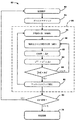
回路シミュレーションは回路設計が動作するかどうかを検証する最も正確な方法である。図1は、初期設計が実現されたときから回路を製造する際に行われる典型的な変換を例示するフローダイアグラム50である。ブロック52は初期回路設計を示す。この設計は、一連の接続されたデバイスエレメント54に分解される。当該設計における各デバイスエレメントは、半導体製造工場や製造者によって検証されてきた正確な解析的モデルでモデル化される。解析的なモデルで表されたデバイスエレメントを用いれば、波線で示すブロック55で示される回路シミュレータが、電圧値や電流値をある期間にわたってシミュレートすることができる。回路シミュレータ55は、データに対して回路シミュレーションの演算を行うようにプログラムされたコンピュータシステムを含む。回路シミュレーションにおいて、当該回路のすべてのノードの電圧値と電流値は、フローダイアグラム50のブロック56に表された微分代数方程式(DAE)の系(システム)を解くことにより得られる。
Circuit simulation is the most accurate way to verify whether a circuit design works. FIG. 1 is a flow diagram 50 illustrating a typical transformation that occurs in manufacturing a circuit from when the initial design is realized.
DAEは有限差分法を用いて離散化することができ、ニュートン−ラフソン法のような非線形反復法を用いて、反復処理で方程式を解く。各反復において、非線形方程式が以前に得られた解の周りで線形化され、ブロック58で示される線形化された方程式系が生成される。そして、この線形系を解く必要がある。
DAE can be discretized using a finite difference method, and an equation is solved by an iterative process using a nonlinear iterative method such as Newton-Raphson method. At each iteration, the nonlinear equations are linearized around the previously obtained solution to produce a linearized system of equations, indicated by
行列解法技術が多くの科学、工学の分野で広く用いられている。EDAにおいて、行列解法技術は、回路シミュレーションのような分野で線形方程式系を解く上で欠かすことができない。 Matrix solving techniques are widely used in many scientific and engineering fields. In EDA, matrix solution technology is indispensable for solving linear equation systems in fields such as circuit simulation.
回路方程式は次のような形を取る。 The circuit equation takes the form:

ここでvは当該回路でシミュレートされるすべてのノードにおける電圧のベクトルである。Q(v)はこれらのノードにおける電荷である。i(v)はこれらのノードにおける電流である。u0は当該回路の電源である。 Where v is a vector of voltages at all nodes simulated by the circuit. Q (v) is the charge at these nodes. i (v) is the current at these nodes. u 0 is the power supply of the circuit.
上記の方程式を解く際、有限微分法を用いて最初に微分演算子を近似する。ここでは説明のため、後退オイラー法を説明するが、他の有限微分法が使われているならば、他の方法を同様に適用することができる。離散方程式系は次のような形になる。 When solving the above equation, the finite differentiation method is first used to approximate the differential operator. Here, for the sake of explanation, the backward Euler method will be described, but if other finite differentiation methods are used, other methods can be applied as well. The discrete equation system has the form
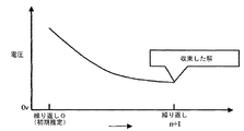
ここで時間ステップtmは既知であると仮定し、時刻tm+1における解を求める。非線形離散方程式を解くためにニュートン−ラフソン反復法を用いることができる。反復処理において、初期の推定値v0が与えられる。その後、解v1、v2、…のシーケンスが得られ、図2のグラフに示されるような非線形方程式の解に収束する。各反復において、非線形方程式は、以前の反復で得られた既知の解vnの周りに線形化される。そして、次の線形方程式系を解いてΔvを得る。 Here, it is assumed that the time step t m is known, and a solution at the time t m + 1 is obtained. Newton-Raphson iteration can be used to solve nonlinear discrete equations. In an iterative process, an initial estimate v 0 is given. Thereafter, a sequence of solutions v 1 , v 2 ,... Is obtained and converges to a solution of a nonlinear equation as shown in the graph of FIG. In each iteration, the nonlinear equations are linearized around the known solutions v n obtained in the previous iteration. Then, Δv is obtained by solving the following linear equation system.
ここで here
Δvを求めた後、更新された解vn+1=vn+Δvを求める。このプロセスは次の条件が満たされるまで続く。 After obtaining Δv, an updated solution v n + 1 = v n + Δv is obtained. This process continues until the following conditions are met:
ここでtolはある小さな誤差許容値である。式4の条件が満たされると、解は図2に示すように収束したと考えられ、tm+1における解は次のようになる。 Here, tol is a small error tolerance. When the condition of Equation 4 is satisfied, the solution is considered to have converged as shown in FIG. 2, and the solution at t m + 1 is as follows.
従来のSpice回路シミュレーションにおいて、誤差チェックはすべてのノードに対して行われ、|Δv|は、ベクトルΔvすなわち全ノードにおける解の変化の中で、すべてのエントリの内の最大絶対値である。式4が満たされると、手続きは1タイムステップ進み、フローチャート50のブロック56に戻り、次の時間に対応する次の非線形方程式系を解く。このようにして、モデル化された回路において過渡的な変動をシミュレートすることができる。
In conventional Spice circuit simulation, error checking is performed for all nodes, and | Δv | is the maximum absolute value of all entries in the vector Δv, ie, the change in solution at all nodes. When equation 4 is satisfied, the procedure advances one time step and returns to
各時刻において生成された電圧値を解析し、回路シミュレーションが当該回路の期待された演算と合致しているかどうかどうかを判定する。たとえば、電圧値は回路設計の論理的な解析と比較される。別の例では、電圧値と電流値は、回路設計の電源およびタイミングの分析を実行するために使うことができる。演算68において、シミュレーションが期待された演算に合致しないならば、設計が変更され、欠陥が正される。そして、手続きは新しい回路設計のもとで演算52に戻る。しかし、電圧が期待された演算と比べて遜色がないならば、回路設計はプロトタイプとして製造される。すなわち、製造回路70が生成される。
The voltage value generated at each time is analyzed to determine whether the circuit simulation is consistent with the expected operation of the circuit. For example, the voltage value is compared with a logical analysis of the circuit design. In another example, voltage and current values can be used to perform power and timing analysis of the circuit design. In
線形系を解くことの主要な部分は、回路ヤコブ行列を解くことであり、これは、LU分解ステップと従来の直接的アプローチにおける前向きおよび後ろ向き代入ステップとを含む。高速で正確な行列解法は、高速で正確な回路シミュレーションにおいてたいへん重要である。 The main part of solving the linear system is to solve the circuit Jacob matrix, which includes the LU decomposition step and the forward and backward substitution steps in the conventional direct approach. Fast and accurate matrix solving is very important in fast and accurate circuit simulation.
行列解法技術は二つのカテゴリに分けることができる。一つのカテゴリは直接行列解法と呼ばれる。他方のカテゴリは反復行列解法と呼ばれる。 Matrix solving techniques can be divided into two categories. One category is called direct matrix solving. The other category is called iterative matrix solution.
回路シミュレーションにおいて次の線形系を考える。 Consider the following linear system in circuit simulation.
![]()
![]()
ここでJは回路のヤコビ行列であり、rは残差ベクトルであり、Δvはノード電圧解の更新ベクトルである。 Here, J is a Jacobian matrix of the circuit, r is a residual vector, and Δv is an update vector of the node voltage solution.
直接行列解法は、行列Jを最初にLU分解する The direct matrix solving method first LU decomposes matrix J
![]()
![]()
ここでLは下三角行列であり、Uは上三角行列である。その後、次式を解き、線形系に対する解Δvを得る。 Here, L is a lower triangular matrix and U is an upper triangular matrix. Thereafter, the following equation is solved to obtain a solution Δv for the linear system.
![]()
![]()
かつ And
以下の説明において、便宜上、Δvを表すためにxを用いる。 In the following description, for convenience, x is used to represent Δv.
反復行列解法は、反復しながら解を得るか、解に近づこうとする。初期推定値x0のもとで、反復法は次の処理で解xに近づく。 The iterative matrix method tries to obtain or approach a solution while iterating. Under the initial estimate x 0 , the iterative method approaches the solution x in the next process.
ここでn≧0であり、Bは反復解法のためにプレコンディション(precondition)された行列である。反復解法が効率的であるためには、この処理は、相対的に小さい反復回数で許容できる正確さで解に近づくことができるものでなければならず、Bxnの計算は高速でなければならない。Krylov部分空間反復法は十分な収束特性をもち、合理的な速さで回路解に近づくことができる。プレコンディションの目的は、反復処理を高速化するために、行列Bを恒等行列に近づけることである。 Here, n ≧ 0 and B is a preconditioned matrix for iterative solution. For iterative solution to be efficient, this process must be one that can approach the solution with an accuracy acceptable by relatively small number of iterations, the calculation of Bx n must be fast . The Krylov subspace iteration method has sufficient convergence properties and can approach the circuit solution at a reasonable speed. The purpose of preconditioning is to bring matrix B closer to the identity matrix in order to speed up the iterative process.
回路シミュレーションにおいて、線形系のサイズは非常に大きくなり、行列の要素のパターンが疎(スパース)になることがある。このため、標準的な回路シミュレータは、行列Aの疎(スパース)行列表現を採用する。行列の疎(スパース)表現では、非零である行列の要素だけを保存するのが一般的である。疎(スパース)行列の非零パターンはLU分解の効率化のために重要である。これは、オペレーションはLおよびUに非零のエントリを生成することがある一方、同じ場所のJのエントリはゼロであるからである。これらのエントリはフィル−イン(fill-in)と呼ばれる。フィルインの数を減らすため、線形系をリオーダー(reorder)することができる。リオーダーリングの処理は線形系においてベクトルxとbのパーミュテーション(入れ替え)である。 In circuit simulation, the size of a linear system may become very large, and the pattern of matrix elements may become sparse. For this reason, a standard circuit simulator employs a sparse matrix representation of the matrix A. In a sparse representation of a matrix, it is common to preserve only non-zero matrix elements. A non-zero pattern of a sparse matrix is important for improving the efficiency of LU decomposition. This is because the operation may generate non-zero entries in L and U, while the J entry in the same place is zero. These entries are called fill-in. To reduce the number of fill-ins, the linear system can be reordered. The reordering process is permutation (replacement) of vectors x and b in a linear system.
![]()
![]()
ここでJrはJの行と列をパーミュテーション/リオーダーリングしたものであり、r’はrの行パーミュテーションであり、x’はxの列パーミュテーションである。さらなる例示の便宜のために、下付文字および上付文字は今後の説明では省略する。リオーダーリングの目的は、行列のLU分解の過程で生成されるフィル−インの数を最小にすることであり、これによりシミュレーションが高速化する。 Here J r is obtained by permutation / reordering the rows and columns of J, r 'is a row permutation of r, x' is a column permutation of x. For further illustrative convenience, subscripts and superscripts will be omitted in the following description. The purpose of reordering is to minimize the number of fill-ins generated during the process of LU decomposition of the matrix, which speeds up the simulation.
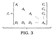
典型的な並列回路シミュレーションにおいて、このタイプのリオーダーリングは別の目的で実行される。回路行列を図3に示すいわゆるダブルボーダー(double-bordered)系にリオーダーしたいとする。 In a typical parallel circuit simulation, this type of reordering is performed for another purpose. Suppose we want to reorder the circuit matrix to the so-called double-bordered system shown in FIG.
リオーダーされた行列JrのLU分解を実行するにあたって、あるブロックオペレーションは並列に実行することができる。すなわち、行列ブロックA1、A2、…、Am−1のLU分解は並列に実行できる。並列計算のボトルネックは、最後のブロックのLU分解を実行することである。結合(カップリング)ブロック、すなわちCブロックやDブロックからの寄与があるため、最後のブロックはLU分解処理の過程で密になりうることに留意する。 In executing LU decomposition of reordered matrix J r, certain block operations can be executed in parallel. That is, the LU decomposition of the matrix blocks A 1 , A 2 ,..., A m−1 can be executed in parallel. The bottleneck of parallel computing is to perform LU decomposition of the last block. Note that the last block can become dense during the LU decomposition process due to contributions from the coupling (coupling) blocks, ie C and D blocks.
Y.Saadらによって提案されたドメインベース・マルチレベル再帰ブロック不完全LU法(BILUTM)は我々の方法とは異なる。BILUTMは一般的な行列解法をとして提案された。その方法の一つのアプローチは、Krylov部分空間法をBILUTMのすべてのレベルで適用することであり、BILUTM法の出版物で報告されている。その手続きのl番目のレベルで、行列のブロック因数分解が次のように近似的に計算される(上付文字はレベル番号に対応する)。 Y. The domain-based multilevel recursive block incomplete LU method (BILUTM) proposed by Saad et al. Is different from our method. BILUTM was proposed as a general matrix solution. One approach to that method is to apply the Krylov subspace method at all levels of BILUTM, as reported in the BILUTM method publications. At the l-th level of the procedure, the block factorization of the matrix is approximately calculated as follows (superscript corresponds to the level number):
ここで
回路シミュレーションにとって、上記のアプローチを取ると、トップ回路行列レベルでKrylov部分空間反復法を適用することになる。これは、特別な特徴をもつ回路シミュレーション行列の性質のゆえに非常に非効率的である。より具体的には、回路シミュレーション行列は、非常に大きいが、疎であるかもしれない。Krylov部分空間法をトップレベルで適用することは、Krylov部分空間ベクトルがトップレベル行列と同じサイズであることを意味する。これらのベクトルは大きなコンピュータメモリを消費し、計算が遅くなる。BILUMの別の修正した使い方は、BILUTMの特定レベル、すなわち特定の縮小(reduced)ブロックでKrylov部分空間法を適用することである。しかし、トップレベル行列を縮小ブロックに減らしたとしても、縮小ブロックは近似技術を適用しなければ、非常に密になることがある。 For circuit simulation, taking the above approach would apply the Krylov subspace iteration method at the top circuit matrix level. This is very inefficient due to the nature of the circuit simulation matrix with special features. More specifically, the circuit simulation matrix may be very large but sparse. Applying the Krylov subspace method at the top level means that the Krylov subspace vector is the same size as the top level matrix. These vectors consume large computer memory and are slow to compute. Another modified usage of BILUM is to apply the Krylov subspace method at a specific level of BILUTM, ie a specific reduced block. However, even if the top-level matrix is reduced to reduced blocks, the reduced blocks can become very dense if no approximation technique is applied.
Saadらによるアプローチにおいて、不完全LU分解(ILU)は保存される一方、近似誤差は破棄される。これは、ILU分解をプレコンディション行列として用いるには良い。よって、各反復において、元の行列とベクトルの積、およびプレコンディション行列とベクトルの積を計算することが必要である。 In the approach by Saad et al., Incomplete LU decomposition (ILU) is preserved while approximation errors are discarded. This is good for using ILU decomposition as a precondition matrix. Thus, at each iteration, it is necessary to calculate the product of the original matrix and the vector and the product of the precondition matrix and the vector.
上述の理由のため、直接・反復ハイブリッドアプローチが、並列計算を用いたときのLU分解によってもたらされるボトルネックの問題を解決するために必要である。特に回路シミュレータ55(図1)が、複数のプロセッサコアまたはプロセッサユニットをもつコンピュータシステムであり、ロジックに応答してコンピュータシステムに回路シミュレーションの機能を実行させるものである場合、新しいハイブリッドアプローチが必要である。このロジックはソフトウェア、ハードウェア、もしくはソフトウェアとハードウェアの組み合わせによって実装することができる。 For the reasons described above, a direct and iterative hybrid approach is necessary to solve the bottleneck problem caused by LU decomposition when using parallel computing. In particular, if the circuit simulator 55 (FIG. 1) is a computer system having a plurality of processor cores or processor units and causes the computer system to perform circuit simulation functions in response to logic, a new hybrid approach is required. is there. This logic can be implemented in software, hardware, or a combination of software and hardware.
大まかに言えば、本発明は、並列マルチレート回路シミュレータを提供し、直接法と反復法の両方の利点を組み合わせ、シミュレーション過程で並列性を増やすことで上記のニーズに応えるものである。 Broadly speaking, the present invention provides a parallel multi-rate circuit simulator that meets the needs described above by combining the advantages of both direct and iterative methods and increasing parallelism during the simulation process.
本発明は、プロセス、装置、システム、デバイス、方法を含め、数多くのやり方で実装することができることが理解されよう。本発明のいくつかの実施の形態を以下で説明する。 It will be appreciated that the present invention can be implemented in numerous ways, including processes, apparatus, systems, devices, methods. Several embodiments of the present invention are described below.
ある実施の形態では、回路シミュレーションにおいて並列方程式を解くためのコンピュータで実装された方法が記述される。この方法は、回路ヤコビ行列を疎結合のパーティションに分割し、このパーティションにしたがって電圧ベクトルと当該行列をリオーダーリングし、当該ヤコビ行列を二つの行列MとNに分ける。ここでMは並列処理に適した行列であり、Nは結合行列である。MとNはその後、M−1Jx=(I+M−1N)x=M−1rとなるようにプレコンディションされ、ヤコビ行列Jが反復解法を使って解かれる。 In one embodiment, a computer-implemented method for solving parallel equations in circuit simulation is described. This method divides the circuit Jacobian matrix into loosely coupled partitions, reorders the voltage vector and the matrix according to the partition, and divides the Jacobian matrix into two matrices M and N. Here, M is a matrix suitable for parallel processing, and N is a coupling matrix. M and N are then preconditioned so that M −1 Jx = (I + M −1 N) x = M −1 r, and the Jacobian matrix J is solved using an iterative solution.
本発明の利点は、これから述べる詳細な説明において、図面を用いながら発明の原理を例示することによって明らかになる。 The advantages of the present invention will become apparent from the following detailed description, by way of example illustrating the principles of the invention using the drawings.
本発明は、これから述べる詳細な説明において、同じような構成要素には同様の符号を付した図面を参照することにより、容易に理解される。 The present invention will be readily understood by referring to the drawings in which like reference numerals refer to like elements in the detailed description that follows.
これから述べる説明において、本発明を完全に理解するために、数多くの具体的な詳細が説明される。しかし、本発明はそのような具体的な詳細がなくても実施できることは当業者にとって明らかである。別の例では、周知の処理操作や実装の詳細については詳細には述べられていない。いたずらに発明をわかりにくくすることを避けるためである。 In the following description, numerous specific details are set forth in order to provide a thorough understanding of the present invention. However, it will be apparent to those skilled in the art that the present invention may be practiced without such specific details. In other instances, well known processing operations and implementation details have not been described in detail. This is to avoid unnecessarily obscuring the invention.
プロトタイプ回路の生成に先立ち、当該回路をモデル化するための公知の技術を用いて微分代数方程式(DAE)の系を生成してもよい。DAEを数値評価に適したものにするために離散化する。離散化の方法としていろいろな方法が知られており、DAEの系を離散化するためにいずれの方法を用いてもよい。DAEが非線形である場合、たとえば回路がトランジスタのような非線形の構成要素を用いているなどの場合、線形系になるように線形化し、ここで説明する並列行列法を用いて解くことができるようにしてもよい。線形系に対する解は、回路の各ノードにおいて、電圧、電流および/または電荷を与えるものであるか、電圧、電流および/または電荷に対する変化を与えるものであってもよい。最終的な解を解析することで、物理試験のためにプロトタイプを生成するのに先立って、モデル化された回路が期待通りに振る舞うかどうかを確かめることができる。 Prior to the generation of the prototype circuit, a system of differential algebraic equations (DAE) may be generated using known techniques for modeling the circuit. Discretize DAE to make it suitable for numerical evaluation. Various methods are known as discretization methods, and any method may be used to discretize a DAE system. When the DAE is nonlinear, for example, when the circuit uses a nonlinear component such as a transistor, the DAE is linearized to be a linear system and can be solved using the parallel matrix method described here. It may be. The solution for the linear system may provide a voltage, current and / or charge at each node of the circuit, or provide a change to the voltage, current and / or charge. Analyzing the final solution can verify that the modeled circuit behaves as expected prior to generating a prototype for physical testing.
[パーティショニングおよびスプリッティング] [Partitioning and splitting]
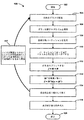
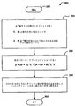
図4は、回路シミュレーションのために並列方程式を高速に解くための実施の形態に係る方法を提示するフローチャート100である。ここで説明する本アプローチは、節点解析、修正節点解析、分散エレメントを用いた方程式などを含む異なる定式化の回路方程式に適用することができる。この手続きは開始ブロック102で始まり、オペレーション104に進み、行列がグラフで表現される。最初、回路ヤコビ行列は疎結合ブロックに分割される。行列Jは、一般的な並列マルチレベルグラフ分割(パーティショニング)アルゴリズムを適用することができるようにグラフに変換される。この変換において、まず対称行列が以下のように得られる。
FIG. 4 is a
ここでJ’はJの転置行列であり、1≦i,j≦Jsizeである。JsizeはJのサイズである。 Here, J ′ is a transpose matrix of J, and 1 ≦ i and j ≦ J size . J size is the size of J.
Jsは次のようにしてグラフに変換される。エッジが下三角または上三角部分の各エントリに対して生成される。行i、列jのエントリはグラフにおいてはi番目の頂点とj番目の頂点を結ぶエッジとして表される。各頂点は同じインデックスの行や列を表す。その後、並列グラフ分割アルゴリズムを適用して、グラフを負荷分散したコンポーネントに分割し、そのコンポーネントを分離するためにカットするのに必要なエッジの数を最小化する。適切な並列グラフ分割アルゴリズムが知られており、すぐに利用可能である。分割の後、すべての結合エントリはスプリットされ、グラフのエッジは、最後のブロックにリオーダーされるというよりはむしろ、第2の行列にカットされることになる。 J s is converted into a graph as follows. An edge is generated for each entry in the lower or upper triangular part. The entry of row i and column j is represented as an edge connecting the i-th vertex and the j-th vertex in the graph. Each vertex represents a row or column with the same index. A parallel graph partitioning algorithm is then applied to divide the graph into load-distributed components and minimize the number of edges required to cut to separate the components. Suitable parallel graph partitioning algorithms are known and are readily available. After splitting, all join entries will be split and the edges of the graph will be cut into a second matrix rather than being reordered to the last block.
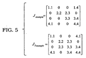
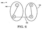
このプロセスは図5および図6の例で説明される。図5において、Jexampleは行列の例であり、JSexampleはJexampleを対称行列に変換したものである。JSexampleは図6に示すようにグラフ150に変換することができる。図4に戻り、手続きはオペレーション106および107に続き、グラフ分割アルゴリズムがオペレーション104で生成されたグラフに適用され、オペレーション108に示すように負荷分散されたパーティションが生成される。図5の例で言えば、結果的に得られるグラフ150は図6に示される。グラフ150は二つのパーティション152と154に分割され、ただ一つのエッジ156だけがカットのために必要である。
This process is illustrated in the examples of FIGS. In FIG. 5, J example is an example of a matrix, and J Example is obtained by converting J example into a symmetric matrix. J Example can be converted into a
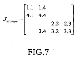
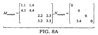
次に、オペレーション110において、行列Jexampleは、対応するグラフパーティションにしたがって、図7に示されるようにリオーダーされる。この例では、第2パーティション(2,3)は第1パーティション(1,4)のノードの後、リオーダーされる。パーティショニング(分割)の後、行列はオペレーション112において二つのマトリックスにスプリットされる。説明の目的のため、スプリッティングを次のように標記する。
Next, in
![]()
![]()
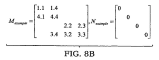
ここでMは並列計算のために適した行列であり、Nは結合行列である。たとえば、行列をスプリットする方法として、図8Aおよび8Bに示すような二通りの方法がある。 Here, M is a matrix suitable for parallel calculation, and N is a coupling matrix. For example, there are two methods for splitting a matrix as shown in FIGS. 8A and 8B.
オペレーション114において、線形系をプレコンディションし、反復法を適用して次のように行列Jを解いてもよい。
In
![]()
![]()
ここでx≡Δvであり、Iは対角成分が1で非対角成分が0である恒等行列である。 Here, x≡Δv, and I is an identity matrix having a diagonal component of 1 and an off-diagonal component of 0.
プレコンディショニングの目的は、プレコンディションされた行列I+M−1Nをできる限り恒等行列に近づけることである。このようにして、反復法が近似解に収束するまでの反復ステップが少なくなる。従来のFastMOS回路シミュレータは、パーティショニングのヒューリスティクスをたくさん用いて、弱い結合(カップリング)すなわちMOSFETデバイスのゲートにおける容量結合を生成する。こういったヒューリスティクスは依然としてここでも有用である。しかし、FastMOS回路シミュレータで使われる従来の緩和タイプの方法よりもずっと先進的な反復法を適用することができる。ここで説明する先進的な反復法は強い結合を扱うこともできる。こういった反復法の収束特性は、行列Nに現れる強い結合に対しても依然として十分有効である。 The purpose of preconditioning is to make the preconditioned matrix I + M −1 N as close as possible to the identity matrix. In this way, iterative steps are reduced until the iterative method converges to an approximate solution. Conventional FastMOS circuit simulators use a lot of partitioning heuristics to create weak coupling, or capacitive coupling at the gate of a MOSFET device. Such heuristics are still useful here. However, iterative methods that are much more advanced than the conventional relaxation type methods used in FastMOS circuit simulators can be applied. The advanced iterative method described here can also handle strong coupling. Such convergence characteristics of the iterative method are still sufficiently effective for strong coupling appearing in the matrix N.
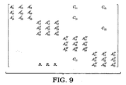
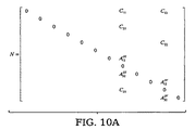
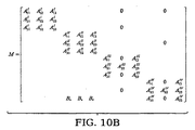
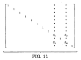
並列計算の性能を改善するため、分割されリオーダーされた行列は、まず上非対角ブロックのエントリを見つけることでスプリットしてもよい。たとえば、行列がブロック分割の後、図9に示す構造をもつと仮定する。見つかった上非対角ブロックはC11、C21、C12およびC22である。これらは行列の二つの列、列8と列11に属している。図10Aおよび図10Bに示すように、列8と列11のエントリは対角エントリを除いてすべて、結合行列Nに移動することができる。行列のスプリットの後、直接行列解法において行列操作M−1Nを適用してもよい。M−1Nには二つだけ列があることに留意されたい。行列I+M−1Nは図11に示された形を取る。 To improve the performance of parallel computing, the split and reordered matrix may be split by first finding the entry of the upper off-diagonal block. For example, assume that the matrix has the structure shown in FIG. 9 after block partitioning. The upper off-diagonal blocks found are C 11 , C 21 , C 12 and C 22 . These belong to the two columns of the matrix, column 8 and column 11. As shown in FIGS. 10A and 10B, all entries in columns 8 and 11 can be moved to the coupling matrix N except for diagonal entries. After the matrix split, the matrix operation M −1 N may be applied in the direct matrix solution. Note that there are only two columns for M −1 N. The matrix I + M −1 N takes the form shown in FIG.
図4に戻り、オペレーション112で行列をスプリッティングし、オペレーション114でプレコンディショニングした後、独立した部分系がオペレーション116によって次のように与えられ、解かれる。
Returning to FIG. 4, after splitting the matrix at
オペレーション116において、この系は結合系に縮小され、解かれる。系のサイズに依存して、あるいは、行列の特性解析を通して、系が直接解法によって効率的に解くことができるかどうかに依存して、オペレーション117に示されるように、オペレーション104から116は、再帰的にさらに部分系を縮小するために繰り返される。この再帰は図12および図15を参照して以下でさらに説明する。オペレーション118において、縮小された結合系の解が方程式15に後ろ向き代入され、当該手続きは完了ブロック120に示すように終了する。このように、後ろ向き代入を使って、すべての残りの解を得ることができる。結合インデックスの集合は次のように表記される。
In
![]()
![]()
このアプローチは結合部分系のサイズが比較的小さいときに有効である。結合部分系のサイズが大きいときは効果が薄れる。結合部分系の行列は次のように密である。 This approach is effective when the size of the coupled subsystem is relatively small. The effect diminishes when the size of the coupled subsystem is large. The matrix of coupled subsystems is dense as follows:
行列Sのサイズが大きいならば、その逆行列を求めるのは効率的ではない。 If the size of the matrix S is large, it is not efficient to obtain the inverse matrix.
並列計算において、方程式18の行列Sがボトルネックとなり、並列行列解法のスケーラビリティをより多くのCPUコアあるいは多くの結合をもつ系に制限してしまう。理想的には、パーティションの数はCPUコアの数に比例し、パーティションが多いと、N行列により多くのエントリが生じる。 In parallel computation, the matrix S of Equation 18 becomes a bottleneck, limiting the scalability of the parallel matrix solution to a system with more CPU cores or more connections. Ideally, the number of partitions is proportional to the number of CPU cores, and more partitions result in more entries in the N matrix.
[直接・反復ハイブリッド法] [Direct / iterative hybrid method]
図12は、行列I+M−1Nを解くための直接・反復ハイブリッドあるいは組み合わせ法の手続きの例を示すフローチャート200である。この手続きは開始ブロック202で示すように始まり、オペレーション204に進み、M−1がU−1L−1に置き換えられる。次に、オペレーション206において、U−1L−1Nが次のように3つの部分にスプリットされる。
FIG. 12 is a
最初の部分Eは、U−1L−1Nの計算の後、比較的大きな値になる行列のエントリを取る。第2の部分(LU)−1F1と第3の部分U−1F2は計算過程で、比較的小さな値を取る。 The first part E takes a matrix entry that is relatively large after the calculation of U −1 L −1 N. The second part (LU) −1 F 1 and the third part U −1 F 2 take relatively small values in the calculation process.
F1は次式の計算過程で、形成される。 F 1 is formed in the calculation process of the following equation.
![]()
![]()
F2は次式の計算過程で、形成される。 F 2 is formed in the calculation process of the following equation.
![]()
![]()
F1とF2を前向き消去L−1と後ろ向き代入U−1の過程でスプリットアウトする際、フィル−インエントリの相対的な大きさがチェックされる。もしそのエントリが元のベクトルにあるなら、それはF1またはF2にスプリットアウトされることはない。その代わり、異なる大きさの許容値を用いて結合部分系の行や他の行のエントリを制御してもよい。 When splitting out F 1 and F 2 in the process of forward erasure L −1 and backward substitution U −1 , the relative size of the fill-in entry is checked. If the entry is in the original vector, it is not to be split out to F 1 or F 2. Instead, differently sized tolerances may be used to control the rows of the connected subsystem and other row entries.
上記のアプローチはSaadらのアプローチとは異なる。このアプローチでは不完全なLU分解の残余は保たれるが、Saadのアプローチでは不完全なLU分解の残余は破棄される。それは「背景」の節で前に説明した通りである。 The above approach is different from the approach of Saad et al. This approach preserves the incomplete LU decomposition residue, but the Saad approach discards the incomplete LU decomposition residue. It is as explained earlier in the “Background” section.
上記のようにU−1L−1Nを3つの部分にスプリットすると、M−1は次を与える。 Splitting U −1 L −1 N into three parts as described above gives M −1 as follows:
![]()
![]()
この系には独立の結合部分系があることに留意すべきである。部分系の行および列のインデックスは結合インデックス集合ICに属する。行列I+Eの部分系への射影は次のように表記できる。 It should be noted that there are independent coupled subsystems in this system. Subsystem row and column indexes belong to the combined index set I C. The projection of the matrix I + E onto the subsystem can be expressed as follows.
![]()
![]()
オペレーション208において、この行列は、以下のように方程式22の部分系へのプレコンディショナー(preconditioner)として使われる。
In
![]()
![]()
最後に、オペレーション210において、Krylov部分空間反復法を適用することができる。たとえば、一般最小残余(GMRES)法を用いてプレコンディションされた系を解くことができる。
Finally, in
ここで述べるKrylov部分空間ベクトルの長さは縮小された部分系のサイズのことであるが、Saadの方法ではKrylov部分空間ベクトルの長さは元の行列のサイズのことであり、それは「背景」の節で前に説明した通りである。 The length of the Krylov subspace vector described here is the size of the reduced subsystem, but in the Saad method, the length of the Krylov subspace vector is the size of the original matrix, which is the “background” As described in the previous section.
縮小された部分系を解くために直接解法を用いることは都合がよいことを留意すべきである。それは、縮小された系が非常に疎であるときに意味がある。こうすることにより、その方法は純粋な直接法になる。非常に疎な行列に対して、直接解法は反復解法よりも高速になりうる。ある実施の形態では、この柔軟性を今から述べる直接・反復ハイブリッド法に有効に組み入れている。 It should be noted that it is convenient to use a direct solution to solve the reduced subsystem. It makes sense when the reduced system is very sparse. This makes the method a pure direct method. For very sparse matrices, the direct solution can be faster than the iterative solution. In some embodiments, this flexibility is effectively incorporated into the direct and iterative hybrid method now described.
部分系に対する解が得られた後、部分系にその解を後ろ向き代入することを通して全体の系に対する解が得られ、この手続きは完了ブロック212で示すように終了する。
After the solution for the subsystem is obtained, the solution for the entire system is obtained by backwardly assigning the solution to the subsystem, and the procedure ends as indicated by
縮小された部分系(I+E)|Sを解くために上記の直接・反復ハイブリッド法を再帰的に適用してもよいことに留意する。各再帰ステップにおいて、縮小された部分系のサイズはさらに小さくなる。ある実施の形態では、縮小された部分系のサイズが予め定めた閾値よりも小さくなったとき、あるいは、部分系が行列特性解析を通じて直接解法にとって効率的であると判定されたとき、再帰は停止する。この時点で直接法は、最終的な小さな部分系に適用され、この手続きは完了ブロック212で示されるように終了する。たとえば、ある実施の形態では、直説法は、部分系の行列が100行以下になったときに適用される。別の実施の形態では、直説法は、部分系の行列のLU分解が生成するフィル−インの数が小さくなったときに適用される。
Note that the direct and iterative hybrid method described above may be applied recursively to solve the reduced subsystem (I + E) | S. At each recursion step, the size of the reduced subsystem is further reduced. In some embodiments, recursion stops when the size of the reduced subsystem becomes less than a predetermined threshold or when the subsystem is determined to be efficient for direct solution through matrix characterization. To do. At this point, the direct method is applied to the final small subsystem, and the procedure ends as indicated by
[最小頂点セパレータを用いた行列のリオーダーリング] [Reordering matrix using minimum vertex separator]
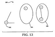
別の例示的な実施の形態では、回路行列が頂点セパレータの集合にしたがってリオーダーされ、より効率的な解法技術が適用される。頂点セパレータの集合は、グラフを二つの連結されていないコンポーネントすなわちサブグラフに分けるために、当該グラフから取り除くことができる頂点の集合であり、Sに接続するエッジを伴う。このグラフ分割アルゴリズムは頂点セパレータの最小集合を見つけることを試みる。たとえば、頂点セパレータの最小集合は図6のグラフ150の例では一つの頂点であり、図13に示すように頂点4である。頂点3を頂点セパレータとして選ぶこともできる。
In another exemplary embodiment, the circuit matrix is reordered according to a set of vertex separators and a more efficient solution technique is applied. A set of vertex separators is a set of vertices that can be removed from the graph to divide the graph into two unconnected components or subgraphs, with edges connected to S. This graph partitioning algorithm attempts to find a minimal set of vertex separators. For example, the minimum set of vertex separators is one vertex in the example of the
頂点は最後にある頂点セパレータの最小集合を用いてリオーダーすることができる。図6に示すグラフ150の例では、頂点4は既に最後の頂点であるからリオーダーリングの必要はない。もし頂点3が頂点セパレータとして選ばれたとしたら、頂点3が最後の頂点になるように頂点をリオーダーする。頂点セパレータ(頂点4)は最後に順序付けられているため、行列Jexampleは図5に示した元の形を保つことができる。
Vertices can be reordered using the smallest set of vertex separators at the end. In the example of the
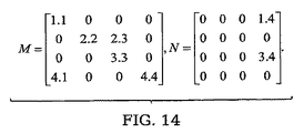
行列Jexampleは、最後に順序付けられた頂点セパレータに対応する列をスプリットアウトする(分け出す)ことでスプリットすることができる。このような列をスプリットするためには、当該列の非対角エントリだけをスプリットアウトすればよい。スプリットアウトされた行列をNと表記し、残りのメインの行列をMと表記する。我々の例では、図14に示すようにJexample=M+Nとなる。 The matrix J example can be split by splitting out (separating) the column corresponding to the last ordered vertex separator. In order to split such a column, only the non-diagonal entries of that column need be split out. The split-out matrix is denoted as N, and the remaining main matrix is denoted as M. In our example, J example = M + N as shown in FIG.
MがM=LUのようなLU分解をもつとする。下行列Lは、次のように回路シミュレーションにおいて線形系をプレコンディションするために使うことができる。 Let M have an LU decomposition such that M = LU. The lower matrix L can be used to precondition a linear system in circuit simulation as follows.
![]()
![]()
図15は、線形化されプレコンディションされた回路方程式(U+L−1N)x=L−1rを解くためのフローチャート250を示す。手続きは開始ブロック252で示されるように始まり、オペレーション254に進み、L−1Nが次のように二つの部分にスプリットされる。
FIG. 15 shows a
![]()
![]()
第1の部分EはL−1Nの計算の後、相対的に大きな値になるエントリからなる。第2の部分L−1Fは相対的に小さいエントリからなる。このスプリッティングは、L−1Nの計算過程でエントリの値を比較することで形成される。回路シミュレーションにおいて解くべき線形系は次のようになる。 The first part E consists of entries that have a relatively large value after the calculation of L −1 N. The second part L −1 F consists of relatively small entries. This splitting is formed by comparing the values of entries in the process of calculating L −1 N. The linear system to be solved in the circuit simulation is as follows.
![]()
![]()
次に、オペレーション256において、線形系は(U+E)でプレコンディションされ、次のプレコンディションされた系を形成するようになる。
Next, in
![]()
![]()
EとFは頂点セパレータに対応する最後の列においてだけ非ゼロの値をもつことに留意すべきである。したがって、行列U+Eは、頂点セパレータに対応する最後のブロックを除いて上三角形式である。この線形系において、頂点セパレータに対応する部分系は独立である。 Note that E and F have non-zero values only in the last column corresponding to the vertex separator. Therefore, the matrix U + E is an upper triangular expression except for the last block corresponding to the vertex separator. In this linear system, the subsystem corresponding to the vertex separator is independent.
最後に、オペレーション258において、GMRESのようなKrylov部分空間反復法を適用して部分系を解く。各反復において、次の行列−ベクトル積が計算される。
Finally, in
![]()
![]()
ここで、|subsystemは、ベクトルの部分系への射影を示す。F・xを計算する際、x|subsystemだけが寄与する。なぜなら、Fの非ゼロの列だけが部分系に対応するものであるからである。このことはまた、部分系が独立である理由を説明している。行列Lの逆行列を求める際、分離されたパーティションに対応する対角ブロックの逆行列を並列に求めることができる。行列−ベクトル積である(U+E)−1・(L−1Fx)を計算する際、次の系が解かれる。 Here, | subsystem indicates the projection of a vector onto a subsystem . In calculating F · x, only x | subsystem contributes. This is because only non-zero columns of F correspond to subsystems. This also explains why the subsystems are independent. When obtaining an inverse matrix of the matrix L, inverse matrices of diagonal blocks corresponding to the separated partitions can be obtained in parallel. When calculating (U + E) −1 · (L −1 Fx), which is a matrix-vector product, the following system is solved.
![]()
![]()
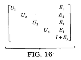
ここで、L−1Fxは既に計算されたベクトルである。Uの対角は1を含み、頂点セパレータに対応するUの最後のブロックは1の対角成分だけをもつ。たとえば、行列が4つのパーティションをもつとする。この場合、U+Eは図16に示す構造をもつ。この系を解くために、頂点セパレータに対応する最後のブロックI+E5が最初に解かれる。この部分系は独立であることに留意する。 Here, L −1 Fx is a vector that has already been calculated. The diagonal of U contains 1 and the last block of U corresponding to the vertex separator has only 1 diagonal component. For example, assume that a matrix has four partitions. In this case, U + E has the structure shown in FIG. To solve this system, the last block I + E 5 corresponding to the vertex separator is solved first. Note that this subsystem is independent.
我々のKrylov部分空間ベクトルの長さは、縮小された部分系のサイズのことであるが、Saadの方法ではKrylov部分空間ベクトルの長さは、「背景」の節で説明したように、元の行列のサイズのことである。 The length of our Krylov subspace vector is the size of the reduced subsystem, but in the Saad method, the length of the Krylov subspace vector is the original, as explained in the “Background” section. It is the size of the matrix.
縮小された部分系を解くために直接解法を用いることは都合がよいことを留意すべきである。それは、縮小された系が非常に疎であるときに意味がある。こうすることにより、その方法は純粋な直接法になる。非常に疎な行列に対して、直接解法は反復解法よりも高速になりうる。ここで述べる方法がこの柔軟性をもつことは有利であり、そのことは直接・反復ハイブリッド法のユニークな特徴である。 It should be noted that it is convenient to use a direct solution to solve the reduced subsystem. It makes sense when the reduced system is very sparse. This makes the method a pure direct method. For very sparse matrices, the direct solution can be faster than the iterative solution. It is advantageous that the method described here has this flexibility, which is a unique feature of the direct and iterative hybrid method.
部分系xsubsystemに対する解が得られた後、後ろ向き代入を用いて、その系を縮小することができる。残りの系を解く際、個別のパーティションに対応するブロックは並列に解かれる。系に対する解は次のように得られる。 After the solution for the subsystem xsubsystem is obtained, the system can be reduced using backward substitution. When solving the rest of the system, the blocks corresponding to the individual partitions are solved in parallel. The solution for the system is obtained as follows.
図15を参照して上述した、直接・反復ハイブリッド法を含む行列解法技術は、部分行列I+E5の逆行列を求めるまたはこれを解くときに適用することができる。もし部分行列I+E5のサイズがまだ大きすぎるなら、部分行列が疎であることを保ち、その計算に並列性をさらに求められるように、この方法を再帰的に適用することができる。各再帰ステップにおいて、縮小された部分系のサイズはさらに小さくなる。縮小された部分系のサイズが予め定めた閾値よりも小さくなったとき、あるいは、部分系が行列特性解析を通じて直接解法にとって効率的であると判定されたとき、再帰は停止する。この時点で直接法は、最終的な小さな部分系に適用され、この手続きは完了ブロック260で示されるように終了する。たとえば、ある実施の形態では、直説法は、部分系の行列が100行以下になったときに適用される。別の実施の形態では、直説法は、部分系の行列のLU分解が生成するフィル−インの数が小さくなったときに適用される。
Described above with reference to FIG. 15, matrix solution techniques including hybrid direct and iterative methods can be applied when solving obtaining or containing the inverse matrix of the partial matrix I + E 5. If the size of the partial matrix I + E 5 is still too high, keeping the partial matrix is sparse, so further determined parallelism in the calculation, this method can be applied recursively. At each recursion step, the size of the reduced subsystem is further reduced. The recursion stops when the size of the reduced subsystem becomes smaller than a predetermined threshold or when the subsystem is determined to be efficient for direct solution through matrix property analysis. At this point, the direct method is applied to the final small subsystem and the procedure ends as indicated by
シミュレーション行列が巨大であり、依然として疎に群がっていることがありうるから、Krylov部分空間法が部分系レベルで適用される。ここで述べる方法において、列が結合(カップリング)に対応している行列ブロックNに、スプリッティング技術が適用され、行列ブロックNは元の線形系レベルになる。それに加えて、上述の方法がE(L−1Nの一部)の計算において列ベースになる。結果として、この実装は、共有メモリ型並列コンピュータ上で並列化するのが簡単である。 The Krylov subspace method is applied at the subsystem level because the simulation matrix is huge and may still be sparsely clustered. In the method described here, a splitting technique is applied to the matrix block N whose columns correspond to coupling (coupling), and the matrix block N becomes the original linear system level. In addition, the method described above is column-based in the calculation of E (part of L −1 N). As a result, this implementation is easy to parallelize on a shared memory parallel computer.
この方法の一つの利点は、Krylov部分空間法をサイズが巨大であるトップレベルの回路行列Jには適用しないことである。その代わりにKrylov部分空間法をサイズがずっと小さい結合部分系に適用する。しかし、可能な限り元の回路行列を疎に保つためにスプリッティングがL−1Nの計算に適用される。これは、トップレベルの回路線形系のサイズをもつKrylov部分空間ベクトルを記憶し、直交化する問題を解く。したがって、今述べているアプローチは巨大な回路行列を解くための直接法および反復法の両方の利点を活用することができる。 One advantage of this method is that the Krylov subspace method is not applied to the top-level circuit matrix J, which is huge in size. Instead, the Krylov subspace method is applied to coupled subsystems that are much smaller in size. However, splitting is applied to the calculation of L −1 N in order to keep the original circuit matrix as sparse as possible. This solves the problem of storing and orthogonalizing the Krylov subspace vector with the size of the top level circuit linear system. Thus, the approach just described can take advantage of both direct and iterative methods for solving large circuit matrices.
この数値的方法は、以下で述べる柔軟なデータ構造と相まって、行列解法が回路シミュレーションにおいて効率的な過渡シミュレーションを提供することを保証する。過渡シミュレーションでは、異なる非ゼロの値をもつ行列を何度も解く必要がある。本アプローチは行列スプリッティングを動的に扱う点で柔軟性を有する。以下述べるように、本アプローチはまた、静的、周期的、準周期的シミュレーションにとって好適である。 This numerical method, coupled with the flexible data structure described below, ensures that the matrix solution provides an efficient transient simulation in circuit simulation. In transient simulation, it is necessary to solve a matrix with different non-zero values many times. This approach is flexible in that it handles matrix splitting dynamically. As described below, this approach is also suitable for static, periodic, and quasi-periodic simulations.
[スプリッティングのための動的なデータ構造] [Dynamic data structure for splitting]
行列E、F1およびF2は非常に動的である。具体的には、シミュレーション過程のあらゆるステップで変わるかもしれない。効率的で柔軟なデータストレージを実現するために、ハッシュテーブルを用いてもよい。行列の列ベクトルの各エントリに対して、元の列ベクトルにおける行インデックス、コンパクトベクトル(非ゼロ)におけるインデックス、およびその値を格納してもよい。ある実施の形態では、たとえば、行列の各列を格納するためにC++のSTLライブラリのMapまたはVectorを用いる。 The matrices E, F 1 and F 2 are very dynamic. Specifically, it may change at every step of the simulation process. In order to realize efficient and flexible data storage, a hash table may be used. For each entry in the matrix column vector, the row index in the original column vector, the index in the compact vector (non-zero), and its value may be stored. In one embodiment, for example, a C ++ STL library Map or Vector is used to store each column of the matrix.
ハッシュテーブルはまた、全体系において部分系に属するインデックスを格納するために用いてもよい。Vectorは結合インデックス集合ICを格納するために使ってもよい。ハッシュテーブルを用いることの一つの利点は、全体系のサイズがどれだけ巨大であったとしても、格納する必要のあるインデックスの数は制限されることである。さらに、インデックスがこの集合に属するかどうかは線形時間で決定することができる。 The hash table may also be used to store an index belonging to a partial system in the entire system. Vector can be used to store the binding index set I C. One advantage of using a hash table is that no matter how large the overall system size is, the number of indexes that need to be stored is limited. Furthermore, whether an index belongs to this set can be determined in linear time.
別の実施の形態において、バイナリツリーを動的なデータ構造のために用いる。バイナリサーチツリーを用いることにより、インデックスは常に順序づけが保たれ、ツリーをある順序で容易に行き来することができるようになる。このデータ構造を用いることにより、ツリーに挿入することがlog(n)の時間で行える。ここでnはツリーのサイズである。nがそれほど大きくないなら、このCPU時間は受け入れ可能である。同様に、ツリーにおけるエントリやインデックスの場所もlog(n)の時間で見つけることができる。 In another embodiment, a binary tree is used for dynamic data structures. By using a binary search tree, the index is always ordered and the tree can be easily traversed in a certain order. By using this data structure, insertion into the tree can be performed in log (n) time. Here, n is the size of the tree. This CPU time is acceptable if n is not too large. Similarly, the location of entries and indexes in the tree can be found in log (n) time.
こういった動的なデータ構造は、行列E、F1およびF2を構築するのに役立つ。我々はこれらの行列の構築の効率性を保つことができる。 These dynamic data structures help to build the matrices E, F 1 and F 2 . We can keep the efficiency of building these matrices.
[並列マルチレートシミュレーション] [Parallel multirate simulation]
集積回路はその機能においてマルチレートの振る舞いをする。マルチレートの振る舞いをするのは、集積回路がオペレーションの過程で高周波と低周波の両方を取り扱うという事実による。 Integrated circuits behave multi-rate in function. The multi-rate behavior is due to the fact that integrated circuits handle both high and low frequencies during operation.
回路シミュレーションにおいて、高周波信号は解くにはより多くのタイムステップが必要であるが、低周波信号はより少ないタイムステップで解くことができる。さらに、デジタルライクな信号に対しては、エッジは解くためにより多くのタイムステップが必要であるが、フラットな領域は解くのにほとんどタイムステップを必要としない。従来のSpiceタイプの回路シミュレーションでは、その特性は利用することができない。なぜなら全体回路は分割されていないし、回路方程式を離散化するにあたり、グローバルタイムステップが適用されるからである。正確さを保証するためには、最小タイムステップをシミュレーションで適用しなければならない。シミュレーションがより多くのタイムステップを取れば取るほど、速度が遅くなる。 In circuit simulation, a high frequency signal requires more time steps to solve, while a low frequency signal can be solved with fewer time steps. Furthermore, for digital-like signals, more time steps are required to solve the edges, but flat regions require little time steps to solve. The characteristic cannot be used in the conventional Spice type circuit simulation. This is because the entire circuit is not divided and a global time step is applied to discretize the circuit equation. In order to ensure accuracy, a minimum time step must be applied in the simulation. The more time steps the simulation takes, the slower it gets.
従来のSpiceタイプの回路シミュレーションを高速化するために、FastMos回路シミュレータは全体の回路を異なるパーティションに分割し、マルチレートの振る舞いを利用するために異なるパーティションに異なるタイムステップを割り当てる。あるパーティションにおける信号が高周波であるなら、シミュレーションにおいて小さなタイムステップを取る。別のパーティションにおける信号が低周波であるなら、シミュレーションにおいて大きなタイムステップを取る。このマルチレートシミュレーション法を実装する際、FastMOSシミュレータはイベント駆動型のスキームを採用する。イベント駆動型スキームはイベント伝搬にしたがって、解くべきパーティションすなわち部分回路を決定する。もしあるパーティションでイベントが起こるなら、そのパーティションは一つの反復または一つのタイムステップの間、シミュレートされる。 In order to speed up the conventional Spice type circuit simulation, the FastMos circuit simulator divides the entire circuit into different partitions and assigns different time steps to different partitions to take advantage of multi-rate behavior. If the signal in a partition is high frequency, take a small time step in the simulation. If the signal in another partition is low frequency, take a large time step in the simulation. When implementing this multi-rate simulation method, the FastMOS simulator employs an event-driven scheme. Event driven schemes determine partitions or subcircuits to be solved according to event propagation. If an event occurs in a partition, that partition is simulated for one iteration or one time step.
イベント駆動型スキームはシミュレートすべきパーティションをシミュレートするだけである。そのため、不必要な計算を省くことができ、従来のSpiceシミュレータに比べてかなりスピードアップを図ることできる。しかし、深刻な欠点はイベントフローがシリアルである、すなわち、あるイベントの発生が以前のイベントに依存することである。この分野における公知の試みは、波形緩和および楽観的スケジューリングである。これらの技術は一般的な回路シミュレーションに対して積極的過ぎて成功しない。 The event driven scheme only simulates the partition to be simulated. Therefore, unnecessary calculations can be omitted, and the speed can be considerably increased as compared with the conventional Speed simulator. However, a serious drawback is that the event flow is serial, that is, the occurrence of an event depends on previous events. Known attempts in this field are waveform relaxation and optimistic scheduling. These techniques are too aggressive for general circuit simulation and are not successful.
あるイベントのシミュレーションを並列化することは、関わる計算量がほんのわずかであるため、解決策とはならない。あるイベントをシミュレーションするための仕事量は基本的には、あるタイムステップの間、あるパーティションをシミュレーションする際に関わる仕事量である。一般的に、これらのパーティションはFastMOSシミュレーションではたいへん小さい。たとえば、一つのパーティションで二つのトランジスタがあるだけである。このような小さな量のシミュレーションの仕事を並列化しても、期待に沿うような並列効率性を達成することはできない。 Parallelizing the simulation of an event is not a solution because it involves only a small amount of computation. The amount of work for simulating an event is basically the amount of work involved in simulating a partition during a time step. In general, these partitions are very small in the FastMOS simulation. For example, there are only two transistors in one partition. Even if such a small amount of simulation work is parallelized, parallel efficiency as expected can not be achieved.
ここで例示の目的で説明した並列マルチレートシミュレーションスキームにおいて、イベント駆動型スキームは使われていない。その代わり、すべてのアクティブなパーティションが一緒に解かれる。このアクティブなパーティションのグループは、各タイムステップにおいて各非線形反復過程で動的に成長することがある。 In the parallel multi-rate simulation scheme described here for exemplary purposes, an event driven scheme is not used. Instead, all active partitions are solved together. This group of active partitions may grow dynamically with each non-linear iterative process at each time step.
周期的に訂正ステップが実行される。この訂正ステップにおいて、複数のタイムステップが正確さを向上させて一緒に解かれる。上述の並列行列ソルバー(solver)を、多くのパーティションと数多くのステップを必要とする結合系を切り離す(decouple)ために使ってもよい。もし強引(brute-force)な直接法または反復法で系を解くなら、計算は非常に遅くなるか非効率的になる。シューティング−ニュートン(shooting-Newton)RFシミュレーションアルゴリズムにおいて使われるものに似た反復法は、あまりに非効率であろう。そのような強引な反復法において、対角および部分対角ブロックをプレコンディショナーとしてもつ線形系を解くためにKrylov部分空間法を用いるであろう。この場合、結合(カップリング)はプレコンディショニング解法において考慮されない。このように強引な方法は大きな回路をシミュレートするには遅く、不適当である。 Periodically correction steps are performed. In this correction step, multiple time steps are solved together with improved accuracy. The parallel matrix solver described above may be used to decouple coupled systems that require many partitions and many steps. If the system is solved by a brute-force direct or iterative method, the computation will be very slow or inefficient. An iterative method similar to that used in the Shooting-Newton RF simulation algorithm would be too inefficient. In such an aggressive iterative method, the Krylov subspace method will be used to solve linear systems with diagonal and partial diagonal blocks as preconditioners. In this case, coupling is not considered in the preconditioning solution. This aggressive method is slow and unsuitable for simulating large circuits.
[いろいろなタイプの回路シミュレーションにおけるアプリケーション] [Applications for various types of circuit simulation]
過渡的な回路シミュレーションに加えて、並列行列ソルバーを静的な回路シミュレーション(DC回路シミュレーション、周期的あるいは準周期的な定常状態RFシミュレーションと呼ばれることもある)に適用することができる。DCシミュレーションのある実施の形態(疑似過渡DCシミュレーションと呼ばれる)において、電圧源と電流源を0値からDC値まで上昇させる。それから、シミュレーションは、DC解である定常状態に到達するまで続けられる。DCシミュレーションの別の実施の形態では、我々の方法を次の静的な回路方程式を解くために適用することができる。 In addition to transient circuit simulation, the parallel matrix solver can be applied to static circuit simulation (also called DC circuit simulation, periodic or quasi-periodic steady state RF simulation). In one embodiment of DC simulation (referred to as quasi-transient DC simulation), the voltage and current sources are raised from a zero value to a DC value. The simulation is then continued until a steady state is reached, which is a DC solution. In another embodiment of DC simulation, our method can be applied to solve the following static circuit equation:
これは動的な部分がない方程式1である。
This is
並列行列ソルバーはRF(radio frequency)回路シミュレーションに適用することもできる。有限差分法やシューティング−ニュートン法のようなRF回路シミュレーション方法は、いくつかのタイムインターバルにおいて周期的または準周期的解を求めるために解く。その目的のため、周期的または準周期的境界条件がない方程式1を解く。周期的定常状態を例に取ると、境界条件はv(t1)=v(t2)である。ここで[t1,t2]は周期的なタイムインターバルである。有限差分法またはシューティング−ニュートン法はこの境界条件を満たす解を求める。ここで、上述の行列ソルバーを線形化された線形系を解くために使ってもよい。
The parallel matrix solver can also be applied to RF (radio frequency) circuit simulation. RF circuit simulation methods such as the finite difference method and the Shooting-Newton method are solved to obtain periodic or quasi-periodic solutions in several time intervals. To that end, we solve
[コンピュータ実装] [Computer implementation]
上記の実施の形態を念頭において、本発明は、コンピュータシステムに記憶されたデータに関係するコンピュータ実装された様々なオペレーションを利用することができることが理解されよう。これらのオペレーションは物理的な量の物理的操作を要求するものである。通常、必ずしもそうとは限らないが、こういった量は、保存、転送、結合、比較、さもなければ操作が可能な電気的もしくは磁気的な信号の形を取る。さらに、実行される操作は生産、特定、決定、比較のような用語で参照されることがある。 With the above embodiments in mind, it will be appreciated that the present invention can utilize a variety of computer-implemented operations relating to data stored in a computer system. These operations are those requiring physical manipulation of physical quantities. Usually, though not necessarily, these quantities take the form of electrical or magnetic signals capable of being stored, transferred, combined, compared, and otherwise manipulated. Furthermore, the operations performed may be referred to in terms such as production, identification, determination, comparison.
ここで記述した本発明の一部を形成するオペレーションはいずれも有用なマシーンオペレーションである。本発明はまた、これらのオペレーションを実行するためのデバイスまたは装置に関する。装置は要求された目的のために特別に構成することができる。あるいは、装置は、コンピュータに記憶されたコンピュータプログラムによって選択的に活性化したり、構成したりすることができる汎用のコンピュータであってもよい。特に、ここで述べた教示内容に沿って書かれたコンピュータプログラムをもつ様々な汎用マシーンを用いることができる。あるいは、要求されたオペレーションを実行するためにより特化した装置を構成するとより便利である。 Any of the operations that form part of the invention described herein are useful machine operations. The present invention also relates to a device or apparatus for performing these operations. The device can be specially configured for the required purpose. Alternatively, the apparatus may be a general-purpose computer that can be selectively activated or configured by a computer program stored in the computer. In particular, various general purpose machines having computer programs written in accordance with the teachings described herein can be used. Alternatively, it is more convenient to configure a more specialized device to perform the requested operation.
本発明はコンピュータ読み取り可能な媒体上のコンピュータ読み取り可能なコードとして具体化することができる。コンピュータ読み取り可能な媒体は、データを記憶する任意のデータストレージデバイスであり、コンピュータシステムによって読み取ることができる。コンピュータ読み取り可能な媒体はまた、コンピュータコードが具体化された電磁搬送波を含む。コンピュータ読み取り可能な媒体の例として、ハードドライブ、ネットワーク接続ストレージ(NAS)、リードオンリーメモリ、ランダムアクセスメモリ、CD−ROM、CD−R、CD−RW、磁気テープ、その他のオプティカル/非オプティカルデータストレージデバイスがある。コンピュータ読み取り可能な媒体をネットワーク接続されたコンピュータシステム上に分散させ、コンピュータ読み取り可能なコードを分散方式で保存し、実行するようにもできる。 The present invention can be embodied as computer readable code on a computer readable medium. The computer readable medium is any data storage device that stores data, which can be read by a computer system. The computer readable medium also includes an electromagnetic carrier wave having computer code embodied therein. Examples of computer readable media include hard drives, network attached storage (NAS), read only memory, random access memory, CD-ROM, CD-R, CD-RW, magnetic tape, and other optical / non-optical data storage There is a device. Computer readable media may be distributed over networked computer systems so that computer readable code is stored and executed in a distributed fashion.
本発明の実施の形態は、単一のコンピュータで処理することができ、また、複数のコンピュータまたは相互接続されたコンピュータコンポーネントを用いて処理することができる。ここで使われるコンピュータとは、プロセッサ、メモリ、ストレージをもつスタンドアロンのコンピュータ、または、ネットワーク端末にコンピュータリソースを提供する分散コンピューティングシステムを含む。ある分散コンピューティングシステムでは、コンピュータシステムのユーザは、現実には多くのユーザ間で共有されているコンポーネント部分にアクセスしている。したがって、ユーザはネットワーク上で仮想コンピュータにアクセスすることができ、ユーザには、一人のユーザに対してカスタマイズされた専用の単一のコンピュータとして見える。 Embodiments of the present invention can be processed on a single computer and can be processed using multiple computers or interconnected computer components. As used herein, a computer includes a stand-alone computer having a processor, memory, and storage, or a distributed computing system that provides computer resources to a network terminal. In some distributed computing systems, computer system users have access to component parts that are actually shared among many users. Thus, the user can access the virtual computer over the network and appears to the user as a dedicated single computer customized for a single user.
前述の発明は、明確に理解するために詳細に記述したが、添付の請求項の範囲内で変更や修正をすることができることは明らかである。したがって、本実施の形態は例示と考えるべきであり、限定的に捉えるべきものではない。本発明はここで説明した詳細な内容に限定されるものではなく、添付の請求項の範囲およびその均等の範囲で変更することができる。 Although the foregoing invention has been described in detail for purposes of clarity of understanding, it will be apparent that changes and modifications may be practiced within the scope of the appended claims. Therefore, this embodiment should be considered as an example, and should not be taken as limited. The present invention is not limited to the detailed contents described herein but can be modified within the scope of the appended claims and their equivalents.
Claims (47)
集積回路のオペレーションをモデル化する微分代数方程式(DAE)の系を生成するステップと、
前記DAEの系を離散化するステップと、
前記DAEが非線形である場合、離散化されたDAEを線形化して回路ヤコビ行列をもつ線形系を形成するステップと、
線形化された回路ヤコビ行列ソルバーを用いて前記線形系を解くステップとを含み、
前記線形系を解くステップは、
前記回路ヤコビ行列を二つの行列MとNにスプリットするステップと、
対角成分が1で非対角成分がゼロの恒等行列をIとして、前記二つの行列をプレコンディションしてI+M−1Nの形の行列をもつプレコンディションされた方程式を形成するステップと、
直接・反復組み合わせ解法を用いて前記プレコンディションされた方程式におけるI+M−1Nに対する解を求めるステップとを含むことを特徴とする方法。 A computer-implemented method for integrated circuit simulation operation comprising:
Generating a system of differential algebraic equations (DAE) that models the operation of the integrated circuit;
Discretizing the DAE system;
If the DAE is non-linear, linearizing the discretized DAE to form a linear system with a circuit Jacobian matrix;
Solving the linear system using a linearized circuit Jacobian solver,
Solving the linear system comprises:
Splitting the circuit Jacobian matrix into two matrices M and N;
Preconditioning the two matrices to form a preconditioned equation having a matrix of the form I + M −1 N, where I is an identity matrix with diagonal component 1 and non-diagonal component zero;
Determining a solution for I + M −1 N in the preconditioned equation using a direct and iterative combined solution.
前記解を前記離散化された方程式に代入して複数のノードのそれぞれに対して電圧の変化を求めるステップと、
前記DAEの有限差分離散化と非線形反復法を用いて電圧の変化を解くための前記線形系を求めるステップと、
複数のノードのそれぞれに対して電圧の変化を現在の電圧ベクトルに足すことにより、各ノードの新しい電圧値を与える新しい電圧ベクトルを求めるステップと、
次のタイムステップでDAEの新しい系を解くために1タイムステップ進め、続くタイムステップに対して当該解くステップを繰り返すことにより、集積回路の過渡的な振る舞いをモデル化するステップとを含むことを特徴とする請求項2の方法。 The step of solving the DAE system further includes:
Substituting the solution into the discretized equation to determine a change in voltage for each of a plurality of nodes;
Determining the linear system for solving voltage changes using the DAE finite difference discretization and a non-linear iterative method;
Determining a new voltage vector that gives a new voltage value for each node by adding the change in voltage to the current voltage vector for each of the plurality of nodes;
Including the step of modeling the transient behavior of an integrated circuit by advancing one time step to solve a new system of DAEs at the next time step and repeating the solving step for subsequent time steps. The method of claim 2.
Uを上三角行列、Lを下三角行列として、M−1をU−1L−1に置き換えることにより項U−1L−1Nを形成するステップと、
U−1L−1Nを第1、第2、第3の三つの部分にスプリットするステップとを含み、
前記第1の部分は行列の相対的に大きい値であるエントリを含み、前記第2の部分と前記第3の部分は、計算過程で相対的に小さな値であるエントリを含むことを特徴とする請求項1の方法。 The step of solving the matrix I + M −1 N is
Forming the term U −1 L −1 N by replacing M −1 with U −1 L −1 with U as the upper triangular matrix and L as the lower triangular matrix;
Splitting U −1 L −1 N into first, second and third parts,
The first part includes an entry having a relatively large value in the matrix, and the second part and the third part include entries having a relatively small value in a calculation process. The method of claim 1.
F2は、U−1L−1N=U−1(E0+L−1F1)=E+U−1F2+U−1L−1F1の計算過程で形成されることを特徴とする請求項6の方法。 F 1 is formed in the calculation process of L −1 N = E 0 + L −1 F 1 ,
F 2 is formed in the calculation process of U −1 L −1 N = U −1 (E 0 + L −1 F 1 ) = E + U −1 F 2 + U −1 L −1 F 1. The method of claim 6.
縮小された部分系のサイズが所定の閾値より小さくなるか、縮小された部分系が行列特性解析を通じて直接解法にとって効率的であると判定されたとき、再帰を停止するステップとをさらに含むことを特徴とする請求項19の方法。 Reordering the circuit Jacobian matrix, splitting the circuit Jacobian matrix into matrices M and N to form a preconditioned circuit equation, and using the lower matrix L to form a preconditioned circuit equation And recursively executing a series of operations including solving a preconditioned circuit equation by splitting L −1 N into two parts and preconditioning the system with a preconditioner (U + E); ,
Further comprising the step of stopping recursion when the size of the reduced subsystem is less than a predetermined threshold, or when the reduced subsystem is determined to be efficient for direct solution through matrix characterization. 20. A method according to claim 19 characterized in that:
複数のノードのそれぞれにおける電圧の値を含む電圧ベクトルと前記回路ヤコビ行列を前記パーティションにしたがってリオーダーするためのインストラクションと、
前記回路ヤコビ行列を二つの行列MとNにスプリットするためのインストラクションと、
対角成分が1で非対角成分がゼロの恒等行列をIとして、前記二つの行列をプレコンディションしてI+M−1Nの形の行列をもつプレコンディションされた方程式を形成するためのインストラクションと、
直接・反復組み合わせ解法を用いて前記プレコンディションされた方程式におけるI+M−1Nに対する解を求めるためのインストラクションとを含むことを特徴とするマシーン読み取り可能媒体。 Machine-readable recorded program instructions that cause a computer system to solve a system of differential algebraic equations (DAEs) that model the operation of an integrated circuit using a circuit Jacobian matrix divided into loosely coupled partitions The medium, the machine-readable medium is
A voltage vector including a voltage value at each of a plurality of nodes and instructions for reordering the circuit Jacobian matrix according to the partition;
Instructions for splitting the circuit Jacobian matrix into two matrices M and N;
Instructions for preconditioning the two matrices to form a preconditioned equation having a matrix of the form I + M −1 N, where I is an identity matrix with a diagonal component of 1 and a non-diagonal component of zero. When,
Machine readable medium comprising a instructions for finding a solution to I + M -1 N in the preconditioned equation using the direct and iterative combinations solution.
Uを上三角行列、Lを下三角行列として、M−1をU−1L−1に置き換えることにより項U−1L−1Nを形成するためのインストラクションと、
U−1L−1Nを第1、第2、第3の三つの部分にスプリットするためのインストラクションとを含み、
前記第1の部分は行列の相対的に大きい値であるエントリを含み、前記第2の部分と前記第3の部分は、計算過程で相対的に小さな値であるエントリを含むことを特徴とする請求項26のマシーン読み取り可能媒体。 Instructions for solving the matrix I + M −1 N are
Instructions for forming the term U −1 L −1 N by replacing M −1 with U −1 L −1 with U as the upper triangular matrix and L as the lower triangular matrix;
Instructions for splitting U −1 L −1 N into first, second and third parts,
The first part includes an entry having a relatively large value in the matrix, and the second part and the third part include entries having a relatively small value in a calculation process. 27. The machine readable medium of claim 26.
F2は、U−1L−1N=U−1(E0+L−1F1)=E+U−1F2+U−1L−1F1の計算過程で形成されることを特徴とする請求項29のマシーン読み取り可能媒体。 F 1 is formed in the calculation process of L −1 N = E 0 + L −1 F 1 ,
F 2 is formed in the calculation process of U −1 L −1 N = U −1 (E 0 + L −1 F 1 ) = E + U −1 F 2 + U −1 L −1 F 1. 30. The machine readable medium of claim 29.
再帰の停止の後、直接法によって前記縮小された部分系を解くためのインストラクションとをさらに含むことを特徴とする請求項33のマシーン読み取り可能媒体。 Instructions to determine whether to stop recursion based on the size of the reduced subsystem, or whether the reduced subsystem is efficient for direct solution through matrix characterization, and
34. The machine readable medium of claim 33, further comprising instructions for solving the reduced subsystem by a direct method after stopping recursion.
Δvは回路ノードにおける以前の近似からの電圧の変化を含むベクトルを表し、
Δv represents a vector containing the change in voltage from the previous approximation at the circuit node,
縮小された部分系のサイズ、あるいはその縮小された部分系が行列特性解析を通じて直接解法にとって効率的であるかどうかの判定にもとづいて、再帰を停止するかどうかを決定するためのインストラクションと、
再帰の停止の後、直接法によって前記縮小された部分系を解くためのインストラクションとをさらに含むことを特徴とする請求項41のマシーン読み取り可能媒体。 Instructions for reordering the circuit Jacobian matrix, instructions for splitting the circuit Jacobian matrix into matrices M and N to form a preconditioned circuit equation, and a lower matrix L to form a preconditioned circuit equation Recursively execute instructions to solve preconditioned circuit equations by splitting L -1 N into two parts and preconditioning the system with a preconditioner (U + E) Instruction steps to do
Instructions to determine whether to stop recursion based on the size of the reduced subsystem, or whether the reduced subsystem is efficient for direct solution through matrix characterization, and
42. The machine-readable medium of claim 41, further comprising instructions for solving the reduced subsystem by a direct method after stopping recursion.
Applications Claiming Priority (5)
| Application Number | Priority Date | Filing Date | Title |
|---|---|---|---|
| US75221705P | 2005-12-19 | 2005-12-19 | |
| US60/752,217 | 2005-12-19 | ||
| US78937606P | 2006-04-04 | 2006-04-04 | |
| US60/789,376 | 2006-04-04 | ||
| PCT/US2006/048551 WO2007075757A2 (en) | 2005-12-19 | 2006-12-18 | Parallel multi-rate circuit simulation |
Publications (2)
| Publication Number | Publication Date |
|---|---|
| JP2009520306A true JP2009520306A (en) | 2009-05-21 |
| JP4790816B2 JP4790816B2 (en) | 2011-10-12 |
Family
ID=38218555
Family Applications (1)
| Application Number | Title | Priority Date | Filing Date |
|---|---|---|---|
| JP2008547473A Active JP4790816B2 (en) | 2005-12-19 | 2006-12-18 | Parallel multirate circuit simulation |
Country Status (5)
| Country | Link |
|---|---|
| US (1) | US7783465B2 (en) |
| EP (1) | EP1964010B1 (en) |
| JP (1) | JP4790816B2 (en) |
| TW (1) | TWI340906B (en) |
| WO (1) | WO2007075757A2 (en) |
Families Citing this family (20)
| Publication number | Priority date | Publication date | Assignee | Title |
|---|---|---|---|---|
| US8711146B1 (en) * | 2006-11-29 | 2014-04-29 | Carnegie Mellon University | Method and apparatuses for solving weighted planar graphs |
| US20080208553A1 (en) * | 2007-02-27 | 2008-08-28 | Fastrack Design, Inc. | Parallel circuit simulation techniques |
| US8091052B2 (en) * | 2007-10-31 | 2012-01-03 | Synopsys, Inc. | Optimization of post-layout arrays of cells for accelerated transistor level simulation |
| US8543360B2 (en) | 2009-06-30 | 2013-09-24 | Omniz Design Automation Corporation | Parallel simulation of general electrical and mixed-domain circuits |
| TWI476616B (en) * | 2010-02-12 | 2015-03-11 | Synopsys Shanghai Co Ltd | Estimation Method and Device of Initial Value for Simulation of DC Working Point |
| CN101937481B (en) * | 2010-08-27 | 2012-02-01 | 天津大学 | Transient simulation method of distributed power generation system based on automatic differentiation technology |
| US8555229B2 (en) | 2011-06-02 | 2013-10-08 | International Business Machines Corporation | Parallel solving of layout optimization |
| US20130226535A1 (en) * | 2012-02-24 | 2013-08-29 | Jeh-Fu Tuan | Concurrent simulation system using graphic processing units (gpu) and method thereof |
| US9117043B1 (en) * | 2012-06-14 | 2015-08-25 | Xilinx, Inc. | Net sensitivity ranges for detection of simulation events |
| US9135383B2 (en) * | 2012-11-16 | 2015-09-15 | Freescale Semiconductor, Inc. | Table model circuit simulation acceleration using model caching |
| US9170836B2 (en) | 2013-01-09 | 2015-10-27 | Nvidia Corporation | System and method for re-factorizing a square matrix into lower and upper triangular matrices on a parallel processor |
| US20150178438A1 (en) * | 2013-12-20 | 2015-06-25 | Ertugrul Demircan | Semiconductor manufacturing using design verification with markers |
| CN105205191B (en) * | 2014-06-12 | 2018-10-12 | 济南概伦电子科技有限公司 | Multi tate parallel circuit emulates |
| JP6384331B2 (en) * | 2015-01-08 | 2018-09-05 | 富士通株式会社 | Information processing apparatus, information processing method, and information processing program |
| JP6803173B2 (en) * | 2015-08-24 | 2020-12-23 | エスエーエス アイピー,インコーポレーテッドSAS IP, Inc. | Processor execution system and method for time domain decomposition transient simulation |
| US10867008B2 (en) * | 2017-09-08 | 2020-12-15 | Nvidia Corporation | Hierarchical Jacobi methods and systems implementing a dense symmetric eigenvalue solver |
| US11663383B2 (en) * | 2018-06-01 | 2023-05-30 | Icee Solutions Llc. | Method and system for hierarchical circuit simulation using parallel processing |
| EP3803644A4 (en) * | 2018-06-01 | 2022-03-16 | ICEE Solutions LLC | Method and system for hierarchical circuit simulation using parallel processing |
| CN112949232A (en) * | 2021-03-17 | 2021-06-11 | 梁文毅 | Electrical simulation method based on distributed modeling |
| CN117077607A (en) * | 2023-07-26 | 2023-11-17 | 南方科技大学 | Large-scale linear circuit simulation method, system, circuit simulator and storage medium |
Citations (1)
| Publication number | Priority date | Publication date | Assignee | Title |
|---|---|---|---|---|
| US20050076318A1 (en) * | 2003-09-26 | 2005-04-07 | Croix John F. | Apparatus and methods for simulation of electronic circuitry |
Family Cites Families (16)
| Publication number | Priority date | Publication date | Assignee | Title |
|---|---|---|---|---|
| AUPO904597A0 (en) | 1997-09-08 | 1997-10-02 | Canon Information Systems Research Australia Pty Ltd | Method for non-linear document conversion and printing |
| US6154716A (en) * | 1998-07-29 | 2000-11-28 | Lucent Technologies - Inc. | System and method for simulating electronic circuits |
| US6530065B1 (en) | 2000-03-14 | 2003-03-04 | Transim Technology Corporation | Client-server simulator, such as an electrical circuit simulator provided by a web server over the internet |
| US6792475B1 (en) | 2000-06-23 | 2004-09-14 | Microsoft Corporation | System and method for facilitating the design of a website |
| US20030097246A1 (en) | 2001-11-16 | 2003-05-22 | Tsutomu Hara | Circuit simulation method |
| US7328195B2 (en) * | 2001-11-21 | 2008-02-05 | Ftl Systems, Inc. | Semi-automatic generation of behavior models continuous value using iterative probing of a device or existing component model |
| US8069075B2 (en) | 2003-03-05 | 2011-11-29 | Hewlett-Packard Development Company, L.P. | Method and system for evaluating performance of a website using a customer segment agent to interact with the website according to a behavior model |
| US20050273298A1 (en) * | 2003-05-22 | 2005-12-08 | Xoomsys, Inc. | Simulation of systems |
| US7441219B2 (en) | 2003-06-24 | 2008-10-21 | National Semiconductor Corporation | Method for creating, modifying, and simulating electrical circuits over the internet |
| US7401304B2 (en) * | 2004-01-28 | 2008-07-15 | Gradient Design Automation Inc. | Method and apparatus for thermal modeling and analysis of semiconductor chip designs |
| US20060074843A1 (en) | 2004-09-30 | 2006-04-06 | Pereira Luis C | World wide web directory for providing live links |
| EP1815330A4 (en) * | 2004-10-20 | 2011-11-09 | Cadence Design Systems Inc | Methods of model compilation |
| JP4233513B2 (en) * | 2004-11-04 | 2009-03-04 | シャープ株式会社 | Analysis device, analysis program, and computer-readable recording medium recording analysis program |
| WO2006132639A1 (en) * | 2005-06-07 | 2006-12-14 | The Regents Of The University Of California | Circuit splitting in analysis of circuits at transistor level |
| US7606693B2 (en) * | 2005-09-12 | 2009-10-20 | Cadence Design Systems, Inc. | Circuit simulation with decoupled self-heating analysis |
| US7587691B2 (en) * | 2005-11-29 | 2009-09-08 | Synopsys, Inc. | Method and apparatus for facilitating variation-aware parasitic extraction |
-
2006
- 2006-12-18 JP JP2008547473A patent/JP4790816B2/en active Active
- 2006-12-18 WO PCT/US2006/048551 patent/WO2007075757A2/en active Search and Examination
- 2006-12-18 US US11/612,335 patent/US7783465B2/en active Active
- 2006-12-18 EP EP06847808.0A patent/EP1964010B1/en active Active
- 2006-12-19 TW TW095147717A patent/TWI340906B/en active
Patent Citations (1)
| Publication number | Priority date | Publication date | Assignee | Title |
|---|---|---|---|---|
| US20050076318A1 (en) * | 2003-09-26 | 2005-04-07 | Croix John F. | Apparatus and methods for simulation of electronic circuitry |
Non-Patent Citations (2)
| Title |
|---|
| JPN7010003961, Jack Sifri, 大規模RFICのシミュレーション技術, 20021015, アジレント・テクノロジー株式会社 * |
| JPN7010003962, Jun Zhang, "On Preconditioning Schur Complement And Schur Complement Preconditioning", Electronic Transactions on Numerical Analysis, 2000, Vol. 10, pp. 115−130 * |
Also Published As
| Publication number | Publication date |
|---|---|
| US20070157135A1 (en) | 2007-07-05 |
| WO2007075757A3 (en) | 2008-08-14 |
| EP1964010A4 (en) | 2010-03-31 |
| TWI340906B (en) | 2011-04-21 |
| TW200736942A (en) | 2007-10-01 |
| EP1964010B1 (en) | 2017-07-19 |
| US7783465B2 (en) | 2010-08-24 |
| EP1964010A2 (en) | 2008-09-03 |
| WO2007075757A2 (en) | 2007-07-05 |
| JP4790816B2 (en) | 2011-10-12 |
Similar Documents
| Publication | Publication Date | Title |
|---|---|---|
| JP4790816B2 (en) | Parallel multirate circuit simulation | |
| US8548788B2 (en) | Technology computer-aided design (TCAD)-based virtual fabrication | |
| US7421671B2 (en) | Graph pruning scheme for sensitivity analysis with partitions | |
| EP2350915A1 (en) | Method for solving reservoir simulation matrix equation using parallel multi-level incomplete factorizations | |
| Zhao et al. | Power grid analysis with hierarchical support graphs | |
| Gao et al. | An implementation and evaluation of the AMLS method for sparse eigenvalue problems | |
| US20080208553A1 (en) | Parallel circuit simulation techniques | |
| Carr et al. | Preconditioning parametrized linear systems | |
| CN115167813A (en) | Large sparse matrix accelerated solving method, system and storage medium | |
| US8832635B2 (en) | Simulation of circuits with repetitive elements | |
| Zecevic et al. | A partitioning algorithm for the parallel solution of differential-algebraic equations by waveform relaxation | |
| Liu et al. | pGRASS-Solver: A Graph Spectral Sparsification Based Parallel Iterative Solver for Large-Scale Power Grid Analysis | |
| Bandali et al. | Fast and stable transient simulation of nonlinear circuits using the numerical inversion of the Laplace transform | |
| CN115587560A (en) | Runtime and memory efficient attribute query processing for distributed engines | |
| Xia et al. | Effective matrix-free preconditioning for the augmented immersed interface method | |
| US20110257943A1 (en) | Node-based transient acceleration method for simulating circuits with latency | |
| US20120179437A1 (en) | Method and system for simplifying models | |
| Singh et al. | A geometric programming-based worst case gate sizing method incorporating spatial correlation | |
| Qin et al. | RCLK-VJ network reduction with Hurwitz polynomial approximation | |
| Radi et al. | Amigos: Analytical model interface & general object-oriented solver | |
| Wang et al. | Convergence-boosted graph partitioning using maximum spanning trees for iterative solution of large linear circuits | |
| US8819086B2 (en) | Naming methodologies for a hierarchical system | |
| Diosady | A linear multigrid preconditioner for the solution of the Navier-Stokes equations using a discontinuous Galerkin discretization | |
| US11210440B1 (en) | Systems and methods for RLGC extraction based on parallelized left-looking incomplete inverse fast multipole operations | |
| Houngninou | Implementation of Switching Circuit Models as Vector Space Transformations |
Legal Events
| Date | Code | Title | Description |
|---|---|---|---|
| A131 | Notification of reasons for refusal |
Free format text: JAPANESE INTERMEDIATE CODE: A131 Effective date: 20101207 |
|
| A521 | Request for written amendment filed |
Free format text: JAPANESE INTERMEDIATE CODE: A523 Effective date: 20110302 |
|
| A711 | Notification of change in applicant |
Free format text: JAPANESE INTERMEDIATE CODE: A711 Effective date: 20110408 |
|
| A521 | Request for written amendment filed |
Free format text: JAPANESE INTERMEDIATE CODE: A821 Effective date: 20110408 |
|
| TRDD | Decision of grant or rejection written | ||
| A01 | Written decision to grant a patent or to grant a registration (utility model) |
Free format text: JAPANESE INTERMEDIATE CODE: A01 Effective date: 20110705 |
|
| A01 | Written decision to grant a patent or to grant a registration (utility model) |
Free format text: JAPANESE INTERMEDIATE CODE: A01 |
|
| A61 | First payment of annual fees (during grant procedure) |
Free format text: JAPANESE INTERMEDIATE CODE: A61 Effective date: 20110720 |
|
| FPAY | Renewal fee payment (event date is renewal date of database) |
Free format text: PAYMENT UNTIL: 20140729 Year of fee payment: 3 |
|
| R150 | Certificate of patent or registration of utility model |
Ref document number: 4790816 Country of ref document: JP Free format text: JAPANESE INTERMEDIATE CODE: R150 Free format text: JAPANESE INTERMEDIATE CODE: R150 |
|
| R250 | Receipt of annual fees |
Free format text: JAPANESE INTERMEDIATE CODE: R250 |
|
| R250 | Receipt of annual fees |
Free format text: JAPANESE INTERMEDIATE CODE: R250 |
|
| R250 | Receipt of annual fees |
Free format text: JAPANESE INTERMEDIATE CODE: R250 |
|
| R250 | Receipt of annual fees |
Free format text: JAPANESE INTERMEDIATE CODE: R250 |
|
| R250 | Receipt of annual fees |
Free format text: JAPANESE INTERMEDIATE CODE: R250 |
|
| R250 | Receipt of annual fees |
Free format text: JAPANESE INTERMEDIATE CODE: R250 |
|
| R250 | Receipt of annual fees |
Free format text: JAPANESE INTERMEDIATE CODE: R250 |
|
| R250 | Receipt of annual fees |
Free format text: JAPANESE INTERMEDIATE CODE: R250 |
|
| R250 | Receipt of annual fees |
Free format text: JAPANESE INTERMEDIATE CODE: R250 |
|
| R250 | Receipt of annual fees |
Free format text: JAPANESE INTERMEDIATE CODE: R250 |