EP3876476B1 - Network bandwidth management - Google Patents
Network bandwidth management Download PDFInfo
- Publication number
- EP3876476B1 EP3876476B1 EP21155523.0A EP21155523A EP3876476B1 EP 3876476 B1 EP3876476 B1 EP 3876476B1 EP 21155523 A EP21155523 A EP 21155523A EP 3876476 B1 EP3876476 B1 EP 3876476B1
- Authority
- EP
- European Patent Office
- Prior art keywords
- data
- data component
- network traffic
- network
- distribution
- Prior art date
- Legal status (The legal status is an assumption and is not a legal conclusion. Google has not performed a legal analysis and makes no representation as to the accuracy of the status listed.)
- Active
Links
- 238000009826 distribution Methods 0.000 claims description 269
- 230000001788 irregular Effects 0.000 claims description 76
- 230000001932 seasonal effect Effects 0.000 claims description 75
- 238000000034 method Methods 0.000 claims description 51
- 238000005311 autocorrelation function Methods 0.000 claims description 22
- 238000011156 evaluation Methods 0.000 claims description 10
- 230000008859 change Effects 0.000 claims description 9
- 230000002085 persistent effect Effects 0.000 claims description 9
- 238000012546 transfer Methods 0.000 claims description 3
- 238000012544 monitoring process Methods 0.000 claims 1
- 230000000875 corresponding effect Effects 0.000 description 48
- 238000007726 management method Methods 0.000 description 23
- 230000002596 correlated effect Effects 0.000 description 17
- 125000004122 cyclic group Chemical group 0.000 description 17
- 230000006870 function Effects 0.000 description 14
- 238000011161 development Methods 0.000 description 12
- 238000013459 approach Methods 0.000 description 10
- 230000008569 process Effects 0.000 description 9
- 238000004891 communication Methods 0.000 description 7
- 238000005309 stochastic process Methods 0.000 description 7
- 238000000354 decomposition reaction Methods 0.000 description 5
- 238000009499 grossing Methods 0.000 description 5
- 230000001737 promoting effect Effects 0.000 description 5
- 238000003860 storage Methods 0.000 description 5
- 238000005295 random walk Methods 0.000 description 4
- 238000004458 analytical method Methods 0.000 description 3
- 230000006399 behavior Effects 0.000 description 3
- 230000003247 decreasing effect Effects 0.000 description 3
- 238000012545 processing Methods 0.000 description 3
- 230000009471 action Effects 0.000 description 2
- 230000003466 anti-cipated effect Effects 0.000 description 2
- 238000005516 engineering process Methods 0.000 description 2
- BTCSSZJGUNDROE-UHFFFAOYSA-N gamma-aminobutyric acid Chemical compound NCCCC(O)=O BTCSSZJGUNDROE-UHFFFAOYSA-N 0.000 description 2
- 230000000737 periodic effect Effects 0.000 description 2
- 230000003449 preventive effect Effects 0.000 description 2
- 238000012360 testing method Methods 0.000 description 2
- 238000012549 training Methods 0.000 description 2
- 230000002776 aggregation Effects 0.000 description 1
- 238000004220 aggregation Methods 0.000 description 1
- 230000001413 cellular effect Effects 0.000 description 1
- 239000003795 chemical substances by application Substances 0.000 description 1
- 238000010276 construction Methods 0.000 description 1
- 230000001419 dependent effect Effects 0.000 description 1
- 238000010586 diagram Methods 0.000 description 1
- 239000011521 glass Substances 0.000 description 1
- 238000012417 linear regression Methods 0.000 description 1
- 230000007246 mechanism Effects 0.000 description 1
- 238000010295 mobile communication Methods 0.000 description 1
- 238000012986 modification Methods 0.000 description 1
- 230000004048 modification Effects 0.000 description 1
- 238000005457 optimization Methods 0.000 description 1
- 230000002093 peripheral effect Effects 0.000 description 1
- 230000004044 response Effects 0.000 description 1
- 230000002269 spontaneous effect Effects 0.000 description 1
- 230000003068 static effect Effects 0.000 description 1
- 230000005654 stationary process Effects 0.000 description 1
- 230000000007 visual effect Effects 0.000 description 1
Images


Classifications
-
- H—ELECTRICITY
- H04—ELECTRIC COMMUNICATION TECHNIQUE
- H04L—TRANSMISSION OF DIGITAL INFORMATION, e.g. TELEGRAPHIC COMMUNICATION
- H04L41/00—Arrangements for maintenance, administration or management of data switching networks, e.g. of packet switching networks
- H04L41/08—Configuration management of networks or network elements
- H04L41/0896—Bandwidth or capacity management, i.e. automatically increasing or decreasing capacities
-
- G—PHYSICS
- G06—COMPUTING; CALCULATING OR COUNTING
- G06F—ELECTRIC DIGITAL DATA PROCESSING
- G06F16/00—Information retrieval; Database structures therefor; File system structures therefor
- G06F16/20—Information retrieval; Database structures therefor; File system structures therefor of structured data, e.g. relational data
- G06F16/24—Querying
- G06F16/245—Query processing
- G06F16/2458—Special types of queries, e.g. statistical queries, fuzzy queries or distributed queries
- G06F16/2474—Sequence data queries, e.g. querying versioned data
-
- G—PHYSICS
- G06—COMPUTING; CALCULATING OR COUNTING
- G06N—COMPUTING ARRANGEMENTS BASED ON SPECIFIC COMPUTATIONAL MODELS
- G06N20/00—Machine learning
-
- G—PHYSICS
- G06—COMPUTING; CALCULATING OR COUNTING
- G06N—COMPUTING ARRANGEMENTS BASED ON SPECIFIC COMPUTATIONAL MODELS
- G06N7/00—Computing arrangements based on specific mathematical models
- G06N7/01—Probabilistic graphical models, e.g. probabilistic networks
-
- H—ELECTRICITY
- H04—ELECTRIC COMMUNICATION TECHNIQUE
- H04L—TRANSMISSION OF DIGITAL INFORMATION, e.g. TELEGRAPHIC COMMUNICATION
- H04L43/00—Arrangements for monitoring or testing data switching networks
- H04L43/04—Processing captured monitoring data, e.g. for logfile generation
-
- H—ELECTRICITY
- H04—ELECTRIC COMMUNICATION TECHNIQUE
- H04L—TRANSMISSION OF DIGITAL INFORMATION, e.g. TELEGRAPHIC COMMUNICATION
- H04L43/00—Arrangements for monitoring or testing data switching networks
- H04L43/08—Monitoring or testing based on specific metrics, e.g. QoS, energy consumption or environmental parameters
- H04L43/0876—Network utilisation, e.g. volume of load or congestion level
-
- H—ELECTRICITY
- H04—ELECTRIC COMMUNICATION TECHNIQUE
- H04L—TRANSMISSION OF DIGITAL INFORMATION, e.g. TELEGRAPHIC COMMUNICATION
- H04L47/00—Traffic control in data switching networks
- H04L47/10—Flow control; Congestion control
- H04L47/12—Avoiding congestion; Recovering from congestion
- H04L47/122—Avoiding congestion; Recovering from congestion by diverting traffic away from congested entities
-
- H—ELECTRICITY
- H04—ELECTRIC COMMUNICATION TECHNIQUE
- H04L—TRANSMISSION OF DIGITAL INFORMATION, e.g. TELEGRAPHIC COMMUNICATION
- H04L47/00—Traffic control in data switching networks
- H04L47/10—Flow control; Congestion control
- H04L47/12—Avoiding congestion; Recovering from congestion
- H04L47/125—Avoiding congestion; Recovering from congestion by balancing the load, e.g. traffic engineering
-
- H—ELECTRICITY
- H04—ELECTRIC COMMUNICATION TECHNIQUE
- H04L—TRANSMISSION OF DIGITAL INFORMATION, e.g. TELEGRAPHIC COMMUNICATION
- H04L47/00—Traffic control in data switching networks
- H04L47/70—Admission control; Resource allocation
-
- H—ELECTRICITY
- H04—ELECTRIC COMMUNICATION TECHNIQUE
- H04L—TRANSMISSION OF DIGITAL INFORMATION, e.g. TELEGRAPHIC COMMUNICATION
- H04L47/00—Traffic control in data switching networks
- H04L47/70—Admission control; Resource allocation
- H04L47/82—Miscellaneous aspects
- H04L47/822—Collecting or measuring resource availability data
-
- H—ELECTRICITY
- H04—ELECTRIC COMMUNICATION TECHNIQUE
- H04L—TRANSMISSION OF DIGITAL INFORMATION, e.g. TELEGRAPHIC COMMUNICATION
- H04L47/00—Traffic control in data switching networks
- H04L47/70—Admission control; Resource allocation
- H04L47/82—Miscellaneous aspects
- H04L47/826—Involving periods of time
-
- H—ELECTRICITY
- H04—ELECTRIC COMMUNICATION TECHNIQUE
- H04L—TRANSMISSION OF DIGITAL INFORMATION, e.g. TELEGRAPHIC COMMUNICATION
- H04L47/00—Traffic control in data switching networks
- H04L47/70—Admission control; Resource allocation
- H04L47/83—Admission control; Resource allocation based on usage prediction
-
- H—ELECTRICITY
- H04—ELECTRIC COMMUNICATION TECHNIQUE
- H04L—TRANSMISSION OF DIGITAL INFORMATION, e.g. TELEGRAPHIC COMMUNICATION
- H04L67/00—Network arrangements or protocols for supporting network services or applications
- H04L67/01—Protocols
- H04L67/10—Protocols in which an application is distributed across nodes in the network
- H04L67/1001—Protocols in which an application is distributed across nodes in the network for accessing one among a plurality of replicated servers
- H04L67/1004—Server selection for load balancing
- H04L67/101—Server selection for load balancing based on network conditions
-
- H—ELECTRICITY
- H04—ELECTRIC COMMUNICATION TECHNIQUE
- H04L—TRANSMISSION OF DIGITAL INFORMATION, e.g. TELEGRAPHIC COMMUNICATION
- H04L41/00—Arrangements for maintenance, administration or management of data switching networks, e.g. of packet switching networks
- H04L41/02—Standardisation; Integration
- H04L41/0246—Exchanging or transporting network management information using the Internet; Embedding network management web servers in network elements; Web-services-based protocols
- H04L41/0273—Exchanging or transporting network management information using the Internet; Embedding network management web servers in network elements; Web-services-based protocols using web services for network management, e.g. simple object access protocol [SOAP]
-
- H—ELECTRICITY
- H04—ELECTRIC COMMUNICATION TECHNIQUE
- H04L—TRANSMISSION OF DIGITAL INFORMATION, e.g. TELEGRAPHIC COMMUNICATION
- H04L41/00—Arrangements for maintenance, administration or management of data switching networks, e.g. of packet switching networks
- H04L41/08—Configuration management of networks or network elements
- H04L41/0803—Configuration setting
- H04L41/0823—Configuration setting characterised by the purposes of a change of settings, e.g. optimising configuration for enhancing reliability
-
- H—ELECTRICITY
- H04—ELECTRIC COMMUNICATION TECHNIQUE
- H04L—TRANSMISSION OF DIGITAL INFORMATION, e.g. TELEGRAPHIC COMMUNICATION
- H04L41/00—Arrangements for maintenance, administration or management of data switching networks, e.g. of packet switching networks
- H04L41/14—Network analysis or design
- H04L41/142—Network analysis or design using statistical or mathematical methods
-
- H—ELECTRICITY
- H04—ELECTRIC COMMUNICATION TECHNIQUE
- H04L—TRANSMISSION OF DIGITAL INFORMATION, e.g. TELEGRAPHIC COMMUNICATION
- H04L41/00—Arrangements for maintenance, administration or management of data switching networks, e.g. of packet switching networks
- H04L41/14—Network analysis or design
- H04L41/147—Network analysis or design for predicting network behaviour
-
- H—ELECTRICITY
- H04—ELECTRIC COMMUNICATION TECHNIQUE
- H04L—TRANSMISSION OF DIGITAL INFORMATION, e.g. TELEGRAPHIC COMMUNICATION
- H04L43/00—Arrangements for monitoring or testing data switching networks
- H04L43/02—Capturing of monitoring data
- H04L43/026—Capturing of monitoring data using flow identification
Description
- Internet traffic has grown tremendously in the past decade due to the advent of new technologies, industries, and applications. As a result, the use of online platforms such as, for example, web services, web portals, e-commerce platforms, etc., by users has also grown rapidly, which in turn has increased the demand for data and content hosted and transacted through such platforms. With the increase in network traffic, also commonly known as web traffic, there is a need to increase the computational capability of machines, such as web servers, supporting these platforms while at the same time managing the bandwidth utilized by these machines effectively. A number of approaches have been deployed to manage the bandwidth used by such machines to enhance their efficiency.
- Many existing approaches for managing network bandwidth involve the forecasting of network traffic for a future time period. However, estimating network traffic for a future time period may be challenging and may have certain limitations. For instance, some existing approaches for estimating network traffic in the future rely on collecting historical network traffic data and analyzing, for example, by using techniques such as, for example, linear regression on the historical network traffic data. Typically, these approaches are based on many assumptions and projections from the historical network traffic data. Estimating the network traffic for the future time period based on the assumptions is usually error prone and often results in inaccurate prediction of the network traffic. An inefficient estimation of the expected network traffic in future may consequently lead to poor bandwidth management and eventually poor user experience. Accordingly, there is a need to efficiently forecast network traffic in a consistent manner irrespective of ever increasing network traffic demand and spontaneous changing of patterns in the network traffic.
- Accordingly, a technical problem with the currently available systems for network bandwidth management for web servers is that the estimation of expected network traffic at the future time may be inefficient, inaccurate, and/or not relevant to support effective network bandwidth management. There is a need for a network bandwidth handler system to effectively manage network bandwidth based on accurate network traffic forecasting.
-
US 2018/0241812 (A1 ) discloses techniques of predictive autoscaling in distributed computing systems. In one embodiment, a method includes receiving data representing consumption of a computing resource by an application executing on one or more servers in the distributed computing system. The method also includes processing the received data into a time series having multiple resource consumption values by the application with corresponding time stamps and decomposing the time series into a regular component and an irregular component. The method further includes generating a predicted consumption value of the computing resource by the application at a future time point according to the trend, cyclic pattern, or seasonal pattern of the regular component of the time series and causing immediate adjustment of an amount of the computing resource provisioned in the distributed computing system for the application according to the generated predicted consumption value. -
-
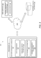
Fig 1 illustrates a diagram for a system for network bandwidth management, according to an example embodiment of the present disclosure. -
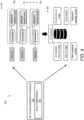
Fig 2 illustrates various components of a system for network bandwidth management, according to an example embodiment of the present disclosure. -
Fig. 3 illustrates various components of a system comprising a network bandwidth handler, a dynamic bandwidth allocator, and a load balancer used for network bandwidth management, according to another example embodiment of the present disclosure. -
Fig. 4 illustrates a pictorial representation of data harmonization by a data harmonizer deployed by a network bandwidth handler of a system for network bandwidth management, according to an example embodiment of the present disclosure. -
Fig. 5 illustrates a pictorial representation of collection of a time series distribution data by a data harmonizer, according to an example embodiment of the present disclosure. -
Fig. 6A illustrates a pictorial representation of an example of a trend data component of a time series distribution data, obtained by a baseline traffic estimator of a network bandwidth handler, according to an example embodiment of the present disclosure. -
Fig. 6B illustrates a pictorial representation of an example of a seasonal data component of a time series distribution data, obtained by a baseline traffic estimator, according to an example embodiment of the present disclosure. -
Fig. 6C illustrates a pictorial representation of an example of an irregular data component of a time series distribution data, identified by a baseline traffic estimator, according to an example embodiment of the present disclosure. -
Fig. 6D illustrates a pictorial representation of decomposition of a time series distribution data to obtain trend data component, seasonal data component, cyclic data component, and an irregular data component, by a baseline traffic estimator, according to an example embodiment of the present disclosure. -
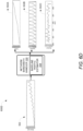
Fig. 7 illustrates a pictorial representation of computation of an auto regression data component and a moving average data component from an irregular data component by a lag parameter estimator of a network bandwidth handler, according to an example embodiment of the present disclosure. -
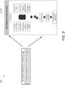
Fig. 8 illustrates a pictorial representation of estimation of bandwidth by a dynamic bandwidth estimator of a network bandwidth handler, according to an example embodiment of the present disclosure. -
Fig. 9 illustrates a pictorial representation of a plot representing a smooth polynomial curve constructed by a network bandwidth handler, in accordance with an example implementation of the present disclosure. -
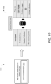
Fig. 10 illustrates a pictorial representation of data harmonization by a data harmonizer deployed by a network bandwidth handler, in an example use case, according to an example embodiment of the present disclosure. -
Fig. 11 illustrates a pictorial representation of baseline distribution traffic data computed by a network bandwidth handler, in an example use case, in accordance with an example embodiment of the present disclosure. -
Fig. 12 illustrates a pictorial representation of computation of an auto regression data component and a moving average data component from an irregular data component by a lag parameter estimator of a network bandwidth handler, in an example use case, according to an example embodiment of the present disclosure. -
Fig. 13 illustrates a pictorial representation of results indicating estimated network traffic computed by a network bandwidth handler, according to an example implementation of the present disclosure. -
Fig. 14 illustrates a pictorial representation of dynamic bandwidth allocation based on a bandwidth estimation, by a dynamic bandwidth allocator, according to an example embodiment of the present disclosure. -
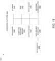
Fig. 15 illustrates a hardware platform for implementation of a system for network bandwidth management, according to an example embodiment of the present disclosure. -
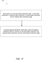
Figs. 16-21 illustrate process flowcharts for a system for network bandwidth management, according to an example embodiment of the present disclosure. - For simplicity and illustrative purposes, the present disclosure is described by referring mainly to examples thereof. The examples of the present disclosure described herein may be used together in different combinations. In the following description, details are set forth in order to provide an understanding of the present disclosure. It will be readily apparent, however, that the present disclosure may be practiced without limitation to all these details. Also, throughout the present disclosure, the terms "a" and "an" are intended to denote at least one of a particular element. The terms "a" and "an" may also denote more than one of a particular element. As used herein, the term "includes" means includes but not limited to, the term "including" means including but not limited to. The term "based on" means based at least in part on, the term "based upon" means based at least in part upon, and the term "such as" means such as but not limited to. The term "relevant" means closely connected or appropriate to what is being done or considered.
- Typically, bandwidth requirement of a server supporting a web service, such as, a website, a web page etc., can be expressed as a function of network traffic. Existing approaches for determining bandwidth requirement for a web server are based on forecasting network traffic for the future and by using several other factors such as, for example, the size of web pages provisioned by the web server, the computational capability of the web server supporting a web service, or the type of content on the web pages. Existing approaches for forecasting network traffic involve analyzing historical data i.e. past trend of network traffic or web demand by using various models such as, for example, a local trend model, a local seasonal model, or an intermittent demand model. Although existing approaches for network traffic forecasting involves analysis of historical network traffic, however, these approaches are usually based on certain assumptions. For instance, in some approaches, forecasting network traffic may not consider factors that may impact a portion of the network traffic, which cannot be defined in terms of any visible trend, pattern, seasonal or cyclic phase of usual traffic demand. Accordingly, network traffic estimation determined in such approaches may be inaccurate and may result in poor network bandwidth management, thereby causing server outages and loss of service by the server.
- The present disclosure describes a system, a method and a non-transitory computer readable medium for providing an estimated bandwidth according respectively to
independent claims - In some examples, the system includes various components, for example, a processor, a network bandwidth handler, a dynamic bandwidth allocator, and a load balancer to manage network bandwidth for the server. According to an example implementation of the present disclosure, the system may handle bandwidth of the server based on one or more operations performed by these components.
- A network bandwidth handler of the system accesses a time series distribution data including a distribution of data points. The distribution of data points, as referred herein, indicates an average count of network packets collected over a pre-defined time period. The average count of network packets is representative of network traffic at a server. In some examples, the pre-defined time period may be defined based on for instance, but not limited to, a user input, an application context, a business rule, etc. Furthermore, the network bandwidth handler determines, from the time series distribution data, one or more data components indicative of portions of network traffic contributed due to various factors. For instance, the network bandwidth handler decomposes the time series distribution data to determine data components like, a trend data component, a seasonal data component, a cyclical data component, and an irregular or residual data component, from the time series distribution data.
- The trend data component includes a distribution of a first set of data points indicative of a development or inherent trend of a first portion of the network traffic over the pre-defined time period. The seasonal data component includes a distribution of a second set of data points indicative of a second portion of the network traffic. The second set of data points is indicative of a recurring and persistent change in a pattern of the second portion of the network traffic. Likewise, the cyclical data component includes a distribution of a third set of data points indicative of a third portion of the network traffic developed due to a predefined operational rule. Furthermore, the irregular data component includes a fourth set of data points indicative of a fourth portion of the network traffic undefined by a definitive external factor.
- In accordance with said example implementation of the present disclosure, the network bandwidth handler computes a baseline distribution traffic data indicative of a base count of network packets over the pre-defined time period. The baseline distribution traffic data is computed based on the trend data component, the cyclical data component, and the seasonal data component..
- In an example, various traffic data components described herein may be influenced by a number of external factors, also referred herein as covariate metrics. The covariate metrics represents one or more external factors contributing to the network traffic over the pre-defined time period. For instance, in some examples, the covariate metrics may correspond to a size of a web page, a non-seasonal promotion, a count of images on the web page, a capability of the server hosting the web page, a load time interval for loading the web page, a ranking of the web page, a performance of a search optimizer coupled to the server, or other relevant factors.
- The network bandwidth handler may further identify from the irregular or residual data component, an auto regression data component and a moving average data component. The auto regression data component may correspond to a distribution of a fifth set of data points indicative of regression of the fourth set of data points over a lag time interval. Furthermore, the moving average data component may correspond to a distribution of a sixth set of data points indicative of regression of error values of the fourth set of data points over the lag time interval.
- Additionally, the network bandwidth handler determines an estimated network traffic for a future time interval based on the baseline distribution traffic data, a lagged covariate factor, and covariate metrics. The covariate metrics referred herein may correspond to other covariate factors for example, day part indicator, holiday indicator, etc. The lagged covariate factor may be determined based on the auto-regression data component and the moving average data component. The estimated network traffic may represent a forecast of expected network traffic in future. Furthermore, the network bandwidth handler may provide an estimated bandwidth for the future time interval based on a local weighted regression using a pre-defined smoothing parameter. The local weighted regression may be performed based on a local weighted scatter plot smoother model i.e. a LOESS model. In accordance with said example implementation of the present disclosure, the dynamic bandwidth allocator may allocate, network bandwidth to the server based on pre-stored network traffic data applicable for the server and the estimated bandwidth for the future time interval.
- Accordingly, the present disclosure aims to provide an accurate forecasting of network traffic that may be expected at a server at a future point in time. Accurately forecasting the network traffic for future enables efficient network bandwidth management for the server. For example, based on an expected network traffic, bandwidth requirements for the server may be pre-planned. Efficiently planning bandwidth requirements, such as an estimated bandwidth for the server to cater web demand in future helps in avoiding server outage or instances of crashing of server, due to unexpected increase in network traffic or the web demand. Also, by analyzing the forecasted network traffic and estimated bandwidth for the server, any instances of anticipated server failure may be identified, and preventive actions may be taken well in advance accordingly. In case of anticipated server failure, some of the preventive actions that may be taken may include, for example, deploying more servers to cater to increasing web demand, increasing computational capability of the servers, reducing load on the server, performing load balancing, improving data connection speed and/or quality of the server, reconfiguring network settings of the server, etc.
-
Fig. 1 illustrates asystem 100 for network bandwidth management, according to an example implementation of the present disclosure. In some examples, thesystem 100 may provide network bandwidth management for a server. The server may be for example, but not limited to, a web server or a server hosting a website or a web portal, and/or the like. Thesystem 100 may include aprocessor 120. Theprocessor 120 may be coupled to anetwork bandwidth handler 130, adynamic bandwidth allocator 140, and aload balancer 150. - The
network bandwidth handler 130 may correspond to a component that may handle bandwidth requirement for the server. For instance, according to an example, thenetwork bandwidth handler 130 may handle bandwidth requirement for the server based on changing network traffic conditions, over a period of time. Thenetwork bandwidth handler 130 may predict or forecast expected network traffic in future to identify bandwidth requirement for the server. According to an example, thenetwork bandwidth handler 130 may predict the expected network traffic by daypart, for instance, for different periods of a day, for example, morning, afternoon, or evening. In another example, thenetwork bandwidth handler 130 may predict the expected network traffic for any pre-defined time interval. Furthermore, based on the expected network traffic, thenetwork bandwidth handler 130 may provide an estimation of the bandwidth requirement for the server in the future i.e. for a future time instance. - The
dynamic bandwidth allocator 140 may allocate network bandwidth to the server based on one or more factors. For instance, in one example, thedynamic bandwidth allocator 140 may allocate network bandwidth to the server based on a current network traffic or web demand. In another example, thedynamic bandwidth allocator 140 may allocate the network bandwidth to the server based on the expected network traffic i.e. forecasted network traffic. Thedynamic bandwidth allocator 140 may access the expected network traffic from thenetwork bandwidth handler 130. Furthermore, in another example, thedynamic bandwidth allocator 140 may allocate the network bandwidth to the server based on the expected network traffic along with one or more of other factors for example, but not limited to, a size of web pages, computational capability of the server, a type of content developing the network traffic, a priority associated with the network traffic, a buffer bandwidth value, etc. In some examples, the bandwidth allocation for the server may be a function of size of web pages hosted by the server, the estimated network traffic, and a buffer value. In other examples, bandwidth allocation to the server may be performed based on load balancing of the network traffic. Theload balancer 150 of thesystem 100 may perform load balancing of the network traffic at the server. - The
load balancer 150 may monitor a current network traffic at the server and further perform load balancing of the network traffic at the server based on monitored traffic, under various situations. For example, in one situation, when a bandwidth allocated to the server is insufficient to support the current network traffic, theload balancer 150 may perform load balancing of the network traffic. Theload balancer 150 may perform a comparison of the allocated bandwidth to the server against a desired bandwidth based on the current network traffic. Accordingly, if the allocated bandwidth is determined to be less than the desired bandwidth, theload balancer 150 may perform the load balancing. In another example, theload balancer 150 may perform load balancing of the network traffic at several host servers based on current network traffic at the each of the several host servers and based on other factors. These factors may include, for example, expected network traffic, load history of the server, a type of content hosted by the server, etc. Further details of the load balancing by theload balancer 150 are described in reference toFigs 2 ,3 , and14 . - In accordance with an example implementation of the present disclosure, the
system 100 may perform bandwidth estimation for the server for a future point in time. Thenetwork bandwidth handler 130 may access time series distribution data. The time series distribution data may comprise a distribution of data points over a pre-defined time period. The time series distribution data may represent the distribution of data points i.e. data values corresponding to an average count of network packets over the pre-defined time period. The average count of network packets may be indicative of network traffic directed at a server during the pre-defined time period. The time series distribution data may be collected in a required or defined format for example, in a chronological order, so as to perform analysis and modelling of the time series distribution data to eventually forecast the expected network traffic, details of which are described hereinafter. - The
network bandwidth handler 130 may analyze the time series distribution data and identify one or more data components from the time series distribution data. Thenetwork bandwidth handler 130 may split or decompose the time series distribution data to obtain the various data components, based on an unobserved component model, which is described in further detail with reference toFigs. 2-21 . According to an example, the data components may be indicative of a distribution of one or more sets of data points collected over the pre-defined time period. Each set of the data points may represent a portion of the network traffic that may be developed at the server because of a key metric, details of which are described later in reference toFigs 2-21 . Thenetwork bandwidth handler 130 may determine from the time series distribution data, (a) a trend data component, (b) a seasonal data component, (c) a cyclical data component, and/or (d) a residual or irregular data component. Each of these data components may be expressed as a stochastic process that may include random variables which may evolve over the pre-defined time period. - The trend data component may include a first set of data points. The first set of data points may correspond to an inherent trend or development of network traffic over a pre-defined time period. The first set of data points corresponding to the trend data component may be indicative of development of a first portion of the network traffic. For instance, the trend data component may be indicative of a linearly or nonlinearly, increasing or decreasing trend of the network traffic, over the pre-defined time period.
Figs. 6A ,6D , and11 illustrates pictorial representation of examples of the trend data component. - Furthermore, the seasonal data component may include a distribution of second set of data points collected over the pre-defined time period. The second set of data points may be indicative of a second portion of the network traffic. The second portion of the network traffic may correspond to a recurring and/or persistent change in a pattern of development of the network traffic at the server. The recurring and/or persistent change may be due to seasonal factors. For instance, the seasonal data component may correspond to a portion of the network traffic on an e-commerce website hosted by the server due to a promotional offer running during a festival period.
Figs.6B ,6D , and11 illustrates pictorial representation of examples of the seasonal data component. - Furthermore, the cyclical data component may include a distribution of a third set of data points. The third set of data points may be indicative of a third portion of the network traffic. The third portion of the network traffic may be developed due to a predefined operational rule. For instance, the predefined operational rule may correspond to a business rule. The third portion of the network traffic at the server may be developed due to users visiting the e-commerce website during end of a business cycle or a financial quarter for the e-commerce business. The third portion of the network traffic may correspond to the cyclical data component.
- Accordingly, in accordance with various examples described herein, the
network bandwidth handler 130 may obtain, from the time series distribution data, one or more data components representative of stochastic processes that may be explained in terms of any pattern, behavior, or visible observation i.e. trend, seasonal phase, cyclic phase etc. from past traffic data i.e. historical network traffic data. For purpose of brevity, the trend data component, the seasonal data component, and the cyclic data component may be collectively referred hereinafter as explainable data components, hereinafter throughout the description. - Furthermore, in accordance with various examples, the
network bandwidth handler 130, upon identifying the explainable data components, may also identify a residual or left over data component. The residual or left over data component may be referred hereinafter as the irregular data component. The irregular data component may represent that portion of the network traffic that may not be explained in terms of any pattern, trend, or any visible behavior, in the historical network traffic data. The irregular data component may include a fourth set of data points collected over the pre-defined time period. The fourth set of data points may be indicative of a fourth portion of the network traffic. The fourth portion of the network traffic may correspond that portion of the network traffic which may be undefined or unexplained by a definitive external factor.Figs. 6C ,6D , and11 illustrates pictorial representation of examples of the irregular data component. - In accordance with an example implementation of the present disclosure, the
network bandwidth handler 130 may compute a baseline distribution traffic data. The baseline traffic data may be indicative of a base count of network packets over the pre-defined time period. Thenetwork bandwidth handler 130 may compute the baseline distribution traffic data based on the explainable data components, i.e. the trend data component, the seasonal data component, and the cyclic data component. Further details of computing the baseline distribution traffic data are described in reference toFigs. 2-21 . - According to an example implementation of the present disclosure, the
network bandwidth handler 130 may identify, from the irregular data component, an auto regression data component and a moving average data component. The auto regression data component may include a distribution of a fifth set of data points. The fifth set of data points may be indicative of regression of the fourth set of data points i.e. data points of the irregular data component over a lag time interval. Furthermore, the moving average data component may include a distribution of sixth set of data points. The sixth set of data points may be indicative of regression of error values of the fourth set of data points, over the lag time interval. In accordance with some examples, the identification of the auto regression data component and the moving average data component from the irregular data component, by thenetwork bandwidth handler 130, may provide a definitive explanation to unexplained portion of the network traffic collected in form of the time series distribution data. Said differently, identification of the auto regression data component and the moving average data component may provide an explanation to portion of the network traffic that may be left over after removing the explainable components. - The auto regression data component identified by the
network bandwidth handler 130 may be used to recognize a correlation between two data points of the fourth set of data points recorded at two different instances of time. The auto regression data component may provide a correlation between a first data point of the fourth set of data points with a second data point of the fourth set of data point. The second data point corresponds to a data value that may be recorded at a first time instance subsequent to a second time instance. A difference between data points at the first time instance and the second time instance, which are correlated may be referred as "lag time interval". The fifth set of data points i.e. data points corresponding to the auto regression data component may comprise such data points that may represent a regression of some data points of the fourth set of data points, over the lag time interval. - According to an example, to forecast the expected network traffic, along with computing the baseline distribution traffic data, the
network bandwidth handler 130 may identify the auto regression data component of the time series distribution data. Identification of the auto regression data component enables that an evolving variable of interest i.e. the fourth portion of the network traffic may be regressed upon its own lagged or prior values. Further details of the auto regression data component are described in reference toFigs 2-21 . - As stated earlier, the
network bandwidth handler 130 may identify the moving average data component from the irregular data component. The moving average data component may be used to recognize a correlation between error versions of two data points of the fourth set of data points at two different instances of time. For example, the moving average data component provides a correlation between a third data point of the fourth set of data points with a fourth data point of the fourth set of data point. The third data point and the fourth data point corresponds to error versions of respective data values recorded at two time instances. Said differently, the third data point represents an error version of an average count of network packets recorded at a third time interval and the fourth data point represents an error version of an average count of network packets that may be recorded at a fourth time interval. The fourth time interval may be subsequent to the third time interval. In other words, a difference between the fourth time interval and the third time interval may be referred as a second lag time interval. Thus, the sixth set of data points corresponding to the moving average data component may include data points representing regression of some error versions of data points of the fourth set of data points, over a lag time interval. In accordance with some examples, the identification of the moving average data component, by thenetwork bandwidth handler 130, enables that the unexplained portion i.e. the irregular data component holds a linear relationship with forecasted error terms. In other words, the data points corresponding to the sixth set lags upon previous error versions. Furthermore, based on the auto-regression data component and the moving average data component, thenetwork bandwidth handler 130 may determine the lagged covariate factor. The lagged covariate factor may be used along with other components, by thenetwork bandwidth handler 130, to estimate future network traffic. - In accordance with said example implementation, the
network bandwidth handler 130 may determine, an estimated network traffic for a future time point. Thenetwork bandwidth handler 130 may determine the estimated network traffic based on the data components computed by thenetwork bandwidth handler 130. For example, thenetwork bandwidth handler 130 may determine the estimated network traffic based on the baseline distribution traffic data, a lagged covariate factor, and covariate metrics. Thenetwork bandwidth handler 130 may perform a local weighted regression to determine the estimated network traffic. The local weighted regression may be performed using a LOESS model, which may utilize a smoothing parameter, further details of which are described later in reference toFigs. 2-21 . - Furthermore, the
network bandwidth handler 130 may provide an estimated bandwidth for the server for a future time period. Thenetwork bandwidth handler 130 may provide the estimated bandwidth for the server based on the estimated network traffic and/or other factors which are described in more details in description ofFigs. 2-21 . -
Fig 2 illustrates various components of thesystem 100 for network bandwidth management, according to an example implementation of the present disclosure. Thesystem 100 may include theprocessor 120. Theprocessor 120 may be coupled to thenetwork bandwidth handler 130, thedynamic bandwidth allocator 140, and theload balancer 150. The network bandwidth handler may include one or more components that may perform one or more operations for handling network bandwidth management for the server. For instance, thenetwork bandwidth handler 130 may include, for example, but not limited to, four units for (a) analyzing and processing historical network traffic data, (b) predicting an estimate of network traffic in future, and (c) providing an estimated bandwidth for the server. Thenetwork bandwidth handler 130 may include adata harmonizer 202, abaseline traffic estimator 204, alag parameter estimator 206, and adynamic bandwidth estimator 208. - The data harmonizer 202 may access a time
series distribution data 210. The timeseries distribution data 210 may include data points distributed over a pre-defined time period 212. The data points may correspond to data values indicating an average count of network packets directed at the server during the pre-defined time period 212. The data harmonizer 202 may access the timeseries distribution data 210 in a defined format. For instance, the data harmonizer 202 may access the timeseries distribution data 210 in a chronological order.Fig. 5 illustrates a pictorial representation of an example of the timeseries distribution data 210 that may be accessed by the data harmonizer 202 over the pre-defined time period 212. The timeseries distribution data 210 may represent a sequence of average count of network packets i.e. data points recorded at successive equally spaced time points of the pre-defined time period 212. In other words, according to an example, the timeseries distribution data 210 may correspond to a sequence of discrete-time data of historic instances of web traffic or network packets. - The pre-defined time period 212 may be a user defined time period. For example, a user may provide an input of a duration or range comprising a starting time and an ending time. Accordingly, the data harmonizer 202 may access the time
series distribution data 210 for the user defined time period. The timeseries distribution data 210 may represent a chronological representation of historical data of network traffic directed at the server. For example, the timeseries distribution data 210 may represent data points that may be aggregated thrice for each day i.e. Morning, Afternoon, and Evening. In one example, the timeseries distribution data 210 may represent historical data of network traffic at the server for past two years, and the data points indicating the average count of network packets would be distributed across 2190 instances of time i.e. 365*2*3. - The data harmonizer 202 may collect the time
series distribution data 210 that may include the distribution of data points representing portions of network traffic that may have been developed due to various external factors. For example, network traffic at a server hosting an e-commerce website may be affected due to various factors for example, but not limited to, a trending fashion or trending items, seasonal phases like festivals, wedding seasons, cyclical business rules like end of year sale, etc. In an aspect, various portions of the timeseries distribution data 210, i.e. past network traffic, may correspond to segments of thetime series data 210 that may be correlated to one or more of these factors. In other words, thecovariate metrics 214 may represent factors applicable at pre-defined time intervals of the pre-defined time period 212 for each segment of the timeseries distribution data 210. Thus, in some examples, data accessed by the data harmonizer 202 may be flagged or correlated with respect to one or more factors of thecovariate metrics 214. Thecovariate metrics 214 may be calculated by thenetwork bandwidth handler 130 based on the identification of one or more external factors influencing the network traffic over the pre-defined time period.Fig. 4 provides further details on the timeseries distribution data 210 aggregation based on thecovariate metrics 214. - In accordance with said example implementation of the present disclosure, the
network bandwidth handler 130 may include thebaseline traffic estimator 204. Thebaseline traffic estimator 204 may access the timeseries distribution data 210 from thedata harmonizer 202. Furthermore, thebaseline traffic estimator 204 may decompose the timeseries distribution data 210 into various data components. Thebaseline traffic estimator 204 may decompose the timeseries distribution data 210 to obtain atrend data component 216, aseasonal data component 218, acyclical data component 220, and anirregular data component 222. In accordance with some examples, the data components viz. thetrend data component 216, theseasonal data component 218, and thecyclic data component 220 may correspond to the explainable data components, as described earlier. Furthermore, these data components may be expressed as a stochastic process that include variables which may evolve over the pre-defined time period in a random manner. Following few paragraphs describes further details of each of these data components. - According to an example, the
trend data component 216 may include the first set of data points that may be indicative of development or inherent trend of a first portion of the network traffic. The first portion may be indicative of part of the network traffic that may be explained in form of a linear trend or a non-linear trend. For instance, thetrend data component 216 may include distribution of the first set of data points representing an overall increasing or a decreasing inherent trend of the network traffic developed over the pre-defined time period.Figs. 6A ,6D , and11 illustrates pictorial representation of examples of thetrend data component 216. Thebaseline traffic estimator 204 may identify thetrend data component 216 from the timeseries distribution data 210 using a random walk model, details of which are further described in reference toFigs.6A-6D and11 . - According to an example, the
seasonal data component 218 identified by thebaseline traffic estimator 204 may be indicative of a second portion of the network traffic developed over the pre-defined time period 212 due to a seasonal factor. Theseasonal data component 218 may include a distribution of second set of data points collected over the pre-defined time period. Data points of the second set of data points may represent such portions of the network traffic which may be developed in past due to a recurring event or a persistent or periodic change in usual events or a pattern of the network traffic. For example, the seasonal data component may represent portion of the network traffic at an e-commerce website hosted by the server that may be developed due to a festival offer e.g. Black Friday sale or New Year sale, or end of season sale or any other promotional offer, running during the pre-defined time period 212. In some examples, thebaseline traffic estimator 204 may identify theseasonal data component 218 based on deterministic seasonal trigonometric model, details of which are described further in reference toFigs. 2-21 . - The
cyclical data component 220 identified by thebaseline traffic estimator 204 may be indicative of the third portion of the network traffic at the server that may developed due to a predefined operational rule. The pre-defined operational rule referred herein, may correspond to a business rule, as described earlier in reference toFig. 1 . Thecyclic data component 220 may include a distribution of a third set of data points representative of the third portion of network traffic. For instance, in one example, the cyclic data component may correspond to the network traffic developed due to users visiting an online e-learning web portal hosted by the server, during start of an educational program or enrollment session of an e-learning module. - In accordance with some examples, the
baseline traffic estimator 204 may obtain, from the timeseries distribution data 210, data components viz. thetrend data component 216, theseasonal data component 218, thecyclic data component 220, and any other data component, that may be explained in terms of any pattern, behavior, or visible observation, from a previous history of network traffic or historical network traffic data i.e. the timeseries distribution data 210. Furthermore, thebaseline traffic estimator 204 may also identify a residual data component, i.e. anirregular data component 222 that may be unexplained in terms of previous history of network traffic or historical network traffic data, as described earlier. - The
irregular data component 222 may correspond to left over data components after splitting the explainable data components i.e. thetrend data component 216, theseasonal data component 218, thecyclic data component 220, from the timeseries distribution data 210. The fourth set of data points of the irregular data component may be indicative of a fourth portion of the network traffic undefined or unexplained by definitive external factor i.e. trend, pattern, seasonal phase, or cyclic phase.Figs. 6C ,6D , and11 illustrates pictorial representations of examples of theirregular data component 222. - In accordance with said example implementation of the present disclosure, the
baseline traffic estimator 204 may compute a baseline distribution traffic data. The baseline distribution traffic data may be indicative of an estimated baseline of distribution of the timeseries distribution data 210. Thebaseline traffic estimator 204 may compute the baseline distribution traffic data by forecasting an estimation of various sets of future data points corresponding to each of thetrend data component 216, theseasonal data component 218, and thecyclical data component 220. In an example, the baseline distribution traffic data may be expressed as a function of thetrend data component 216, theseasonal data component 218, and thecyclical data component 220.Fig. 11 illustrates a pictorial representation of an example of the baseline distribution traffic data computed by thebaseline traffic estimator 204. - In accordance with said example implementation of the present disclosure, the
lag parameter estimator 206 of thenetwork bandwidth handler 130 may perform estimation of theirregular data component 222 i.e. the unexplained data component of the timeseries distribution data 210. Thelag parameter estimator 206 may access theirregular data component 222 from thebaseline traffic estimator 204. Furthermore, thelag parameter estimator 206 may transform the data points of theirregular data component 222 as a weak stationary stochastic process. Thelag parameter estimator 206 may perform an evaluation to identify if one or more data points corresponding to theirregular data component 222 i.e. the fourth set of data points may be affected by its previous versions or any error versions of itself in past, details of which are described hereinafter. - The
lag parameter estimator 206 may determine an auto regression (AR)data component 224 and a movingaverage data component 226, from theirregular data component 222. TheAR data component 224 may include a distribution of a fifth set of data points. The fifth set of data points may be indicative of regression of the fourth set of data points of theirregular data component 222, over a first lag time interval. The first lag time interval for theAR data component 224 may be determined based on evaluation of a plot constructed using an auto-correlation function (ACF), by thelag parameter estimator 206, details of which are described later in the description. The ACF may be a function that may provide values of auto-correlation of a series, i.e., distribution of data points over a period of time with its lagged values. In other words, the auto-correlation function describes a relationship or a degree of relationship of present data values, i.e., data points with past data values, i.e. past data points. Furthermore, the movingaverage data component 226 may include a distribution of sixth set of data points. The sixth set of data points may be indicative of regression of error values of the fourth set of data points of theirregular data component 222, over a second lag time interval. The second lag time interval for the movingaverage data component 226 may be determined based on evaluation of a plot constructed using a partial auto-correlation function (PACF), details of which are described later in the description. The PACF may be a function that may provide values of partial-correlation of a series, i.e., a distribution of error versions of data points over a period of time with its lagged values. - The
lag parameter estimator 206 may identify theAR data component 224 to recognize a correlation between two data points of the fourth set of data points at two different instances of time separated by a lag interval. Said differently, by determining theAR data component 224, thelag parameter estimator 206, provides a correlation between a first data point of the fourth set of data points with a second data point of the fourth set of data point. The second data point corresponds to a data value that may be recorded subsequent to a lag time, i.e. after a time instance on which the first data point may be recorded. Accordingly, in one example, thelag parameter estimator 206 may identify all such data points from theirregular data component 222 that may be correlated with prior versions of itself. - The
lag parameter estimator 206 may establish that the second data point may be correlated with the first data point recorded at a previous instance of time, if the correlation between the two data points, exceeds a pre-defined threshold for example, a confidence threshold, details of which are further described in reference toFigs 7 and12 . Furthermore, thelag parameter estimator 206 may collate all such data points and respective time instances of recording of such data points as the fifth set of data points corresponding to theAR data component 224. In this manner, by the identification of theAR data component 224, thelag parameter estimator 206, may enable that some data points corresponding to the unexplainable part of the timeseries distribution data 210 may be explained as an evolving variable of interest i.e. data points regressed upon its own lagged or prior values. Furthermore, thelag parameter estimator 206 may estimate future values of such data points that may be considered for future network traffic forecasting by thenetwork bandwidth handler 130. - The
lag parameter estimator 206 may identify the movingaverage data component 226 to recognize a correlation between error versions of two data points of the fourth set of data points at two different instances of time. For instance, based on determination of the moving average component thelag parameter estimator 206, may provide a correlation between a third data point representative of an error value of the fourth set of data points with a fourth data point representative of another error value of the fourth set of data point. The fourth data point corresponds to a data value that may be recorded subsequent to a lag time, i.e. after a time instance on which the second data point may be recorded. Accordingly, thelag parameter estimator 206 may identify all such data points representing error versions of data values that may be correlated with prior error versions of itself. - In an example, similar to as described for the
AR data component 224, thelag parameter estimator 206 may establish that the fourth data point may be correlated with the third data point recorded at a previous instance of time, if the correlation between the two data points, exceeds a pre-defined threshold for example, a confidence threshold, details of which are further described in reference toFigs 7 and12 . Furthermore, thelag parameter estimator 206 may collate all such data points representing error versions of values at lagged time intervals and respective time instances of recording of such data points as the sixth set of data points corresponding to theAR data component 224. Furthermore, thelag parameter estimator 206 may estimate future error versions of data values that may be considered for future network traffic forecasting by thenetwork bandwidth handler 130. - In accordance with said example implementation, to determine the
AR data component 224 and the movingaverage data component 226, thelag parameter estimator 206, may compute afirst correlation parameter 228 and asecond correlation parameter 230, respectively. Furthermore, to estimate future data points i.e. data points for future time point corresponding to theirregular data component 222, thelag parameter estimator 206 may use thefirst correlation parameter 228 and thesecond correlation parameter 230, details of which are described in following paragraph. - The
lag parameter estimator 206 may construct, using the ACF, a first plot representing a distribution of correlation values between data points distributed over lagged time intervals. The first plot may include at least a first correlation value indicative of a first correlation between a part of network traffic at a first time instance and another part of the network traffic at a second time instance subsequent to the first time instance.Fig. 7 illustrates an example of pictorial representation of afirst plot 702 constructed by thelag parameter estimator 206. - The
lag parameter estimator 206 may construct, using the PACF, a second plot representing a distribution of correlation between error versions of data points over lagged time intervals. The second plot may include at least a second correlation value indicative of a second correlation between an error version of data point associated with a part of the network traffic at a third time instance and the error version of another data point associated another part of the network traffic at a fourth time instance. The fourth time instance may be subsequent to the third time instance.Fig. 7 also illustrates an example of pictorial representation of asecond plot 704 constructed by thelag parameter estimator 206. - Furthermore, the
lag parameter estimator 206 may determine, a first correlation parameter (P) 228 based on the first correlation value of the first plot and a first confidence threshold. Furthermore, thelag parameter estimator 206 may determine, a second correlation parameter (Q) 230 based on evaluation of the second correlation value of the second plot against a second confidence threshold. In accordance with various examples described herein, the first confidence threshold and the second confidence threshold may be pre-defined. In an example, these thresholds may be defined based on correlation series for different lagged values. For instance, a user may define these thresholds based on correlation trends present in the time series distribution data. Further, a factor that may influence these threshold may be auto-correlation itself. In an instance, the first confidence threshold and the second confidence threshold may be for example 95%. In another instance, the first confidence threshold and the second confidence threshold may be for example 90% and 85% respectively. - In accordance with an example, the first confidence threshold may be indicative of a threshold value beyond which any correlation value between two data points identified on the first plot may be considered as a high correlation. In other words, if the first correlation value on Y axis in the first plot is identified to be greater than or equal to the first confidence threshold, the
lag parameter estimator 206 may record a high correlation existing between two data points at a corresponding lag of the time interval on X axis. Accordingly, if the first correlation value on Y axis in the first plot is identified to be lesser than the first confidence threshold, thelag parameter estimator 206 may record a low correlation existing between two data points at a corresponding lag of the time interval on X axis. Similarly, the second confidence threshold may be indicative of a threshold value beyond which any correlation value between error versions of two data points identified on the second plot can be considered as a high correlation. In other words, if the second correlation value on Y axis in the second plot is identified to be greater than or equal to the second confidence threshold, thelag parameter estimator 206 may record a high correlation existing between error versions of two data points at a corresponding lag of the time interval on X axis. Accordingly, if the second correlation value on Y axis in the first plot is identified to be lesser than the second confidence threshold, thelag parameter estimator 206 may record a low correlation existing between error versions of two data points at a corresponding lag of the time interval on X axis. - In accordance with said example implementation, the
lag parameter estimator 206 may compute, theAR data component 224 based on the first correlation parameter (P) 228 for a future time instance and may compute the movingaverage data component 226 for the future time instance based on the second correlation parameter (Q) 230. Furthermore, a laggedcovariate factor 234 may be determined based on the AR data component and the movingaverage data component 226. Further details of theAR data component 224, the movingaverage data component 226, thefirst correlation parameter 228, and the secondcorrelation data parameter 230 are described in reference toFigs 7 and12 . - Moving to the
dynamic bandwidth estimator 208 component of thesystem 100, in accordance with an example implementation of the present disclosure, thenetwork bandwidth handler 130 may include thedynamic bandwidth estimator 208 to predict estimated network traffic for future time point. Furthermore, based on the estimated network traffic, thenetwork bandwidth handler 130 may provide abandwidth estimation 232 for the server. To determine the estimatedbandwidth 232, thedynamic bandwidth estimator 208 may utilize a LOESS i.e. a locally weighted scatter plotsmoother model 236 for predicting the estimated network traffic in future time point, details of which are described in following paragraph. - The
dynamic bandwidth estimator 208 may determine an estimated network traffic for a future time point based on multiple inputs. For instance, the estimated network traffic for the future time point may be determined based on (a) the baseline distribution traffic data, which is a combination oftrend data component 216,seasonal data component 218, and cyclical data component 220 (b) a laggedcovariate factor 234, and (c) thecovariate metrics 214. The laggedcovariate factor 234 may be computed by thedynamic bandwidth estimator 208 based on theAR data component 224 and/or the movingaverage data component 226 itself. Thedynamic bandwidth estimator 208 may provide, the baseline distribution traffic data, the laggedcovariate factor 234, and thecovariate metrics 214 as inputs to theLOESS model 236. Furthermore, based on output of theLOESS model 236, thedynamic bandwidth estimator 208 may determine the estimated network traffic for the future time point. Furthermore, thedynamic bandwidth estimator 208 may provide thebandwidth estimation 232 for the future time for the server based on the estimated network traffic for the future time point, details of which are further described in reference toFigs. 3-21 . - The
dynamic bandwidth allocator 140 may allocate network bandwidth to the server. Thedynamic bandwidth allocator 140 may allocate the network bandwidth dynamically to the server based on one or more factors and in different manners, which are described hereinafter, by way of several examples. For instance, in one example, thedynamic bandwidth allocator 140 may allocate network bandwidth to the server based on a networkbandwidth allocation data 238. The networkbandwidth allocation data 238 may include, for example, details of current bandwidth allocation to the server, bandwidth allocation details for the server at various past time intervals, etc. In another example, thedynamic bandwidth allocator 140 may allocate network bandwidth to the server based on other parameters likeweb server data 240 that may include data related to current network traffic or web demand. In another example, thedynamic bandwidth allocator 140 may allocate the network bandwidth to the server based on the estimated network bandwidth i.e. forecasted bandwidth accessed from thenetwork bandwidth handler 130. Furthermore, in some examples, thedynamic bandwidth allocator 140 may allocate the network bandwidth to the server based on thebandwidth estimation 232 along with other factors, for example, but not limited to, size of web pages, computational capability of the server, type of content developing the network traffic, priority associated with the network traffic or web demand, buffer bandwidth value, etc. The bandwidth allocation for the server, may be defined as a function of size of web pages hosted by the server, the estimated network traffic, and a buffer value. Accordingly, thedynamic bandwidth allocator 140 may compute the bandwidth and allocate it to the server. In another example, thedynamic bandwidth allocator 140 may allocate network bandwidth to the server based on network traffic data pre-stored as theweb server data 240 applicable for the server and/or thebandwidth estimation 232 for the future time point. - Moving to the
load balancer 150 component of thesystem 100, according to an example, theload balancer 150 may perform load balancing of the network traffic at the server. Theload balancer 150 may monitor a current network traffic at the server. Furthermore, theload balancer 150 may store data values of network traffic that may have been observed in recent time intervals. For instance, theload balancer 150 may store details corresponding to the network packets that may have been transacted at the server in recent past i.e. in a time period which may relatively far smaller than the pre-defined time period 212. Theload balancer 150 may store such data values ascurrent traffic data 242. Theload balancer 150 may store network traffic experienced in any pre-defined range of time period or user defined range of past time instances, ascurrent traffic data 242, and may use it for load balancing the network traffic at the server. The load balancer may analyze thecurrent traffic data 242 and perform load balancing of the network traffic at the server based on one or more pre-defined rules. For instance, in one example, theload balancer 150 may analyze thecurrent traffic data 242 to identify if the bandwidth allocated to the server is insufficient to support the current network traffic. Based on the identification, theload balancer 150 may perform load balancing of the network traffic at the server. In some examples, theload balancer 150 may perform a comparison of the allocated bandwidth to the server against a desired bandwidth based on thecurrent traffic data 242. Accordingly, theload balancer 150 may perform the load balancing, if the allocated bandwidth is determined to be less than the desired bandwidth. In some examples, the load balancing by theload balancer 150 may involve distributing, the current network traffic to several host servers based on pre-defined rules. The details pertaining to distribution of the network traffic performed by theload balancer 150 may be stored as traffic distribution data 244 and may be reused by theload balancer 150 on a future time instance. Said differently, theload balancer 150 may access the traffic distribution data 244 and may re-use a previously used traffic distribution schema stored in the traffic distribution data 244 for performing load balancing during a subsequent time instance. -
Fig. 3 illustrates various components of a system comprising thenetwork bandwidth handler 130, thedynamic bandwidth allocator 140, and theload balancer 150 used for network bandwidth management, according to another example implementation of the present disclosure. Illustratively, aweb service 302 may comprise thedynamic bandwidth allocator 140 and theload balancer 150 of thesystem 100, as described inFigs 1 and2 . Theweb service 302 may correspond to a cloud component, for example, a cloud based service or a cloud based infrastructure, or a cloud based platform. Thenetwork bandwidth handler 130 may be communicatively coupled to theweb service 302 via acommunication network 320. Furthermore, thenetwork bandwidth handler 130 and theweb service 302 may also be communicatively coupled to anetwork traffic database 304 via thecommunication network 320. Thenetwork traffic database 304 may store network traffic data at the plurality of servers during the pre-defined time period 212. - The
communication network 320 may be a cellular network, a broadband network, a telephonic network, an open network, such as the Internet, or a private network, such as an intranet and/or the extranet, or any combination thereof. In other examples, thecommunication network 320 can be any collection of distinct networks operating wholly or partially in conjunction to provide connectivity between thesystem 100, one or more servers, and/or the data source(s). Furthermore, the communication network 320 may include and/or support one or more networks, such as, but are not limited to, one or more of WiMax, a Local Area Network (LAN), Wireless Local Area Network (WLAN), a Personal area network (PAN), a Campus area network (CAN), a Metropolitan area network (MAN), a Wide area network (WAN), a Wireless wide area network (WWAN), or any broadband network, and may be further enabled with technologies such as, by way of example, Global System for Mobile Communications (GSM), Personal Communications Service (PCS), Bluetooth, WiFi, Fixed Wireless Data, 2G, 2.5G, 3G, 4G, IMT-Advanced, pre-4G, LTE Advanced, mobile WiMax, WiMax 2, WirelessMAN-Advanced networks, enhanced data rates for GSM evolution (EDGE), General packet radio service (GPRS), enhanced GPRS, iBurst, UMTS, HSPDA, HSUPA, HSPA, UMTS-TDD, 1×RTT, EV-DO, messaging protocols such as, TCP/IP, SMS, MMS, extensible messaging and presence protocol (XMPP), real time messaging protocol (RTMP), instant messaging and presence protocol (IMPP), instant messaging, USSD, IRC, or any other wireless data networks, broadband networks, or messaging protocols. - The
web service 302 may be coupled to a plurality of servers. Theload balancer 150 of theweb service 302 may monitor network traffic at the plurality of servers and perform load balancing of the network traffic at the plurality of servers, in a manner as described earlier in reference toFigs 1 and2 . Furthermore, theweb service 302 may access historical network traffic data from thenetwork traffic database 304 via thecommunication network 320. Thedynamic bandwidth allocator 140 may use the network traffic data accessed from thenetwork traffic database 304 and forecasted network traffic accessed from thenetwork bandwidth handler 130, to compute a network bandwidth to be allocated to a server. Thedynamic bandwidth allocator 140 may accordingly allocate the network bandwidth to the server.Fig. 14 illustrates a pictorial representation of an example of dynamic bandwidth allocation based on a bandwidth estimation, by a dynamic bandwidth allocator. -
Fig. 4 illustrates apictorial representation 400 of data harmonization by thedata harmonizer 202, according to an example implementation of the present disclosure. The data harmonizer 202 may be deployed by thenetwork bandwidth handler 130 of thesystem 100 for network bandwidth management. As illustrated in afirst view 402 of theFig. 4 , the data harmonizer 202 may access the timeseries distribution data 210. Illustratively, the timeseries distribution data 210 may include data points (D0-Dn) collected over a time period (T1-Tn). As described earlier in reference toFigs 1 and2 , the data points (D0-Dn) may represent an average count of network packets corresponding to network traffic that may be directed at a server at respective time instances of the time period (T1-Tn). The time period (T1-Tn) may correspond to the pre-defined time period 212 e.g. a user defined time period. The data harmonizer 202 may access the timeseries distribution data 210 in a defined format. For example, the data harmonizer 202 may access the timeseries distribution data 210 in a chronological order of day part time morning, afternoon, and evening. , These data points recorded at pre-defined time intervals may be arranged in a sequential order represented as a series of data values spread over the pre-defined time period. - The data points D0-Dn may be correlated with one or more external factors i.e. the
covariate metrics 214, as described earlier. Illustratively, the data points D0-Dn of the timeseries distribution data 210 may be correlated with covariates (Covariates t1, Covariates t2, ... Covariates Tn) relevant at respective time instances (T1-Tn). For example, D0 represents a data value indicating an average count of network packets developed due to covariates at time T1. Similarly, Dn represents a data value indicating an average count of network packets developed due to covariates at time Tn. As described earlier in reference toFigs. 1 and2 , one or more segments of the timeseries distribution data 210 may represent a distribution of various portions of network traffic which may have been developed due to various external factors. Said differently, each of the segments of the timeseries distribution data 210 may be correlated to one or more of these external factors. Various portions of the network traffic at the server may be impacted by the external factors, also referred herein as thecovariate metrics 214, influencing development of the network traffic or its any portion thereof at the server. Thecovariate metrics 214 for the timeseries distribution data 210 illustrated in theview 402, may be, clickable links on a web page of a web site hosted by the server, images on the web page, audio or video content on the web page, size of the web page, non-seasonal promotional offer on the web page, computational capability or speed of the server hosting the web page, etc. - Accordingly, the data harmonizer 202 may access the time
series distribution data 210 including average count of network packets based on thecovariate metrics 214 predominantly applicable at respective time instances (T1-Tn). Also, each data point of the distribution of data points in the timeseries distribution data 210 may be identified or flagged with one or more of thecovariate metrics 214, to which it may be correlated. As an example, referring to thefirst view 402, the data point D0 is associated with covariates at time instance T1. Similarly, the data point Dn is associated with covariates at time instance Tn, and so on. A second view 404 of theFig. 4 illustrates various external factors or thecovariate metrics 214 influencing the development of the network traffic corresponding to various portions of the timeseries distribution data 210. -
Fig. 5 illustrates apictorial representation 500 of collection of the timeseries distribution data 210 by thedata harmonizer 202, according to an example implementation of the present disclosure. The data harmonizer 202 may access the timeseries distribution data 210 in form of a plot i.e. a graph representing a data set. For example, as illustrated inFig. 5 , the data harmonizer 202 may access aplot 502 as an input. Theplot 502, as illustrated inFig. 5 , shows the distribution of data points (D0-Dn) distributed over the pre-defined time period ranging from time instance T0 to time instance Tn. Illustratively, value of each data point is represented onY axis 506 and time instance is represented onX axis 504. As an example, Dt represents value of data point i.e. average count of network packets at time instance t. Time period between time instance T0 to time instance Tn, as illustrated in theplot 502 may be a user defined time period. For example, a user may provide an input of a duration or range comprising a starting time T0 and an ending time Tn, for which the timeseries distribution data 210 may be accessed by thedata harmonizer 202. Accordingly, the data harmonizer 202 may access the timeseries distribution data 210 during the user defined time period. - Moving to
Fig. 6A , a pictorial representation of an example of thetrend data component 216 of the timeseries distribution data 210 is illustrated. Thetrend data component 216 may be obtained by thebaseline traffic estimator 204, according to an example embodiment of the present disclosure. According to an example, thebaseline traffic estimator 204 may access the timeseries distribution data 210. Furthermore, thebaseline traffic estimator 204 may decompose the timeseries distribution data 210 into one or more data components where each data component may be defined as a stochastic process. Accordingly, thebaseline traffic estimator 204 may obtain thetrend data component 216 from the timeseries distribution data 210. Furthermore, thebaseline traffic estimator 204 may also obtain other data components like theseasonal data component 218, thecyclic data component 220, and theirregular data component 222, details of which are described inFigs 6B onwards. -
Fig. 6A illustrates aplot 602A representing thetrend data component 216 of the timeseries distribution data 210. Thetrend data component 216 illustrated in theplot 602A represents the distribution of the first set of data points corresponding to an average count of network packets collected over the pre-defined time period (T0 - Tn). The first set of data points represented on theplot 602A may be indicative of such data points of the timeseries distribution data 210 that may correspond to an inherent development of the network traffic, for example, in form of a linearly increasingtrend 606A, over the pre-defined time period. Thus, theplot 602A of thetrend component data 216 represents a portion of the network traffic represented in theplot 502 of the timeseries distribution data 210. Illustratively, value of each data point of the first set of data points i.e. corresponding to thetrend data component 216 is represented on Y axis 604A and its corresponding time instance i.e. time instance of recording that data point is represented onX axis 504. - The
baseline traffic estimator 204 may obtain thetrend data component 216, as illustrated in theplot 602A, by using a random walk model. In a random walk model, for each time instance within the pre-defined time period 212, a variable may take a random step away from its previous value. The random walk model used for obtaining thetrend data component 216 from the timeseries data component 210 may be represented using an equation:
baseline traffic estimator 204 using the equation, as described above. -
Fig. 6B illustrates a pictorial representation of an example of theseasonal data component 218 of the timeseries distribution data 210, obtained by thebaseline traffic estimator 204. Thebaseline traffic estimator 204 may access the timeseries distribution data 210. Furthermore, thebaseline traffic estimator 204 may decompose the timeseries distribution data 210 to obtain theseasonal data component 218 from the timeseries distribution data 210.Fig. 6B illustrates aplot 602B representing theseasonal data component 218 of the timeseries distribution data 210. Theseasonal data component 218 as illustrated in theplot 602B represents the distribution of the second set of data points corresponding to an average count of network packets collected over the pre-defined time period (T0 - Tn). - The second set of data points represented on the plot 60BA may be indicative of such data points of the time
series distribution data 210 that may correspond to recurring and persistent change in a pattern of the development of the network traffic at the server. For instance, in some examples, a web server hosting a website for online purchase of air-conditioners and air coolers may experience more visits by users during months of summers. Accordingly, network traffic on such website may be high during a season and low during another season. Thus, theplot 602B of theseasonal data component 218 represents that portion of network traffic of the timeseries distribution data 210 that may be affected due to seasonality or a recurring pattern. Illustratively, in theplot 602B, a value of each data point of the second set of data points i.e. corresponding to theseasonal data component 218 is represented onY axis 604B, and its corresponding time instance i.e. time instance of recording that data point is represented onX axis 504. It may be observed that a recurring or persistent pattern indicating the seasonality or periodic characteristic of theseasonal data component 218 is noticeable in theplot 602B, after every Ta time interval. - The
baseline traffic estimator 204 may obtain theseasonal data component 218, as illustrated in theplot 602B, by using a deterministic trigonometric seasonal model. Using trigonometric seasonal model involves use of trigonometric functions. The trigonometric functions inherently includes seasonal or repeating pattern like structure, thereby, effectively capturing fluctuations in the data points of the timeseries distribution data 210 that may be impacted due to seasonal characteristics. In an example, the trigonometric seasonal model used for obtaining thetrend data component 216 from the timeseries distribution data 210 may be represented using the equation below: 2πt(i)/P- Ø)+ ε(i)
 may present a seasonality component, P represents a time period for which the seasonality reoccurs, i.e. duration after which seasonal pattern may be repeated, 'Ø' represents an unknown phase/shift parameter, which may impact the time period P, and 'I' represents an instance of time. Thus, each data point of the second set of data points for the pre-defined time period 212 and for any future time instance can be computed by the
baseline traffic estimator 204 using the equation, as described above. -
Fig. 6C illustrates a pictorial representation of an example of theirregular data component 222 obtained from the timeseries distribution data 210 by thebaseline traffic estimator 204, according to an example embodiment of the present disclosure. Aplot 602C representing theirregular data component 222 of the timeseries distribution data 210 is illustrated. Theplot 602C may represent a distribution of the fourth set of data points, i.e. the data points which may be left over after removing thetrend data component 216, theseasonal data component 218, and thecyclic data component 222 from the timeseries distribution data 210. The distribution of the fourth set of data points, as illustrated in the plot 602, may be representative of portions of the network traffic at the server that may be unexplained or undefined by definitive external factor i.e. trend, pattern, seasonal phase, or cyclic phase. -
Fig. 6D illustrates apictorial representation 600D of an example of decomposition of the timeseries distribution data 210, by thebaseline traffic estimator 204, to obtain thetrend data component 216, theseasonal data component 218, and theirregular data component 222 as described in reference toFigs 6A-6C . As illustrated in thepictorial representation 600D, the timeseries distribution data 210, represented by theplot 502, may be split into thetrend data component 216, represented by theplot 602A, the seasonal data component 218 (represented by theplot 602B), and theirregular data component 222, represented by theplot 602C, based on techniques as described earlier in reference toFigs. 6A-6C . -
Fig. 7 illustrates a pictorial representation of an example of computation of theAR data component 224 and the movingaverage data component 226, by thelag parameter estimator 206, according to an example embodiment of the present disclosure. As described earlier in reference toFig. 2 , thelag parameter estimator 206 may determine theAR data component 224 and the movingaverage data component 226 from theirregular data component 222. Illustratively, thelag parameter estimator 206 may access theplot 602C representing the distribution of the fourth set of data points corresponding to theirregular data component 222. Furthermore, thelag parameter estimator 206 may construct thefirst plot 702 and thesecond plot 704, in a similar manner, as described earlier in reference toFig. 2 . Thelag parameter estimator 206 may evaluate thefirst plot 702 and thesecond plot 704 to determine the first correlation parameter (P) 228 and the second correlation parameter (Q) 230. Thelag parameter estimator 206 may also compute theAR data component 224 and the movingaverage data component 226 using the first correlation parameter (P) 228 and the second correlation parameter (Q) 230. Thelag parameter estimator 206 may use the first correlation parameter (P) 228 and the second correlation parameter (Q) 230, to estimate future data points i.e. data points for future time point corresponding to theirregular data component 222. Thelag parameter estimator 206 may determine the fifth set of data points corresponding to theAR data component 224 and the sixth set of data points corresponding to the movingaverage data component 226. According to an example, the future data points identified in the fifth set of data points and the sixth set of data points may include such data points that may not have been captured in the baseline distribution traffic data computed by thebaseline traffic estimator 204. In other words, these sets of data points correspond to estimation of unexplained portion of the network traffic, as described earlier. - Referring to the
first plot 702 illustrated inFig. 7 , Y axis represents correlation values 706 and X axis representslag intervals 708. The correlation values 706 represented on Y axis may be indicative of a correlation between two data points of theirregular data component 222 at a given lag time interval. For example, as illustrated in theplot 702, at lag time interval '0', the correlation value on Y axis is '1'. Furthermore, at lag time interval `2', the correlation value is '-0.5' and at lag time interval `6' the correlation value is '-0.5'. Based on the evaluation of the correlation values 706 of thefirst plot 702, thelag parameter estimator 206 may identify that at lag time interval '0' there exists high correlation between two data points i.e. data points from amongst the fourth set of data points of theirregular data component 222. Similarly, thelag parameter estimator 206 may identify that at lag time intervals `2' and `6' there exists low correlation between two data points i.e. data points from amongst the fourth set of data points of theirregular data component 222. In a similar manner, thelag parameter estimator 206 may identify if two data points, from amongst the fourth set of data points, are highly correlated, moderately correlated, or not correlated at all. However, for estimating future data points corresponding to theAR data component 224 ofirregular data component 222, the lag parameter estimator, may only select lag interval values for the data points for which a correlation exceeds the first confidence threshold, as described earlier, inFig. 2 and further described hereinafter. - The
lag parameter estimator 206 may evaluate thefirst plot 702 to observe correlation values at various lag time intervals. For instance, thelag parameter estimator 702 may identify a correlation value of '1.0' at lag time interval '0'. The first correlation value may be indicative of a first correlation between a first data point y(t-Ig) representing the network traffic at a first time instance (t- Ig) and a second data point y (t) representing network traffic at a second time instance (t). The second time instance (t) may be a time instance occurring subsequently after a lag time interval 'Ig' to the first time instance (t-Ig). Here, 'Ig' represents a lag time interval represented on X axis of thefirst plot 702. - Furthermore, the
lag parameter estimator 206 may determine, the first correlation parameter (P) 228 based on comparison of the first correlation value and the first confidence threshold, as described earlier, in reference toFig. 2 . In accordance with various examples described herein, the first confidence threshold may correspond to pre-defined threshold value or may be a threshold value defined based on a user input. Illustratively, ahorizontal line 710 along the X axis represents the first confidence threshold. The first confidence threshold may be indicative of a threshold value beyond which any correlation value between two data points identified on thefirst plot 702 can be considered as a high correlation. In other words, if the first correlation value on Y axis in the first plot is identified to be greater than or equal to the first confidence threshold, thelag parameter estimator 206 may record a high correlation existing between two data points at a corresponding lag of the time interval on X axis. - The
lag parameter estimator 206 may evaluate thefirst plot 702 by comparing each correlation value at a respective lag interval against the first confidence threshold. Based on this comparison, the lag parameter may identify one or more lag intervals at which correlation between two data points is observed to be high i.e. correlation value is more than the first confidence threshold. For example, as illustrated in thefirst plot 702, the correlation value atlag time interval lag parameter estimator 206 may establish that there exists high correlation between two data points at a lag of `4'. Said differently, a first data point y (t) captured at point t may be highly correlated with the second data point y (t +4) captured at point t + 4. Accordingly, thelag parameter estimator 206 may use this information to determine the first correlation parameter (P) 228. - In accordance with various examples described herein, the first correlation parameter (P) represents a lag at which a regression happens at a data point on its prior values. Accordingly, the
lag parameter estimator 206 may compute theAR data component 224 using the first correlation parameter (P) 228. In other words, thelag parameter estimator 206 may compute data points corresponding to the fifth set of data points using the first correlation parameter (P) 228. Furthermore, as described earlier, the distribution of a fifth set of data points may be indicative of regression of the fourth set of data points over a first lag time interval i.e. a lag time interval at which high correlation exists between two data points. Furthermore, based on the computation of theAR data component 224, thelag parameter estimator 206 may estimate future data points corresponding to the irregular data component 122. - Referring to the
second plot 704, illustrated inFig. 7 , Y axis represents correlation values 712 and X axis representslag intervals 714. The correlation values 712 represented on Y axis may be indicative of a correlation between error versions of two data points of theirregular data component 222, at a defined lag time interval. For example, as illustrated in theplot 704, at lag time interval '0', the correlation value on Y axis is '-0.19'. Furthermore, at lag time interval `4', the correlation value is '0.2'. Thelag parameter estimator 206 may identify lag time intervals at which there exists high correlation, moderate correlation, or low correlation between error versions of two data points i.e. error versions of data points from amongst the fourth set of data points of theirregular data component 222, in a similar manner, as described for thefirst plot 702. However, for estimating future data points corresponding to the movingaverage data component 226 of theirregular data component 222, the lag parameter estimator, may only select lag interval values for the data points for which a correlation exceeds the second confidence threshold, as described inFig. 2 and further described hereinafter. - The
lag parameter estimator 206 may evaluate thesecond plot 704 to observe correlation values at various lag time intervals. The correlations value may be indicative of a first correlation between error version of a third data point z(t-Ig') representing the network traffic at a third time instance (t- Ig') and error version of a fourth data point z(t) representing network traffic at a fourth time instance (t). The fourth time instance (t) may be a time instance occurring subsequently after a lag time interval 'Ig" to the third time instance (t-Ig). Here, 'Ig" represents a lag time interval represented on X axis of thesecond plot 704. - Furthermore, the
lag parameter estimator 206 may determine, the second correlation parameter (Q) 230 based on comparison of the second correlation value and the second confidence threshold, as described earlier, in reference toFig. 2 . In accordance with various examples described herein, the second confidence threshold may correspond to pre-defined threshold value or may be a threshold value defined based on a user input. Illustratively,horizontal lines second plot 704 may be considered as a high correlation. In other words, if the first correlation value on Y axis in thesecond plot 704 is identified to be greater than or equal to the second confidence threshold, thelag parameter estimator 206 may record a high correlation existing between two data points at a corresponding lag of the time interval on X axis. - The
lag parameter estimator 206 may evaluate thesecond plot 704 by comparing each correlation value at a respective lag interval against the second confidence threshold. Based on this comparison, the lag parameter may identify one or more lag intervals at which correlation between error versions of the two data points is observed to be high i.e. correlation value is more than the first confidence threshold. Accordingly, in a similar manner, as described for thefirst plot 702, thelag parameter estimator 206 may use this information to determine the second correlation parameter (Q) 230. - In accordance with various examples described herein, the second correlation parameter (Q) represents a lag component at which a regression happens at error versions of a data point on its prior values. Accordingly, the
lag parameter estimator 206 may compute the movingaverage data component 226 using the second correlation parameter (Q) 230. Said differently, thelag parameter estimator 206 may compute data points corresponding to the sixth set of data points using the second correlation parameter (Q) 230. Furthermore, based on the computation of the movingaverage data component 226, thelag parameter estimator 206 may estimate future data points corresponding to the irregular data component 122. Accordingly, based on theAR data component 224 and the movingaverage data component 226, the lagged covariates, i.e., the laggedcovariate factor 234, may be determined. - In some examples, the
lag parameter estimator 206, may also determine a parameter 'D' indicative of a degree of differencing required to convert the timeseries distribution data 210 to a stationary time series. Thelag parameter estimator 206, may determine the parameter 'D' for instances where a time series processed by thelag parameter estimator 206 may not be stable. -
Fig. 8 illustrates apictorial representation 800 of estimation of bandwidth for the server, by thedynamic bandwidth estimator 208, according to an example embodiment of the present disclosure. Thedynamic bandwidth estimator 208, may determine an estimated network traffic for a future time point. Illustratively,view 802 depicts a pictorial representation of determination of estimated network traffic, by thedynamic bandwidth estimator 208. Thedynamic bandwidth estimator 208 may utilize a LOESS i.e. a locally weighted scatter plotsmoother model 236 to predict the estimated network traffic for the future time point and further determine the estimatedbandwidth 232 based on the estimated network traffic. Thedynamic bandwidth estimator 208 may compute one or more lagged variables based on the estimated parameters i.e. thefirst correlation parameter 228 and thesecond correlation parameter 230. - According to an example, the
dynamic bandwidth estimator 208 may determine the estimated network traffic for the future time point based on various components computed by thebaseline traffic estimator 204 and thelag parameter estimator 206. For instance, thedynamic bandwidth estimator 208 may determine the estimated network traffic for the future time point based on, the baseline distribution traffic data, thecovariate metrics 214, and the laggedcovariate factor 234. The laggedcovariate factor 234 may be computed by thedynamic bandwidth estimator 208 may compute based on theAR data component 224 and/or the movingaverage data component 226. The laggedcovariate factor 234 is indicative of lagged versions of one or more external covariate metrics i.e. thecovariate metrics 214, as described in reference toFig. 2 . - Furthermore, according to an example, the
dynamic bandwidth estimator 208 may provide a plurality of inputs to the LOESS model. For instance, as illustrated in theview 802, the inputs to the LOESS model may comprise one or more of: clickable links on a web page of a web site hosted by the server, images on the web page, audio or video content on the web page, size of the web page, non-seasonal promotional offer on the web page, computational capability or speed of the server hosting the web page, network packet count, self-lagged values, self-lagged error terms etc. Along with thesecovariate metrics 214, the inputs to the LOESS model may also comprise the baseline distribution traffic data, the laggedcovariate factor 234, and other such data. Thedynamic bandwidth estimator 208 may construct theLOESS model 236 on the inputs provided to theLOESS model 236. TheLOESS model 236 may be represent a local polynomial regression model. Thedynamic bandwidth estimator 208 may construct the LOESS model by performing a local weighted regression on the inputs. Thedynamic bandwidth estimator 208 may use the LOESS model based on a pre-defined smoothing parameter to construct a plot. The plot may represent a polynomial smooth curve that may fit between the network traffic and remaining covariates. Furthermore, in some examples, thedynamic bandwidth estimator 208 may utilize a polynomial equation as stated below for determining constructing the plot that fits the smooth curve:
- Accordingly, the
dynamic bandwidth estimator 208 may use the above equation used for constructing the plot i.e. the polynomial curve. An example of the polynomial curve that may be constructed by thedynamic bandwidth estimator 208 using the above equation is illustrated inFig. 9 . - In accordance with some example implementations of the present disclosure, performing the locally weighted smoothing regression may be best used in a context, when an underlying relationship of predictors and predicted variables may not seem to be following any certain pattern in the historical traffic data. In some examples, the external covariates used for determination of the estimated network traffic may be numerical or categorical. In some examples, the local regression technique of the LOESS model may involve locally fitting any function and providing an additional weight on each of the covariate depending on a likelihood with a point of interest.
-
Fig. 9 illustrates apictorial representation 900 of a plot 902 representing the smooth polynomial curve constructed by thedynamic bandwidth estimator 208 by using the LOESS model, in accordance with an example implementation of the present disclosure. In accordance with some examples, theLOESS model 236 may output the estimated network traffic for the future time point, as a function of various components like, the baseline traffic distribution, lagged covariates, external covariates etc. Thepolynomial curve 904, as illustrated inFig. 9 is representative of the afore-stated function. In other words, thepolynomial curve 904 is representative of a curve constructed by thedynamic bandwidth estimator 208 using the polynomial equation described earlier. - The
dynamic bandwidth estimator 208 may identify smaller segments time intervals onX axis 906, based on observed values of covariates. For instance, for a range (0>x<1000) illustrated onX axis 906 thedynamic bandwidth estimator 208 may identify smaller segments on theX axis 906 i.e. ranges 1-10, 10-20, 20-30, 30-50, 50-100... and so on. Furthermore, thedynamic bandwidth estimator 208 may fit data points using the polynomial equation, as described earlier for each of the identified segments. Furthermore, thedynamic bandwidth estimator 208 may integrate all such portions of small polynomial curves corresponding to the identified segments on theX axis 906 to construct a final curve, i.e. thepolynomial curve 904. Furthermore, thedynamic bandwidth estimator 208 may predict or forecast the estimated network traffic based on thepolynomial curve 904. - The
dynamic bandwidth estimator 208, based on output of theLOESS model 236, i.e. predicted network traffic for the future time point, may compute thebandwidth estimation 232 for the server and allocate the estimated bandwidth to the server, as described earlier in reference toFigs. 1 and2 . Thedynamic bandwidth estimator 208 may determine a minimum bandwidth requirement for the server based on multiplying the estimated network traffic for the future time to the size of web-pages hosted by the server. Furthermore, in some examples, thedynamic bandwidth estimator 208 may add a buffer value to the minimum bandwidth to determine thebandwidth estimation 232. Thebandwidth estimation 232 may be used by thedynamic bandwidth allocator 140 for allocating network bandwidth to the server. -
Figs. 10-13 illustrates pictorial representations of forecasting network traffic for future time point by thesystem 100 according to an example use case. The example use case referred herein relates to forecasting network traffic for a web server hosting a website of a food ordering application.Fig. 10 illustrates apictorial representation 1000 of data harmonization by thedata harmonizer 202, in an example use case, according to an example embodiment of the present disclosure. The data harmonizer 202 may access the timeseries distribution data 210 representing the network traffic at the website of food ordering application. The timeseries distribution data 210 accessed by the data harmonizer 202 may include data points D0-Dn indicating an average count of network packets corresponding to covariates relevant at respective time instances (T1-Tn) for the food ordering application. The data harmonizer 202 may collect the timeseries distribution data 210 in a defined format, for instance, in a chronological order of day part time i.e. morning, afternoon, and evening. These data points may be recorded at pre-defined time intervals and arranged in a sequential order to represent a distribution of data values over the pre-defined time period. - As described earlier in reference to
Fig. 2 , various portions or segments of the distribution of data points in the timeseries distribution data 210 may represent a distribution of various portions of network traffic that may have been developed due to various external factors. In this case, the external factors may correspond to factors applicable in context of the food ordering application. Thus, various portions of the network traffic represented as segments in the distribution of the timeseries distribution data 210 may be correlated to these external factors. An example of the external factors applicable for the afore-stated use case of the food ordering application is illustrated inview 1002. For example, the external factors influencing development of the network traffic or its any portion thereof at the web server hosting the food ordering application, may be, clickable links on a web page of a web site hosted by the server, images on the web page, audio or video content on the web page, size of the web page, non-seasonal promotional offer on the web page, computational capability or speed of the web server hosting the food ordering website, non-seasonal promotion, weekend indicator, holiday indicator, search engine optimization used for the web server, etc. As described earlier, these external factors may be represented as thecovariate metrics 214 predominantly applicable at pre-defined time intervals of the pre-defined time period. Thus, each data point of the distribution of data points in the timeseries distribution data 210 accessed by thedata harmonizer 202, may be identified or flagged with one or more of these external factors or thecovariate metrics 214, to which it may be correlated. -
Fig. 11 illustrates a pictorial representation of baseline distribution traffic data computed by thebaseline traffic estimator 204, in accordance with an example use case of the present disclosure. Thebaseline traffic estimator 204 may access the timeseries distribution data 210. The timeseries distribution data 210 may include a distribution of data points representative of the network traffic corresponding to the food ordering application on the server. In some examples, the timeseries distribution data 210 may represent pre-stored historical network traffic data that may be used in a training phase of constructing a model for forecasting network traffic.Fig. 11 illustrates anexample plot 1102 representing the timeseries distribution data 210 of the food ordering application. - Furthermore, as described earlier in reference to
Figs. 1 ,2 ,6A-6D , thebaseline traffic estimator 204 may decompose the timeseries distribution data 210, into various data components. For instance, thebaseline traffic estimator 204 may decompose the timeseries distribution data 210 to obtain thetrend data component 216, theseasonal data component 218, thecyclic data component 220, and theirregular data component 222. As described earlier, breaking the timeseries distribution data 210 into each of these data components that may be represented as unobserved stochastic processes which enables providing an explanation or definition to dynamic features of chronological series of the data points and a manner in which the data points change over time. -
Plots trend data component 216, theseasonal data component 218, and theirregular data component 222, respectively. Illustratively,plot 1104 representing thetrend data component 216 shows no increasing or decreasing trend. Furthermore, theplot 1106 representing distribution ofseasonal data component 218 shows dense distribution of data points in form of rectangular blocks. In an example, it may be because the data points corresponding to theseasonal data component 218 may be recorded at frequent time intervals. For example, seasonal data may be recorded daily for each day part i.e. morning, afternoon, and evening during the day. - The
baseline traffic estimator 204 may compute the baseline distribution traffic data, as described earlier in reference toFigs. 1 ,2 ,6A-6D . Thebaseline traffic estimator 204 may perform an estimation by extending values of thetrend data component 216 as represented in theplot 1102, theseasonal data component 218 as represented in theplot 1104 for a future time point, thereby constructing a baseline distribution. The baseline distribution traffic data may be indicative of a base count of network packets over the pre-defined time period.Plot 1110 illustrates the baseline distribution traffic data indicating a baseline of distribution of data points computed by thebaseline traffic estimator 204. - Illustratively, a
first distribution 1112 on theplot 1110 represents the baseline distribution traffic data computed by thebaseline traffic estimator 204 on thetime series data 210 i.e. theplot 1102. Furthermore, asecond distribution 1114 represents actual network traffic data that may have been observed for the pre-defined time period. Illustratively, thefirst distribution 1112 i.e. representing the baseline distribution traffic data overlaps some, but not all, portion of thesecond distribution 1114. Said differently, theplot 1110 illustrates a manner in which the baseline distribution traffic data i.e. thefirst distribution 1112 may vary with the actual time series distribution i.e. thesecond distribution 1114 accessed during the training phase. Therefore, a further analysis on theirregular component 222 of the timeseries distribution data 210 may be performed by thesystem 100 so as to match the estimation computed by thesystem 100 with actual observations of the network traffic data. -
Fig. 12 illustrates a pictorial representation of an example of computation of theAR data component 224 and the movingaverage data 226 component from theirregular data component 222 by thelag parameter estimator 206, according to the example use case of the food ordering application.Plot 1202 represents theirregular data component 222 obtained after the decomposition of the timeseries distribution data 210, as described inFig. 11 . Thelag parameter estimator 206 may express theirregular data component 222 as a weak stationary process. Thelag parameter estimator 206 may construct an auto-regressive moving average model that may provide a strict depiction of a weak stationary stochastic process in terms of polynomials viz. theAR data component 224 and the movingaverage data component 226. Furthermore, thelag parameter estimator 206 may identify theAR data component 224 and the movingaverage data component 226, from theirregular data component 222. - The
lag parameter estimator 206 may construct a plot 1204 using the ACF and aplot 1206 using the PACF, in a similar manner as described earlier inFig. 7 . Theplot 1206 may represent a distribution of correlation values between data points representing network traffic corresponding to the food ordering application, over lagged time intervals. Furthermore, the plot 106 may represent a distribution of correlation between error versions of the data points representing network traffic corresponding to the food ordering application, over lagged time intervals. Furthermore, thelag parameter estimator 206 may compute the first correlation parameter (P) 228 and the second correlation parameter (Q) 230, in a similar manner, as described earlier in reference toFig. 7 . For the afore-stated example use case, thelag parameter estimator 206 may compute the first correlation parameter (P) 228 as '1' and the second correlation parameter (Q) 230 as '0'. A value of the parameter 'D' indicative of a degree of differencing may be used as '0', as the timeseries distribution data 210 for the example use case is stationary in nature. -
Fig. 13 illustrates apictorial representation 1300 of results indicating estimated network traffic computed by thenetwork bandwidth handler 130, according to an example implementation of the present disclosure. Aplot 1302 ofFig. 13 illustrates a first series distribution indicating estimated network traffic computed by thenetwork bandwidth handler 130 for the pre-defined time period during a testing phase against an actual network traffic observed during the pre-defined time period.Illustratively X axis 1304 of theplot 1302 represents a time period starting from time instance T (0) to time instance T (n). Furthermore,Y axis 1306 of theplot 1302 represents an average count of network packets at the server. As illustrated, theplot 1302 includes two series distribution viz. afirst series distribution 1308 and asecond series distribution 1310. Thefirst series distribution 1308 may represent actual timeseries distribution data 210 that may have been observed at the server. Furthermore, thesecond series distribution 1310 represents an estimated time series distribution, i.e. expected network traffic computed by thenetwork bandwidth handler 130, computed during the testing phase, in accordance with the example implementation of the present disclosure. According to an example, the time period T (0) - T (n) may include a range corresponding to a future time interval. As illustrated in theplot 1302, there exists significant overlapping between thefirst series distribution 1308 and thesecond series distribution 1310. The overlapping of thefirst series distribution 1308 and thesecond series distribution 1310 may indicate that the estimated network traffic matches significantly with the actual network traffic observed at the server. - The
network bandwidth handler 130 may use the estimated network traffic i.e. thesecond series distribution 1310 to compute a bandwidth requirement for the server. Thenetwork bandwidth handler 130 may compute the bandwidth estimation based on techniques as described earlier in reference toFigs. 1 and2 . Thenetwork bandwidth handler 130 may identify from the estimated network traffic i.e. the secondtime series distribution 1310 that estimated forecasts for a next day are '47', '87', and '50'. Accordingly, thenetwork bandwidth handler 130 may compute the bandwidth estimation i.e. bandwidth requirement for future time point based on the estimated forecasts using techniques as described earlier in reference toFigs. 1 and2 . According to said example, thenetwork bandwidth handler 130 may compute a bandwidth requirement of the server for the next day as 100 MB in morning and evening, and 200MB for afternoon. In another example, thenetwork bandwidth handler 130 may identify from the estimated network traffic i.e. the secondtime series distribution 1310 that estimated forecasts for a day of a next month are '57', '130', and '74'. Accordingly, thenetwork bandwidth handler 130 may compute the bandwidth requirement of the server for the day of next month as 120 MB for morning, 275MB for afternoon, and 150MB for evening. Furthermore, in accordance with some examples, thedynamic bandwidth allocator 140 may access bandwidth requirement computed by thenetwork bandwidth handler 130 and accordingly, allocate network bandwidth to the server. -
Fig. 14 illustrates a pictorial representation of an example use case of dynamic bandwidth allocation based on forecasted traffic, by thedynamic bandwidth allocator 140 according to an example implementation of the present disclosure. Illustratively, aview 1402 depicts an example operation of network bandwidth management by thesystem 100. The network bandwidth operation, as illustrated in theview 1402, depicts steps of load balancing and dynamic bandwidth allocation at the server. - According to an example, a cloud computing based set up, for example, the
web service 304 as described inFig. 3 may include thedynamic bandwidth allocator 140 and theload balancer 150. As described earlier inFig. 3 , thedynamic bandwidth allocator 140 may manage bandwidth allocation for multiple servers. Furthermore, theload balancer 150 may perform load balancing of the network traffic at the multiple servers. The multiple servers referred herein may correspond to multiple host servers hosting one or more websites. In an example, separate spaces may be allocated to multiple web servers and data warehouses used in a business, by the web service. Furthermore, as illustrated in theview 1402, information from different sources may flow into a data warehouse including web servers, log servers, etc. The information may be indicative of current network traffic at multiple host servers. In one example, thesystem 100 may leverage information residing in the data warehouse and output it to the web server to accommodate the network traffic. - To perform load balancing, the
load balancer 150 may distribute the network traffic to the multiple servers. For example, theload balancer 150 may distribute the network traffic to different web hosts including a website. These hosts may have a pre-defined bandwidth. Furthermore, in an instance, when concurrent traffic flow is increased, theload balancer 150 may distribute the network traffic to multiple host servers. Theload balancer 150 may distribute the network traffic to multiple hosts servers based on techniques as described earlier, in reference toFigs. 1-3 . Theload balancer 150 may distribute the network traffic to different host servers based on pre-defined rules specific to an environment. - Furthermore, according to an example, the
system 100 may utilize time series data e.g. the timeseries distribution data 210 or historical network traffic data from the data warehouse to provide an early insight on future network traffic. For example, thenetwork bandwidth handler 130 may provide an estimation of the network traffic for future time point, in a similar manner as described in reference toFigs 1-13 . Furthermore, thedynamic bandwidth allocator 140 may use this information to dynamically allocate bandwidth to the multiple host servers. The bandwidth allocated to the host servers may suitably accommodate the concurrent traffic visiting the host servers or website hosted by the host servers. -
Fig. 15 illustrates ahardware platform 1500 for implementation of thesystem 100, according to an example embodiment of the present disclosure. Particularly, computing machines such as but not limited to internal/external server clusters, quantum computers, desktops, laptops, smartphones, tablets and wearables which may be used to execute thesystem 100 or may have the structure of thehardware platform 1500. Thehardware platform 1500 may include additional components not shown and that some of the components described may be removed and/or modified. In another example, a computer system with multiple GPUs can sit on external-cloud platforms including Amazon Web Services, or internal corporate cloud computing clusters, or organizational computing resources, etc. - Over
Fig. 15 , thehardware platform 1500 may be acomputer system 1500 that may be used with the examples described herein. Thecomputer system 1500 may represent a computational platform that includes components that may be in a server or another computer system. Thecomputer system 1500 may execute, by a processor e.g., a single or multiple processors or other hardware processing circuit, the methods, functions and other processes described herein. These methods, functions and other processes may be embodied as machine-readable instructions stored on a computer-readable medium, which may be non-transitory, such as hardware storage devices (e.g., RAM (random access memory), ROM (read-only memory), EPROM (erasable, programmable ROM), EEPROM (electrically erasable, programmable ROM), hard drives, and flash memory). Thecomputer system 1500 may include aprocessor 1505 that executes software instructions or code stored on a non-transitory computer-readable storage medium 1510 to perform methods of the present disclosure. The software code includes, for example, instructions to determine an estimated network traffic for a future time point for a server, provide an estimated bandwidth based on the estimated network traffic, and allocate network bandwidth dynamically based on the estimated bandwidth. Thenetwork bandwidth handler 130 i.e. comprising one or more of thedata harmonizer 202, thebaseline traffic estimator 204, thelag parameter estimator 206, thedynamic bandwidth estimator 208, thedynamic bandwidth allocator 140, and theload balancer 150 may be software codes or components performing these steps. - The instructions on the computer-
readable storage medium 1510 are read and stored the instructions instorage 1515 or in random access memory (RAM) 1520. Thestorage 1515 provides a large space for keeping static data where at least some instructions could be stored for later execution. The stored instructions may be further compiled to generate other representations of the instructions and dynamically stored in theRAM 1520. Theprocessor 1505 reads instructions from theRAM 1520 and performs actions as instructed. - The
computer system 1500 furthermore includes anoutput device 1525 to provide at least some of the results of the execution as output including, but not limited to, visual information to users, such as external agents. The output device can include a display on computing devices and virtual reality glasses. For example, the display can be a mobile phone screen or a laptop screen. GUIs and/or text are presented as an output on the display screen. Thecomputer system 1500 furthermore includesinput device 1530 to provide a user or another device with mechanisms for entering data and/or otherwise interact with thecomputer system 1500. Theinput device 1530 may include, for example, a keyboard, a keypad, a mouse, or a touchscreen. Theinput device 1530 may be used to provide an input of a time interval, for example, the pre-defined time period by a user. In an example, an output of any of thenetwork bandwidth handler 130, thedynamic bandwidth allocator 140, and theload balancer 150 may be displayed on theoutput device 1525. Each of theseoutput devices 1525 andinput devices 1530 could be joined by one or more additional peripherals. Theoutput device 1525 may be used to display an estimated bandwidth of the server. In another example, theoutput device 1525 may be used to display allocated network bandwidth to the server. In another example, theoutput device 1525 may be used to display a current network traffic at the server, and a load balancing performed by theload balancer 150 based on the current network traffic and the estimated bandwidth. - A
network communicator 1535 may be provided to connect thecomputer system 1500 to a network and in turn to other devices connected to the network including other clients, servers, data stores, and interfaces, for instance. Anetwork communicator 1535 may include, for example, a network adapter such as a LAN adapter or a wireless adapter. Thecomputer system 1500 includes adata source interface 1540 to accessdata source 1545. A data source is an information resource. As an example, a database of exceptions and rules may be a data source. Moreover, knowledge repositories and curated data may be other examples of data sources. -
Figs. 16-21 illustratesmethods system 100 for network bandwidth management, according to an example embodiment of the present disclosure. - It should be understood that method steps are shown here for reference only and other combinations of the steps may be possible. Furthermore, the methods 1600-2100 may contain some steps in addition to the steps shown in
Figs. 16-21 . For the sake of brevity, construction and operational features of thesystem 100 which are explained in detail in the description ofFigs. 1-15 are not explained in detail in the description ofFigs. 16-21 . The methods 1600-2100 may be performed by a component of thesystem 100, such as theprocessor 120, thenetwork bandwidth handler 130, thedynamic bandwidth allocator 140, and theload balancer 150. In some examples, one or more steps of the methods 1600-2100 may be performed by components such as, thedata harmonizer 202, thebaseline traffic estimator 204, thelag parameter estimator 206, and thedynamic bandwidth estimator 208 of thenetwork bandwidth handler 130. -
Fig. 16 illustrates a process flowchart of amethod 1600 for estimating bandwidth of a server by thesystem 100, in accordance with an example embodiment of the present disclosure. - At
block 1602, the timeseries distribution data 210 may be accessed. The timeseries distribution data 210 may comprise distribution of data points corresponding to an average count of network packets collected over a pre-defined time period. The average count of network packets, referred herein, may be representative of network traffic at a server at a given instance or time or a time interval. - In some examples, the time
series distribution data 210 may be representative of the distribution of the average count of network packets collected in a chronological order at pre-defined time intervals of the pre-defined time period. In some examples, the pre-defined time period may be defined by a user input or may be defined based on a business context or a pre- defined rule, for example, but not limited to, a business cycle, a quarter of a fiscal year, etc. Furthermore, in some examples, the timeseries distribution data 210 may also represent distribution of the average count of network packets corresponding to one or more portions of network traffic developed due to various covariate metrics, applicable at various time intervals, within the pre-defined time period. - At
block 1604, (i) thetrend data component 216, (ii) thecyclical data component 220, (iii) theseasonal data component 218, and (iv) the residual or theirregular data component 222 may be determined from the timeseries distribution data 210. Thetrend data component 216 may comprise a distribution of a first set of data points over the pre-defined time period 212. The first set of data points may be indicative of development or inherent trend of a first portion of the network traffic. Furthermore, theseasonal data component 218 may comprise a distribution of second set of data points. The second set of data points may be indicative of recurring and persistent change in a pattern of a second portion the network traffic over the pre-defined time period 212. Furthermore, thecyclical data component 220 may comprise distribution of a third set of data points. The third set of data points may be indicative of a third portion of the network traffic developed due to a predefined operational rule. Furthermore, theirregular data component 222 may comprise a fourth set of data points indicative of a fourth portion of the network traffic undefined by definitive external factor. - At
block 1606, a baseline distribution traffic data may be computed. The baseline distribution traffic data may be indicative of a base count of network packets over the pre-defined time period 212. The baseline distribution traffic data may be computed based on thetrend data component 216, thecyclical data component 220, and theseasonal data component 218. For instance, in some examples, the baseline distribution traffic data may be computed in a similar manner as described in reference toFigs. 1-14 . - Moving to block 1608, the
AR data component 224 and the movingaverage data component 226 may be identified from theirregular data component 222 to determine a lagged covariate factor. TheAR data component 224 may comprise a distribution of a fifth set of data points. The fifth set of data points may be indicative of regression of the fourth set of data points over a lag time interval. Furthermore, the movingaverage data component 226 may comprise a distribution of a sixth set of data points. The sixth set of data points may be indicative of regression of error values of the fourth set of data points over the lag time interval. According to some examples, theAR data component 224 may be computed in a similar manner as described in reference toFigs. 7 and12 . Furthermore, in some examples, the moving average data component may be computed in a similar manner as described in in reference toFigs. 7 and12 . At block 1610, an estimated network traffic for a future time interval may be determined. The estimated network traffic for the future time interval may be determined based on (a) a laggedcovariate factor 234, (b) the baseline distribution traffic data component and (c) the external covariates, i.e., thecovariate metrics 214. In an example, a local weighted regression on various key metrics and data points may be performed. For instance, the local weighted regression may be performed on inputs such as the baseline distribution traffic data, thecovariate metrics 214, and the laggedcovariate factor 234 using the LOESS model to determine the estimate network traffic for the future time point. - Furthermore, a LOESS model, as described in
Figs. 1-13 , may be constructed to determine the estimated network traffic based on the local weighted regression using a pre-defined smoothing parameter. The LOESS model may utilize thecovariate metrics 214, the baseline distribution traffic data component, and the laggedcovariate factor 234 computed from theAR data component 224, and the movingaverage data component 226, as inputs to construct a polynomial curve which may be used to identify data points corresponding to forecasted network traffic. - In some examples, the lagged
covariate factor 234 may correspond to covariate factors constructed based on modification to covariate factors existing in past over a lag time period. In some examples, the laggedcovariate factor 234 may be constructed based on theAR data component 224 and the movingaverage data component 226 as described earlier, in reference toFigs. 1-13 . - Moving to block 1612, the estimated bandwidth for the future time interval may be provided. The estimated bandwidth for the future time interval may be provided based on the estimated network traffic for the future time point. In some examples, the estimated bandwidth for the future time interval may be provided to dynamically allocate network bandwidth to the server to cater to a network traffic demand. Furthermore, the estimated bandwidth may be provided to configure network settings of the server.
- In some examples, the
method 1600 may further include one or more additional steps. For instance, in some examples, themethod 1600 may further accessing the estimated bandwidth, i.e. the estimated bandwidth provided at the block 1612. Furthermore, a network bandwidth may be allocated to the server based on the estimated bandwidth for the future time interval and based on pre-stored network traffic data applicable for the server at a given instance of time. Further details of these additional steps as indicated by branch labelled 'A' inFig. 16 are described in reference toFig. 20 . -
Fig. 17 illustrates a process flowchart of amethod 1700 for baseline traffic estimation from the timeseries distribution data 210 of network traffic, by thesystem 100, in accordance with an example embodiment of the present disclosure. - At
block 1702, the timeseries distribution data 210 may be decomposed to obtain (a) thetrend data component 216, (b) theseasonal data component 218, (c) thecyclic data component 220, and (d) theirregular data component 222. In some examples, the timeseries distribution data 210 may be decomposed in a similar manner as described in reference toFigs. 1-15 . - At
block 1704, upon decomposition of the timeseries distribution data 210, the baseline distribution traffic data may be computed. The baseline distribution traffic data may be a function of: thetrend data component 216, theseasonal data component 218, and thecyclical data component 220. -
Fig. 18 illustrates a process flowchart of amethod 1800 for computing a lagged covariate factor, by thesystem 100, in accordance with an example embodiment of the present disclosure. - At
block 1802, theirregular data component 222 may be accessed. Theirregular data component 222 may be obtained upon decomposition of the timeseries distribution data 210. In some examples, theirregular data component 222 may correspond to a residual data component of the timeseries distribution data 210. In other words, theirregular data component 222 may correspond to that portion of the network traffic which may be undefined by a definitive external factor. Theirregular data component 222 may correspond to the distribution that may include the fourth set of data points collected over the pre-defined time period 212, as described in reference toFigs. 1-15 . - At
block 1804, from theirregular data component 222, theAR data component 224 and the movingaverage data 226 component may be determined. TheAR data component 224 may be determined based on the auto-correlation function (ACF). Furthermore, the movingaverage data component 226 may be determined based on the partial auto-correlation function (PACF). The determination of theAR data component 224 and the movingaverage data 226 component may include additional steps. Further details of these additional steps as indicated by branch labelled 'B' inFig. 18 are described in reference toFig. 20 . - At
block 1806, a laggedcovariate factor 234 may be computed based on theAR data component 224 and the movingaverage data component 226. In some examples, the laggedcovariate factor 234 may be computed in a similar manner as described in reference toFigs. 1-15 . -
Fig. 19 illustrates a process flowchart of amethod 1900 for computing the auto regression data component and the moving average data component, by thesystem 100, in accordance with an example embodiment of the present disclosure. - At block 1902, a first plot may be constructed using an auto correlation function. The first plot may represent a distribution of a first correlation value. The first correlation value may be indicative of a first correlation between the network traffic at a first time instance and the network traffic at a second time instance subsequent to the first time instance. The
first plot 702, as illustrated inFig. 7 , is an example of the first plot that may be constructed at the block 1902. The first plot 1204, as illustrated inFig. 12 , is another example of the first plot that may be constructed at the block 1902. - At block 1904, a second plot may be constructed using a partial auto correlation function (PACF). The second plot may represent a distribution of a second correlation value. The second correlation value may be indicative of a partial auto correlation of network traffic residuals with itself at different lag values. In other words, the second correlation value indicates correlation between error versions associated with data points representing the network traffic at two different time instances. For example, the second correlation value may be indicative of correlation between an error version of a first data point representing network traffic at a third time instance and error version of a second data point representing network traffic at a fourth time instance subsequent to the third time instance. The
second plot 704 illustrated inFig. 7 is an example of the second plot that may be constructed at the block 1902. Thesecond plot 1206 illustrated inFig. 12 is another example of the second plot that may be constructed at the block 1904. - At
block 1906, a first correlation parameter may be determined. The first correlation parameter may be determined based on evaluation of the first correlation value of the first plot, against a first confidence threshold. The first correlation parameter may be determined in a similar manner as described earlier in reference toFigs. 1-15 . - At
block 1908, a second correlation parameter may be determined. The second correlation parameter may be determined based on evaluation of the second correlation value of the second plot, against a second confidence threshold. The second correlation parameter may be determined in a similar manner as described earlier in reference toFigs. 1-15 . - At
block 1910, a first lagged covariate value based on the ACF and a second lagged covariate value based on the PACF for a future time instance may be computed. In an example, the first lagged covariate value may be computed using the first correlation parameter and based on the ACF and the second lagged covariate may be computed using the second correlation parameter and based on the PACF. - Further, at
block 1912, the laggedcovariate factor 234 may be determined based on theAR data component 224 and the movingaverage data component 226. -
Fig. 20 illustrates a process flowchart of amethod 2000 for dynamically allocating network bandwidth by thesystem 100, in accordance with an example embodiment of the present disclosure. - At
block 2002, the estimated bandwidth may be accessed. , In some examples, thedynamic bandwidth allocator 140 may access the estimated bandwidth determined by thenetwork bandwidth handler 130. - At
block 2004, network bandwidth may be dynamically allocated to the server. The allocation of the network bandwidth may be based on pre-stored network traffic data applicable for the server and the estimated bandwidth for the future time interval accessed at theblock 2002. In some examples, the network bandwidth may be dynamically allocated in a similar manner, as described earlier, in reference toFigs. 1-15 . In some examples, themethod 2000 may include additional steps of load balancing. These additional steps as indicated by branch labelled 'C' inFig. 20 are described in reference toFig. 21 . -
Fig. 21 illustrates a process flowchart of a method 2100 for load balancing of the network traffic by thesystem 100, in accordance with an example embodiment of the present disclosure. - At
block 2102, the network traffic at the server may be monitored. In some examples, theload balancer 150 may monitor the network traffic at the server. - Moving to the
block 2104, a comparison between the network bandwidth allocated to the server against a desired network bandwidth i.e. network bandwidth required to support network traffic at a current time interval may be performed. In an instance, when the allocated network bandwidth to the server is less than the desired network bandwidth, the method moves to theblock 2106. However, in an instance, when the allocated network bandwidth to the server is more than the desired network bandwidth the method moves to theblock 2108. - At
block 2106, load balancing of the network traffic at the server may be performed. Theload balancer 130 may perform the load balancing of the server. In response to determination that the network bandwidth allocated to the server is insufficient to support the current network traffic, theload balancer 150 may offload some of the current network traffic to another server. In some examples, the load balancing may be performed in a similar manner as described in reference toFigs. 1-15 . - Furthermore, in some examples, the
load balancer 150 may notify thedynamic bandwidth allocator 140 and/or thenetwork bandwidth handler 130 about the load balancing performed at theblock 2106. For instance, theload balancer 150 may send a notification to thenetwork bandwidth allocator 130 to modify allocation of the network bandwidth to the server so as to support a current network traffic demand. In accordance with some examples, the load balancer may also notify thenetwork bandwidth handler 130 to take into consideration recent network traffic demanded at the server for estimation of the expected network traffic in near future. Thus, in some examples, thenetwork bandwidth handler 130 may recursively update bandwidth forecasting for the future time based on load balancing notification received from theload balancer 130 after performing the load balancing as described at theblock 2106. - At
block 2108, load balancing of the network traffic at the server may not be performed. In an instance, when at theblock 2104 it is determined that the network bandwidth allocated to the server may support the current network traffic, i.e. a current demand, no load balancing of the network traffic at the server may be performed. The server may continue to operate at the allocated network bandwidth until any further load balancing action is to be performed. - According to various examples described herein, the methods 1600-2100 may be practiced using a non-transitory computer-readable medium, for example, but not limited to the computer-
readable medium 1510 as described inFIG. 15 . In some examples, the methods 1600-2100 may be computer-implemented methods. - The present disclosure provides for the network bandwidth management. In some examples, the network bandwidth management may involve accurately forecasting or estimating an expected network traffic in future. Furthermore, in some examples, the network bandwidth management may involve efficient planning and dynamic allocation of the network bandwidth to one or more network entities, for example, but not limited to, servers, web server, web portals, online platforms, web services, web sites hosted by one or more servers, e-commerce platforms, and/or the like.
- One of ordinary skill in the art will appreciate that techniques consistent with the present disclosure are applicable in other contexts as well without departing from the scope of the disclosure. What has been described and illustrated herein are examples of the present disclosure. The terms, descriptions, and figures used herein are set forth by way of illustration only and are not meant as limitations. Many variations are possible within the scope of the following claims in which all terms are meant in their broadest reasonable sense unless otherwise indicated.
Claims (15)
- A system (100; 1500) comprising:a processor (120; 1505); anda network bandwidth handler (130) coupled to the processor, the network bandwidth handler configured to:access time series distribution data (210) comprising a distribution of data points corresponding to an average count of network packets over a pre-defined time period, wherein the average count of network packets is representative of network traffic at a server;determine from the time series distribution data:a trend data component (216) comprising a distribution of a first set of data points indicative of an inherent trend of a first portion of the network traffic over the pre-defined time period,a seasonal data component (218) comprising distribution of a second set of data points indicative of recurring and persistent change in a pattern of a second portion of the network traffic over the pre-defined time period,a cyclical data component (220) comprising distribution of a third set of data points indicative of a third portion of the network traffic developed due to a predefined operational rule, andan irregular data component (222) comprising a fourth set of data points indicative of a fourth portion of the network traffic undefined by a definitive external factor;compute baseline distribution traffic data indicative of a base count of network packets over the pre-defined time period, based on the trend data component, the cyclical data component, and the seasonal data component;determine, using a local weighted regression, an estimated network traffic for a future time interval based on the baseline distribution traffic data, a lagged covariate factor (234), and covariate metrics (214), wherein the covariate metrics represent one or more external factors contributing to the network traffic over the pre-defined time period, and wherein the lagged covariate factor is indicative of lagged versions of one or more of the covariate metrics; andprovide an estimated bandwidth (232) for the future time interval based on the estimated network traffic to configure network settings of the server, the configuration of network settings including configuring at least one of a file and print service settings, file transfer settings, domain name server, DNS, settings, remote access settings, web service settings, email settings, and dynamic host configuration protocol, DHCP settings.
- The system as claimed in claim 1 further comprising:
a dynamic bandwidth allocator (140) coupled to the processor, the dynamic bandwidth allocator configured to allocate network bandwidth to the server based on pre-stored network traffic data applicable for the server and the estimated bandwidth for the future time interval. - The system as claimed in claim 1 or 2, further comprising:
a load balancer (150) coupled to the processor, the load balancer configured to:monitor current network traffic (242) at the server; andperform load balancing of the current network traffic at the server by distributing a portion of the current network traffic to a remote server, when an allocated network bandwidth is less than a desired network bandwidth to support the current network traffic. - The system as claimed in any previous claim, wherein:the network bandwidth handler comprises a data harmonizer (202) coupled to the processor, the data harmonizer configured to collect the time series distribution data in a chronological order representing a distribution of the average count of network packets corresponding to the covariate metrics, at pre-defined time intervals of the pre-defined time period; and/orwherein the network bandwidth handler is configured to calculate the covariate metrics based on identifying external factors influencing the network traffic at an instance of time, and wherein the covariate metrics comprise at least one of: a size of a web page, a non-seasonal promotion, a count of images on the web page, a capability of the server, a load time interval for loading the web page, a ranking of the web page, and a performance of a search optimizer coupled to the server.
- The system as claimed in any previous claim, wherein the network bandwidth handler comprises:
a baseline traffic estimator (204) coupled to the processor, the baseline traffic estimator configured to:decompose the time series distribution data to obtain the trend data component, the seasonal data component, the cyclical data component, and the irregular data component; andcompute the baseline distribution traffic data, wherein the baseline distribution traffic data is a function of the trend data component, the seasonal data component, and the cyclical data component. - The system as claimed in any previous claim, wherein the network bandwidth handler comprises a dynamic bandwidth estimator (208) coupled to the processor, the dynamic bandwidth estimator configured to compute the lagged covariate factor based on an auto regression data component (224) and a moving average data component (226), determined from the irregular data component, and wherein:the auto regression data component comprises a distribution of a fifth set of data points indicative of regression of the fourth set of data points over a first lag time interval; andthe moving average data component comprises a distribution of a sixth set of data points indicative of regression of error values of the fourth set of data points over a second lag time interval.
- The system as claimed in claim 6, wherein the network bandwidth handler comprises a lag parameter estimator (206) coupled to the processor, the lag parameter estimator configured to:access the irregular data component of the time series distribution data; anddetermine from the irregular data component, the auto regression data component based on an auto-correlation function, ACF, and the moving average data component based on a partial auto-correlation function, PACF.
- The system as claimed in claim 7, wherein the lag parameter estimator is configured to:construct using the ACF, a first plot (702) representing a distribution of a first correlation value indicative of a first correlation between the network traffic at a first time instance and the network traffic at a second time instance subsequent to the first time instance;construct using the PACF, a second plot (704) representing a distribution of a second correlation value indicative of a second correlation between an error version associated with the network traffic at a third time instance and the error version associated with network traffic at a fourth time instance subsequent to the third time instance;determine a first correlation parameter (228) based on the first correlation value of the first plot and a first confidence threshold (710; 711);determine a second correlation parameter (230) based on evaluation of the second correlation value of the second plot against a second confidence threshold (716; 718); andcompute the auto regression data component based on the first correlation parameter for a future time instance and the moving average data component for the future time instance based on the second correlation parameter.
- A method comprising:accessing, by a processor (120; 1505) coupled to a network bandwidth handler, a dynamic bandwidth allocator and a load balancer, time series distribution data (210) comprising distribution of data points corresponding to an average count of network packets over a pre-defined time period, wherein the average count of network packets is representative of network traffic at a server;determining, by the processor, from the time series distribution data,a trend data component (216) comprising distribution of a first set of data points indicative of an inherent trend of a first portion of the network traffic over the pre-defined time period,a seasonal data component (218) comprising distribution of a second set of data points indicative of recurring and persistent change in a pattern of a second portion of the network traffic over the pre-defined time period,a cyclical data component (220) comprising distribution of a third set of data points indicative of a third portion of the network traffic developed due to a predefined operational rule, andan irregular data component (222) comprising a fourth set of data points indicative of a fourth portion of the network traffic undefined by definitive external factor;computing, by the processor, a baseline distribution traffic data indicative of a base count of network packets over the pre-defied time period, based on the trend data component, the cyclical data component, and the seasonal data component;determining, using a local weighted regression, an estimated network traffic for a future time interval based on the baseline distribution traffic data, a lagged covariate factor (234), and covariate metrics (214), wherein the covariate metrics represent one or more external factors contributing to the network traffic over the pre-defined time period, and wherein the lagged covariate factor is indicative of lagged versions of one or more of the covariate metrics; andproviding an estimated bandwidth (232) for the future time interval based on the estimated network traffic for the future time interval to configure network settings of the server, the configuration of network settings including configuring at least one of a file and print service settings, file transfer settings, domain name server, DNS, settings, remote access settings, web service settings, email settings, and dynamic host configuration protocol, DHCP, settings.
- The method as claimed in claim 9, further comprising:allocating, by the processor, network bandwidth to the server based on pre-stored network traffic data applicable for the server and the estimated bandwidth for the future time interval; and/ormonitoring, by the processor, current network traffic (242) at the server; andperforming, by the processor, load balancing of the current network traffic at the server by distributing a portion of the current network traffic to a remote server, when an allocated network bandwidth is less than a desired network bandwidth to support the current network traffic.
- The method as claimed in claim 9 or 10, further comprising:collecting, by the processor, the time series distribution data in a chronological order representing a distribution of the average count of network packets corresponding to the covariate metric at pre-defined time intervals of the pre-defined time period; and/ordecomposing, by the processor, the time series distribution data to obtain, the trend data component, the seasonal data component, the cyclical data component, and the irregular data component; andcomputing, by the processor, the baseline distribution traffic data, wherein the baseline distribution traffic data is a function of: the trend data component, the seasonal data component, and the cyclical data component.
- The method of any of claims 9 to 11, wherein providing the estimated bandwidth comprises computing, by the processor, the lagged covariate factor based on an auto regression data component (224) and a moving average data component (226) determined from the irregular data component, and wherein:the auto regression data component comprises a distribution of a fifth set of data points indicative of regression of the fourth set of data points over a lag time interval, andthe moving average data component comprises a distribution of a sixth set of data points indicative of regression of error values of the fourth set of data points over the lag time interval.
- The method as claimed in claim 12, further comprising:accessing, by the processor, the irregular data component of the time series distribution data; anddetermining, by the processor, from the irregular data component, the auto regression data component based on an auto-correlation function, ACF, and the moving average data component based on a partial auto-correlation function, PACF.
- The method of claim 13, wherein determining the auto regression data component and the moving average data component further comprises:constructing, by the processor, using the ACF, a first plot (702) representing distribution of a first correlation value indicative of a first correlation between the network traffic at a first time instance and the network traffic at a second time instance subsequent to the first time instance;constructing, by the processor, using the PACF, a second plot (704) representing distribution of a second correlation value indicative of a second correlation between error version associated with the network traffic at a third time instance and the error version associated with network traffic at a fourth time instance subsequent to the third time instance;determining, by the processor, a first correlation parameter (228) based on evaluation of the first correlation value of the first plot, against a first confidence threshold (710; 711);determining, by the processor, a second correlation parameter (230) based on evaluation of the second correlation value of the second plot against a second confidence threshold (716; 718); andcomputing, by the processor, the auto regression data component based on the first correlation parameter for a future time instance and the moving average data component for the future time instance based on the second correlation parameter.
- A non-transitory computer readable medium (1510) including machine readable instructions that are executable by a processor (120; 1505) to perform, at least, the method as claimed in at least one of claims 9 to 14.
Applications Claiming Priority (1)
| Application Number | Priority Date | Filing Date | Title |
|---|---|---|---|
| US16/808,865 US11316743B2 (en) | 2020-03-04 | 2020-03-04 | Network bandwidth management |
Publications (2)
| Publication Number | Publication Date |
|---|---|
| EP3876476A1 EP3876476A1 (en) | 2021-09-08 |
| EP3876476B1 true EP3876476B1 (en) | 2023-08-30 |
Family
ID=74556775
Family Applications (1)
| Application Number | Title | Priority Date | Filing Date |
|---|---|---|---|
| EP21155523.0A Active EP3876476B1 (en) | 2020-03-04 | 2021-02-05 | Network bandwidth management |
Country Status (2)
| Country | Link |
|---|---|
| US (1) | US11316743B2 (en) |
| EP (1) | EP3876476B1 (en) |
Families Citing this family (4)
| Publication number | Priority date | Publication date | Assignee | Title |
|---|---|---|---|---|
| US20220138642A1 (en) * | 2020-11-03 | 2022-05-05 | At&T Intellectual Property I, L.P. | Forecasting based on planning data |
| US11979325B2 (en) * | 2021-01-28 | 2024-05-07 | VMware LLC | Dynamic SD-WAN hub cluster scaling with machine learning |
| US11601478B2 (en) * | 2021-06-29 | 2023-03-07 | Microsoft Technology Licensing, Llc | Media server management for communication session |
| US20230394085A1 (en) * | 2022-06-07 | 2023-12-07 | HCL America Inc. | Method and system for analyzing and interacting with centralized telecommunication networks through multi-layer graphs |
Family Cites Families (10)
| Publication number | Priority date | Publication date | Assignee | Title |
|---|---|---|---|---|
| US7251589B1 (en) | 2005-05-09 | 2007-07-31 | Sas Institute Inc. | Computer-implemented system and method for generating forecasts |
| US8010394B2 (en) * | 2007-11-28 | 2011-08-30 | Yahoo! Inc. | System and method to facilitate yearly inventory forecasting for network-based entities |
| US20090198559A1 (en) | 2008-02-06 | 2009-08-06 | Disney Enterprises, Inc. | Multi-resolutional forecasting system |
| KR101012863B1 (en) * | 2008-09-25 | 2011-02-08 | 한국전력공사 | Load forecasting analysis system for generation of customer baseline load |
| US10713578B2 (en) | 2015-04-29 | 2020-07-14 | Cisco Technology, Inc. | Estimating utilization of network resources using time series data |
| US10476949B2 (en) * | 2017-02-21 | 2019-11-12 | Microsoft Technology Licensing, Llc | Predictive autoscaling in computing systems |
| US10387900B2 (en) * | 2017-04-17 | 2019-08-20 | DataRobot, Inc. | Methods and apparatus for self-adaptive time series forecasting engine |
| US10635565B2 (en) | 2017-10-04 | 2020-04-28 | Servicenow, Inc. | Systems and methods for robust anomaly detection |
| EP3804226A1 (en) * | 2018-06-06 | 2021-04-14 | The Joan and Irwin Jacobs Technion-Cornell Institute | Telecommunications network traffic metrics evaluation and prediction |
| US11620528B2 (en) * | 2018-06-12 | 2023-04-04 | Ciena Corporation | Pattern detection in time-series data |
-
2020
- 2020-03-04 US US16/808,865 patent/US11316743B2/en active Active
-
2021
- 2021-02-05 EP EP21155523.0A patent/EP3876476B1/en active Active
Also Published As
| Publication number | Publication date |
|---|---|
| EP3876476A1 (en) | 2021-09-08 |
| US20210281486A1 (en) | 2021-09-09 |
| US11316743B2 (en) | 2022-04-26 |
Similar Documents
| Publication | Publication Date | Title |
|---|---|---|
| EP3876476B1 (en) | Network bandwidth management | |
| US11320469B2 (en) | Systems and methods for processing different data types | |
| US10210036B2 (en) | Time series metric data modeling and prediction | |
| Garg et al. | A framework for ranking of cloud computing services | |
| US9137130B2 (en) | Dynamic network load forecasting | |
| US11153176B2 (en) | Exponential moving maximum (EMM) filter for predictive analytics in network reporting | |
| US10783002B1 (en) | Cost determination of a service call | |
| US20150244645A1 (en) | Intelligent infrastructure capacity management | |
| US10909503B1 (en) | Snapshots to train prediction models and improve workflow execution | |
| US10628766B2 (en) | Method and system for enabling dynamic capacity planning | |
| Balaji et al. | Predictive Cloud resource management framework for enterprise workloads | |
| Grosskop et al. | Identification of application-level energy optimizations | |
| Kumar et al. | Performance assessment of time series forecasting models for cloud datacenter networks’ workload prediction | |
| US11310125B2 (en) | AI-enabled adaptive TCA thresholding for SLA assurance | |
| US20210263718A1 (en) | Generating predictive metrics for virtualized deployments | |
| US20180218468A1 (en) | Mentor-protégé matching system and method | |
| Efimov et al. | Integration data model for continuous service delivery in cloud computing system | |
| CN104937613A (en) | Heuristics to quantify data quality | |
| Kanagaraj et al. | Uniform distribution elephant herding optimization (UDEHO) based virtual machine consolidation for energy-efficient cloud data centres | |
| Marques et al. | Proactive resource management for cloud of services environments | |
| US20150371257A1 (en) | Systems and methods for predicting results based on marketing data | |
| Coppolino et al. | Effective QoS monitoring in large scale social networks | |
| US20170154276A1 (en) | Event prediction system and method | |
| McCreadie et al. | Leveraging data-driven infrastructure management to facilitate AIOps for big data applications and operations | |
| US20230418598A1 (en) | Modernizing application components to reduce energy consumption |
Legal Events
| Date | Code | Title | Description |
|---|---|---|---|
| PUAI | Public reference made under article 153(3) epc to a published international application that has entered the european phase |
Free format text: ORIGINAL CODE: 0009012 |
|
| STAA | Information on the status of an ep patent application or granted ep patent |
Free format text: STATUS: THE APPLICATION HAS BEEN PUBLISHED |
|
| AK | Designated contracting states |
Kind code of ref document: A1 Designated state(s): AL AT BE BG CH CY CZ DE DK EE ES FI FR GB GR HR HU IE IS IT LI LT LU LV MC MK MT NL NO PL PT RO RS SE SI SK SM TR |
|
| STAA | Information on the status of an ep patent application or granted ep patent |
Free format text: STATUS: REQUEST FOR EXAMINATION WAS MADE |
|
| 17P | Request for examination filed |
Effective date: 20220308 |
|
| RBV | Designated contracting states (corrected) |
Designated state(s): AL AT BE BG CH CY CZ DE DK EE ES FI FR GB GR HR HU IE IS IT LI LT LU LV MC MK MT NL NO PL PT RO RS SE SI SK SM TR |
|
| REG | Reference to a national code |
Ref country code: DE Ref legal event code: R079 Ref document number: 602021004585 Country of ref document: DE Free format text: PREVIOUS MAIN CLASS: H04L0012240000 Ipc: H04L0041089600 Ref country code: DE Ref legal event code: R079 Ipc: H04L0041089600 |
|
| GRAP | Despatch of communication of intention to grant a patent |
Free format text: ORIGINAL CODE: EPIDOSNIGR1 |
|
| STAA | Information on the status of an ep patent application or granted ep patent |
Free format text: STATUS: GRANT OF PATENT IS INTENDED |
|
| RIC1 | Information provided on ipc code assigned before grant |
Ipc: H04L 43/026 20220101ALN20230227BHEP Ipc: H04L 41/147 20220101ALN20230227BHEP Ipc: H04L 41/142 20220101ALN20230227BHEP Ipc: H04L 41/0823 20220101ALN20230227BHEP Ipc: H04L 41/0273 20220101ALN20230227BHEP Ipc: H04L 67/101 20220101ALI20230227BHEP Ipc: H04L 47/70 20220101ALI20230227BHEP Ipc: H04L 47/125 20220101ALI20230227BHEP Ipc: H04L 47/122 20220101ALI20230227BHEP Ipc: H04L 43/0876 20220101ALI20230227BHEP Ipc: H04L 43/04 20220101ALI20230227BHEP Ipc: H04L 41/0896 20220101AFI20230227BHEP |
|
| INTG | Intention to grant announced |
Effective date: 20230330 |
|
| RIC1 | Information provided on ipc code assigned before grant |
Ipc: H04L 43/026 20220101ALN20230320BHEP Ipc: H04L 41/147 20220101ALN20230320BHEP Ipc: H04L 41/142 20220101ALN20230320BHEP Ipc: H04L 41/0823 20220101ALN20230320BHEP Ipc: H04L 41/0273 20220101ALN20230320BHEP Ipc: H04L 67/101 20220101ALI20230320BHEP Ipc: H04L 47/70 20220101ALI20230320BHEP Ipc: H04L 47/125 20220101ALI20230320BHEP Ipc: H04L 47/122 20220101ALI20230320BHEP Ipc: H04L 43/0876 20220101ALI20230320BHEP Ipc: H04L 43/04 20220101ALI20230320BHEP Ipc: H04L 41/0896 20220101AFI20230320BHEP |
|
| GRAS | Grant fee paid |
Free format text: ORIGINAL CODE: EPIDOSNIGR3 |
|
| GRAA | (expected) grant |
Free format text: ORIGINAL CODE: 0009210 |
|
| STAA | Information on the status of an ep patent application or granted ep patent |
Free format text: STATUS: THE PATENT HAS BEEN GRANTED |
|
| AK | Designated contracting states |
Kind code of ref document: B1 Designated state(s): AL AT BE BG CH CY CZ DE DK EE ES FI FR GB GR HR HU IE IS IT LI LT LU LV MC MK MT NL NO PL PT RO RS SE SI SK SM TR |
|
| P01 | Opt-out of the competence of the unified patent court (upc) registered |
Effective date: 20230720 |
|
| REG | Reference to a national code |
Ref country code: GB Ref legal event code: FG4D |
|
| REG | Reference to a national code |
Ref country code: CH Ref legal event code: EP |
|
| REG | Reference to a national code |
Ref country code: DE Ref legal event code: R096 Ref document number: 602021004585 Country of ref document: DE |
|
| REG | Reference to a national code |
Ref country code: IE Ref legal event code: FG4D |
|
| REG | Reference to a national code |
Ref country code: LT Ref legal event code: MG9D |
|
| REG | Reference to a national code |
Ref country code: NL Ref legal event code: MP Effective date: 20230830 |
|
| REG | Reference to a national code |
Ref country code: AT Ref legal event code: MK05 Ref document number: 1606880 Country of ref document: AT Kind code of ref document: T Effective date: 20230830 |
|
| PG25 | Lapsed in a contracting state [announced via postgrant information from national office to epo] |
Ref country code: GR Free format text: LAPSE BECAUSE OF FAILURE TO SUBMIT A TRANSLATION OF THE DESCRIPTION OR TO PAY THE FEE WITHIN THE PRESCRIBED TIME-LIMIT Effective date: 20231201 |
|
| PG25 | Lapsed in a contracting state [announced via postgrant information from national office to epo] |
Ref country code: IS Free format text: LAPSE BECAUSE OF FAILURE TO SUBMIT A TRANSLATION OF THE DESCRIPTION OR TO PAY THE FEE WITHIN THE PRESCRIBED TIME-LIMIT Effective date: 20231230 |
|
| PG25 | Lapsed in a contracting state [announced via postgrant information from national office to epo] |
Ref country code: SE Free format text: LAPSE BECAUSE OF FAILURE TO SUBMIT A TRANSLATION OF THE DESCRIPTION OR TO PAY THE FEE WITHIN THE PRESCRIBED TIME-LIMIT Effective date: 20230830 Ref country code: RS Free format text: LAPSE BECAUSE OF FAILURE TO SUBMIT A TRANSLATION OF THE DESCRIPTION OR TO PAY THE FEE WITHIN THE PRESCRIBED TIME-LIMIT Effective date: 20230830 Ref country code: NO Free format text: LAPSE BECAUSE OF FAILURE TO SUBMIT A TRANSLATION OF THE DESCRIPTION OR TO PAY THE FEE WITHIN THE PRESCRIBED TIME-LIMIT Effective date: 20231130 Ref country code: LV Free format text: LAPSE BECAUSE OF FAILURE TO SUBMIT A TRANSLATION OF THE DESCRIPTION OR TO PAY THE FEE WITHIN THE PRESCRIBED TIME-LIMIT Effective date: 20230830 Ref country code: LT Free format text: LAPSE BECAUSE OF FAILURE TO SUBMIT A TRANSLATION OF THE DESCRIPTION OR TO PAY THE FEE WITHIN THE PRESCRIBED TIME-LIMIT Effective date: 20230830 Ref country code: IS Free format text: LAPSE BECAUSE OF FAILURE TO SUBMIT A TRANSLATION OF THE DESCRIPTION OR TO PAY THE FEE WITHIN THE PRESCRIBED TIME-LIMIT Effective date: 20231230 Ref country code: HR Free format text: LAPSE BECAUSE OF FAILURE TO SUBMIT A TRANSLATION OF THE DESCRIPTION OR TO PAY THE FEE WITHIN THE PRESCRIBED TIME-LIMIT Effective date: 20230830 Ref country code: GR Free format text: LAPSE BECAUSE OF FAILURE TO SUBMIT A TRANSLATION OF THE DESCRIPTION OR TO PAY THE FEE WITHIN THE PRESCRIBED TIME-LIMIT Effective date: 20231201 Ref country code: FI Free format text: LAPSE BECAUSE OF FAILURE TO SUBMIT A TRANSLATION OF THE DESCRIPTION OR TO PAY THE FEE WITHIN THE PRESCRIBED TIME-LIMIT Effective date: 20230830 Ref country code: AT Free format text: LAPSE BECAUSE OF FAILURE TO SUBMIT A TRANSLATION OF THE DESCRIPTION OR TO PAY THE FEE WITHIN THE PRESCRIBED TIME-LIMIT Effective date: 20230830 |
|
| PGFP | Annual fee paid to national office [announced via postgrant information from national office to epo] |
Ref country code: IE Payment date: 20231211 Year of fee payment: 4 Ref country code: FR Payment date: 20231212 Year of fee payment: 4 |
|
| PG25 | Lapsed in a contracting state [announced via postgrant information from national office to epo] |
Ref country code: PL Free format text: LAPSE BECAUSE OF FAILURE TO SUBMIT A TRANSLATION OF THE DESCRIPTION OR TO PAY THE FEE WITHIN THE PRESCRIBED TIME-LIMIT Effective date: 20230830 Ref country code: NL Free format text: LAPSE BECAUSE OF FAILURE TO SUBMIT A TRANSLATION OF THE DESCRIPTION OR TO PAY THE FEE WITHIN THE PRESCRIBED TIME-LIMIT Effective date: 20230830 |
|
| PG25 | Lapsed in a contracting state [announced via postgrant information from national office to epo] |
Ref country code: ES Free format text: LAPSE BECAUSE OF FAILURE TO SUBMIT A TRANSLATION OF THE DESCRIPTION OR TO PAY THE FEE WITHIN THE PRESCRIBED TIME-LIMIT Effective date: 20230830 |
|
| PG25 | Lapsed in a contracting state [announced via postgrant information from national office to epo] |
Ref country code: SM Free format text: LAPSE BECAUSE OF FAILURE TO SUBMIT A TRANSLATION OF THE DESCRIPTION OR TO PAY THE FEE WITHIN THE PRESCRIBED TIME-LIMIT Effective date: 20230830 Ref country code: RO Free format text: LAPSE BECAUSE OF FAILURE TO SUBMIT A TRANSLATION OF THE DESCRIPTION OR TO PAY THE FEE WITHIN THE PRESCRIBED TIME-LIMIT Effective date: 20230830 Ref country code: ES Free format text: LAPSE BECAUSE OF FAILURE TO SUBMIT A TRANSLATION OF THE DESCRIPTION OR TO PAY THE FEE WITHIN THE PRESCRIBED TIME-LIMIT Effective date: 20230830 Ref country code: EE Free format text: LAPSE BECAUSE OF FAILURE TO SUBMIT A TRANSLATION OF THE DESCRIPTION OR TO PAY THE FEE WITHIN THE PRESCRIBED TIME-LIMIT Effective date: 20230830 Ref country code: DK Free format text: LAPSE BECAUSE OF FAILURE TO SUBMIT A TRANSLATION OF THE DESCRIPTION OR TO PAY THE FEE WITHIN THE PRESCRIBED TIME-LIMIT Effective date: 20230830 Ref country code: CZ Free format text: LAPSE BECAUSE OF FAILURE TO SUBMIT A TRANSLATION OF THE DESCRIPTION OR TO PAY THE FEE WITHIN THE PRESCRIBED TIME-LIMIT Effective date: 20230830 Ref country code: PT Free format text: LAPSE BECAUSE OF FAILURE TO SUBMIT A TRANSLATION OF THE DESCRIPTION OR TO PAY THE FEE WITHIN THE PRESCRIBED TIME-LIMIT Effective date: 20240102 Ref country code: SK Free format text: LAPSE BECAUSE OF FAILURE TO SUBMIT A TRANSLATION OF THE DESCRIPTION OR TO PAY THE FEE WITHIN THE PRESCRIBED TIME-LIMIT Effective date: 20230830 |
|
| PGFP | Annual fee paid to national office [announced via postgrant information from national office to epo] |
Ref country code: DE Payment date: 20231212 Year of fee payment: 4 |