EP3629246B1 - Systems and methods for neural architecture search - Google Patents
Systems and methods for neural architecture search Download PDFInfo
- Publication number
- EP3629246B1 EP3629246B1 EP19154841.1A EP19154841A EP3629246B1 EP 3629246 B1 EP3629246 B1 EP 3629246B1 EP 19154841 A EP19154841 A EP 19154841A EP 3629246 B1 EP3629246 B1 EP 3629246B1
- Authority
- EP
- European Patent Office
- Prior art keywords
- model
- weightings
- candidate
- candidate model
- models
- Prior art date
- Legal status (The legal status is an assumption and is not a legal conclusion. Google has not performed a legal analysis and makes no representation as to the accuracy of the status listed.)
- Active
Links
- 238000000034 method Methods 0.000 title claims description 59
- 230000001537 neural effect Effects 0.000 title claims description 18
- 230000006870 function Effects 0.000 claims description 85
- 238000013528 artificial neural network Methods 0.000 claims description 73
- 238000012549 training Methods 0.000 claims description 71
- 210000002569 neuron Anatomy 0.000 claims description 30
- 230000008569 process Effects 0.000 claims description 17
- 238000012360 testing method Methods 0.000 claims description 15
- 238000004458 analytical method Methods 0.000 claims description 14
- 238000010200 validation analysis Methods 0.000 claims description 11
- 230000002787 reinforcement Effects 0.000 claims description 9
- 238000004590 computer program Methods 0.000 claims description 5
- 230000001419 dependent effect Effects 0.000 claims description 2
- 230000009471 action Effects 0.000 description 11
- 239000011159 matrix material Substances 0.000 description 11
- 238000007476 Maximum Likelihood Methods 0.000 description 9
- 238000010586 diagram Methods 0.000 description 8
- 238000012545 processing Methods 0.000 description 5
- 230000000306 recurrent effect Effects 0.000 description 5
- 239000003795 chemical substances by application Substances 0.000 description 4
- 230000004044 response Effects 0.000 description 4
- 230000009286 beneficial effect Effects 0.000 description 3
- 238000004891 communication Methods 0.000 description 3
- 238000012804 iterative process Methods 0.000 description 3
- 238000013459 approach Methods 0.000 description 2
- 238000003491 array Methods 0.000 description 2
- 230000000694 effects Effects 0.000 description 2
- 238000011156 evaluation Methods 0.000 description 2
- 230000006872 improvement Effects 0.000 description 2
- 238000005457 optimization Methods 0.000 description 2
- 238000005192 partition Methods 0.000 description 2
- 230000009467 reduction Effects 0.000 description 2
- 238000005070 sampling Methods 0.000 description 2
- 238000013519 translation Methods 0.000 description 2
- 230000004913 activation Effects 0.000 description 1
- 230000008901 benefit Effects 0.000 description 1
- 239000002775 capsule Substances 0.000 description 1
- 230000008859 change Effects 0.000 description 1
- 238000006243 chemical reaction Methods 0.000 description 1
- 230000000052 comparative effect Effects 0.000 description 1
- 238000007596 consolidation process Methods 0.000 description 1
- 239000000470 constituent Substances 0.000 description 1
- 238000013527 convolutional neural network Methods 0.000 description 1
- 238000013500 data storage Methods 0.000 description 1
- 230000007423 decrease Effects 0.000 description 1
- 238000001514 detection method Methods 0.000 description 1
- 230000003993 interaction Effects 0.000 description 1
- 238000012886 linear function Methods 0.000 description 1
- 238000010801 machine learning Methods 0.000 description 1
- 230000000717 retained effect Effects 0.000 description 1
- 230000008054 signal transmission Effects 0.000 description 1
- 230000036962 time dependent Effects 0.000 description 1
- 238000012876 topography Methods 0.000 description 1
Images

Classifications
-
- G—PHYSICS
- G06—COMPUTING; CALCULATING OR COUNTING
- G06N—COMPUTING ARRANGEMENTS BASED ON SPECIFIC COMPUTATIONAL MODELS
- G06N3/00—Computing arrangements based on biological models
- G06N3/02—Neural networks
- G06N3/08—Learning methods
-
- G—PHYSICS
- G06—COMPUTING; CALCULATING OR COUNTING
- G06N—COMPUTING ARRANGEMENTS BASED ON SPECIFIC COMPUTATIONAL MODELS
- G06N3/00—Computing arrangements based on biological models
- G06N3/02—Neural networks
- G06N3/08—Learning methods
- G06N3/086—Learning methods using evolutionary algorithms, e.g. genetic algorithms or genetic programming
-
- G—PHYSICS
- G06—COMPUTING; CALCULATING OR COUNTING
- G06F—ELECTRIC DIGITAL DATA PROCESSING
- G06F18/00—Pattern recognition
- G06F18/20—Analysing
- G06F18/24—Classification techniques
-
- G—PHYSICS
- G06—COMPUTING; CALCULATING OR COUNTING
- G06F—ELECTRIC DIGITAL DATA PROCESSING
- G06F40/00—Handling natural language data
- G06F40/20—Natural language analysis
-
- G—PHYSICS
- G06—COMPUTING; CALCULATING OR COUNTING
- G06N—COMPUTING ARRANGEMENTS BASED ON SPECIFIC COMPUTATIONAL MODELS
- G06N3/00—Computing arrangements based on biological models
- G06N3/004—Artificial life, i.e. computing arrangements simulating life
- G06N3/006—Artificial life, i.e. computing arrangements simulating life based on simulated virtual individual or collective life forms, e.g. social simulations or particle swarm optimisation [PSO]
-
- G—PHYSICS
- G06—COMPUTING; CALCULATING OR COUNTING
- G06N—COMPUTING ARRANGEMENTS BASED ON SPECIFIC COMPUTATIONAL MODELS
- G06N3/00—Computing arrangements based on biological models
- G06N3/02—Neural networks
- G06N3/04—Architecture, e.g. interconnection topology
- G06N3/044—Recurrent networks, e.g. Hopfield networks
-
- G—PHYSICS
- G06—COMPUTING; CALCULATING OR COUNTING
- G06N—COMPUTING ARRANGEMENTS BASED ON SPECIFIC COMPUTATIONAL MODELS
- G06N3/00—Computing arrangements based on biological models
- G06N3/02—Neural networks
- G06N3/04—Architecture, e.g. interconnection topology
- G06N3/045—Combinations of networks
-
- G—PHYSICS
- G06—COMPUTING; CALCULATING OR COUNTING
- G06N—COMPUTING ARRANGEMENTS BASED ON SPECIFIC COMPUTATIONAL MODELS
- G06N3/00—Computing arrangements based on biological models
- G06N3/02—Neural networks
- G06N3/04—Architecture, e.g. interconnection topology
- G06N3/048—Activation functions
-
- G—PHYSICS
- G06—COMPUTING; CALCULATING OR COUNTING
- G06N—COMPUTING ARRANGEMENTS BASED ON SPECIFIC COMPUTATIONAL MODELS
- G06N3/00—Computing arrangements based on biological models
- G06N3/02—Neural networks
- G06N3/08—Learning methods
- G06N3/082—Learning methods modifying the architecture, e.g. adding, deleting or silencing nodes or connections
-
- G—PHYSICS
- G06—COMPUTING; CALCULATING OR COUNTING
- G06N—COMPUTING ARRANGEMENTS BASED ON SPECIFIC COMPUTATIONAL MODELS
- G06N3/00—Computing arrangements based on biological models
- G06N3/02—Neural networks
- G06N3/08—Learning methods
- G06N3/084—Backpropagation, e.g. using gradient descent
-
- G—PHYSICS
- G06—COMPUTING; CALCULATING OR COUNTING
- G06N—COMPUTING ARRANGEMENTS BASED ON SPECIFIC COMPUTATIONAL MODELS
- G06N3/00—Computing arrangements based on biological models
- G06N3/02—Neural networks
- G06N3/10—Interfaces, programming languages or software development kits, e.g. for simulating neural networks
- G06N3/105—Shells for specifying net layout
Definitions
- the present disclosure relates to the field of neural architecture search.
- the present disclosure relates to systems and methods for designing neural networks.
- Neural networks typically have a structure which includes a plurality of interconnected neurons. Each neuron in the network is arranged to receive input data, which it scales and performs a function on before providing some output data. This output data may then be fed into subsequent neurons as their input data. These subsequent neurons may then also scale this data before performing further functions on it. This process may be repeated for many different neurons before a final output is decided. These networks may be trained by using input data which has a known output corresponding to it, where training involves repeatedly operating the network on the data to provide an output and performing a comparison with this output. That is, the output for a piece of input data is compared to the known output corresponding to that piece of input data.
- Weights of the network may then be updated based on the results of this comparison so that the network 'learns' to provide the correct output when provided with a given piece of input data.
- feedforward neural networks comprise a plurality of layers of neurons.
- feedforward networks the output of a neuron in one layer is fed into every neuron in the subsequent layer, so that each neuron receives an input from neurons in their preceding layer.
- Different configurations of neural networks include recurrent neural networks in which the input for a preceding layer may also be fed into the subsequent layer as input data.
- Another type of network is a residual network which has a similar arrangement to a simple feedforward network, except that the network may include branches which connect the output from neurons, or layers of neurons, to neurons in layers other than the subsequent layer.
- Different types of network have been found particularly effective at solving certain types of technical problems. Therefore, when designing a neural network, it can be beneficial to select a type of network based on the problem that network aims to address.
- the selection of the type of neural network can have a significant bearing on the overall ability of the network to perform a selected task
- the selection of the type of constituent neurons can also have a significant impact on the ability of a network to perform a selected task.
- a well-trained network made up of a first selection of neurons may have inferior performance to a less well-trained network with a different, better, selection of neurons.
- initially selecting suitable neurons can provide a significant reduction in the time, and resources, taken to provide a neural network which performs satisfactorily for a selected task.
- the ability to select a suitable configuration of neurons may make the difference between the provision of a neural network which can solve a technical problem, and one which cannot.
- Embodiments of the present disclosure may address these and other technical problems through the provision of systems and methods of neural architecture search to provide a neural network configured to solve, or contribute towards a solution to, a selected technical problem.
- Hieu Pham et al. 'Efficient Neural Architecture Search via Parameter Sharing', 09 February 2019 discloses a method for neural architecture search.
- Independent claim 1 is directed to a computer-implemented method and independent claim 13 is directed to a computer program product.
- Embodiments of the present disclosure relate to computer-implemented methods of neural architecture search.
- the neural architecture search is used to identify a preferred model for such a neural network.
- a preferred model is identified based on an analysis of multiple candidate models. Identifying a preferred model involves providing a computational graph made up of a plurality of different nodes which are connected by a plurality of edges. The computational graph is considered to provide a plurality of subgraphs (which are considered to be 'candidate models'). Each subgraph is a selection of some of the nodes and edges from the computational graph.
- the computational graph includes a plurality of weightings which scale information as it flows through the network (e.g. between different nodes). Between nodes, a weighting is applied so that items of input data received at a node are scaled based on the preceding node from which they have been received. A plurality of different subgraphs is identified, and any two of these different subgraphs both include some of the same nodes and weightings. The identified subgraphs represent a subset of all the possible configurations of nodes and edges from the computational graph.
- the identified subgraphs are trained sequentially using training data associated with the image recognition task.
- Training of a subgraph includes repeatedly operating the subgraph on items of training data which have a known output associated therewith. For each item of training data, the output from operating the subgraph on that input data is compared to the known output associated with that item of training data. By comparing the two outputs, the weightings of the subgraph may be modified based on a difference between the two outputs (e.g. so that if the network were to operate on that input data again, it would provide an output corresponding to the known output). This process is repeated a number of times before the subgraph is determined to be 'trained', e.g. once there has been a convergence on its ability to perform the image recognition task.
- a second subgraph is then trained in much the same way.
- embodiments of the present disclosure place constraints on how the weightings of the second subgraph may be updated.
- the first and second subgraphs may have an overlap in their selection of nodes and edges (and thus associated weightings).
- the weightings that also featured in the first subgraph (hereinafter referred to as 'shared weightings') will have already had their values updated and refined based on training the first subgraph to perform the image recognition task.
- updates to each shared weighting are controlled based on an indication of how important to the first subgraph that shared weighting is.
- a plurality of different subgraphs is trained sequentially. Based on an analysis of the trained subgraphs, a preferred model for the neural network is identified.
- a controller e.g. a reinforcement learning controller
- the preferred model may be any subgraph, e.g. any combination of the nodes and edges (and associated weightings) from the computational graph.
- a neural network configured to perform the image recognition task is provided based on the preferred model.
- embodiments may provide less of a time-dependent bias to the neural architecture search. For example, weightings associated with nodes and edges which were important to an earlier-trained subgraph may not have their associated weightings changed as much in response to subsequent training of a different subgraph. Models which made use of such nodes and edges may be very suitable for providing a neural network configured to perform the image recognition task.
- the earlier-trained models may no longer lose an ability to perform the task as well, despite subsequent models being trained (and thus changes being made to some nodes in the earlier-trained model).
- subsequent analysis of the trained candidate models may be less biased towards the later-trained models. Instead, this may enable earlier-trained models to still be looked upon favourably, if relevant, and so they, e.g. weights that they used and that are shared with the candidate that will be the final one, may feature in a final architecture for the neural network, whereas previously they may have been overlooked as a consequence of important weightings being changed.
- the results of the neural architecture search may therefore provide an improved neural network for performing the image recognition task.
- Fig. 1 shows a schematic of a very simple feedforward neural network 100. It is to be appreciated that the present disclosure is applicable to all forms of neural network, and that the network 100 of Fig. 1 is just used as a simple schematic to illustrate the teaching of the present disclosure.
- the feedforward neural network 100 of Fig. 1 has four layers: a first layer 10, a second layer 20, a third layer 30 and a fourth layer 40.
- the first layer 10 includes one node 11.
- the second layer 20 includes two nodes 21 and 22, as does the third layer 30 which has nodes 31 and 32.
- the fourth layer 40 has a single node 41. Edges which connect different nodes are shown by arrows in Fig. 1 . For example, as can be seen, an edge connects node 11 to node 21, and another edge connects node 11 to node 22.
- the network 100 includes a plurality of weightings ⁇ i,j , where each ⁇ i,j represents a scaling factor applied to the input to node i which has been received from the output of node j.
- weightings may be applied at each edge or at each node. Weightings will hereinafter be referred to as being associated with a node, but this is not to be considered limiting. Rather, the weighting associated with a node means that said node will process input data which has been scaled according to that weighting.
- the node 11 in the first layer 10 is configured to receive an input.
- the input may be some form of data which is to be processed by the neural network 100. Processing this data may enable the neural network 100 to provide an output.
- the output may be based on an analysis of this data, as performed by the neural network 100.
- the output may provide an indication of the contents of the input data.
- the input data may comprise a photo, and the output provides an indication of what is shown in the photo.
- the node 11 in the first layer 10 is configured to process the received input data based on a certain functionality specified at this node 11.
- the node 11 in the first layer 10 is arranged to then provide this processed data to each of the two nodes 21,22 in the second layer 20.
- Each of the two nodes 21,22 in the second layer 20 are configured to then process this data received from the first layer 10 based on certain functionality specified for that node 21,22 and a scaling factor applied to the processed data output from the node 11 in the first layer 10.
- Each of the nodes 21,22 in the second layer 20 is configured to then output their processed data and provide it to each of the nodes 31,32 in the third layer 30. Again, each of the two nodes 31,32 in the third layer 30 are configured to then process this data received from the second layer 20 based on certain functionality specified for that node and a scaling factor applied to this processed data. As can be seen in Fig. 1 , each of the nodes 31,32 in the third layer 30 receives input data from two preceding nodes 21,22 (the nodes in the second layer 20), as opposed to receiving input data from one node. Each of the nodes 31,32 in the third layer 30 is configured to process their input data and provide their processed output data to the node 41 in the fourth layer 40. The node 41 in the fourth layer 40 is configured to then provide an output value based on processing this data received from the third layer 30 based on certain functionality specified for that node 41 and a scaling factor applied to this processed data.
- each node in the network 100 there are numerous factors which contribute to the ability of a neural network to perform its image recognition task. For example, the size and/or depth of a network (e.g. the number of nodes/the number of layers of nodes) will influence the performance of a neural network. With regard to Fig. 1 , it is to be appreciated that the performance of this network 100 will, amongst other factors, depend on the weightings ⁇ i,j and the functionality applied at each of the nodes in the network 100. Embodiments of the present disclosure may enable an improved selection of the nodes for the network, and thus may enable the provision of an improved neural network for performing the image recognition task.
- the computational graph includes a plurality of nodes connected by a plurality of edges. Each node is configured to receive at least one item of input data from a preceding node connected to it via an edge. Each node is arranged to process input data by applying a weighting to the input data and performing an operation on the weighted input data to provide output data. Different nodes may perform different operations, e.g. they may have different functionalities.
- the graph includes a weighting associated with each node for scaling that node's input data. Each node is configured to provide its output data to a subsequent node via an edge in the graph.
- the computational graph is considered to define a plurality of candidate models, each candidate model being a subgraph in the computational graph.
- Each subgraph is made up of a selection from the computational graph of the plurality of nodes and edges, and the weightings associated with said selected nodes. Some of the nodes and their associated weightings are shared between both different subgraphs.
- Each candidate model may comprise a fixed, selected arrangement of nodes.
- the selected architecture e.g. arrangement of nodes
- the functionality provided at each node may vary between different candidate models.
- a plurality of options for the functionality of that node may be provided.
- the options for each node may be considered to be represented as a series of candidate nodes clustered together at a selected location in the graph (e.g. in a region where the selected node would be in the final neural network).
- the computational graph may include weightings for connections between each candidate node in a cluster to each candidate node in a subsequent cluster.
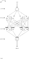
- Fig. 2 shows a schematic diagram of a functional illustration representing a computational graph 200.
- the graph 200 of Fig. 2 corresponds to the neural network 100 shown in Fig. 1 in that it has four layers, with one node per layer for the first and fourth layers, and two nodes per layer for the second and third layers.
- two candidate nodes 21a, 21b are provided as candidates for the first node 21 of the second layer 20.
- two candidate nodes 22a, 22b are provided as candidates for the second node 22 of the second layer 20.
- the same is shown for the third layer 30.
- Two candidate nodes 31a, 31b are provided as candidates for the first node 31 of the third layer 30, and two candidate nodes 32a, 32b are provided as candidates for the second node 32 of the third layer 30.
- the candidate nodes are shown as squares, and the corresponding nodes from Fig. 1 are shown as circles with dashed lines.
- the dashed lines of Fig. 2 show the possible routes along which information may flow through the network, e.g. they show all the possible edges. It is to be appreciated that some of these will be present in each model, and selection of the ones that will be present will depend on the candidate nodes present in said selected model. It is noted that in the example shown in Fig. 2 , each candidate node in the third layer 30 has four possible sources of input from the second layer 20, as does the node 41 in the fourth layer 40.
- a preferred candidate model may be identified.
- the preferred candidate model may be a particular subgraph (e.g. a candidate node may have been selected for each node in the network).
- the particular subgraph may be a combination identified in one of the candidate models, or it may be a new combination of candidate nodes.
- each of the candidate models in a subset of subgraphs included in the computational graph is trained. This process is performed in an iterative fashion. A first candidate model is trained, then, once the first candidate model is trained to a threshold level, a second candidate model is then trained. This is repeated until a selected number of the candidate models have been trained (e.g. all of the candidate models in the subset).
- a controller having a trained policy may analyse the computational graph and the trained models to help identify a candidate model to select for the neural network.
- neural networks here are used for illustration only.
- the computational graph 200 shown in Fig. 2 it would be computationally feasible to train and then test all of the possible combinations of subgraphs, and then select the best-performing one as the model on which the neural network will be based.
- neural networks may be much, much larger than this.
- analysis of a large neural network having a plurality of different options for each node in that network may hold a near-infinite number of possible configurations. To identify a preferred network from this number of configurations, only a subset of the total number of configurations will be used, otherwise the computational requirements would be unpractical.
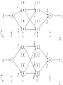
- Figs. 3a and 3b show two schematic diagrams of candidate models for the neural network.
- Fig. 3a shows a candidate model 301 in which nodes 21a, 22b, 31a and 32b have been selected.
- Fig. 3b shows a candidate model 302 in which nodes 21a, 22a, 31a and 32a have been selected. Training of a candidate model is now described with reference to Figs. 3a and 3b .
- the candidate model has a set of candidate nodes selected and a set of weightings ⁇ i,j selected.
- the weightings ⁇ i,j apply a scaling factor to each node-to-node connection in the model.
- the scaling factor for each weighting in the model may be 'learned' by training the model.
- the weightings may be learned, e.g. by using gradient-based learning. This involves defining a cost function and minimising it. Minimising the cost function may be achieved by following the gradient of the cost function in order to minimise it. Stochastic gradient descent may be used as the optimisation procedure. A gradient-descent optimisation algorithm may be used which uses backpropagation. For brevity, these shall not be discussed in much detail.
- ⁇ represents a gradient function, e.g. a derivative.
- a stochastic gradient descent algorithm updates the weightings until conversion.
- Embodiments of the present disclosure place further constraints on the training process.
- a modified loss function is defined which is used during training. When training each model, the updates to the weightings are calculated based on minimising this modified loss function.
- the modified loss function includes a component which takes into account, for a selected weighting, the importance of that weighting in any previously trained models. As different subgraphs may include the same nodes (and their associated weightings), weightings may be trained as part of a later model which have already been trained in relation to an earlier model. This can be seen from Figs. 3a and 3b . These two figures show two possible subgraphs (models) 301,302 from the computational graph 200 shown in Fig. 2 .
- the two subgraphs 301,302 both include nodes 11, 21a, 31a and 41.
- the weightings ⁇ 21 a ,11 , ⁇ 31 a ,21 a and ⁇ 41,31 a are shared by both models (subgraphs 301,302).
- the modified loss function takes into account the importance of that weighting (and its associated node) in an earlier-trained model. For example, this may be based on an indication of the Fisher information for that weighting (and node). Fisher information may provide an indication of the amount of information the node has for the operation of the model. For a selected weighting, the Fisher information provides an indication of the curvature of the log likelihood for that weighting. A Fisher information matrix may be calculated.
- a cross-entropy loss function L m j may be obtained for said subgraph m j .
- the cross-entropy loss function may be defined so that minimising the cross-entropy likelihood provides a maximum likelihood for a classification problem.
- Fisher information for each weighting may be updated sequentially based on the cross-entropy loss function for the subgraph. The update may be based on a derivative of the cross-entropy loss function. For example, a squared gradient of the cross-entropy loss function relative to the selected subgraph may be calculated for each weighting (e.g.
- the update of the Fisher matrix may be calculated using a validation batch after each training of a model, e.g. the updates are determined based on the previously-trained candidate model.
- a loss function L WPL m j may be defined, e.g. for each architecture (subgraph). This will be referred to hereinafter as a weight plasticity loss function.
- This loss function may include a term indicative of Fisher information, e.g. of Fisher information for each weighting.
- the loss function may include a component which, for each weighting, is based on both: (i) a difference between that weighting's value and an optimum value for that weighting, and (ii) an indication of the Fisher information for that weighting, e.g.: ⁇ ⁇ i ⁇ ⁇ m j I ⁇ i ⁇ i ⁇ ⁇ ⁇ i 2
- Minimising the weight plasticity loss function may therefore be based at least in part on minimising this component.
- the optimal weights ⁇ l ⁇ may be overwritten after each training of a model.
- the weight plasticity loss function for each weighting may also include an indication of the cross-entropy loss function for that subgraph.
- the weight plasticity loss function may therefore include the two terms: L m j ⁇ m j + ⁇ ⁇ i ⁇ ⁇ m j I ⁇ i ⁇ i ⁇ ⁇ ⁇ i 2
- Either and/or both of these terms may be scaled, e.g. by a respective hyperparameter.
- Such hyperparameters may be learned. They may be controlled to provide a selected learning rate for the equation.
- the weight plasticity loss function may be minimised. This may have the effect of reducing a magnitude of updates to weightings in a candidate model which are important to other candidate models.
- the weight plasticity loss function balances this minimising of changes to important weightings with a minimising of the performance at performing the image recognition task for each model, so that high performance for the task for each model may still be obtained without sacrificing performance on that same task in earlier trained models.
- the weight plasticity loss function may include a term indicative of a modulus of each weighting. For example, this may be based on a value for the modulus squared, e.g. the weight plasticity loss function may include the term: ⁇ ⁇ i ⁇ ⁇ m j ⁇ ⁇ i ⁇ 2
- Training of each subgraph may be based on minimizing this function when updating the weightings of that subgraph.
- Each of the three components may be scaled according to a hyperparameter to control their relative contributions. Values for these hyperparameters may be learned.
- Updates to the Fisher information matrix may be clipped, e.g. they may be scaled back based on a selected threshold for updates. This may help inhibit exploding gradients associated with the loss function.
- each update may be scaled based on a value for its respective weighting.
- the update to the Fisher information matrix may be scaled based on the norm for each weighting matrix.
- the parameters ⁇ and ⁇ may be tuned, e.g. they can be learned. They may provide a degree of constraint for controlling the learning of the models.
- an analysis of the candidate models is performed.
- the analysis may comprise sequentially evaluating performance of the different candidate models using a validation set, e.g. a data set different to the training data set from which the performance of the model at performing the image recognition task (on unseen data) may be determined.
- the top performing model may be selected.
- the top performing model may be taken as the preferred model, and a neural network may be provided which is based on this preferred model.
- Providing the neural network may comprise creating a neural network using the preferred model and a random set of weightings, then training the network.
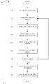
- FIG. 4 Another example is shown in Fig. 4 in which an iterative approach is used which enables a controller to evaluate trained candidate models which have performed well, and to learn from these, and based on this, to suggest candidate models to train and evaluate.
- Fig. 4 shows a method 400 of providing a neural network configured to perform the image recognition task.
- a computational graph is obtained. This may be the same as described above.
- a set of suggested subgraphs is obtained.
- This set of subgraphs may initially be selected randomly. However as the loop iterates, they will be selected by the controller. They may also initially be selected by the controller.
- each of these subgraphs is trained in an iterative fashion, as described above.
- the training uses training data and minimizes a weight plasticity loss function so that updates to weightings of each candidate model are controlled based on how important those weightings are to other previously-trained candidate models.
- each of the candidate models has been trained. They may have been given a limited amount of training time, e.g. only a small number of batches. Each candidate may therefore be better than it was before, but not fully trained.
- a time threshold or batch threshold may be used to control the amount of training each model receives. They are then tested on a validation data set so that a best candidate model can be identified. The best candidate model is then evaluated by a controller.
- the controller may use reinforcement or evolutionary learning algorithms to update parameters of its policy based on results from the validation data for the best candidate model. For example, the controller may use a reinforcement learning algorithm.
- Reinforcement learning uses a trial and error process guided by an agent.
- the agent may interact with its environment in discrete or continuous time.
- the choice of this action is done by the policy ⁇ ⁇ p ( a
- the agent receives a new state S t +1 and a reward R t +1 .
- the objective maximizes some form of future reward.
- Reinforcement learning comprises changing the policy in response to a received reward and aiming to maximize a future reward. In order to do so, the reinforcement learning algorithm may address an exploration-exploitation trade off.
- bandit algorithms may be used.
- this may comprise identifying new, untested combinations/selections of nodes which have unknown performance capabilities, and sticking to known combinations/selections of nodes whilst making small changes to the combination/selection.
- Parameters for the policy of the controller may be learned using policy gradient methods, e.g. methods based on a gradient of a loss function.
- Policy gradient methods may be used in combination with a recurrent policy adapted to neural architecture search.
- An architecture e.g. a subgraph
- Each action may define an operation (e.g. the functionality of a node), such as a ReLU or softmax function.
- Each action may define an indication of how to compose an operation (e.g. defining the input of operations).
- the policy e.g. a recurrent neural network policy
- the state S T may be considered the hidden state of the neural network.
- the policy may be defined as: ⁇ ⁇ p a t
- s t ⁇ ⁇ p a t
- a 1 , ... , t ⁇ 1 P ⁇ p a t
- D defines the set of all possible architectures (subgraphs)
- ⁇ ⁇ p ( a 1 , ..., T ) is the probability of sampling the architecture a 1 , ..., T
- R (a 1 , ..., T ) is the inverse of the validation perplexity of the sampled architecture a 1 , ..., T.
- the gradient may be computed using a Monte Carlo estimate, e.g. which is unbiased.
- REINFORCE may be used.
- a Boltzmann softmax equation may be used which divides exponentials in the original softmax by a temperature T which decays over time. This temperature (and its decay) may be used to initially favour exploration (e.g. as opposed to exploitation).
- a validation set (different to the training data set used for updating the weightings) may be used. This may enable the policy to select models that generalize well (rather than ones which are too specialized/overfitted to the training data set). For example, the perplexity may be calculated on a validation data set (or a minibatch thereof).
- the controller's policy may be updated. This may be based on the approach described above.
- the updated policy may then select different subgraphs/identify different subgraphs it considers to be better.
- the controller may be configured to suggest further subgraphs which may be considered by the controller to be, as determined based on its updated policy, suitable for performing the image recognition task.
- the controller may be operated to use the updated policy to suggest subgraphs for the image recognition task. For example, it may select a set of actions corresponding to a sequence of operations for the subgraph. A plurality of such subgraphs may be selected by the controller. These may then form the candidate models for the next round of testing subgraphs.
- the controller may not suggest subgraphs. Steps 420 to 470 may be looped without suggesting new subgraphs so that the candidate models obtained at step 420 are trained for several iterations. During each iteration of training these candidate models, the policy may still be updated based on the evaluation of the trained models. In some examples, the controller may not suggest subgraphs, but may still provide an indication of which of a selection of trained subgraphs is the preferred subgraph. For example, step 460 may be skipped.
- step 470 it may be determined whether or not to iterate (e.g. repeat steps 420 to 460).
- the subgraphs suggested by the controller may be examined to determine this. Different criteria may be used in this step to determine whether or not to keep iterating.
- the suggested subgraphs may be used in step 420 as the obtained set of subgraphs, and steps 420 to 460 may be repeated using these newly-suggested candidate models. By iterating this process, the method may get closer to obtaining a preferred model for performing the image recognition task.
- Criteria may be applied to determine whether a suggested subgraph, or the best subgraph from the previous set of candidate models, should be used as the preferred model which the neural network will use for performing the image recognition task. For example, a comparison may be made between a suggested candidate model and the previous best candidate model. If the two are functionally very similar, e.g. have an architectural degree of similarity above a threshold level/contain a threshold number of the same neurons (e.g. in the same location in the network), it may be determined that the suggested model/the previous best model should be taken as the preferred model. If the controller suggests a plurality of different subgraphs, a comparison may be performed to see if any of these have been previously suggested by the controller.
- a threshold number of suggested subgraphs are the same as previous candidate models, then it may be determined that no meaningful changes have occurred, and the threshold may be determined to have been reached. Additionally and/or alternatively, a threshold time limit, or threshold number of iterations may be applied, and once this threshold is reached, the method may stop iterating.
- step 470 If at step 470, it is determined that iteration should stop, the method proceeds to step 480.
- step 480 a neural network is created based on the subgraph in the preferred model.
- this neural network is trained so that the weightings are updated to convergence, e.g. starting from a random initialization. This network is then provided as the selected neural network for performing the image recognition task.
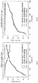
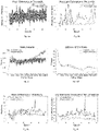
- Figs. 5a and 5b show results for test accuracy when sequentially training two models.
- the two models were tested on the hand digit recognition dataset (MNIST).
- the two models were simple feedforward networks, with model 1 having 4 layers and model 2 having 6 layers. In both cases, the first model was trained until convergence, thus obtaining ( ⁇ 1 , ⁇ s ), which are the optimum weightings for model 1.
- the optimum weightings for model 1 include some weightings which are shared with model 2.
- Model 2 is then trained on the same data set as model 1. Training model 2 includes updating the shared weightings.
- Figs. 5a and 5b show how the test accuracy for these two models varies depending on the loss function used when training the models.
- Fig. 5a shows results when sequentially training two models using a cross-entropy loss function, e.g. it is trained by maximum likelihood of obtaining optimum weightings.
- the green line (which goes from top left to top right) shows the performance of model 1 after training. This is a flat line, which shows the performance achieved by model 1 remains at a test accuracy of approximately 92%. This line shows the performance of model 1 as a baseline.
- the blue line (which goes from bottom left to top right) shows the test accuracy of model 2 whilst this model is being trained. As expected, the test accuracy of model 2 increases with increased training. It can be seen that model 2 does not quite reach convergence over the number of iterations shown, but that a substantial increase in the ability of model 2 to perform the task has been observed.
- Fig. 5a The red line in Fig. 5a (top left to middle right) shows how the test accuracy of model 1 is affected by the training of model 2 (and thus updating of weightings shared between the two models). As can be seen, as model 2 is trained (and the shared weightings are changed) the performance of model 1 decreases. It is apparent from Fig. 5a that the drop in performance of model 1 is substantial, and so any subsequent analysis of model 1 would suggest that model 1 does not perform as well as it is capable of performing. As can be seen, over 500 iterations in training, the test accuracy of model 1 dropped almost 30%.
- Fig. 5b shows results when sequentially training two models using a weight plasticity loss function:
- L WPL m j ⁇ 2 ⁇ s L 2 ⁇ 2 ⁇ s + ⁇ 2 ⁇ ⁇ s i ⁇ ⁇ s I ⁇ s i ⁇ s i ⁇ ⁇ ⁇ s i 2 + ⁇ 2 ⁇ ⁇ s 2 i ⁇ ⁇ s , ⁇ 2 ⁇ ⁇ s 2 i ⁇ 2
- the lines represent the same indicators as in Fig. 5a .
- the performance of model 1 after training and the performance of model 2 during training are roughly the same as in Fig. 5a .
- the main difference is the test accuracy for model 1 whilst training model 2.
- the second optimization e.g. the training of model 2 predominantly modifies weightings that have low Fisher information. These are considered to be less important for the first model (e.g. because the Fisher information indicates the curvature of the log likelihood with regard to each particular weighting).
- Training model 2 using a loss function based on how important to model 1 the nodes and/or edges associated with a weighting are enables performance of model 1 to be retained during training of a subsequent model.
- Figs. 5a and 5b it can be seen that an analysis of model 1 and model 2 at iteration 500 of training model 2 would provide a different indication of which the model with the higher test accuracy.
- By training using the weight-plasticity loss function test accuracy of model 1 is preserved whilst training model 2.
- Figs. 6a to 6f show further comparative data between use of a weight-plasticity loss function and a cross-entropy loss function.
- I ⁇ i t + 1 ⁇ I ⁇ i t + ⁇ L m j ⁇ ⁇ i ⁇ ⁇ m j 2 , ⁇ i ⁇ ⁇ m j , I ⁇ i t , otherwise .
- I w t + 1 ⁇ ⁇ I w t , ⁇ I w t ⁇ ⁇ ⁇ , ⁇ I w t ⁇ I w t ⁇ , otherwise .
- values for ⁇ and ⁇ were set to 1 and a 100 respectively, with 50 models being sampled per epoch, with 10 batches per epoch.
- the weight-plasticity loss function was introduced at the third epoch, and the Fisher information was set to zero at each epoch.
- the cross-entropy loss function a cross-entropy loss function was used throughout. Increasing the value of ⁇ places a larger constraint (e.g. penalty) on previously learned weightings.
- Fig. 6a shows mean difference in perplexity, for each trained model, between performances of: (i) that model after the sequential training of all of the 50 models, and (ii) that model when trained independently. This difference is shown over 50 epochs.
- Perplexity provides an indication of how well a model predicts a sample - a low perplexity indicates that the model predicts well.
- Fig. 6a also shows error bars for ⁇ 2 standard deviations.
- the use of weight-plasticity loss function (as shown by the lower of the two lines at the right-hand end, and the narrower of the two error bars) reduces the mean difference in perplexity between a model that has been sequentially trained and a model that has been independently trained. This is clearly beneficial. It means that models used for updating a policy of the controller are more reliably the correct choice (e.g. the selection of a best candidate model is less likely to have been skewed by the location in the sequence at which that model was trained).
- Fig. 6b shows the maximum difference in perplexity between performances of: (i) models after the sequential training of all of the 50 models, and (ii) corresponding models when trained independently.
- the weight-plasticity loss function provides a substantial reduction in the maximum difference in perplexity. Also, the fluctuations in this value are lower for the weight-plasticity loss function. This shows another clear benefit of using the weight-plasticity loss function.
- Figs. 6c to 6f show values for ⁇ and ⁇ were set to 70 and 10 respectively, with 70 models per epoch, with each model being trained for 15 batches.
- updates to the weightings are based on the weight-plasticity loss function at the eighth epoch, with the Fisher information matrix set to zero at each three epochs.
- 2000 steps per epoch are used to train the policy and the policy is not held fixed.
- Reinforcement learning algorithm REINFORCE was used as part of the controller with a policy to be determined.
- Fig. 6c shows the mean reward for the models plotted against the number of policy steps taken.
- the policy is designed to maximize the reward based on the candidate models, so a higher value for the reward is beneficial.
- the mean reward when using the weight-plasticity loss function is substantially higher than when using the cross-entropy loss function.
- the error bars shown represent 0.5 standard deviations. It can be seen that the mean reward is much higher for the weight-plasticity loss function and the standard deviation of this reward is much lower.
- Fig. 6d shows the entropy for the policy.
- the entropy of a policy provides a measure of the uncertainty of the probability distribution of the predictions made by the policy - the higher the entropy, the higher the uncertainty.
- the entropy of the policy obtained using the weight-plasticity loss function is substantially less than that obtained using the cross-entropy loss function.
- use of the weight-plasticity loss function may provide a more reliable neural network for performing an image recognition task.
- Figs. 6e and 6f show similar trends to graphs 6a and 6b in that when comparing models trained as part of a sequence using the weight-plasticity loss function to corresponding models trained independently, the mean and standard deviation of this difference over a number of candidate models is substantially lower than when using a cross-entropy loss function. Additionally, it is very apparent from Figs. 6e and 6f that the use of the weight-entropy loss function is responsible for this increase in performance. As mentioned above, the weight-plasticity loss function was only introduced at the eighth epoch. Before this point, the two loss functions were identical. As can be seen from Figs. 6e and 6f , the improvement in performance of the weight-plasticity loss function occurs after the eighth epoch. Prior to this, the two loss functions perform the same.
- the disclosure herein has made reference to nodes of the neural network.
- the functionality e.g. activation functions used in a neural network are generally known. Such functions may include: ReLU, Tanh, Sigmoid, Softmax etc. In particular, non-linear functions are used frequently. These functions may be used for individual neurons in a network.
- Embodiments of the present disclosure encompass each individual node (as described herein) being either an individual neuron or a block of neurons.
- the computational graph may include combinations of both.
- Embodiments of the present disclosure may utilize blocks of neurons at nodes.
- Each block of neurons may its own set topography and contents.
- a block may include a sequence of selected neurons connected by a selected set of edges, with fixed weightings associated therewith.
- Use of blocks of neurons may improve the neural architecture search as blocks may be selected based on previous knowledge of how those blocks perform on similar tasks. This may also reduce the number of weightings which need to be trained as part of the method because the weightings within a block may be held fixed.
- the neural architecture search methods may only then need to identify the edges and weightings between different blocks, e.g. between fewer features than if the blocks were expanded out and edges/weightings were needed for every neuron.
- Such examples may be referred to as neural architecture search with blocks.
- a controller may be used (e.g. with a LTSM policy) which samples blocks at nodes and determine edges at which to connect them.
- the internal weightings for a block may not be held fixed, e.g. instead only the component neurons are selected, but the weightings between them may be edited during training.
- weight plasticity loss functions may find particular application in such scenarios.
- a reward to be maximized by the controller may be modified to include a component which takes into account complexity of a candidate model.
- the reward may be based on the number of components within a candidate model. This may be in addition to the reward being based on a goodness of fit for a candidate model, e.g. a validation perplexity for the model. It is to be appreciated that introducing a component based on complexity of a candidate model into the reward function may be applicable to all methods described herein.
- a density based reward may be introduced.
- the reward may be configured to favour models with fewer weightings.
- ⁇ maximum is the maximum possible number of weightings to be included in the model.
- ppl is the validation perplexity, e.g. how well a model performs on a validation data set.
- the two components of the reward may be separated (as shown) to prevent the reward from turning negative. Use of this reward may therefore identify models which perform well and which have fewer weightings.
- Examples described herein have included use of iterative processes where candidate models are trained numerous times before a preferred model is selected.
- the same set of candidate models may be trained a number of times, e.g. they may be trained on a number of different batches.
- the iterative process may include multiple repetitions of training a set of candidate models and then evaluating the same models using the controller to update the policy, before re-training the same models and then re-evaluating them with the controller.
- the controller may suggest new candidate models for testing in response to having updated the policy based on a set of trained candidate models.
- the iterative process may not be needed.
- a single operation of sequentially training of candidate models may be enough for a preferred model to be identified.
- embodiments described herein enable sequentially trained models to be trained so that any updated weightings reduce the detriment to earlier-trained models, one run of sequentially training these models may still be enough for a preferred model to be identified.
- Obtaining a computational graph may be considered to be obtaining data indicative of a computational graph, such as an array of matrices and operations for controlling and scaling the flow of information between different functions.
- One particular subgraph e.g. collection of nodes, connected by edges with weightings included
- the candidate model is determined to be a preferred candidate model
- the particular architecture of the subgraph may be used as the architecture for the neural network (e.g. without the presence of the other nodes and edges in the computational graph). is to be appreciated that the present disclosure is not linked to the provision of any particular type of neural network.
- suitable neural networks may include convolutional neural networks, deep residual neural networks, capsule networks, recurrent neural networks, multi-layer perceptrons etc.
- Neural networks disclosed herein may include recurrent neural networks used for encoders in sequence to sequence models which are of particular importance. These may find application in e.g. translation, churn detection and email classification.
- improved translation neural networks may be able to identify key phrases in a sentence which are to be translated. This may enable neural networks which can receive input data in the form of a string of text in a first language or coding, process this input data to provide output data in the form of a string of text in a different language or coding.
- neural networks may find application in image recognition systems. For example, at security checkpoints e.g. airports, a camera may capture an image of an individual, and the neural network may be arranged to classify/identify the individual. Improved neural network architectures may improve the ability of these neural networks to identify individuals in photos.
- controller/policy may be used during the analysis of trained candidate models. Whilst use of reinforcement learning has been described, other examples could be used. For example, evolutionary networks (and associated neuroevolutionary methods) may be used. In such examples, both the topology of the network and its weightings may be updated during training (e.g. the network architecture may evolve). Weightings may also be inherited by child nodes in a controlled manner, so that parental weightings may be applied to a child node where suitable.
- each node may comprise a signal processing unit configured to receive an input signal, process the input signal and provide an output signal.
- Nodes may comprise circuitry configured to: receive at least one input signal indicative of an item of input data from a preceding node connected to said node via an edge, perform an operation on the input data to provide output data, optionally scale the input data according to a weighting associated with said node; and provide an output signal indicative of the output data to a subsequent node via an edge in the graph.
- Edges may comprise communication paths configured for the transmission of signals between nodes.
- the communication paths may be configured to receive an output signal from a preceding node, optionally scale that output signal according to a weighting, and transmit that output signal to a subsequent node.
- Localised data storage may be used for determining an end destination for transmitting the output signal to via the communication path.
- Computer programs include software, middleware, firmware, and any combination thereof. Such programs may be provided as signals or network messages and may be recorded on computer readable media such as tangible computer readable media which may store the computer programs in non-transitory form. Methods described herein and/or the functionality of components such as nodes and edges may be provided in hardware which includes computers, handheld devices, programmable processors, general purpose processors, application specific integrated circuits (ASICs), field programmable gate arrays (FPGAs), and arrays of logic gates.
- ASICs application specific integrated circuits
- FPGAs field programmable gate arrays
- one or more memory elements can store data and/or program instructions used to implement the operations described herein.
- Embodiments of the disclosure provide tangible, non-transitory storage media comprising program instructions operable to program a processor to perform any one or more of the methods described and/or claimed herein and/or to provide data processing apparatus as described and/or claimed herein.
- H p ( ⁇ 1 , ⁇ s ) H ( ⁇ 1 , ⁇ s ) + ⁇ -2 I p be the negative Hessian of l p ( ⁇ 1 , ⁇ s ).
- l p ⁇ 1 ⁇ s l p ⁇ ⁇ 1 ⁇ ⁇ s ⁇ 1 2 ⁇ 1 ⁇ s ⁇ ⁇ ⁇ 1 ⁇ ⁇ s T H p ⁇ ⁇ 1 ⁇ ⁇ s ⁇ 1 ⁇ s ⁇ ⁇ ⁇ 1 ⁇ s ; the first derivative is zero since it is evaluated at the maximum likelihood estimate.
- Equation (4.5) depends only on the log likelihood of the second model f ( ; ⁇ 2 , ⁇ s ).
- the information learned from the first model f ( ; ⁇ 1 , ⁇ s ) is contained in the conditional posterior probability log p ( ⁇ 1 , ⁇ s
- the last term in the right hand side of Equation (4.5), 1 2 ⁇ T ⁇ ⁇ must hold the interaction between the models f ( ; ⁇ 2 , ⁇ s ) and f ( ; ⁇ 1 , ⁇ s ).
- ) is intractable. We approximate it as a Gaussian distribution centered at the maximum likelihood estimate ( ⁇ 1 , ⁇ s ) and with variance the diagonal of the observed Fisher information.
- H ( ⁇ 1 , ⁇ s ) I( ⁇ 1 , ⁇ s ).
- Equation (4.5) i.e., log p ( ⁇ 2 , ⁇ s ), will stand for an l 2 regularization.
Landscapes
- Engineering & Computer Science (AREA)
- Theoretical Computer Science (AREA)
- Physics & Mathematics (AREA)
- Life Sciences & Earth Sciences (AREA)
- Health & Medical Sciences (AREA)
- Artificial Intelligence (AREA)
- General Physics & Mathematics (AREA)
- Data Mining & Analysis (AREA)
- General Engineering & Computer Science (AREA)
- Computational Linguistics (AREA)
- Evolutionary Computation (AREA)
- General Health & Medical Sciences (AREA)
- Software Systems (AREA)
- Computing Systems (AREA)
- Biophysics (AREA)
- Mathematical Physics (AREA)
- Molecular Biology (AREA)
- Biomedical Technology (AREA)
- Bioinformatics & Cheminformatics (AREA)
- Bioinformatics & Computational Biology (AREA)
- Evolutionary Biology (AREA)
- Physiology (AREA)
- Audiology, Speech & Language Pathology (AREA)
- Computer Vision & Pattern Recognition (AREA)
- Image Analysis (AREA)
Description
- The present disclosure relates to the field of neural architecture search. In particular, the present disclosure relates to systems and methods for designing neural networks.
- Through the provision of increased computing power and access to increasingly large quantities of suitable training data, machine learning techniques have found increasing application for providing improved solutions to many technical problems. In particular, use of neural networks has become increasingly common as a way of providing neat and effective solutions to many such technical problems.
- Neural networks typically have a structure which includes a plurality of interconnected neurons. Each neuron in the network is arranged to receive input data, which it scales and performs a function on before providing some output data. This output data may then be fed into subsequent neurons as their input data. These subsequent neurons may then also scale this data before performing further functions on it. This process may be repeated for many different neurons before a final output is decided. These networks may be trained by using input data which has a known output corresponding to it, where training involves repeatedly operating the network on the data to provide an output and performing a comparison with this output. That is, the output for a piece of input data is compared to the known output corresponding to that piece of input data. Weights of the network (which effect the scaling of input data) may then be updated based on the results of this comparison so that the network 'learns' to provide the correct output when provided with a given piece of input data. By repeating this process many times with suitable training data, it has been shown that neural networks can develop great ability to be universal approximators (e.g. they can address the problems they are trained for).
- Numerous different structures for neural networks exist. For example, feedforward neural networks comprise a plurality of layers of neurons. In feedforward networks, the output of a neuron in one layer is fed into every neuron in the subsequent layer, so that each neuron receives an input from neurons in their preceding layer. Different configurations of neural networks include recurrent neural networks in which the input for a preceding layer may also be fed into the subsequent layer as input data. Another type of network is a residual network which has a similar arrangement to a simple feedforward network, except that the network may include branches which connect the output from neurons, or layers of neurons, to neurons in layers other than the subsequent layer. Different types of network have been found particularly effective at solving certain types of technical problems. Therefore, when designing a neural network, it can be beneficial to select a type of network based on the problem that network aims to address.
- Whilst the selection of the type of neural network can have a significant bearing on the overall ability of the network to perform a selected task, the selection of the type of constituent neurons can also have a significant impact on the ability of a network to perform a selected task. For example, a well-trained network made up of a first selection of neurons may have inferior performance to a less well-trained network with a different, better, selection of neurons. As the training of a network can be very time-consuming, initially selecting suitable neurons can provide a significant reduction in the time, and resources, taken to provide a neural network which performs satisfactorily for a selected task. In addition to increasing the efficiency of training a neural network, the ability to select a suitable configuration of neurons may make the difference between the provision of a neural network which can solve a technical problem, and one which cannot.
- Embodiments of the present disclosure may address these and other technical problems through the provision of systems and methods of neural architecture search to provide a neural network configured to solve, or contribute towards a solution to, a selected technical problem.
- Hieu Pham et al. 'Efficient Neural Architecture Search via Parameter Sharing', 09 February 2019, discloses a method for neural architecture search.
- James Kirkpatrick et al. 'Overcoming catastrophic forgetting in neural networks', 28 March 2017, discloses an algorithm for elastic weight consolidation.
- The invention is set out in the appended independent claims. Preferred embodiments are defined in the appended dependent claims. Independent claim 1 is directed to a computer-implemented method and independent claim 13 is directed to a computer program product.
- Some embodiments will now be described, by way of example only, with reference to the figures, in which:
-
Fig. 1 shows a schematic diagram of an example feed forward network. -
Fig. 2 shows a schematic diagram of an example graph including a feed forward network having two possible node options at each node in the second and third layers. -
Fig. 3a shows a schematic diagram of one example feed forward network selection from the options available as shown inFig. 2 . -
Fig. 3b shows a schematic diagram of another example feed forward network selection from the options available as shown inFig. 2 . -
Fig. 4 shows a flow chart for an example method of neural architecture search. -
Figs. 5a and 5b show a comparison between results obtained using a conventional cross-entropy loss system and using a weight-plasticity loss system of the present disclosure. -
Figs. 6a to 6f show a comparison between results obtained using a conventional cross-entropy loss system and using a weight-plasticity loss system of the present disclosure. - In the drawings like reference numerals are used to indicate like elements.
- Embodiments of the present disclosure relate to computer-implemented methods of neural architecture search. When faced with the job of having to provide a neural network configured to perform an image recognition task, the neural architecture search is used to identify a preferred model for such a neural network. A preferred model is identified based on an analysis of multiple candidate models. Identifying a preferred model involves providing a computational graph made up of a plurality of different nodes which are connected by a plurality of edges. The computational graph is considered to provide a plurality of subgraphs (which are considered to be 'candidate models'). Each subgraph is a selection of some of the nodes and edges from the computational graph.
- The computational graph includes a plurality of weightings which scale information as it flows through the network (e.g. between different nodes). Between nodes, a weighting is applied so that items of input data received at a node are scaled based on the preceding node from which they have been received. A plurality of different subgraphs is identified, and any two of these different subgraphs both include some of the same nodes and weightings. The identified subgraphs represent a subset of all the possible configurations of nodes and edges from the computational graph.
- The identified subgraphs are trained sequentially using training data associated with the image recognition task. Training of a subgraph includes repeatedly operating the subgraph on items of training data which have a known output associated therewith. For each item of training data, the output from operating the subgraph on that input data is compared to the known output associated with that item of training data. By comparing the two outputs, the weightings of the subgraph may be modified based on a difference between the two outputs (e.g. so that if the network were to operate on that input data again, it would provide an output corresponding to the known output). This process is repeated a number of times before the subgraph is determined to be 'trained', e.g. once there has been a convergence on its ability to perform the image recognition task.
- Once a first subgraph is trained, a second subgraph is then trained in much the same way. However, embodiments of the present disclosure place constraints on how the weightings of the second subgraph may be updated. The first and second subgraphs may have an overlap in their selection of nodes and edges (and thus associated weightings). The weightings that also featured in the first subgraph (hereinafter referred to as 'shared weightings') will have already had their values updated and refined based on training the first subgraph to perform the image recognition task. When updating the weightings associated with nodes in the second subgraph in response to training, updates to each shared weighting are controlled based on an indication of how important to the first subgraph that shared weighting is.
- A plurality of different subgraphs is trained sequentially. Based on an analysis of the trained subgraphs, a preferred model for the neural network is identified. In some examples, a controller (e.g. a reinforcement learning controller) may be used to evaluate trained subgraphs and to suggest further subgraphs for sampling based on the results of the evaluation of the trained subgraphs. This process may be iterated until a preferred model has been identified. The preferred model may be any subgraph, e.g. any combination of the nodes and edges (and associated weightings) from the computational graph. A neural network configured to perform the image recognition task is provided based on the preferred model. By controlling updates to weightings which are important for at least one of the earlier-trained identified subgraphs based on an indication of how important they are to the earlier-trained subgraph, embodiments may provide less of a time-dependent bias to the neural architecture search. For example, weightings associated with nodes and edges which were important to an earlier-trained subgraph may not have their associated weightings changed as much in response to subsequent training of a different subgraph. Models which made use of such nodes and edges may be very suitable for providing a neural network configured to perform the image recognition task. By controlling the updates to weightings associated with such nodes and edges indicated to be important, the earlier-trained models may no longer lose an ability to perform the task as well, despite subsequent models being trained (and thus changes being made to some nodes in the earlier-trained model). As a consequence, subsequent analysis of the trained candidate models may be less biased towards the later-trained models. Instead, this may enable earlier-trained models to still be looked upon favourably, if relevant, and so they, e.g. weights that they used and that are shared with the candidate that will be the final one, may feature in a final architecture for the neural network, whereas previously they may have been overlooked as a consequence of important weightings being changed. The results of the neural architecture search may therefore provide an improved neural network for performing the image recognition task.
- Embodiments of the present disclosure will now be described with reference to the Figures.
Fig. 1 shows a schematic of a very simple feedforwardneural network 100. It is to be appreciated that the present disclosure is applicable to all forms of neural network, and that thenetwork 100 ofFig. 1 is just used as a simple schematic to illustrate the teaching of the present disclosure. - The feedforward
neural network 100 ofFig. 1 has four layers: afirst layer 10, asecond layer 20, athird layer 30 and afourth layer 40. Thefirst layer 10 includes onenode 11. Thesecond layer 20 includes twonodes third layer 30 which hasnodes fourth layer 40 has asingle node 41. Edges which connect different nodes are shown by arrows inFig. 1 . For example, as can be seen, an edge connectsnode 11 tonode 21, and another edge connectsnode 11 tonode 22. Thenetwork 100 includes a plurality of weightings θ i,j , where each θi,j represents a scaling factor applied to the input to node i which has been received from the output of node j. At each node a scaling factor is applied to each edge arriving at that node. It is to be appreciated that the weightings may be applied at each edge or at each node. Weightings will hereinafter be referred to as being associated with a node, but this is not to be considered limiting. Rather, the weighting associated with a node means that said node will process input data which has been scaled according to that weighting. - The
node 11 in thefirst layer 10 is configured to receive an input. The input may be some form of data which is to be processed by theneural network 100. Processing this data may enable theneural network 100 to provide an output. The output may be based on an analysis of this data, as performed by theneural network 100. The output may provide an indication of the contents of the input data. For example, the input data may comprise a photo, and the output provides an indication of what is shown in the photo. - The
node 11 in thefirst layer 10 is configured to process the received input data based on a certain functionality specified at thisnode 11. Thenode 11 in thefirst layer 10 is arranged to then provide this processed data to each of the twonodes second layer 20. Each of the twonodes second layer 20 are configured to then process this data received from thefirst layer 10 based on certain functionality specified for thatnode node 11 in thefirst layer 10. - Each of the
nodes second layer 20 is configured to then output their processed data and provide it to each of thenodes third layer 30. Again, each of the twonodes third layer 30 are configured to then process this data received from thesecond layer 20 based on certain functionality specified for that node and a scaling factor applied to this processed data. As can be seen inFig. 1 , each of thenodes third layer 30 receives input data from two precedingnodes 21,22 (the nodes in the second layer 20), as opposed to receiving input data from one node. Each of thenodes third layer 30 is configured to process their input data and provide their processed output data to thenode 41 in thefourth layer 40. Thenode 41 in thefourth layer 40 is configured to then provide an output value based on processing this data received from thethird layer 30 based on certain functionality specified for thatnode 41 and a scaling factor applied to this processed data. - It is to be appreciated that the skilled person would be aware of examples of the type of functionality provided by each node in the
network 100. There are numerous factors which contribute to the ability of a neural network to perform its image recognition task. For example, the size and/or depth of a network (e.g. the number of nodes/the number of layers of nodes) will influence the performance of a neural network. With regard toFig. 1 , it is to be appreciated that the performance of thisnetwork 100 will, amongst other factors, depend on the weightings θi,j and the functionality applied at each of the nodes in thenetwork 100. Embodiments of the present disclosure may enable an improved selection of the nodes for the network, and thus may enable the provision of an improved neural network for performing the image recognition task. - When determining which nodes to select for the
network 100, a computational graph is constructed. The computational graph includes a plurality of nodes connected by a plurality of edges. Each node is configured to receive at least one item of input data from a preceding node connected to it via an edge. Each node is arranged to process input data by applying a weighting to the input data and performing an operation on the weighted input data to provide output data. Different nodes may perform different operations, e.g. they may have different functionalities. The graph includes a weighting associated with each node for scaling that node's input data. Each node is configured to provide its output data to a subsequent node via an edge in the graph. The computational graph is considered to define a plurality of candidate models, each candidate model being a subgraph in the computational graph. Each subgraph is made up of a selection from the computational graph of the plurality of nodes and edges, and the weightings associated with said selected nodes. Some of the nodes and their associated weightings are shared between both different subgraphs. - Each candidate model may comprise a fixed, selected arrangement of nodes. The selected architecture (e.g. arrangement of nodes) may vary between different candidate models. The functionality provided at each node may vary between different candidate models. At each of these nodes, a plurality of options for the functionality of that node may be provided. The options for each node may be considered to be represented as a series of candidate nodes clustered together at a selected location in the graph (e.g. in a region where the selected node would be in the final neural network). The computational graph may include weightings for connections between each candidate node in a cluster to each candidate node in a subsequent cluster.
-
Fig. 2 shows a schematic diagram of a functional illustration representing acomputational graph 200. Thegraph 200 ofFig. 2 corresponds to theneural network 100 shown inFig. 1 in that it has four layers, with one node per layer for the first and fourth layers, and two nodes per layer for the second and third layers. - In the
graph 200 ofFig. 2 , twocandidate nodes first node 21 of thesecond layer 20. Likewise, twocandidate nodes second node 22 of thesecond layer 20. The same is shown for thethird layer 30. Twocandidate nodes first node 31 of thethird layer 30, and twocandidate nodes second node 32 of thethird layer 30. The candidate nodes are shown as squares, and the corresponding nodes fromFig. 1 are shown as circles with dashed lines. - The dashed lines of
Fig. 2 show the possible routes along which information may flow through the network, e.g. they show all the possible edges. It is to be appreciated that some of these will be present in each model, and selection of the ones that will be present will depend on the candidate nodes present in said selected model. It is noted that in the example shown inFig. 2 , each candidate node in thethird layer 30 has four possible sources of input from thesecond layer 20, as does thenode 41 in thefourth layer 40. Once acomputational graph 200 has been created with candidate models (subgraphs) included, a preferred candidate model may be identified. The preferred candidate model may be a particular subgraph (e.g. a candidate node may have been selected for each node in the network). The particular subgraph may be a combination identified in one of the candidate models, or it may be a new combination of candidate nodes. - To identify the preferred candidate model, each of the candidate models in a subset of subgraphs included in the computational graph is trained. This process is performed in an iterative fashion. A first candidate model is trained, then, once the first candidate model is trained to a threshold level, a second candidate model is then trained. This is repeated until a selected number of the candidate models have been trained (e.g. all of the candidate models in the subset). As discussed in more detail below, once the candidate models have been trained, a controller having a trained policy may analyse the computational graph and the trained models to help identify a candidate model to select for the neural network.
- It is to be appreciated that the schematic diagrams of neural networks here are used for illustration only. For the
computational graph 200 shown inFig. 2 , it would be computationally feasible to train and then test all of the possible combinations of subgraphs, and then select the best-performing one as the model on which the neural network will be based. However, neural networks may be much, much larger than this. As such, analysis of a large neural network having a plurality of different options for each node in that network may hold a near-infinite number of possible configurations. To identify a preferred network from this number of configurations, only a subset of the total number of configurations will be used, otherwise the computational requirements would be unpractical. -
Figs. 3a and 3b show two schematic diagrams of candidate models for the neural network.Fig. 3a shows acandidate model 301 in whichnodes Fig. 3b shows acandidate model 302 in whichnodes Figs. 3a and 3b . - The candidate model has a set of candidate nodes selected and a set of weightings θi,j selected. The weightings θi,j apply a scaling factor to each node-to-node connection in the model. The scaling factor for each weighting in the model may be 'learned' by training the model.
- The weightings may be learned, e.g. by using gradient-based learning. This involves defining a cost function and minimising it. Minimising the cost function may be achieved by following the gradient of the cost function in order to minimise it. Stochastic gradient descent may be used as the optimisation procedure. A gradient-descent optimisation algorithm may be used which uses backpropagation. For brevity, these shall not be discussed in much detail.
- Each weighting θi,j may be trained according to:

- Given a family of density models (pmodel;θ), conventional neural networks may be trained using a maximum likelihood (e.g. a maximum likelihood function). For example, it is to be appreciated that these density models represent probability density functions for the models given a particular set of weightings. That is, they are trained to identify so-called 'optimum weightings' θ̂ for the network based on e.g.

- By assuming that xi iidUniform(x 1, ... xn ), and by Bayes' theorem, it can be taken that:

- A maximum likelihood estimator may identify the 'optimum weightings' by minimizing:

- Embodiments of the present disclosure place further constraints on the training process. A modified loss function is defined which is used during training. When training each model, the updates to the weightings are calculated based on minimising this modified loss function. The modified loss function includes a component which takes into account, for a selected weighting, the importance of that weighting in any previously trained models. As different subgraphs may include the same nodes (and their associated weightings), weightings may be trained as part of a later model which have already been trained in relation to an earlier model. This can be seen from
Figs. 3a and 3b . These two figures show two possible subgraphs (models) 301,302 from thecomputational graph 200 shown inFig. 2 . As can be seen, the two subgraphs 301,302 both includenodes - When updating a weighting in a candidate model, the modified loss function takes into account the importance of that weighting (and its associated node) in an earlier-trained model. For example, this may be based on an indication of the Fisher information for that weighting (and node). Fisher information may provide an indication of the amount of information the node has for the operation of the model. For a selected weighting, the Fisher information provides an indication of the curvature of the log likelihood for that weighting. A Fisher information matrix may be calculated.
- For example, for a selected subgraph (model) to be trained, a cross-entropy loss function


j ). This may then be used to update the Fisher information for each weighting, e.g. The Fisher information for each weighting (Iθi ) may be updated sequentially on j ∈ {1, ..., n} as:
- For all i ∈ {1, ..., |θ|}. The update of the Fisher matrix may be calculated using a validation batch after each training of a model, e.g. the updates are determined based on the previously-trained candidate model.
- A loss function


- Minimising the weight plasticity loss function may therefore be based at least in part on minimising this component. The optimal weights

- The weight plasticity loss function for each weighting may also include an indication of the cross-entropy loss function for that subgraph. The weight plasticity loss function may therefore include the two terms:

- Either and/or both of these terms may be scaled, e.g. by a respective hyperparameter. Such hyperparameters may be learned. They may be controlled to provide a selected learning rate for the equation.
- When training each of the candidate models, the weight plasticity loss function may be minimised. This may have the effect of reducing a magnitude of updates to weightings in a candidate model which are important to other candidate models. The weight plasticity loss function balances this minimising of changes to important weightings with a minimising of the performance at performing the image recognition task for each model, so that high performance for the task for each model may still be obtained without sacrificing performance on that same task in earlier trained models.
- The weight plasticity loss function may include a term indicative of a modulus of each weighting. For example, this may be based on a value for the modulus squared, e.g. the weight plasticity loss function may include the term:

- This may act to enforce lower weights across the subgraph. This has been shown to provide improved performance for providing a neural network configured to perform the image recognition task. A weight plasticity loss function for each subgraph mj may be defined as:

- Training of each subgraph may be based on minimizing this function when updating the weightings of that subgraph. Each of the three components may be scaled according to a hyperparameter to control their relative contributions. Values for these hyperparameters may be learned.
- Updates to the Fisher information matrix may be clipped, e.g. they may be scaled back based on a selected threshold for updates. This may help inhibit exploding gradients associated with the loss function. For example, each update may be scaled based on a value for its respective weighting. The update to the Fisher information matrix may be scaled based on the norm for each weighting matrix. For example, the updates of the Fisher information matrix may be clipped by the norm for each weight matrix as per:

- The parameters α and β may be tuned, e.g. they can be learned. They may provide a degree of constraint for controlling the learning of the models.
- Once the weightings for each of the candidate models have been updated based on training, an analysis of the candidate models is performed. The analysis may comprise sequentially evaluating performance of the different candidate models using a validation set, e.g. a data set different to the training data set from which the performance of the model at performing the image recognition task (on unseen data) may be determined. The top performing model may be selected. In some examples, the top performing model may be taken as the preferred model, and a neural network may be provided which is based on this preferred model. Providing the neural network may comprise creating a neural network using the preferred model and a random set of weightings, then training the network.
- Another example is shown in
Fig. 4 in which an iterative approach is used which enables a controller to evaluate trained candidate models which have performed well, and to learn from these, and based on this, to suggest candidate models to train and evaluate. -
Fig. 4 shows amethod 400 of providing a neural network configured to perform the image recognition task. At step 410 a computational graph is obtained. This may be the same as described above. - At
step 420, a set of suggested subgraphs is obtained. This set of subgraphs may initially be selected randomly. However as the loop iterates, they will be selected by the controller. They may also initially be selected by the controller. - At
step 430, each of these subgraphs is trained in an iterative fashion, as described above. - That is, the training uses training data and minimizes a weight plasticity loss function so that updates to weightings of each candidate model are controlled based on how important those weightings are to other previously-trained candidate models.
- At
step 440, each of the candidate models has been trained. They may have been given a limited amount of training time, e.g. only a small number of batches. Each candidate may therefore be better than it was before, but not fully trained. A time threshold or batch threshold may be used to control the amount of training each model receives. They are then tested on a validation data set so that a best candidate model can be identified. The best candidate model is then evaluated by a controller. The controller may use reinforcement or evolutionary learning algorithms to update parameters of its policy based on results from the validation data for the best candidate model. For example, the controller may use a reinforcement learning algorithm. - Reinforcement learning uses a trial and error process guided by an agent. The agent may interact with its environment in discrete or continuous time. At each time, a state St = s is received from the environment, from which the agent produces an action At = a. The choice of this action is done by the policy πθ
p (a|s) of the controller, which is a probability distribution over the state of actions. After, the agent receives a new state S t+1 and a reward R t+1. The objective maximizes some form of future reward. Reinforcement learning comprises changing the policy in response to a received reward and aiming to maximize a future reward. In order to do so, the reinforcement learning algorithm may address an exploration-exploitation trade off. For example, bandit algorithms may be used. In the context of neural architecture search, this may comprise identifying new, untested combinations/selections of nodes which have unknown performance capabilities, and sticking to known combinations/selections of nodes whilst making small changes to the combination/selection. Parameters for the policy of the controller may be learned using policy gradient methods, e.g. methods based on a gradient of a loss function. - Policy gradient methods may be used in combination with a recurrent policy adapted to neural architecture search. An architecture (e.g. a subgraph) may be defined by a sequence of T actions a1,...,aT . Each action may define an operation (e.g. the functionality of a node), such as a ReLU or softmax function. Each action may define an indication of how to compose an operation (e.g. defining the input of operations). The policy (e.g. a recurrent neural network policy) may be configured to produce actions ai sequentially until reaching action aT ,which denotes completion of the architecture. The state ST may be considered the hidden state of the neural network. The policy may be defined as:

- This is a stochastic policy where actions may be sampled according to a probability distribution over the space of all possible actions. The aim is to maximize the expected reward L(θp ) over our policy, where:

- Where D defines the set of all possible architectures (subgraphs), while πθ
p (a 1, ..., T) is the probability of sampling the architecture a 1, ..., T and R(a1, ..., T) is the inverse of the validation perplexity of the sampled architecture a 1, ..., T. Using the assumption that the policy is differentiable with regard to its parameters θp , the aim is to find the parameters of the policy in order to maximize L(θ p ) by following the gradient:
- Practically, this may comprise calculating π θp (a 1, ..., T) as:

- The gradient may be computed using a Monte Carlo estimate, e.g. which is unbiased. A stochastic gradient descent may be used to update the parameters θ p, e.g. as per:

- For example, the algorithm REINFORCE may be used. A Boltzmann softmax equation may be used which divides exponentials in the original softmax by a temperature T which decays over time. This temperature (and its decay) may be used to initially favour exploration (e.g. as opposed to exploitation).
- When calculating the reward for the policy, a validation set (different to the training data set used for updating the weightings) may be used. This may enable the policy to select models that generalize well (rather than ones which are too specialized/overfitted to the training data set). For example, the perplexity may be calculated on a validation data set (or a minibatch thereof).
- At
step 450, the controller's policy may be updated. This may be based on the approach described above. The updated policy may then select different subgraphs/identify different subgraphs it considers to be better. The controller may be configured to suggest further subgraphs which may be considered by the controller to be, as determined based on its updated policy, suitable for performing the image recognition task. - At
step 460, the controller may be operated to use the updated policy to suggest subgraphs for the image recognition task. For example, it may select a set of actions corresponding to a sequence of operations for the subgraph. A plurality of such subgraphs may be selected by the controller. These may then form the candidate models for the next round of testing subgraphs. - In some examples, the controller may not suggest subgraphs.
Steps 420 to 470 may be looped without suggesting new subgraphs so that the candidate models obtained atstep 420 are trained for several iterations. During each iteration of training these candidate models, the policy may still be updated based on the evaluation of the trained models. In some examples, the controller may not suggest subgraphs, but may still provide an indication of which of a selection of trained subgraphs is the preferred subgraph. For example, step 460 may be skipped. - At
step 470, it may be determined whether or not to iterate (e.g. repeatsteps 420 to 460). For example, the subgraphs suggested by the controller may be examined to determine this. Different criteria may be used in this step to determine whether or not to keep iterating. The suggested subgraphs may be used instep 420 as the obtained set of subgraphs, and steps 420 to 460 may be repeated using these newly-suggested candidate models. By iterating this process, the method may get closer to obtaining a preferred model for performing the image recognition task. - Criteria may be applied to determine whether a suggested subgraph, or the best subgraph from the previous set of candidate models, should be used as the preferred model which the neural network will use for performing the image recognition task. For example, a comparison may be made between a suggested candidate model and the previous best candidate model. If the two are functionally very similar, e.g. have an architectural degree of similarity above a threshold level/contain a threshold number of the same neurons (e.g. in the same location in the network), it may be determined that the suggested model/the previous best model should be taken as the preferred model. If the controller suggests a plurality of different subgraphs, a comparison may be performed to see if any of these have been previously suggested by the controller. In the event that a threshold number of suggested subgraphs are the same as previous candidate models, then it may be determined that no meaningful changes have occurred, and the threshold may be determined to have been reached. Additionally and/or alternatively, a threshold time limit, or threshold number of iterations may be applied, and once this threshold is reached, the method may stop iterating.
- If at
step 470, it is determined that iteration should stop, the method proceeds to step 480. Atstep 480, a neural network is created based on the subgraph in the preferred model. - At
step 490, this neural network is trained so that the weightings are updated to convergence, e.g. starting from a random initialization. This network is then provided as the selected neural network for performing the image recognition task. - Reference will now be made to
Figs. 5 and6 , which show results obtained using methods described herein. A statistical justification for the use of the weight plasticity loss function described herein is provided in Annex I. -
Figs. 5a and 5b show results for test accuracy when sequentially training two models. The two models were tested on the hand digit recognition dataset (MNIST). The two models were simple feedforward networks, with model 1 having 4 layers and model 2 having 6 layers. In both cases, the first model was trained until convergence, thus obtaining (θ̂ 1, θ̂s ), which are the optimum weightings for model 1. The optimum weightings for model 1 include some weightings which are shared with model 2. Model 2 is then trained on the same data set as model 1. Training model 2 includes updating the shared weightings.Figs. 5a and 5b show how the test accuracy for these two models varies depending on the loss function used when training the models. -
Fig. 5a shows results when sequentially training two models using a cross-entropy loss function, e.g. it is trained by maximum likelihood of obtaining optimum weightings. The green line (which goes from top left to top right) shows the performance of model 1 after training. This is a flat line, which shows the performance achieved by model 1 remains at a test accuracy of approximately 92%. This line shows the performance of model 1 as a baseline. The blue line (which goes from bottom left to top right) shows the test accuracy of model 2 whilst this model is being trained. As expected, the test accuracy of model 2 increases with increased training. It can be seen that model 2 does not quite reach convergence over the number of iterations shown, but that a substantial increase in the ability of model 2 to perform the task has been observed. - The red line in
Fig. 5a (top left to middle right) shows how the test accuracy of model 1 is affected by the training of model 2 (and thus updating of weightings shared between the two models). As can be seen, as model 2 is trained (and the shared weightings are changed) the performance of model 1 decreases. It is apparent fromFig. 5a that the drop in performance of model 1 is substantial, and so any subsequent analysis of model 1 would suggest that model 1 does not perform as well as it is capable of performing. As can be seen, over 500 iterations in training, the test accuracy of model 1 dropped almost 30%. -
Fig. 5b shows results when sequentially training two models using a weight plasticity loss function:
- Where θs are shared weightings between models 1 and 2, and

- The lines represent the same indicators as in
Fig. 5a . As can be seen, the performance of model 1 after training and the performance of model 2 during training are roughly the same as inFig. 5a . The main difference is the test accuracy for model 1 whilst training model 2. As can be seen, there is only a very minor change in the test accuracy for model 1 as a consequence of sequentially training model 2. The second optimization (e.g. the training of model 2) predominantly modifies weightings that have low Fisher information. These are considered to be less important for the first model (e.g. because the Fisher information indicates the curvature of the log likelihood with regard to each particular weighting). - Training model 2 using a loss function based on how important to model 1 the nodes and/or edges associated with a weighting are enables performance of model 1 to be retained during training of a subsequent model. By a comparison of
Figs. 5a and 5b , it can be seen that an analysis of model 1 and model 2 atiteration 500 of training model 2 would provide a different indication of which the model with the higher test accuracy. By training using the weight-plasticity loss function, test accuracy of model 1 is preserved whilst training model 2. -
Figs. 6a to 6f show further comparative data between use of a weight-plasticity loss function and a cross-entropy loss function. The weight-plasticity loss function used was:
- The Fisher information for each weighting was updated as per:

- With the updates to the Fisher information being clipped as per:

- For
Figs. 6a and 6b , values for α and β were set to 1 and a 100 respectively, with 50 models being sampled per epoch, with 10 batches per epoch. For the use of the weight-plasticity loss function, the weight-plasticity loss function was introduced at the third epoch, and the Fisher information was set to zero at each epoch. For the use of the cross-entropy loss function, a cross-entropy loss function was used throughout. Increasing the value of β places a larger constraint (e.g. penalty) on previously learned weightings. -
Fig. 6a shows mean difference in perplexity, for each trained model, between performances of: (i) that model after the sequential training of all of the 50 models, and (ii) that model when trained independently. This difference is shown over 50 epochs. Perplexity provides an indication of how well a model predicts a sample - a low perplexity indicates that the model predicts well.Fig. 6a also shows error bars for ± 2 standard deviations. As can be seen fromFig. 6a , the use of weight-plasticity loss function (as shown by the lower of the two lines at the right-hand end, and the narrower of the two error bars) reduces the mean difference in perplexity between a model that has been sequentially trained and a model that has been independently trained. This is clearly beneficial. It means that models used for updating a policy of the controller are more reliably the correct choice (e.g. the selection of a best candidate model is less likely to have been skewed by the location in the sequence at which that model was trained). -
Fig. 6b shows the maximum difference in perplexity between performances of: (i) models after the sequential training of all of the 50 models, and (ii) corresponding models when trained independently. Again, the weight-plasticity loss function provides a substantial reduction in the maximum difference in perplexity. Also, the fluctuations in this value are lower for the weight-plasticity loss function. This shows another clear benefit of using the weight-plasticity loss function. -
Figs. 6c to 6f show values for α and β were set to 70 and 10 respectively, with 70 models per epoch, with each model being trained for 15 batches. For the weight-plasticity model, updates to the weightings are based on the weight-plasticity loss function at the eighth epoch, with the Fisher information matrix set to zero at each three epochs. For each loss function, 2000 steps per epoch are used to train the policy and the policy is not held fixed. - Reinforcement learning algorithm REINFORCE was used as part of the controller with a policy to be determined.
-
Fig. 6c shows the mean reward for the models plotted against the number of policy steps taken. The policy is designed to maximize the reward based on the candidate models, so a higher value for the reward is beneficial. As can be seen inFig. 6c , the mean reward when using the weight-plasticity loss function is substantially higher than when using the cross-entropy loss function. The error bars shown represent 0.5 standard deviations. It can be seen that the mean reward is much higher for the weight-plasticity loss function and the standard deviation of this reward is much lower. -
Fig. 6d shows the entropy for the policy. The entropy of a policy provides a measure of the uncertainty of the probability distribution of the predictions made by the policy - the higher the entropy, the higher the uncertainty. As can be seen inFig. 6d , the entropy of the policy obtained using the weight-plasticity loss function is substantially less than that obtained using the cross-entropy loss function. Thus, use of the weight-plasticity loss function may provide a more reliable neural network for performing an image recognition task. -
Figs. 6e and 6f show similar trends to graphs 6a and 6b in that when comparing models trained as part of a sequence using the weight-plasticity loss function to corresponding models trained independently, the mean and standard deviation of this difference over a number of candidate models is substantially lower than when using a cross-entropy loss function. Additionally, it is very apparent fromFigs. 6e and 6f that the use of the weight-entropy loss function is responsible for this increase in performance. As mentioned above, the weight-plasticity loss function was only introduced at the eighth epoch. Before this point, the two loss functions were identical. As can be seen fromFigs. 6e and 6f , the improvement in performance of the weight-plasticity loss function occurs after the eighth epoch. Prior to this, the two loss functions perform the same. - In addition to this empirical data showing improvements in performance as a result of use of the weight-plasticity loss function, a statistical justification for the selection of the weight-plasticity loss function is provided in Annex I.
- The disclosure herein has made reference to nodes of the neural network. The functionality (e.g. activation functions) used in a neural network are generally known. Such functions may include: ReLU, Tanh, Sigmoid, Softmax etc. In particular, non-linear functions are used frequently. These functions may be used for individual neurons in a network. Embodiments of the present disclosure encompass each individual node (as described herein) being either an individual neuron or a block of neurons. The computational graph may include combinations of both.
- Embodiments of the present disclosure may utilize blocks of neurons at nodes. Each block of neurons may its own set topography and contents. For example, a block may include a sequence of selected neurons connected by a selected set of edges, with fixed weightings associated therewith. Use of blocks of neurons may improve the neural architecture search as blocks may be selected based on previous knowledge of how those blocks perform on similar tasks. This may also reduce the number of weightings which need to be trained as part of the method because the weightings within a block may be held fixed. The neural architecture search methods may only then need to identify the edges and weightings between different blocks, e.g. between fewer features than if the blocks were expanded out and edges/weightings were needed for every neuron.
- Such examples may be referred to as neural architecture search with blocks. A controller may be used (e.g. with a LTSM policy) which samples blocks at nodes and determine edges at which to connect them. In some examples, the internal weightings for a block may not be held fixed, e.g. instead only the component neurons are selected, but the weightings between them may be edited during training. In such examples, it is to be appreciated that if two candidate models shared the same block, they will share a large number of weightings (e.g. all the weightings in the blocks which they share). Thus, use of weight plasticity loss functions may find particular application in such scenarios.
- A reward to be maximized by the controller may be modified to include a component which takes into account complexity of a candidate model. For example, the reward may be based on the number of components within a candidate model. This may be in addition to the reward being based on a goodness of fit for a candidate model, e.g. a validation perplexity for the model. It is to be appreciated that introducing a component based on complexity of a candidate model into the reward function may be applicable to all methods described herein.
- For example, a density based reward may be introduced. The reward may be configured to favour models with fewer weightings. The density of a model may be defined as:

- Where θmaximum is the maximum possible number of weightings to be included in the model. The reward may be based on this density, e.g. as per:

- Where a and b are hyperparameters to be learned, and validppl is the validation perplexity, e.g. how well a model performs on a validation data set. The two components of the reward may be separated (as shown) to prevent the reward from turning negative. Use of this reward may therefore identify models which perform well and which have fewer weightings.
- Examples described herein have included use of iterative processes where candidate models are trained numerous times before a preferred model is selected. In some examples, the same set of candidate models may be trained a number of times, e.g. they may be trained on a number of different batches. Where a controller is used to evaluate candidate models and update its policy for identifying preferred candidate models, the iterative process may include multiple repetitions of training a set of candidate models and then evaluating the same models using the controller to update the policy, before re-training the same models and then re-evaluating them with the controller. In some examples, the controller may suggest new candidate models for testing in response to having updated the policy based on a set of trained candidate models. However, it is to be appreciated that in some examples, the iterative process may not be needed. For example, a single operation of sequentially training of candidate models may be enough for a preferred model to be identified. As embodiments described herein enable sequentially trained models to be trained so that any updated weightings reduce the detriment to earlier-trained models, one run of sequentially training these models may still be enough for a preferred model to be identified.
- It is to be appreciated that the terms "subgraph" and "model" may be used interchangeably. Obtaining a computational graph may be considered to be obtaining data indicative of a computational graph, such as an array of matrices and operations for controlling and scaling the flow of information between different functions. One particular subgraph (e.g. collection of nodes, connected by edges with weightings included) may be considered a candidate model. If said candidate model is determined to be a preferred candidate model, then the particular architecture of the subgraph may be used as the architecture for the neural network (e.g. without the presence of the other nodes and edges in the computational graph). is to be appreciated that the present disclosure is not linked to the provision of any particular type of neural network. It applies to any network where weightings are used which may be shared amongst different nodes in a computational graph as part of a neural architecture search for that type of network. For example, suitable neural networks may include convolutional neural networks, deep residual neural networks, capsule networks, recurrent neural networks, multi-layer perceptrons etc.
- Neural networks disclosed herein (e.g. those for performing an image recognition task) may include recurrent neural networks used for encoders in sequence to sequence models which are of particular importance. These may find application in e.g. translation, churn detection and email classification. For example, improved translation neural networks may be able to identify key phrases in a sentence which are to be translated. This may enable neural networks which can receive input data in the form of a string of text in a first language or coding, process this input data to provide output data in the form of a string of text in a different language or coding. In other examples, neural networks may find application in image recognition systems. For example, at security checkpoints e.g. airports, a camera may capture an image of an individual, and the neural network may be arranged to classify/identify the individual. Improved neural network architectures may improve the ability of these neural networks to identify individuals in photos.
- It is to be appreciated that any suitable type of controller/policy may be used during the analysis of trained candidate models. Whilst use of reinforcement learning has been described, other examples could be used. For example, evolutionary networks (and associated neuroevolutionary methods) may be used. In such examples, both the topology of the network and its weightings may be updated during training (e.g. the network architecture may evolve). Weightings may also be inherited by child nodes in a controlled manner, so that parental weightings may be applied to a child node where suitable.
- It will be appreciated from the discussion above that the embodiments shown in the figures are merely exemplary, and include features which may be generalised, removed or replaced as described herein and as set out in the claims. With reference to the drawings in general, it will be appreciated that schematic functional block diagrams are used to indicate functionality of systems and apparatus described herein. In addition the processing functionality may also be provided by devices which are supported by an electronic device. It will be appreciated however that the functionality need not be divided in this way, and should not be taken to imply any particular structure of hardware other than that described and claimed below. The function of one or more of the elements shown in the drawings may be further subdivided, and/or distributed throughout apparatus of the disclosure. In some embodiments the function of one or more elements shown in the drawings may be integrated into a single functional unit. For example, weightings have been shown as being applied at nodes, or at edges. Neither example is to be considered limiting, and in each figure, weightings may be applied at either location.
- Certain features of the methods described herein may be implemented in hardware, and one or more functions of the apparatus may be implemented in method steps. It will also be appreciated in the context of the present disclosure that the methods described herein need not be performed in the order in which they are described, nor necessarily in the order in which they are depicted in the drawings. Accordingly, aspects of the disclosure which are described with reference to products or apparatus are also intended to be implemented as methods and vice versa. The methods described herein may be implemented in computer programs, or in hardware or in any combination thereof.
- For example, each node may comprise a signal processing unit configured to receive an input signal, process the input signal and provide an output signal. Nodes may comprise circuitry configured to: receive at least one input signal indicative of an item of input data from a preceding node connected to said node via an edge, perform an operation on the input data to provide output data, optionally scale the input data according to a weighting associated with said node; and provide an output signal indicative of the output data to a subsequent node via an edge in the graph. Edges may comprise communication paths configured for the transmission of signals between nodes. For example, the communication paths may be configured to receive an output signal from a preceding node, optionally scale that output signal according to a weighting, and transmit that output signal to a subsequent node. Localised data storage may be used for determining an end destination for transmitting the output signal to via the communication path.
- Computer programs include software, middleware, firmware, and any combination thereof. Such programs may be provided as signals or network messages and may be recorded on computer readable media such as tangible computer readable media which may store the computer programs in non-transitory form. Methods described herein and/or the functionality of components such as nodes and edges may be provided in hardware which includes computers, handheld devices, programmable processors, general purpose processors, application specific integrated circuits (ASICs), field programmable gate arrays (FPGAs), and arrays of logic gates.
- In some examples, one or more memory elements can store data and/or program instructions used to implement the operations described herein. Embodiments of the disclosure provide tangible, non-transitory storage media comprising program instructions operable to program a processor to perform any one or more of the methods described and/or claimed herein and/or to provide data processing apparatus as described and/or claimed herein.
- Other examples and variations of the disclosure will be apparent to the skilled addressee in the context of the present disclosure.
- Provided herein is a statistical justification for the weight-plasticity loss functions used above.
- We consider the following problem: let (θ 1, θ 2, θs ) be a disjoint partition of the parameters θ. Let f 1(; θ 1, θs ) and f 2(
 ; θ 2, θs ) be two architectures, where
 is our dataset. We assume that the parameters θs are shared by both models. We want to find parameters (θ 1, θ 2, θs ) that work independently for both f 1(
 ; θ 1, θs ) and f 2 (
 ; θ 2, θs ). We make the assumption that p(θ 1, θ 2 | θs ,
 ) = p(θ 1 | θs ,
 )p(θ 2 | θs ,
 ), i.e., that θ 1 and θ 2 are conditionally independent given θs and the dataset
 . Under this assumption, we seek to maximize the posterior probability p(θ |
 ) of our parameters θ given our dataset.
-

- Proof. Using Bayes' theorem, we have
 ) = p(θ 1 | θs ,
 ).
).

- We now derive the denominator ∫ p(| θ 1,θs )p(θs ,θ 1)dθ 1 of Equation (4.2).

-
- the prior distribution follows a Normal distribution:

- Card(θ 1) + Card(θs ) = p 1 + ps = p;
- the negative Hessian of the log posterior probability distribution log p(θ 1, θs | ) (i.e., Hp (θ̂ 1, θ̂s )) evaluated at the maximum likelihood estimate (θ̂ 1, θ̂s ) is partitioned into four blocks conformed with (θ 1, θs ),


- Proof. We have
 | θ 1, θ s), and lp (θ 1, θs ) = l(θ 1, θs ) - (θ 1, θs ) T (θ 1, θs )/2σ2 .
- Let Hp (θ 1, θs ) = H(θ 1, θs ) + σ -2 Ip be the negative Hessian of lp (θ 1, θs ). Using the Taylor expansion of lp (θ 1, θs ) around its maximum likelihood estimate (θ̂ 1, θ̂s ), we have


- Let us define u = θ 1 - θ̂ 1, v = θs - θ̂s and


- Thus

- Given Equation (4.4), we are now able to prove Lemma 2, as


- Following Lemma 1 and Lemma 2, we get


- Equation (4.5) depends only on the log likelihood of the second model f(; θ 2, θs ). Thus, the information learned from the first model f(
 ; θ 1, θs ) is contained in the conditional posterior probability log p(θ 1, θs |
 ). The last term in the right hand side of Equation (4.5),
 ; θ 2, θs ) and f(
 ; θ 1, θs ).
- The posterior probability p(θ 1, θs |) is intractable. We approximate it as a Gaussian distribution centered at the maximum likelihood estimate (θ̂ 1, θ̂s ) and with variance the diagonal of the observed Fisher information. The Gaussian approximation of the posterior distribution comes from the second-order Taylor expansion in Equation (4.3) and from


- We assume normality for the prior distribution. The third term in the right hand side of Equation (4.5), i.e., log p(θ 2, θs ), will stand for an l 2 regularization.
- Using the diagonal approximation of the Fisher information, and by Hp (θ̂ 1, θ̂s ) = I(θ 1, θ̂s ) + σ -2 Ip , we directly get that H 1s is the zero matrix, leading to Ω = Iss + σ -2 Ip.
- Given the previous discussion, we define the Weight Plasticity Loss (which we aim to minimize) as

 ; θ 1, θs ), while

Claims (13)
- A computer-implemented method of providing an image recognition system, wherein the image recognition system comprises a neural network (100) configured to receive an image as its input and to process said image to provide an output, wherein the output provides an indication of what is shown in said image, the method comprising:performing a neural architecture search, wherein said neural architecture search comprises:(i) obtaining a computational graph (200) comprising: a plurality of nodes (11,21,22,31,32,41) connected by a plurality of edges, and a plurality of weightings configured to scale input data provided to nodes along edges, wherein each node is configured to:receive at least one item of input data from a preceding node connected to said node via an edge;perform an operation on the input data to provide output data, wherein each item of input data is scaled according to a weighting associated with said node and/or edge; andprovide the output data to a subsequent node via an edge in the graph (200);wherein the computational graph (200) defines a first candidate model and a second candidate model, each candidate model (301,302) being a subgraph in the computational graph (200) which has: a selection of the plurality of nodes, edges and associated weightings, wherein some of the selected nodes, edges and weightings are shared between both the first and the second candidate models;(ii) updating the weightings of the first candidate model based on training the first candidate model to perform image recognition;(iii) updating the weightings of the second candidate model based on training the second candidate model to perform image recognition, wherein:prior to training of the second candidate model, the weightings of the second candidate model are initialised based on the trained weightings of the first candidate modelupdating the weightings of the second candidate model comprises updating some of the weightings updated in step (ii) which are shared between the first and second candidate models, wherein updating a said shared weighting is controlled based on an indication of how important to the trained first candidate model a node and/or edge associated with said weighting is, said indication of importance being determined using a measure based on a gradient or higher order derivative of a selected loss function with respect to the weighting;controlling the update to the shared weighting based on the indication of importance comprises scaling a magnitude of the update based on a value for the measure; andtraining the second candidate model comprises training using a training loss function which includes a component indicative of the measure for weightings in the second candidate model, wherein the training loss function includes a scaling factor configured to inhibit an exploding gradient associated with any of the weightings in the second candidate model;(iv) identifying a preferred model for the neural network (100) comprising a selection of nodes, edges and associated weightings from the computational graph (200), wherein the preferred model is identified based on an analysis of the first and second trained candidate models; and providing the image recognition system comprising the neural network, said neural network being provided based on the preferred model.
- The method of any preceding claim, wherein for each shared weighting, the indication of importance is determined using an indication of the Fisher information for said weighting.
- The method of any preceding claim, wherein the scaling factor comprises a norm for the weightings.
- The method of any preceding claim, wherein identifying the preferred model for the neural network comprises analysing the first and second candidate models using a controller having a policy based on at least one of: (i) reinforcement learning, and (ii) evolutionary learning.
- The method of claim 4, wherein identifying the preferred model comprises:determining which model performs best out of the first and second candidate models based on testing both models using a validation data set;holding the value for the trained weightings constant and updating the policy of the controller based on an analysis of the better performing candidate model;operating the controller with the updated policy to obtain a suggestion for third and fourth candidate models, wherein some nodes, edges and weightings are shared between both the third and the fourth candidate models;updating the weightings of the third candidate model based on training the third candidate model toperform image recognition;updating the weightings of the fourth candidate model based on training the fourth candidate model to perform image recognition, wherein updating the weightings of the fourth candidate model comprises updating some of the weightings which are shared between the third and fourth candidate models, and wherein updating a said shared weighting is controlled based on an indication of how important to the trained third candidate model a node and/or edge associated with said weighting is; andidentifying the preferred model based on an analysis of the third and fourth trained candidate models.
- The method of claim 5, wherein the steps of claim 5 are repeated with different suggested candidate models until at least one of: (i) a time threshold is reached, and (ii) a difference between a best performing candidate model and a subsequently suggested candidate model is below a threshold difference.
- The method of claim 6, wherein the best performing candidate model from the last iteration of the steps of claim 5 is used as a model architecture for the neural network.
- The method of any preceding claim, wherein obtaining a candidate model is based on selecting nodes based on an indication of a performance of said nodes on similar tasks to image recognition.
- The method of claim 8, wherein the nodes comprise at least one of: (i) neurons, and (ii) blocks of neurons.
- The method of claim 4, or any claim dependent thereon, wherein operating the controller comprises using a reward based on: (i) a component indicative of a goodness of fit for a candidate model, and (ii) a component indicative of complexity of a said candidate model.
- The method of claim 10, wherein the two components of the reward are separated and/or scaled to prevent the reward from being negative.
- The method of any preceding claim, wherein steps (ii), (iii) and (iv) are repeated a selected number of times, wherein initially they are repeated without controlling the updates to weightings based on an indication of how important to the trained first candidate model a node and/or edge associated with said weighting is; and
then they are repeated whilst, in step (iii), controlling the updates to weightings based on an indication of how important to the trained first candidate model a node and/or edge associated with said weighting is. - A computer program product comprising program instructions which, when the program is executed by a computer, cause the computer to perform the method of any of claims 1 to 12.
Priority Applications (2)
| Application Number | Priority Date | Filing Date | Title |
|---|---|---|---|
| CN201910926760.8A CN110956260A (en) | 2018-09-27 | 2019-09-27 | System and method for neural architecture search |
| US16/586,363 US20200104688A1 (en) | 2018-09-27 | 2019-09-27 | Methods and systems for neural architecture search |
Applications Claiming Priority (1)
| Application Number | Priority Date | Filing Date | Title |
|---|---|---|---|
| EP18197366 | 2018-09-27 |
Publications (2)
| Publication Number | Publication Date |
|---|---|
| EP3629246A1 EP3629246A1 (en) | 2020-04-01 |
| EP3629246B1 true EP3629246B1 (en) | 2022-05-18 |
Family
ID=63708165
Family Applications (1)
| Application Number | Title | Priority Date | Filing Date |
|---|---|---|---|
| EP19154841.1A Active EP3629246B1 (en) | 2018-09-27 | 2019-01-31 | Systems and methods for neural architecture search |
Country Status (3)
| Country | Link |
|---|---|
| US (1) | US20200104688A1 (en) |
| EP (1) | EP3629246B1 (en) |
| CN (1) | CN110956260A (en) |
Families Citing this family (31)
| Publication number | Priority date | Publication date | Assignee | Title |
|---|---|---|---|---|
| KR20200100302A (en) * | 2019-02-18 | 2020-08-26 | 삼성전자주식회사 | Data processing method based on neural network, training method of neural network, and apparatuses thereof |
| US11443162B2 (en) * | 2019-08-23 | 2022-09-13 | Google Llc | Resource constrained neural network architecture search |
| CN113592060A (en) * | 2020-04-30 | 2021-11-02 | 华为技术有限公司 | Neural network optimization method and device |
| CN111563591B (en) * | 2020-05-08 | 2023-10-20 | 北京百度网讯科技有限公司 | Super network training method and device |
| CN113672798A (en) * | 2020-05-15 | 2021-11-19 | 第四范式(北京)技术有限公司 | Article recommendation method and system based on collaborative filtering model |
| CN111612062B (en) * | 2020-05-20 | 2023-11-24 | 清华大学 | Method and system for constructing graph semi-supervised learning model |
| US20210383272A1 (en) * | 2020-06-04 | 2021-12-09 | Samsung Electronics Co., Ltd. | Systems and methods for continual learning |
| CN111667056B (en) * | 2020-06-05 | 2023-09-26 | 北京百度网讯科技有限公司 | Method and apparatus for searching model structures |
| CN111723910A (en) * | 2020-06-17 | 2020-09-29 | 腾讯科技(北京)有限公司 | Method and device for constructing multi-task learning model, electronic equipment and storage medium |
| DE102020208828A1 (en) * | 2020-07-15 | 2022-01-20 | Robert Bosch Gesellschaft mit beschränkter Haftung | Method and device for creating a machine learning system |
| CN112070205A (en) * | 2020-07-30 | 2020-12-11 | 华为技术有限公司 | Multi-loss model obtaining method and device |
| CN114282678A (en) * | 2020-09-18 | 2022-04-05 | 华为技术有限公司 | Method for training machine learning model and related equipment |
| DE102020211714A1 (en) | 2020-09-18 | 2022-03-24 | Robert Bosch Gesellschaft mit beschränkter Haftung | Method and device for creating a machine learning system |
| CN112116090B (en) * | 2020-09-28 | 2022-08-30 | 腾讯科技(深圳)有限公司 | Neural network structure searching method and device, computer equipment and storage medium |
| CN112183376A (en) * | 2020-09-29 | 2021-01-05 | 中国人民解放军军事科学院国防科技创新研究院 | Deep learning network architecture searching method for EEG signal classification task |
| US20240037390A1 (en) * | 2020-10-15 | 2024-02-01 | Robert Bosch Gmbh | Method and Apparatus for Weight-Sharing Neural Network with Stochastic Architectures |
| CN112256878B (en) * | 2020-10-29 | 2024-01-16 | 沈阳农业大学 | Rice knowledge text classification method based on deep convolution |
| CN112801264B (en) * | 2020-11-13 | 2023-06-13 | 中国科学院计算技术研究所 | Dynamic differentiable space architecture searching method and system |
| CN112487989B (en) * | 2020-12-01 | 2022-07-15 | 重庆邮电大学 | Video expression recognition method based on capsule-long-and-short-term memory neural network |
| CN112579842A (en) * | 2020-12-18 | 2021-03-30 | 北京百度网讯科技有限公司 | Model searching method, model searching apparatus, electronic device, storage medium, and program product |
| WO2022133725A1 (en) * | 2020-12-22 | 2022-06-30 | Orange | Improved distributed training of graph-embedding neural networks |
| CN112685623A (en) * | 2020-12-30 | 2021-04-20 | 京东数字科技控股股份有限公司 | Data processing method and device, electronic equipment and storage medium |
| CN113033773B (en) * | 2021-03-03 | 2023-01-06 | 北京航空航天大学 | Efficient search method for layered multi-branch network structure for fault diagnosis of rotating machinery |
| CN113159115B (en) * | 2021-03-10 | 2023-09-19 | 中国人民解放军陆军工程大学 | Vehicle fine granularity identification method, system and device based on neural architecture search |
| CN113095188A (en) * | 2021-04-01 | 2021-07-09 | 山东捷讯通信技术有限公司 | Deep learning-based Raman spectrum data analysis method and device |
| CN113469078B (en) * | 2021-07-07 | 2023-07-04 | 西安电子科技大学 | Hyperspectral image classification method based on automatic design of long and short-term memory network |
| US11983162B2 (en) | 2022-04-26 | 2024-05-14 | Truist Bank | Change management process for identifying potential regulatory violations for improved processing efficiency |
| DE202022103792U1 (en) | 2022-07-06 | 2022-07-29 | Albert-Ludwigs-Universität Freiburg, Körperschaft des öffentlichen Rechts | Device for determining an optimal architecture of an artificial neural network |
| DE102022206892A1 (en) | 2022-07-06 | 2024-01-11 | Robert Bosch Gesellschaft mit beschränkter Haftung | Method for determining an optimal architecture of an artificial neural network |
| CN114972334B (en) * | 2022-07-19 | 2023-09-15 | 杭州因推科技有限公司 | Pipe flaw detection method, device and medium |
| CN116795519B (en) * | 2023-08-25 | 2023-12-05 | 江苏盖睿健康科技有限公司 | Internet-based remote intelligent debugging method and system |
Family Cites Families (12)
| Publication number | Priority date | Publication date | Assignee | Title |
|---|---|---|---|---|
| US6553357B2 (en) * | 1999-09-01 | 2003-04-22 | Koninklijke Philips Electronics N.V. | Method for improving neural network architectures using evolutionary algorithms |
| WO2006099429A2 (en) * | 2005-03-14 | 2006-09-21 | Thaler Stephen L | Neural network development and data analysis tool |
| US11074495B2 (en) * | 2013-02-28 | 2021-07-27 | Z Advanced Computing, Inc. (Zac) | System and method for extremely efficient image and pattern recognition and artificial intelligence platform |
| CN103268366B (en) * | 2013-03-06 | 2017-09-29 | 辽宁省电力有限公司电力科学研究院 | A kind of combination wind power forecasting method suitable for distributing wind power plant |
| CN108292241B (en) * | 2015-10-28 | 2022-05-24 | 谷歌有限责任公司 | Processing a computation graph |
| WO2017083399A2 (en) * | 2015-11-09 | 2017-05-18 | Google Inc. | Training neural networks represented as computational graphs |
| US20170213127A1 (en) * | 2016-01-24 | 2017-07-27 | Matthew Charles Duncan | Method and System for Discovering Ancestors using Genomic and Genealogic Data |
| WO2017148536A1 (en) * | 2016-03-04 | 2017-09-08 | VON MÜLLER, Albrecht | Electronic devices, artificial evolutionary neural networks, methods and computer programs for implementing evolutionary search and optimisation |
| DE102017125256A1 (en) * | 2016-10-28 | 2018-05-03 | Google Llc | Search for a neural architecture |
| WO2018140969A1 (en) * | 2017-01-30 | 2018-08-02 | Google Llc | Multi-task neural networks with task-specific paths |
| CN108563755A (en) * | 2018-04-16 | 2018-09-21 | 辽宁工程技术大学 | A kind of personalized recommendation system and method based on bidirectional circulating neural network |
| US11126657B2 (en) * | 2018-06-11 | 2021-09-21 | Alibaba Group Holding Limited | Efficient in-memory representation of computation graph for fast serialization and comparison |
-
2019
- 2019-01-31 EP EP19154841.1A patent/EP3629246B1/en active Active
- 2019-09-27 CN CN201910926760.8A patent/CN110956260A/en active Pending
- 2019-09-27 US US16/586,363 patent/US20200104688A1/en active Pending
Also Published As
| Publication number | Publication date |
|---|---|
| EP3629246A1 (en) | 2020-04-01 |
| CN110956260A (en) | 2020-04-03 |
| US20200104688A1 (en) | 2020-04-02 |
Similar Documents
| Publication | Publication Date | Title |
|---|---|---|
| EP3629246B1 (en) | Systems and methods for neural architecture search | |
| Ritter et al. | Online structured laplace approximations for overcoming catastrophic forgetting | |
| Gelbart et al. | Bayesian optimization with unknown constraints | |
| US11816183B2 (en) | Methods and systems for mining minority-class data samples for training a neural network | |
| Dubois et al. | Data-driven predictions of the Lorenz system | |
| Posch et al. | Correlated parameters to accurately measure uncertainty in deep neural networks | |
| US20220108215A1 (en) | Robust and Data-Efficient Blackbox Optimization | |
| WO2020091919A1 (en) | Computer architecture for multiplier-less machine learning | |
| Jalalvand et al. | Real-time and adaptive reservoir computing with application to profile prediction in fusion plasma | |
| Koch et al. | Deep learning of potential outcomes | |
| Nabian et al. | Physics-informed regularization of deep neural networks | |
| Djorgovski et al. | Flashes in a star stream: Automated classification of astronomical transient events | |
| Pham et al. | Unsupervised training of Bayesian networks for data clustering | |
| WO2020190951A1 (en) | Neural network trained by homographic augmentation | |
| Yue et al. | Federated Gaussian process: Convergence, automatic personalization and multi-fidelity modeling | |
| Zhang et al. | A probabilistic neural network for uncertainty prediction with applications to manufacturing process monitoring | |
| Martinsson | WTTE-RNN: Weibull Time To Event Recurrent Neural Network A model for sequential prediction of time-to-event in the case of discrete or continuous censored data, recurrent events or time-varying covariates | |
| Martinez-Cantin et al. | Robust Bayesian optimization with Student-t likelihood | |
| Husmeier | Modelling conditional probability densities with neural networks | |
| EP3783541A1 (en) | Computational inference system | |
| Lancewicki et al. | Sequential covariance-matrix estimation with application to mitigating catastrophic forgetting | |
| Rabash et al. | Original Research Article Stream learning under concept and feature drift: A literature survey | |
| Stienen | Working in high-dimensional parameter spaces: Applications of machine learning in particle physics phenomenology | |
| US20240028931A1 (en) | Directed Acyclic Graph of Recommendation Dimensions | |
| Pinheiro Cinelli et al. | Bayesian neural networks |
Legal Events
| Date | Code | Title | Description |
|---|---|---|---|
| PUAI | Public reference made under article 153(3) epc to a published international application that has entered the european phase |
Free format text: ORIGINAL CODE: 0009012 |
|
| STAA | Information on the status of an ep patent application or granted ep patent |
Free format text: STATUS: REQUEST FOR EXAMINATION WAS MADE |
|
| 17P | Request for examination filed |
Effective date: 20190911 |
|
| AK | Designated contracting states |
Kind code of ref document: A1 Designated state(s): AL AT BE BG CH CY CZ DE DK EE ES FI FR GB GR HR HU IE IS IT LI LT LU LV MC MK MT NL NO PL PT RO RS SE SI SK SM TR |
|
| AX | Request for extension of the european patent |
Extension state: BA ME |
|
| STAA | Information on the status of an ep patent application or granted ep patent |
Free format text: STATUS: EXAMINATION IS IN PROGRESS |
|
| 17Q | First examination report despatched |
Effective date: 20200417 |
|
| STAA | Information on the status of an ep patent application or granted ep patent |
Free format text: STATUS: EXAMINATION IS IN PROGRESS |
|
| GRAP | Despatch of communication of intention to grant a patent |
Free format text: ORIGINAL CODE: EPIDOSNIGR1 |
|
| STAA | Information on the status of an ep patent application or granted ep patent |
Free format text: STATUS: GRANT OF PATENT IS INTENDED |
|
| INTG | Intention to grant announced |
Effective date: 20211215 |
|
| GRAS | Grant fee paid |
Free format text: ORIGINAL CODE: EPIDOSNIGR3 |
|
| GRAA | (expected) grant |
Free format text: ORIGINAL CODE: 0009210 |
|
| STAA | Information on the status of an ep patent application or granted ep patent |
Free format text: STATUS: THE PATENT HAS BEEN GRANTED |
|
| AK | Designated contracting states |
Kind code of ref document: B1 Designated state(s): AL AT BE BG CH CY CZ DE DK EE ES FI FR GB GR HR HU IE IS IT LI LT LU LV MC MK MT NL NO PL PT RO RS SE SI SK SM TR |
|
| REG | Reference to a national code |
Ref country code: GB Ref legal event code: FG4D |
|
| REG | Reference to a national code |
Ref country code: CH Ref legal event code: EP |
|
| REG | Reference to a national code |
Ref country code: IE Ref legal event code: FG4D |
|
| REG | Reference to a national code |
Ref country code: DE Ref legal event code: R096 Ref document number: 602019014998 Country of ref document: DE |
|
| REG | Reference to a national code |
Ref country code: AT Ref legal event code: REF Ref document number: 1493585 Country of ref document: AT Kind code of ref document: T Effective date: 20220615 |
|
| REG | Reference to a national code |
Ref country code: LT Ref legal event code: MG9D |
|
| REG | Reference to a national code |
Ref country code: NL Ref legal event code: MP Effective date: 20220518 |
|
| REG | Reference to a national code |
Ref country code: AT Ref legal event code: MK05 Ref document number: 1493585 Country of ref document: AT Kind code of ref document: T Effective date: 20220518 |
|
| PG25 | Lapsed in a contracting state [announced via postgrant information from national office to epo] |
Ref country code: SE Free format text: LAPSE BECAUSE OF FAILURE TO SUBMIT A TRANSLATION OF THE DESCRIPTION OR TO PAY THE FEE WITHIN THE PRESCRIBED TIME-LIMIT Effective date: 20220518 Ref country code: PT Free format text: LAPSE BECAUSE OF FAILURE TO SUBMIT A TRANSLATION OF THE DESCRIPTION OR TO PAY THE FEE WITHIN THE PRESCRIBED TIME-LIMIT Effective date: 20220919 Ref country code: NO Free format text: LAPSE BECAUSE OF FAILURE TO SUBMIT A TRANSLATION OF THE DESCRIPTION OR TO PAY THE FEE WITHIN THE PRESCRIBED TIME-LIMIT Effective date: 20220818 Ref country code: NL Free format text: LAPSE BECAUSE OF FAILURE TO SUBMIT A TRANSLATION OF THE DESCRIPTION OR TO PAY THE FEE WITHIN THE PRESCRIBED TIME-LIMIT Effective date: 20220518 Ref country code: LT Free format text: LAPSE BECAUSE OF FAILURE TO SUBMIT A TRANSLATION OF THE DESCRIPTION OR TO PAY THE FEE WITHIN THE PRESCRIBED TIME-LIMIT Effective date: 20220518 Ref country code: HR Free format text: LAPSE BECAUSE OF FAILURE TO SUBMIT A TRANSLATION OF THE DESCRIPTION OR TO PAY THE FEE WITHIN THE PRESCRIBED TIME-LIMIT Effective date: 20220518 Ref country code: GR Free format text: LAPSE BECAUSE OF FAILURE TO SUBMIT A TRANSLATION OF THE DESCRIPTION OR TO PAY THE FEE WITHIN THE PRESCRIBED TIME-LIMIT Effective date: 20220819 Ref country code: FI Free format text: LAPSE BECAUSE OF FAILURE TO SUBMIT A TRANSLATION OF THE DESCRIPTION OR TO PAY THE FEE WITHIN THE PRESCRIBED TIME-LIMIT Effective date: 20220518 Ref country code: ES Free format text: LAPSE BECAUSE OF FAILURE TO SUBMIT A TRANSLATION OF THE DESCRIPTION OR TO PAY THE FEE WITHIN THE PRESCRIBED TIME-LIMIT Effective date: 20220518 Ref country code: BG Free format text: LAPSE BECAUSE OF FAILURE TO SUBMIT A TRANSLATION OF THE DESCRIPTION OR TO PAY THE FEE WITHIN THE PRESCRIBED TIME-LIMIT Effective date: 20220818 Ref country code: AT Free format text: LAPSE BECAUSE OF FAILURE TO SUBMIT A TRANSLATION OF THE DESCRIPTION OR TO PAY THE FEE WITHIN THE PRESCRIBED TIME-LIMIT Effective date: 20220518 |
|
| PG25 | Lapsed in a contracting state [announced via postgrant information from national office to epo] |
Ref country code: RS Free format text: LAPSE BECAUSE OF FAILURE TO SUBMIT A TRANSLATION OF THE DESCRIPTION OR TO PAY THE FEE WITHIN THE PRESCRIBED TIME-LIMIT Effective date: 20220518 Ref country code: PL Free format text: LAPSE BECAUSE OF FAILURE TO SUBMIT A TRANSLATION OF THE DESCRIPTION OR TO PAY THE FEE WITHIN THE PRESCRIBED TIME-LIMIT Effective date: 20220518 Ref country code: LV Free format text: LAPSE BECAUSE OF FAILURE TO SUBMIT A TRANSLATION OF THE DESCRIPTION OR TO PAY THE FEE WITHIN THE PRESCRIBED TIME-LIMIT Effective date: 20220518 Ref country code: IS Free format text: LAPSE BECAUSE OF FAILURE TO SUBMIT A TRANSLATION OF THE DESCRIPTION OR TO PAY THE FEE WITHIN THE PRESCRIBED TIME-LIMIT Effective date: 20220918 |
|
| PG25 | Lapsed in a contracting state [announced via postgrant information from national office to epo] |
Ref country code: SM Free format text: LAPSE BECAUSE OF FAILURE TO SUBMIT A TRANSLATION OF THE DESCRIPTION OR TO PAY THE FEE WITHIN THE PRESCRIBED TIME-LIMIT Effective date: 20220518 Ref country code: SK Free format text: LAPSE BECAUSE OF FAILURE TO SUBMIT A TRANSLATION OF THE DESCRIPTION OR TO PAY THE FEE WITHIN THE PRESCRIBED TIME-LIMIT Effective date: 20220518 Ref country code: RO Free format text: LAPSE BECAUSE OF FAILURE TO SUBMIT A TRANSLATION OF THE DESCRIPTION OR TO PAY THE FEE WITHIN THE PRESCRIBED TIME-LIMIT Effective date: 20220518 Ref country code: EE Free format text: LAPSE BECAUSE OF FAILURE TO SUBMIT A TRANSLATION OF THE DESCRIPTION OR TO PAY THE FEE WITHIN THE PRESCRIBED TIME-LIMIT Effective date: 20220518 Ref country code: DK Free format text: LAPSE BECAUSE OF FAILURE TO SUBMIT A TRANSLATION OF THE DESCRIPTION OR TO PAY THE FEE WITHIN THE PRESCRIBED TIME-LIMIT Effective date: 20220518 Ref country code: CZ Free format text: LAPSE BECAUSE OF FAILURE TO SUBMIT A TRANSLATION OF THE DESCRIPTION OR TO PAY THE FEE WITHIN THE PRESCRIBED TIME-LIMIT Effective date: 20220518 |
|
| REG | Reference to a national code |
Ref country code: DE Ref legal event code: R097 Ref document number: 602019014998 Country of ref document: DE |
|
| PLBE | No opposition filed within time limit |
Free format text: ORIGINAL CODE: 0009261 |
|
| STAA | Information on the status of an ep patent application or granted ep patent |
Free format text: STATUS: NO OPPOSITION FILED WITHIN TIME LIMIT |
|
| PG25 | Lapsed in a contracting state [announced via postgrant information from national office to epo] |
Ref country code: AL Free format text: LAPSE BECAUSE OF FAILURE TO SUBMIT A TRANSLATION OF THE DESCRIPTION OR TO PAY THE FEE WITHIN THE PRESCRIBED TIME-LIMIT Effective date: 20220518 |
|
| 26N | No opposition filed |
Effective date: 20230221 |
|
| PGFP | Annual fee paid to national office [announced via postgrant information from national office to epo] |
Ref country code: FR Payment date: 20230124 Year of fee payment: 5 |
|
| PG25 | Lapsed in a contracting state [announced via postgrant information from national office to epo] |
Ref country code: SI Free format text: LAPSE BECAUSE OF FAILURE TO SUBMIT A TRANSLATION OF THE DESCRIPTION OR TO PAY THE FEE WITHIN THE PRESCRIBED TIME-LIMIT Effective date: 20220518 |
|
| P01 | Opt-out of the competence of the unified patent court (upc) registered |
Effective date: 20230527 |
|
| PG25 | Lapsed in a contracting state [announced via postgrant information from national office to epo] |
Ref country code: LU Free format text: LAPSE BECAUSE OF NON-PAYMENT OF DUE FEES Effective date: 20230131 |
|
| REG | Reference to a national code |
Ref country code: BE Ref legal event code: MM Effective date: 20230131 |
|
| PG25 | Lapsed in a contracting state [announced via postgrant information from national office to epo] |
Ref country code: BE Free format text: LAPSE BECAUSE OF NON-PAYMENT OF DUE FEES Effective date: 20230131 |
|
| PG25 | Lapsed in a contracting state [announced via postgrant information from national office to epo] |
Ref country code: IT Free format text: LAPSE BECAUSE OF FAILURE TO SUBMIT A TRANSLATION OF THE DESCRIPTION OR TO PAY THE FEE WITHIN THE PRESCRIBED TIME-LIMIT Effective date: 20220518 Ref country code: IE Free format text: LAPSE BECAUSE OF NON-PAYMENT OF DUE FEES Effective date: 20230131 |
|
| PGFP | Annual fee paid to national office [announced via postgrant information from national office to epo] |
Ref country code: DE Payment date: 20240119 Year of fee payment: 6 Ref country code: GB Payment date: 20240123 Year of fee payment: 6 Ref country code: CH Payment date: 20240202 Year of fee payment: 6 |