EP3454090B1 - A method and device for signal acquisition of a generalized boc-modulated signal - Google Patents
A method and device for signal acquisition of a generalized boc-modulated signal Download PDFInfo
- Publication number
- EP3454090B1 EP3454090B1 EP17189747.3A EP17189747A EP3454090B1 EP 3454090 B1 EP3454090 B1 EP 3454090B1 EP 17189747 A EP17189747 A EP 17189747A EP 3454090 B1 EP3454090 B1 EP 3454090B1
- Authority
- EP
- European Patent Office
- Prior art keywords
- boc
- int
- signal
- sbp
- modulated
- Prior art date
- Legal status (The legal status is an assumption and is not a legal conclusion. Google has not performed a legal analysis and makes no representation as to the accuracy of the status listed.)
- Active
Links
- 238000000034 method Methods 0.000 title claims description 34
- 230000001427 coherent effect Effects 0.000 claims description 65
- 238000001514 detection method Methods 0.000 claims description 60
- 230000010354 integration Effects 0.000 claims description 48
- 230000007480 spreading Effects 0.000 claims description 28
- 230000000694 effects Effects 0.000 claims description 27
- 239000000969 carrier Substances 0.000 claims description 17
- 238000001914 filtration Methods 0.000 claims description 13
- 230000010363 phase shift Effects 0.000 claims description 5
- 238000004590 computer program Methods 0.000 claims description 4
- 238000012937 correction Methods 0.000 claims description 3
- 230000014509 gene expression Effects 0.000 description 63
- 230000003595 spectral effect Effects 0.000 description 42
- 230000000875 corresponding effect Effects 0.000 description 41
- 101100446506 Mus musculus Fgf3 gene Proteins 0.000 description 37
- 239000005433 ionosphere Substances 0.000 description 30
- 230000006870 function Effects 0.000 description 23
- 238000009826 distribution Methods 0.000 description 21
- SQAKQVFOMMLRPR-IWGRKNQJSA-N 2-[(e)-2-[4-[4-[(e)-2-(2-sulfophenyl)ethenyl]phenyl]phenyl]ethenyl]benzenesulfonic acid Chemical compound OS(=O)(=O)C1=CC=CC=C1\C=C\C1=CC=C(C=2C=CC(\C=C\C=3C(=CC=CC=3)S(O)(=O)=O)=CC=2)C=C1 SQAKQVFOMMLRPR-IWGRKNQJSA-N 0.000 description 15
- 238000005314 correlation function Methods 0.000 description 15
- 238000005311 autocorrelation function Methods 0.000 description 12
- 238000009795 derivation Methods 0.000 description 10
- 230000008901 benefit Effects 0.000 description 9
- 230000009977 dual effect Effects 0.000 description 8
- 238000004364 calculation method Methods 0.000 description 6
- 238000006243 chemical reaction Methods 0.000 description 6
- 230000002596 correlated effect Effects 0.000 description 5
- 230000006872 improvement Effects 0.000 description 5
- 230000008569 process Effects 0.000 description 5
- 238000012545 processing Methods 0.000 description 5
- 238000005070 sampling Methods 0.000 description 5
- 238000012360 testing method Methods 0.000 description 5
- 101000767160 Saccharomyces cerevisiae (strain ATCC 204508 / S288c) Intracellular protein transport protein USO1 Proteins 0.000 description 4
- 238000013459 approach Methods 0.000 description 4
- 230000000593 degrading effect Effects 0.000 description 4
- 230000001934 delay Effects 0.000 description 4
- 238000011156 evaluation Methods 0.000 description 4
- 238000000342 Monte Carlo simulation Methods 0.000 description 3
- 230000002301 combined effect Effects 0.000 description 3
- 238000004088 simulation Methods 0.000 description 3
- 230000015556 catabolic process Effects 0.000 description 2
- 238000006731 degradation reaction Methods 0.000 description 2
- 230000003111 delayed effect Effects 0.000 description 2
- 238000010586 diagram Methods 0.000 description 2
- 230000036039 immunity Effects 0.000 description 2
- 230000000116 mitigating effect Effects 0.000 description 2
- 230000009467 reduction Effects 0.000 description 2
- 230000035945 sensitivity Effects 0.000 description 2
- 230000007704 transition Effects 0.000 description 2
- 239000000654 additive Substances 0.000 description 1
- 230000000996 additive effect Effects 0.000 description 1
- 230000003466 anti-cipated effect Effects 0.000 description 1
- 230000002238 attenuated effect Effects 0.000 description 1
- 230000005540 biological transmission Effects 0.000 description 1
- 230000000295 complement effect Effects 0.000 description 1
- 238000011968 cross flow microfiltration Methods 0.000 description 1
- 230000001955 cumulated effect Effects 0.000 description 1
- 230000001419 dependent effect Effects 0.000 description 1
- 238000009472 formulation Methods 0.000 description 1
- 230000007274 generation of a signal involved in cell-cell signaling Effects 0.000 description 1
- PCHJSUWPFVWCPO-UHFFFAOYSA-N gold Chemical compound [Au] PCHJSUWPFVWCPO-UHFFFAOYSA-N 0.000 description 1
- 239000010931 gold Substances 0.000 description 1
- 229910052737 gold Inorganic materials 0.000 description 1
- 238000013178 mathematical model Methods 0.000 description 1
- 239000000203 mixture Substances 0.000 description 1
- 238000012986 modification Methods 0.000 description 1
- 230000004048 modification Effects 0.000 description 1
- 238000010606 normalization Methods 0.000 description 1
- 230000036961 partial effect Effects 0.000 description 1
- 238000007781 pre-processing Methods 0.000 description 1
- 238000012163 sequencing technique Methods 0.000 description 1
- 238000001228 spectrum Methods 0.000 description 1
Images


Classifications
-
- G—PHYSICS
- G01—MEASURING; TESTING
- G01S—RADIO DIRECTION-FINDING; RADIO NAVIGATION; DETERMINING DISTANCE OR VELOCITY BY USE OF RADIO WAVES; LOCATING OR PRESENCE-DETECTING BY USE OF THE REFLECTION OR RERADIATION OF RADIO WAVES; ANALOGOUS ARRANGEMENTS USING OTHER WAVES
- G01S19/00—Satellite radio beacon positioning systems; Determining position, velocity or attitude using signals transmitted by such systems
- G01S19/01—Satellite radio beacon positioning systems transmitting time-stamped messages, e.g. GPS [Global Positioning System], GLONASS [Global Orbiting Navigation Satellite System] or GALILEO
- G01S19/13—Receivers
- G01S19/24—Acquisition or tracking or demodulation of signals transmitted by the system
- G01S19/30—Acquisition or tracking or demodulation of signals transmitted by the system code related
Definitions
- the first generation of GNSS signals (GPS and GLONASS systems) were modulated with the Binary Phase Shifted Keying (BPSK(N)) pulse shape, as for the GPS CA L1 signal using a BPSK(1).
- the drawback of the BPSK pulse shape is an unsatisfactory code ranging performance. The always growing needs in accuracy for the final position solution asked for a new generation of pulse shapes which could offer an improved ranging accuracy. For this purpose, the so-called Binary Offset Carrier (BOC)-modulated signal has been introduced.
- BOC Binary Offset Carrier
- the relative power sharing of the two elementary BOC-modulated signals is achieved either by applying appropriate scaling amplitudes ⁇ 1 and ⁇ 2 , in the case of amplitude multiplexing scheme, or by adapting the proportions between segments containing the elementary BOC-modulated complex signals BOC(M 1 ,N 1 ) ⁇ 1 ⁇ e -2 ⁇ j( ⁇ 1) and segments containing the elementary BOC-modulated complex signals BOC(M 2 ,N 2 ) ⁇ 2 ⁇ e -2 ⁇ j( ⁇ 2) , in the case of timing multiplexing scheme.
- a computer program which when carried out on a processor of a device for signal acquisition of a generalized binary offset carrier, G-BOC, causes the processor to carry out the method according to the first aspect is provided.
- the blanker 180 is implemented in the digital front-end, but in other receiver implementations, the blanker 180 can be implemented in the analogue front-end.
- the digital samples are then provided to Q Digital Receiver Channels 130, where Q represents the number of line-of-sight transmitter signals, for example satellite signals, necessary to be tracked in order to calculate a position, with a required position and timing performance. Usually, the more channels exist the better the position accuracy.
- Q Digital Receiver Channels 130 aims at processing the signal in the IF domain by first wiping-off the remaining carrier frequency IF, and by providing the different correlator channels, which are necessary for signal acquisition but also for a code and carrier estimation and navigation data demodulation.
- the present invention focusses on acquisition processing.
- the replica and received signals can be correlated over a longer correlation time, but in that case the Doppler mis-alignment losses increases.
- the appropriate configuration setting of the acquisition scheme such as code delay and Doppler binwidths, coherent correlation time, number of non-coherent summations, PFA and PMD rate, etc., depends on a choice of a receiver manufacturer.
- the acquisition scheme is further explained in figure 2 .
- Figure 5 schematically illustrates an Auto-Correlation Function (ACF) for a BOC(5, 2.5) signal.
- ACF Auto-Correlation Function
- Figure 6 schematically illustrates a Dual Side Band, DSB, acquisition scheme.
- the input BOC signal is up-converted, for example by multiplication with an exponential which is itself generated by a sub-carrier generator 680, and then filtered with a Low Pass (LP) Filter at baseband 670, before being correlated with a replica modulated with a BPSK(N) pulse shape having the same chip rate, N ⁇ 1.023 MCps, as the BOC signal and also the same spreading sequence, leading to the CCF Left correlation function, namely R Left Up ⁇ ⁇ , ⁇ f D .
- LP Low Pass
- each single DSB detector output requires an additional non-coherent summation, originating from the non-coherent combination of the left and right correlation functions, when compared to the BOC matched acquisition approach.
- N NC the number of non-coherent summations
- this multiplicative term prevents the possibility to test only the real part of the D SBP detector output.
- the hardware group delay can be considered as negligible e j 2 ⁇ GD Rx ⁇ 1 or a pre-calibration enables to estimate the hardware group delay (with ⁇ ⁇ GD Rx ) which can be subtracted from the true hardware group delay.
- the residual can again be considered as negligible: e j 2 ⁇ GD Rx ⁇ ⁇ ⁇ GD Rx ⁇ 1 .
- the main advantage of the SBP detector resides in the possibility to integrate over a much longer coherent integration time when compared to the DSB, and this enables to overcome squaring losses.
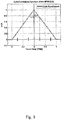
- Figure 13 schematically illustrates the Doppler Mis-Alignment Losses for the DSB and the SBP detector applied to BOC acquisition.
- Figure 13 represents the Doppler Mis-Alignment losses either for the DSB (sinc( ⁇ fd T int ) 2 ) or the SBP detector (sinc( ⁇ fd T int ) 2 ⁇ cos( ⁇ fd T int )) as function of the product ⁇ fd T int . It can be verified that the losses become larger when applying the SBP detector.
- ⁇ Rx 0 is therefore be set to 0, and does not appear in the following equations anymore.
- the SBP detector may be understood as an alternative detector to the previously described DSB detector.
- the detector output results from multiplying R Down Up ⁇ ⁇ , ⁇ f D with R Left Up ⁇ ⁇ , ⁇ f D (here a complex multiplication is applied), instead of adding the squared absolute values.
- the concept of the Sided Band Product detector for BOC-modulated signals is extended to the case of the Generalized-BOC-modulated signals, also called G-BOC, on the one side, and on the other side to the case of a G-BOC with asymmetrical data demodulation, G-BOC AS which can be compared to an Orthogonal Frequency Division Multiplexing (OFDM) signals.
- G-BOC Generalized-BOC-modulated signals
- OFDM Orthogonal Frequency Division Multiplexing
- Another combination of the elementary correlation functions of the elementary BOC(M k ,N k )-modulated signals can also be proposed in order to yield to a detector which is not sensitive to the ionosphere and hardware group delay.
- This alternative combination introduces the conjugate operator and can be considered as an extension of the conjugate SBP, D 1 , Conj SBP , introduced earlier for single BOC(M,N)-modulated signal.
- the SBP expression can be simplified by replacing each correlation contribution with the former n s 1 l t , n s 1 r t , n s 2 l t and n s 2 l t terms.
- E D 1 , Conj , GBOC AM SBP , 2 ⁇ ⁇ , ⁇ f D 2 E n s 1 l t ⁇ n s 1 r t ⁇ n s 2 l t ⁇ n s 2 r t ⁇ 2 + E n s 1 l t ⁇ n s 1 r t ⁇ ⁇ n s 2 l t ⁇ n s 2 + 2 ⁇ E n s 1 l t ⁇ n s 1 r t ⁇ n s 2 l t ⁇ n s 2 r t ⁇ + n s 1 l t ⁇ n s 1 r t ⁇ n s 2 l t ⁇ n s 2 r t ⁇ + n s 1 l t ⁇ n s 1 r t ⁇ ⁇ n s 2 l t ⁇ n s 2
- the definition of the SBP-Detector comprises multiplying the correlator outputs for the left side lobe with the correlator outputs for the right side lobe for each elementary BOC(M k ,N k )-modulated signal.
- the corresponding products are summed up to generate the aggregate detector output (SBP detector) for the Generalized BOC-modulated signal constituted of the K elementary BOC-modulated signals.
- SBP detector aggregate detector output
- the (Equation 83) provides the expression of the correlator output for the left R p k Left t and right R p k Right t side lobes, for the elementary BOC(M k ,N k )-modulated signal in the case of a time multiplexing scheme.
- the time multiplexing scheme it is necessary to account on top the time interval when each elementary BOC(M k ,N k )-modulated is active.
- a further extension of the Side Band Product detector covers the case of a G-BOC for which the lower and upper sideband signal do not contain obligatory the same symbol or data for each of the elementary BOC(M k ,N k )-modulated signals.
- This type of G-BOC is called G-BOC signal with asymmetrical data modulation and will be called G-BOC AS signal in the present disclosure.
- I represents the number of carrier frequencies.
- f i represents each carrier frequency.
- p i (t) is a pulse shape which modulates each carrier frequency.
- d i (t) is a data or symbol applied to each carrier frequency.
- data is used generically and can either correspond to symbols, when a coding scheme such as a Convolutional or a Turbo encoder is used to transform data into symbols, or to data when no encoder is applied.
- the complex factor ⁇ i ⁇ e j( ⁇ i) has the same signification and purpose as for the G-BOC-modulated signal.
- f u is a reference frequency used for the generation of the I elementary frequencies.
- DFT Discrete Fourier Transform
- GBOCAS GBOCAS
- the square operation is necessary to be immune against the data or symbol signs.
- each DFT( s GBOCAS ( t k ),i) component is multiplied with its symmetrical component DFT( s GBOCAS ( t k ) , I-i+1) with respect to the central frequency, i.e. carrier frequency.
Landscapes
- Engineering & Computer Science (AREA)
- Radar, Positioning & Navigation (AREA)
- Remote Sensing (AREA)
- Computer Networks & Wireless Communication (AREA)
- Physics & Mathematics (AREA)
- General Physics & Mathematics (AREA)
- Position Fixing By Use Of Radio Waves (AREA)
Description
- The present invention relates to a method and device for signal acquisition of a Generalized BOC-modulated signal.
- The first generation of GNSS signals (GPS and GLONASS systems) were modulated with the Binary Phase Shifted Keying (BPSK(N)) pulse shape, as for the GPS CA L1 signal using a BPSK(1). Here N designates the multiplicative factor which enables to derive the actual chip rate, fc, from a common reference frequency f0=1.023MHz, as follows fc=N×f0. The drawback of the BPSK pulse shape is an unsatisfactory code ranging performance. The always growing needs in accuracy for the final position solution asked for a new generation of pulse shapes which could offer an improved ranging accuracy. For this purpose, the so-called Binary Offset Carrier (BOC)-modulated signal has been introduced. The BOC(M,N)-modulated signal is obtained by multiplying an underlying BPSK(N)-modulated signal having a chip rate fc with a cosine or sinus function oscillating at a sub-carrier frequency, fsc=M×f0, and quantised over two levels, which explains the usage for the term "Binary". The BPSK pulse shape used for the generation of the BOC(M,N)-modulated signal is called primitive pulse shape. If no quantisation is applied onto the cosine or sinus function, then a so-called Linearly Offset Carrier (LOC)-modulated signal is obtained. Examples of BOC-modulated pulse shapes of current navigation signals are the BOC(10,5) of the Galileo E6-A signals, the BOC(15,2.5) of the Galileo E1-A or the BOC(10,5) of the GPS M signals. Other examples of pulse shapes for current navigation signals can also combine two elementary BOC-modulated signals, as for example the Galileo E1-B and E1-C signals, combining each a BOC(1,1) and a BOC(6,1), or the GPS L1C signal, also combining a BOC(1,1) and a BOC(6,1). Here, two different cosine or sinus functions having each different sub-carrier frequencies fsc1=M1×f0 and fsc2=M2×f0 are multiplied with the underlying BPSK(N1) and BPSK(N2), where N2 can be different or equal to N1, yielding two elementary BOC-modulated signals BOC(M1,N1) and BOC(M2, N2). The elementary BOC-modulated signals are each multiplied with a complex factor α×e-2πj((ϕ) and then recombined, either using a amplitude multiplexing scheme, meaning that the elementary BOC-modulated complex signals BOC(M1,N1)×α1×e-2πj(ϕ1) and BOC(M2,N2)×α2×e-2πj(ϕ2) are added, or using a time multiplexing scheme, meaning that segments of the elementary BOC-modulated complex signals BOC(M1N1)×α1×e-2πj(ϕ1) alternate with segments of the elementary BOC-modulated complex signals BOC(M2,N2)×α2×e-2πj((ϕ2). The relative power sharing of the two elementary BOC-modulated signals is achieved either by applying appropriate scaling amplitudes α1 and α2, in the case of amplitude multiplexing scheme, or by adapting the proportions between segments containing the elementary BOC-modulated complex signals BOC(M1,N1)×α1×e-2πj(ϕ1) and segments containing the elementary BOC-modulated complex signals BOC(M2,N2)×α2×e-2πj(ϕ2), in the case of timing multiplexing scheme. This example based on existing navigation signals can be extended to Generalized BOC-modulated signals, also called G-BOC, obtained by combining K elementary BOC-modulated signals either with an amplitude or a time multiplexing scheme, after having scaled them with complex factor αk×e-2πj(ϕk). In the special cases of the Galileo E1-B and E1-C, or GPS L1C K=2.
- The main consequence of the cosine or sinus multiplication is a wider spectral occupation. Due to this larger spectral occupation, the BOC signal offers a better immunity against multipath effects and thermal noise during tracking phase. The main draw-back of such signals is their Auto-Correlation Function (obtained by a matched replica) which contains several peaks which force to reduce the code binwidth (or equivalently the number of correlators) during the acquisition phase. This drawback is especially distinct for an acquisition of the BOC(15,2.5) signal of the Galileo E1-A.
- To prevent this situation, techniques have been developed and used to enlarge a main peak of the correlation function (no more obtained by a matched filter) but at the cost of larger squaring losses which force a higher C/N0 requirement.
-
US 2004/071200 A1 disclosess signals processing architectures for direct acquisition of spread spectrum signals using long codes. Techniques are described for achieving a high of parallelism, employing code matched filter banks and other hardware sharing. In one embodiment, upper and lower sidebands are treated as two independent signals with identical spreading codes. Cross-correlators, in preferred embodiments, are comprised of a one or more banks of CMFs for computing parallel short-time correlations (STCs) of received signal samples and replica code sequence samples, and a means for calculating the cross-correlation values utilizing discrete-time Fourier analysis of the computed STCs. One or more intermediate quantizers may optionally be disposed between the bank of code matched filters and the cross-correlation calculation means for reducing word-sizes of the STCs prior to Fourier analysis. The techniques described may be used with BOC modulated signals or with any signal having at least two distinct sidebands. - Therefore, the present invention is intended to solve the technical problem of significantly limiting the corresponding squaring losses.
- The present invention is defined by the independent claims. Specific embodiments are defined by the dependent claims.
- According to a first aspect of the present invention, a method for signal acquisition of a Generalized Binary Offset Carrier, G-BOC, modulated signal comprising K elementary BOC(Mk,Nk)-modulated signals is provided, as defined by
independent method claim 1. - For example, the detector output may indicate detection when the detector output is equal to or higher than the detection threshold.
- Herein, the term hypothesis may also be understood as test hypothesis. BOC-modulated can mean the usage of a BOC pulse shape. The BOC-modulated signal can be modulated with symbols/data. If it is not modulated with symbols/data, then it serves as pilot signal. Herein the terms "detector" and "detector output" can be used interchangeably.
- One of the main consequences of this disclosure is that the detector output can be made independent from a symbol included in the data modulated on the BOC-modulated signal. This has the advantage of improving acquisition performance for data modulated signals using a BOC pulse shape.
- The detection threshold can be set to a probability of false alarm or a probability of missed detection.
- The step of correlating can comprise a coherent integration. For conventional acquisition the coherent integration can be performed over a time duration which is limited by the duration of the symbols or data which can be modulated onto the G-BOC-modulated signal. The coherent integration can be performed over a time duration being equal or lower than a symbol duration, when symbols or data are included in data modulated on the G-BOC-modulated signal. For typical GNSS signals the symbols are derived from the data bits of information using a dedicated coding scheme such as a convolutional coding scheme. In comparison to conventional acquisition, the proposed disclosure enables to discard the constraint regarding the symbol or data duration onto the coherent integration time. For G-BOC-modulated signals which do not comprise symbol or data, no constraint related to symbol or data modulation applies to the time duration of the coherent integration.
- The time duration for the coherent integration time can also depend on the dynamic of a link between a transmitter and a receiver. The transmitter can be a space-based or terrestrial GNSS or a RNSS transmitter. The receiver can be a space-based or terrestrial GNSS or a RNSS receiver respectively. Typical terrestrial RNSS transmitters are called Pseudolites. The dynamic of the link between a space-based transmitter and a terrestrial or space-based receiver is usually large, and the resulting Doppler can limit the maximal tolerated coherent time duration. The dynamic of a link between a terrestrial transmitter and a terrestrial receiver is usually much smaller, and the coherent time duration can be much longer.
- A hardware group delay and/or a carrier delay can be estimated and included in the complex multiplication. The carrier delay can be based on an ionospheric effect.
- It is possible that only the real part of the detector output indicates detection.
- It is also possible that only a positive detector output is compared to the detection threshold and a negative detector output is discarded or ignored, for example for the step of comparing with the detection threshold.
- The G-BOC-modulated signal can comprise K sub-carriers. The K sub-carriers can be multiplexed either with an amplitude or a time multiplexing scheme. Each of the K sub-carriers can be modulated with data or not. When a sub-carrier fsc,k is modulated with data, the data or symbol contained in the lower sideband signal corresponding to the elementary sub-carrier fsc,k can be identical or different to the data or symbol contained in the upper sideband signal corresponding to the elementary sub-carrier fsc,k. At the generation of the G-BOC modulated signal, when the data is multiplied in the time domain with a cosine, cos(2πfsc,kt) or a sinus sin(2πfsc,kt) term operating at sub-carrier frequency fsc,k, then an identical data is contained in the upper and lower side-band signals. The data contained in the lower and upper sideband signals corresponding to the elementary sub-carrier fsc,k can be different when, at the generation of the G-BOC modulated signal, the data which is multiplied in the time domain with an exponential exp(-2πfsc,kt) standing for the lower side-band signal is different to the data which is multiplied in the time domain with an exponential exp(+2πf sc, kt) standing for the upper side-band signal.
- The data can be modulated onto the G-BOC signal by multiplying the data modulated pulse shape either with a cosine or a sinus function yielding to the same data on the upper and lower sideband signals of a sub-carrier frequency fsc,k, or by multiplying the data modulated pulse shape with an exponential function to modulate different data on the upper and lower sideband signals of a sub-carrier frequency fsc,k.
- In particular when the G-BOC-modulated signal is modulated with I =2xK data symbols, a number of symbols or data can correspond to the number of carriers I. The two data symbols corresponding to each of the K sub-carriers can be identical or different. Each of the I carriers can have merely one symbol. A time-frequency domain pattern of the I symbols or data can be symmetrical to a central carrier of the G-BOC-modulated signal. When the time-frequency domain pattern is not symmetrical then the corresponding signal is referred to as Generalized BOC with asymmetrical data demodulation, and can be compared to an Orthogonal Frequency Division Multiplexing. In the case of K=1 sub-carriers, each symbol can be spread with one spreading sequence. In the case of K>1 subcarriers, each symbol can have a same duration as one chip of the BOC-modulated signal.
- The I symbols can correspond to I Fourier components determined by a Discrete or Fast Fourier Transform. The step of combining can comprise complex multiplication of the Fourier components.
- The I symbols can correspond to I Fourier components forming an asymmetrical time-frequency pattern determined by a Discrete or Fast Fourier Transform. The step of combining can comprise selecting pairs of the I symbols over time such that their values is identical and their frequencies are symmetrical to the central carrier of the G-BOC-modulated signal. Further, the step of combining can comprise multiplying the selected pairs with a correction factor accounting for the time offset between each of the selected pairs. Further, the step of combining can comprise complex multiplying the corrected I Fourier components.
- According to a second aspect of the present invention, a computer program which when carried out on a processor of a device for signal acquisition of a generalized binary offset carrier, G-BOC, causes the processor to carry out the method according to the first aspect is provided.
- According to a third aspect of the present invention, a storage device storing a computer program according to the second aspect is provided.
- According to a fourth aspect of the present invention, a device for signal acquisition of a Generalized Binary Offset Carrier, G-BOC, modulated signal comprising K elementary BOC(Mk,Nk)-modulated signals is provided, as defined by independent device claim 14.
- The present invention offers significant advantages w.r.t. a Double Side Band, DSB, method, for applications 1) with limited effects from the ionosphere and 2) with low dynamic of the emitter-receiver link (transmitter-receiver link).
- Even if the foregoing described aspects with respect to the method were only described for the method, these aspects can further relate to the foregoing described device and vice versa.
- The present invention will be further described in more detail hereinafter with reference to the figures.
- Figure 1
- schematically illustrates a GNSS receiver;
- Figure 2
- schematically illustrates an acquisition scheme for Binary Phase Shift Keying, BPSK, signals;
- Figure 3
- schematically illustrates an Auto-Correlation Function, ACF, for a BPSK(2.5) pulse shape;
- Figure 4
- schematically illustrates an acquisition scheme for Binary Offset Carrier, BOC, signals;
- Figure 5
- schematically illustrates an Auto-Correlation Function (ACF) for a BOC(5, 2.5) signal;
- Figure 6
- schematically illustrates a Dual Side Band, DSB, acquisition scheme;
- Figure 7
- schematically illustrates the detector output for the DSB acquisition according to the scheme presented in
figure 6 ; - Figure 8
- schematically illustrates an acquisition scheme according to an embodiment of the present invention;
- Figure 9
- schematically illustrates a dwell time diagram for a non-coherent integration time and for a varying coherent integration time for a SBP detector;
- Figure 10
- schematically illustrates squaring losses due to the non-coherent summations for mitigation of symbol flips;
- Figure 11
- schematically illustrates a R.O.C. Curve for a BOC(5,2.5) signal;
- Figure 12
- schematically illustrates a R.O.C. Curve for a BOC(15,2.5) signal;
- Figure 13
- schematically illustrates Doppler Mis-Alignment Losses for the DSB and the SBP detector applied to BOC acquisition;
- Figure 14
- schematically illustrates power spectral density, PSD, of the BOC(5,2.5) and intermediate signal used for DSB and SBP detector;
- Figure 15
- schematically illustrates the absolute value of the Matched Filter, DSB and SBP detector (BOC(5,2.5));
- Figure 16
- schematically illustrates the power spectral density, PSD, of the BOC(15,2.5) and intermediate signal used for DSB and SBP detector;
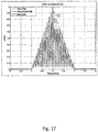
- Figure 17
- schematically illustrates the absolute value of the Matched Filter, DSB and SBP detector for (BOC(15,2.5));
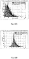
- Figure 18A
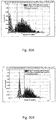
- schematically illustrates a distribution for the DSB in the "H0" and "H1" hypotheses for BOC(15,2.5) for 25 dB-Hz;
- Figure 18B
- schematically illustrates a distribution for the SBP Detector in the "H0" and "H1" hypotheses for BOC(15,2.5) for 25 dB-Hz;
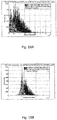
- Figure 19A
- schematically illustrates a Distribution for the DSB in the "H0" and "H1" hypotheses for BOC(15,2.5) for 30 dB-Hz;
- Figure 19B
- schematically illustrates a Distribution for the SBP Detector in the "H0" and "H1" hypotheses for BOC(15,2.5) for 30 dB-Hz;
- Figure 20A
- schematically illustrates a distribution for the DSB in the "H0" and "H1" hypotheses for BOC(15,2.5) for 35 dB-Hz;
- Figure 20B
- schematically illustrates a Distribution for the SBP Detector in the "H0" and "H1" hypotheses for BOC(15,2.5) for 35 dB-Hz;
- Figure 21
- schematically illustrates a Model for the SBP detector output in the "H0" and "H1" hypotheses;
- Figure 22
- schematically illustrates the sequencing of the spreading codes involved in the generation of a Generalized BOC signal using an time multiplexing, with K = 3 elementary BOC(Mk,Nk) signals;
- Figure 23
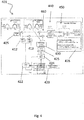
- schematically illustrates a scheme applied for the acquisition of a Generalized BOC signal with K =2 and according to an embodiment of the present invention;
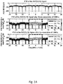
- Figure 24
- schematically illustrates the independency of the four noise contributions involved in the calculation of the generalized SBP detector applicable to a Generalized BOC modulated signal with K=2;
- Figure 25
- schematically illustrates the generation of a G-BOCAS signal;
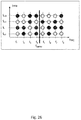
- Figure 26
- schematically illustrates a Time-Frequency Domain Pattern of Modulated Symbols of a G-BOCAS signal;
- Figure 27
- schematically illustrates a Time-Frequency Domain Pattern of Modulated Symbols of a G-BOCAS signal according to an embodiment of the present invention; and
- Figure 28
- schematically illustrates a Time-Frequency Domain Pattern of Modulated Symbols of a G-BOCAS signal according to an embodiment of the present invention.
-
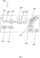
Figure 1 schematically illustrates aGNSS receiver 100. Here, the main functional blocks are briefly discussed. A signal can be received via anantenna 105, which is then fed to apre-amplifier stage 110, whose aim is to increase the received signal to a level (voltage) compatible with the following functional blocks of the receiver front-end. Thepre-amplifier stage 110 can comprise a single or several amplifiers mounted in cascade, and the first amplifier called Low Noise Amplifier (LNA) is usually characterised by a small Noise Figure (NF). The signal in an RF domain, for example 1575.42 MHz for the Galileo E1-B signal, is first down-converted to an Intermediate Frequency (IF). This down-conversion is usually performed in analogue by the Down-Converter 115 before the Analogue to Digital Converter, A/D Converter 120, but could also be performed in a digital domain, if the sampling frequency of the A/D Converter 120 is large enough following Nyquist condition. To perform down-conversion, the signal in the RF domain is multiplied with a cosine having a frequency (IF-RF), for example IF-1575.42 MHz. The frequency (IF-RF) is generated via aFrequency Synthesizer 113 driven by aReference Oscillator 112. Then the down-converted signal being in an IF domain is sampled by the A/D Converter 120. It is usual to call the part before the A/D Converter 120, the "Analogue Front-End" and the part following the A/D Converter 120 the "Digital Front-End". In order to adapt the power of the received signal in near real time, an Automatic Gain Control,AGC 122, monitors a power level of the samples and provides an information to multiply the received signal in the RF domain with a variable gain, for example into the Down-Converter 115 as illustrated in thefigure 1 . Finally, the output of the A/D Converter 120 is fed to a blanker 180 whose aim is to set the samples, which contain pulsed interferences with high power on top of the received signals, to e.g. 0. Infigure 1 the blanker 180 is implemented in the digital front-end, but in other receiver implementations, the blanker 180 can be implemented in the analogue front-end. After blanking, the digital samples are then provided to QDigital Receiver Channels 130, where Q represents the number of line-of-sight transmitter signals, for example satellite signals, necessary to be tracked in order to calculate a position, with a required position and timing performance. Usually, the more channels exist the better the position accuracy. Each of the QDigital Receiver Channels 130 aims at processing the signal in the IF domain by first wiping-off the remaining carrier frequency IF, and by providing the different correlator channels, which are necessary for signal acquisition but also for a code and carrier estimation and navigation data demodulation. The present invention focusses on acquisition processing. The aim of the acquisition of a CDMA signal is to coarsely estimate the code delay and the Doppler frequency of the received signal. The estimated code delay and Doppler frequency are usually called code (delay) and Doppler (frequency) hypotheses respectively. For this purpose, a set of code delay hypotheses and Doppler frequency hypotheses is tested. For each pair of code delay/Doppler frequency hypotheses a replica is firstly generated by shifting the spreading sequence with the corresponding code delay and multiplying this shifted sequence with a carrier modulated at the Doppler frequency hypothesis. Then the received signal is correlated with the replica generated for the code delay and Doppler frequency hypotheses. Finally, the corresponding correlation is squared to build the acquisition detector, which is an equivalent to a power estimator. This detector output is compared to a threshold either set according to a desired Probability of False Alarm (PFA) caused by unavoidable thermal noise and possibly combined with correlation contributions from other received signals different from the one to be acquired, or set according to a probability of missed-detection (PMD). A situation called a cold start exists, when no information about the code delay and Doppler frequency of the received signal is available. All code delay hypotheses corresponding to the whole spreading sequence have to be searched. Typical order of magnitude for the code delay to be searched corresponds to the spreading code duration, for example 1ms (equivalent to the 1023 chip sequence) for the GPS C/A signals and 4ms for the Galileo E1-B and (equivalent to the 4092 chip sequence).Typical order of magnitude for the Doppler to be searched is ±10 KHz. To limit the combined Code and Doppler mis-alignment losses during the correlation process to a few dBs, usually 1 to 3 dB, one code delay hypothesis is usually tested every Tc/2 or Tc/4, where Tc is the chip duration, and one Doppler hypothesis is tested every 50 to 100Hz. As an example for a GPS C/A signal having a spreading sequence containing 1023 chips, at least 2046 code delay hypotheses can be tested. Those sampling intervals for the code delay and Doppler frequency hypotheses are called respectively Code and Doppler binwidths. In order to improve the performances for the acquisition process, it is possible to add non-coherently the detector outputs for successive correlations of the received signal with the replica generated with the same Code delay and Doppler frequency hypothesis to be tested. Due to the non-coherent summations, so called squaring losses have to be taken into account. To avoid such squaring losses, it is possible to increase a coherent integration time. The coherent integration is one configuration parameter for computing the correlation of the received signal with the replica. The replica and received signals can be correlated over a longer correlation time, but in that case the Doppler mis-alignment losses increases. The appropriate configuration setting of the acquisition scheme, such as code delay and Doppler binwidths, coherent correlation time, number of non-coherent summations, PFA and PMD rate, etc., depends on a choice of a receiver manufacturer. For BPSK signals, the acquisition scheme is further explained infigure 2 . -
Figure 2 schematically illustrates an acquisition scheme for Binary Phase Shift Keying, BPSK, signals, formerly explained and based on a digital receiver channel introduced infigure 1 . A BPSK(N) designates a Binary Phase Shift Keying modulation for the chips, with a chip rate, fc, equal to fc=N×f0, where N designates the multiplicative factor applied to the common reference frequency f0=1.023MHz. Typical BPSK signals are the GPS L1 C/A with a BPSK(1) and the GPS L5 signals with a BPSK(10). A received signal in the IF domain provided by the functionalblock Digital IF 205 is separated into an in-phase component and a quadrature component via a respective cosine and sine function provided by theCos Map 212 and theSin Map 213 by use of aCarrier NCO 222 which is offset by aDoppler frequency hypothesis 220. Both in-phase and quadrature components are then correlated with a replica generated on the basis of a code delay hypothesis via aCode NCO 224 and aCode Generator 225. The correlation comprises a step ofcoherent integration 240. For signal detection, anincoherent integration 250 is performed for each of the correlation results. Thisincoherent integration 250 comprises the step of squaring of the correlator outputs of the in-phase and quadrature components and the step of summing and combining the NNC squared outputs of the in-phase and quadrature components. NNC designates the number of non-coherent summations. The results are summed up to form, DMF,
acquisition processor 235. A respective Correlation result for an exemplary BPSK signal is shown infigure 3 . -
Figure 3 schematically illustrates an Auto-Correlation Function (ACF) for a BPSK(2.5) pulse shape, which is used to detect the presence of the signal for the Code delay and Doppler frequency hypotheses. In this illustrative example, two hypotheses per chip are tested, each highlighted as dark lines at ±0.25 and ±0.75 chip on the X-axis. Further, the replica infigure 3 has Zero-Doppler mis-alignment. The figure also highlights the worst case alignment between the actual position of the correlation function and code hypothesis grid. Here the Code-Misalignment losses (2.5dB = -20∗log(0.75)) are therefore evaluated for the code delay of Tc/4. -
Figure 4 schematically illustrates an acquisition scheme for Binary Offset Carrier, BOC, signals. The new generation of GNSS signals, for example in systems like Galileo, GPS, COMPASS, a pulse shape modulation, called BOC(M,N) is used. For example, the Galileo PRS signals are modulated with a BOC(10,5) for the E6-PRS signals and a BOC(15,2.5) for the E1-PRS signals, and GPS M-signals are modulated with a BOC(10,5). BOC(M,N) signals have a chip rate of N×1.023 MCps and a so-called sub-carrier at M×1.023 MHz. This BOC(M,N) pulse shape is generated by multiplying the spreading sequence modulated with a primitive BPSK(N) pulse shape having the chip rate, fc, of N×1.023 MCps with a cosine or sinus function oscillating at a sub-carrier frequency, fsc, at fsc=M×1.023 MHz frequency, and digitised with one bit, only +1 and -1 levels, which is referred to as "binary". If no quantisation is applied onto the cosine or sinus function, then a so-called Linearly Offset Carrier (LOC)-modulated signal is obtained. The main consequence of the application of sub-carrier is that the spectral representation of a BOC(M,N) has two main side-lobes distant of +M×1.023 MHz and -M×1.023 MHz with respect to the central carrier frequency, while the spectral representation of a BPSK(N) signal has a single main lobe at the central carrier frequency. BOC(M,N) signals are known to be more robust against thermal noise and multipath effects, when considering tracking performances. This is due to their wider bandwidth directly depending on M. When considering acquisition performances, it could also be possible to apply a matched filter acquisition strategy already proposed for the BPSK modulated signal infigure 2 . This matched filter acquisition strategy is presented onfigure 4 for BOC-modulated signals with its respective functional blocks. -
Figure 5 schematically illustrates an Auto-Correlation Function (ACF) for a BOC(5, 2.5) signal. If one applies the same acquisition scheme for a BOC signal according tofigure 4 as for the BPSK signal according tofigure 2 , namely a matched filter replica, where the replica uses a BOC pulse shape, then the central peak of the correlation function becomes narrower. This is illustrated onfigure 5 for the special case of a BOC(5,2.5) signal. It can be effectively observed that for the same Code Mis-alignment losses (2.5 dB = -20∗log(0.75)), the code binwidth becomes 4 times smaller, and therefore the number of code hypotheses becomes 4 times larger. This affects the number of dark lines illustrated infigure 5 on the X-axis. Further, the replica infigure 5 has Zero-Doppler mis-alignment. If one considers a BOC(M,N) where the ratio between the chip rate (N×1.023 MCps) and the sub-carrier (M×1.023 MHz) is higher, as for example the BOC(15,2.5) of the Galileo E1-A signals, then the binwidth becomes even smaller for the same mis-alignment losses, which can concretely lead to an unacceptable number of hardware correlators. Infigure 5 , the exemplary binwidth ensuring 2.5dB of Code mis-alignment losses is Tc/8 instead of Tc/2 as in the case of the BPSK(2.5) signal. To avoid such a situation, there is an alternative and well-recognized acquisition method shown infigure 6 . -
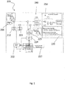
Figure 6 schematically illustrates a Dual Side Band, DSB, acquisition scheme. For the "left spectral side lobe", the respective lower spectral sideband of the BOC signal, the input BOC signal is up-converted, for example by multiplication with an exponential which is itself generated by asub-carrier generator 680, and then filtered with a Low Pass (LP) Filter atbaseband 670, before being correlated with a replica modulated with a BPSK(N) pulse shape having the same chip rate, N×1.023 MCps, as the BOC signal and also the same spreading sequence, leading to the CCFLeft correlation function, namely
correlation 640 for "left spectral side lobe" of the BOC signal is used for acquisition. Herein the in-phase and quadrature components of the correlator are squared and summed to form the non-coherent correlation a CCFLeft = |CCFIn |2 + |CCFQuad |2 . By summing non-coherently NNC such successive non-coherent correlations,
sub-carrier generator 680,second LPF 670 and third correlation with a BPSK(N) replica 640), leading to the CCFRight correlation function, namely


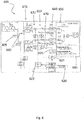
figure 7 . -
Figure 7 schematically illustrates the square root detector output (shown asline 711 infigure 7 ) for the DSB acquisition according to the scheme presented infigure 6 . The corresponding square root of the detector,


- Tint represents the coherent integration time. εfd represents a Doppler estimation error between the true Doppler and its tested value. Δτ represents a Code estimation error between the true Code delay and its tested value. τGD represents a hardware group delay. τiοnο represents a delay caused by the ionosphere. As for the acquisition of the BPSK(N) signal it is possible to add non-coherently

-
Figure 8 schematically illustrates an acquisition scheme according to an embodiment of the present invention. If the number of code delay and Doppler frequency hypotheses can be reduced by use of the DSB approach, one identified drawback is the larger squaring losses. Furthermore, by squaring the corresponding detector outputs an additional and degrading contribution comes from a variance of the thermal noise (and interferences). It means that even if the wrong code delay and Doppler frequency hypotheses are proposed, the distribution of the DSB detector output has not a zero-average but an average depending on the noise variance, and which can degrade the probability of false alarm. - To circumvent both degrading effects, it is therefore proposed to process the correlator outputs for "Left-Sided" and "Right-Sided" Spectral Lobes (lower and upper sideband) of the BOC signals in a different way than for the SSB or DSB schemes. Here, both correlations are no more squared and added (|CCFLeft|2 + |CCFRight|2), but are multiplied with each other:


- ϕRx GD represents the effect of the hardware group delay onto the carrier. ϕiono represents the carrier delay caused by the ionosphere. By applying this alternative definition of the detector output for the BOC signals the following advantages can be identified:
- In case the BOC-modulated signal is modulated with symbols or data, because both left and right side lobes are modulated with the same symbol (GNSS data), by multiplying CCFLeft and CCFRight the corresponding detector DSBP does not depend on the symbol any more. Assuming no noise, the sign of DSBP would be always positive. It means that in presence of noise, only half of the detector distribution shall be investigated. With thermal noise, it also means therefore that all positive values of the detector output could be accounted. It means that the setting of the detection threshold w.r.t. the false alarm rate, can be based on the positive part of the detector values even if the DSBP takes both positive and negative values.
- The GPS M signals, Galileo E1-A (PRS), E6-A (PRS) or the Galileo (OS) signals (this later signal uses the combination of a BOC(1,1) representing 10/11 of the aggregate power and a BOC(6,1) having 1/11 of the aggregate power and is categorized in the "Generalized BOC-modulated signals" described herein), are modulated with data/symbols. For example the E1-B OS signal is a data channel with symbol duration of 4ms. As a consequence, it is not possible to integrate coherently over a time duration larger than the symbol duration, since the symbol flips with a 50% occurrence might lead to a total collapse of the correlation output calculated over a coherent integration time spreading over more than 1 symbol. By using the acquisition scheme according to the embodiment of the present innovation according to
figure 8 , this constraint does not apply anymore, because the new detector output DSBP is not affected by the symbol (immune to the symbol effect). Therefore, it is possible to integrate coherently over a much longer time duration. A possible limitation applying to the maximal time duration for the coherent integration is driven by the dynamic of a Transmitter-Receiver Link. This limitation is higher for Satellite-based GNSS, but this limitation becomes much smaller for Terrestrial RNSS applications, for example for Pseudolites. Therefore, for terrestrial systems using CDMA signals, modulated with BOC pulse shapes, acquisition can be performed by integrating over a much longer coherent integration time, and especially for data modulated signals. - Because a LPF has been applied for the generation of the CCFLeft and CCFRight before the correlation process, the corresponding additive noise contributions of the CCFleft and CCFRight can be considered as independent. As a consequence the average of the new detector output DSBP does not depend on noise power, as for the Dual Side Band detectors, and the corresponding distribution of the Side Band Power detector is evenly centred. Again, this is not the case when applying the standard DSB acquisition scheme. This is due to fact that the average of the DSB detector output directly depending on the noise variance (see explanation for
figure 6 ). - For applications, where the transmitter is a satellite, if the RF-link crosses atmospheric layers with high ionospheric activity (for a corresponding RF carrier frequency), then it is shown that the value of the detector output DSBP contains a multiplicative, and a complex factor which depends on the ionosphere (e j(2ϕiono)), as observed in (Equation 2). The ionosphere leads to a delay which applies to the phase of the complex signal, and depends on the Total Electron Content (TEC) of the link crossing the ionosphere. This multiplicative term prevents the possibility to test only the real part of the detector output DSBP. It must be highlighted that the ionosphere leads to another delay affecting the code, which is also observed for the conventional DSB detector (see (Equation 1) and (Equation 2)). For links which do not cross the ionosphere, or an RF-links for which the delay caused by the ionosphere is negligible for the specific carrier frequency, then the multiplicative term does not exist or is negligible, and it is possible to only compare the real part of the detector output DSBP with a threshold set according to a specified PFA or PMD level. To circumvent the effect of the ionosphere, either a ionosphere delay on the carrier can be considered as negligible (e j(2ϕiono) ≈ 1) or an estimation of the ionosphere delay, ϕ̂iono , is subtracted from a true ionosphere delay on the carrier. The residual can again be considered as negligible: e j2(ϕiono- ϕ̂ iono) ≈ 1. (Equation 2) shows that the value of the detector output DSBP also contains a multiplicative, and complex factor which depends on the hardware group
delay 
negligible 


figure 8 , an additional input to theacquisition block 835 is introduced to account for the combined tested group delay and ionospheric delay. From (Equation 2), it is shown that the analytical expression for the detector output DSBP contains an additional complex and multiplicative term which is a function of the Doppler mis-alignment
term 
term 
- It appears that the present invention offers significant advantages w.r.t. the DSB method, for applications 1) with limited effects caused by the ionosphere and 2) with low dynamic of the transmitter-receiver link, for example applications with terrestrial transmitters and receivers (even mounted on a platform) with reasonable dynamic. Another possible use of the proposed innovation is covered by indoor applications where transmitters are pseudolites. As far as the effect of the hardware group delay is concerned, this one shall be either negligible, or the calibration error shall be limited.
- For such indoor systems, it could be envisaged to apply the SBP detector for the acquisition of the signals having the same structure as the Galileo E1-B signals, meaning a data modulated signal, with a BOC(1,1) (combined with a BOC(6,1)) and a symbol rate of 4ms. In order to ensure satisfactory PMD and PFA levels at low carrier-to-noise ratio (C/N0) which is an actual situation for indoor applications, it is necessary to extend the integration time over many symbols. Now, to annihilate the degrading effects of the symbol changes for an extended coherent integration, a conventional acquisition strategy comprises summing non-coherently the elementary DSB detector outputs calculated over 4ms. For the application of the SBP detector it is possible to simply extend the coherent integration over the 4ms symbol transitions. This enables to significantly improve the acquisition sensitivity, which is advantageous when the received signal power is attenuated by the walls as for indoor applications. It is shown below that the Receiver Operational Curves (R.O.C), which relates the PFA as function of the PMD for a varying detection threshold, almost overlap for a coherent integration time of 4ms.
-
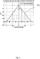
Figure 9 schematically illustrates a dwell time diagram for a non-coherent integration time and for a varying coherent integration time for the SBP detector. The dwell time is defined as the product of the number of non-coherent summations with the duration of the coherent integration, and represents the aggregate coherent and non-coherent time needed to ensure that both required PFA and PMD probabilities are fulfilled. By extending the dwell time either for the DSB detector, or for the SBP detector to ensure the same PFA and PMD levels, the resulting dwell time becomes smaller for the SBP detector than for the DSB.Figure 9 illustrates the required dwell-time necessary to ensure a PFA = 0.001 and a PMD = 0.9 either for a 4ms coherent integration used for both DSB and SBP detector cases (in the case of the DSB only non-coherent summations of 4ms are applied) or for coherent integration times, exceeding the symbol transitions, with 8ms, or 20ms or 40ms, ..., or 200ms (for the SBP detector). From this figure the degrading effects of the so-called squaring losses due to the non-coherent summation of the 4ms coherent integration can be deduced, which is represented onfigure 10 . -
Figure 10 schematically illustrates the squaring losses due to the non-coherent summations which can be used for mitigation of symbol flips when applying the DSB acquisition scheme. As a consequence, for very low C/N0 levels as those experienced in indoor, it is posssible to gain around 5 dB to 7dB for (C/N0) around 15 dB-Hz (typical in Indoor scenarios), and to work at a reasonable dwell time around 200ms, which is reasonable for transmitter receiver links with low dynamic . - In order to improve the detection performances of the SBP detector, it is proposed to modify the decision strategy, by remarking that the expected value of the detector output is positive when the correct corresponding Code and Doppler frequency hypotheses are tested ("H1" case). This alternative detection strategy can be summarised as follows:
- If the detector output is positive and is above the detection threshold, the "1" ("hit") is allocated.
- If the detector output is positive and is below the detection threshold, the "0" ("discard") is allocated.
- If the detector output is negative then no decision is taken, the SBP detector output is discarded, and another evaluation of the detector output for the same Code and Doppler frequency hypotheses is performed.
- For a comparison of this alternative SBP detector strategy, it is important to state that by introducing consecutive tests (for the "negative SBP detector outputs"), a decision is delayed, and therefore the Mean-Time-To-Acquire (MTTA) too. Here a rough evaluation of this impact comprises a multiplication with a factor 1.5 with the MTTA obtained without discarding the negative SBP detector outputs (since on average, 50% of the SBP detector outputs are negative for "H0" case, which mainly impacts the MTTA). The improvement brought by this alternative decision strategy is evaluated based on Monte-Carlo simulations. Undertaken Monte-Carlo simulations resulted in a Receiver Operational Curve (R.O.C.) which provides the Probability of Detection as function of the Probability of False Alarm.
-
Figure 11 and12 schematically illustrate R.O.C. Curves for BOC(5,2.5) and BOC(15,2.5) respectively for different values of the input (C/N0) ratios. Here the contributions of the ionospherical effect (ϕionο=0), receiver group delay ((ϕRx GD=0) and Doppler (εfd=0) are not considered, and only Code estimation error Δτ and thermal noise are accounted for the R.O.C determination. A coherent integration of 4ms was applied. From the R.O.C. curves, the following statements can be derived: - No (major) difference in performance exists between the DSB and the SBP detector (the SBP detector using both positive and negative outputs). At 25 dB-Hz, it is observable that the R.O.C. of the DSB and SBP detectors are almost overlapping (and crosses around the point (PFA=0.5, PD=0.7)). For larger C/N0 almost no difference exist neither. This means that a factor of 2 in amplitude which is lost in the SBP detector amplitude w.r.t. DSB one


- Now, the main advantage of the SBP detector resides in the possibility to integrate over a much longer coherent integration time when compared to the DSB, and this enables to overcome squaring losses.
- By applying the alternative detection strategy based on the SBP detector, but focusing only onto the "positive SBP detector outputs" (dashed line on
figures 11 and12 ), then an improvement of the R.O.C. performances is achieved. Again, this improvement of detection performance comes along with a ∼50% larger MTTA as stated above. - It is further described, how to derive and describe the mathematical models for the detector output, in order to justify the improvements in acquisition performances, obtained by the SBP detector according to an embodiment of the present invention. The influence of the ionosphere and receiver onto the code (group) delay and carrier offset affecting the elementary correlation outputs for the left and right side lobes of the BOC(M,N) power spectral density, PSD, is analysed. The corresponding derivation can help to introduce and justify an expression for the detector output according to an embodiment of the present invention, which is insensitive to such effects. For this purpose, a noise free environment is firstly considered. Then, the appropriate expression of the new detector output is derived, the effect of the noise is accounted, and especially the better immunity of the SBP detector against noise is explained.
-
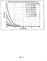
Figure 13 schematically illustrates the Doppler Mis-Alignment Losses for the DSB and the SBP detector applied to BOC acquisition.Figure 13 represents the Doppler Mis-Alignment losses either for the DSB (sinc(εfdTint)2) or the SBP detector (sinc(εfdTint)2 × cos(εfdTint)) as function of the product εfdTint. It can be verified that the losses become larger when applying the SBP detector. The following table provides the maximal Doppler error in the tested Doppler hypotheses (half of the Doppler binwidth), also called Doppler residual on the figure, and tolerated to not exceed Doppler mis-alignment losses of 1 or 2 dB.1 dB of Doppler Mis- Alignment Losses 2 dB of Doppler Mis-Alignment Losses εDopp [Hz] DSB εDopp [Hz] SBP Ratio εDopp [Hz] DSB εDopp [Hz] SBP Ratio 262 98 2,7 366 134 2,7 66 25 2,6 92 34 2,7 27 10 2,7 37 14 2,6 14 5 2,8 19 7 2,7 - The Doppler error shall be approximately 2.7 times smaller when applying the SBP detector, when compared to the DSB. It means that the dynamic of the Transmitter-Receiver link can represent a higher limitation for the acquisition when using the SBP detector. For applications with terrestrial transmitters and a receiver mounted on a platform with reasonable dynamic, this limitation can be regarded as acceptable. This would be for example the case for Indoor applications.
- In the following, a Detector Output Expression is derived when accounting carrier, code and group delays due to the ionosphere and the receiver, but without accounting for the thermal noise (Noise-Free Environment). The expression of the received signal at RF and using complex notations is given by:

- Px represents a received power. fcarr is a central carrier frequency (e.g. 1575.42MHz). fD is a Doppler offset according to radial velocity. ϕiono is a contribution to the carrier phase offset caused by the ionosphere, which can be rewritten to:

ϕRx 0 is an initial phase of the carrier at reception and which is usually depending on an initial phase ϕTx 0 at signal generation, on-board the satellite for example, and which is itself unambiguously defined. A typical value assignment for ϕTx 0 is zero which means that the zero-crossing of the carrier wave corresponds to a front-edge of a chip, yielding a so-called Code-Carrier Coherency. It means that the hardware contribution of the generation chain ϕTx GD at satellite level needs to be specified to ensure that ϕTx 0 stays equal to zero or close to zero over the range of on-board temperature variations. Because the impacts of the ionospherical effects (with ϕiono), the receiver hardware (with ϕRx GD) and the Doppler (fD×(t-τ)) are accounted into the carrier phase, the initial phase ϕRx 0 at reception can be then identified to the initial phase ϕTx 0 at transmission. Other unambiguous definitions of the initial carrier phase ϕTx 0 can also be proposed, but the principle would remain and again ϕRx 0 could be identified to ϕTx 0 meaning that ϕRx 0 is also known at reception side, and does not correspond to a parameter to be estimated during the acquisition process, as it is the case for the code delay τ and the Doppler offset fd. In the following ϕRx 0 is therefore be set to 0, and does not appear in the following equations anymore.
- τRx GD is a contribution to the code phase offset from the receiver hardware. c(t) is a spreading code sequence. d(t) is a symbol which is modulated (spread) with the spreading sequence c(t). In this expression the spreading sequence can be periodical as for the Galileo E1-B with a period of 4ms, or non-periodical. Furthermore, when it is periodical the spreading sequence period usually corresponds to one symbol duration. In the absence of a modulated symbol such as for the pilot Galileo E1-C signal, the term d(t) does not exist. pBOC is a pulse shape corresponding to a BOC(M,N) modulation, with sub-carrier fsc (15×1.023MHz for the Galileo L1-A PRS signals), and is expressed as

- In this expression a cosine function, cos(2πfsc (t), has been applied to generate the pulse shape pBOC(t). A similar expression for the pulse shape pBOC(t) can be derived when apply a sinus function, sin(2πfsc (t), in place of the cosine function, cos(2πfsc (t). The description proposed for the sinus function would apply in the same way as the description now presented and applying the cosine function.
- For the simplified model of (Equation 4) the contribution of other GNSS signals transmitted by other satellites are not accounted, neither the other signal components transmitted by the same satellite as the one transmitting the signal of interest to be acquired. Both types of additional GNSS signals (from the other satellites or the same satellite) would lead to additional cross-correlations which can be omitted as a first approximation. The pBOC(t) pulse can be expressed in a simplified way (neglecting higher harmonics which are suppressed by front-end filters) as:

- Where prect(t) represents the primitive BPSK pulse shape in the generation of the pBOC pulse and where the multiplication with sqrt(2) is necessary to ensure E{|pBOCF|2}=1. Incorporating the former expression into (Equation 4) yields:

- This expression can be decomposed into a contribution based on negative spectral content ("left side-lobe" of the BOC PSD), and into a contribution based on positive spectral content ("right side-lobe" of the BOC PSD).
- Furthermore, down-conversion to base-band is also applied by multiplying with exponential term at frequency carrier (×e -j(2πfcarrt)):

- The "left side-Lobe" (resp. "right side-Lobe") signal is then up-converted (resp. down-converted) to the central carrier frequency (×e j(2πfsct) and ×e-j(2πfsct)):

- Finally, Low-Pass Filtering is applied to retain the main lobe of the equivalent BPSK(N) PSD. Thereby, the contribution of the "right side-Lobe" (resp. left-side Lobe") after up-conversion (resp. down-conversion) is removed.

- Once these pre-processing operations carried out, both signals are correlated with the replica. The replica is generated with a BPSK(N) signal using the same spreading sequence as the BOC(M,N) signal, and applies an hypothesis for the code τ̂ and an hypothesis for the Doppler f̂D, the so-called code delay hypothesis and Doppler frequency hypothesis, and an initial
phase 

- It is to be noted that because initial
phase 


- The correlation between the "left-side lobe" component and the replica is given by:

- The (true) code delay is τ and the (true) Doppler frequency is fD, while their hypothesis are labelled as τ̂ and f̂D. As a consequence, the error in the code and frequency hypothesis are: Δτ = τ̂ - τ and εfD = f̂D - fD . Using these estimation errors the following product can be expressed as:

- The order of magnitude of the:
- code error Δτ, can be expressed in fractions of µs;
- the periodicity of duration Tp of the absolute code delay, τ, can be expressed in ms which corresponds to the code period (the CCF(τ+Tp) = CCF(τ),Tp = 4ms for the Galileo E1-B code for example);
- Doppler error, εfD, can be usually expressed in 10th or 100th of Hz; and
- the absolute Doppler frequency fd can extend up to 10KHz (with dynamic of the receiver platform).
- As a consequence e j2τfDΔτ ≈ 1, ej2πεfDτ ≈ 1 and the correlation function can be simplified as

- When using the following simplification:

- One yields:

- Where the auto-correlation function for the spreading code modulated with the pulse shape p(t), as a BPKS(N), is given by:

- Similar operations for the calculation of the correlation with the "right-side Lobe" can be applied:

- After some mathematical simplifications:

- Conventional Dual Side Band (DSB) acquisition forms the following detector:


- The SBP detector may be understood as an alternative detector to the previously described DSB detector. The detector output results from multiplying


- The detector output may be described in terms of some of the mathematical expressions already introduced above.

- This yields to the following expression for the SBP detector:

- Hence it appears that w.r.t. to a conventional detector:
- A reduction by a factor of 2 of the detector output is observed.
- An additional exponential accounting for the combined effects of the ionosphere, receiver group delay but also the Doppler Estimation Error appears:

- Furthermore, it can be verified that through the multiplication, the symbol d(t) disappears from the expression of the detector output (SBP Detector) (in a similar way that the symbol d(t) disappears from the SSB and DSB detector expression, through the squaring operation).
- For applications where the transmitter-receiver link is not affected by ionosphere, either because the transmitter is located on the earth, or below the ionospheric layers, or because the ionosphere does not lead to a delay for the applied RF carrier frequency, then the expression for the


- For receivers whose hardware group delay is calibrated (ϕRx GD and


- Therefore, by selecting the real part of this detector, the detector output yields:

- Again when comparing this reduced expression of


- a reduction by a factor of 2 of the detector output; and
- an additional cosine term (cos(2πεfD × T int)).
- If the transmitter-receiver link is affected by ionosphere meaning that ϕiono is non-negligible and/or if the hardware group delay onto the carrier phase, ϕRX GD, is non-negligible, or if the residual of the hardware group delay cannot be negligible, then a Non-Coherent Side Band Product Detector can be proposed as follows:

- It has to be noted that up to now a single non-coherent summation was applied to derive the expression of the Side Band Product Detector. As for the Single and Dual Side Band Detectors it is however possible to add non-coherently different SBP detectors computed on successive coherent integration times yielding:

- As an alternative to the first definition of the detector, the complex multiplication between the


corresponding expression 


- When compared to the expression of (Equation 22) it appears that this alternative detector is no more sensitive to the impact of the ionosphere, hardware group delay onto the carrier phase, and of the Doppler mis-alignment, all expressed in the
term 

detector output 

- Here again it is possible to improve the acquisition performances by adding non-coherently different SBP detectors using the complex conjugate operation and computed on successive coherent integration times yielding:

- In order to illustrate the principle of the Side-Band Product (SBP), the aforementioned derivations were based on a BOC signal generated with a BPSK pulse shape, as primitive pulse shape in the generation of the BOC pulse shape. Now, they can be extended to other primitive pulse shapes such as Square-Root Raised Cosine (SRRC), as described by the following equation which is equivalent to (Equation 6):

- In the following, a derivation of the DSBP Detector Output, now when accounting for the thermal noise, is derived. Concentration is given to the contribution of the thermal noise (and potential Radio Frequency Interferences) onto the expression of the SBP detector. For simplification, the effects of the ionosphere and receiver group delay are not accounted here.
- First, a model for reception is discussed. The same model at reception as for (Equation 4) is applied but with the following modifications:
- an impact of ionosphere and hardware receiver is no more accounted;
- the model at baseband is applied (exp(j2πfcarrt) is removed; and
- an additional term nth(t) accounting for the noise is considered.
- nth(t) represents the additional thermal noise with double sided power spectral density N0. The corresponding base-band representation of the received signal can be written as (ignoring multipath effects):

- In the following a Model for the SBP Detector applied to the BOC signal is discussed. As explained above, the first step to generate the detector output comprises:
- 1) down-converting the right spectral side lobe (resp. up-converting the left spectral side lobe) of the BOC signal to the central frequency (here 0 if the signal was initially at base-band)
- 2) filtering with a Low Pass Filter (LPF),
- 3) correlating with the BPSK replica modulated with the same spreading sequence c(t), in order to generate the correlation function of the right spectral lobe (resp. left spectral lobe).
- The following four equations represent respectively, the real and imaginary parts of the correlation outputs of the signal contributions from the left and right spectral side lobes. The sinc term has been deduced based on an approximation regarding the phase variations caused by the Doppler (frequency) εfD during the coherent integration time Tint, as explained for the derivation of (Equation 14).


- Δτ represents the code offset between the replica and the received signal. Δϕ represents the phase offset between the replica and the received signal. This is equal to


- εfd represents the frequency offset (Doppler) between the replica and the received signal. Rcl,cl (Δτ) represents the Auto-Correlation Function between a code ck and the code ck offset by Δτ and can be expressed with the simplified notation R(Δτ) as:

- Tint corresponds to the coherent correlation/integration time which usually covers the spreading code period duration (Tint=L×Tc).


- half of the received signal power is contained into the left spectral lobe and half of the received power is contained to the right spectral lobe; and
- the BOC signal is equal to the sum of a BPSK signal offset with fsc Hz and another BPSK signal offset with -fsc Hz).

- For the second step, the expression for the Side Band Product (SBP) detector (the detector output) applied to the acquisition of the BOC signal is obtained by applying a complex multiplication between the complex correlation outputs for the Left and Right Spectral Lobe of the input signal:


- The real part of the detector can be expressed as:

- The real part of the detector output can be decomposed into a deterministic and a stochastic contribution.
- The deterministic contributions of the real part of the detector output can be defined as:


- Using the trigonometric simplification cos(α) × cos(β) - sin(α) × sin(β) = cos(α + β) with α = (πεfDT int + 2πfscτ) and β = (πεfDT int - 2πfscτ) yields

- The expression for the stochastic contribution of the real part of the detector output can be defined as:

- On average, the elementary contributions in the former expression for the stochastic part of the real part of the detector output vanishes, because the noise contribution is centred and therefore


- The noise contributions for the negative and positive spectral components of the noise (after Low Pass Filtering) are uncorrelated. And therefore:


- As a conclusion, the real part of the detector output has an average equal to


- Similarly the imaginary part of the detector is expressed by:

- Again, the imaginary part of the detector output can be decomposed in a deterministic and a stochastic contribution:


- Using again the trigonometric simplification


- It can be verified that the expressions for the real and imaginary parts of the deterministic contribution of the SBP detector are in line with the expression of (Equation 22). The expression for the stochastic contribution of the imaginary part of the detector output can be defined as:

- Similarly, on average, the contributions for the stochastic part of the imaginary part of the detector output vanishes because the noise contribution is centred and therefore


- Again, the noise contributions for the negative and positive spectral components of the noise (after Low Pass Filtering) are uncorrelated. And therefore:


- As a conclusion, the imaginary part of the detector output has an average equal to


- It can be verified, that by combining the deterministic contributions for the real (Equation 46) and imaginary (Equation 53) parts of the detector output, the general expression of (Equation 22) is found again.
- As a conclusion, in presence of thermal noise, for the "H0" hypothesis (wrong Code and Doppler frequency hypotheses), the detector output can be modelled as stochastic complex variable having both a real and imaginary part centred (i.e. 0 average). This represents an important differentiator w.r.t. the conventional SSB or DSB whose average equals to the variance of the integrated noise over the coherent integration.
- In the following, results from simulations are discussed. According to
figures 11 and12 Monte-Carlo simulations for two examples of BOC signals are presented, a BOC(15,2.5) similar to the Galileo PRS signal, and a BOC(5,2.5) used for comparison. First, the main characteristics such like the magnitude of three (main) detector outputs (matched filter, DSB and SBP detector) are discussed without considering thermal noise. Furthermore, only the effect of the code delay is analysed meaning that the Doppler (frequency) error is set to zero (εfd=0), as well as the un-calibrated group delay (ϕRxGD=0), and ionospherical delay ((ϕIono=0), meaning
Table 1: Simulation Parameters Pulse Shape • BOC(15,2.5) ("sin" option) • BOC(5,2.5) ("sin" option) Coherent Integration Time • 4ms Detector • Matched detector • DSB • SBP (and SBP comparison of positive detector output) Tested (C/N0) at correlator input • 25 dB-Hz • 30 dB-Hz • 35 dB-Hz Monte-Carlo Trials • 2000 Doppler error • εfd = 0 un-calibrated group delay • ϕRX GD = 0 ionospherical effect • ϕIono = 0 -
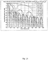
Figure 14 schematically illustrates the Power Spectral Density, PSD, of the BOC(5,2.5) and intermediate signal used for DSB and SBP detector generation.Figure 14 represents the PSD for the BOC(5,2.5) as well as the PSD for left and (resp. right) side lobes, once having being up- (resp. down-) converted to baseband. On the upper part, the PSD is shown for the BOC(5,2.5) signal. On the middle part the PSD is shown for the BOC(5,2.5) after spectral offsetting (to the right) and filtering. Here, the LPF two-sided bandwidth, which is represented with dashed line, is set to four times the chip rate (10MHz) in order to retain as much as possible power from the left spectral contribution of the BOC(5,2.5) PSD (and not starting integrating over the right spectral part). On the lower part the PSD is shown for the BOC(5,2.5) after spectral offsetting (to the left) and filtering. Again, the LPF two-sided bandwidth is also set to four times the chip rate (10MHz). -
Figure 15 schematically illustrates the square root of the absolute value of the Matched Filter, DSB and SBP detectors (BOC(5,2.5)).Figure 15 represents: - the detector characteristics obtained for a matched filter acquisition;
- the detector characteristics obtained for a DSB acquisition; and
- the detector characteristics obtained for a SBP detector acquisition.
- The maximum of the DSB detector equals 0.85 while the maximum of the matched filter detector is 1. This power loss of 1.4 dB is due to the LP filtering applied for generation of the DSB. Similarly, the peak of the SBP detector equals 0.61, when compared to the 0.85 of the DSB, which corresponds to the sqrt(2) scaling factor derived when applying the square root of the the analytical expression for the SBP detector in (Equation 1). Similar curves can be generated for BOC(15,2.5). On
Figure 16 , the two-sided bandwidth of the LP filter is set to eight times the chip rate (or 20MHz), in order to keep as much as possible of the left (resp. right) spectral content of the BOC(15,2.5) without integrating spectral components of the right (resp. left) spectral content. The main outcomes from these curves are that the LP filtering losses, deduced from the main correlation peak amplitude, are smaller than for BOC(15,2.5) as shown infigures 16 and17 , simply because the bandwidth of 20 MHz is larger, and it is possible to keep more side lobes of the equivalent BPSK (at base-band). The number of peaks for the match filter approach is 3 times larger for the BOC(15,2.5) than for the BOC(5,2.5), as a consequence of the higher ratio between sub-carrier and chip rate frequencies. OnFigure 17 , it can be again verified that the ratio between the peak obtained with the DSB and the one obtained with the SBP detector (0.906/0.6445) is equal to sqrt(2), as anticipated from the analytical expressions, (Equation 2). - The following figures represent the distributions in the "H0" (wrong tested hypothesis) and "H1" (right tested hypothesis) case, for the BOC(15,2.5) signal and for a (C/N0) of 25dB-Hz, 30 dB-Hz and 35 dB-Hz.
Figure 18A and 18B schematically illustrate a distribution for the DSB (figure 18A ) and SBP Detector (figure 18B ) in the "H0" and "H1" hypotheses for a BOC(15,2.5) and for 25 dB-Hz.Figure 19A and 19B schematically illustrate a distribution for the DSB (figure 19A ) and SBP Detector (figure 19B ) in the "H0" and "H1" hypotheses for a BOC(15,2.5) and for 30 dB-Hz.Figure 20A and 20B schematically illustrate a Distribution for the DSB (figure 20A ) and SBP Detector (figure 20B ) in the "H0" and "H1" hypotheses for a BOC(15,2.5) and for 35 dB-Hz. Similar curves can be generated for the BOC(5,2.5) case. The following statements can be derived: - for the DSB detector, as expected both "H0" and "H1" distributions are positive, since they are based on a power detector; and
- for the SBP detector, it appears that the "H0" distribution is centred. The "H1" distribution is slightly shifted for a C/N0 of 25 dB-Hz. This shift starts to be more distinct for a C/N0 of 30 dB-Hz. Furthermore, the both "H0" and "H1" distributions can take negative and positive values due to the presence of the noise. Now again the expected or averaged value in the "H1" shall be positive.
- The analysis of the corresponding distributions for the SBP detector enable to propose another improvement based on the usage of the SBP detector. It was highlighted that in the "H1" hypothesis (correct hypothesis), the SBP detector output shall be always positive on average, regardless of the modulated symbol. This characteristic is applied to propose an alternative detection strategy. This one comprises introducing a "third" decision state, as follows:
- if the detector output is positive and is above the detection threshold, "1" ("hit") is allocated;
- if the detector output is positive and is below the detection threshold, "0" ("discard") is allocated; and
- if the detector output is negative then no decision is taken, the SBP detector output is discarded, and another evaluation of the detector output for the same Code and Doppler frequency hypotheses is performed.
- In order to determine how this alternative decision rule can impact the R.O.C curve, the following example is proposed:
For the first detection iteration bringing a SBP detector value, called π1, generated with the first slice samples of Tints: - In the "H0" case:
- ∘ if the detector output is positive and above the detection threshold, then the trial participates to the "PFA", with probability of Prob(π1>Th|π1>0,H0) (=Prob(π1>Th|H0) since Th>0); and
- ∘ if the detector output is negative, no decision is taken and the decision is "reported" to the second detection iteration, applying the same set of Code and Doppler hypotheses. This event has a probability of Prob(π1<0|H0).
- ∘ if the detector output is between 0 and the detection threshold, Th, it is decided that another set of Code and Doppler hypotheses has to be tested. This event has a probability of Prob(0<π1<Th|H0).
- In the "H1" case:
- ∘ if the detector output is positive and higher than the detection threshold, then the corresponding trial participates to the "PD", with a probability of Prob(π1>Th|H1); and
- ∘ if the detector output is negative, no decision is taken and the decision is "reported" to the second detection iteration, applying the same set of Code and Doppler hypotheses. This event has a probability of Prob(π1<0|H1).
- ∘ if the detector output is between 0 and the detection threshold, it is decided that another set of Code and Doppler hypotheses has to be tested, then the corresponding trial participates to the Probability of Missed Detection "PMD", with a probability of Prob(0<π1<Th|H1).
- For the second detection iteration, applying the same set of Code and Doppler hypotheses, and bringing a SBP detector value π2 generated with the second slice samples of Tints:
- In the "H0" case:
- ∘ if the detector output is positive and above the detection threshold, then the trial participates to the "PFA", with a probability of

- ∘ if the detector output is negative, no decision is taken and the decision is "reported" to the third detection iteration, applying the same set of Code and Doppler hypotheses. This event has a probability of

- ∘ if the detector output is between 0 and the detection threshold, it is decided that another set of Code and Doppler hypotheses has to be tested. This event has a probability of Prob(0<π2<Th|H0)× Prob(π1<0|H0).
- ∘ if the detector output is positive and above the detection threshold, then the trial participates to the "PFA", with a probability of
- In the "H1" case:
- ∘ if the detector output is positive and below the detection threshold, then the trial participates to the "PD", with a probability of

- ∘ if the detector output is negative, no decision is taken and the decision is "reported" to the third detection iteration, applying the same set of Code and Doppler hypotheses. This event has a probability of Prob(π2<0|H1)×Prob(π1<0|H1) =(Prob(π<0|H1))2.
- ∘ if the detector output is between 0 and the detection threshold, it is decided that another set of Code and Doppler hypotheses has to be tested, then the corresponding trial participates to the Probability of Missed Detection "PMD", with a probability of Prob(0<π2<Th|H1)×Prob(π1<0|H1).
- ∘ if the detector output is positive and below the detection threshold, then the trial participates to the "PD", with a probability of
- For the third detection iteration, applying the same set of Code and Doppler hypotheses, and bringing a SBP detector value π3 and generated with the third slice samples of Tints:
- In the "H0" case:
- ∘ if the detector output is positive and above the detection threshold, then the trial participates to the "PFA", with probability Prob(π3>Th|H0)×(Prob(π<0|H0))2; and
- ∘ if the detector output is negative, no decision is taken and the decision is "reported" to the fourth detection iteration, applying the same set of Code and Doppler hypotheses. This event has a probability of

- ∘ if the detector output is between 0 and the detection threshold, it is decided that another set of Code and Doppler hypotheses has to be tested. This event has a probability of

- In the "H1" case:
- ∘ if the detector output is positive and below the detection threshold, then the trial participates to the "PD", with probability of

- ∘ if the detector output is negative, no decision is taken and the decision is "reported" to the fourth detection iteration, applying the same set of Code and Doppler hypotheses. This event has a probability of

- ∘ if the detector output is between 0 and the detection threshold, it is decided that another set of Code and Doppler hypotheses has to be tested, then the corresponding trial participates to the Probability of Missed Detection "PMD", with a probability of Prob(0<π3<Th|H1)×Prob(π2<0|H1)×Prob(π1<0|H1)= Prob(0<π<Th|H1)×(Prob(π<0|H1))2.
- ∘ if the detector output is positive and below the detection threshold, then the trial participates to the "PD", with probability of
- This iterative principle can be repeated over successive iterations and estimations of the SBP detector output for the same code and Doppler frequency hypotheses. Therefore, the aggregate PFA and PMD levels can be deduced.


- For a fair comparison of the SBP detector strategy w.r.t. the conventional DSB strategy, it is important to state that by introducing successive tests (for the "negative SBP detector outputs"), one delays the decision, and therefore the Mean-Time-To-Acquire (MTTA). Here a "rough" evaluation of this impact comprises a multiplication with a factor 1.5 corresponding to 50% degradation of the MTTA (since on average, 50% of SBP detector outputs are negative for "H0" case, which mainly impacts the MTTA). As a consequence, this option can be somehow compared to a "double dwell time strategy" applied to a DSB (even if this former one impacts even more the MTTA, since two consecutive decisions are always taken because DSB outputs are always positive). The four probabilities, constitutive of the former modified PFA and PD equations are drawn on the
figure 21. Figure 21 schematically illustrates a model for the SBP detector output in the "H0" and "H1" hypotheses. Based on the distributions generated with the MC simulation it is possible to evaluate these PFA and PD. - One usual and well recognized method to compare detector performances comprises evaluating the Receiver Operational Curves (R.O.C) representing the Probability of Detection (PD) as function of the Probability of False Alarm (PFA) for a varying detection threshold value. To derive these R.O.C. curves both PFA and PD are calculated for a varying detection threshold symbolised with a line designated as Th in
figure 21 . The area above the threshold for the "H0" (resp. "H1") distribution represents the PFA (resp. PD) and is evaluated for each value of the detection threshold. - In the following, the concept of the Sided Band Product detector for BOC-modulated signals is extended to the case of the Generalized-BOC-modulated signals, also called G-BOC, on the one side, and on the other side to the case of a G-BOC with asymmetrical data demodulation, G-BOCAS which can be compared to an Orthogonal Frequency Division Multiplexing (OFDM) signals.
- The Generalized-BOC signal is obtained as the combination of different elementary BOC(Mk,Nk)-modulated signals. The following equation provides the generic expression of a modulated Generalized BOC-Modulated signal obtained by applying an amplitude multiplexing scheme:

- In this expression K represents the number of sub-carrier frequencies. fsc,k represents each sub-carrier frequency. ck(t) represents the spreading sequence constituted of binary symbols, called chips, and whose values depend on time t. Typical spreading sequences are pseudo-random noise sequences such as the Gold codes applied for the GPS CA signals or so-called memory codes, but still periodical codes, such as the Galileo E1-B and codes. The pk(t) is a pulse shape modulating the chips of the spreading sequences which is applied for each sub-carrier frequency and which can be a BPSK(Nk) pulse shape with a chip rate fc,k=N×f0. This pulse shape pk(t) can be different for each elementary BOC(Mk,Nk)-modulated signal. dk(t) is a data symbol applied to each sub-carrier frequency. In case no data symbol is modulated, the corresponding BOC(Mk,Nk)-modulated signal is called a pilot one. P is the aggregate power for multiplexed signal. Furthermore, in the expression of (Equation 57) an amplitude multiplexing scheme has been used for the combination of the K elementary BOC-modulated signals, and a cosine function, cos(2πjfsc,kt), has been applied to multiply the pulse shape pk(t). An equivalent expression for a G-BOC signal can be derived when apply a sinus function, sin(2πfsc,kt), in place of the cosine function, cos(2πjfsc,kt). Finally a complex multiplicative factor αk×e(jϕk) is used on a one side to allot to each elementary BOC(Mk,Nk)-modulated signal a fraction of the aggregate power P using the scaling factor αk and on the other side to set each of the elementary BOC-modulated signal to the In-Phase or Quadrature component using the angle ϕk is the complex exponential argument.
- Alternatively to the amplitude multiplexing scheme, a time multiplexing scheme can also be used. Several mathematical notations can be proposed to express the time multiplexing version of the G-BOC. Here, it is proposed to use the spreading code sequence value to explicitly express the time interval when each elementary BOC(Mk,Nk)-modulated signal is active, while the (K-1) others are not. For this, one denotes by {Tk,u }1≤u≤Uk the ensemble of the time intervals when the elementary BOC(Mk,Nk)-modulated signal is active.
Figure 22 illustrates the case of a time multiplexing comprising K=3 elementary BOC(Mk,Nk)-modulated signals. For this example, the simplified case where all three elementary BOC(Mk,Nk)-modulated signals have the same chip rate is considered (N1=N2=N3), and therefore the chip duration is identical for all three elementary BOC(Mk,Nk)-modulated signals. The underlying spreading sequence which is applied during the coherent integration time, Tint, is shown on the top of thefigure 22 . Then for each elementary BOC(Mk,Nk)-modulated signal, the time intervals {Tk,u }1≤u≤Uk are depicted for k=1, 2 and 3. Furthermore, for each time interval, Tk,u, the corresponding interval centre is denoted Tc k,u. Based on these conventions, the spreading sequence allotted to each elementary BOC(Mk,Nk)-modulated signal is a so-called three-valued sequence, composed on a one side of the binary symbols of the underlying spreading sequence when the elementary BOC(Mk,Nk)-modulated signal is active, and on the other side of a 0 value when the elementary BOC(Mk,Nk)-modulated signal is not activated. This can be described with the following equation:
- Based on the corresponding formalism it is possible present the expression for the G-BOC-modulated signal obtained with the time multiplexing scheme as follows:

- The relative power ratio between the K different elementary BOC(Mk,Nk)-modulated signals is then obtained with the ratio, βk, between the cumulated duration of the time intervals {Tk,u}0≤u≤U over the coherent integration time, Tint and the coherent integration time. This ratio βk can also be related to the amplitude coefficient αk applied for the amplitude multiplexing scheme as follows.

- Where the operator dur(T) evaluates the duration of the interval T.
- As a matter of fact the amplitude coefficient, introduced for the amplitude multiplexing scheme, αk, does not appear in the expression of the time multiplexing scheme since the power ratio between the different elementary BOC(Mk,Nk) signals is expressed with the coefficient βk wich can be related to coefficient αk of the amplitude multiplexing scheme
- In the case of a Generalized BOC-modulated signal using the amplitude multiplexing scheme, the extension of the SBP-Detector comprises multiplying the correlator outputs for the left side lobe with the correlator outputs for the right side lobe for each elementary BOC(Mk,Nk)-modulated signal. The corresponding products are summed up to generate the aggregate detector output (SBP detector) for the Generalized BOC-modulated signal constituted of the K elementary BOC-modulated signals. The expression for the aggregate detector output obtained by applying the former steps is now presented.
- The following equations provides the expression of the correlator output for the left


- In this expression, the term

- The following equation provides the expression of the SBP detector output for the Generalized BOC signals, and obtained with the application of the steps formerly described, and when applying an amplitude multiplexing scheme for the Generalized BOC signals.

- The signification of the other terms and parameters of the (Equation 62) is identical to the (Equation 1) and (Equation 2).
- For information, in the case of a Generalized BOC-modulated signal, using amplitude multiplexing scheme, the extension of the Dual Sided Band-Detector (DSB), called now Multiplexed Band Detector (MSB) becomes:

-
Figure 23 illustrates how the architecture, following conventions offigure 8 , for the proposed acquisition scheme applied for a generalized BOC-modulated signal, when K = 2 (forfigure 8 , K =1). - Another combination of the elementary correlation functions of the elementary BOC(Mk,Nk)-modulated signals can also be proposed in order to yield to a detector which is not sensitive to the ionosphere and hardware group delay. This alternative combination introduces the conjugate operator and can be considered as an extension of the conjugate SBP,


- In the former expressions, it is considered that each signal s1(t) and s2(t) is modulated with a different value d1(t) and d2(t).
- Because the same chip rate, and therefore underlying BPSK(N) primitive pulse shape is applied, the same correlation function Rp(Δτ) appears in all four former equations.
- It is then proposed to combine the former correlation outputs as follows to generate the generalized SBP detector output:

- Where (x) designates the conjugate operator.
- The first product,


- The two pairs of products in the former equation reduce as follow, using the same principle of the SBP applied to a simple BOC modulated signal (squared modulated data is one (dk)2=1 and


- Similarly for the second contribution of the detector output

- At the end, for the proposed example the following expression for this alternative variant of the SBP detector output becomes.

- It can be observed that this detector output is effectively insensitive to the effects of the ionosphere and hardware group delay.
- In the case when s1(t) and s2(t) share the received power in a balanced way (α1 2=α2 2=1/2), then


- Therefore, when compared to a "power detector", such as a MSB detector, the square root of the extended SBP detector has to be taken, yielding to

factor 
Now, the performances of detectors depend generally on the relative ratio between the power of the signal to be detected, acquired and the power for the noise contribution to the detector. - Therefore, the individual noise contribution for each of the four complex correlation outputs needs also to be accounted, re-using the notations of (Equation 34), (Equation 35), (Equation 36) and (Equation 37):

- It must be underlined that the four former complex correlations, to be considered as stochastic variables, are Gaussians, centred and also independent between each other since resulting from a filtering of the different spectral contents of the occupation of the G-BOC signal as presented on
Figure 24 . -
Figure 24 schematically illustrates the independency of the four noise contributions involved in the calculation of the generalized SBP detector applicable to a Generalized BOC modulated signal with K=2. It can effectively be verified that the spectral occupation of the four aforementioned noise components are disjoint and enables to better justify their independency as stochastic variable. - Taken again the expression of the extended expression for the SBD of (Equation 65), and considering a wrong hypothesis in code or Doppler ("H0" case), the SBP expression can be simplified by replacing each correlation contribution with the former


- Because the four noise contributions are independent pairwise, this property will enable to also strongly reduce the mean and variance of the SBP detector output which is desired.
- The average of the extended SBP detector output is given by the following equation.

- Due to the centered stochastic terms for the noise contribution, the average of the extended SBP detector is therefore null. This is an important advantage w.r.t. the conventional MSB detector whose average depends on the variance of the individual stochastic terms. This additional term could effectively yield to an increase in the PFA for the "H0" hypothesis. This is not the case for the extended SBP detector applied to generalized BOC modulated signals.
- The variance of the extended SBP detector output is given by the following equation.

- The first term can be rewritten as:

- Because the stochastic terms (


- With ρij = E{ni × nj} and V represents the total number of combinations for the multiplications of four terms of the form ρij. It is important to note that each index i, j, k, I, m, n, o and p only appears once for each contribution [ρi,j×ρk,l×ρm,n×ρo,p].
- The application of the former theorem to (Equation 74) enables to identify one term which is not zero, over the V=105 individual products of the form [ρi,j×ρk,l×ρm,n×ρo,p]. This term is

- For the same reason of independency between terms ni and nj} for i≠j, and their zero mean,

- As a conclusion the variance can be reduced to the following

- These calculations highlight the benefit of the alternative definition with

factor 
- It must be noted that the former derivations of the variance in the "H0" case, can be also applied in the "H1" case, and show again that compared to the conventional power detectors, such as the MSB the contribution of the stochastic contribution onto the extended SBP detector is also reduced due to the combined effect of independency between terms ni and nj} for i≠j, and their mean value.
- It must also be remarked that in (Equation 65), a single product can also be considered to define the acquisition detector, as shown on the following equation, and shall not impact the ratio between the signal and noise power of the extended detector SBP detector, and therefore the detection performances.

- The former equation can also be expressed as

- This equation enables to understand that the alternative detector definition of (Equation 65) applied in the case of K ≥2 sub-carriers is a generalization of the detector obtained with the complex conjugate multiplication when K =1 of (Equation 28).
- The former derivations and benefit justifications for the introduction of the alternative definition of an SBP detector to be applied to a Generalized BOC modulated signal, in the case of K=2 can be generalized for any K as follows:

- In the
former equation 

- Here again it is possible to add non-coherently different SBP detectors using the computed on successive coherent integration times yielding:

- It has to be noted that the following variants of the equation (Equation 79) can be proposed to define the extended SBP detector:


- In (Equation 81) the normalization with the
combination number 
- In the case of a Generalized BOC-modulated signal using the time multiplexing scheme, the definition of the SBP-Detector comprises multiplying the correlator outputs for the left side lobe with the correlator outputs for the right side lobe for each elementary BOC(Mk,Nk)-modulated signal. The corresponding products are summed up to generate the aggregate detector output (SBP detector) for the Generalized BOC-modulated signal constituted of the K elementary BOC-modulated signals. The expression for the aggregate detector output is presented.
- The (Equation 83) provides the expression of the correlator output for the left


- For the derivation of (Equation 83) it was necessary to take into account the centre of the corresponding time intervals, Tc k,u, with the
exponential 
- Furthermore, in the derivation of the former equation (Equation 83), the coherent integration time used to compute the K partials correlations corresponding to the K elementary BOC(Mk,Nk)-modulated signals equals Tint as shown on
Figure 22 , and therefore each correlation is weighted with the coefficient βk introduced in (Equation 60). - The following equation provides the expression of the SBP detector output obtained with the application of the steps formerly described, and when applying a time multiplexing scheme for the Generalized BOC signals.

- In a similar manner to the definition of the alternative definition of SBP detector output introducing the conjugate operation and applied for a generalized BOC modulated signal with an amplitude modulation scheme, it is also possible to propose an alternative definition for a SBP detector output introducing the conjugate operation for a generalized BOC modulated signal with a time modulation scheme as shown below

- Again, other variants of the proposed SBP definition similar to (Equation 81) and (Equation 82) can be also introduced in the case of a time multiplexing scheme.
- Here again it is possible to improve the acquisition performances by adding non-coherently different SBP detectors using the computed on successive coherent integration times yielding:

- A further extension of the Side Band Product detector covers the case of a G-BOC for which the lower and upper sideband signal do not contain obligatory the same symbol or data for each of the elementary BOC(Mk,Nk)-modulated signals. This type of G-BOC is called G-BOC signal with asymmetrical data modulation and will be called G-BOCAS signal in the present disclosure. Hence instead of being composed with K sub-carriers this variant of the G-BOC is composed of I carrier frequencies, with I=2K.
-
Figure 25 schematically illustrates the generation of a G-BOCAS signal. - The following equation provides the generic expression for a G-BOC signal with asymmetrical data modulation at baseband:

- In this expression, I represents the number of carrier frequencies. fi represents each carrier frequency. pi(t) is a pulse shape which modulates each carrier frequency. di(t) is a data or symbol applied to each carrier frequency. In the present disclosure, the term data is used generically and can either correspond to symbols, when a coding scheme such as a Convolutional or a Turbo encoder is used to transform data into symbols, or to data when no encoder is applied. The complex factor αi×ej(ϕi) has the same signification and purpose as for the G-BOC-modulated signal.
- Due to the usage of the exponential term, exp(2πfit) in (Equation 87) applicable for the G-BOC with asymmetrical data modulation case, instead of the cosine term, cos(2πf sc, kt), as proposed in the equation (Equation 57) for the G-BOC case, and illustrated on
Figure 25 , it is possible to modulate a different data on each of the I individual carrier frequencies, fi. In contrast, in the case of the G-BOC the same data is modulated on both carriers +fsc,k and -fsc,k, decomposing the cosine term cos(2πfsc,kt) as (exp(2πjfit) + exp(-2πjfit)) / 2. The same justification would hold if a sinus function sin(2πfsc,kt) is applied in place of the cosine function in (Equation 57). It has to be noted that expression (Equation 87) can also represent the general class of the Orthogonal Frequency Division Multiplexing (OFDM) signals. The equation (Equation 87) is again an extension of the G-BOC signal introduced in the frame of the acquisition of such signals. - Usually, a practical implementation for the generation (i.e. modulation of the I data di(t)) comprises having, the I carrier frequencies {fi}1≤i≤I uniformly spaced

- Where fu is a reference frequency used for the generation of the I elementary frequencies.
- Furthermore, if I takes the form of I=2V it is possible to generate the G-BOCAS signal sGBOCAS (tk ) at epoch tk, and modulate the I data di(tk) by using a Discrete Fourier Transform (DFT). Similarly from the G-BOCAS signal sGBOCAS (tk ), it is possible to retrieve or demodulate the I data using an Inverse Discrete Fourier Transform. Hence, at each time epoch tk the I data can be modulated (resp. demodulated) simultaneously when using a DFT (resp. IDFT).
- In order to apply to the G-BOCAS signals the principle of the Sided Band Product, firstly introduced to the cases of BOC and Generalized BOC-modulated signals some constraints need to be imposed to the G-BOCAS signal structure, and especially to the data modulation.
-
Figure 26 schematically illustrates a Time-Frequency Domain Pattern of modulated data of a G-BOCAS signal.Figure 26 shows the case for I =8 (=23 and V=3) carriers. This representation considers that the signal is sampled at a uniform frequency, fs, equal to the inverse of sampling interval, Ts. Two sampling epochs tk and tk+1 are therefore spaced by Ts. At each epoch tk, 8 data are modulated and represented with a white circle for a binary value of 0 and a black circle for the binary value of 1. Here the pulse shape pi(tk) and the corresponding spectral occupancy are not represented for sake of clarity. In order to adapt the present invention for such a G-BOCAS signal it is necessary to ensure "symmetry" of the data modulated on each of the I carriers with respect to a central frequency, usually the carrier frequency. The corresponding modified Time-Frequency Domain Pattern of the G-BOCAS signal is represented onfigure 27 . -
Figure 27 schematically illustrates a Time-Frequency Domain Pattern of Modulated Data of a G-BOCAS signal according to an embodiment of the present invention.Figure 27 shows an arrangement of data for the application of the SBP Detector during acquisition. The arrangement of data in the Time-Frequency Domain Pattern is symmetrical to the carrier frequency considered as central frequency. G-BOCAS processing is usually based on a Discrete Fourier Transform (DFT). To recover the data or symbol, the DFT of the G-BOCAS signal is calculated (DFT(23) in the example offigure 27 ), and the values of the I Fourier components, DFT(sGBOCAS (tk ),i), provide the values for the I data. For acquisition, it is also possible to apply the DFT operation. Using the analogy to the DSB acquisition scheme applicable for the BOC signal, the sum of squared absolute values of the I Fourier components is calculated, yielding to a Multi-Side Band (MSB) acquisition detector:
- As for the DSB acquisition approach, the square operation is necessary to be immune against the data or symbol signs.
- In order to generate a detector which shall not suffer from the effect of the data or symbol signs, it is proposed to form the following alternative detector, equivalent to the SBP detector for BOC signals:

- In this expression, each DFT(sGBOCAS (tk ),i) component is multiplied with its symmetrical component DFT(sGBOCAS (tk ),I-i+1) with respect to the central frequency, i.e. carrier frequency.
- Here again it is possible to improve the acquisition performances by adding non-coherently different detectors computed on successive coherent integration times yielding:

- Due to the independence of the noise contribution in each Fourier component DFT(sGBOCAS (tk ),i), each of the I/2 products in the former expression is centred, and therefore the sum of the 1/2 products too. Hence the distribution for the

- If the symmetry between pairs of data modulated on different carriers is not ensured at each epoch tk, but at two different epochs tk and tk+l, it is still possible to multiply the corresponding components DFT(sGBOCAS (tk ),i) and DFT(sGBOCAS (tk+l ),I-i+1), but the phase delay between the two identical data transmitted on symmetrical frequency needs to be compensated. The expression of the modified detector output accounting for data which are time-differed within the pairs is following

- Here, the correction factor ϕ(fi(tk),δti(tk)) which enables to compensate for the differed time between identical data within each pair of components is given by the following expression:

- Here δti (tk ) represents the time delay between two identical data transmitted on symmetrical frequencies which depend on the component index i and epoch tk as indicated on
Figure 28 . - The main difference w.r.t. the case when the data pattern has been symmetrized is that each data corresponding to a frequency i and epoch tk has to be involved only once in expression (Equation 92).
- Here again it is possible to improve the acquisition performances by adding non-coherently different detectors computed on successive coherent integration times yielding:

-
Figure 28 schematically illustrates a Time-Frequency Domain Pattern of Modulated data of a G-BOCAS signal according to an embodiment of the present invention.Figure 28 shows an arrangement of data for epoch tk for the application of the SBP detector for the acquisition of a G-BOCAS signals when identical data belonging to two symmetrical components are differed. For each pair of components (i=1, 2, 3 and 4), the time offset δti(tk) is represented for each pair of components fi. The data which are not part of the calculation of the detector output
Claims (14)
- A method for signal acquisition of a Generalized Binary Offset Carrier, G-BOC, modulated signal comprising K elementary BOC(Mk,Nk)-modulated signals, the method comprising:retrieving, for each of the K elementary BOC(Mk,Nk)-modulated signals, a lower sideband signal and an upper sideband signal by respectively up-converting and down-converting the respective elementary BOC(Mk,Nk)-modulated signal under use of a sub-carrier frequency fsc,k corresponding to the respective elementary BOC(Mk,Nk)-modulated signal and by respectively low-pass filtering the respective up-converted and down-converted elementary BOC(Mk,Nk)-modulated signal;respectively correlating a replica modulated with the primitive pulse shape involved in the generation of the BOC(Mk,Nk)-modulated signal such as a binary phase shift keying, BPSK, pulse shape with the retrieved lower and upper sideband signals, wherein the replica has a chip rate and a spreading sequence according to the respective elementary BOC(Mk,Nk)-modulated signal and the replica is generated on the basis of a code delay hypothesis and a Doppler frequency hypothesis;applying either step (a) or step (b), where step (a) comprises:multiplying the respective correlation results with each other by complex or complex conjugate multiplication;generating a first detector output by adding the corresponding K complex or K complex conjugate multiplications and/or generating a second detector output by adding NNC successive detector outputs, each being the sum of the K complex or K complex conjugate multiplications; and step (b) comprises:
for pairs of distinct elements in a group of K, for each identified pair of signals si and sj, multiplying the correlating results derived from the retrieved lower sideband signal of si, Rsi left(t) with the correlation result derived from the upper sideband signal si, Rsi right(t), by complex multiplication and multiplying the correlating result derived from the retrieved lower sideband signal of sj, Rsj left(t), with the correlation result derived from the upper sideband signal sj, Rsj right(t), by complex multiplication; when K=2, a first detector output is generated as

- The method according to claim 1, wherein the detection threshold is set to a probability of false alarm or a probability of missed detection.
- The method according to any one of the foregoing claims, wherein correlating comprises a coherent integration, wherein the coherent integration is performed over a time duration being equal or lower than a symbol duration, when symbols or data are included in data modulated on the G-BOC-modulated signal.
- The method according to claim 3, wherein the time duration for the coherent integration time is based on a dynamic of a link between a transmitter and a receiver.
- The method according to any one of the foregoing claims, wherein a hardware group delay and/or a carrier delay is estimated and included in the complex or complex conjugate multiplication, wherein the carrier delay is based on an ionospheric effect.
- The method according to any one of the foregoing claims, wherein only the real part of the detector output indicates detection.
- The method according to claim 6, wherein only a positive detector output is compared to the detection threshold and a negative detector output is discarded or ignored.
- The method according to any one of the foregoing claims, wherein the G-BOC-modulated signal comprises K sub-carriers, wherein K is an integer number, wherein the K sub-carriers are multiplexed either with an amplitude or a time multiplexing scheme, wherein each of the K sub-carriers is modulated with data or not.
- The method according to claim 8, wherein, in particular when the G-BOC-modulated signal is modulated with symbols, a number of symbols is I=2×K corresponding to the number of carriers I, and a time-frequency domain pattern of the I symbols is symmetrical or is not symmetrical to a central carrier of the G-BOC-modulated signal.
- The method according to claims 8 or 9, wherein the I symbols correspond to I Fourier components forming a symmetrical time-frequency pattern and are determined by a Discrete or Fast Fourier Transform, and wherein the step of combining comprises complex multiplication of the Fourier components.
- The method according to claims 8 or 9, wherein the I symbols correspond to I Fourier components forming an asymmetrical time-frequency pattern determined by a Discrete or Fast Fourier Transform, and wherein the step of combining comprises:selecting pairs of the I symbols over time such that their values is identical and their frequencies are symmetrical to the central carrier of the G-BOC-modulated signal,multiplying the selected pairs with a correction factor accounting for the time offset between each of the selected pairs, andcomplex multiplying the corrected I Fourier components.
- A computer program which when carried out on a processor of a device for signal acquisition of a Generalized Binary Offset Carrier, G-BOC, causes the processor to carry out the method of any one of the foregoing claims.
- A storage device storing a computer program according to claim 12.
- A device for signal acquisition of a Generalized Binary Offset Carrier, G-BOC, modulated signal comprising K elementary BOC(Mk,Nk)-modulated signals, comprising:an up-converter and a low-pass filter adapted to retrieve, for each of the K elementary BOC(Mk,Nk)-modulated signals, a lower sideband signal by up-converting the respective elementary BOC(Mk,Nk)-modulated signal under use of a sub-carrier frequency fsc,k corresponding to the respective elementary BOC(Mk,Nk)-modulated signal and by low-pass filtering the respective up-converted elementary BOC(Mk,Nk)-modulated signal;a down-converter and a low-pass filter adapted to retrieve, for each of the K elementary BOC(Mk,Nk)-modulated signals an upper sideband signal by down-converting the respective elementary BOC(Mk,Nk)-modulated signal under use of the sub-carrier frequency fsc,k corresponding to the respective elementary BOC(Mk,Nk)-modulated signal and by low-pass filtering the respective down-converted elementary BOC(Mk,Nk)-modulated signal;a correlating unit adapted to respectively correlate a replica modulated with the primitive pulse shape involved in the generation of the BOC(Mk,Nk)-modulated signal such as a binary phase shift keying, BPSK, pulse shape with the retrieved lower and upper sideband signals, wherein the replica has a chip rate and a spreading sequence according to the respective elementary BOC(Mk,Nk)-modulated signal and the replica is generated on the basis of a code delay hypothesis and a Doppler frequency hypothesis;a detecting unit adapted to either (a):
multiply the respective correlation results with each other by complex or complex conjugate multiplication and to generate a detector output by adding the corresponding K complex or K complex conjugate multiplications and/or by adding NNC successive detector outputs, each being the sum of the K complex or K complex conjugate multiplications or (b):
for pairs of distinct elements in a group of K, for each identified pair of signals si and sj, multiplying the correlating results derived from the retrieved lower sideband signal of si, Rsi left(t) with the correlation result derived from the upper sideband signal si, Rsi right(t), by complex multiplication and multiplying the correlating results derived from the retrieved lower sideband signal of sj, Rsj left(t), with the correlation result derived from the upper sideband signal sj, Rsj right(t), by complex multiplication; when K=2, a detector output is generated as

an acquisition unit adapted to acquire the G-BOC-modulated signal corresponding to the code delay hypothesis and the Doppler frequency hypothesis, when the detector output being compared to a detection threshold indicates detection.
Priority Applications (2)
| Application Number | Priority Date | Filing Date | Title |
|---|---|---|---|
| EP17189747.3A EP3454090B1 (en) | 2017-09-07 | 2017-09-07 | A method and device for signal acquisition of a generalized boc-modulated signal |
| PCT/EP2018/073393 WO2019048341A1 (en) | 2017-09-07 | 2018-08-30 | A method and device for signal acquisition of a generalized boc-modulated signal |
Applications Claiming Priority (1)
| Application Number | Priority Date | Filing Date | Title |
|---|---|---|---|
| EP17189747.3A EP3454090B1 (en) | 2017-09-07 | 2017-09-07 | A method and device for signal acquisition of a generalized boc-modulated signal |
Publications (2)
| Publication Number | Publication Date |
|---|---|
| EP3454090A1 EP3454090A1 (en) | 2019-03-13 |
| EP3454090B1 true EP3454090B1 (en) | 2020-11-04 |
Family
ID=59846393
Family Applications (1)
| Application Number | Title | Priority Date | Filing Date |
|---|---|---|---|
| EP17189747.3A Active EP3454090B1 (en) | 2017-09-07 | 2017-09-07 | A method and device for signal acquisition of a generalized boc-modulated signal |
Country Status (2)
| Country | Link |
|---|---|
| EP (1) | EP3454090B1 (en) |
| WO (1) | WO2019048341A1 (en) |
Families Citing this family (8)
| Publication number | Priority date | Publication date | Assignee | Title |
|---|---|---|---|---|
| EP3905536A1 (en) * | 2020-04-28 | 2021-11-03 | Airbus Defence and Space GmbH | Noise distribution shaping for cdma signals |
| CN111884700B (en) * | 2020-06-03 | 2021-11-23 | 中国人民解放军军事科学院国防科技创新研究院 | Pilot positioning message processing device and method based on low-earth orbit satellite |
| CN112578412A (en) * | 2020-11-24 | 2021-03-30 | 中国电子科技集团公司第二十研究所 | Capturing method compatible with B1C signal and B2a signal |
| CN113721272A (en) * | 2021-08-31 | 2021-11-30 | 广东工业大学 | Method for capturing Beidou satellite navigation B1C signal and related device thereof |
| WO2023166227A1 (en) | 2022-03-04 | 2023-09-07 | The European Union, Represented By The European Commission | Method for acquisition of a radio signal component of a plurality of radio signal components, a related radio navigation system, a related radio transmitter and a related radio receiver. |
| CN114690212B (en) * | 2022-03-18 | 2024-05-14 | 中国科学院国家空间科学中心 | Method and system for performing interference early warning by using DDM data quality monitoring |
| CN115047501B (en) * | 2022-08-15 | 2022-11-08 | 长沙学院 | Satellite navigation authorization signal estimation method suitable for BOC modulation |
| CN116094890B (en) * | 2022-11-21 | 2023-06-30 | 重庆大学 | Communication signal transmission method based on integrated signal |
Family Cites Families (2)
| Publication number | Priority date | Publication date | Assignee | Title |
|---|---|---|---|---|
| US7224721B2 (en) * | 2002-10-11 | 2007-05-29 | The Mitre Corporation | System for direct acquisition of received signals |
| CN104375151B (en) * | 2014-09-19 | 2016-10-19 | 清华大学 | Navigation signal receiver and method of reseptance |
-
2017
- 2017-09-07 EP EP17189747.3A patent/EP3454090B1/en active Active
-
2018
- 2018-08-30 WO PCT/EP2018/073393 patent/WO2019048341A1/en active Application Filing
Non-Patent Citations (1)
| Title |
|---|
| None * |
Also Published As
| Publication number | Publication date |
|---|---|
| EP3454090A1 (en) | 2019-03-13 |
| WO2019048341A1 (en) | 2019-03-14 |
Similar Documents
| Publication | Publication Date | Title |
|---|---|---|
| EP3454090B1 (en) | A method and device for signal acquisition of a generalized boc-modulated signal | |
| US6282231B1 (en) | Strong signal cancellation to enhance processing of weak spread spectrum signal | |
| EP2701323B1 (en) | Generating and processing of CDMA signals | |
| US6236354B1 (en) | Reducing satellite signal interference in a global positioning system receiver | |
| US8237611B2 (en) | Method for processing combined navigation signals | |
| Yang et al. | Acquisition of the GPS L5 signal using coherent combining of I5 and Q5 | |
| US8830123B2 (en) | Satellite navigation system for optimal time to first fix using code and carrier diversity | |
| US11121738B2 (en) | Radio receiver | |
| US20070211791A1 (en) | Coherent processing using composite codes | |
| EP3109673A1 (en) | Gnss receiver with an improved capability to resolve sub-carrier tracking ambiguities | |
| Shanmugam | New enhanced sensitivity detection techniques for GPS L 1 C/A and modernized signal acquisition | |
| Deshpande | Study of interference effects on GPS signal acquisition | |
| US11579309B2 (en) | Global Navigation Satellite System (GNSS) multipath mitigation | |
| US10094929B2 (en) | Method for carrier-to-noise ratio estimation in GNSS receivers | |
| O'Driscoll et al. | Band-limiting and Dispersive Effects on High Order BOC Signals | |
| CN110501728B (en) | Frequency discrimination method and device for time hopping signal of positioning base station | |
| Borio | Double phase estimator: new results | |
| Han et al. | Investigation on Figures-of-Merit of Signal Performance for Next Generation RNSS Signal Design | |
| Fernández et al. | Galileo Receiver performance under GPS interference and multipath with the GRANADA Software Receiver | |
| Borio et al. | Quality monitoring of BOC signals through codeless techniques | |
| Borio et al. | Bicomplex Kalman Filter Tracking for GNSS Meta-Signals | |
| Petovello et al. | Impact of notch filtering on tracking loops for GNSS applications | |
| Channarayapatna Shivaramaiah | Enhanced receiver techniques for Galileo E5 AltBOC signal processing |
Legal Events
| Date | Code | Title | Description |
|---|---|---|---|
| PUAI | Public reference made under article 153(3) epc to a published international application that has entered the european phase |
Free format text: ORIGINAL CODE: 0009012 |
|
| STAA | Information on the status of an ep patent application or granted ep patent |
Free format text: STATUS: THE APPLICATION HAS BEEN PUBLISHED |
|
| AK | Designated contracting states |
Kind code of ref document: A1 Designated state(s): AL AT BE BG CH CY CZ DE DK EE ES FI FR GB GR HR HU IE IS IT LI LT LU LV MC MK MT NL NO PL PT RO RS SE SI SK SM TR |
|
| AX | Request for extension of the european patent |
Extension state: BA ME |
|
| STAA | Information on the status of an ep patent application or granted ep patent |
Free format text: STATUS: REQUEST FOR EXAMINATION WAS MADE |
|
| 17P | Request for examination filed |
Effective date: 20190528 |
|
| RBV | Designated contracting states (corrected) |
Designated state(s): AL AT BE BG CH CY CZ DE DK EE ES FI FR GB GR HR HU IE IS IT LI LT LU LV MC MK MT NL NO PL PT RO RS SE SI SK SM TR |
|
| STAA | Information on the status of an ep patent application or granted ep patent |
Free format text: STATUS: EXAMINATION IS IN PROGRESS |
|
| 17Q | First examination report despatched |
Effective date: 20190923 |
|
| GRAP | Despatch of communication of intention to grant a patent |
Free format text: ORIGINAL CODE: EPIDOSNIGR1 |
|
| STAA | Information on the status of an ep patent application or granted ep patent |
Free format text: STATUS: GRANT OF PATENT IS INTENDED |
|
| INTG | Intention to grant announced |
Effective date: 20200520 |
|
| GRAS | Grant fee paid |
Free format text: ORIGINAL CODE: EPIDOSNIGR3 |
|
| GRAA | (expected) grant |
Free format text: ORIGINAL CODE: 0009210 |
|
| STAA | Information on the status of an ep patent application or granted ep patent |
Free format text: STATUS: THE PATENT HAS BEEN GRANTED |
|
| AK | Designated contracting states |
Kind code of ref document: B1 Designated state(s): AL AT BE BG CH CY CZ DE DK EE ES FI FR GB GR HR HU IE IS IT LI LT LU LV MC MK MT NL NO PL PT RO RS SE SI SK SM TR |
|
| REG | Reference to a national code |
Ref country code: GB Ref legal event code: FG4D |
|
| REG | Reference to a national code |
Ref country code: CH Ref legal event code: EP |
|
| REG | Reference to a national code |
Ref country code: AT Ref legal event code: REF Ref document number: 1331533 Country of ref document: AT Kind code of ref document: T Effective date: 20201115 |
|
| REG | Reference to a national code |
Ref country code: IE Ref legal event code: FG4D |
|
| REG | Reference to a national code |
Ref country code: DE Ref legal event code: R096 Ref document number: 602017026689 Country of ref document: DE |
|
| REG | Reference to a national code |
Ref country code: NL Ref legal event code: MP Effective date: 20201104 |
|
| REG | Reference to a national code |
Ref country code: AT Ref legal event code: MK05 Ref document number: 1331533 Country of ref document: AT Kind code of ref document: T Effective date: 20201104 |
|
| PG25 | Lapsed in a contracting state [announced via postgrant information from national office to epo] |
Ref country code: NO Free format text: LAPSE BECAUSE OF FAILURE TO SUBMIT A TRANSLATION OF THE DESCRIPTION OR TO PAY THE FEE WITHIN THE PRESCRIBED TIME-LIMIT Effective date: 20210204 Ref country code: PT Free format text: LAPSE BECAUSE OF FAILURE TO SUBMIT A TRANSLATION OF THE DESCRIPTION OR TO PAY THE FEE WITHIN THE PRESCRIBED TIME-LIMIT Effective date: 20210304 Ref country code: RS Free format text: LAPSE BECAUSE OF FAILURE TO SUBMIT A TRANSLATION OF THE DESCRIPTION OR TO PAY THE FEE WITHIN THE PRESCRIBED TIME-LIMIT Effective date: 20201104 Ref country code: GR Free format text: LAPSE BECAUSE OF FAILURE TO SUBMIT A TRANSLATION OF THE DESCRIPTION OR TO PAY THE FEE WITHIN THE PRESCRIBED TIME-LIMIT Effective date: 20210205 Ref country code: FI Free format text: LAPSE BECAUSE OF FAILURE TO SUBMIT A TRANSLATION OF THE DESCRIPTION OR TO PAY THE FEE WITHIN THE PRESCRIBED TIME-LIMIT Effective date: 20201104 |
|
| PG25 | Lapsed in a contracting state [announced via postgrant information from national office to epo] |
Ref country code: SE Free format text: LAPSE BECAUSE OF FAILURE TO SUBMIT A TRANSLATION OF THE DESCRIPTION OR TO PAY THE FEE WITHIN THE PRESCRIBED TIME-LIMIT Effective date: 20201104 Ref country code: BG Free format text: LAPSE BECAUSE OF FAILURE TO SUBMIT A TRANSLATION OF THE DESCRIPTION OR TO PAY THE FEE WITHIN THE PRESCRIBED TIME-LIMIT Effective date: 20210204 Ref country code: IS Free format text: LAPSE BECAUSE OF FAILURE TO SUBMIT A TRANSLATION OF THE DESCRIPTION OR TO PAY THE FEE WITHIN THE PRESCRIBED TIME-LIMIT Effective date: 20210304 Ref country code: LV Free format text: LAPSE BECAUSE OF FAILURE TO SUBMIT A TRANSLATION OF THE DESCRIPTION OR TO PAY THE FEE WITHIN THE PRESCRIBED TIME-LIMIT Effective date: 20201104 Ref country code: PL Free format text: LAPSE BECAUSE OF FAILURE TO SUBMIT A TRANSLATION OF THE DESCRIPTION OR TO PAY THE FEE WITHIN THE PRESCRIBED TIME-LIMIT Effective date: 20201104 Ref country code: AT Free format text: LAPSE BECAUSE OF FAILURE TO SUBMIT A TRANSLATION OF THE DESCRIPTION OR TO PAY THE FEE WITHIN THE PRESCRIBED TIME-LIMIT Effective date: 20201104 Ref country code: ES Free format text: LAPSE BECAUSE OF FAILURE TO SUBMIT A TRANSLATION OF THE DESCRIPTION OR TO PAY THE FEE WITHIN THE PRESCRIBED TIME-LIMIT Effective date: 20201104 |
|
| REG | Reference to a national code |
Ref country code: LT Ref legal event code: MG9D |
|
| PG25 | Lapsed in a contracting state [announced via postgrant information from national office to epo] |
Ref country code: HR Free format text: LAPSE BECAUSE OF FAILURE TO SUBMIT A TRANSLATION OF THE DESCRIPTION OR TO PAY THE FEE WITHIN THE PRESCRIBED TIME-LIMIT Effective date: 20201104 |
|
| PG25 | Lapsed in a contracting state [announced via postgrant information from national office to epo] |
Ref country code: RO Free format text: LAPSE BECAUSE OF FAILURE TO SUBMIT A TRANSLATION OF THE DESCRIPTION OR TO PAY THE FEE WITHIN THE PRESCRIBED TIME-LIMIT Effective date: 20201104 Ref country code: SK Free format text: LAPSE BECAUSE OF FAILURE TO SUBMIT A TRANSLATION OF THE DESCRIPTION OR TO PAY THE FEE WITHIN THE PRESCRIBED TIME-LIMIT Effective date: 20201104 Ref country code: SM Free format text: LAPSE BECAUSE OF FAILURE TO SUBMIT A TRANSLATION OF THE DESCRIPTION OR TO PAY THE FEE WITHIN THE PRESCRIBED TIME-LIMIT Effective date: 20201104 Ref country code: LT Free format text: LAPSE BECAUSE OF FAILURE TO SUBMIT A TRANSLATION OF THE DESCRIPTION OR TO PAY THE FEE WITHIN THE PRESCRIBED TIME-LIMIT Effective date: 20201104 Ref country code: CZ Free format text: LAPSE BECAUSE OF FAILURE TO SUBMIT A TRANSLATION OF THE DESCRIPTION OR TO PAY THE FEE WITHIN THE PRESCRIBED TIME-LIMIT Effective date: 20201104 Ref country code: EE Free format text: LAPSE BECAUSE OF FAILURE TO SUBMIT A TRANSLATION OF THE DESCRIPTION OR TO PAY THE FEE WITHIN THE PRESCRIBED TIME-LIMIT Effective date: 20201104 |
|
| REG | Reference to a national code |
Ref country code: DE Ref legal event code: R097 Ref document number: 602017026689 Country of ref document: DE |
|
| PG25 | Lapsed in a contracting state [announced via postgrant information from national office to epo] |
Ref country code: DK Free format text: LAPSE BECAUSE OF FAILURE TO SUBMIT A TRANSLATION OF THE DESCRIPTION OR TO PAY THE FEE WITHIN THE PRESCRIBED TIME-LIMIT Effective date: 20201104 |
|
| PLBE | No opposition filed within time limit |
Free format text: ORIGINAL CODE: 0009261 |
|
| STAA | Information on the status of an ep patent application or granted ep patent |
Free format text: STATUS: NO OPPOSITION FILED WITHIN TIME LIMIT |
|
| 26N | No opposition filed |
Effective date: 20210805 |
|
| PG25 | Lapsed in a contracting state [announced via postgrant information from national office to epo] |
Ref country code: NL Free format text: LAPSE BECAUSE OF FAILURE TO SUBMIT A TRANSLATION OF THE DESCRIPTION OR TO PAY THE FEE WITHIN THE PRESCRIBED TIME-LIMIT Effective date: 20201104 Ref country code: AL Free format text: LAPSE BECAUSE OF FAILURE TO SUBMIT A TRANSLATION OF THE DESCRIPTION OR TO PAY THE FEE WITHIN THE PRESCRIBED TIME-LIMIT Effective date: 20201104 Ref country code: IT Free format text: LAPSE BECAUSE OF FAILURE TO SUBMIT A TRANSLATION OF THE DESCRIPTION OR TO PAY THE FEE WITHIN THE PRESCRIBED TIME-LIMIT Effective date: 20201104 |
|
| PG25 | Lapsed in a contracting state [announced via postgrant information from national office to epo] |
Ref country code: SI Free format text: LAPSE BECAUSE OF FAILURE TO SUBMIT A TRANSLATION OF THE DESCRIPTION OR TO PAY THE FEE WITHIN THE PRESCRIBED TIME-LIMIT Effective date: 20201104 |
|
| REG | Reference to a national code |
Ref country code: CH Ref legal event code: PL |
|
| REG | Reference to a national code |
Ref country code: BE Ref legal event code: MM Effective date: 20210930 |
|
| PG25 | Lapsed in a contracting state [announced via postgrant information from national office to epo] |
Ref country code: IS Free format text: LAPSE BECAUSE OF FAILURE TO SUBMIT A TRANSLATION OF THE DESCRIPTION OR TO PAY THE FEE WITHIN THE PRESCRIBED TIME-LIMIT Effective date: 20210304 Ref country code: MC Free format text: LAPSE BECAUSE OF FAILURE TO SUBMIT A TRANSLATION OF THE DESCRIPTION OR TO PAY THE FEE WITHIN THE PRESCRIBED TIME-LIMIT Effective date: 20201104 |
|
| PG25 | Lapsed in a contracting state [announced via postgrant information from national office to epo] |
Ref country code: LU Free format text: LAPSE BECAUSE OF NON-PAYMENT OF DUE FEES Effective date: 20210907 Ref country code: IE Free format text: LAPSE BECAUSE OF NON-PAYMENT OF DUE FEES Effective date: 20210907 Ref country code: BE Free format text: LAPSE BECAUSE OF NON-PAYMENT OF DUE FEES Effective date: 20210930 |
|
| PG25 | Lapsed in a contracting state [announced via postgrant information from national office to epo] |
Ref country code: LI Free format text: LAPSE BECAUSE OF NON-PAYMENT OF DUE FEES Effective date: 20210930 Ref country code: CH Free format text: LAPSE BECAUSE OF NON-PAYMENT OF DUE FEES Effective date: 20210930 |
|
| PG25 | Lapsed in a contracting state [announced via postgrant information from national office to epo] |
Ref country code: CY Free format text: LAPSE BECAUSE OF FAILURE TO SUBMIT A TRANSLATION OF THE DESCRIPTION OR TO PAY THE FEE WITHIN THE PRESCRIBED TIME-LIMIT Effective date: 20201104 |
|
| PG25 | Lapsed in a contracting state [announced via postgrant information from national office to epo] |
Ref country code: HU Free format text: LAPSE BECAUSE OF FAILURE TO SUBMIT A TRANSLATION OF THE DESCRIPTION OR TO PAY THE FEE WITHIN THE PRESCRIBED TIME-LIMIT; INVALID AB INITIO Effective date: 20170907 |
|
| PGFP | Annual fee paid to national office [announced via postgrant information from national office to epo] |
Ref country code: GB Payment date: 20230920 Year of fee payment: 7 |
|
| PGFP | Annual fee paid to national office [announced via postgrant information from national office to epo] |
Ref country code: FR Payment date: 20230928 Year of fee payment: 7 Ref country code: DE Payment date: 20230920 Year of fee payment: 7 |
|
| PG25 | Lapsed in a contracting state [announced via postgrant information from national office to epo] |
Ref country code: MK Free format text: LAPSE BECAUSE OF FAILURE TO SUBMIT A TRANSLATION OF THE DESCRIPTION OR TO PAY THE FEE WITHIN THE PRESCRIBED TIME-LIMIT Effective date: 20201104 |