EP3136130B1 - Wavefield interpolation and regularization in imaging of multiple reflection energy - Google Patents
Wavefield interpolation and regularization in imaging of multiple reflection energy Download PDFInfo
- Publication number
- EP3136130B1 EP3136130B1 EP16186619.9A EP16186619A EP3136130B1 EP 3136130 B1 EP3136130 B1 EP 3136130B1 EP 16186619 A EP16186619 A EP 16186619A EP 3136130 B1 EP3136130 B1 EP 3136130B1
- Authority
- EP
- European Patent Office
- Prior art keywords
- pressure data
- grid
- going pressure
- migration
- regularized
- Prior art date
- Legal status (The legal status is an assumption and is not a legal conclusion. Google has not performed a legal analysis and makes no representation as to the accuracy of the status listed.)
- Active
Links
- 238000003384 imaging method Methods 0.000 title description 5
- 238000013508 migration Methods 0.000 claims description 105
- 230000005012 migration Effects 0.000 claims description 105
- 230000015572 biosynthetic process Effects 0.000 claims description 54
- 238000000034 method Methods 0.000 claims description 31
- 238000013500 data storage Methods 0.000 claims description 8
- 230000001788 irregular Effects 0.000 claims description 8
- 238000004519 manufacturing process Methods 0.000 claims description 4
- 230000001131 transforming effect Effects 0.000 claims 3
- 239000002245 particle Substances 0.000 description 67
- 238000005755 formation reaction Methods 0.000 description 52
- XLYOFNOQVPJJNP-UHFFFAOYSA-N water Substances O XLYOFNOQVPJJNP-UHFFFAOYSA-N 0.000 description 19
- 230000001133 acceleration Effects 0.000 description 12
- 238000006073 displacement reaction Methods 0.000 description 12
- 238000010586 diagram Methods 0.000 description 10
- 239000004215 Carbon black (E152) Substances 0.000 description 6
- 229930195733 hydrocarbon Natural products 0.000 description 6
- 150000002430 hydrocarbons Chemical class 0.000 description 6
- 239000000463 material Substances 0.000 description 6
- 230000000694 effects Effects 0.000 description 5
- 238000012545 processing Methods 0.000 description 5
- 230000004913 activation Effects 0.000 description 4
- 238000001994 activation Methods 0.000 description 4
- 230000002411 adverse Effects 0.000 description 4
- 238000004364 calculation method Methods 0.000 description 4
- 230000015654 memory Effects 0.000 description 4
- 230000004044 response Effects 0.000 description 4
- 238000000926 separation method Methods 0.000 description 4
- 230000006870 function Effects 0.000 description 3
- 239000011435 rock Substances 0.000 description 3
- 239000013049 sediment Substances 0.000 description 3
- 230000036962 time dependent Effects 0.000 description 3
- 238000004458 analytical method Methods 0.000 description 2
- 238000013213 extrapolation Methods 0.000 description 2
- 230000002706 hydrostatic effect Effects 0.000 description 2
- 239000011159 matrix material Substances 0.000 description 2
- 241000699670 Mus sp. Species 0.000 description 1
- 230000003213 activating effect Effects 0.000 description 1
- 230000005540 biological transmission Effects 0.000 description 1
- 230000001427 coherent effect Effects 0.000 description 1
- 238000000205 computational method Methods 0.000 description 1
- 230000002596 correlated effect Effects 0.000 description 1
- 230000000875 corresponding effect Effects 0.000 description 1
- 238000011161 development Methods 0.000 description 1
- 230000005291 magnetic effect Effects 0.000 description 1
- 238000005259 measurement Methods 0.000 description 1
- 239000000203 mixture Substances 0.000 description 1
- 238000012986 modification Methods 0.000 description 1
- 230000004048 modification Effects 0.000 description 1
- 230000003287 optical effect Effects 0.000 description 1
- 230000002093 peripheral effect Effects 0.000 description 1
- 230000001902 propagating effect Effects 0.000 description 1
- 230000002123 temporal effect Effects 0.000 description 1
- 230000000007 visual effect Effects 0.000 description 1
Images


Classifications
-
- G—PHYSICS
- G01—MEASURING; TESTING
- G01V—GEOPHYSICS; GRAVITATIONAL MEASUREMENTS; DETECTING MASSES OR OBJECTS; TAGS
- G01V1/00—Seismology; Seismic or acoustic prospecting or detecting
- G01V1/28—Processing seismic data, e.g. for interpretation or for event detection
- G01V1/36—Effecting static or dynamic corrections on records, e.g. correcting spread; Correlating seismic signals; Eliminating effects of unwanted energy
- G01V1/364—Seismic filtering
-
- G—PHYSICS
- G01—MEASURING; TESTING
- G01V—GEOPHYSICS; GRAVITATIONAL MEASUREMENTS; DETECTING MASSES OR OBJECTS; TAGS
- G01V1/00—Seismology; Seismic or acoustic prospecting or detecting
- G01V1/28—Processing seismic data, e.g. for interpretation or for event detection
- G01V1/36—Effecting static or dynamic corrections on records, e.g. correcting spread; Correlating seismic signals; Eliminating effects of unwanted energy
-
- G—PHYSICS
- G01—MEASURING; TESTING
- G01V—GEOPHYSICS; GRAVITATIONAL MEASUREMENTS; DETECTING MASSES OR OBJECTS; TAGS
- G01V1/00—Seismology; Seismic or acoustic prospecting or detecting
- G01V1/28—Processing seismic data, e.g. for interpretation or for event detection
- G01V1/32—Transforming one recording into another or one representation into another
-
- G—PHYSICS
- G01—MEASURING; TESTING
- G01V—GEOPHYSICS; GRAVITATIONAL MEASUREMENTS; DETECTING MASSES OR OBJECTS; TAGS
- G01V1/00—Seismology; Seismic or acoustic prospecting or detecting
- G01V1/38—Seismology; Seismic or acoustic prospecting or detecting specially adapted for water-covered areas
-
- G—PHYSICS
- G01—MEASURING; TESTING
- G01V—GEOPHYSICS; GRAVITATIONAL MEASUREMENTS; DETECTING MASSES OR OBJECTS; TAGS
- G01V2210/00—Details of seismic processing or analysis
- G01V2210/10—Aspects of acoustic signal generation or detection
- G01V2210/14—Signal detection
- G01V2210/142—Receiver location
- G01V2210/1423—Sea
-
- G—PHYSICS
- G01—MEASURING; TESTING
- G01V—GEOPHYSICS; GRAVITATIONAL MEASUREMENTS; DETECTING MASSES OR OBJECTS; TAGS
- G01V2210/00—Details of seismic processing or analysis
- G01V2210/10—Aspects of acoustic signal generation or detection
- G01V2210/14—Signal detection
- G01V2210/144—Signal detection with functionally associated receivers, e.g. hydrophone and geophone pairs
-
- G—PHYSICS
- G01—MEASURING; TESTING
- G01V—GEOPHYSICS; GRAVITATIONAL MEASUREMENTS; DETECTING MASSES OR OBJECTS; TAGS
- G01V2210/00—Details of seismic processing or analysis
- G01V2210/20—Trace signal pre-filtering to select, remove or transform specific events or signal components, i.e. trace-in/trace-out
- G01V2210/24—Multi-trace filtering
-
- G—PHYSICS
- G01—MEASURING; TESTING
- G01V—GEOPHYSICS; GRAVITATIONAL MEASUREMENTS; DETECTING MASSES OR OBJECTS; TAGS
- G01V2210/00—Details of seismic processing or analysis
- G01V2210/40—Transforming data representation
- G01V2210/44—F-k domain
-
- G—PHYSICS
- G01—MEASURING; TESTING
- G01V—GEOPHYSICS; GRAVITATIONAL MEASUREMENTS; DETECTING MASSES OR OBJECTS; TAGS
- G01V2210/00—Details of seismic processing or analysis
- G01V2210/40—Transforming data representation
- G01V2210/45—F-x or F-xy domain
-
- G—PHYSICS
- G01—MEASURING; TESTING
- G01V—GEOPHYSICS; GRAVITATIONAL MEASUREMENTS; DETECTING MASSES OR OBJECTS; TAGS
- G01V2210/00—Details of seismic processing or analysis
- G01V2210/50—Corrections or adjustments related to wave propagation
- G01V2210/56—De-ghosting; Reverberation compensation
-
- G—PHYSICS
- G01—MEASURING; TESTING
- G01V—GEOPHYSICS; GRAVITATIONAL MEASUREMENTS; DETECTING MASSES OR OBJECTS; TAGS
- G01V2210/00—Details of seismic processing or analysis
- G01V2210/50—Corrections or adjustments related to wave propagation
- G01V2210/57—Trace interpolation or extrapolation, e.g. for virtual receiver; Anti-aliasing for missing receivers
Definitions
- Marine seismology companies invest heavily in the development of marine seismic surveying equipment and seismic data processing techniques in order to obtain accurate, high-resolution seismic images of subterranean formations located beneath a body of water.
- High-resolution seismic images are used to determine the structure of subterranean formations, discover hydrocarbon deposits, and monitor hydrocarbon deposits during production.
- a typical marine seismic survey is carried out with a survey vessel that tows one or two seismic sources and a number of streamers below the surface of the body of water.
- a typical seismic source comprises an array of source elements, such as air guns.
- the streamers are elongated cable-like structures towed behind the survey vessel in the direction the survey vessel is traveling.
- Each streamer includes a number of receivers that generate seismic data in response to detecting pressure and/or particle motion wavefields.
- the streamers are arranged substantially parallel to one another to form a seismic data acquisition system.
- the survey vessel contains seismic acquisition equipment, such as navigation control, seismic source control, seismic receiver control, and seismic data recording equipment.
- a typical marine seismic survey is carried out by activating the one or more seismic sources above a subterranean formation. Each activation produces an acoustic signal that expands outward in all directions. A portion of the acoustic signal travels downward through the body of water and into the subterranean formation. At each interface between different types of rock and sediment, a portion of the acoustic signal is refracted, a portion is transmitted, and another portion is reflected back from each interface into the body of water to propagate toward the free surface. The portion of the acoustic signal reflected back into the body of water and that travels directly to the receivers is called a primary reflected wavefield or simply a primary.
- US 2014/0119157 A1 discusses the separation and interpolation of up-going and down-going wavefields in the context of generating a seismic image.
- a set of pressure data and a set of vertical velocity data are generated by collocated pressure and particle motion sensors of streamers for one or more activations of one or more sources.
- the vertical velocity data is used to separate the pressure data into up-going pressure data and down-going pressure data.
- Irregularly spaced receiver coordinates of the down-going pressure data are regularized to grid points of a migration grid and down-going pressure data is interpolated at grid points of the migration grid.
- Irregularly spaced receiver coordinates of the up-going pressure data are also regularized to grid points of the same migration grid and up-going pressure data is also interpolated at grid points of the migration grid.
- Methods described below generate a high-resolution seismic image at grid points of the migration grid based on the interpolated and regularized up-going and down-going pressure data.
- the seismic image has a higher signal-to-noise ratio and fewer adverse acquisition and crosstalk effects than a similar seismic image generated by other methods.
- the signal-to-noise ratio may be increased and many adverse acquisition and crosstalk effects are reduced.
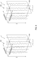
- FIGS 1A-1B show side-elevation and top views, respectively, of an example seismic data acquisition system that comprises a survey vessel 102 towing a source 104 and six separate streamers 106-111 beneath a free surface 112 of a body of water.
- the body of water can be, for example, an ocean, a sea, a lake, or a river, or any portion thereof.
- each streamer is attached at one end to the survey vessel 102 via a streamerdata-transmission cable.
- the illustrated streamers 106-111 form an ideally planar horizontal data acquisition surface with respect to the free surface 112.
- the data acquisition surface may be smoothly varying due to active sea currents and weather conditions.
- the streamers 106-111 are illustrated in Figures 1A and 1B and subsequent figures as straight and approximately parallel to the free surface 112, in practice, the towed streamers may undulate because of dynamic conditions of the body of water in which the streamers are submerged.
- a data acquisition surface is not limited to having a planar horizontal orientation with respect to the free surface 112. The streamers may be towed at depths that angle the data acquisition surface with respect to the free surface 112 or one or more of the streamers may be towed at different depths.
- a data acquisition surface is not limited to six streamers as shown in Figure 1B . In practice, the number of streamers used to form a data acquisition surface can range from as few as one streamer to as many as 20 or more streamers.
- the source 104 comprises an array of source elements, such as air guns or the source 104 may be a marine vibrator.
- Figure 1A includes an xz -plane 114 and Figure 1B includes an xy- plane 116 of the same Cartesian coordinate system having three orthogonal, spatial coordinate axes labeled x, y and z.
- the coordinate system specifies orientations and coordinate locations within the body of water.
- the x-direction specifies the position of a point in a direction parallel to the length of the streamers or in the direction the survey vessel is traveling and is referred to as the "in-line" direction.
- the y -direction specifies the position of a point in a direction perpendicular to the x -axis and approximately parallel to the free surface 112 and is referred to as the "cross-line" direction.
- the z -direction specifies the position of a point perpendicular to the xy -plane (i.e., perpendicular to the free surface 112) with the positive z-direction pointing downward away from the free surface 112.
- the streamers 106-111 are long cables containing power and data-transmission lines that connect receivers represented by shaded rectangles, such as receiver 118, spaced-apart along the length of each streamer to seismic acquisition equipment and data-storage devices located on board the survey vessel 102.
- Streamer depth below the free surface 112 can be estimated at various locations along the streamers using depth-measuring devices attached to the streamers.
- the depth-measuring devices can measure hydrostatic pressure or utilize acoustic distance measurements.
- the depth-measuring devices may be integrated with depth controllers, such as paravanes or water kites that control and maintain the depth and position of the streamers as the streamers are towed through the body of water.
- the depth-measuring devices are typically placed at intervals (e.g., about 300 meter intervals in some implementations) along each streamer. Note that in other implementations buoys may be attached to the streamers and used to maintain the orientation and depth of the streamers below the free surface 112.
- Figure 1A shows a cross-sectional view of the survey vessel 102 towing the source 104 above a subterranean formation 120.
- Curve 122 the formation surface, represents a top surface of the subterranean formation 120 located at the bottom of the body of water.
- the subterranean formation 120 has a number of subterranean layers of sediment and rock.
- Curves 124, 126, and 128 represent interfaces between subterranean layers of different compositions.
- a shaded region 130, bounded at the top by a curve 132 and at the bottom by a curve 134, represents a subterranean hydrocarbon deposit, the depth and positional coordinates of which may be determined, at least in part, by analysis of seismic data collected during a marine seismic survey.
- the source 104 may be activated to produce acoustic signals at spatial and/or temporal intervals. Activation the source 104 is often called a "shot.” In other implementations, the source 104 may be towed by one survey vessel and the streamers may be towed by a different survey vessel.
- Figure 1A shows an acoustic signal expanding outward from the source 104 as a pressure wavefield 136 represented by semicircles of increasing radius centered at the source 104. The outwardly expanding wavefronts from the source 104 may be spherical but are shown in vertical plane cross section in Figure 1A .
- the outward and downward expanding portion of the pressure wavefield 136 and any portion of the pressure wavefield 136 reflected from the free-surface 112 are called the "source signal.”
- the source signal eventually reaches the formation surface 122 of the subterranean formation 120, at which point the source signal may be partially reflected from the formation surface 122 and partially refracted downward into the subterranean formation 120, becoming elastic waves within the subterranean formation 120.
- the acoustic signal is primarily comprised of compressional pressure waves, or P-waves, while in the subterranean formation 120, the waves include both P-waves and transverse waves, or S-waves.
- each point of the formation surface 122 and each point of the interfaces 124, 126, and 128 may be a reflector that becomes a potential secondary point source from which acoustic and elastic wave energy, respectively, may emanate upward toward the receivers 118 in response to the acoustic signal generated by the source 104 and downward-propagating elastic waves generated from the pressure impulse.
- waves of significant amplitude may be generally reflected from points on or close to the formation surface 122, such as point 138, and from points on or very close to interfaces in the subterranean formation 120, such as points 140 and 142.
- the upward expanding waves emanating from the subterranean formation 120 are collectively the "reflected wavefield.”
- the waves that comprise the reflected wavefield may be generally reflected at different times within a range of times following the initial source signal.
- a point on the formation surface 122 such as the point 138, may receive a pressure disturbance from the source signal more quickly than a point within the subterranean formation 120, such as points 140 and 142.
- a point on the formation surface 122 directly beneath the source 104 may receive the pressure disturbance sooner than a more distant-lying point on the formation surface 122.
- the times at which waves are reflected from various points within the subterranean formation 120 may be related to the distance, in three-dimensional space, of the points from the activated source 104.
- the travel times of the source signal and reflected wavefield may be functions of distance from the source 104 as well as the materials and physical characteristics of the materials through which the wavefields travel.
- expanding wavefronts of the wavefields may be altered as the wavefronts cross interfaces and as the velocity of sound varies in the media traversed by the wavefronts.
- the superposition of waves reflected from within the subterranean formation 120 in response to the source signal may be a generally complicated wavefield that includes information about the shapes, sizes, and material characteristics of the subterranean formation 120, including information about the shapes, sizes, and locations of the various reflecting features within the subterranean formation 120 of interest to exploration seismologists.
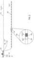
- Figure 2 shows a side-elevation view of the seismic data acquisition system with a magnified view 202 of the receiver 118.
- the magnified view 202 reveals that the receiver 118 is a multi-component sensor that comprises a pressure sensor 204 and a particle motion sensor 206.
- the pressure sensor may be, for example, a hydrophone.
- Each pressure sensor is a non-directional sensor that measures changes in hydrostatic pressure over time to produce pressure data denoted p x ⁇ S x ⁇ R t , where x ⁇ S represents source 104 coordinates ( x s , y s , z s ), x ⁇ R represents receiver 118 coordinates ( x R , y R , z R ), and t represents time.
- the particle motion sensors may be responsive to water motion.
- the term "particle motion sensor” is a general term that refers to a sensor configured to detect particle displacement, particle velocity, or particle acceleration over time. In general, particle motion sensors detect particle motion in a particular direction and may be responsive to such directional displacement of the particles, velocity of the particles, or acceleration of the particles.
- a particle motion sensor that measures particle displacement generates particle displacement data denoted by g n ⁇ x ⁇ S x ⁇ R t , where the vector n ⁇ represents the direction along which particle displacement is measured.
- a particle motion sensor that measures particle velocity i.e., particle velocity sensor
- a particle motion sensor that measures particle acceleration i.e., accelerometer
- a particle motion sensor that measures particle acceleration generates particle acceleration data denoted by a n ⁇ x ⁇ S x ⁇ R t .
- the data generated by one type of particle motion sensor may be converted to another type. For example, particle displacement data may be differentiated to obtain particle velocity data, and particle acceleration data may be integrated to obtain particle velocity data.
- particle motion data is a general term that refers to particle displacement data, particle velocity data, or particle acceleration data
- semiconductor data refers to pressure data and/or particle motion data.
- the pressure data represents a pressure wavefield
- particle displacement data represents a particle displacement wavefield
- particle velocity data represents a particle velocity wavefield
- particle acceleration data represents particle acceleration wavefield.
- the particle displacement, velocity, and acceleration wavefields are referred to as particle motion wavefields.
- each receiver may include three particle motion sensors that measure particle motion in three orthogonal directions.
- each receiver may include a particle motion sensor that measures the wavefield in the in-line direction in order to obtain the inline velocity data, v x x ⁇ S x ⁇ R t , and a particle motion sensor that measures the wavefield in the cross-line direction in order to obtain the cross-line velocity data, v y x ⁇ S x ⁇ R t .
- the receivers may comprise only pressure sensors, and in other implementations, the receivers may comprise only particle motion sensors.
- the streamers 106-111 and the survey vessel 102 may include sensing electronics and data-processing facilities that allow seismic data generated by each receiver to be correlated with the time when the source 104 is activated, absolute positions on the free surface 112, and absolute three-dimensional positions with respect to an arbitrary three-dimensional coordinate system.
- the pressure data and particle motion data may be stored at the receiver, and/or may be sent along the streamers and data transmission cables to the survey vessel 102, where the data may be stored electronically or magnetically on data-storage devices located onboard the survey vessel 102 and/or transmitted onshore to a seismic data-processing facility.
- Each pressure sensor and particle motion sensor may include an analog-to-digital converter that converts time-dependent analog signals into discrete time series data that consist of a number of consecutively measured values called "amplitudes" separated in time by a sample rate.
- the pressure or particle motion data generated by a pressure sensor or a particle motion sensor is time series data and is called a "trace," which may consist of thousands of samples collected at a typical sample rate of about 1 to 5 ms.
- a trace is a recording of a subterranean formation response to acoustic energy that passes from an activated source, into the subterranean formation where a portion of the acoustic energy is reflected and/or refracted, and ultimately detected by a sensor as described above.
- a trace records variations in a time-dependent amplitude that corresponds to fluctuations in acoustic energy of the wavefield measured by the sensor.
- a reflected wavefield that emanates from the subterranean formation may undergo different reflection events before being measured by the receivers. For example, a portion of the reflected wavefield may travel directly from the subterranean formation to the receivers. However, because the free surface acts as a nearly perfect reflector other portions of the reflected wavefield may be reflected a number of times between the free surface and the subterranean formation before being measured by the receivers. The reflected wavefield may have also been reflected a number of times between different interfaces within the subterranean formation before entering the body of water.
- Figures 3A-3C show a number of ways acoustic energy reverberates between the free surface and the subterranean formation before being measured at the receiver 118.
- directional arrows 301-306 represent ray paths of different portions of the source signal generated by the source 104 that reach different interfaces within the subterranean formation 102 before being reflected.
- ray path 301 represents a portion of the acoustic energy in the source signal that reaches the interface 128
- ray path 306 represents a portion of the acoustic energy in the source signal that reaches the formation surface 122.
- ray paths 304 and 306 represent reflections from the interface 124 and the formation surface 122 that travel directly to the receiver 118, which are called “up-going primary reflections” as indicated by directional arrow 316.
- Ray paths 303 and 305 represent reflections from the interface 124 and the formation surface 122 followed by reflections from the free surface 112 before traveling directly to the receiver 118, which are called “down-going primary reflections” as indicated by directional arrow 318.
- ray paths 301 and 302 represent multiple reflections between interfaces within the subterranean formation 120 and the free surface 112.
- Ray path 301 represent a down-going multiple as represented by directional arrow 318.
- Ray path 302 represents an up-going multiple as represented by directional arrow 316.
- Each trace records the primaries and various types of multiples.
- pressure data p x ⁇ S x ⁇ R t generated at the receiver 118 records the primary and multiple reflections
- vertical velocity data v Z x ⁇ S x ⁇ R t also generated at the receiver 118 records the primary and multiple reflections.
- the pressure data p x ⁇ S x ⁇ R t and the vertical velocity data v Z x ⁇ S x ⁇ R t comprise both up-going and down-going pressure and vertical velocity wavefields, respectively, that reach the receiver 118.
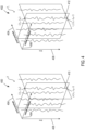
- Figure 4 shows a set of pressure data 400 collected for a number of different source and receiver coordinate locations and a set of vertical velocity data 402 collected for the same source and receiver coordinate locations.
- Axis 404 represents source coordinates
- axis 406 represents receiver coordinates
- axis 408 represents time.
- Wiggle lines represent traces of pressure and vertical velocity data generated by collocated pressure and vertical velocity sensors and different locations for each source activation.
- a wiggle line 410 represents a trace of pressure data p x ⁇ S x ⁇ R t , as described above with reference to Equation (1), recorded for a source activated at a source location x ⁇ S and a pressure sensor at a receiver location x ⁇ R .
- a wiggle line 412 represents a trace of vertical velocity data v Z x ⁇ S x ⁇ R t , as described above with reference to Equation (1), recorded for the same source and receiver coordinate locations.
- the traces in the sets of pressure and vertical velocity data 400 and 402 may be sorted into different domains, such as the common-shot domain, common-receiver-station domain, common-channel domain, and common-midpoint domain.
- the sets of pressure data and vertical velocity data may be transformed from the space-time (“s-t") domain to the wavenumber-frequency (“w-f") domain using a fast Fourier transform (“FFT”) or a discrete Fourier transform (“DFT”) as follows: p x ⁇ S x ⁇ R t ⁇ P k ⁇ R , z R
- V z k ⁇ R , z R 0
- x ⁇ S , ⁇ V z k ⁇ R , z R
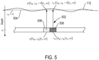
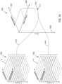
- Figure 5 shows an example of extrapolating pressure and vertical velocity data generated by collocated pressure and particle motion sensors of a receiver 502 to the free surface 112.
- the receiver 502 with collocated pressure sensor 506 and particle motion sensor 508 is located at a depth z R below the free surface 112. Note that in the following description, unless otherwise stated, the depth coordinate z R is equal to zero.
- Figure 6 shows a set of pressure data 600 in the w-f domain and a set of vertical velocity data 602 in the w-f domain.
- Axis 604 represents a range of angular frequencies denoted by ⁇ .
- Axis 606 represent receiver wavevector coordinates k ⁇ R z R .
- Layers in the set of pressure data 600 represent matrices, or frequency slices, of pressure data that have the same angular frequency.
- Layers in the set of vertical velocity data 602 represent matrices, or frequency slices, of vertical velocity data that have the same angular frequency.
- shaded layer 608 represents a matrix or frequency slice of pressure data over the range of source and receiver wavevector coordinates at angular frequency ⁇ '
- shaded layer 612 represents a matrix or frequency slice of vertical velocity data over the range of source and receiver wavevector coordinates at the same angular frequency ⁇ '
- Points 610 and 614 represent pressure and vertical velocity amplitudes with the same source and receiver wavevector coordinates and the same angular frequency denoted by k ⁇ R , z R
- x ⁇ S , ⁇ and the set of vertical velocity data 602 in the w-f domain is represented by: V ⁇ z V z k ⁇ R , z R
- Wavefield separation may be used to decompose the set of pressure data into a set of up-going pressure data and a set of down-going pressure data.
- the down-going pressure data is calculated as follows: P d k ⁇ R , z R
- x ⁇ S , ⁇ 1 2 P k ⁇ R , z R
- x ⁇ S , ⁇ 1 2 P k ⁇ R , z R
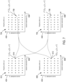
- Figure 7 shows a plot of the frequency slice 608 of pressure data and a plot of the frequency slice 612 of vertical velocity data described above with reference to Figure 6 .
- Points in plots 608 and 612 represent corresponding pressure and vertical velocity amplitudes at the same angular frequency ⁇ ' and the same source coordinates and receiver wavevector coordinates.
- point 610 represents pressure data P k ⁇ R , z R
- point 614 represents vertical velocity data V z k ⁇ R , z R
- Figure 7 also shows plots of frequency slices of up-going pressure data 702 and down-going pressure data 704 for the same angular frequency ⁇ ' and source coordinates and receiver wavenumber coordinates.
- point 706 represents the up-going pressure data P u k ⁇ R , z R
- Point 708 represents the down-going pressure data P d k ⁇ R , z R
- Figure 8 shows a set of up-going pressure data 800 and a set of down-going pressure data 802 in the w-f domain.
- Layers in the set of pressure data 802 represent matrices or frequency slices of up-going pressure data with the same angular frequency
- layers in the set of down-going data 802 represent matrices or frequency slices of down-going pressure data with the same angular frequency.
- shaded layers 804 and 806 represent frequency slice 702 of up-going pressure data and frequency slice 704 of down-going pressure data, respectively, in Figure 7 .
- x ⁇ S , ⁇ and the set of down-going pressure data 802 in the w-f domain is represented by: P ⁇ d P d k ⁇ R , z R
- the set of up-going pressure data P u and the set of down-going pressure data P d data may be inverse transformed from the w-f domain to the s-t domain using a fast inverse Fourier transform ("IFFT”) or an inverse discrete Fourier transform (“IDFT”) as follows: P u k ⁇ R , z R
- FIG 9 shows a set of up-going going pressure data 900 and a set of down-going pressure data 902 in the s-t domain.
- Wiggle lines represent traces of up-going and down-going components of the pressure data 400.
- wiggle line 904 represents a trace of up-going pressure data p u x ⁇ S x ⁇ R t
- wiggle line 906 represents a trace of down-going pressure data p d x ⁇ S x ⁇ R t
- the trace 904 of up-going pressure data p u x ⁇ S x ⁇ R t represents the up-going pressure wavefield portion of the trace 410 of the pressure data p x ⁇ S x ⁇ R t in Figure 4 .
- the trace 905 of down-going pressure data p d x ⁇ S x ⁇ R t represents the down-going pressure wavefield portion of the trace 412 of the pressure data p x ⁇ S x ⁇ R t in Figure 4 .
- the up-going pressure data p u x ⁇ S x ⁇ R t represents the portion of the reflected wavefield recorded in the pressure data p x ⁇ S x ⁇ R t that travels upward to the receiver 118 as represented by directional arrow 316 in Figure 3 .
- the down-going pressure data p d x ⁇ S x ⁇ R t represents the down-going pressure wavefield portion of the trace of pressure data p x ⁇ S x ⁇ R t that travels downward to the receiver 118 as represented by directional arrow 318 of Figure 3 .
- the in-line and cross-line receiver coordinates record the actual locations of receivers in real world conditions, the in-line and cross-line receiver coordinates are not regularly spaced apart, and therefore do not conform to regularly spaced grid points of a migration grid.
- the in-line and cross-line receiver coordinates of the set of up-going pressure data 900 and the set of down-going pressure data 902 are regularized to match the regularly spaced grid points of a migration grid.
- the in-line and cross-line coordinates of the receivers of the up-going and down-going pressure data may be regularized by moving the in-line and cross-line coordinates to the closest regularly spaced grid points of the migration grid.
- Regularization may be used to move irregularly spaced receiver coordinates to a set of regularly spaced grid points of a migration grid.
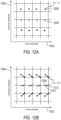
- Figures 10A-10B show an example of regularization of irregularly spaced receiver coordinates to regularly spaced grid points of a migration grid.
- Figure 10A shows an example of irregularly spaced receiver coordinates and an overlay of regularly spaced grid lines of a migration grid.
- Axis 1002 represents in-inline receiver coordinate x R .
- Axis 1004 represents cross-line receiver coordinate y R .
- Points represent in-line and cross-line receiver coordinates of the eight receivers of a seismic data acquisition system.
- point 1006 represents in-line and cross-line receiver coordinates ( x R , y R ) of a receiver.
- the in-line and cross-line receiver coordinates of the receivers are irregularly spaced apart, which may be due to currents, waves, and changing conditions of the body of water.
- Vertical and horizontal lines such as vertical line 1008 and horizontal line 1010, represent regularly spaced grid lines (i.e., in-line and cross-line) of a migration grid.
- d 1 , d 2 , d 3 , and d 4 represent distances from the point 1006 to the four nearest grid points of the migration grid.
- the irregularly spaced receiver coordinates may be regularized to nearest grid points as shown in Figure 10B .
- Directional arrows represent regularizing the irregularly spaced receiver coordinates to nearest grid points of the migration grid.
- directional arrow 1014 represents regularizing the receiver coordinate 1006 to a grid point 1016 of the migration grid.
- the regularly spaced receiver coordinates at grid points of the migration grid are denoted by ( x' R , y' R ) and called "receiver migration grid coordinates.”
- the receivers located along the streamers are spaced apart by about 12 meters to about 13 meters along the streamers in the in-line direction while adjacent streamers may be separated by anywhere from about 75 meters to about 100 meters or more.
- reflected wavefields sampled by the receivers may be spatially aliased in the cross-line direction.
- certain recorded traces may be corrupted or omitted because of problems with pressure and/or particle motion sensors. Interpolation may be used to fill in missing traces of up-going and down-going pressure data in the cross-line direction and replace any corrupted or missing traces of up-going and down-going pressure data in the in-line direction.
- Figures 11A-11C show interpolation of traces of up-going and down-going pressure data at grid points of a migration grid.
- Figure 11A shows a plot of regularized receiver coordinates at grid points of a migration grid.
- Axis 1102 represents in-line receiver coordinate x R .
- Axis 1104 represents cross-line receiver coordinate y R .
- Vertical and horizontal lines, such as vertical line 1106 and horizontal line 1108, represent regularly spaced grid lines of the migration grid. Intersections between vertical and horizontal grid lines, such as intersection 1110, represent regularly spaced grid points of the migration grid.
- Points, such as point 1112, located at grid points represent regularized receiver coordinates of up-going and down-going pressure data.
- Interpolation may be used to fill in traces of up-going and down-going pressure data at grid points from nearest traces of up-going and down-going pressure data at regularized receiver coordinates.
- the traces of up-going pressure data (and down-going pressure data) at regularized receiver coordinates that lie within a circle 1114 of radius r and centered at grid point 1116 may be used to interpolate a trace of up-going pressure data (and down-going pressure data) at the grid point 1116.
- the traces located closer to the grid point 1116 may be given more weight than traces located farther away from the grid point.
- dotted wiggle line 1118 represents an interpolated trace of up-going pressure data (down-going pressure data) at a grid point 1119.
- the interpolated trace 1118 of up-going pressure data (down-going pressure data) is calculated from six nearest traces 1120-1125 of up-going pressure data (down-going pressure data).
- the traces 1123-1125 may be given more weight in the interpolation of the interpolated trace 1118 than the traces 1120-1122 because the regularized coordinates of the traces 1123-1125 are closer to the grid point 1119 than the regularized coordinates of the traces 1120-1122.
- Open circles at grid points in Figure 11C represent regularly spaced receiver coordinates of interpolated traces of up-going and down-going pressure data.
- Regularization and interpolation may be accomplished with an anti-leakage Fourier transform.
- Other regularization and interpolation techniques include linear moveout with bilinear interpolation, three-dimensional interpolation, and five-dimensional interpolation.
- interpolation may be applied first to interpolate up-going pressure data (down-going pressure data) from the irregularly spaced up-going pressure data (down-going pressure data) followed by regularization of the interpolated and known up-going pressure data (down-going pressure data).
- Figure 12A shows points, such as point 1202, that represent irregularly spaced receiver coordinates of up-going pressure data (down-going pressure data).
- Open circles, such as open circle 1208, represent receiver coordinates of interpolated pressure data (down-going pressure data) from nearest known up-going pressure data (down-going pressure data), as described above with reference to Figure 11B .
- the irregularly spaced receiver coordinates of up-going pressure data (down-going pressure data) may be regularized to nearest grid points as shown in Figure 12B .
- Directional arrows represent regularizing the irregularly spaced receiver coordinates of up-going pressure data (down-going pressure data) to nearest grid points of the migration grid, as described above with reference to Figures 10A-10B .
- directional arrow 1210 represents regularizing the receiver coordinate 1208 to a grid point 1212 of the migration grid.
- Figure 13 shows a set of interpolated and regularized up-going pressure data 1300 and a set of interpolated and regularized down-going pressure data 1302 in the s-t domain.
- Dashed wiggle line 1304 represents an interpolated trace of up-going pressure data p u x ⁇ S , x ⁇ ′ Ra , t
- wiggle line 1306 represents a regularized trace of up-going pressured data p u x ⁇ S , x ⁇ ′ Rb , t .
- Dashed wiggle line 1308 represents an interpolated trace of down-going pressure data p d x ⁇ S , x ⁇ ′ Ra , t
- wiggle line 1310 represents a regularized trace of down-going pressured data p d x ⁇ S , x ⁇ ′ Rb , t .
- the set of interpolated and regularized up-going pressure data 1200 and set of interpolated and regularized down-going pressure data 1202 are transformed from the s-t domain to the space-frequency ("s-f") domain using an FFT or a DFT as follows: p u x ⁇ S , x ⁇ ′ R , t ⁇ P u x ⁇ S , x ⁇ ′ R , ⁇ p d x ⁇ S , x ⁇ ′ R , t ⁇ P d x ⁇ S , x ⁇ ′ R , ⁇
- the sets of interpolated and regularized up-going pressure data and down-going pressure data in the s-f domain are used to calculate a seismic image using an image condition.
- the down-going pressure wavefield P d x ⁇ S , x ⁇ ′ R , ⁇ may be referred to as an input for a source wavefield
- the up-going pressure wavefield P u x ⁇ S , x ⁇ ′ R , ⁇ may be referred to as an input for a receiver wavefield.
- Different primary and multiple components in P u x ⁇ S , x ⁇ ′ R , ⁇ and P d x ⁇ S , x ⁇ ′ R , ⁇ as represented in Equations (13a) and (13b) may be combined during migration to generate a seismic image of a subterranean formation.
- the quantity I x ⁇ in Equation (14) is an image value of the seismic image at the grid point x ⁇ of the migration grid.
- migration generates pixels of a seismic image by calculating the image value I x ⁇ according to Equation (14) at each grid point x ⁇ of the migration grid.
- Each pixel of the seismic image comprises a grid point x ⁇ and an image value I x ⁇ .
- Figure 14 shows calculation of a seismic image from a set of interpolated and regularized up-going pressure data 1400 and a set of interpolated and regularized down-going pressure data 1402 in the s-f domain.
- Figure 14 also show a seismic image coordinate system 1404.
- Directional arrows 1406-1408 represents the x- , y- , and z- axes of the seismic image coordinate system 1404.
- Point 1410 represents a grid point x ⁇ .
- Dotted lines 1412 and 1414 represent using the entire set of up-going pressure data P ⁇ u and the entire of set of down-going pressure data P ⁇ d in Equation (12) to calculate an image value I x ⁇ of a seismic image at the grid point x ⁇ 1410.
- the image value I x ⁇ and the grid point x ⁇ 1410 are a pixel of the seismic image.
- An image values may be calculated for each grid point of the image coordinate system 1404 to form a seismic image of a subterrane
- Crosstalk effects may be created when source wavefields (i.e., down-going pressure wavefield P d x ⁇ S , x ⁇ ′ R , ⁇ ) and receiver wavefield (i.e., up-going pressure wavefield P u x ⁇ S , x ⁇ ′ R , ⁇ ) are in phase at locations with a subterranean formation that are not the same location as a subterranean formation interface.
- the amount of error created by crosstalk depends on the location of the boundary receiver wavefield and if it is surface consistent, making the crosstalk artifacts from different shot records incoherent.
- Adding fold by receiver wavefield interpolation and regularization may attenuate the incoherent crosstalk artifacts during migration.
- the interpolated and regularized receive wavefield i.e., up-going pressure wavefield P u x ⁇ S , x ⁇ ′ R , ⁇
- the coherent signal component is improved by stacking and the adverse effects of incoherent crosstalk artifacts are weakened.
- Figure 15 shows a flow diagram of a method to generate a seismic image.
- a set of pressure data and a set of vertical velocity data generated by collocated pressure and particle motion sensors of a seismic data acquisition system are received.
- a routine to "separate pressure data into up-going pressure data and down-going pressure data wavefield" based on the set of pressure data and the set of vertical velocity data is called.
- a routine "generate a set of interpolated and regularized down-going pressure data" at grid points of a migration grid is called.
- a routine "generate a set of interpolated and regularized up-going pressure data" at grid points of the same migration grid is called.
- a routine "calculate seismic image on migration grid” is called to calculate a seismic image based on the regularized and interpolated down-going and up-going pressure data.
- Figure 16 shows a flow diagram of the method to "separate pressure data into up-going pressure data and down-going pressure data" called in block 1502 of Figure 15 .
- the set of pressure data and the set of vertical velocity data are transformed from the s-t domain to the w-f domain as described with reference to Equations (3a) and (3b).
- the sets of pressure and vertical velocity data are extrapolated from receiver depth to the level of the free surface, as described above with reference to Figure 5 and Equations (4a) and (4b).
- a set of down-going pressure data is calculated from the set of pressure data and the set of vertical velocity data as described above with reference to Equation (6a).
- the set of down-going pressure data is transformed back to the s-t domain, a described above with reference to Equation (8a).
- a set of up-going pressure data is calculated from the set of pressure data and the set of vertical velocity data as described above with reference to Equation (6b).
- the set of up-going pressure data is transformed back to the s-t domain, a described above with reference to Equation (8b).
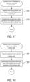
- Figure 17 shows a flow diagram of the method "generate a set of interpolated and regularized down-going pressure data" called in block 1503 of Figure 15 .
- irregular receiver coordinates of the down-going pressure data are regularized to grid points of the migration grid, as described above with reference to Figures 10A-10B .
- down-going pressure data is interpolated at grid points of the migration grid from the down-going pressure data regularized to grid points of migration grid to generate a set of interpolated and regularized down-going pressure data at grid points of the migration grid, as described above with reference to Figures 1 1A-11C .
- Figure 18 shows a flow diagram of the method "generate a set of interpolated and regularized up-going pressure data" called in block 1504 of Figure 15 .
- irregular receiver coordinates of the up-going pressure data are regularized to grid points of the migration grid, as described above with reference to Figures 10A-10B .
- up-going pressure data is interpolated at grid points of the migration grid from the up-going pressure data regularized to grid points of migration grid to generate a set of interpolated and regularized up-going pressure data at grid points of the migration grid, as described above with reference to Figures 1 1A-11C .
- Figure 19 shows a control-flow diagram of the method "calculate seismic image on migration grid" called in block 1505 of Figure 15 .
- the set of interpolated and regularized down-going pressure data is transformed from the s-t domain to the s-f domain, as described above with reference to Equation (12b).
- the set of interpolated and regularized up-going pressure data is transformed from the s-t domain to the s-f domain, as described above with reference to Equation (12a).
- a for-loop beginning with block 1903 repeats the calculation of block 1904 for each grid point of the migration grid.
- an seismic image value is calculated according to Equation (14) at a grid point, as described above with reference to Equation (14) and represented in Figure 14 .
- decision block 1905 the calculation represented by block 1904 is repeated.
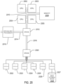
- Figure 20 shows an example of a computer system that executes efficient methods of calculating a seismic image and therefore represents a geophysicalanalysis data-processing system.
- the internal components of many small, mid-sized, and large computer systems as well as specialized processor-based storage systems can be described with respect to this generalized architecture, although each particular system may feature many additional components, subsystems, and similar, parallel systems with architectures similar to this generalized architecture.
- the computer system contains one or multiple central processing units ("CPUs") 2002-2005, one or more electronic memories 2008 interconnected with the CPUs by a CPU/memory-subsystem bus 2010 or multiple busses, a first bridge 2012 that interconnects the CPU/memory-subsystem bus 2010 with additional busses 2014 and 2016, or other types of high-speed interconnection media, including multiple, high-speed serial interconnects.
- CPUs central processing units
- electronic memories 2008 interconnected with the CPUs by a CPU/memory-subsystem bus 2010 or multiple busses
- a first bridge 2012 that interconnects the CPU/memory-subsystem bus 2010 with additional busses 2014 and 2016, or other types of high-speed interconnection media, including multiple, high-speed serial interconnects.
- the busses or serial interconnections connect the CPUs and memory with specialized processors, such as a graphics processor 2018, and with one or more additional bridges 2020, which are interconnected with high-speed serial links or with multiple controllers 2022-2027, such as controller 2027, that provide access to various different types of computer-readable media, such as computer-readable medium 2028, electronic displays, input devices, and other such components, subcomponents, and computational resources.
- the electronic displays including visual display screen, audio speakers, and other output interfaces, and the input devices, including mice, keyboards, touch screens, and other such input interfaces, together constitute input and output interfaces that allow the computer system to interact with human users.
- Computer-readable medium 2028 is a data-storage device, including electronic memory, optical or magnetic disk drive, USB drive, flash memory and other such data-storage device.
- the computer-readable medium 2028 can be used to store machine-readable instructions that encode the computational methods described above and can be used to store encoded data, during store operations, and from which encoded data can be retrieved, during read operations, by computer systems, data-storage systems, and peripheral devices.
- Figures 21A-21B show a time slice of a common-shot gather before ( Figure 21A ) and after interpolation ( Figure 21B ).
- horizontal axis 2102 represents the in-line direction and vertical axis 2104 represents the cross-line direction.
- lines of common-shot seismic data such as line of seismic data 2106, are separate by gaps 2108 that correspond to larger cross-line separation distances (e.g., about 75-100 meters) between adjacent streamers as compared to much short separation distances between receivers located along the streamers (e.g., about 12.5 meters).
- Figure 21B reveals how regularization and interpolation using an anti-leakage Fourier transform filled in the gaps between receivers in the cross-line direction.
- Figures 22A-22B show depth slices of seismic images generated using a source wavefield without regularization and interpolation ( Figure 22A ) and using a source wavefield with regularization and interpolation ( Figure 22B ).
- the streamers are separated by 100 meters.
- interpolation has been used to generate interpolated seismic data at 25 meters spacings between streamers.
- Figure 22B shows a higher-resolution and higher signal-to-noise seismic image than the seismic image shown in Figure 22A .
- Figures 23A-23B show depth slices of seismic images generated using a receiver wavefield without regularization and interpolation ( Figure 23A ) and using a receiver wavefield with regularization and interpolation ( Figure 23B ).
- Receiver wavefield interpolation and regularization attenuates crosstalk artifacts.
- circled regions 2302, 2304, and 2306 identify regions that display crosstalk artifacts.
- the crosstalk artifacts are removed as a result receiver wavefield regularization and interpolation.
- Figure 23B shows a higher-resolution seismic image than the seismic image shown in Figure 23A .
- the methods and systems described above produce high-resolution seismic images of a subterranean formation with seismic data that records both primaries and multiples.
- the high-resolution seismic images may, in turn, be used to determine the structure of the subterranean formation.
- the structural information may reveal how different rock, sediment, and hydrocarbon deposits are organized within the formation, may reveal the location of possible hydrocarbon deposits, and may be used to monitor existing hydrocarbon deposits during production.
- the methods and systems described above may be used to manufacture a geophysical data product indicative of certain properties of a subterranean formation.
- the geophysical data product may include geophysical data such as pressure data, particle motion data, particle velocity data, particle acceleration data, and any seismic image that results from using the methods and systems described above.
- the geophysical data product may be stored on a non-transitory computer-readable medium as described above.
- the geophysical data product may be produced offshore (i.e., by equipment on the survey vessel 102) or onshore (i.e., at a computing facility on land) either within the United States or in another country. When the geophysical data product is produced offshore or in another country, it may be imported onshore to a data-storage facility in the United States. Once onshore in the United States, geophysical analysis may be performed on the geophysical data product.
Landscapes
- Life Sciences & Earth Sciences (AREA)
- Physics & Mathematics (AREA)
- Remote Sensing (AREA)
- Engineering & Computer Science (AREA)
- Geology (AREA)
- Environmental & Geological Engineering (AREA)
- Acoustics & Sound (AREA)
- General Life Sciences & Earth Sciences (AREA)
- General Physics & Mathematics (AREA)
- Geophysics (AREA)
- Oceanography (AREA)
- Geophysics And Detection Of Objects (AREA)
- Image Processing (AREA)
- Measurement Of Mechanical Vibrations Or Ultrasonic Waves (AREA)
Description
- Marine seismology companies invest heavily in the development of marine seismic surveying equipment and seismic data processing techniques in order to obtain accurate, high-resolution seismic images of subterranean formations located beneath a body of water. High-resolution seismic images are used to determine the structure of subterranean formations, discover hydrocarbon deposits, and monitor hydrocarbon deposits during production. A typical marine seismic survey is carried out with a survey vessel that tows one or two seismic sources and a number of streamers below the surface of the body of water. A typical seismic source comprises an array of source elements, such as air guns. The streamers are elongated cable-like structures towed behind the survey vessel in the direction the survey vessel is traveling. Each streamer includes a number of receivers that generate seismic data in response to detecting pressure and/or particle motion wavefields. The streamers are arranged substantially parallel to one another to form a seismic data acquisition system. The survey vessel contains seismic acquisition equipment, such as navigation control, seismic source control, seismic receiver control, and seismic data recording equipment.
- A typical marine seismic survey is carried out by activating the one or more seismic sources above a subterranean formation. Each activation produces an acoustic signal that expands outward in all directions. A portion of the acoustic signal travels downward through the body of water and into the subterranean formation. At each interface between different types of rock and sediment, a portion of the acoustic signal is refracted, a portion is transmitted, and another portion is reflected back from each interface into the body of water to propagate toward the free surface. The portion of the acoustic signal reflected back into the body of water and that travels directly to the receivers is called a primary reflected wavefield or simply a primary. Other portions of the acoustic signal that is reflected back into the body of water may be reflected a number of times between the free surface and between interfaces within the subterranean formation before reaching the receivers. These multiple reflected wavefields are called multiples. Multiples are typically treated as noise and are suppressed in seismic imaging. In recent years, multiples have been recognized as containing valuable information about the subterranean formation. As a result, techniques have been developed to generate seismic images from both primaries and multiples. However, the resulting seismic images typically have a low signal-to-noise ratio and are often contaminated with adverse crosstalk effects, which lowers the resolution of the seismic images.
-
US 2014/0119157 A1 discusses the separation and interpolation of up-going and down-going wavefields in the context of generating a seismic image. - To address the above-mentioned problems and improve on the above-mentioned prior art, a method according to
claim 1, a system according to claim 6 and a computer-readable medium according to claim 11 are provided. -
-
Figures 1A-1B show side-elevation and top views of an example seismic data acquisition system. -
Figure 2 shows a side-elevation view of a seismic data acquisition system with a magnified view of a receiver. -
Figures 3A-3C show a number of ways acoustic energy in a reflected wavefield reverberates between the free surface and the subterranean formation. -
Figure 4 shows a set of pressure data and a set of vertical velocity data. -
Figure 5 shows an example of extrapolating pressure data and vertical velocity data from a receiver coordinate to the free surface. -
Figure 6 shows a set of pressure data and a set of vertical velocity data in a wavenumber-frequency domain. -
Figure 7 shows a plot of frequency slices of pressure data and vertical velocity data in the wavenumber-frequency domain. -
Figure 8 shows a set of up-going pressure data and a set of down-going pressure data in the wavenumber-frequency domain. -
Figure 9 shows a set of up-going going pressure data and a set of down-going pressure data in a space-time domain. -
Figures 10A-10B shows an example of regularizing irregularly spaced receiver coordinates to regularly spaced grid points of a migration grid. -
Figures 11A-11C show interpolation of traces of up-going and down-going pressure data at grid points of a migration grid. -
Figures 12A-12B show an example of interpolation followed by regularization of sets of up-going and down-going pressure data. -
Figure 13 shows a set of interpolated and regularized up-going going pressure data and a set of interpolated and regularized down-going pressure data in the space-time domain. -
Figure 14 shows calculation of a seismic image from a set of interpolated and regularized up-going pressure data and a set of interpolated and regularized down-going pressure data. -
Figure 15 shows a flow diagram of a method to generate a seismic image. -
Figure 16 shows a flow diagram of the method to "separate pressure data into up-going pressure data and down-going pressure data" called inFigure 15 . -
Figure 17 shows a flow diagram of the method "generate a set of interpolated and regularized down-going pressure data" called inFigure 15 . -
Figure 18 shows a flow diagram of the method "generate a set of interpolated and regularized up-going pressure data" called inFigure 15 . -
Figure 19 shows a control-flow diagram of the method "calculate seismic image on migration grid" called inFigure 15 . -
Figure 20 shows an example of a computer system that executes methods of calculating a seismic image. -
Figures 21A-21B show a time slice of a common-shot gather before and after interpolation. -
Figures 22A-22B show depth slices of seismic images generated using a source wavefield without and with regularization and interpolation. -
Figures 23A-23B show depth slices of seismic images generated using a receiver wavefield without and with regularization and interpolation. - This disclosure presents methods and systems of generating a seismic image of a subterranean formation using primaries and multiples. A set of pressure data and a set of vertical velocity data are generated by collocated pressure and particle motion sensors of streamers for one or more activations of one or more sources. The vertical velocity data is used to separate the pressure data into up-going pressure data and down-going pressure data. Irregularly spaced receiver coordinates of the down-going pressure data are regularized to grid points of a migration grid and down-going pressure data is interpolated at grid points of the migration grid. Irregularly spaced receiver coordinates of the up-going pressure data are also regularized to grid points of the same migration grid and up-going pressure data is also interpolated at grid points of the migration grid. Methods described below generate a high-resolution seismic image at grid points of the migration grid based on the interpolated and regularized up-going and down-going pressure data. The seismic image has a higher signal-to-noise ratio and fewer adverse acquisition and crosstalk effects than a similar seismic image generated by other methods. In other words, by regularizing and interpolating both the down-going and up-going pressure wavefields before imaging, the signal-to-noise ratio may be increased and many adverse acquisition and crosstalk effects are reduced.
-
Figures 1A-1B show side-elevation and top views, respectively, of an example seismic data acquisition system that comprises asurvey vessel 102 towing asource 104 and six separate streamers 106-111 beneath afree surface 112 of a body of water. The body of water can be, for example, an ocean, a sea, a lake, or a river, or any portion thereof. In this example, each streamer is attached at one end to thesurvey vessel 102 via a streamerdata-transmission cable. The illustrated streamers 106-111 form an ideally planar horizontal data acquisition surface with respect to thefree surface 112. However, in practice, the data acquisition surface may be smoothly varying due to active sea currents and weather conditions. In other words, although the streamers 106-111 are illustrated inFigures 1A and1B and subsequent figures as straight and approximately parallel to thefree surface 112, in practice, the towed streamers may undulate because of dynamic conditions of the body of water in which the streamers are submerged. A data acquisition surface is not limited to having a planar horizontal orientation with respect to thefree surface 112. The streamers may be towed at depths that angle the data acquisition surface with respect to thefree surface 112 or one or more of the streamers may be towed at different depths. A data acquisition surface is not limited to six streamers as shown inFigure 1B . In practice, the number of streamers used to form a data acquisition surface can range from as few as one streamer to as many as 20 or more streamers. Thesource 104 comprises an array of source elements, such as air guns or thesource 104 may be a marine vibrator. -
Figure 1A includes an xz-plane 114 andFigure 1B includes an xy-plane 116 of the same Cartesian coordinate system having three orthogonal, spatial coordinate axes labeled x, y and z. The coordinate system specifies orientations and coordinate locations within the body of water. The x-direction specifies the position of a point in a direction parallel to the length of the streamers or in the direction the survey vessel is traveling and is referred to as the "in-line" direction. The y-direction specifies the position of a point in a direction perpendicular to the x-axis and approximately parallel to thefree surface 112 and is referred to as the "cross-line" direction. The z-direction specifies the position of a point perpendicular to the xy-plane (i.e., perpendicular to the free surface 112) with the positive z-direction pointing downward away from thefree surface 112. The streamers 106-111 are long cables containing power and data-transmission lines that connect receivers represented by shaded rectangles, such asreceiver 118, spaced-apart along the length of each streamer to seismic acquisition equipment and data-storage devices located on board thesurvey vessel 102. - Streamer depth below the
free surface 112 can be estimated at various locations along the streamers using depth-measuring devices attached to the streamers. For example, the depth-measuring devices can measure hydrostatic pressure or utilize acoustic distance measurements. The depth-measuring devices may be integrated with depth controllers, such as paravanes or water kites that control and maintain the depth and position of the streamers as the streamers are towed through the body of water. The depth-measuring devices are typically placed at intervals (e.g., about 300 meter intervals in some implementations) along each streamer. Note that in other implementations buoys may be attached to the streamers and used to maintain the orientation and depth of the streamers below thefree surface 112. -
Figure 1A shows a cross-sectional view of thesurvey vessel 102 towing thesource 104 above asubterranean formation 120.Curve 122, the formation surface, represents a top surface of thesubterranean formation 120 located at the bottom of the body of water. Thesubterranean formation 120 has a number of subterranean layers of sediment and rock.Curves region 130, bounded at the top by acurve 132 and at the bottom by acurve 134, represents a subterranean hydrocarbon deposit, the depth and positional coordinates of which may be determined, at least in part, by analysis of seismic data collected during a marine seismic survey. As thesurvey vessel 102 moves over thesubterranean formation 120, thesource 104 may be activated to produce acoustic signals at spatial and/or temporal intervals. Activation thesource 104 is often called a "shot." In other implementations, thesource 104 may be towed by one survey vessel and the streamers may be towed by a different survey vessel.Figure 1A shows an acoustic signal expanding outward from thesource 104 as apressure wavefield 136 represented by semicircles of increasing radius centered at thesource 104. The outwardly expanding wavefronts from thesource 104 may be spherical but are shown in vertical plane cross section inFigure 1A . The outward and downward expanding portion of the pressure wavefield 136 and any portion of thepressure wavefield 136 reflected from the free-surface 112 are called the "source signal." The source signal eventually reaches theformation surface 122 of thesubterranean formation 120, at which point the source signal may be partially reflected from theformation surface 122 and partially refracted downward into thesubterranean formation 120, becoming elastic waves within thesubterranean formation 120. In other words, in the body of water, the acoustic signal is primarily comprised of compressional pressure waves, or P-waves, while in thesubterranean formation 120, the waves include both P-waves and transverse waves, or S-waves. Within thesubterranean formation 120, at each interface between different types of materials or at discontinuities in density or in one or more of various other physical characteristics or parameters, downward propagating waves may be partially reflected and partially refracted. As a result, each point of theformation surface 122 and each point of theinterfaces receivers 118 in response to the acoustic signal generated by thesource 104 and downward-propagating elastic waves generated from the pressure impulse. As shown inFigure 1A , waves of significant amplitude may be generally reflected from points on or close to theformation surface 122, such aspoint 138, and from points on or very close to interfaces in thesubterranean formation 120, such aspoints subterranean formation 120 are collectively the "reflected wavefield." - The waves that comprise the reflected wavefield may be generally reflected at different times within a range of times following the initial source signal. A point on the
formation surface 122, such as thepoint 138, may receive a pressure disturbance from the source signal more quickly than a point within thesubterranean formation 120, such aspoints formation surface 122 directly beneath thesource 104 may receive the pressure disturbance sooner than a more distant-lying point on theformation surface 122. Thus, the times at which waves are reflected from various points within thesubterranean formation 120 may be related to the distance, in three-dimensional space, of the points from the activatedsource 104. - Acoustic and elastic waves, however, may travel at different velocities within different materials as well as within the same material under different pressures. Therefore, the travel times of the source signal and reflected wavefield may be functions of distance from the
source 104 as well as the materials and physical characteristics of the materials through which the wavefields travel. In addition, expanding wavefronts of the wavefields may be altered as the wavefronts cross interfaces and as the velocity of sound varies in the media traversed by the wavefronts. The superposition of waves reflected from within thesubterranean formation 120 in response to the source signal may be a generally complicated wavefield that includes information about the shapes, sizes, and material characteristics of thesubterranean formation 120, including information about the shapes, sizes, and locations of the various reflecting features within thesubterranean formation 120 of interest to exploration seismologists. -
Figure 2 shows a side-elevation view of the seismic data acquisition system with a magnifiedview 202 of thereceiver 118. In this example, the magnifiedview 202 reveals that thereceiver 118 is a multi-component sensor that comprises apressure sensor 204 and aparticle motion sensor 206. The pressure sensor may be, for example, a hydrophone. Each pressure sensor is a non-directional sensor that measures changes in hydrostatic pressure over time to produce pressure data denoted

source 104 coordinates (xs , ys , zs ),
receiver 118 coordinates (xR , yR , zR ), and t represents time. The particle motion sensors may be responsive to water motion. The term "particle motion sensor" is a general term that refers to a sensor configured to detect particle displacement, particle velocity, or particle acceleration over time. In general, particle motion sensors detect particle motion in a particular direction and may be responsive to such directional displacement of the particles, velocity of the particles, or acceleration of the particles. A particle motion sensor that measures particle displacement generates particle displacement data denoted by


- The term "particle motion data" is a general term that refers to particle displacement data, particle velocity data, or particle acceleration data, and the term "seismic data" refers to pressure data and/or particle motion data. The pressure data represents a pressure wavefield, particle displacement data represents a particle displacement wavefield, particle velocity data represents a particle velocity wavefield, and particle acceleration data represents particle acceleration wavefield. The particle displacement, velocity, and acceleration wavefields are referred to as particle motion wavefields.
- The particle motion sensors are typically oriented so that the particle motion is measured in the vertical direction (i.e.,


- The streamers 106-111 and the
survey vessel 102 may include sensing electronics and data-processing facilities that allow seismic data generated by each receiver to be correlated with the time when thesource 104 is activated, absolute positions on thefree surface 112, and absolute three-dimensional positions with respect to an arbitrary three-dimensional coordinate system. The pressure data and particle motion data may be stored at the receiver, and/or may be sent along the streamers and data transmission cables to thesurvey vessel 102, where the data may be stored electronically or magnetically on data-storage devices located onboard thesurvey vessel 102 and/or transmitted onshore to a seismic data-processing facility. - Each pressure sensor and particle motion sensor may include an analog-to-digital converter that converts time-dependent analog signals into discrete time series data that consist of a number of consecutively measured values called "amplitudes" separated in time by a sample rate. The pressure or particle motion data generated by a pressure sensor or a particle motion sensor is time series data and is called a "trace," which may consist of thousands of samples collected at a typical sample rate of about 1 to 5 ms. A trace is a recording of a subterranean formation response to acoustic energy that passes from an activated source, into the subterranean formation where a portion of the acoustic energy is reflected and/or refracted, and ultimately detected by a sensor as described above. A trace records variations in a time-dependent amplitude that corresponds to fluctuations in acoustic energy of the wavefield measured by the sensor. In general, each trace is an ordered set of discrete spatial and time-dependent pressure or motion sensor amplitudes denoted by:

- tr represents pressure, particle displacement, particle velocity, or particle acceleration;
- A is amplitude;
- tj is the j-th sample time; and
- J is the number of time samples in the trace.
- Different portions of a reflected wavefield that emanates from the subterranean formation may undergo different reflection events before being measured by the receivers. For example, a portion of the reflected wavefield may travel directly from the subterranean formation to the receivers. However, because the free surface acts as a nearly perfect reflector other portions of the reflected wavefield may be reflected a number of times between the free surface and the subterranean formation before being measured by the receivers. The reflected wavefield may have also been reflected a number of times between different interfaces within the subterranean formation before entering the body of water.
-
Figures 3A-3C show a number of ways acoustic energy reverberates between the free surface and the subterranean formation before being measured at thereceiver 118. InFigure 3A , directional arrows 301-306 represent ray paths of different portions of the source signal generated by thesource 104 that reach different interfaces within thesubterranean formation 102 before being reflected. For example,ray path 301 represents a portion of the acoustic energy in the source signal that reaches theinterface 128 andray path 306 represents a portion of the acoustic energy in the source signal that reaches theformation surface 122. InFigure 3B ,ray paths interface 124 and theformation surface 122 that travel directly to thereceiver 118, which are called "up-going primary reflections" as indicated bydirectional arrow 316.Ray paths interface 124 and theformation surface 122 followed by reflections from thefree surface 112 before traveling directly to thereceiver 118, which are called "down-going primary reflections" as indicated bydirectional arrow 318. InFigure 3C ,ray paths subterranean formation 120 and thefree surface 112.Ray path 301 represent a down-going multiple as represented bydirectional arrow 318.Ray path 302 represents an up-going multiple as represented bydirectional arrow 316. - Each trace records the primaries and various types of multiples. For example, pressure data

receiver 118 records the primary and multiple reflections, and vertical velocity data
receiver 118 records the primary and multiple reflections. The pressure data

receiver 118. -
Figure 4 shows a set ofpressure data 400 collected for a number of different source and receiver coordinate locations and a set ofvertical velocity data 402 collected for the same source and receiver coordinate locations.Axis 404 represents source coordinates,axis 406 represents receiver coordinates, andaxis 408 represents time. Wiggle lines represent traces of pressure and vertical velocity data generated by collocated pressure and vertical velocity sensors and different locations for each source activation. For example, awiggle line 410 represents a trace of pressure data


wiggle line 412 represents a trace of vertical velocity data
pressure data 400 represented by:
vertical velocity data 402 represented by:
vertical velocity data - The sets of pressure data and vertical velocity data may be transformed from the space-time ("s-t") domain to the wavenumber-frequency ("w-f") domain using a fast Fourier transform ("FFT") or a discrete Fourier transform ("DFT") as follows:


-

- ω is the angular frequency (i.e., ω = 2πf);
- P is pressure data in the w-f domain; and
- Vz is vertical velocity data in the w-f domain.
- The pressure and vertical velocity data are extrapolated to the free surface. Extrapolation of the pressure data

pressure sensor 506 to thefree surface 112 is represented by:
- Extrapolation of the vertical velocity data

pressure sensor 506 to thefree surface 112 is represented by:
-

- c is the speed of sound in water.
-
Figure 5 shows an example of extrapolating pressure and vertical velocity data generated by collocated pressure and particle motion sensors of areceiver 502 to thefree surface 112. Dashedline 504 represents the level of the free surface, which corresponds to a depth of zR = 0. Thereceiver 502 with collocatedpressure sensor 506 andparticle motion sensor 508 is located at a depth zR below thefree surface 112. Note that in the following description, unless otherwise stated, the depth coordinate zR is equal to zero. -
Figure 6 shows a set ofpressure data 600 in the w-f domain and a set ofvertical velocity data 602 in the w-f domain.Axis 604 represents a range of angular frequencies denoted by ω.Axis 606 represent receiver wavevector coordinates
pressure data 600 represent matrices, or frequency slices, of pressure data that have the same angular frequency. Layers in the set ofvertical velocity data 602 represent matrices, or frequency slices, of vertical velocity data that have the same angular frequency. For example, shadedlayer 608 represents a matrix or frequency slice of pressure data over the range of source and receiver wavevector coordinates at angular frequency ω', and shadedlayer 612 represents a matrix or frequency slice of vertical velocity data over the range of source and receiver wavevector coordinates at the same angular frequency ω'.Points 
pressure data 600 in the w-f domain is represented by:
vertical velocity data 602 in the w-f domain is represented by:
- Wavefield separation may be used to decompose the set of pressure data into a set of up-going pressure data and a set of down-going pressure data. The down-going pressure data is calculated as follows:


-
Figure 7 shows a plot of thefrequency slice 608 of pressure data and a plot of thefrequency slice 612 of vertical velocity data described above with reference toFigure 6 . Points inplots point 610 represents pressure data
point 614 represents vertical velocity data
Figure 7 also shows plots of frequency slices of up-goingpressure data 702 and down-goingpressure data 704 for the same angular frequency ω' and source coordinates and receiver wavenumber coordinates. For example,point 706 represents the up-going pressure data

point 610 and vertical velocity data
location 614, as described above with reference to Equation (6b).Point 708 represents the down-going pressure data

point 610 and vertical velocity data
location 614, as described above with reference to Equation (6a). -
Figure 8 shows a set of up-goingpressure data 800 and a set of down-goingpressure data 802 in the w-f domain. Layers in the set ofpressure data 802 represent matrices or frequency slices of up-going pressure data with the same angular frequency, and layers in the set of down-goingdata 802 represent matrices or frequency slices of down-going pressure data with the same angular frequency. For example, shadedlayers frequency slice 702 of up-going pressure data andfrequency slice 704 of down-going pressure data, respectively, inFigure 7 . The set of up-goingpressure data 800 in the w-f domain is represented by:
pressure data 802 in the w-f domain is represented by:
- The set of up-going pressure data
P u and the set of down-going pressure dataP d data may be inverse transformed from the w-f domain to the s-t domain using a fast inverse Fourier transform ("IFFT") or an inverse discrete Fourier transform ("IDFT") as follows:

-
Figure 9 shows a set of up-going goingpressure data 900 and a set of down-goingpressure data 902 in the s-t domain. Wiggle lines represent traces of up-going and down-going components of thepressure data 400. For example,wiggle line 904 represents a trace of up-going pressure data
wiggle line 906 represents a trace of down-going pressure data
trace 904 of up-going pressure data
trace 410 of the pressure data
Figure 4 . The trace 905 of down-going pressure data
trace 412 of the pressure data
Figure 4 . In other words, the up-going pressure data

receiver 118 as represented bydirectional arrow 316 inFigure 3 . The down-going pressure data

receiver 118 as represented bydirectional arrow 318 ofFigure 3 . The traces of up-going pressure data form a set of up-goingpressure data 900 represented by:
pressure data 902 represented by:
- Because the in-line and cross-line receiver coordinates record the actual locations of receivers in real world conditions, the in-line and cross-line receiver coordinates are not regularly spaced apart, and therefore do not conform to regularly spaced grid points of a migration grid. The in-line and cross-line receiver coordinates of the set of up-going
pressure data 900 and the set of down-goingpressure data 902 are regularized to match the regularly spaced grid points of a migration grid. The in-line and cross-line coordinates of the receivers of the up-going and down-going pressure data may be regularized by moving the in-line and cross-line coordinates to the closest regularly spaced grid points of the migration grid. In other words, for each receiver coordinate


- Regularization may be used to move irregularly spaced receiver coordinates to a set of regularly spaced grid points of a migration grid.
Figures 10A-10B show an example of regularization of irregularly spaced receiver coordinates to regularly spaced grid points of a migration grid.Figure 10A shows an example of irregularly spaced receiver coordinates and an overlay of regularly spaced grid lines of a migration grid.Axis 1002 represents in-inline receiver coordinate xR .Axis 1004 represents cross-line receiver coordinate yR . Points represent in-line and cross-line receiver coordinates of the eight receivers of a seismic data acquisition system. For example,point 1006 represents in-line and cross-line receiver coordinates (xR , yR ) of a receiver. Note that the in-line and cross-line receiver coordinates of the receivers are irregularly spaced apart, which may be due to currents, waves, and changing conditions of the body of water. Vertical and horizontal lines, such as vertical line 1008 andhorizontal line 1010, represent regularly spaced grid lines (i.e., in-line and cross-line) of a migration grid. Intersections between vertical and horizontal grid lines, such asintersection 1012, represent regularly spaced grid points (i.e., regularly spaced in-line and cross-line coordinates) of the migration grid. For each receiver coordinate, distances from the receiver coordinate to the four nearest grid points are determined. For example, inFigure 10A , d 1, d 2, d 3, and d 4 represent distances from thepoint 1006 to the four nearest grid points of the migration grid. The irregularly spaced receiver coordinates may be regularized to nearest grid points as shown inFigure 10B . Directional arrows represent regularizing the irregularly spaced receiver coordinates to nearest grid points of the migration grid. For example,directional arrow 1014 represents regularizing the receiver coordinate 1006 to agrid point 1016 of the migration grid. The regularly spaced receiver coordinates at grid points of the migration grid are denoted by (x'R , y'R ) and called "receiver migration grid coordinates." - In a typical marine survey, the receivers located along the streamers are spaced apart by about 12 meters to about 13 meters along the streamers in the in-line direction while adjacent streamers may be separated by anywhere from about 75 meters to about 100 meters or more. As a result, reflected wavefields sampled by the receivers may be spatially aliased in the cross-line direction. In addition, certain recorded traces may be corrupted or omitted because of problems with pressure and/or particle motion sensors. Interpolation may be used to fill in missing traces of up-going and down-going pressure data in the cross-line direction and replace any corrupted or missing traces of up-going and down-going pressure data in the in-line direction.
-
Figures 11A-11C show interpolation of traces of up-going and down-going pressure data at grid points of a migration grid.Figure 11A shows a plot of regularized receiver coordinates at grid points of a migration grid.Axis 1102 represents in-line receiver coordinate xR .Axis 1104 represents cross-line receiver coordinate yR . Vertical and horizontal lines, such asvertical line 1106 andhorizontal line 1108, represent regularly spaced grid lines of the migration grid. Intersections between vertical and horizontal grid lines, such asintersection 1110, represent regularly spaced grid points of the migration grid. Points, such aspoint 1112, located at grid points represent regularized receiver coordinates of up-going and down-going pressure data. Interpolation may be used to fill in traces of up-going and down-going pressure data at grid points from nearest traces of up-going and down-going pressure data at regularized receiver coordinates. For example, inFigure 11A , the traces of up-going pressure data (and down-going pressure data) at regularized receiver coordinates that lie within acircle 1114 of radius r and centered atgrid point 1116 may be used to interpolate a trace of up-going pressure data (and down-going pressure data) at thegrid point 1116. The traces located closer to thegrid point 1116 may be given more weight than traces located farther away from the grid point. InFigure 11B , dottedwiggle line 1118 represents an interpolated trace of up-going pressure data (down-going pressure data) at agrid point 1119. In this example, the interpolatedtrace 1118 of up-going pressure data (down-going pressure data) is calculated from six nearest traces 1120-1125 of up-going pressure data (down-going pressure data). The traces 1123-1125 may be given more weight in the interpolation of the interpolatedtrace 1118 than the traces 1120-1122 because the regularized coordinates of the traces 1123-1125 are closer to thegrid point 1119 than the regularized coordinates of the traces 1120-1122. Open circles at grid points inFigure 11C represent regularly spaced receiver coordinates of interpolated traces of up-going and down-going pressure data. By interpolating traces in the cross-line direction, artifacts in seismic images due to spatial aliasing in the cross-line direction may be avoided. - Regularization and interpolation may be accomplished with an anti-leakage Fourier transform. Other regularization and interpolation techniques include linear moveout with bilinear interpolation, three-dimensional interpolation, and five-dimensional interpolation.
- In other embodiments, interpolation may be applied first to interpolate up-going pressure data (down-going pressure data) from the irregularly spaced up-going pressure data (down-going pressure data) followed by regularization of the interpolated and known up-going pressure data (down-going pressure data).
Figure 12A shows points, such as point 1202, that represent irregularly spaced receiver coordinates of up-going pressure data (down-going pressure data). Open circles, such asopen circle 1208, represent receiver coordinates of interpolated pressure data (down-going pressure data) from nearest known up-going pressure data (down-going pressure data), as described above with reference toFigure 11B . The irregularly spaced receiver coordinates of up-going pressure data (down-going pressure data) may be regularized to nearest grid points as shown inFigure 12B . Directional arrows represent regularizing the irregularly spaced receiver coordinates of up-going pressure data (down-going pressure data) to nearest grid points of the migration grid, as described above with reference toFigures 10A-10B . For example,directional arrow 1210 represents regularizing the receiver coordinate 1208 to agrid point 1212 of the migration grid. -
Figure 13 shows a set of interpolated and regularized up-goingpressure data 1300 and a set of interpolated and regularized down-goingpressure data 1302 in the s-t domain. Dashedwiggle line 1304 represents an interpolated trace of up-going pressure data
wiggle line 1306 represents a regularized trace of up-going pressured data
wiggle line 1308 represents an interpolated trace of down-going pressure data
wiggle line 1310 represents a regularized trace of down-going pressured data
pressure data 1300 represented by:
pressure data 1302 represented by:
- The set of interpolated and regularized up-going pressure data 1200 and set of interpolated and regularized down-going pressure data 1202 are transformed from the s-t domain to the space-frequency ("s-f") domain using an FFT or a DFT as follows:


-

-

- Q is the number of multiples.
-

-

-

- In migration (i.e, seismic imaging), the down-going pressure wavefield


-

- "∧" represents complex conjugate;
-


-


- The quantity


-
Figure 14 shows calculation of a seismic image from a set of interpolated and regularized up-goingpressure data 1400 and a set of interpolated and regularized down-goingpressure data 1402 in the s-f domain.Figure 14 also show a seismic image coordinatesystem 1404. Directional arrows 1406-1408 represents the x-, y-, and z-axes of the seismic image coordinatesystem 1404.Point 1410 represents a grid point
Dotted lines 


system 1404 to form a seismic image of a subterranean formation. - Correlation-based imaging with multiples can generate crosstalk. Crosstalk effects may be created when source wavefields (i.e., down-going pressure wavefield


-
Figure 15 shows a flow diagram of a method to generate a seismic image. Inblock 1501, a set of pressure data and a set of vertical velocity data generated by collocated pressure and particle motion sensors of a seismic data acquisition system are received. Inblock 1502, a routine to "separate pressure data into up-going pressure data and down-going pressure data wavefield" based on the set of pressure data and the set of vertical velocity data is called. Inblock 1503, a routine "generate a set of interpolated and regularized down-going pressure data" at grid points of a migration grid is called. Inblock 1504, a routine "generate a set of interpolated and regularized up-going pressure data" at grid points of the same migration grid is called. Inblock 1505, a routine "calculate seismic image on migration grid" is called to calculate a seismic image based on the regularized and interpolated down-going and up-going pressure data. -
Figure 16 shows a flow diagram of the method to "separate pressure data into up-going pressure data and down-going pressure data" called inblock 1502 ofFigure 15 . Inblock 1601, the set of pressure data and the set of vertical velocity data are transformed from the s-t domain to the w-f domain as described with reference to Equations (3a) and (3b). Inblock 1602, the sets of pressure and vertical velocity data are extrapolated from receiver depth to the level of the free surface, as described above with reference toFigure 5 and Equations (4a) and (4b). Inblock 1603, a set of down-going pressure data is calculated from the set of pressure data and the set of vertical velocity data as described above with reference to Equation (6a). Inblock 1604, the set of down-going pressure data is transformed back to the s-t domain, a described above with reference to Equation (8a). Inblock 1605, a set of up-going pressure data is calculated from the set of pressure data and the set of vertical velocity data as described above with reference to Equation (6b). Inblock 1604, the set of up-going pressure data is transformed back to the s-t domain, a described above with reference to Equation (8b). -
Figure 17 shows a flow diagram of the method "generate a set of interpolated and regularized down-going pressure data" called inblock 1503 ofFigure 15 . Inblock 1701, irregular receiver coordinates of the down-going pressure data are regularized to grid points of the migration grid, as described above with reference toFigures 10A-10B . Inblock 1702, down-going pressure data is interpolated at grid points of the migration grid from the down-going pressure data regularized to grid points of migration grid to generate a set of interpolated and regularized down-going pressure data at grid points of the migration grid, as described above with reference toFigures 1 1A-11C . -
Figure 18 shows a flow diagram of the method "generate a set of interpolated and regularized up-going pressure data" called inblock 1504 ofFigure 15 . Inblock 1801, irregular receiver coordinates of the up-going pressure data are regularized to grid points of the migration grid, as described above with reference toFigures 10A-10B . Inblock 1802, up-going pressure data is interpolated at grid points of the migration grid from the up-going pressure data regularized to grid points of migration grid to generate a set of interpolated and regularized up-going pressure data at grid points of the migration grid, as described above with reference toFigures 1 1A-11C . -
Figure 19 shows a control-flow diagram of the method "calculate seismic image on migration grid" called inblock 1505 ofFigure 15 . Inblock 1901, the set of interpolated and regularized down-going pressure data is transformed from the s-t domain to the s-f domain, as described above with reference to Equation (12b). Inblock 1902, the set of interpolated and regularized up-going pressure data is transformed from the s-t domain to the s-f domain, as described above with reference to Equation (12a). A for-loop beginning withblock 1903 repeats the calculation ofblock 1904 for each grid point of the migration grid. Inblock 1904, an seismic image value is calculated according to Equation (14) at a grid point, as described above with reference to Equation (14) and represented inFigure 14 . Indecision block 1905, the calculation represented byblock 1904 is repeated. -
Figure 20 shows an example of a computer system that executes efficient methods of calculating a seismic image and therefore represents a geophysicalanalysis data-processing system. The internal components of many small, mid-sized, and large computer systems as well as specialized processor-based storage systems can be described with respect to this generalized architecture, although each particular system may feature many additional components, subsystems, and similar, parallel systems with architectures similar to this generalized architecture. The computer system contains one or multiple central processing units ("CPUs") 2002-2005, one or moreelectronic memories 2008 interconnected with the CPUs by a CPU/memory-subsystem bus 2010 or multiple busses, afirst bridge 2012 that interconnects the CPU/memory-subsystem bus 2010 withadditional busses graphics processor 2018, and with one or moreadditional bridges 2020, which are interconnected with high-speed serial links or with multiple controllers 2022-2027, such ascontroller 2027, that provide access to various different types of computer-readable media, such as computer-readable medium 2028, electronic displays, input devices, and other such components, subcomponents, and computational resources. The electronic displays, including visual display screen, audio speakers, and other output interfaces, and the input devices, including mice, keyboards, touch screens, and other such input interfaces, together constitute input and output interfaces that allow the computer system to interact with human users. Computer-readable medium 2028 is a data-storage device, including electronic memory, optical or magnetic disk drive, USB drive, flash memory and other such data-storage device. The computer-readable medium 2028 can be used to store machine-readable instructions that encode the computational methods described above and can be used to store encoded data, during store operations, and from which encoded data can be retrieved, during read operations, by computer systems, data-storage systems, and peripheral devices. -
Figures 21A-21B show a time slice of a common-shot gather before (Figure 21A ) and after interpolation (Figure 21B ). InFigures 21A-21B ,horizontal axis 2102 represents the in-line direction andvertical axis 2104 represents the cross-line direction. InFigure 21A , lines of common-shot seismic data, such as line ofseismic data 2106, are separate bygaps 2108 that correspond to larger cross-line separation distances (e.g., about 75-100 meters) between adjacent streamers as compared to much short separation distances between receivers located along the streamers (e.g., about 12.5 meters).Figure 21B reveals how regularization and interpolation using an anti-leakage Fourier transform filled in the gaps between receivers in the cross-line direction. -
Figures 22A-22B show depth slices of seismic images generated using a source wavefield without regularization and interpolation (Figure 22A ) and using a source wavefield with regularization and interpolation (Figure 22B ). InFigure 22A , the streamers are separated by 100 meters. InFigure 22B , interpolation has been used to generate interpolated seismic data at 25 meters spacings between streamers.Figure 22B shows a higher-resolution and higher signal-to-noise seismic image than the seismic image shown inFigure 22A . -
Figures 23A-23B show depth slices of seismic images generated using a receiver wavefield without regularization and interpolation (Figure 23A ) and using a receiver wavefield with regularization and interpolation (Figure 23B ). Receiver wavefield interpolation and regularization attenuates crosstalk artifacts. For example, circledregions Figure 23B , the crosstalk artifacts are removed as a result receiver wavefield regularization and interpolation.Figure 23B shows a higher-resolution seismic image than the seismic image shown inFigure 23A . - The methods and systems described above produce high-resolution seismic images of a subterranean formation with seismic data that records both primaries and multiples. The high-resolution seismic images may, in turn, be used to determine the structure of the subterranean formation. In particular, the structural information may reveal how different rock, sediment, and hydrocarbon deposits are organized within the formation, may reveal the location of possible hydrocarbon deposits, and may be used to monitor existing hydrocarbon deposits during production.
- The methods and systems described above may be used to manufacture a geophysical data product indicative of certain properties of a subterranean formation. The geophysical data product may include geophysical data such as pressure data, particle motion data, particle velocity data, particle acceleration data, and any seismic image that results from using the methods and systems described above. The geophysical data product may be stored on a non-transitory computer-readable medium as described above. The geophysical data product may be produced offshore (i.e., by equipment on the survey vessel 102) or onshore (i.e., at a computing facility on land) either within the United States or in another country. When the geophysical data product is produced offshore or in another country, it may be imported onshore to a data-storage facility in the United States. Once onshore in the United States, geophysical analysis may be performed on the geophysical data product.
- It is appreciated that the previous description of the disclosed embodiments is provided to enable any person skilled in the art to make or use the present disclosure. Various modifications to these embodiments will be readily apparent to those skilled in the art, and the generic principles defined herein may be applied to other embodiments without departing from the scope of the invention, as defined by the appended claims.

Claims (16)
- A computer-implemented method for generating a seismic image of a subterranean formation, the method comprising:
separating (1502) pressure data into up-going pressure data and down-going pressure data based on pressure data and vertical velocity data recorded at irregularly spaced receiver locations; characterized by:generating (1503) interpolated and regularized down-going pressure data at grid points of a migration grid based on the down-going pressure data at the irregularly spaced receiver locations, the interpolated down-going pressure data filling in omitted down-going pressure data and replacing corrupted down-going pressure data at the grid points of the migration grid;generating (1504) interpolated and regularized up-going pressure data at grid points of the migration grid based on the up-going pressure data at the irregularly spaced receiver locations, the interpolated up-going pressure data filling in omitted up-going pressure data and replacing corrupted up-going pressure data at the grid points of the migration grid; andgenerating (1505) a seismic image at grid points of the migration grid based on the interpolated and regularized down-going pressure data and the interpolated and regularized up-going pressure data. - The method of claim 1, wherein separating (1502) the pressure data into the up-going pressure data and the down-going pressure data further comprises:transforming (1601) the vertical velocity data from the space-time domain to the wavenumber-frequency domain;extrapolating (1602) receiver coordinates of the pressure data and the vertical velocity data from receiver depth to a free surface level;calculating (1603) down-going pressure data from the pressure data and the vertical velocity data; andcalculating (1605) up-going pressure data from the pressure data and the vertical velocity data.
- The method of claim 1 or claim 2, wherein generating (1504) the interpolated and regularized down-going pressure data at grid points of the migration grid further comprises:regularizing (1701) irregular receiver coordinates of the down-going pressure data to regularly spaced grid points of the migration grid to obtain the regularized down-going pressure data at the grid points; andinterpolating (1702) down-going pressure data at grid points of the migration grid from the regularized down-going pressure data at grid points of the migration grid, thereby generating the interpolated and regularized down-going pressure data at grid points of the migration grid.
- The method of any of the preceding claims, wherein generating (1504) the interpolated and regularized up-going pressure data at grid points of the migration grid further comprises:regularizing (1801) irregular receiver coordinates of the up-going pressure data to regularly spaced grid points of the migration grid to obtain the regularized up-going pressure data at the grid points of the migration grid; andinterpolating (1802) up-going pressure data at grid points of the migration grid from the regularized up-going pressure data at grid points of the migration grid, thereby generating the interpolated and regularized up-going pressure data at grid points of the migration grid.
- The method of any of the preceding claims, wherein generating (1505) the seismic image at grid points of the migration grid further comprises for each grid point in the migration grid, calculating (1904) an image value of the seismic image based on the interpolated and regularized down-going pressure data and the interpolated and regularized up-going pressure data.
- A system for generating a seismic image of a subterranean formation, the system comprising:one or more processors (2002);one or more data-storage devices (2028); andmachine-readable instructions stored in the one or more data-storage devices (2028) that when executed using the one or more processors (2002) controls the system to carry out
separating (1502) pressure data into up-going pressure data and down-going pressure data based on pressure data and vertical velocity data recorded at irregularly spaced receiver locations; characterized in that the instructions when executed using the one or more processors (2002) controls the system to carry out:generating (1503) interpolated and regularized down-going pressure data at grid points of a migration grid based on the down-going pressure data, the interpolated down-going pressure data filling in omitted down-going pressure data and replacing corrupted down-going pressure data at the grid points of the migration grid;generating (1504) interpolated and regularized up-going pressure data at grid points of the migration grid based on the up-going pressure data, the interpolated up-going pressure data filling in omitted up-going pressure data and replacing corrupted up-going pressure data at the grid points of the migration grid; andgenerating (1505) a seismic image at grid points of the migration grid based on the interpolated and regularized down-going pressure data and the interpolated and regularized up-going pressure data. - The system of claim 6, wherein separating (1502) the pressure data into the up-going pressure data and the down-going pressure data further comprises:transforming (1601) the vertical velocity data from the space-time domain to the wavenumber-frequency domain;extrapolating (1602) receiver coordinates of the pressure data and the vertical velocity data from receiver depth to a free surface level;calculating (1603) down-going pressure data from the pressure data and the vertical velocity data; andcalculating (1605) up-going pressure data from the pressure data and the vertical velocity data.
- The system of claim 6 or claim 7, wherein generating (1503) the interpolated and regularized down-going pressure data at grid points of the migration grid further comprises:regularizing (1701) irregular receiver coordinates of the down-going pressure data to regularly spaced grid points of the migration grid to obtain the regularized down-going pressure data at grid points of the migration grid; andinterpolating (1702) down-going pressure data at grid points of the migration grid from the regularized down-going pressure data at grid points of the migration grid, thereby generating the interpolated and regularized down-going pressure data at grid points of the migration grid.
- The system of any of claims 6 to 8, wherein generating (1504) the interpolated and regularized up-going pressure data at grid points of the migration grid further comprises:regularizing (1801) irregular receiver coordinates of the up-going pressure data to the regularly spaced grid points of the migration grid to obtain the regularized up-going pressure data at grid points of the migration grid; andinterpolating (1802) up-going pressure data at grid points of the migration grid from the regularized up-going pressure data at grid points of the migration grid, thereby generating the interpolated and regularized up-going pressure data at grid points of the migration grid.
- The system of any of claims 6 to 9, wherein generating (1505) the seismic image at grid points of the migration grid further comprises for each grid point in the migration grid, calculating (1904) an image value of the seismic image based on the interpolated and regularized down-going pressure data and the interpolated and regularized up-going pressure data.
- A non-transitory computer-readable medium (2028) encoded with machine-readable instructions to control one or more processors (2002) of a computer system to perform the operation comprising:
separating (1502) pressure data into up-going pressure data and down-going pressure data based on pressure data and vertical velocity data recorded at irregularly spaced receiver locations; characterized in that the instructions are configured to control the one or more processors to further perform the operations of:generating (1503) interpolated and regularized down-going pressure data at grid points of a migration grid based on the down-going pressure data, the interpolated down-going pressure data filling in omitted down-going pressure data and replacing corrupted down-going pressure data at the grid points of the migration grid;generating (1504) interpolated and regularized up-going pressure data at grid points of a migration grid based on the up-going pressure data, the interpolated up-going pressure data filling in omitted up-going pressure data and replacing corrupted up-going pressure data at the grid points of the migration grid; andgenerating (1505) a seismic image at grid points of the migration grid based on the interpolated and regularized down-going pressure data and the interpolated and regularized up-going pressure data. - The medium (2028) of claim 11, wherein separating (1502) the pressure data into the up-going pressure data and the down-going pressure data further comprises:Transforming (1601) the vertical velocity data from the space-time domain to the wavenumber-frequency domain;extrapolating (1602) receiver coordinates of the pressure data and the vertical velocity data from receiver depth to a free surface level;calculating (1603) down-going pressure data from the pressure data and the vertical velocity data; andcalculating (1605) up-going pressure data from the pressure data and the vertical velocity data.
- The medium (2028) of claim 11 or claim 12, wherein generating (1503) the interpolated and regularized down-going pressure data at grid points of the migration grid further comprises:regularizing (1701) irregular receiver coordinates of the down-going pressure data to regularly spaced grid points of the migration grid to obtain the regularized down-going pressure data at grid points of the migration grid; andinterpolating (1702) down-going pressure data at grid points of the migration grid from the regularized down-going pressure data at grid points of the migration grid, thereby generating the interpolated and regularized down-going pressure data at grid points of the migration grid.
- The medium (2028) of any of claims 11 to 13, wherein generating (1503) the interpolated and regularized up-going pressure data at grid points of the migration grid further comprises:regularizing (1801) irregular receiver coordinates of the up-going pressure data to the regularly spaced grid points of the migration grid to obtain the regularized up-going pressure data at grid points of the migration grid; andinterpolating (1802) up-going pressure data at grid points of the migration grid from the regularized up-going pressure data at grid points of the migration grid, thereby generating the interpolated and regularized up-going pressure data at grid points of the migration grid.
- The medium (2028) of any of claims 11 to 14, wherein generating (1505) the seismic image at grid points of the migration grid further comprises for each grid point in the migration grid, calculating (1904) an image value the seismic image based on the interpolated and regularized down-going pressure data and the interpolated and regularized up-going pressure data.
- A method to manufacture a geophysical data product, the method comprising:obtaining (1501) geophysical data;performing a method according to any of claims 1 to 5; andrecording the seismic image on one or more non-transitory computer-readable media (2028), thereby creating the geophysical data product.
Applications Claiming Priority (2)
| Application Number | Priority Date | Filing Date | Title |
|---|---|---|---|
| US201562211966P | 2015-08-31 | 2015-08-31 | |
| US15/238,460 US10393901B2 (en) | 2015-08-31 | 2016-08-16 | Wavefield interpolation and regularization in imaging of multiple reflection energy |
Publications (2)
| Publication Number | Publication Date |
|---|---|
| EP3136130A1 EP3136130A1 (en) | 2017-03-01 |
| EP3136130B1 true EP3136130B1 (en) | 2023-04-26 |
Family
ID=56852141
Family Applications (1)
| Application Number | Title | Priority Date | Filing Date |
|---|---|---|---|
| EP16186619.9A Active EP3136130B1 (en) | 2015-08-31 | 2016-08-31 | Wavefield interpolation and regularization in imaging of multiple reflection energy |
Country Status (7)
| Country | Link |
|---|---|
| US (1) | US10393901B2 (en) |
| EP (1) | EP3136130B1 (en) |
| AU (1) | AU2016222338B2 (en) |
| BR (1) | BR102016020032B1 (en) |
| MX (1) | MX367813B (en) |
| MY (1) | MY187294A (en) |
| SG (1) | SG10201607178VA (en) |
Families Citing this family (6)
| Publication number | Priority date | Publication date | Assignee | Title |
|---|---|---|---|---|
| US10295687B2 (en) * | 2016-08-30 | 2019-05-21 | Schlumberger Technology Corporation | Attenuation of multiple reflections |
| CN107102358B (en) * | 2017-05-08 | 2019-05-14 | 中国石油集团东方地球物理勘探有限责任公司 | The method and apparatus of compacting bubble interference based on seismic data |
| CN107102359B (en) * | 2017-05-18 | 2019-02-05 | 中国石油天然气集团有限公司 | Seismic data protects width method for reconstructing and system |
| CN109031412B (en) * | 2018-07-24 | 2020-02-11 | 东北大学 | Elastic wave passive source data primary wave estimation method |
| US11346971B2 (en) * | 2019-06-26 | 2022-05-31 | Saudi Arabian Oil Company | Imaging subterranean features using Fourier transform interpolation of seismic data |
| WO2024049404A1 (en) * | 2022-08-29 | 2024-03-07 | Schlumberger Technology Corporation | Seismic wavefield deconvolution |
Family Cites Families (9)
| Publication number | Priority date | Publication date | Assignee | Title |
|---|---|---|---|---|
| GB2395559B (en) | 2002-11-19 | 2006-01-18 | Westerngeco Seismic Holdings | Processing seismic data |
| US8861306B2 (en) | 2008-07-05 | 2014-10-14 | Westerngeco L.L.C. | Interpolating seismic data |
| US9279898B2 (en) | 2012-02-09 | 2016-03-08 | Pgs Geophysical As | Methods and systems for correction of streamer-depth bias in marine seismic surveys |
| JP2013210491A (en) | 2012-03-30 | 2013-10-10 | Sony Corp | Display device and electronic apparatus |
| US9453930B2 (en) | 2012-11-01 | 2016-09-27 | Pgs Geophysical As | Systems and methods for high-resolution imaging using separated wavefields |
| US10459097B2 (en) | 2012-11-19 | 2019-10-29 | Pgs Geophysical As | Methods and systems for extrapolating wavefields |
| WO2014177522A2 (en) | 2013-04-29 | 2014-11-06 | Cgg Services Sa | Device and method for wave-field reconstruction |
| US20150301209A1 (en) * | 2014-04-22 | 2015-10-22 | Westerngeco L.L.C. | Estimating A Wavefield For A Dip |
| US10983234B2 (en) * | 2017-03-15 | 2021-04-20 | Pgs Geophysical As | Methods and systems to interpolate seismic data |
-
2016
- 2016-08-16 US US15/238,460 patent/US10393901B2/en active Active
- 2016-08-29 SG SG10201607178VA patent/SG10201607178VA/en unknown
- 2016-08-29 MY MYPI2016703153A patent/MY187294A/en unknown
- 2016-08-30 BR BR102016020032-6A patent/BR102016020032B1/en active IP Right Grant
- 2016-08-30 AU AU2016222338A patent/AU2016222338B2/en active Active
- 2016-08-31 EP EP16186619.9A patent/EP3136130B1/en active Active
- 2016-08-31 MX MX2016011302A patent/MX367813B/en active IP Right Grant
Also Published As
| Publication number | Publication date |
|---|---|
| US10393901B2 (en) | 2019-08-27 |
| AU2016222338A1 (en) | 2017-03-16 |
| BR102016020032A8 (en) | 2021-09-21 |
| SG10201607178VA (en) | 2017-03-30 |
| MX2016011302A (en) | 2017-05-04 |
| AU2016222338B2 (en) | 2021-07-29 |
| BR102016020032A2 (en) | 2017-03-14 |
| EP3136130A1 (en) | 2017-03-01 |
| BR102016020032B1 (en) | 2022-02-22 |
| US20170059730A1 (en) | 2017-03-02 |
| MY187294A (en) | 2021-09-19 |
| MX367813B (en) | 2019-09-06 |
Similar Documents
| Publication | Publication Date | Title |
|---|---|---|
| US11327196B2 (en) | Marine surveys conducted with multiple source arrays | |
| EP3136130B1 (en) | Wavefield interpolation and regularization in imaging of multiple reflection energy | |
| EP2728385B1 (en) | Systems and methods for high-resolution imaging using separated wavefields | |
| EP2733508B1 (en) | Methods and systems for extrapolating wavefields | |
| US11327195B2 (en) | Correction of source motion effects in seismic data recorded in a marine survey using a moving source | |
| US11092708B2 (en) | Processes and systems to enhance illumination and resolution of seismic images using multiple reflected wavefields | |
| US9921325B2 (en) | Wavefield separation based on a matching operator between sensor responses in multi-component streamers | |
| US11041972B2 (en) | Methods and systems to enhance resolution of seismic images | |
| US11105945B2 (en) | Processes and systems that attenuate source signatures and free-surface effects in recorded seismic data | |
| US11709288B2 (en) | Seismic imaging with source deconvolution for marine vibrators with random source signatures | |
| US10132946B2 (en) | Methods and systems that combine wavefields associated with generalized source activation times and near-continuously recorded seismic data | |
| AU2015201786A1 (en) | Methods and systems to separate wavefields using pressure wavefield data | |
| US11143772B2 (en) | Processes and systems that deblend and attenuate source ghosts and source signatures in recorded seismic data obtained in a marine survey | |
| US11467306B2 (en) | Processes and systems for correcting receiver motion and separating wavefields in seismic data recorded with multicomponent streamers | |
| EP3956696B1 (en) | Attenuation of low-frequency noise in continously recorded wavefields | |
| US11994640B2 (en) | Attenuation of low-frequency noise in continuously recorded wavefields | |
| US9846247B2 (en) | Methods and systems for interpolation of multi-component seismic data collected in a marine environment | |
| GB2530410A (en) | Methods and systems to remove particle-motion-sensor noise from vertical-velocity data |
Legal Events
| Date | Code | Title | Description |
|---|---|---|---|
| PUAI | Public reference made under article 153(3) epc to a published international application that has entered the european phase |
Free format text: ORIGINAL CODE: 0009012 |
|
| STAA | Information on the status of an ep patent application or granted ep patent |
Free format text: STATUS: THE APPLICATION HAS BEEN PUBLISHED |
|
| AK | Designated contracting states |
Kind code of ref document: A1 Designated state(s): AL AT BE BG CH CY CZ DE DK EE ES FI FR GB GR HR HU IE IS IT LI LT LU LV MC MK MT NL NO PL PT RO RS SE SI SK SM TR |
|
| AX | Request for extension of the european patent |
Extension state: BA ME |
|
| STAA | Information on the status of an ep patent application or granted ep patent |
Free format text: STATUS: REQUEST FOR EXAMINATION WAS MADE |
|
| 17P | Request for examination filed |
Effective date: 20170823 |
|
| RBV | Designated contracting states (corrected) |
Designated state(s): AL AT BE BG CH CY CZ DE DK EE ES FI FR GB GR HR HU IE IS IT LI LT LU LV MC MK MT NL NO PL PT RO RS SE SI SK SM TR |
|
| STAA | Information on the status of an ep patent application or granted ep patent |
Free format text: STATUS: EXAMINATION IS IN PROGRESS |
|
| 17Q | First examination report despatched |
Effective date: 20210409 |
|
| STAA | Information on the status of an ep patent application or granted ep patent |
Free format text: STATUS: EXAMINATION IS IN PROGRESS |
|
| GRAP | Despatch of communication of intention to grant a patent |
Free format text: ORIGINAL CODE: EPIDOSNIGR1 |
|
| STAA | Information on the status of an ep patent application or granted ep patent |
Free format text: STATUS: GRANT OF PATENT IS INTENDED |
|
| INTG | Intention to grant announced |
Effective date: 20220930 |
|
| GRAJ | Information related to disapproval of communication of intention to grant by the applicant or resumption of examination proceedings by the epo deleted |
Free format text: ORIGINAL CODE: EPIDOSDIGR1 |
|
| STAA | Information on the status of an ep patent application or granted ep patent |
Free format text: STATUS: EXAMINATION IS IN PROGRESS |
|
| INTC | Intention to grant announced (deleted) | ||
| GRAP | Despatch of communication of intention to grant a patent |
Free format text: ORIGINAL CODE: EPIDOSNIGR1 |
|
| STAA | Information on the status of an ep patent application or granted ep patent |
Free format text: STATUS: GRANT OF PATENT IS INTENDED |
|
| GRAS | Grant fee paid |
Free format text: ORIGINAL CODE: EPIDOSNIGR3 |
|
| GRAA | (expected) grant |
Free format text: ORIGINAL CODE: 0009210 |
|
| STAA | Information on the status of an ep patent application or granted ep patent |
Free format text: STATUS: THE PATENT HAS BEEN GRANTED |
|
| INTG | Intention to grant announced |
Effective date: 20230314 |
|
| AK | Designated contracting states |
Kind code of ref document: B1 Designated state(s): AL AT BE BG CH CY CZ DE DK EE ES FI FR GB GR HR HU IE IS IT LI LT LU LV MC MK MT NL NO PL PT RO RS SE SI SK SM TR |
|
| REG | Reference to a national code |
Ref country code: GB Ref legal event code: FG4D |
|
| REG | Reference to a national code |
Ref country code: CH Ref legal event code: EP |
|
| REG | Reference to a national code |
Ref country code: DE Ref legal event code: R096 Ref document number: 602016079012 Country of ref document: DE |
|
| REG | Reference to a national code |
Ref country code: AT Ref legal event code: REF Ref document number: 1563235 Country of ref document: AT Kind code of ref document: T Effective date: 20230515 |
|
| REG | Reference to a national code |
Ref country code: IE Ref legal event code: FG4D |
|
| P01 | Opt-out of the competence of the unified patent court (upc) registered |
Effective date: 20230516 |
|
| REG | Reference to a national code |
Ref country code: NO Ref legal event code: T2 Effective date: 20230426 |
|
| REG | Reference to a national code |
Ref country code: LT Ref legal event code: MG9D |
|
| REG | Reference to a national code |
Ref country code: NL Ref legal event code: MP Effective date: 20230426 |
|
| REG | Reference to a national code |
Ref country code: AT Ref legal event code: MK05 Ref document number: 1563235 Country of ref document: AT Kind code of ref document: T Effective date: 20230426 |
|
| PG25 | Lapsed in a contracting state [announced via postgrant information from national office to epo] |
Ref country code: NL Free format text: LAPSE BECAUSE OF FAILURE TO SUBMIT A TRANSLATION OF THE DESCRIPTION OR TO PAY THE FEE WITHIN THE PRESCRIBED TIME-LIMIT Effective date: 20230426 |
|
| PG25 | Lapsed in a contracting state [announced via postgrant information from national office to epo] |
Ref country code: SE Free format text: LAPSE BECAUSE OF FAILURE TO SUBMIT A TRANSLATION OF THE DESCRIPTION OR TO PAY THE FEE WITHIN THE PRESCRIBED TIME-LIMIT Effective date: 20230426 Ref country code: PT Free format text: LAPSE BECAUSE OF FAILURE TO SUBMIT A TRANSLATION OF THE DESCRIPTION OR TO PAY THE FEE WITHIN THE PRESCRIBED TIME-LIMIT Effective date: 20230828 Ref country code: ES Free format text: LAPSE BECAUSE OF FAILURE TO SUBMIT A TRANSLATION OF THE DESCRIPTION OR TO PAY THE FEE WITHIN THE PRESCRIBED TIME-LIMIT Effective date: 20230426 Ref country code: AT Free format text: LAPSE BECAUSE OF FAILURE TO SUBMIT A TRANSLATION OF THE DESCRIPTION OR TO PAY THE FEE WITHIN THE PRESCRIBED TIME-LIMIT Effective date: 20230426 |
|
| PGFP | Annual fee paid to national office [announced via postgrant information from national office to epo] |
Ref country code: NO Payment date: 20230829 Year of fee payment: 8 Ref country code: GB Payment date: 20230828 Year of fee payment: 8 |
|
| PG25 | Lapsed in a contracting state [announced via postgrant information from national office to epo] |
Ref country code: RS Free format text: LAPSE BECAUSE OF FAILURE TO SUBMIT A TRANSLATION OF THE DESCRIPTION OR TO PAY THE FEE WITHIN THE PRESCRIBED TIME-LIMIT Effective date: 20230426 Ref country code: PL Free format text: LAPSE BECAUSE OF FAILURE TO SUBMIT A TRANSLATION OF THE DESCRIPTION OR TO PAY THE FEE WITHIN THE PRESCRIBED TIME-LIMIT Effective date: 20230426 Ref country code: LV Free format text: LAPSE BECAUSE OF FAILURE TO SUBMIT A TRANSLATION OF THE DESCRIPTION OR TO PAY THE FEE WITHIN THE PRESCRIBED TIME-LIMIT Effective date: 20230426 Ref country code: LT Free format text: LAPSE BECAUSE OF FAILURE TO SUBMIT A TRANSLATION OF THE DESCRIPTION OR TO PAY THE FEE WITHIN THE PRESCRIBED TIME-LIMIT Effective date: 20230426 Ref country code: IS Free format text: LAPSE BECAUSE OF FAILURE TO SUBMIT A TRANSLATION OF THE DESCRIPTION OR TO PAY THE FEE WITHIN THE PRESCRIBED TIME-LIMIT Effective date: 20230826 Ref country code: HR Free format text: LAPSE BECAUSE OF FAILURE TO SUBMIT A TRANSLATION OF THE DESCRIPTION OR TO PAY THE FEE WITHIN THE PRESCRIBED TIME-LIMIT Effective date: 20230426 Ref country code: GR Free format text: LAPSE BECAUSE OF FAILURE TO SUBMIT A TRANSLATION OF THE DESCRIPTION OR TO PAY THE FEE WITHIN THE PRESCRIBED TIME-LIMIT Effective date: 20230727 |
|
| PG25 | Lapsed in a contracting state [announced via postgrant information from national office to epo] |
Ref country code: FI Free format text: LAPSE BECAUSE OF FAILURE TO SUBMIT A TRANSLATION OF THE DESCRIPTION OR TO PAY THE FEE WITHIN THE PRESCRIBED TIME-LIMIT Effective date: 20230426 |
|
| PG25 | Lapsed in a contracting state [announced via postgrant information from national office to epo] |
Ref country code: SK Free format text: LAPSE BECAUSE OF FAILURE TO SUBMIT A TRANSLATION OF THE DESCRIPTION OR TO PAY THE FEE WITHIN THE PRESCRIBED TIME-LIMIT Effective date: 20230426 |
|
| REG | Reference to a national code |
Ref country code: DE Ref legal event code: R097 Ref document number: 602016079012 Country of ref document: DE |
|
| PG25 | Lapsed in a contracting state [announced via postgrant information from national office to epo] |
Ref country code: SM Free format text: LAPSE BECAUSE OF FAILURE TO SUBMIT A TRANSLATION OF THE DESCRIPTION OR TO PAY THE FEE WITHIN THE PRESCRIBED TIME-LIMIT Effective date: 20230426 Ref country code: SK Free format text: LAPSE BECAUSE OF FAILURE TO SUBMIT A TRANSLATION OF THE DESCRIPTION OR TO PAY THE FEE WITHIN THE PRESCRIBED TIME-LIMIT Effective date: 20230426 Ref country code: RO Free format text: LAPSE BECAUSE OF FAILURE TO SUBMIT A TRANSLATION OF THE DESCRIPTION OR TO PAY THE FEE WITHIN THE PRESCRIBED TIME-LIMIT Effective date: 20230426 Ref country code: EE Free format text: LAPSE BECAUSE OF FAILURE TO SUBMIT A TRANSLATION OF THE DESCRIPTION OR TO PAY THE FEE WITHIN THE PRESCRIBED TIME-LIMIT Effective date: 20230426 Ref country code: DK Free format text: LAPSE BECAUSE OF FAILURE TO SUBMIT A TRANSLATION OF THE DESCRIPTION OR TO PAY THE FEE WITHIN THE PRESCRIBED TIME-LIMIT Effective date: 20230426 Ref country code: CZ Free format text: LAPSE BECAUSE OF FAILURE TO SUBMIT A TRANSLATION OF THE DESCRIPTION OR TO PAY THE FEE WITHIN THE PRESCRIBED TIME-LIMIT Effective date: 20230426 |
|
| PLBE | No opposition filed within time limit |
Free format text: ORIGINAL CODE: 0009261 |
|
| REG | Reference to a national code |
Ref country code: DE Ref legal event code: R119 Ref document number: 602016079012 Country of ref document: DE |
|
| STAA | Information on the status of an ep patent application or granted ep patent |
Free format text: STATUS: NO OPPOSITION FILED WITHIN TIME LIMIT |
|
| PG25 | Lapsed in a contracting state [announced via postgrant information from national office to epo] |
Ref country code: MC Free format text: LAPSE BECAUSE OF FAILURE TO SUBMIT A TRANSLATION OF THE DESCRIPTION OR TO PAY THE FEE WITHIN THE PRESCRIBED TIME-LIMIT Effective date: 20230426 |
|
| REG | Reference to a national code |
Ref country code: CH Ref legal event code: PL |
|
| PG25 | Lapsed in a contracting state [announced via postgrant information from national office to epo] |
Ref country code: MC Free format text: LAPSE BECAUSE OF FAILURE TO SUBMIT A TRANSLATION OF THE DESCRIPTION OR TO PAY THE FEE WITHIN THE PRESCRIBED TIME-LIMIT Effective date: 20230426 |
|
| 26N | No opposition filed |
Effective date: 20240129 |
|
| PG25 | Lapsed in a contracting state [announced via postgrant information from national office to epo] |
Ref country code: LU Free format text: LAPSE BECAUSE OF NON-PAYMENT OF DUE FEES Effective date: 20230831 |
|
| PG25 | Lapsed in a contracting state [announced via postgrant information from national office to epo] |
Ref country code: LU Free format text: LAPSE BECAUSE OF NON-PAYMENT OF DUE FEES Effective date: 20230831 Ref country code: CH Free format text: LAPSE BECAUSE OF NON-PAYMENT OF DUE FEES Effective date: 20230831 |
|
| PG25 | Lapsed in a contracting state [announced via postgrant information from national office to epo] |
Ref country code: SI Free format text: LAPSE BECAUSE OF FAILURE TO SUBMIT A TRANSLATION OF THE DESCRIPTION OR TO PAY THE FEE WITHIN THE PRESCRIBED TIME-LIMIT Effective date: 20230426 |
|
| REG | Reference to a national code |
Ref country code: BE Ref legal event code: MM Effective date: 20230831 |
|
| REG | Reference to a national code |
Ref country code: IE Ref legal event code: MM4A |