EP2186469B1 - Method and device for the localisation of fluorophores or absorbers in surrounding medium - Google Patents
Method and device for the localisation of fluorophores or absorbers in surrounding medium Download PDFInfo
- Publication number
- EP2186469B1 EP2186469B1 EP20090175560 EP09175560A EP2186469B1 EP 2186469 B1 EP2186469 B1 EP 2186469B1 EP 20090175560 EP20090175560 EP 20090175560 EP 09175560 A EP09175560 A EP 09175560A EP 2186469 B1 EP2186469 B1 EP 2186469B1
- Authority
- EP
- European Patent Office
- Prior art keywords
- fluorophore
- source
- absorber
- time
- medium
- Prior art date
- Legal status (The legal status is an assumption and is not a legal conclusion. Google has not performed a legal analysis and makes no representation as to the accuracy of the status listed.)
- Active
Links
- 238000000034 method Methods 0.000 title claims description 54
- 239000006096 absorbing agent Substances 0.000 title claims description 44
- 230000004807 localization Effects 0.000 title claims description 18
- 230000005284 excitation Effects 0.000 claims description 56
- 230000005855 radiation Effects 0.000 claims description 44
- 238000001514 detection method Methods 0.000 claims description 40
- 238000004364 calculation method Methods 0.000 claims description 37
- 239000000835 fiber Substances 0.000 claims description 26
- 238000001161 time-correlated single photon counting Methods 0.000 claims description 11
- 230000002745 absorbent Effects 0.000 claims description 6
- 239000002250 absorbent Substances 0.000 claims description 6
- 230000000007 visual effect Effects 0.000 claims description 2
- 238000005259 measurement Methods 0.000 description 40
- 230000003287 optical effect Effects 0.000 description 26
- 239000000243 solution Substances 0.000 description 17
- BEBDNAPSDUYCHM-UHFFFAOYSA-N 8-[4-(4-fluorophenyl)-4-oxobutyl]sulfanyl-1,3-dimethyl-6-sulfanylidene-7h-purin-2-one Chemical compound N1C=2C(=S)N(C)C(=O)N(C)C=2N=C1SCCCC(=O)C1=CC=C(F)C=C1 BEBDNAPSDUYCHM-UHFFFAOYSA-N 0.000 description 14
- 238000010521 absorption reaction Methods 0.000 description 9
- 238000009792 diffusion process Methods 0.000 description 9
- 230000014509 gene expression Effects 0.000 description 9
- 239000000523 sample Substances 0.000 description 9
- 230000000875 corresponding effect Effects 0.000 description 8
- 230000008569 process Effects 0.000 description 8
- 230000002776 aggregation Effects 0.000 description 7
- 238000004458 analytical method Methods 0.000 description 7
- 239000013307 optical fiber Substances 0.000 description 7
- 210000000056 organ Anatomy 0.000 description 7
- 206010028980 Neoplasm Diseases 0.000 description 6
- 238000004220 aggregation Methods 0.000 description 6
- 230000002123 temporal effect Effects 0.000 description 6
- 210000001519 tissue Anatomy 0.000 description 6
- 238000002596 diffuse optical imaging Methods 0.000 description 5
- 238000009826 distribution Methods 0.000 description 5
- 230000002964 excitative effect Effects 0.000 description 4
- 238000003384 imaging method Methods 0.000 description 4
- 238000013519 translation Methods 0.000 description 4
- 210000004556 brain Anatomy 0.000 description 3
- 210000000481 breast Anatomy 0.000 description 3
- 230000000694 effects Effects 0.000 description 3
- 238000012545 processing Methods 0.000 description 3
- 238000003325 tomography Methods 0.000 description 3
- 241001465754 Metazoa Species 0.000 description 2
- 101100097991 Schizosaccharomyces pombe (strain 972 / ATCC 24843) rar1 gene Proteins 0.000 description 2
- 238000009825 accumulation Methods 0.000 description 2
- 230000005540 biological transmission Effects 0.000 description 2
- 238000001574 biopsy Methods 0.000 description 2
- 230000007423 decrease Effects 0.000 description 2
- 238000010586 diagram Methods 0.000 description 2
- 230000005281 excited state Effects 0.000 description 2
- 239000004744 fabric Substances 0.000 description 2
- 230000004907 flux Effects 0.000 description 2
- 239000007788 liquid Substances 0.000 description 2
- 239000003550 marker Substances 0.000 description 2
- 238000003672 processing method Methods 0.000 description 2
- 230000000630 rising effect Effects 0.000 description 2
- 238000012216 screening Methods 0.000 description 2
- 230000007480 spreading Effects 0.000 description 2
- 238000003892 spreading Methods 0.000 description 2
- 230000036962 time dependent Effects 0.000 description 2
- 229920005789 ACRONAL® acrylic binder Polymers 0.000 description 1
- 239000004925 Acrylic resin Substances 0.000 description 1
- 229920000178 Acrylic resin Polymers 0.000 description 1
- 206010006187 Breast cancer Diseases 0.000 description 1
- 208000026310 Breast neoplasm Diseases 0.000 description 1
- 206010060862 Prostate cancer Diseases 0.000 description 1
- 208000000236 Prostatic Neoplasms Diseases 0.000 description 1
- 238000005054 agglomeration Methods 0.000 description 1
- 210000001557 animal structure Anatomy 0.000 description 1
- 239000011324 bead Substances 0.000 description 1
- 201000011510 cancer Diseases 0.000 description 1
- 230000008859 change Effects 0.000 description 1
- 230000000295 complement effect Effects 0.000 description 1
- 230000008878 coupling Effects 0.000 description 1
- 238000010168 coupling process Methods 0.000 description 1
- 238000005859 coupling reaction Methods 0.000 description 1
- 230000001419 dependent effect Effects 0.000 description 1
- 238000011161 development Methods 0.000 description 1
- 230000018109 developmental process Effects 0.000 description 1
- 238000003745 diagnosis Methods 0.000 description 1
- 238000006073 displacement reaction Methods 0.000 description 1
- GNBHRKFJIUUOQI-UHFFFAOYSA-N fluorescein Chemical compound O1C(=O)C2=CC=CC=C2C21C1=CC=C(O)C=C1OC1=CC(O)=CC=C21 GNBHRKFJIUUOQI-UHFFFAOYSA-N 0.000 description 1
- 238000000799 fluorescence microscopy Methods 0.000 description 1
- 238000007429 general method Methods 0.000 description 1
- 239000011521 glass Substances 0.000 description 1
- PCHJSUWPFVWCPO-UHFFFAOYSA-N gold Chemical compound [Au] PCHJSUWPFVWCPO-UHFFFAOYSA-N 0.000 description 1
- 239000010931 gold Substances 0.000 description 1
- 229910052737 gold Inorganic materials 0.000 description 1
- MOFVSTNWEDAEEK-UHFFFAOYSA-M indocyanine green Chemical compound [Na+].[O-]S(=O)(=O)CCCCN1C2=CC=C3C=CC=CC3=C2C(C)(C)C1=CC=CC=CC=CC1=[N+](CCCCS([O-])(=O)=O)C2=CC=C(C=CC=C3)C3=C2C1(C)C MOFVSTNWEDAEEK-UHFFFAOYSA-M 0.000 description 1
- 229960004657 indocyanine green Drugs 0.000 description 1
- 238000002347 injection Methods 0.000 description 1
- 239000007924 injection Substances 0.000 description 1
- 230000010354 integration Effects 0.000 description 1
- 238000012634 optical imaging Methods 0.000 description 1
- 238000007781 pre-processing Methods 0.000 description 1
- 210000002307 prostate Anatomy 0.000 description 1
- 208000023958 prostate neoplasm Diseases 0.000 description 1
- 238000006862 quantum yield reaction Methods 0.000 description 1
- 241000894007 species Species 0.000 description 1
- 238000001356 surgical procedure Methods 0.000 description 1
- 238000002834 transmittance Methods 0.000 description 1
- ZOKXUAHZSKEQSS-UHFFFAOYSA-N tribufos Chemical compound CCCCSP(=O)(SCCCC)SCCCC ZOKXUAHZSKEQSS-UHFFFAOYSA-N 0.000 description 1
- 238000002604 ultrasonography Methods 0.000 description 1
- 238000012800 visualization Methods 0.000 description 1
- XLYOFNOQVPJJNP-UHFFFAOYSA-N water Substances O XLYOFNOQVPJJNP-UHFFFAOYSA-N 0.000 description 1
Images


Classifications
-
- A—HUMAN NECESSITIES
- A61—MEDICAL OR VETERINARY SCIENCE; HYGIENE
- A61B—DIAGNOSIS; SURGERY; IDENTIFICATION
- A61B5/00—Measuring for diagnostic purposes; Identification of persons
- A61B5/0059—Measuring for diagnostic purposes; Identification of persons using light, e.g. diagnosis by transillumination, diascopy, fluorescence
- A61B5/0073—Measuring for diagnostic purposes; Identification of persons using light, e.g. diagnosis by transillumination, diascopy, fluorescence by tomography, i.e. reconstruction of 3D images from 2D projections
-
- A—HUMAN NECESSITIES
- A61—MEDICAL OR VETERINARY SCIENCE; HYGIENE
- A61B—DIAGNOSIS; SURGERY; IDENTIFICATION
- A61B5/00—Measuring for diagnostic purposes; Identification of persons
- A61B5/72—Signal processing specially adapted for physiological signals or for diagnostic purposes
- A61B5/7235—Details of waveform analysis
- A61B5/7253—Details of waveform analysis characterised by using transforms
- A61B5/7257—Details of waveform analysis characterised by using transforms using Fourier transforms
Definitions
- the invention relates to the field of diffuse optical imaging on biological tissues by time-resolved methods.
- a diffusing medium such as, for example, an organ of an animal or a human being (brain, breast, any organ where fluorophores can be injected).
- an interest of a molecule that absorbs is as follows. Some cancerous tumors are visible by the fact that they have a greater attenuation coefficient than healthy tissues. In this case, it is important to be able to identify these tumors.
- a fluorophore which is a specific fluorescent marker. It is preferentially attached to the target cells of interest (for example cancer cells). Such a fluorophore offers a better contrast of detection than a non-specific marker. Fluorescence molecular imaging optical techniques are aimed at spatially locating these fluorescent markers.
- Optical tomography systems use a variety of light sources. There is therefore devices that operate in continuous mode, others in frequency mode (which use frequency modulated lasers) and finally devices operating in time mode, which use pulsed lasers.
- Instruments using a continuous light source were the first to be used, the light source being a filtered white source or a monochromatic source, such as a laser. Point or two-dimensional detectors are then used, measuring the intensity of the light reflected or transmitted by a fabric illuminated by the light source.
- the second category of diffuse optical imaging uses a light source modulated in intensity at a given frequency.
- the light source is most often a laser source intensity modulated at frequencies f generally between a few tens of kHz to a few hundred MHz.
- the detector used measures both the amplitude of the light signal reflected or transmitted by the tissue, as well as the phase of this light signal relative to that of the light source.
- the third category of diffuse optical imaging is pulsed optical diffuse imaging, also known as diffuse optical imaging. impulse, or temporal, or resolved in time.
- the source used produces pulses of pulses, that is to say of short duration, at a given repetition rate.
- the sources used may be pulsed picosecond laser diodes, or femtosecond lasers.
- the duration of the pulse being generally less than 1ns, then we speak of subnanosecond pulsed light sources.
- the repetition rate is most often between a few hundred kHz to a few hundred MHz.
- the invention relates to this third category of fluorescence imaging.
- Document WO2006 / 032151 discloses a method and an optical imaging system for the localization of fluorophores or absorbers in a tissue where a time spreading function is measured in several different pairs of positions of the source and the detector, moments of these curves are calculated and used to determine the position of said fluorophore or absorber.
- Time data is the one that contains the most informational content on the fabric that is traversed, but for which reconstruction techniques are the most complex.
- the measurement at each acquisition point is indeed a time dependent function (called TPSF for "Temporal Point Spread Function", or time spreading function).
- a fluorophore for later intervention.
- the location of diseased cells can be done using biopsy techniques. But, in order to find the position, even approximate, of these cells, one must make several samples. This invasive technique is obviously difficult to implement and is time consuming.
- the invention finds all its utility for making such a determination in media with limited accessibility, for example when screening for prostate cancer tumors from endoscopic measurements, or when screening for breast cancer, or osteosarchomia ....
- the signals can be detected for example by TCSPC technique or by camera.
- Such a method can be implemented regardless of the respective positions of the fluorophore or absorber, the source and the detector.
- the accuracy of the method will not be the same depending on whether one takes positions of the source and detection means near or far from the fluorophore or absorber. But the process allows in all cases a location, even rough, with a small number of measurements, with a fast stripping, even in real time. Such a method therefore makes it possible to direct the performance of biopsies or complementary non-invasive examinations.
- this method is very quick to implement, it is possible to locate a fluorophore or absorber in less than one minute, or even in less than 15 seconds.
- the source of radiation or light and / or the detection means may be respectively the end of an optical fiber which brings the excitation light into the medium and / or the end of an optical fiber which takes a part emission light.
- the source it can also be a light source of the Laser or LED type.
- the detector it may be a photomultiplier tube, or an image sensor.
- the element targeted by the detection may be a single fluorophore, or a plurality or an aggregation of fluorophores grouped substantially in one place. It can also be an absorber or a plurality of absorbers grouped substantially in one place (aggregation).
- an absorber will be assimilated to a fluorophore whose emission wavelength is equal to the excitation wavelength, and whose lifetime is zero.
- an absorbing medium, or an absorber is a fluorophore whose emission wavelength is equal to the excitation wavelength, and whose time constant ⁇ is zero. Only the term "fluorophore" will be used, except when specificities of the absorbers are explained.
- the volume around the intersection of the three calculated surfaces can result from the intersection of three volumes, each volume being associated with one of the surfaces and comprising all the points of the surface and all the points which satisfy the surface equation with a margin of error, for example ⁇ 10% or ⁇ 5%.
- the diffusing medium surrounding the fluorophore may have any shape of geometry: for example, it is of infinite type.
- a semi-infinite medium for which each of the fiber ends of the excitation signal and the fluorescence signal collection signal is disposed more than 1 cm, or 1.5 cm or 2 cm from the limiting wall. This medium can be treated, from the point of view of the process according to the invention, as an infinite medium.
- the diffusing medium can still form a slab (geometry called "slab"), limited by two parallel surfaces.
- slab shape
- the invention also applies to a medium of any shape, the outer surface of which is decomposed into a series of planes.
- the surfaces at the intersection of which the fluorophore is located may be in the form of ellipsoids, but may also be 3D surfaces not having this shape.
- step b) comprises, for each position pair, a calculation of a normed time moment, of order n (n 1 1), of a fluorescence time function.
- a moment can be obtained by an n-order derivative of a transform of said fluorescence time function, for example a Fourier transform, or a Laplace transform or a Mellin transform.
- step b) for each pair of positions, to calculate an equation of each surface, independent of the lifetime of the fluorophore, which can result from the difference between the calculated average time for each position torque and the calculated average time for another position torque.
- This other pair of positions can be the one having a minimum average time or having a minimum calculated average time.
- a method according to the invention may further comprise a visual or graphical representation of the position or distribution of the fluorophore or absorbers.
- the invention also relates to a method for locating an area in a medium, comprising introducing into this medium at least one fluorophore or an absorber, and the localization of this fluorophore or absorber in said medium by a method according to the invention.
- the zone may be for example a medium consisting of a human or animal organ, the fluorophore or absorber for marking this zoned.
- the goal may be to locate diseased cells in such a medium.
- the invention makes it possible to achieve this location in a fast time, or even in real time.
- a method according to the invention can be implemented invasively or non-invasively.
- the invention also relates to a device for implementing a method according to the invention, and for locating a fluorophore in a diffusing medium.
- the surrounding medium may be of infinite type or semi-infinite type or shaped slice, limited by two parallel surfaces, or any shape, its outer surface being decomposed into a series of planes.
- the calculation means for example electronic means such as a microcomputer or a computer or a microprocessor, are programmed to store and process fluorescence or emission data obtained from the detection means. Preferably these means are programmed to implement a treatment method according to the invention.
- the calculation means make it possible to calculate, for each position pair, a normed time moment, of order n (n 1 1), of a fluorescence time function.
- This moment can be obtained from a frequency function deduced from said fluorescence time function, for example by Fourier transform or by Mellin transform.
- the calculation means allow or are programmed to perform, for the localization of at least one fluorophore or absorber, and for each position pair, a calculation of an equation of each surface, independent of the lifetime of the fluorophore.
- the calculation means make it possible to make the difference between the average time calculated for each position torque and the average time measured or calculated for another position torque.
- the device allows excitation by the radiation source, and detection by the detection means for 4 different pairs of positions of the radiation source and detection means.
- the fourth position torque may be a pair for which the fluorescence signal has a measured average time or a calculated average time less than that of the 3 position pairs.
- the Figure 1A is an example of experimental system 2 for implementing a method according to the invention. Schematic representations of a medium and means of excitation and detection are given later in connection with the Figures 10A-10D .
- the device of the Figure 1A uses as detector 4 a photomultiplier and a TCSPC card (Time Correlated Single Photon Counting), in fact integrated in a set of data processing means 24.
- a photomultiplier and a TCSPC card Time Correlated Single Photon Counting
- the light is emitted by a pulse source 8.
- the duration of each pulse is generally less than 1 ns, for example between between a few hundreds of fs, for example 500 fs, or 100 ps or 500 ps and second 100 ps or 500 ps or 1 ns.
- the repetition rate is preferably between a few hundred kHz, for example 100 kHz or 500 kHz and a few hundred MHz, for example 100 MHz or 500 MHz.
- the light emitted by the source 8 is sent and collected by fibers 10, 12 which can be displaced.
- the two fibers can be mounted on means of displacement in vertical and horizontal translation (along the X, Y and Z axes of the Figure 1A ).
- a detector can also be mounted on such a plate. In all cases the translation can be computer controlled.
- the source 8 of radiation pulses can also be used as a means of triggering the TCSPC card (see link 9 between the source 8 and the means 24). It is also possible to work with pulses in the field of femto seconds, provided that the appropriate radiation source is available, that is to say a laser source 8, each pulse of which has a temporal width also in the domain of the second femto.
- the source 8 is a pulsed laser diode, for example at a wavelength close to 630 nm and with a repetition rate of about 50 MHz.
- the laser light preferably passes through an interference filter 14 to eliminate any secondary modes.
- the fiber 12 collects light from the medium studied, in particular the light diffused by this medium.
- An interference filter 16 and / or a low wavelength absorbing color filter can be placed in front of the detector 4 to select the fluorescence light (for example: ⁇ > 650 nm, the source being at a wavelength of, for example, 631 nm) of a fluorophore 22 disposed in the medium 20 and to optimize the removal of the excitation light.
- a light source delivering a light beam, for example a transmitting laser
- a camera provided with an objective lens, which allows optical coupling between the sensitive face of the camera and the face of the camera. exit from the observed object (which is the case of the device of the Figure 1B ).
- a fiber system is preferably used, the fibers being able for example to be integrated in an endo-rectal probe, at least one fiber transmitting the pulsed excitation light source to the zone to be examined.
- This pulsed light source may be external to the probe.
- At least one other fiber transmits the optical transmission signal of the area to be examined to a photodetector, which may also be external to the probe.
- TCSPC Time Correlated Single Photon Counting
- the system therefore allows time-resolved detection of the fluorescence pulses. It allows to recover fluorescence photons.
- TCSPC system Time Correlated Single Photon Counting
- Electronic means 24 such as a microcomputer or a computer are programmed to store and process the data of the TCSPC card. More specifically, a central unit 26 is programmed to implement a processing method according to the invention. Display or display means 27 make it possible, after treatment, to represent the positioning of the fluorophore (s) in the medium under examination.
- Other detection techniques may be employed, for example with an intensified camera, and for example a high-speed intensified camera of the "gated camera” type; in this case the camera opens on a time gate, of width for example about 200 ps, then this door is shifted, for example 25 ps in 25 ps.
- the Figure 1B is an example of another experimental system 2 using as detector 32 a fast camera: the relative position of the source (or the detector) and the object can easily be realized.
- a fluorescence excitation beam 20 of a medium 20, containing one or more fluorophores 22, is emitted by a radiation source 37 (not shown in the figure) which may be of the same type as that presented above. liaison with the Figure 1A .
- a photodetector 36 makes it possible to control means 40 forming a delay line.
- Reference 24 designates, as on the Figure 1A electronic data processing means of the microcomputer or computer type, programmed to store and process the data of the camera 32.
- a central unit of these means 24 is programmed to implement a processing method according to the invention.
- means of display or visualization allow, after treatment, to represent the positioning or the location of one or more fluorophores in the examined medium.
- the distance between the light beam emitted by the source, and the detector, or the part of the medium optically coupled to the detector is for example between a few mm and a few cm, for example between 1 mm and 20 cm in the case of biological media. . This is particularly the case in the case of integration into an endo-rectal probe.
- the relative positioning of the source and the detector with respect to an organ to be examined can be determined by means of the optical or ultrasonic type, for example a ultrasound probe.
- 3 pairs are preferably used for which the 3 source positions are distinct from each other and the 3 detector positions are distinct from each other (configuration: (S1, D1), (S2, D2) and (S3, D3)).
- the excitation light at the wavelength ⁇ x excites the fluorophore which re-emits a so-called emission light at the wavelength ⁇ m > ⁇ x with a lifetime ⁇ .
- This lifetime corresponds to the average duration during which the excited electrons remain in this state before returning to their initial state.
- the boundary condition expresses that, at the middle boundary, the diffused fluence rate is zero.
- the theoretical function ⁇ m can be considered as proportional to the TPSF, the latter being measured experimentally ( Figure 2B ).
- the normalized time moments of the TPSF are equal to the normalized time moments of the function ⁇ m .
- TPSF Temporal Spread Function
- the main interest is in calculating n-order moments of the histogram, such a calculation being possible by Fourier transform.
- any normalized time moment and in particular the normed first order moment.
- Such a magnitude corresponds to the mean arrival time of the photons.
- ⁇ 0 ⁇ 1 ⁇ ⁇ ⁇
- ⁇ 0
- V r sr 2 ⁇ vs not 2 ⁇ ⁇ ax 2 ⁇ D x + r rd 2 ⁇ vs not ⁇ ⁇ am 2 ⁇ D m + ⁇ 2 .
- This magnitude (the variance) can be calculated in the context of the present invention from moments of order 2 and 1.
- any moment of order greater than 1 is also that of a three-dimensional surface.
- the standardized first order moment is used.
- the infinite medium is typically the one encountered when invasive measurements are made, with fibers 10, 12 for bringing light into a medium 21 (case of the figure 10A ) and to take the fluorescence signal emitted by the fluorophore F, the ends of the fibers being positioned in the diffusing medium, each at a distance d 10 and d 12 of at least 1 cm or 1.5 cm from a wall 21 which delimits the medium.
- a distance d 10 and d 12 of at least 1 cm or 1.5 cm from a wall 21 which delimits the medium.
- the fluorophore is at the intersection of 3 ellipsoids defined in space by 3 different equations.
- couples of positions defining directions substantially perpendicular to each other are selected. For each pair, we proceed to the establishment of a TPSF or a histogram as explained above.
- 3 measurements are made at three source positions and 3 detector positions.
- the fluorophore is at the intersection of 3 ellipsoids defined in space by 3 different equations.
- couples of positions defining directions substantially perpendicular to each other are selected.
- the mean time expressions can be analytically given for geometries other than those of the infinite medium, more complex: semi-infinite medium, with a plane interface; middle plane to parallel faces ...
- the described surface is no longer an ellipsoid, but remains a 3D surface; So, again, a fluorophore is located by looking for intersections between 3 surfaces, each obtained for a different point pair (source position, measurement position).
- the fluorophore is at the intersection of 3 ellipsoids defined in space by 3 different equations.
- three pairs of positions defining directions substantially perpendicular to each other are selected. In some cases, of which we will see an example later, it may be useful to perform 4 measurements for 4 pairs of positions (source, detector). For each pair of positions (source, detector), proceeds to the establishment of a TPSF or a histogram as explained above.
- Another example is the case of a semi-infinite medium. This is the case of any body probed on the surface, for example prostate, breast, brain, whose thickness is sufficiently large in front of the characteristic distances source-detector.
- This case is the one encountered when measurements are made, with fibers 10, 12 for bringing light and for taking the fluorescence signal, the ends of the fibers being positioned on the surface of a wall 21 which delimits the middle ( figure 10B ). More generally, this is the case where source and detector are positioned on the surface of this wall 21 which defines the diffusing medium in which the fluorophore F is disposed.
- source and detector being positioned near the surface of the medium.
- source and detector will be placed on the periphery of an endorectal probe.
- 3 measurements are made at three source positions and 3 detector positions.
- the fluorophore is therefore at the intersection of 3 surfaces defined in space by 3 different equations. For each pair of positions, one proceeds to the establishment of a TPSF or a histogram as explained above.
- couples of positions defining directions substantially perpendicular to each other are selected.
- ⁇ 0 ⁇ 1 ⁇ ⁇ ⁇ slab ⁇
- the described surface is still a 3D surface. So, again, a fluorophore is located by looking for intersections between 3 surfaces, each obtained for a different point pair (source position, measurement position).
- the equations are then solved numerically (for example by the finite volume method, or the finite element method, etc.).
- ⁇ 0 ⁇ 1 ⁇ ⁇ ⁇
- ⁇ 0
- the calculation of a variable independent of ⁇ can be carried out by making the difference between the mean time calculated for each fluorescence signal and the average time calculated for a particular fluorescence signal, for example the particular fluorescence signal is that having a minimum average time or having a minimum calculated average time.
- the calculation of the intersection of 3 ellipsoids, or 3 surfaces, defined or defined, in space by 3 different equations is carried out using a digital processing implemented by a calculator, for example the means 24 of the Figures 1A and 1B .
- This treatment leads to a localization of the intersection of the 3 surfaces with a certain precision.
- the resolution of the system of equations constituted by the definitions of the 3 surfaces is carried out with a certain precision, which will give an approximate solution: the fluorophore is then not located exactly at the intersection of 3 surfaces, but at the neighborhood of this intersection.
- Each surface can itself be defined with some precision. This no longer defines a surface in the strict sense, but a volume that leans on said surface. In the case of an ellipsoid, it may be an ellipsoidal crown. This volume is delimited by two surfaces, substantially parallel to the surface defined strictly by the corresponding equation and close to it, the proximity being defined by the precision associated with the surface, which should preferably be less than 25%, and preferably less than ⁇ 10%. In other words, it is then not the intersection of 3 surfaces, but 3 volumes. The result is not a single point, but the identification of a volume, generally small enough to be compatible with location with some uncertainty; this volume contains the intersection of the 3 surfaces as defined strictly by the 3 initial equations.
- a first case of non-invasive analysis is that for which source and detector are placed in contact with a boundary of the diffusing medium (case of the figure 10B ).
- a second non-invasive analysis case is one in which the source and detector are not in physical contact with a boundary 21 of the scattering medium 20, but are in optical contact with the medium.
- the source is for example a laser 8 focused on the surface 21 of the medium and the detector is a photodetector 4 in optical contact with the surface of the medium (case of the Figure 10C ).
- the interest of approaching the infinite, semi-infinite or slice-type geometry is to allow to use an analytic relation linking a measured quantity (for example the average arrival time of the photons) to the respective distances source-fluorophore ( or aggregation or local accumulation of fluorophore) and detector -flurophore (or aggregation or local accumulation of fluorophore).
- a measured quantity for example the average arrival time of the photons
- source-fluorophore or aggregation or local accumulation of fluorophore
- detector -flurophore or aggregation or local accumulation of fluorophore
- a studied medium the limit of which is the wall 21.
- This medium may be for example an organ of an animal or of a human being, for example the brain, or a breast (as a examples of fluorophores for these different media include indocyanine green, or fluorescein).
- the medium 20 may still be an organ, zone F identifying a cancerous tumor, visible by the simple fact that it has a greater attenuation coefficient than the surrounding healthy tissue.
- This example is a two-dimensional calculation. It does not concern a real measure, but illustrates the method in a theoretical case, in a plan.
- the medium is assumed to be infinite, 2-dimensional, with the following optical properties.
- the figure 3 represents the intersection (zone III) of the two ellipses I and II thus defined, this intersection gives the position of the fluorophore.
- the method according to the invention therefore gives satisfactory results. Examples in 3 dimensions will now be given.
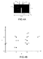
- the experimental setup ( Figure 4A ) is substantially that of the Figure 1A with a laser diode 8 of emission wavelength at about 635 nm (H & B laser diode) as the excitation source and a photomultiplier 4 coupled to a TCSPC card.
- optical properties are identical to the excitation wavelength and the emission wavelength, because of the proximity of the wavelengths of excitation and diffusion, sufficient for consider these coefficients constant over this wavelength range.
- the fluorescent medium in question is Cy5 of concentration 10 .mu.mol.
- the lifetime ⁇ is 0.96 ns, and the refractive index n 0 of the medium is 1.33.
- the Figure 4A shows in more detail the positioning of the sample in the tank 21.
- the latter is placed in a glass capillary tube 23, of internal diameter 1 mm, over a height of about 2 mm.
- This figure also shows the portion of the fibers 10 and 12 which are immersed in the examined medium.
- the end of each fiber is located 3.5 cm below the level of the liquid, which is sufficient to ensure the condition of infinite medium.
- the power measured at the output of the excitation fiber 10 is 100 ⁇ W.
- the detector is in position Di.
- the figure 4C gives the fluorescence curve obtained for each pair of positions (Si, Di). The curves were previously processed as explained in A.Laidevant et al., Applied Optics, 45, 19, 4756 (2006) ).
- intersection of these three surfaces has also been calculated.
- the Figures 4D and 4E represent in each of the planes XY and ZY (respectively respectively in top view and side view of the tank 21) the measured position p 1 and the calculated position P 0 , with a slight shift between these two positions.
- the figure 4F represents these two positions in three dimensions, with, also, a slight difference between these two positions. Despite this discrepancy, it is found that the information obtained by the calculation is quite satisfactory for a good number of cases, for example for an approximate location in an organ of the human body.
- the total computation time with standard computer hardware is quite compatible with a measurement on or in an organ of the human body, for example during a surgical procedure or in a unit of analysis.
- This example is in three dimensions, and in semi-infinite medium.
- optical properties are the same as in the previous example.
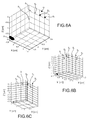
- Zone I The intersection zone of these 3 ellipsoids is identified by zone I in Figure 6A , on which are further represented the three positions S1, S2, S3 of the source and the three positions D1, D2, D3 of the detector used for the three measurements.
- Zone P is the localization area of the fluorophore.
- the solution of the Figure 6A is an approximate solution, within 10%.
- a practitioner may perform an analysis according to the invention even though it is in the presence of a patient.
- a duration of 10 seconds, or even a slightly longer duration, is entirely compatible with keeping a patient on an operating table or in an analysis room.
- the third corresponds to a measurement whose optical path is the shortest of the three. It is this measure which, as explained in the application EP 1 884 765 , can be used as a reference measure.
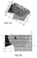
- FIGS 7A and 7B represent, in two different orientations, the intersection between the two 3D surfaces ⁇ 1 - ⁇ 3 (zone I in these figures) and ⁇ 2 - ⁇ 3 (zone II in these figures).
- a third surface is needed to identify a possible location of the fluorophore.
- r s1 [0.0, 0, 0]
- r s2 [0.5, 0, 0]
- r s3 [0.75, - 1, 0]
- r s4 [-0.75; -1.5; 0];
- This surface ⁇ 4 will also be normalized. We thus make the difference ⁇ 4 - ⁇ 3 which defines itself a surface whose intersection with the surfaces ⁇ 1 - ⁇ 3 and ⁇ 2 - ⁇ 3 will allow to locate the fluorophore.
- the Figure 7C represents the 3 surfaces ⁇ 1 - ⁇ 3 , (zone I), ⁇ 2 - ⁇ 3 (zone II) and ⁇ 4 - ⁇ 3 (zone III), while the Figure 7D represents a section of the set in an XZ plane.
- zone P The zone of intersection of the 3 surfaces, and therefore the zone of localization of the fluorophore, is identified by the zone P on this Figure 7D .
- This example is in three dimensions, and in "slab" type geometry.
- zone I in figure 8D The intersection zone of these 3 ellipsoids is identified by zone I in figure 8D , on which are furthermore represented the three positions of the source and the three positions of the detector used for the three measurements.
- an exemplary method according to the invention can be implemented according to the diagram represented in FIG. figure 9 .
- a fluorophore or absorber intended to be fixed on an area of interest.
- a fluorophore when injected, many are often injected.
- concentration when working in absorption, there is not only one absorbing molecule, but a concentration of absorbing molecules. This concentration can be considered as point if the distance separating it from the detector is sufficiently large in front of its dimensions.
- a concentration of radius r is considered as point, at a given observation distance d, if d> 10 r.
- Some absorbers may already be in the medium, for example when it is a zone with a different absorption of its environment.
- the radiation emission and detection means are then positioned relative to the medium.
- One of the configurations already described can be selected.
- a non-invasive invasive examination can be performed.
- a first step S1 of this method input data or parameters are provided: these are the optical properties of the scattering medium, at the two wavelengths of excitation and emission (in some cases, at these two wavelengths, the optical properties are identical), the geometry of the medium, the positions of the sources and the detector (in the sense already explained above), and the choice of the mesh for the calculation of the surfaces.
- the measurement files (TPSF) for each source-detector pair are read. Preprocessing of the data can be done.
- an analytic expression of each surface will be able to be determined or calculated for each point of the mesh (step S3).
- step S2 The data from step S2 will allow a calculation of mean times ⁇ t i > for each of the measurements made (step S4).
- Steps S1 and S3 on the one hand, S2 and S34 on the other hand, are represented in figure 9 as substantially performed simultaneously, but it is not necessary, although desirable for the fastest possible process.
- the user can himself set the desired X precision.
- the results (the intersection of the surfaces between it, and possibly each of the surfaces individually) can then be viewed (step S6).
- step S7 the calculations can be reiterated by setting a value of X higher (in which case the precision is reduced) or lower (in which case the precision is increased) to the previous value (step S7).
Landscapes
- Health & Medical Sciences (AREA)
- Life Sciences & Earth Sciences (AREA)
- Biomedical Technology (AREA)
- Heart & Thoracic Surgery (AREA)
- Radiology & Medical Imaging (AREA)
- Biophysics (AREA)
- Pathology (AREA)
- Engineering & Computer Science (AREA)
- Nuclear Medicine, Radiotherapy & Molecular Imaging (AREA)
- Physics & Mathematics (AREA)
- Medical Informatics (AREA)
- Molecular Biology (AREA)
- Surgery (AREA)
- Animal Behavior & Ethology (AREA)
- General Health & Medical Sciences (AREA)
- Public Health (AREA)
- Veterinary Medicine (AREA)
- Investigating, Analyzing Materials By Fluorescence Or Luminescence (AREA)
Description
L'invention concerne le domaine de l'imagerie optique diffuse sur les tissus biologiques par des méthodes résolues en temps.The invention relates to the field of diffuse optical imaging on biological tissues by time-resolved methods.
Elle s'applique à la localisation de fluorophores ou d'absorbeurs dans un milieu diffusant tel que, par exemple, un organe d'un animal ou d'un être humain (cerveau, sein, tout organe où des fluorophores peuvent être injectés).It applies to the localization of fluorophores or absorbers in a diffusing medium such as, for example, an organ of an animal or a human being (brain, breast, any organ where fluorophores can be injected).
En particulier, un intérêt d'une molécule qui absorbe est le suivant. Certaines tumeurs cancéreuses sont visibles par le simple fait qu'elles présentent un coefficient d'atténuation plus important que les tissus sains. Dans ce cas, il est important de pouvoir identifier ces tumeurs.In particular, an interest of a molecule that absorbs is as follows. Some cancerous tumors are visible by the fact that they have a greater attenuation coefficient than healthy tissues. In this case, it is important to be able to identify these tumors.
Dans ce contexte, on peut également être amené à utiliser un fluorophore, qui est un marqueur fluorescent spécifique. Celui-ci vient se fixer de façon préférentielle sur les cellules cibles d'intérêt (par exemple des cellules cancéreuses). Un tel fluorophore offre un meilleur contraste de détection qu'un marqueur non spécifique. Les techniques optiques d'imagerie moléculaire de fluorescence ont pour but de localiser spatialement ces marqueurs fluorescents.In this context, it may also be necessary to use a fluorophore, which is a specific fluorescent marker. It is preferentially attached to the target cells of interest (for example cancer cells). Such a fluorophore offers a better contrast of detection than a non-specific marker. Fluorescence molecular imaging optical techniques are aimed at spatially locating these fluorescent markers.
Les systèmes de tomographie optique utilisent diverses sources de lumière. Il existe donc des appareils qui fonctionnent en mode continu, d'autres en mode fréquentiel (qui utilisent des lasers modulés en fréquence) et enfin des appareils fonctionnant en mode temporel, qui utilisent des lasers pulsés.Optical tomography systems use a variety of light sources. There is therefore devices that operate in continuous mode, others in frequency mode (which use frequency modulated lasers) and finally devices operating in time mode, which use pulsed lasers.
Ainsi, il existe trois méthodes d'imagerie optique diffuse, qui se distinguent selon que la source de lumière utilisée soit continue, fréquentielle (i.e. dont l'intensité est modulée par une fonction sinusoïde du temps) ou pulsée.Thus, there are three methods of diffuse optical imaging, which differ depending on whether the light source used is continuous, frequency (i.e. whose intensity is modulated by a sinusoidal function of time) or pulsed.
Les instruments utilisant une source de lumière continue ont été les premiers à être utilisés, la source de lumière étant une source blanche filtrée ou une source monochromatique, telle un Laser. On utilise alors des détecteurs ponctuels ou bidimensionnels mesurant l'intensité de la lumière réfléchie ou transmise par un tissu éclairé par la source lumineuse.Instruments using a continuous light source were the first to be used, the light source being a filtered white source or a monochromatic source, such as a laser. Point or two-dimensional detectors are then used, measuring the intensity of the light reflected or transmitted by a fabric illuminated by the light source.
La seconde catégorie d'imagerie optique diffuse, dite imagerie fréquentielle, utilise une source de lumière modulée en intensité à une fréquence donnée. La source lumineuse est le plus souvent une source laser modulée en intensité à des fréquences f généralement comprises entre quelques dizaines de kHz à quelques centaines de MHz. Le détecteur utilisé mesure à la fois l'amplitude du signal lumineux réfléchi ou transmis par le tissu, ainsi que la phase de ce signal lumineux par rapport à celle de la source de lumière.The second category of diffuse optical imaging, called frequency imaging, uses a light source modulated in intensity at a given frequency. The light source is most often a laser source intensity modulated at frequencies f generally between a few tens of kHz to a few hundred MHz. The detector used measures both the amplitude of the light signal reflected or transmitted by the tissue, as well as the phase of this light signal relative to that of the light source.
Enfin, la troisième catégorie d'imagerie optique diffuse est l'imagerie optique diffuse pulsée, également appelée imagerie optique diffuse impulsionelle, ou encore temporelle, ou encore résolue en temps. La source utilisée produit des impulsions lumineuses dites impulsionnelles, c'est-à-dire de courte durée, à un taux de répétition donné. Les sources utilisées peuvent être des diodes laser pulsées picosecondes, ou des lasers femtosecondes. La durée de l'impulsion étant généralement inférieure à 1ns, on parlera alors de sources lumineuses pulsées subnanosecondes. Le taux de répétition est le plus souvent compris entre quelques centaines de kHz à quelques centaines de MHz.Finally, the third category of diffuse optical imaging is pulsed optical diffuse imaging, also known as diffuse optical imaging. impulse, or temporal, or resolved in time. The source used produces pulses of pulses, that is to say of short duration, at a given repetition rate. The sources used may be pulsed picosecond laser diodes, or femtosecond lasers. The duration of the pulse being generally less than 1ns, then we speak of subnanosecond pulsed light sources. The repetition rate is most often between a few hundred kHz to a few hundred MHz.
L'invention concerne cette troisième catégorie d'imagerie de fluorescence.The invention relates to this third category of fluorescence imaging.
Document
Les données temporelles sont celles qui contiennent le plus de contenu informationnel sur le tissu traversé, mais pour lesquelles les techniques de reconstruction sont les plus complexes. La mesure en chaque point d'acquisition est en effet une fonction dépendante du temps (appelée TPSF pour « Temporal Point Spread Function », ou fonction d'étalement temporel).Time data is the one that contains the most informational content on the fabric that is traversed, but for which reconstruction techniques are the most complex. The measurement at each acquisition point is indeed a time dependent function (called TPSF for "Temporal Point Spread Function", or time spreading function).
On cherche à extraire des paramètres simples de la TPSF, dont on connaît par ailleurs l'expression théorique. Ensuite, la résolution du problème inverse permet de retrouver la distribution des marqueurs fluorescents.It seeks to extract simple parameters of the TPSF, which is also known theoretical expression. Then, the resolution of the inverse problem makes it possible to find the distribution of the fluorescent markers.
Dans certains cas, on cherche à localiser un fluorophore en vue d'une intervention ultérieure. A l'heure actuelle, la localisation de cellules malades peut se faire à l'aide des techniques de biopsie. Mais, afin de trouver la position, même approximative, de ces cellules, on doit effectuer plusieurs prélèvements. Cette technique invasive est évidemment délicate à mettre en oeuvre et est consommatrice de temps.In some cases, it is sought to locate a fluorophore for later intervention. At present, the location of diseased cells can be done using biopsy techniques. But, in order to find the position, even approximate, of these cells, one must make several samples. This invasive technique is obviously difficult to implement and is time consuming.
Il se pose donc le problème de la détermination de la localisation, même de manière approximative, d'un fluorophore ou d'un absorbeur fixé sur une zone d'un milieu, par exemple un milieu biologique, cela avec un nombre limité de mesures, et une durée de dépouillement relativement faible, voire proche du temps réel. L'invention trouve toute son utilité pour réaliser une telle détermination dans des milieux présentant une accessibilité limitée, par exemple lors du dépistage de tumeurs cancéreuses de la prostate à partir de mesures endoscopiques, ou lors du dépistage de cancers du sein, ou d'ostéosarchomes....There is therefore the problem of determining the location, even approximately, of a fluorophore or an absorber fixed on an area of a medium, for example a biological medium, with a limited number of measurements, and a relatively low stripping time, even close to real time. The invention finds all its utility for making such a determination in media with limited accessibility, for example when screening for prostate cancer tumors from endoscopic measurements, or when screening for breast cancer, or osteosarchomia ....
L'invention concerne d'abord un procédé de localisation d'au moins un fluorophore ou d'au moins un élément (molécule notamment) absorbant - encore appelé absorbeur - dans un milieu diffusant, à l'aide d'une source de rayonnement apte à émettre un rayonnement d'excitation de ce fluorophore et des moyens de détection apte à mesurer :
- un signal de fluorescence (Φfluo) émis par ce fluorophore,
- ou un signal réémis à la même longueur d'onde que celle d'excitation (issue de la source de rayonnement) par l'élément absorbant qui absorbe et diffuse le rayonnement absorbé. L'élément absorbant peut faire partie d'une zone d'un milieu qui présente un coefficient d'absorption supérieur à celui du milieu diffusant. On a déjà donné l'exemple de certaines tumeurs cancéreuses.
- a fluorescence signal (Φ fluo ) emitted by this fluorophore,
- or a signal re-emitted at the same wavelength as that of excitation (from the radiation source) by the absorbing element which absorbs and diffuses the absorbed radiation. The absorbent element may be part of an area of a medium that has an absorption coefficient greater than that of the medium broadcasting. We have already given the example of certain cancerous tumors.
Ce procédé de localisation comporte les étapes suivantes:
- a) pour au moins 3 couples différents de positions de la source de rayonnement et des moyens de détection, au moins une excitation par un rayonnement provenant de la source de rayonnement, et au moins une détection par les moyens de détection du signal de fluorescence émis par ce fluorophore après cette excitation, ou du signal d'émission émis par l'absorbeur ou par l'élément absorbant,
- b) pour chacun de ces couples, l'identification d'une surface sur laquelle le fluorophore (ou l'élément absorbant) est situé, ou d'un volume comprenant cette surface et dans lequel le fluorophore ou l'absorbeur est situé,
- c) une estimation de la localisation du fluorophore ou de la localisation de l'élément absorbant dans son milieu diffusant, par calcul de l'intersection des trois surfaces, ou éventuellement dans un volume autour de cette intersection.
- a) for at least 3 different pairs of positions of the radiation source and detection means, at least one excitation by radiation from the radiation source, and at least one detection by the fluorescence signal detection means by this fluorophore after this excitation, or of the emission signal emitted by the absorber or by the absorbing element,
- (b) for each of these pairs, the identification of a surface on which the fluorophore (or absorbent element) is located, or a volume comprising that surface and in which the fluorophore or absorber is located,
- c) an estimation of the location of the fluorophore or the location of the absorbent element in its scattering medium, by calculating the intersection of the three surfaces, or possibly in a volume around this intersection.
Les signaux peuvent être détectés par exemple par technique TCSPC ou par caméra.The signals can be detected for example by TCSPC technique or by camera.
Un tel procédé peut être mis en oeuvre quelles que soient les positions respectives du fluorophore ou de l'absorbeur, de la source et du détecteur.Such a method can be implemented regardless of the respective positions of the fluorophore or absorber, the source and the detector.
La précision du procédé ne sera pas la même suivant que l'on prend des positions de la source et des moyens de détection rapprochées ou éloignées du fluorophore ou de l'absorbeur. Mais le procédé permet dans tous les cas une localisation, même grossière, avec un faible nombre de mesures, avec un dépouillement rapide, voire en temps réel. Un tel procédé permet donc d'orienter la réalisation de biopsies ou d'examens non invasifs complémentaires.The accuracy of the method will not be the same depending on whether one takes positions of the source and detection means near or far from the fluorophore or absorber. But the process allows in all cases a location, even rough, with a small number of measurements, with a fast stripping, even in real time. Such a method therefore makes it possible to direct the performance of biopsies or complementary non-invasive examinations.
En outre ce procédé est de mise en oeuvre très rapide, on peut réaliser une localisation d'un fluorophore ou d'absorbeur en moins d'une minute, ou même en moins de 15 s.In addition, this method is very quick to implement, it is possible to locate a fluorophore or absorber in less than one minute, or even in less than 15 seconds.
Pour chaque couple des au moins 3 couples différents, on peut définir un histogramme représentant le nombre de photons détectés en fonction du temps ; cet histogramme peut être appelé fonction temporelle de fluorescence.For each pair of at least 3 different pairs, it is possible to define a histogram representing the number of photons detected as a function of time; this histogram can be called the fluorescence time function.
La source de rayonnement ou de lumière et/ou les moyens de détection peuvent être respectivement l'extrémité d'une fibre optique qui amène la lumière d'excitation dans le milieu et/ou l'extrémité d'une fibre optique qui prélève une partie de la lumière d'émission. Pour la source, il peut également s'agir d'une source lumineuse de type Laser ou LED. En ce qui concerne le détecteur, il peut s'agir d'un tube photomultiplicateur, ou d'un capteur d'image.The source of radiation or light and / or the detection means may be respectively the end of an optical fiber which brings the excitation light into the medium and / or the end of an optical fiber which takes a part emission light. For the source, it can also be a light source of the Laser or LED type. Regarding the detector, it may be a photomultiplier tube, or an image sensor.
Selon l'invention l'élément visé par la détection peut être un fluorophore unique, ou une pluralité ou une agrégation de fluorophores groupés sensiblement en un même lieu. Il peut également s'agir d'un absorbeur ou d'une pluralité d'absorbeurs groupés sensiblement en un même lieu (agrégation). Dans la suite du texte, un absorbeur sera assimilé à un fluorophore dont la longueur d'onde d'émission est égale à la longueur d'onde d'excitation, et dont la durée de vie est nulle. Autrement dit un milieu absorbant, ou un absorbeur, est un fluorophore dont la longueur d'onde d'émission est égale à la longueur d'onde d'excitation, et dont la constante de temps τ est nulle. On n'emploiera donc que l'expression « fluorophore », sauf lorsque des spécificités des absorbeurs sont expliquées.According to the invention the element targeted by the detection may be a single fluorophore, or a plurality or an aggregation of fluorophores grouped substantially in one place. It can also be an absorber or a plurality of absorbers grouped substantially in one place (aggregation). In the rest of the text, an absorber will be assimilated to a fluorophore whose emission wavelength is equal to the excitation wavelength, and whose lifetime is zero. In other words, an absorbing medium, or an absorber, is a fluorophore whose emission wavelength is equal to the excitation wavelength, and whose time constant τ is zero. Only the term "fluorophore" will be used, except when specificities of the absorbers are explained.
Le volume autour de l'intersection des trois surface calculées peut résulter de l'intersection de trois volumes, chaque volume étant associé à l'une des surfaces et comportant l'ensemble des points de la surface et l'ensemble des points qui satisfont à l'équation de la surface avec une marge d'erreur, par exemple ± 10% ou ± 5%.The volume around the intersection of the three calculated surfaces can result from the intersection of three volumes, each volume being associated with one of the surfaces and comprising all the points of the surface and all the points which satisfy the surface equation with a margin of error, for example ± 10% or ± 5%.
Le milieu diffusant environnant le fluorophore peut avoir toute forme de géométrie : par exemple, il est de type infini.The diffusing medium surrounding the fluorophore may have any shape of geometry: for example, it is of infinite type.
Il peut aussi être de type semi-infini, limité par une paroi. Un milieu semi infini, pour lequel chacune des extrémités de fibres d'amenée du signal d'excitation et de prélèvement du signal de fluorescence est disposée à plus de 1 cm, ou de 1,5 cm ou de 2 cm de la paroi qui limite ce milieu peut être traité, du point de vue du procédé selon l'invention, comme un milieu infini.It can also be of semi-infinite type, limited by a wall. A semi-infinite medium, for which each of the fiber ends of the excitation signal and the fluorescence signal collection signal is disposed more than 1 cm, or 1.5 cm or 2 cm from the limiting wall. this medium can be treated, from the point of view of the process according to the invention, as an infinite medium.
Le milieu diffusant peut encore former une tranche (géométrie dite « slab »), limitée par deux surface parallèles. L'invention s'applique aussi à un milieu de forme quelconque, dont la surface extérieure est décomposée en une série de plans.The diffusing medium can still form a slab (geometry called "slab"), limited by two parallel surfaces. The invention also applies to a medium of any shape, the outer surface of which is decomposed into a series of planes.
Dans certains modes de réalisation, les surfaces à l'intersection desquelles se trouve le fluorophore, peuvent avoir la forme d'ellipsoïdes, mais il peut également s'agir de surfaces 3D n'ayant pas cette forme.In some embodiments, the surfaces at the intersection of which the fluorophore is located may be in the form of ellipsoids, but may also be 3D surfaces not having this shape.
Selon un mode de réalisation, l'étape b) comporte pour chaque couple de position, un calcul d'un moment temporel normé, d'ordre n (n≥ 1), d'une fonction temporelle de fluorescence. Un tel moment peut être obtenu par une dérivée d'ordre n d'une transformée de ladite fonction temporelle de fluorescence, par exemple une transformée de Fourier, ou une transformée de Laplace ou une transformée de Mellin.According to one embodiment, step b) comprises, for each position pair, a calculation of a normed time moment, of order n (
On rappelle qu'un moment normé d'ordre n (n≥ 1), noté mn d'une distribution g(t) est défini par 
Dans certains cas, il peut être avantageux de réaliser une excitation par une source de lumière, et une détection par les moyens de détection, pour 4 couples différents de positions de la source de rayonnement et des moyens de détection.In some cases, it may be advantageous to carry out excitation by a light source, and detection by the detection means, for 4 different pairs of positions of the radiation source and detection means.
On peut ensuite :
- sélectionner parmi les quatre couples, le couple de points, dit quatrième couple de points, pour lequel la durée moyenne d'arrivée des photons, de l'émetteur au récepteur, est la plus courte, et calculer, pour ce quatrième couple de points, l'équation d'une surface sur laquelle le fluorophore est situé ;
- et, pour chacun des trois autres couples de points, après calcul d'une première équation d'une surface sur laquelle le fluorophore est situé, on peut effectuer une différence entre cette équation et celle associée au quatrième couple, pour obtenir une deuxième équation indépendante de la durée de vie du fluorophore.
- selecting from the four pairs, the pair of points, said fourth pair of points, for which the average duration of arrival of the photons, from the transmitter to the receiver, is the shortest, and calculate, for this fourth pair of points, the equation of a surface on which the fluorophore is located;
- and, for each of the other three pairs of points, after calculating a first equation of a surface on which the fluorophore is located, a difference can be made between this equation and that associated with the fourth pair, to obtain a second independent equation the life of the fluorophore.
On peut donc, selon un mode de réalisation, lors de l'étape b) pour chaque couple de position, calculer une équation de chaque surface, indépendante de la durée de vie du fluorophore, qui peut résulter de la différence entre le temps moyen calculé pour chaque couple de position et le temps moyen calculé pour un autre couple de position. Cet autre couple de position peut être celui ayant un temps moyen minimal ou ayant un temps moyen calculé minimal.According to one embodiment, it is therefore possible, during step b) for each pair of positions, to calculate an equation of each surface, independent of the lifetime of the fluorophore, which can result from the difference between the calculated average time for each position torque and the calculated average time for another position torque. This other pair of positions can be the one having a minimum average time or having a minimum calculated average time.
Un procédé selon l'invention peut en outre comporter une représentation visuelle ou graphique de la position ou de la répartition du ou des fluorophores ou absorbeurs.A method according to the invention may further comprise a visual or graphical representation of the position or distribution of the fluorophore or absorbers.
L'invention concerne également un procédé pour localiser une zone dans un milieu, comportant l'introduction dans ce milieu d'au moins un fluorophore ou d'un absorbeur, et la localisation de ce fluorophore ou de cet absorbeur dans ledit milieu par un procédé selon l'invention. La zone peut être par exemple un milieu constitué d'un organe humain ou animal, le fluorophore ou l'absorbeur permettant de marquer cette zone. Le but peut être de localiser des cellules malades dans un tel milieu. Comme déjà indiqué ci-dessus, l'invention permet de réaliser cette localisation en un temps rapide, ou même en temps réel.The invention also relates to a method for locating an area in a medium, comprising introducing into this medium at least one fluorophore or an absorber, and the localization of this fluorophore or absorber in said medium by a method according to the invention. The zone may be for example a medium consisting of a human or animal organ, the fluorophore or absorber for marking this zoned. The goal may be to locate diseased cells in such a medium. As already indicated above, the invention makes it possible to achieve this location in a fast time, or even in real time.
Un procédé selon l'invention peut être mis en oeuvre de manière invasive ou non invasive.A method according to the invention can be implemented invasively or non-invasively.
L'invention concerne également un dispositif pour mettre en oeuvre un procédé selon l'invention, et permettant la localisation d'un fluorophore dans un milieu diffusant.The invention also relates to a device for implementing a method according to the invention, and for locating a fluorophore in a diffusing medium.
L'invention concerne donc également un dispositif pour la localisation d'un fluorophore dans un milieu diffusant, qui peut être de l'un des types évoqués plus haut, comportant :
- au moins une source de lumière ou de rayonnement, apte à émettre un rayonnement d'excitation de ce fluorophore,
- au moins un moyen de détection apte à mesurer un signal de fluorescence (Φfluo) émis par ce fluorophore,
- des moyens de calcul, programmés pour calculer :
- a) pour chaque couple de points parmi au moins 3 couples différents de positions d'une source de rayonnement et d'un moyen de détection, la détermination, après une excitation réalisée par un rayonnement provenant de la source de rayonnement, et une détection par les moyens de détection des signaux de fluorescence émis par ce fluorophore après cette excitation, d'une surface sur laquelle le fluorophore est situé, ou un volume comprenant cette surface et dans lequel le fluorophore est situé,
- b) une estimation de la localisation du fluorophore dans son milieu environnant, par calcul de l'intersection des trois surfaces ou d'un volume autour de cette intersection.
- at least one light or radiation source capable of emitting excitation radiation from this fluorophore,
- at least one detection means capable of measuring a fluorescence signal (Φ fluo ) emitted by this fluorophore,
- calculating means, programmed to calculate:
- a) for each pair of points among at least 3 different pairs of positions of a radiation source and detection means, the determination, after an excitation performed by radiation from the radiation source, and a detection by the means for detecting the fluorescence signals emitted by this fluorophore after this excitation, of a surface on which the fluorophore is located, or a volume comprising this surface and in which the fluorophore is located,
- b) an estimate of the location of the fluorophore in its surrounding environment, by calculating the intersection of the three surfaces or a volume around this intersection.
Le milieu environnant peut être de type infini ou de type semi-infini ou en forme une tranche, limitée par deux surfaces parallèles, ou de forme quelconque, sa surface extérieure étant décomposée en une série de plans.The surrounding medium may be of infinite type or semi-infinite type or shaped slice, limited by two parallel surfaces, or any shape, its outer surface being decomposed into a series of planes.
Les moyens de calcul, par exemple des moyens électroniques tels qu'un micro ordinateur ou un calculateur ou un microprocesseur, sont programmés pour mémoriser et traiter des données de fluorescence ou d'émission obtenues des moyens de détection. De préférence ces moyens sont programmés pour mettre en oeuvre un procédé de traitement selon l'invention.The calculation means, for example electronic means such as a microcomputer or a computer or a microprocessor, are programmed to store and process fluorescence or emission data obtained from the detection means. Preferably these means are programmed to implement a treatment method according to the invention.
Les moyens de calcul permettent de calculer, pour chaque couple de position, un moment temporel normé, d'ordre n (n≥ 1), d'une fonction temporelle de fluorescence. Ce moment peut être obtenu à partir d'une fonction fréquentielle, déduite de ladite fonction temporelle de fluorescence par exemple par transformée de Fourier ou par transformée de Mellin.The calculation means make it possible to calculate, for each position pair, a normed time moment, of order n (
Selon un mode avantageux, les moyens de calcul permettent ou sont programmés pour réaliser, pour la localisation d'au moins un fluorophore ou absorbeur, et pour chaque couple de position, un calcul d'une équation de chaque surface, indépendante de la durée de vie du fluorophore. A cette fin, les moyens de calcul permettent de réaliser la différence entre le temps moyen calculé pour chaque couple de position et le temps moyen mesuré ou calculé pour un autre couple de position.According to an advantageous embodiment, the calculation means allow or are programmed to perform, for the localization of at least one fluorophore or absorber, and for each position pair, a calculation of an equation of each surface, independent of the lifetime of the fluorophore. For this purpose, the calculation means make it possible to make the difference between the average time calculated for each position torque and the average time measured or calculated for another position torque.
Le dispositif permet une excitation par la source de rayonnement, et une détection par les moyens de détection pour 4 couples différents de positions de la source de rayonnement et des moyens de détection.The device allows excitation by the radiation source, and detection by the detection means for 4 different pairs of positions of the radiation source and detection means.
Le quatrième couple de position peut être un couple pour lequel le signal de fluorescence a un temps moyen mesuré ou un temps moyen calculé inférieur à celui des 3 couples de position.The fourth position torque may be a pair for which the fluorescence signal has a measured average time or a calculated average time less than that of the 3 position pairs.
-
Les
figures 1A et 1B représentent chacune un exemple de dispositif expérimental pour la mise en oeuvre de l'invention,TheFigures 1A and 1B each represent an example of an experimental device for implementing the invention, -
les
figures 2A et 2B représentent respectivement une série d'impulsions laser et de photons uniques émis, et une courbe de fluorescence obtenue à partir des données relatives aux photons uniques,theFigures 2A and 2B represent respectively a series of laser pulses and single emitted photons, and a fluorescence curve obtained from the data relating to single photons, -
la
figure 3 représente une configuration théorique, en deux dimensions,thefigure 3 represents a theoretical configuration, in two dimensions, -
les
figures 4A-4F représentent le dispositif expérimental d'une mesure réalisée, le positionnement des points source et de détection, des courbes de fluorescence mesurées, et la position calculée et la position réelle d'un fluorophore;theFigures 4A-4F represent the experimental setup of a realized measurement, the positioning of the source and detection points, the measured fluorescence curves, and the calculated position and actual position of a fluorophore; -
la
figure 5A représente des couples de positions d'une source et d'un détecteur, dans un plan XY, en vue d'une mesure selon l'invention, en configuration semi-infinie,theFigure 5A represents pairs of positions of a source and a detector, in an XY plane, for a measurement according to the invention, in semi-infinite configuration, -
les
figures 5B-5D représentent des portions d'ellipsoïdes utilisés dans la cadre d'une mesure selon l'invention, en configuration semi-infinie,theFigures 5B-5D represent portions of ellipsoids used in the context of a measurement according to the invention, in semi-infinite configuration, -
les
figures 6A-6C représentent chacune une localisation d'un fluorophore obtenue avec un procédé selon l'invention, en configuration semi-infinie,theFigures 6A-6C each represent a localization of a fluorophore obtained with a process according to the invention, in a semi-infinite configuration, -
les
figures 7A - 7D représentent des surfaces mises en oeuvre dans le cadre d'un autre mode de réalisation de l'invention,theFigures 7A - 7D represent surfaces used in the context of another embodiment of the invention, -
les
figures 8A-8D représentent des portions de surfaces utilisées dans la cadre d'une mesure selon l'invention, en configuration de tranche.theFigures 8A-8D represent portions of surfaces used in the context of a measurement according to the invention, in slice configuration. -
la
figure 9 représente un schéma de déroulement d'un procédé selon l'invention.thefigure 9 represents a flow diagram of a method according to the invention. -
les
figures 10A-10D représentent diverses dispositions, par rapport à un milieu étudié, de moyens d'excitation et de détection, ou de fibres optiques amenant à ce milieu un rayonnement d'excitation et transmettant un rayonnement à détecter.theFigures 10A-10D represent various arrangements, with respect to a medium studied, excitation and detection means, or optical fibers leading to this medium excitation radiation and transmitting a radiation to be detected.
La
Le dispositif de la
La lumière est émise par une source 8 de rayonnement en impulsions. La durée de chaque impulsion est généralement inférieure à 1ns, par exemple comprise entre d'une part quelques centaines de fs, par exemple 500 fs, ou 100 ps ou 500 ps et d'autre part 100 ps ou 500 ps ou 1 ns. Le taux de répétition est de préférence compris entre quelques centaines de kHz, par exemple 100 kHz ou 500 kHz et quelques centaines de MHz, par exemple 100 MHz ou 500 MHz.The light is emitted by a
La lumière émise par la source 8 est envoyée et collectée par des fibres 10, 12 qui peuvent être déplacées. Les deux fibres peuvent être montées sur des moyens de déplacement en translation verticaux et horizontaux (suivant les axes X, Y et Z de la
La source 8 d'impulsions de rayonnement peut également être utilisée comme moyen de déclenchement de la carte TCSPC (voir la liaison 9 entre la source 8 et les moyens 24). Il est également possible de travailler avec des impulsions dans le domaine de la femto seconde, à condition de disposer de la source de rayonnement adéquate, c'est-à-dire d'une source laser 8 dont chaque impulsion a une largeur temporelle également dans le domaine de la femto seconde.The
Selon un mode particulier de réalisation, la source 8 est une diode laser pulsée, par exemple à une longueur d'onde voisine de 630 nm et avec un taux de répétition d'environ 50 MHz.According to a particular embodiment, the
La lumière laser passe de préférence par un filtre interférentiel 14 pour éliminer d'éventuels modes secondaires.The laser light preferably passes through an
La fibre 12 collecte la lumière en provenance du milieu 20 étudié, en particulier la lumière diffusée par ce milieu. Un filtre interférentiel 16 et/ou un filtre coloré absorbant les faibles longueurs d'onde peuvent être placés devant le détecteur 4 pour sélectionner la lumière de fluorescence (par exemple : λ > 650 nm, la source étant à une longueur d'onde de, par exemple, 631 nm) d'un fluorophore 22 disposé dans le milieu 20 et optimiser l'élimination de la lumière d'excitation.The
Dans le texte de la présente demande, quel que soit le mode de réalisation de l'invention, il sera notamment question de la position de la source de rayonnement, et/ou de la position des moyens de détection. Lorsque des fibres sont utilisées, ces positions s'entendent le plus souvent comme celles des extrémités des fibres qui amènent le rayonnement dans le milieu diffusant 20, ou à l'interface de ce milieu, et /ou celles qui collectent le rayonnement diffusé, ces dernières étant placées dans le milieu ou à l'interface de ce milieu, mais ne s'entendent alors pas comme étant celles de la source 8 proprement dite ou du détecteur 4 proprement dit.In the text of the present application, whatever the embodiment of the invention, it will include question of the position of the radiation source, and / or the position of the detection means. When fibers are used, these positions are most often understood as those of the ends of the fibers which bring the radiation into the diffusing
En variante, on peut utiliser une source de lumière délivrant un faisceau lumineux, par exemple un laser en émission, et une caméra munie d'un objectif en sortie, ce qui permet un couplage optique entre la face sensible de la caméra et la face de sortie de l'objet observé (ce qui est le cas du dispositif de la
En application de type « endoscopie », on utilise préférentiellement un système à fibres, les fibres pouvant être par exemple intégrées dans une sonde endo-rectale, au moins une fibre transmettant la source de lumière pulsée d'excitation à la zone à examiner. Cette source de lumière pulsée peut être externe à la sonde. Au moins une autre fibre transmet le signal optique d'émission de la zone à examiner vers un photodétecteur, qui peut lui aussi être externe à la sonde. Selon la technique TCSPC (pour « Time Correlated Single Photon Counting », ou comptage de photons uniques correlés en temps) on détecte, à l'aide du photomultiplicateur, un photon émis par le fluorophore après une impulsion de la source de rayonnement.In "endoscopic" type application, a fiber system is preferably used, the fibers being able for example to be integrated in an endo-rectal probe, at least one fiber transmitting the pulsed excitation light source to the zone to be examined. This pulsed light source may be external to the probe. At least one other fiber transmits the optical transmission signal of the area to be examined to a photodetector, which may also be external to the probe. According to the TCSPC (Time Correlated Single Photon Counting) technique, a photon emitted by the fluorophore is detected by means of the photomultiplier after a pulse of the radiation source.
Le système permet donc une détection résolue en temps des impulsions de fluorescence. Il permet de récupérer des photons de fluorescence.The system therefore allows time-resolved detection of the fluorescence pulses. It allows to recover fluorescence photons.
La
Il est donc ensuite possible d'établir une répartition statistique ou histogramme du temps d'arrivée des photons, comme illustré sur la
Une telle courbe Φfluo (t) qui, on le voit (voir également l'exemple de la
Des moyens électroniques 24 tels qu'un micro ordinateur ou un calculateur sont programmés pour mémoriser et traiter les données de la carte TCSPC. Plus précisément une unité centrale 26 est programmée pour mettre en oeuvre un procédé de traitement selon l'invention. Des moyens 27 d'affichage ou de visualisation permettent, après traitement, de représenter le positionnement du ou des fluorophores dans le milieu 20 examiné.Electronic means 24 such as a microcomputer or a computer are programmed to store and process the data of the TCSPC card. More specifically, a
D'autres techniques de détection peuvent être employées, par exemple avec une caméra intensifiée, et par exemple une caméra intensifiée ultra-rapide de type « gated camera » ; dans ce cas la caméra s'ouvre sur une porte temporelle, de largeur par exemple environ 200 ps, puis cette porte est décalée, par exemple de 25 ps en 25 ps.Other detection techniques may be employed, for example with an intensified camera, and for example a high-speed intensified camera of the "gated camera" type; in this case the camera opens on a time gate, of width for example about 200 ps, then this door is shifted, for example 25 ps in 25 ps.
La
Un faisceau 30 d'excitation de la fluorescence d'un milieu 20, contenant un ou plusieurs fluorophores 22, est émis par une source 37 de rayonnement (non représentée sur la figure) qui peut être du même type que celle présentée ci-dessus en liaison avec la
La distance entre le faisceau lumineux émis par la source, et le détecteur, ou la partie du milieu optiquement couplée au détecteur, est par exemple comprise entre quelques mm et quelques cm, par exemple entre 1 mm et 20 cm dans le cas de milieux biologiques. C'est le cas notamment dans le cas d'une intégration dans une sonde endo-rectale. Le positionnement relatif de la source et du détecteur par rapport à un organe à examiner peut être déterminé par des moyens de type optique ou ultrasonore, par exemple une sonde d'echographie.The distance between the light beam emitted by the source, and the detector, or the part of the medium optically coupled to the detector, is for example between a few mm and a few cm, for example between 1 mm and 20 cm in the case of biological media. . This is particularly the case in the case of integration into an endo-rectal probe. The relative positioning of the source and the detector with respect to an organ to be examined can be determined by means of the optical or ultrasonic type, for example a ultrasound probe.
En variante des dispositifs ci dessus, on peut placer un nombre n de sources lumineuses et un nombre p de détecteurs, avec par exemple 1≤n≤3 et 1≤p≤3, les sources lumineuses et les détecteurs pouvant être des extrémités de fibres optiques reliées respectivement à au moins une source de lumière pulsée ou au moins un photodétecteur, de type photomultiplicateur ou caméra. On combine alors ces positions de manière à avoir au moins 3 couples distincts de positions de la source et de positions de détecteur :
- une position de source S1 (cas n = 1)
successivement avec 3 positions distinctes D1, D2, D3 de détecteur (cas p=3) ; donc on utilise les couples de positions (S1, D1), (S1, D2), (S1, D3), - deux positions distinctes S1 et S2 de la source (cas n = 2)
avec 2ou 3 positions distinctes de détecteur (cas p=2 ou 3) ; donc on utilise par exemple les couples de positions (S1, D1), (S2, D2) et (S1, D2) ou (S1, D1), (S2, D2) et (S1, D3), - trois positions distinctes S1, S2 et S3 de la source (cas n = 3)
avec 1ou 2 positions distinctes de détecteur (cas p=1 ou 2) ; donc on utilise par exemple les couples de positions (S1, D1), (S2, D1) et (S3, D1) ou (S1, D1), (S2, D2) et (S3, D2).
- a source position S1 (case n = 1) successively with 3 distinct detector positions D1, D2, D3 (case p = 3); therefore we use the pairs of positions (S1, D1), (S1, D2), (S1, D3),
- two distinct positions S1 and S2 of the source (case n = 2) with 2 or 3 distinct positions of detector (case p = 2 or 3); therefore, the pairs of positions (S1, D1), (S2, D2) and (S1, D2) or (S1, D1), (S2, D2) and (S1, D3) are used,
- three distinct positions S1, S2 and S3 of the source (case n = 3) with 1 or 2 distinct detector positions (case p = 1 or 2); therefore, the pairs of positions (S1, D1), (S2, D1) and (S3, D1) or (S1, D1), (S2, D2) and (S3, D2) are used, for example.
De préférence on utilise 3 couples pour lesquels les 3 positions de source sont distinctes entre elles et les 3 positions de détecteur sont distinctes entre elles (configuration : (S1, D1), (S2, D2) et (S3, D3)).3 pairs are preferably used for which the 3 source positions are distinct from each other and the 3 detector positions are distinct from each other (configuration: (S1, D1), (S2, D2) and (S3, D3)).
La lumière d'excitation, à la longueur d'onde λx excite le fluorophore qui réémet une lumière dite d'émission à la longueur d'onde λm > λx avec une durée de vie τ. Cette durée de vie correspond à la durée moyenne pendant laquelle les électrons excités restent dans cet état avant de retourner à leur état initial. Les développements qui vont suivre montrent que le cas d'un absorbeur, et donc d'une émission à longueur d'onde sensiblement égale à celle d'excitation avec une durée de vie nulle, peut être déduit de cas d'un fluorophore.The excitation light at the wavelength λ x excites the fluorophore which re-emits a so-called emission light at the wavelength λ m > λ x with a lifetime τ. This lifetime corresponds to the average duration during which the excited electrons remain in this state before returning to their initial state. The following developments show that the case of an absorber, and therefore of a wavelength emission substantially equal to that of excitation with a zero lifetime, can be deduced from the case of a fluorophore.
L'équation de propagation de la lumière d'excitation dans un milieu diffusant produite par la source pulsée de rayonnement s'écrit : ![]()
- rs désigne la position de la source,
- r désigne une position quelconque dans le milieu,
- la fonction Φx(r, t) désigne le débit de fluence du rayonnement d'excitation au point r à l'instant t.
- le coefficient Dx(r) est le coefficient de diffusion au point r, à la longueur d'onde d'excitation λx ;
- Sx(r s, t) désigne le flux de rayonnement émis, à l'instant t, par la source au point rs.
- r s denotes the position of the source,
- r denotes any position in the medium,
- the function Φ x ( r, t) designates the flow rate of the excitation radiation at point r at time t.
- the coefficient D x (r) is the diffusion coefficient at the point r, at the excitation wavelength λ x ;
- S x ( r s , t) denotes the radiation flux emitted at time t by the source at the point r s .
Celle de la lumière d'émission s'écrit : 
avec :
- la fonction Φm(r, t) qui désigne le débit de fluence du rayonnement d'émission au point r, à l'instant t ;
- le coefficient Dm(r), qui est le coefficient de diffusion au point r à la longueur d'onde d'émission λm.
with:
- the function Φ m ( r, t) which designates the fluence rate of the emission radiation at the point r, at time t;
- the coefficient D m (r), which is the diffusion coefficient at the point r at the emission wavelength λm.
Les conditions aux limites étant les suivantes: ![]()
![]()
et ce pour tout point r de la frontière δΩ du milieu diffusant.The boundary conditions being as follows: ![]()
![]()
and this for every point r of the δΩ boundary of the scattering medium.
Ces équations sont aussi développées et expliquées dans la thèse de
Dans ces équations :
- µax et µam sont les coefficients d'absorption du milieu diffusant à la longueur d'onde d'excitation λx et d'émission λm respectivement,
- µax→m est le coefficient d'absorption associé à la concentration locale de fluorophores à la longueur d'onde d'excitation λx;
- η est le rendement quantique du fluorophore,
- Φ(r,t) est le débit de fluence associé à la densité de photons, en photons/m2s, ou, de manière équivalente, en Watt/m2,
- A est égal à (1-Reff)/(1+Reff), où Reff est le coefficient de réflexion dû à la différence d'indice entre l'air et le
milieu 22 environnant le fluorophore.
- μ ax and μ am are the absorption coefficients of the scattering medium at the excitation wavelength λ x and emission λ m respectively,
- μ ax → m is the absorption coefficient associated with the local concentration of fluorophores at the excitation wavelength λ x ;
- η is the quantum yield of the fluorophore,
- Φ (r, t) is the fluence rate associated with the photon density, in photons / m 2 s, or, equivalently, in Watt / m 2 ,
- A is equal to (1-R eff ) / (1 + R eff ), where R eff is the reflection coefficient due to the difference in index between the air and the medium 22 surrounding the fluorophore.
La condition aux limites exprime que, à la frontière du milieu, le débit de fluence diffusé est nul.The boundary condition expresses that, at the middle boundary, the diffused fluence rate is zero.
La fonction théorique Φm peut-être considérée comme proportionnelle à la TPSF, cette dernière étant mesurée expérimentalement (
La résolution du système d'équations couplées obtenu n'est pas aisée, et l'exploitation du volume de données que contient le signal temporel est difficile. On s'intéresse en général à l'exploitation de tel ou tel intervalle de temps extrait de ces fonctions dépendantes du temps (appelées TPSF pour « Temporal Spread Function », ou fonction d'étalement temporel)- pour réaliser une étape d'ajustement ('fitting') avec les données expérimentales.The resolution of the system of coupled equations obtained is not easy, and the exploitation of the volume of data contained in the time signal is difficult. We are generally interested in the exploitation the time interval extracted from these time-dependent functions (called TPSF for "Temporal Spread Function", or time-stretching function) - to perform a fitting step with the experimental data.
Pour exploiter l'information temporelle par le biais d'autres grandeurs, extraites des TPSF mesurées, on peut définir d'autres mesures telles que la mesure des moments - transformées de Mellin de la TPSF, ou des Transformées de Fourier (et donc travailler en mode fréquentiel), ou des Transformées de Laplace ou par paramétrisation de la TPSF (c'est-à-dire la détermination de paramètres caractéristiques tels que les coordonnées du maximum, et/ou le coefficient de pente montante et/ou de pente descendante de la TPSF. L'intérêt de telles grandeurs est de réduire le volume de données en supprimant les éventuelles redondances existant entre ellesTo exploit the temporal information by means of other quantities extracted from the measured TPSF, other measures can be defined such as the measurement of the Mellin transform times of the TPSF, or the Fourier Transforms (and thus to work in frequency mode), or Laplace Transforms or by parameterization of the TPSF (that is to say the determination of characteristic parameters such as the coordinates of the maximum, and / or the coefficient of rising slope and / or downward slope of the interest of such quantities is to reduce the volume of data by removing any redundancies existing between them
Dans la suite de l'invention, on s'intéresse principalement au calcul de moments d'ordre n de l'histogramme, un tel calcul pouvant être réalisé par transformée de Fourier.In the remainder of the invention, the main interest is in calculating n-order moments of the histogram, such a calculation being possible by Fourier transform.
En particulier, on peut, partant de la fonction Φm, en calculer tout moment temporel normé, et notamment le moment d'ordre 1 normé. Une telle grandeur correspond au temps moyen d'arrivée des photons. Les moments temporels normés de la fonction Φm, sont définis comme : 

On va maintenant traiter le cas d'un milieu infini. On peut montrer que le moment temporel normé d'ordre 1 de la fonction Φm, définissant le temps moyen d'arrivée des photons <t>∞, en milieu infini s'écrit : 
où <t>x, <t>m et <t>déclin fluo désignent respectivement la durée moyenne du trajet source-fluorophore, la durée du trajet fluorophore -détecteur, et la durée de vie moyenne de l'espèce excitée (cette dernière étant égale à 0 en présence d'un absorbeur).On rappelle que, en outre :
- rsr = |rs - r|
- rrd = |r-rd|
- m1 est le résultat de la mesure
where <t> x , <t> m and <t> fluo decay are the average duration of the fluorophore source path, the fluorophore-detector trip duration, and the average duration of the excited species (the latter being equal to 0 in the presence of an absorber). It is recalled that, in addition:
- r sr = | r s - r |
- r rd = | rr d |
- m 1 is the result of measurement
On voit qu'on a là l'équation d'une surface 3D, ayant ici la forme d'un ellipsoïde.We see that we have here the equation of a 3D surface, here having the shape of an ellipsoid.
Plus généralement, le moment normé d'ordre k peut s'exprimer sous la forme : 
Où Φ̃(ω) est la transformée de Fourier de Φm: ![]()
Where Φ (ω) is the Fourier transform of Φ m : ![]()
Par exemple, on peut montrer que la variance de la distribution temporelle s'écrit ![]()

![]()
On observe qu'on obtient donc, également dans le cas de la variance, la définition d'une surface tridimensionnelle, ici, celle d'un ellipsoïde.It is observed that we obtain, also in the case of variance, the definition of a three-dimensional surface, here that of an ellipsoid.
Cette grandeur (la variance) peut être calculée dans le cadre de la présente invention à partir des moments d'ordre 2 et 1.This magnitude (the variance) can be calculated in the context of the present invention from moments of
Plus généralement encore on peut, selon l'invention, calculer tout moment d'ordre supérieur à 1, et établir une relation liant au moins un de ces moments aux distances respectives source-fluorophore et fluorophore-détecteur. Si l'on considère des moments d'ordre supérieur, l'équation reliant ces derniers, ou une combinaison de ces derniers, aux distances respectives source-fluorophore et fluorophore-détecteur, est également celle d'une surface tridimensionnelle.More generally still it is possible, according to the invention, to calculate any moment of order greater than 1, and to establish a relationship linking at least one of these moments to the respective distances source-fluorophore and fluorophore-detector. If one considers moments of higher order, the equation connecting them, or a combination of these, to the respective distances source-fluorophore and fluorophore-detector, is also that of a three-dimensional surface.
Préférentiellement, on utilise le moment d'ordre 1 normé.Preferably, the standardized first order moment is used.
D'une manière générale, on peut voir un fluorophore comme capable d'absorber une certaine quantité de lumière (dans son état excité) et d'en réémettre une partie à une longueur d'onde supérieure (lors de sa désexcitation), avec un retard correspondant à la durée dans l'état excité. A partir des expressions données ci dessus on peut donc passer du cas du fluorophore à l'absorbeur simple en écrivant µ ax = µ am , Dx=Dm et τ = 0. Ceci vaut pour tous les cas exposés dans la présente demande. Les considérations ci-dessus valent donc également pour le cas d'un objet absorbant.In general, a fluorophore can be seen to be able to absorb a certain amount of light (in its excited state) and to re-emit a portion of it at a higher wavelength (when it is de-excited), with a delay corresponding to the duration in the excited state. From the expressions given above, it is therefore possible to pass from the case of the fluorophore to the single absorber by writing μ ax = μ am , D x = D m and τ = 0. This applies to all the cases described in the present application. The above considerations therefore also apply to the case of an absorbent object.
Le milieu infini est typiquement celui que l'on rencontre lorsque des mesures invasives sont réalisées, avec des fibres 10, 12 pour amener la lumière dans un milieu 21 (cas de la
On considère une première hypothèse, celle d'un milieu où les propriétés optiques sont identiques aux 2 longueurs d'onde d'excitation et de mesure, λ x et à λm , ce qui est par exemple sensiblement le cas lorsque ces deux longueurs d'onde sont distantes de par exemple de 10 nm ou de quelques dizaines de nm. Rappelons aussi que λx λm lorsqu'on n'a qu'un absorbeur non fluorescent. ; Les propriétés optiques du milieu aux deux longueurs d'ondes peuvent donc être considérées comme identiques. On a alors une simplification de l'équation (7) ci-dessus : ![]()
![]()
Ceci constitue la formule d'un ellipsoïde de foyers S et D, soit le lieu des points r tels que la distance source-fluorophore rsr plus la distance fluorophore-détecteur rrd est égale au produit de la vitesse apparente dans le milieu diffusant ![]()
![]()
Ainsi pour trouver la position 3D du fluorophore, il suffit d'effectuer 3 mesures à trois positions de sources et 3 positions de détecteurs. Le fluorophore est donc à l'intersection de 3 ellipsoïdes définis dans l'espace par 3 équations différentes. De préférence, on sélectionne des couples de positions définissant des directions sensiblement perpendiculaires les unes aux autres. Pour chaque couple, on procède à l'établissement d'une TPSF ou d'un histogramme comme expliqué ci-dessus.Thus, to find the 3D position of the fluorophore, it suffices to perform 3 measurements at 3 source positions and 3 detector positions. The fluorophore is at the intersection of 3 ellipsoids defined in space by 3 different equations. Preferably, couples of positions defining directions substantially perpendicular to each other are selected. For each pair, we proceed to the establishment of a TPSF or a histogram as explained above.
Dans la deuxième hypothèse, le cas où les propriétés optiques ne peuvent pas être considérées identiques aux 2 longueurs d'onde, l'équation (7) devient: 
Ceci est toujours l'équation d'un ellipsoïde mais il traduit maintenant le lieu des points r tels que la distance source-fluorophore rsr soit « pondérée » par la vitesse apparente vx (d'où le terme rsr/vx), et la distance fluorophore-détecteur rrd soit « pondérée » par la vitesse apparente vm (d'où le terme rrd/vm).This is always the equation of an ellipsoid but it now translates the location of the points r such that the source-fluorophore distance r sr is "weighted" by the apparent velocity v x (hence the term r sr / v x ) , and the fluorophore-detector distance r rd is "weighted" by the apparent velocity v m (hence the term r rd / v m ).
Là encore, pour trouver la position 3D du fluorophore, on effectue 3 mesures à trois positions de sources et 3 positions de détecteurs. Le fluorophore est donc à l'intersection de 3 ellipsoïdes définis dans l'espace par 3 équations différentes. De préférence, on sélectionne des couples de positions définissant des directions sensiblement perpendiculaires les unes aux autres. Pour chaque couple de positions (source, détecteur), on procède à l'établissement d'une TPSF ou d'un histogramme comme expliqué ci-dessus. Egalement de préférence, lors de chaque acquisition, on tentera d'augmenter le plus possible la distance source-détecteur.Again, to find the 3D position of the fluorophore, 3 measurements are made at three source positions and 3 detector positions. The fluorophore is at the intersection of 3 ellipsoids defined in space by 3 different equations. Preferably, couples of positions defining directions substantially perpendicular to each other are selected. For each pair of positions (source, detector), one proceeds to the establishment of a TPSF or a histogram as explained above. Also preferably, during each acquisition, we will try to increase as much as possible the source-detector distance.
Les expressions des temps moyens peuvent être données analytiquement pour des géométries autres que celles du milieu infini, plus complexes : milieu semi-infini, avec une interface plane ; milieu plan à faces parallèles...The mean time expressions can be analytically given for geometries other than those of the infinite medium, more complex: semi-infinite medium, with a plane interface; middle plane to parallel faces ...
De manière générale, si l'on connait l'expression, analytique ou numérique, de la transformée de Fourier Φ̃(ω) de la fonction φ m , alors : ![]()
où ![]()
![]()
or ![]()
La surface décrite n'est plus un ellipsoïde, mais reste une surface 3D ; Donc, là encore, on localise un fluorophore par recherche des intersections entre 3 surfaces, chacune obtenue pour un couple de point (position source, position mesure) différent.The described surface is no longer an ellipsoid, but remains a 3D surface; So, again, a fluorophore is located by looking for intersections between 3 surfaces, each obtained for a different point pair (source position, measurement position).
D'une manière générale, dans tous les cas concernés par l'invention (ceux-ci-dessus et les autres exposés ci-dessous), pour trouver la position 3D du fluorophore, on effectue 3 mesures avec trois positions, de préférence différentes entre elles, de sources et 3 positions, de préférence différentes entre elles, de détecteurs (autrement dit, une mesure pour chacun des 3 couples (rsi, rdi), i= 1,2,3, avec rsi ≠ rsj, pour i ≠j et rdi ≠ rdj, pour i ≠j). Le fluorophore est donc à l'intersection de 3 ellipsoïdes définis dans l'espace par 3 équations différentes. De préférence, on sélectionne 3 couples de positions définissant des directions sensiblement perpendiculaires les unes aux autres. Dans certains cas, dont on verra un exemple plus loin, il peut être utile d'effectuer 4 mesures pour 4 couples de positions (source, détecteur). Pour chaque couple de positions (source, détecteur), on procède à l'établissement d'une TPSF ou d'un histogramme comme expliqué ci-dessus.In general, in all the cases concerned by the invention (those above and the others exposed below), to find the 3D position of the fluorophore, three measurements are made with three positions, preferably different between they, from sources and 3 positions, preferably different from each other, detectors (in other words, a measurement for each of the three pairs (r si , r di ), i = 1,2,3, with r si ≠ r sj , for i ≠ j ≠ r and r di dj for i ≠ j). The fluorophore is at the intersection of 3 ellipsoids defined in space by 3 different equations. Preferably, three pairs of positions defining directions substantially perpendicular to each other are selected. In some cases, of which we will see an example later, it may be useful to perform 4 measurements for 4 pairs of positions (source, detector). For each pair of positions (source, detector), proceeds to the establishment of a TPSF or a histogram as explained above.
Un autre exemple est le cas d'un milieu semi-infini. C'est le cas de tout organe sondé en surface, par exemple prostate, sein, cerveau, dont l'épaisseur est suffisamment grande devant les distances caractéristiques source-détecteur.Another example is the case of a semi-infinite medium. This is the case of any body probed on the surface, for example prostate, breast, brain, whose thickness is sufficiently large in front of the characteristic distances source-detector.
Ce cas est celui que l'on rencontre lorsque des mesures sont réalisées, avec des fibres 10, 12 pour amener la lumière et pour prélever le signal de fluorescence, les extrémités des fibres étant positionnées à la surface d'une paroi 21 qui délimite le milieu (
C'est notamment le cas où on souhaite être non invasif, source et détecteur étant positionnés à proximité de la surface du milieu. Ainsi, dans le cas d'un diagnostic d'une tumeur de la prostate, source et détecteur seront placés en périphérie d'une sonde endorectale.This is particularly the case where one wishes to be non-invasive, source and detector being positioned near the surface of the medium. Thus, in the case of a diagnosis of a prostate tumor, source and detector will be placed on the periphery of an endorectal probe.
Il s'agit dans ce cas de vérifier non seulement l'équation de propagation mais également les conditions aux limites associées, déjà indiquées ci-dessus : ![]()
pour tout point r de la frontière δΩ du milieu diffusant, et cela pour les longueurs d'onde d'excitation et d'émission.In this case, it is necessary to check not only the propagation equation but also the associated boundary conditions, already indicated above: ![]()
for any point r of the δΩ boundary of the scattering medium, and this for the excitation and emission wavelengths.
On montre que cette condition est équivalente à écrire, de manière plus simple, φ(r,t)=0 ∀r∈ ∂Ω extrapolée , où la frontière extrapolée est située à une distance dextrapolée = 2AD de la frontière physique, comme expliqué dans l'article de
Une façon de satisfaire à cette condition est d'utiliser la méthode des sources images, comme mentionné dans l'article ci-dessus, mais aussi comme expliqué dans la thèse
- on connait la solution en milieu infini pour une source placée en r+. Une façon de satisfaire φ(r,t) =0 ∀r∈ ∂Ω extrapolée est de placer une source virtuelle, de contribution négative, à une position r-, symétrique de r+ par rapport à la frontière extrapolée ∂Ω extrapolée .
- we know the solution in infinite medium for a source placed in r +. One way to satisfy extrapolated φ ( r , t ) = 0 ∀ r ∈ ∂Ω is to place a virtual source, of negative contribution, at a r- position, symmetrical of r + with respect to the extrapolated extrapolated boundary ∂Ω.
Et tout ceci est valable également dans le domaine fréquentiel, et l'on a: ![]()
![]()
- Φ̃∞+ : transformée de Fourier du débit de fluence émis par la source positive dans l'hypothèse d'un milieu infini
- Φ̃∞- : transformée de Fourier du débit de fluence émis par la source négative dans l'hypothèse d'un milieu infini r+ = |rs + - r| distance à la source excitatrice positive, la source excitatrice positive étant la source excitatrice
- r- =|rs - - r|: distance à la source excitatrice négative, cette source négative étant factice, et définie afin d'obtenir φ(r,t)=0 ∀r∈ ∂Ω extrapolée
- rs+ : coordonnées de la source excitatrice positive
- rs- : coordonnées de la source excitatrice négative G ∞(k(ω),r) : fonction de Green satisfaisant l'équation de diffusion en milieu infini.

- Φ ∞ + : Fourier transform of the fluence rate emitted by the positive source in the hypothesis of an infinite medium
- Φ ∞- : Fourier transform of the fluence rate emitted by the negative source in the hypothesis of an infinite medium r + = | r s + - r | distance to the positive excitatory source, the positive excitatory source being the excitatory source
- r- = | r s - - r |: distance to the negative excitation source, this negative source being dummy, and defined in order to obtain φ ( r , t ) = 0 ∀ r ∈ ∂Ω extrapolated
- r s + : coordinates of the positive excitatory source
- r s- : coordinates of the negative exciter source G ∞ ( k (ω), r ): function of Green satisfying the diffusion equation in infinite medium.
D'autre part, on a vu que 
On en déduit, pour le milieu semi-infini : 
De même, on peut montrer que 
- rd + : position de la source positive, qui est dans ce cas la source fluorescente
- rd - : position de la source négative de la source fluorescente, source factice permettant d'obtenir φ m (r ,t)=0 ∀r∈ ∂Ω extrapolée
- r'+ = |rd + - r|= distance à la source fluorescente positive
- r'- = |rd - r|= distance à la source fluorescente négative
- r d + : position of the positive source, which is in this case the fluorescent source
- r d - : position of the negative source of the fluorescent source, dummy source making it possible to obtain φ m ( r , t) = 0 ∀ r ∈ ∂Ω extrapolated
- r '+ = | r d + - r | = distance to the positive fluorescent source
- r'- | r d - r | = distance to the negative fluorescent source
L'utilisation d'une source image en milieu semi-infini est également décrite dans l'article de
On peut montrer que pour le signal de fluorescence, on a toujours : 
Ceci définit une fonction implicite et une surface dans l'espace en trois dimensions.This defines an implicit function and a surface in three-dimensional space.
Là encore, et comme déjà expliqué ci dessus, pour trouver la position 3D du fluorophore, on effectue 3 mesures à trois positions de sources et 3 positions de détecteurs. Le fluorophore est donc à l'intersection de 3 surfaces définies dans l'espace par 3 équations différentes. Pour chaque couple de positions, on procède à l'établissement d'une TPSF ou d'un histogramme comme expliqué ci-dessus.Here again, and as already explained above, to find the 3D position of the fluorophore, 3 measurements are made at three source positions and 3 detector positions. The fluorophore is therefore at the intersection of 3 surfaces defined in space by 3 different equations. For each pair of positions, one proceeds to the establishment of a TPSF or a histogram as explained above.
De préférence, on sélectionne des couples de positions définissant des directions sensiblement perpendiculaires les unes aux autres.Preferably, couples of positions defining directions substantially perpendicular to each other are selected.
En pratique, les conditions que définit la géométrie en milieu semi-infini ne sont pas très différentes de celles du milieu infini, dès lors que l'on positionne la source et le détecteur (dans le cas de la
On peut vérifier la validité de l'équation 
en se plaçant dans le cas d'une géométrie infinie. Il n'y a pas de source fictive et on a donc :
- rs+ = rs,
- r- = |rs- - r| - +∞,
- r'- = |r - rd-| = +∞,
- rd+ = rd
placing himself in the case of an infinite geometry. There is no fictional source, so we have:
- r s + = r s ,
- r- = | r s- - r | - + ∞,
- r ' - = | r - r d- | = + ∞,
- r d + = r d
On retrouve alors l'expression correspondant au milieu infini.We then find the expression corresponding to the infinite medium.
On va traiter maintenant le cas d'un milieu à faces parallèles (géométrie en forme de « tranche » ou « slab »). Il est déjà question de ce type de géométrie dans l'article de M.S.Paterson et al. déjà cité ci-dessus.We will now deal with the case of a medium with parallel faces (geometry in the form of "slice" or "slab"). This type of geometry is already discussed in the article by M.S.Paterson et al. already quoted above.
Dans ce cas, on montre que, pour le signal d'excitation : ![]()
![]()
La sommation dans cette expression résulte du fait que l'on est en présence de deux plans parallèles qui limitent le milieu. Il y a donc contribution de deux sources virtuelles négatives, mais chacun des deux plans multiplie les effets de la source virtuelle négative associée à l'autre plan. Il faut donc ajouter la contribution de ces différents effets, sous la forme d'une somme à l'infini indicée par i.The summation in this expression results from the fact that we are in the presence of two parallel planes which limit the medium. There is therefore a contribution from two negative virtual sources, but each of the two planes multiplies the effects of the negative virtual source associated with the other plane. We must add the contribution of these different effects, in the form of a sum to infinity indexed by i.
De façon analogue, pour le signal d'émission : ![]()
![]()
On appelle <t>slab le moment normé d'ordre 1 de Φ slab (t), pouvant être obtenu par la transformée de Fourier Φ̃slab (ω) et 
![]()
et ![]()
Or, ![]()
Soit : 
![]()
and ![]()
Gold, ![]()
Is :
Dans la pratique cependant, pour des milieux d'épaisseur suffisante, la somme converge assez rapidement, par exemple lorsque i est égal à 10 ou voisin de 10, par exemple i = 8, 9, 11 ou 12.In practice, however, for media of sufficient thickness, the sum converges fairly rapidly, for example when i is equal to or close to 10, for example i = 8, 9, 11 or 12.
La surface décrite est encore une surface 3D. Donc, là encore, on localise un fluorophore par recherche des intersections entre 3 surfaces, chacune obtenue pour un couple de point (position source, position mesure) différent.The described surface is still a 3D surface. So, again, a fluorophore is located by looking for intersections between 3 surfaces, each obtained for a different point pair (source position, measurement position).
Pour trouver la position 3D du fluorophore, on effectue 3 mesures avec trois positions différentes de sources et 3 positions différentes de détecteurs, comme déjà expliqué ci-dessus.To find the 3D position of the fluorophore, three measurements are made with three different positions sources and 3 different detector positions, as already explained above.
On va traiter maintenant le cas d'un milieu de forme quelconque : ce milieu est limité par une enveloppe, mais la forme de celle-ci est a priori indéterminée. La méthode la plus générale pour traiter ce cas est la suivante.We shall now deal with the case of a medium of any form: this medium is limited by an envelope, but the form of the latter is a priori indeterminate. The most general method for dealing with this case is as follows.
On procède d'abord à un maillage du milieu.We proceed first to a mesh of the medium.
Les équations sont ensuite résolues de manière numérique (par exemple par la méthode des volumes finis, ou la méthode des éléments finis, etc...).The equations are then solved numerically (for example by the finite volume method, or the finite element method, etc.).
On peut exprimer le signal de fluorescence de la manière suivante : ![]()
![]()
![]()
avec la condition aux limites (3) ci-dessus.
Et : ![]()
avec la condition aux limites (4) ci-dessus.The fluorescence signal can be expressed as follows: ![]()
![]()
![]()
with the boundary condition (3) above.
And: ![]()
with the boundary condition (4) above.
On obtient donc ainsi, en tout point r la valeur des fonctions φ x (r s ,r,t) et φ m (r,r d ,t), dont on peut calculer les valeurs des moments, également en tout point r, en appliquant la relation (11) ci-dessus.We thus obtain, in every point r, the value of the functions φ x ( r s , r , t ) and φ m ( r , r d , t ), which we can calculate the values of the moments, also at any point r , by applying the relation (11) above.
On a donc la relation : 
où les fonctions f' sont donc calculées numériquement. On cherche ensuite les points r tels que cette relation soit vraie.So we have the relationship:
where the functions f 'are thus calculated numerically. We then look for the points r such that this relation is true.
On peut inclure les paramètres D et µ dans la fonction f' et ainsi obtenir l'expression : 
avec :
- fx'(Dx, µax, |rs-r|) : solution de l'équation d'excitation
- fm' (Dm, µam, |r-rd|) : solution de l'équation d'émission.
with:
- f x '(Dx, μax, | rs-r |): solution of the excitation equation
- f m '(Dm, μam, | r-rd |): solution of the emission equation.
Par résolution numérique, on trouve des points r qui satisfont à cette équation et on peut définir une surface passant par tous ces points, par exemple par interpolation d'un point à l'autre. Cette surface n'est pas nécessairement un ellipsoïde.By numerical resolution, we find points r that satisfy this equation and we can define a surface passing through all these points, for example by interpolation from one point to another. This surface is not necessarily an ellipsoid.
Enfin, on peut traiter le cas où le milieu n'est pas homogène du point de vue de ses propriétés optiques, qui deviennent alors dépendantes de r. Dans ce cas, comme dans le cas d'un milieu homogène de forme quelconque, on procède à la résolution numérique de 3 équations, et on identifie le couple de points satisfaisant aux trois équations.Finally, we can treat the case where the medium is not homogeneous from the point of view of its optical properties, which then become dependent on r. In this case, as in the case of a homogeneous medium of any shape, one proceeds to the numerical resolution of 3 equations, and one identifies the pair of points satisfying the three equations.
On détermine alors numériquement l'expression de Φ̃(ω) pour ce milieu, satisfaisant l'équation de diffusion écrite dans le domaine fréquentiel : 
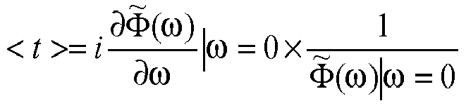
Quelle que soit la géométrie envisagée, il est possible de s'affranchir de la dépendance par rapport à la durée de vie τ, en effectuant une 4ème mesure avec un 4ème couple de positions (position de la source, position du détecteur) différent de chacun des 3 précédents. Pour de couple supplémentaire de positions (source, détecteur), on procède à l'établissement d'une TPSF ou d'un histogramme comme expliqué ci-dessus. On obtient alors l'équation d'une 4ème surface.Whatever the proposed geometry, it can be free of the dependence on the lifetime τ, by performing a measurement with a 4 th 4 th torque positions (source position, detector position) different from each of the 3 previous ones. For additional couple of positions (source, detector), one proceeds to the establishment of a TPSF or a histogram as explained above. One then obtains the equation of a 4th surface.
Comme indiqué ci-dessus dans chacun des cas traités on obtient en fait un calcul du temps moyen à partir de chaque signal de fluorescence.As indicated above in each of the treated cases, a calculation of the mean time from each fluorescence signal is actually obtained.
Il est décrit dans le document
Parmi les 4 mesures effectuées pour les 4 couples de positions, on pourra sélectionner celle qui correspond à un temps moyen mesuré minimal. L'équation de la surface qui correspond à cette mesure minimale sera soustraite de chacune des 3 autres équations.Among the 4 measurements made for the 4 pairs of positions, we can select the one that corresponds to a minimum measured average time. The surface equation corresponding to this minimum measure will be subtracted from each of the other 3 equations.
On obtiendra alors 3 nouvelles équations de 3 nouvelles surfaces, qui peuvent ne pas être des ellipsoïdes, mais à l'intersection desquelles sera localisé le fluorophore, ou bien le fluorophore sera localisé dans un volume qui contient cette intersection.We will then obtain 3 new equations of 3 new surfaces, which may not be ellipsoids, but at the intersection of which the fluorophore will be located, or the fluorophore will be located in a volume containing this intersection.
Quelle que soit la géométrie envisagée, le calcul de l'intersection de 3 ellipsoïdes, ou 3 surfaces, définis, ou définies, dans l'espace par 3 équations différentes est effectué à l'aide d'un traitement numérique mis en oeuvre par un calculateur, par exemple les moyens 24 des
Après avoir trouvé une solution avec une première précision, on peut effectuer de nouveau le calcul pour trouver une autre solution avec une deuxième précision, différente de la première.After finding a solution with a first precision, we can perform the calculation again to find another solution with a second precision, different from the first.
Chaque surface peut elle-même être définie avec une certaine précision. Ceci définit non plus une surface au sens strict, mais un volume qui s'appuie sur ladite surface. Dans le cas d'un ellipsoïde, il peut s'agir d'une couronne ellipsoïdale. Ce volume est délimité par deux surfaces, sensiblement parallèles à la surface définie strictement par l'équation correspondante et proches de celle-ci la proximité étant définie par la précision associée à la surface, qui devra être de préférence inférieure à 25%, et encore de préférence inférieure à ± 10% .Autrement dit, on cherche alors non pas l'intersection de 3 surfaces, mais de 3 volumes. Il en résulte non pas un point unique, mais l'identification d'un volume, en général suffisamment petit pour être compatible avec la localisation avec une certaine incertitude; ce volume contient l'intersection des 3 surfaces telles que définies strictement par les 3 équations initiales.Each surface can itself be defined with some precision. This no longer defines a surface in the strict sense, but a volume that leans on said surface. In the case of an ellipsoid, it may be an ellipsoidal crown. This volume is delimited by two surfaces, substantially parallel to the surface defined strictly by the corresponding equation and close to it, the proximity being defined by the precision associated with the surface, which should preferably be less than 25%, and preferably less than ± 10%. In other words, it is then not the intersection of 3 surfaces, but 3 volumes. The result is not a single point, but the identification of a volume, generally small enough to be compatible with location with some uncertainty; this volume contains the intersection of the 3 surfaces as defined strictly by the 3 initial equations.
D'une manière générale, on peut distinguer différents types d'analyse.In general, we can distinguish different types of analysis.
Il y a d'abord le cas d'une analyse invasive pour lequel source et détecteur sont placés à l'intérieur du milieu diffusant. Si la profondeur de la source et du détecteur par rapport à la frontière du milieu est suffisante, on considèrera qu'on se trouve dans les conditions d'un milieu infini (cas de la
Un premier cas d'analyse non invasive est celui pour lequel source et détecteur sont placés au contact d'une frontière du milieu diffusant (cas de la
Un deuxième cas d'analyse non invasive, est celui pour lequel source et détecteur ne sont pas en contact physique avec une frontière 21 du milieu diffusant 20, mais sont en contact optique avec le milieu. Dans ce cas, la source est par exemple un laser 8 focalisé à la surface 21 du milieu et le détecteur est un photodétecteur 4 en contact optique avec la surface du milieu (cas de la
Le premier cas non invasif peut-être combiné au second cas non invasif, la source 8 étant située à distance (comme le laser 8 de la
- la géométrie semi-infinie,
- ou la géométrie de type tranche,
- ou la géométrie de forme quelconque.
- semi-infinite geometry,
- or the slice type geometry,
- or geometry of any shape.
L'intérêt de se rapprocher de la géométrie infinie, semi-infinie ou de type tranche est de permettre d'utiliser une relation analytique reliant une grandeur mesurée (par exemple le temps moyen d'arrivée des photons) aux distances respectives source-fluorophore (ou agrégation ou accumulation locale de fluorophore) et détecteur -flurophore (ou agrégation ou accumulation locale de fluorophore). Ainsi, pour 3 acquisitions différentes, c'est-à-dire réalisée avec 3 couples différents (source - détecteur), le problème revient à déterminer les solutions satisfaisant à trois équations analytiques, ce qui peut-être entreprit rapidement à l'aide de moyens de calculs actuels. En revanche, comme décrit ci-dessous, le fait de se placer en géométrie quelconque revient à résoudre le problème de façon numérique, au détriment du temps de calcul.The interest of approaching the infinite, semi-infinite or slice-type geometry is to allow to use an analytic relation linking a measured quantity (for example the average arrival time of the photons) to the respective distances source-fluorophore ( or aggregation or local accumulation of fluorophore) and detector -flurophore (or aggregation or local accumulation of fluorophore). Thus, for 3 different acquisitions, that is to say performed with 3 different pairs (source - detector), the problem is to determine the solutions satisfying three analytical equations, which can be undertaken quickly using current calculation means. On the other hand, as described below, the fact of placing oneself in any geometry amounts to solving the problem numerically, to the detriment of the calculation time.
Dans les différents cas expliqués ci-dessus en liaison avec les
Sur ces figures, le point F désigne un fluorophore ou une agrégation de fluorophores. Mais on rappelle qu'il peut s'agir aussi d'un absorbeur (ou encore d'un fluorophore ré-émettant à la même énergie que celle d'excitation, et avec une durée τ = 0) ou d'une agrégation d'absorbeurs. Dans ce cas, le milieu 20 peut être encore un organe, la zone F identifiant une tumeur cancéreuse, visibles par le simple fait qu'elle présente un coefficient d'atténuation plus important que les tissus sains environnants.In these figures, the point F denotes a fluorophore or an aggregation of fluorophores. But it is recalled that it may also be an absorber (or a fluorophore re-emitting at the same energy as excitation, and with a duration τ = 0) or an aggregation of absorbers. In this case, the medium 20 may still be an organ, zone F identifying a cancerous tumor, visible by the simple fact that it has a greater attenuation coefficient than the surrounding healthy tissue.
Des exemples vont maintenant être décrits.Examples will now be described.
Cet exemple est un calcul en deux dimensions. Il ne concerne donc pas une mesure réelle, mais illustre la méthode dans un cas théorique, dans un plan.This example is a two-dimensional calculation. It does not concern a real measure, but illustrates the method in a theoretical case, in a plan.
Le milieu est supposé infini, à 2 dimensions, avec les propriétés optiques suivantes.The medium is assumed to be infinite, 2-dimensional, with the following optical properties.
Le coefficient de diffusion réduit est µ's = 10 cm-1 ce qui conduit à : D=1/3µ's, (cette définition de D est la plus répandue, mais il existe d'autres définitions, par exemple D=1/3(µ's+ µa), ce qui ne change rien si µa <<µ's qui définit en général le cadre de validité de l'approximation de la diffusion).The reduced scattering coefficient μ 's = 10 cm -1 which leads to: D = 1 / 3μ' s (this definition of D is the most common, but there are other definitions, for example D = 1 / 3 (μ ' s + μ a ), which does not change anything if μ a <<μ' s which generally defines the validity framework of the diffusion approximation).
Le coefficient d'absorption est µa = 0,1cm-1.The absorption coefficient is μ a = 0.1cm -1 .
On suppose en outre que les propriétés optiques sont les mêmes aux deux longueurs d'ondes, d'indice de réfraction n=1.0, ce qui donne une vitesse de propagation dans le milieu cn = 3.108/n.It is further assumed that the optical properties are the same at both wavelengths, refractive index n = 1.0, which gives a propagation speed in the medium c n = 3.10 8 / n.
Il en résulte une vitesse apparente : 
Le fluorophore choisi a un temps de vie τ=1.5 ns, ordre de grandeur classique des fluorophores que l'on utilise en imagerie moléculaire optique.The chosen fluorophore has a life time τ = 1.5 ns, a standard order of magnitude of the fluorophores that are used in optical molecular imaging.
On suppose que l'on réalise :
- une première mesure (<t>∞-τ)×ν app = 4.7000 cm, avec la source positionnée en surface du milieu en (0.0, 0.0) et un détecteur positionné en (1.0 cm,0.0). Cela signifie que le fluorophore est placé sur la demi-ellipse d'équation:

- une seconde mesure (<t>∞-τ)×ν app = 5.1000cm, avec la source positionnée en surface du milieu en (0.5 cm, 0.0) et un détecteur en (1.5 cm,0.0). Cela signifie que le fluorophore est placé sur la demi-ellipse d'équation

- a first measurement ( <t> ∞ -τ ) × ν app = 4.7000 cm, with the source positioned on the surface of the medium in (0.0, 0.0) and a detector positioned in (1.0 cm, 0.0). This means that the fluorophore is placed on the half-ellipse of equation:
- a second measurement ( <t> ∞ - τ) × ν app = 5.1000cm, with the source positioned on the surface of the medium in (0.5 cm, 0.0) and a detector in (1.5 cm, 0.0). This means that the fluorophore is placed on the equation half ellipse
La
Le montage expérimental (
La cuve 21 est remplie d'un milieu diffusant liquide 20 composé d'eau et de billes d'Acronal® (résine acrylique, BASF), ce qui conduit aux paramètres optiques suivants:
- µa = 0.01 cm-1,
- µ's = 8.7 cm-1
- μa = 0.01 cm -1 ,
- μ's = 8.7 cm -1
On considère que les propriétés optiques sont identiques à la longueur d'onde d'excitation et à celle d'émission, du fait de la proximité des longueurs d'onde d'excitation et de diffusion, suffisante pour considérer ces coefficients constants sur cette plage de longueur d'onde.It is considered that the optical properties are identical to the excitation wavelength and the emission wavelength, because of the proximity of the wavelengths of excitation and diffusion, sufficient for consider these coefficients constant over this wavelength range.
Le milieu fluorescent considéré est du Cy5 de concentration 10µMol. La durée de vie τ est de 0,96 ns, et l'indice de réfraction n0 du milieu est de 1,33.The fluorescent medium in question is Cy5 of
La
On retrouve également sur cette figure la portion des fibres 10 et 12 qui sont plongées dans le milieu examiné. L'extrémité de chaque fibre est située à 3,5 cm sous le niveau du liquide, ce qui suffit à assurer la condition de milieu infini. La puissance mesurée en sortie de fibre d'excitation 10 est de 100 µW.This figure also shows the portion of the
Sont également représentées sur cette figure les positions respectives de l'échantillon et des extrémités de fibres.Also shown in this figure are the respective positions of the sample and fiber ends.
Du point de vue de la modélisation, la source n'étant pas ponctuelle, tout se passe comme si elle devenait ponctuelle à une distance d'un libre parcours moyen de transport soit à une distance de 1/µ's (ce qui est bien le cas dans la configuration envisagée, puisque la distance entre les extrémités de fibres et l'échantillon est de 0,5 cm, tandis que 1/µ's < 0,12 cm < 0,5 cm).From the point of view of modeling, the source is not punctual, everything happens as if it became punctual at a distance of a free travel means of transport is at a distance of 1 / μ's (which is the case in the envisaged configuration, since the distance between the fiber ends and the sample is 0.5 cm, while 1 / μ's <0.12 cm <0.5 cm).
On procède à 5 mesures, avec des positions de sources et de détecteurs indiquées ci-dessous.5 measurements are made, with source and detector positions shown below.
On a sélectionné les 5 positions suivantes Si (i = 1,...5) de la source (en fait : l'extrémité de la fibre 10 ; toutes les coordonnées sont en cm):
- S1 : rs1=[0.5, 0, -3.5],
- S2 : rs2=[0, 0.25, -3.5],
- S3 : rs3= [1, 0.5, -3.5],
- S4 : rs4= [0.5, 0.5, -3.5];
- S5 : rs5= [0.5, 0.75, -3.5];
- S1: r s1 = [0.5, 0, -3.5],
- S2: r s2 = [0, 0.25, -3.5],
- S3: r s3 = [1, 0.5, -3.5],
- S4: r s4 = [0.5, 0.5, -3.5];
- S5: r s5 = [0.5, 0.75, -3.5];
Et les 5 positions suivantes Di (i = 1,...5) du détecteur (en fait : l'extrémité de la fibre 12;toutes coordonnées également en cm):
- D1: rd1=[-0.5, 0, -3.5],
- D2: rd2= [0, -0.25, -3.5],
- D3: rd3= [0, 0.5, -3.5];
- D4: rd4= [0.5, 0, -3.5] ;
- D5: rd5= [0.5, 0.25, -3.5]
- D1: r d1 = [- 0.5, 0, -3.5],
- D2: r d2 = [0, -0.25, -3.5],
- D3: r d3 = [0, 0.5, -3.5];
- D4: r d4 = [0.5, 0, -3.5];
- D5: r d5 = [0.5, 0.25, -3.5]
Pour la position Si de la source, le détecteur est en position Di.For the Si position of the source, the detector is in position Di.
La
La
Les valeurs mesurées de vapp (<t>mes1) sont les suivantes (on rappelle que <t>mes1 est le moment d'ordre 1 mesuré):
- Pour (S1, D1): 2, 2700 cm ;
- Pour (S2, D2): 2,0059 cm ;
- Pour (S3, D3): 2,7284 cm ;
- Pour (S4, D4): 2,3931 cm ;
- Pour (S5, D5): 2,5258 cm.
- For (S1, D1): 2.2700 cm;
- For (S2, D2): 2.0059 cm;
- For (S3, D3): 2.7284 cm;
- For (S4, D4): 2.3931 cm;
- For (S5, D5): 2.5258 cm.
Partant des mesures effectuées pour 3 des 5 couples de points ((S1, D1), (S3, D3) et (S4, D4)), on a calculé trois surfaces tridimensionnelles, en fait trois ellipsoïdes, conformément à l'enseignement de l'invention.From the measurements taken for 3 of the 5 pairs of points ((S1, D1), (S3, D3) and (S4, D4)), three three-dimensional surfaces, in fact three ellipsoids, were calculated in accordance with the teaching of the 'invention.
L'intersection de ces trois surfaces a également été calculée.The intersection of these three surfaces has also been calculated.
Les 3 surfaces ont été élaborées en considérant un maillage :
- En x : de 50 points entre x = -0,5 cm et x=2 cm;
- En y : de 30 points entre y = -0,5 cm et y=1 cm;
- En z : de 50 points entre z = -6 cm et z=-3,5 cm.
- In x: 50 points between x = -0.5 cm and x = 2 cm;
- In
y : 30 points between y = -0.5 cm and y = 1 cm; - In z: 50 points between z = -6 cm and z = -3.5 cm.
Le fluorophore a été localisé en position (x1,y1,z1) suivante :
- -0,041<x1<0,062;
- 0,12<y1<0,17
- -0,91<z1<-3,81.
- -0.041 <x 1 <0.062;
- 0.12 <y 1 <0.17
- -0.91 <z 1 <-3.81.
On rappelle que la position réelle est (0,0, -4). Les
Le temps nécessaire pour ces calculs, pour le maillage choisi (avec le maillage retenu) avec un logiciel « Matlab », sur processeur Intel Core2, à 2.13GHz, avec 1Go de RAM est inférieur à 3 secondes:
- durée du calcul des distances di pour les trois couples (Si, Di) sélectionnés: 2,6 s
- durée du calcul des équations des 3 ellipsoïdes (ξ1, ξ2, et ξ3): 0,12 s
- durée du calcul de la détermination de l'intersection : 0,04 s.
- duration of the calculation of the distances di for the three couples (Si, Di) selected: 2.6 s
- calculation time of the equations of the 3 ellipsoids (ξ1, ξ2, and ξ3): 0.12 s
- calculation duration of the intersection determination: 0.04 s.
La durée totale de calcul avec un matériel informatique standard est tout à fait compatible avec une mesure sur ou dans un organe du corps humain, par exemple lors d'une intervention chirurgicale ou dans une unité d'analyse.The total computation time with standard computer hardware is quite compatible with a measurement on or in an organ of the human body, for example during a surgical procedure or in a unit of analysis.
Le calcul a ensuite été refait, en prenant en compte l'ensemble des 5 mesures : on a donc calculé l'intersection des 5 surfaces.The calculation was then redone, taking into account all the 5 measurements: we thus calculated the intersection of the 5 surfaces.
Le fluorophore a alors été localisé en position (x2,y2,z2) = (0,06; 0,12; 3,91). Cette nouvelle position est assez proche de la précédente : la localisation effectuée avec seulement trois surfaces est donc suffisante.The fluorophore was then located in position (x 2 , y 2 , z 2 ) = (0.06, 0.12, 3.91). This new position is quite close to the previous one: the location made with only three surfaces is therefore sufficient.
Cet exemple est en trois dimensions, et en milieu semi-infini.This example is in three dimensions, and in semi-infinite medium.
On considère 3 couples de positions de la source et du détecteur (rs, rd).We consider 3 pairs of positions of the source and detector (r s , r d ).
Par exemple, on a les 3 positions suivantes de la source (toutes les coordonnées sont en cm): rs1=[0.0, 0, 0], rs2= [0.5, 0, 0], rs3= [0.75, -1, 0];For example, we have the following 3 positions of the source (all coordinates are in cm): r s1 = [0.0, 0, 0], r s2 = [0.5, 0, 0], r s3 = [0.75, - 1, 0];
Et les 3 positions suivantes du détecteur (toutes coordonnées également en cm):
- rd1=[1.0, 0, 0], rd2= [1.5, 0, 0], rd3= [0.75, 0, 5, 0]
- r d1 = [1.0, 0, 0], r d2 = [1.5, 0, 0], r d3 = [0.75, 0, 5, 0]
Ces 3 couples sont représentés en
Les propriétés optiques sont les mêmes que dans l'exemple précédent.The optical properties are the same as in the previous example.
On suppose que l'on réalise :
- une première mesure (<t>∞-τ)×ν app = 4.6000 cm, pour le couple de positions (rs1, rd1),
- une deuxième mesure (<t>∞-τ)×ν app = 5.6000 cm, pour le couple de positions (rs2, rd2),
- une troisième mesure (<t>∞-τ)×ν app = 4.6000 cm, pour le couple de positions (rs3, rd3).
- a first measurement ( <t> ∞ -τ ) × ν app = 4.6000 cm, for the pair of positions (r s1 , r d1 ),
- a second measurement (<t> ∞ - τ) × ν app = 5.6000 cm, for the pair of positions (r s2 , r d2 ),
- a third measurement ( <t> ∞ -τ ) × ν app = 4.6000 cm, for the pair of positions (r s3 , r d3 ).
Alors la position du fluorophore appartient à l'intersection des ellipsoïdes, qui ont pour équations suivantes: ![]()
![]()
![]()
![]()
![]()
![]()
Sur chacune des
La zone d'intersection de ces 3 ellipsoïdes est identifiée par la zone I en
Les figures ont été élaborées en considérant un maillage :
- En x : de 101 points entre x = -2 et x=3;
- En y : de 101 points entre x = -2 et x=2;
- En z : de 101 points entre x = -3 et x=0;
- In x: of 101 points between x = -2 and x = 3;
- In y: of 101 points between x = -2 and x = 2;
- In z: 101 points between x = -3 and x = 0;
La solution de la
Il est possible d'imposer une précision plus importante. Ainsi, en
- En
figure 6B : solution à 2% près, - En
figure 6C : solution à 1,4% près.
- In
Figure 6B : 2% solution, - In
Figure 6C : solution to 1.4%.
On voit que l'accroissement de précision apporte peu d'information supplémentaire pour une localisation approchée du fluorophore.It can be seen that the increase in precision provides little additional information for an approximate location of the fluorophore.
Il est intéressant d'évaluer le temps nécessaire pour ces calculs, avec un logiciel « Matlab », sur processeur Intel Core2, à 2.13GHz, avec 1Go de RAM:
- pour le calcul des moments pour les 3 couples source-détecteur en chaque point du maillage : 5.6835 s,
- pour le calcul des équations des 3 ellipsoïdes (ξ1, ξ2, et ξ3): 2.086609 s,
- pour le calcul de la détermination de l'intersection : 2.253164 s.
- for the calculation of the moments for the 3 source-detector pairs at each point of the mesh: 5.6835 s,
- for the calculation of the equations of the 3 ellipsoids (ξ1, ξ2, and ξ3): 2.086609 s,
- for the calculation of the determination of the intersection: 2.253164 s.
Il en résulte une durée totale d'environ 10 s pour le maillage choisi.This results in a total duration of about 10 s for the chosen mesh.
Ce résultat illustre bien le caractère « temps réel » ou rapide du procédé.This result is a good illustration of the "real time" or fast nature of the process.
Dans le cadre d'une application chirurgicale, un praticien peut réaliser une analyse selon l'invention alors même qu'il est en présence d'un patient. Une durée de 10 s, ou même une durée légèrement supérieure, est tout à fait compatible avec le maintien d'un patient sur une table d'opération ou dans une salle d'analyse.In the context of a surgical application, a practitioner may perform an analysis according to the invention even though it is in the presence of a patient. A duration of 10 seconds, or even a slightly longer duration, is entirely compatible with keeping a patient on an operating table or in an analysis room.
La détermination de la position du fluorophore dépend de son temps de vie. Pour s'en affranchir, on peut considérer des mesures différentielles, comme expliqué dans la demande de brevet
Par exemple :
- Avec les configurations de sources-détecteurs ci-dessus, en milieu semi-infini, on a les ellipsoïdes suivants :


- With the above detector-source configurations, in a semi-infinite environment, we have the following ellipsoids:
Le 3ème correspond à une mesure dont le trajet optique est le plus court des trois. C'est cette mesure qui, comme expliqué dans la demande
Si l'on considère les quantités ![]()
et ![]()
on obtient des relations indépendantes du temps de vie.If we consider the quantities ![]()
and ![]()
we obtain relations independent of the life time.
Ces quantités ne définissent plus des ellipsoïdes mais des surfaces plus complexes.These quantities no longer define ellipsoids but more complex surfaces.
Les
En 3D, une troisième surface est nécessaire pour identifier une localisation possible du fluorophore.In 3D, a third surface is needed to identify a possible location of the fluorophore.
On considère donc un ensemble, non pas de 3 mesures, mais de 4 mesures.So we consider a set, not of 3 measures, but of 4 measures.
Par exemple, on a les 4 positions suivantes de la source (toutes les coordonnées sont en cm): rs1=[0.0, 0, 0], rs2= [0.5, 0, 0], rs3= [0.75, -1, 0]; rs4= [-0.75 ; -1.5 ; 0];For example, we have the following 4 positions of the source (all coordinates are in cm): r s1 = [0.0, 0, 0], r s2 = [0.5, 0, 0], r s3 = [0.75, - 1, 0]; r s4 = [-0.75; -1.5; 0];
Et les 4 positions suivantes du détecteur (toutes coordonnées également en cm):
- rd1=[1.0, 0, 0], rd2= [1.5, 0, 0], rd3= [0.75, 0,5, 0] ; rd4= [0.75, 1, 0].
- r d1 = [1.0, 0, 0], r d2 = [1.5, 0, 0], r d3 = [0.75, 0.5, 0]; r d4 = [0.75, 1, 0].
On obtient donc, outre les 3 surfaces ξ1, ξ2, ξ3 déjà définies, une surface ξ4 (qui définit elle aussi un ellipsoïde) : ![]()
![]()
Cette surface ξ4 va elle aussi être normalisée. On effectue donc la différence ξ4-ξ3 qui définit elle-même une surface dont l'intersection avec les surfaces ξ1-ξ3 et ξ2-ξ3 va permettre de localiser le fluorophore.This surface ξ 4 will also be normalized. We thus make the difference ξ 4 -ξ 3 which defines itself a surface whose intersection with the surfaces ξ 1 -ξ 3 and ξ 2 -ξ 3 will allow to locate the fluorophore.
La
La zone d'intersection des 3 surfaces, et donc la zone de localisation du fluorophore est identifiée par la zone P sur cette
Cet exemple est en trois dimensions, et en géométrie de type « slab ».This example is in three dimensions, and in "slab" type geometry.
La tranche considérée est d'épaisseur L = 1, 5 cm.The slice in question is of thickness L = 1.5 cm.
On considère 3 couples de positions de la source et du détecteur (rs, rd).We consider 3 pairs of positions of the source and detector (r s , r d ).
Par exemple, on a les 3 positions suivantes de la source (toutes les coordonnées sont en cm): rs1=[0.0, 0, 0], rs2= [0.5, 0, 0], rs3= [0.75, -1, 0];For example, we have the following 3 positions of the source (all coordinates are in cm): r s1 = [0.0, 0, 0], r s2 = [0.5, 0, 0], r s3 = [0.75, - 1, 0];
Et les 3 positions suivantes du détecteur (toutes coordonnées également en cm):
- rd1=[1.0, 0, 0], rd2= [1.5, 0, 0], rd3= [0.75, 0, 5, 0]
- r d1 = [1.0, 0, 0], r d2 = [1.5, 0, 0], r d3 = [0.75, 0, 5, 0]
Comme pour les exemples précédents, on obtient la définition de trois ellipsoïdes, pour les trois valeurs suivantes de vapp (<t>mes) : 1,84 ; 1,93 ; 1,81.As for the previous examples, we obtain the definition of three ellipsoids, for the following three values of v app (<t> mes ): 1.84; 1.93; 1.81.
Sur chacun des
Sur ces figures, la tranche constituant le milieu est délimitée par les deux plans parallèles: Z = 0 et Z = - 1,5 cm.In these figures, the slice constituting the medium is delimited by the two parallel planes: Z = 0 and Z = -1.5 cm.
La zone d'intersection de ces 3 ellipsoïdes est identifiée par la zone I en
De manière générale, un exemple de procédé selon l'invention peut être mis en oeuvre selon le schéma représenté en
Les étapes de cet exemple, et d'ailleurs de toute autre mise en oeuvre d'un procédé selon l'invention, peuvent être précédées d'une étape - non représentée - d'injection dans le milieu étudié d'au moins un fluorophore ou absorbeur destiné à venir se fixer sur une zone d'intérêt. En fait lorsqu'on injecte un fluorophore, on en injecte souvent plusieurs. On peut d'ailleurs assimiler une zone fluorescente à une agglomération de fluorophores. Il n'y a généralement pas qu'une seule molécule fluorescente, mais une concentration locale de molécules fluorescentes. De la même façon, lorsqu'on travaille en absorption, il n'y a pas qu'une seule molécule absorbante, mais une concentration de molécules absorbantes. Cette concentration peut être considérée comme ponctuelle si la distance la séparant du détecteur est suffisamment grande devant ses dimensions. Typiquement, une concentration de rayon r est considérée comme ponctuelle, à une distance d'observation d donnée, si d > 10 r. Certains absorbeurs peuvent déjà être dans le milieu, par exemple lorsqu'il s'agit d'une zone présentant une absorption différente de son environnement.The steps of this example, and moreover of any other implementation of a method according to the invention, may be preceded by a step - not shown - of injection into the medium studied of at least one fluorophore or absorber intended to be fixed on an area of interest. In fact, when a fluorophore is injected, many are often injected. We can also assimilate a fluorescent zone to an agglomeration of fluorophores. There is usually not just one fluorescent molecule, but one local concentration of fluorescent molecules. In the same way, when working in absorption, there is not only one absorbing molecule, but a concentration of absorbing molecules. This concentration can be considered as point if the distance separating it from the detector is sufficiently large in front of its dimensions. Typically, a concentration of radius r is considered as point, at a given observation distance d, if d> 10 r. Some absorbers may already be in the medium, for example when it is a zone with a different absorption of its environment.
On positionne ensuite les moyens d'émission de rayonnement et de détection par rapport au milieu. L'une des configurations déjà décrites peut être sélectionnée. En particulier on peut réaliser un examen invasif u non invasif.The radiation emission and detection means are then positioned relative to the medium. One of the configurations already described can be selected. In particular, a non-invasive invasive examination can be performed.
Au cours d'une première étape S1 de ce procédé, les données, ou paramètres, d'entrée sont fournis: il s'agit des propriétés optiques du milieu diffusant, aux deux longueurs d'onde de d'excitation et d'émission (dans certains cas, à ces deux longueurs d'onde, les propriétés optiques sont identiques), la géométrie du milieu, les positions des sources et du détecteur (au sens déjà expliqué ci-dessus), et le choix du maillage pour le calcul des surfaces. Au cours d'une deuxième étape (S2), les fichiers de mesures (TPSF) pour chaque couple source-détecteur sont lus. Un prétraitement des données peut être réalisé.During a first step S1 of this method, input data or parameters are provided: these are the optical properties of the scattering medium, at the two wavelengths of excitation and emission ( in some cases, at these two wavelengths, the optical properties are identical), the geometry of the medium, the positions of the sources and the detector (in the sense already explained above), and the choice of the mesh for the calculation of the surfaces. During a second step (S2), the measurement files (TPSF) for each source-detector pair are read. Preprocessing of the data can be done.
A partir des données introduites lors de la première étape, une expression analytique de chaque surface va pouvoir être déterminée ou calculée pour chaque point du maillage (étape S3).From the data introduced during the first step, an analytic expression of each surface will be able to be determined or calculated for each point of the mesh (step S3).
Les données issues de l'étape S2 vont permettre un calcul des temps moyens <ti> pour chacune des mesures effectuées (étape S4).The data from step S2 will allow a calculation of mean times <t i > for each of the measurements made (step S4).
Les étapes S1 et S3 d'une part, S2 et S34 d'autre part, sont représentées en
A partir des données de calcul des étapes S3 et S4, on recherche les points du maillage tels que ξi = <ti>, pour tout i, à X% près (étape S5), ce qui signifie |ξi- <ti> | ≤ X/100. L'utilisateur peut lui- même fixer la précision X souhaitée.From the calculation data of steps S3 and S4, the points of the mesh are searched such that ξ i = <t i >, for all i, to within X% (step S5), which means | ξ i - <t i > | ≤ X / 100. The user can himself set the desired X precision.
Les résultats (l'intersection des surfaces entre elle, et éventuellement chacune des surfaces individuellement) peuvent ensuite être visualisés (étape S6).The results (the intersection of the surfaces between it, and possibly each of the surfaces individually) can then be viewed (step S6).
Au besoin, les calculs peuvent être réitérés en fixant une valeur de X supérieure (auquel cas on réduit la précision) ou inférieure (auquel cas on accroît la précision) à la valeur précédente (étape S7).If necessary, the calculations can be reiterated by setting a value of X higher (in which case the precision is reduced) or lower (in which case the precision is increased) to the previous value (step S7).
Claims (15)
- Method of localising at least one fluorophore (22) or at least one absorber in a scattering medium (20), by means of a device comprising a pulse radiation source (8, 10) suited to emitting an excitation radiation of this fluorophore or this molecule and detection means (4, 12) suited to measuring a fluorescence signal emitted by this fluorophore (22) or an emission signal emitted by this absorber, said device allowing a time resolved detection of these signals, the method being characterized in that it comprises:a) for at least 3 different pairs of positions of the radiation source and detection means, at least one excitation by a radiation coming from the radiation source (8), and at least one detection by the means (4) of detecting the fluorescence signal emitted by this fluorophore after this excitation, or of the emission signal emitted by this absorber,b) for each of these pairs, the identification of a surface on which the fluorophore or the absorber is situated, or of a volume comprising this surface and in which the fluorophore or the absorber is situated, this identification comprising the calculation of a moment of order n≥1 of said fluorescence signal or of said emission signal or of a frequency function of said fluorescence signal or of said emission signal,c) an estimation of the localisation of the fluorophore or the absorber in its scattering medium, by calculation of the intersection of the three surfaces, and possibly of a volume around this intersection.
- Method according to claim 1, wherein the diffusing medium, surrounding the fluorophore or the absorber is of infinite type or semi-infinite type or forms a slab, limited by two parallel surfaces, or is of any shape, its exterior surface being discretised into a series of planes.
- Method according to any of claims 1 or 2, wherein the scattering medium is of infinite type, the surfaces then having the shape of ellipsoids.
- Method according to any of claims 1 to 3, step b) comprising, for each position pair, a calculation of a normalised time moment, of a time function of the fluorescence signal or of the emission signal by the absorber, or of a normalised moment of a frequency function, deduced from said time function of the fluorescence signal or the emission signal by the absorber.
- Method according to claim 4, the frequency function being deduced from said time function by Fourier transform or by Laplace transform or by Mellin transform.
- Method according to any of claims 1 to 5, wherein an excitation is carried out by the radiation source (8), and a detection by the detection means (4) for 4 different pairs of positions of the radiation source and detection means.
- Method according to claim 6, wherein, for the localisation of at least one fluorophore:- among the four pairs of points are selected the pair of points, known as fourth pair of points, for which the average arrival time of the photons, from the time of emission by the emitter to the time of reception by the receiver, is the shortest, and, for this pair of points, the equation of a surface on which the fluorophore is situated is calculated,- and, for each of the three other pairs of points, a first equation of a first surface on which the fluorophore is situated is calculated, and a difference is taken between this equation and that associated with the fourth pair, to obtain a second equation of a second surface independent of the lifetime of the fluorophore
- Method according to any of claims 1 to 6, wherein, for the localisation of at least one fluorophore (22), step b) comprises, for each position pair, a calculation of an equation of each surface, independent of the lifetime of the fluorophore.
- Method according to claim 8, said equation independent of τ resulting from the difference between the average time measured or calculated for each position pair and the average time measured or calculated for a fourth position pair.
- Method according to claim 9, the fourth position pair being a pair for which the fluorescence signal has a measured average time or a calculated average time less than that of the 3 position pairs.
- Method according to any of claims 1 to 10, the radiation source being the end of an optic fibre (10) which sends light into the medium and/or and the detection means being the end of an optic fibre (12), which samples a part of the emission light.
- Device for the localisation of at least one fluorophore or at least one absorber in a scattering medium, comprising:- a pulse radiation source (8, 10) suited to emitting an excitation radiation,- detection means (4, 12) suited to measuring a fluorescence signal emitted by this fluorophore (22) or an emission signal emitted by this absorber,- the device allowing a time resolved detection of these signals,this device being characterized in that it comprises:calculation means for:a) for each pair of points among at least 3 different pairs of positions of the radiation source and detection means, carrying out a calculation or determining, comprising the calculation of a moment of order n > 1 of said fluorescence signal or said emission signal, after an excitation carried out by a radiation coming from the radiation source (8), and a detection by the means (4) of detecting signals emitted by the fluorophore or the absorber after this excitation, of a surface on which the fluorophore or the absorber is situated, or a volume comprising this surface and in which the fluorophore or the absorber is situated,b) and for estimating the localisation of the fluorophore or the absorber in its surrounding medium, by calculation of the intersection of the three surfaces or of a volume around this intersection.
- Device according to claim 12, the calculation means making it possible to calculate, for each position pair, a normalised time moment of a time function, or a normalised moment of a frequency function, deduced from said emission time function.
- Device according to claim 12 or 13, said detection means comprising TCSPC type means or camera type means.
- Device according to one of claims 12 to 14, further comprising means of visual or graphic representation of the localisation of the fluorophore or the absorbent molecule.
Applications Claiming Priority (1)
| Application Number | Priority Date | Filing Date | Title |
|---|---|---|---|
| FR0857699A FR2938181B1 (en) | 2008-11-13 | 2008-11-13 | METHOD AND DEVICE FOR LOCATING FLUOROPHORES OR ABSORBERS IN A SURROUNDING ENVIRONMENT |
Publications (2)
| Publication Number | Publication Date |
|---|---|
| EP2186469A1 EP2186469A1 (en) | 2010-05-19 |
| EP2186469B1 true EP2186469B1 (en) | 2015-04-29 |
Family
ID=40723193
Family Applications (1)
| Application Number | Title | Priority Date | Filing Date |
|---|---|---|---|
| EP20090175560 Active EP2186469B1 (en) | 2008-11-13 | 2009-11-10 | Method and device for the localisation of fluorophores or absorbers in surrounding medium |
Country Status (3)
| Country | Link |
|---|---|
| US (1) | US8263947B2 (en) |
| EP (1) | EP2186469B1 (en) |
| FR (1) | FR2938181B1 (en) |
Families Citing this family (16)
| Publication number | Priority date | Publication date | Assignee | Title |
|---|---|---|---|---|
| FR2984503B1 (en) * | 2011-12-16 | 2014-01-17 | Commissariat Energie Atomique | METHOD FOR RECONSTRUCTING OPTICAL PROPERTIES OF A DIFFUSING MEDIUM USING A COMBINATION OF A PLURALITY OF MELLIN-LAPLACE TRANSFORMS OF A SIZE INCLUDING A TIME DISTRIBUTION OF A RECEIVED SIGNAL, AND ASSOCIATED RECONSTRUCTION SYSTEM |
| FR3032527B1 (en) | 2015-02-06 | 2020-03-13 | Commissariat A L'energie Atomique Et Aux Energies Alternatives | DEVICE FOR MEASURING AN OPTICAL SIGNAL BACKPACKED BY A SAMPLE |
| US9730649B1 (en) | 2016-09-13 | 2017-08-15 | Open Water Internet Inc. | Optical imaging of diffuse medium |
| US10778911B2 (en) | 2018-03-31 | 2020-09-15 | Open Water Internet Inc. | Optical transformation device for imaging |
| US10778912B2 (en) | 2018-03-31 | 2020-09-15 | Open Water Internet Inc. | System and device for optical transformation |
| US10506181B2 (en) | 2018-03-31 | 2019-12-10 | Open Water Internet Inc. | Device for optical imaging |
| US10966612B2 (en) | 2018-06-14 | 2021-04-06 | Open Water Internet Inc. | Expanding beam optical element |
| US10962929B2 (en) | 2018-09-14 | 2021-03-30 | Open Water Internet Inc. | Interference optics for optical imaging device |
| US10874370B2 (en) | 2019-01-28 | 2020-12-29 | Open Water Internet Inc. | Pulse measurement in optical imaging |
| US10955406B2 (en) | 2019-02-05 | 2021-03-23 | Open Water Internet Inc. | Diffuse optical imaging with multiple beams |
| US11320370B2 (en) | 2019-06-26 | 2022-05-03 | Open Water Internet Inc. | Apparatus for directing optical and acoustic signals |
| US11581696B2 (en) | 2019-08-14 | 2023-02-14 | Open Water Internet Inc. | Multi-channel laser |
| US11622686B2 (en) | 2019-11-22 | 2023-04-11 | Open Water Internet, Inc. | Optical imaging with unshifted reference beam |
| US11819318B2 (en) | 2020-04-27 | 2023-11-21 | Open Water Internet Inc. | Optical imaging from light coherence |
| US11559208B2 (en) | 2020-05-19 | 2023-01-24 | Open Water Internet Inc. | Imaging with scattering layer |
| US11259706B2 (en) | 2020-05-19 | 2022-03-01 | Open Water Internet Inc. | Dual wavelength imaging and out of sample optical imaging |
Family Cites Families (4)
| Publication number | Priority date | Publication date | Assignee | Title |
|---|---|---|---|---|
| US5353799A (en) * | 1991-01-22 | 1994-10-11 | Non Invasive Technology, Inc. | Examination of subjects using photon migration with high directionality techniques |
| US6058324A (en) * | 1993-06-17 | 2000-05-02 | Non-Invasive Technology, Inc. | Examination and imaging of biological tissue |
| CA2581592C (en) | 2004-09-24 | 2014-04-15 | New Art Advanced Research Technologies Inc. | Method for fluorescence tomographic imaging |
| FR2904691B1 (en) | 2006-08-02 | 2009-03-06 | Commissariat Energie Atomique | METHOD AND DEVICE FOR 3D RECONSTRUCTION OF THE DISTRIBUTION OF FLUORESCENT ELEMENTS |
-
2008
- 2008-11-13 FR FR0857699A patent/FR2938181B1/en not_active Expired - Fee Related
-
2009
- 2009-11-10 EP EP20090175560 patent/EP2186469B1/en active Active
- 2009-11-11 US US12/616,502 patent/US8263947B2/en active Active
Also Published As
| Publication number | Publication date |
|---|---|
| US20100155622A1 (en) | 2010-06-24 |
| EP2186469A1 (en) | 2010-05-19 |
| FR2938181B1 (en) | 2012-03-09 |
| US8263947B2 (en) | 2012-09-11 |
| FR2938181A1 (en) | 2010-05-14 |
Similar Documents
| Publication | Publication Date | Title |
|---|---|---|
| EP2186469B1 (en) | Method and device for the localisation of fluorophores or absorbers in surrounding medium | |
| EP2605002B1 (en) | Method for reconstructing the optical properties of a scattering medium using a combination of a plurality of Mellin-Laplace transforms of a magnitude comprising a time distribution of a received signal, and associated reconstruction system | |
| EP2182343B1 (en) | Method and device for measuring the optical characteristics of an object | |
| EP2606817B1 (en) | System for reconstructing optical properties of a scattering medium, including a source of pulsed radiation and at least two detectors of two different types, and associated reconstruction method | |
| EP1884765B1 (en) | Method and device for the 3D reconstruction of the distribution of fluorescent elements | |
| EP2465416B1 (en) | Method for locating an optical marker in a diffusing medium | |
| EP3295153B1 (en) | Method of correcting a fluorescence image | |
| EP2302362B1 (en) | Device and method for spatial reconstruction of a fluorescence cartography | |
| CN101612034B (en) | Time-resolved measurement system and method for reconstructing optical parameters of turbid media | |
| US20090164130A1 (en) | Fluorescence-lifetime-based tomography | |
| Gavgiotaki et al. | Third Harmonic Generation microscopy distinguishes malignant cell grade in human breast tissue biopsies | |
| JP2009538418A (en) | Photoacoustic imaging method | |
| EP2033030A2 (en) | Optical fluorescence tomography calibration | |
| Sinha et al. | Comparison of time-and angular-domain scatter rejection in mesoscopic optical projection tomography: a simulation study | |
| Boutet et al. | Bimodal ultrasound and fluorescence approach for prostate cancer diagnosis | |
| JP5183406B2 (en) | Biological information processing apparatus and biological information processing method | |
| EP1994505B1 (en) | Method of reconstructing an optical tomography image by fluorescence of an object having any outline | |
| Qu et al. | Excitation-and-collection geometry insensitive fluorescence imaging of tissue-simulating turbid media | |
| EP2991544B1 (en) | Method and device for locating at least one target in an electromagnetically absorbent environment | |
| EP3054284B1 (en) | Method for correcting a raman signal backscattered by a sample, and associated device | |
| EP4023147B1 (en) | Method for analysing a sample by resolute measurement over time of the intensity of backscattered photons | |
| EP2605000B1 (en) | System and method for reconstruction of the optical properties of a medium with calculation of a corrected signal depending on a first model function for a reference medium and a second distribution within the medium to be characterised | |
| Lu et al. | Parallelized Monte Carlo photon transport simulations for arbitrary multi-angle wide-field illumination in optoacoustic imaging | |
| EP2405800A1 (en) | Fluorescence image processing by non-negative matrix factorisation | |
| Hervé et al. | Localization of fluorescence marked prostate tumor with time-resolved diffuse optical tomography |
Legal Events
| Date | Code | Title | Description |
|---|---|---|---|
| PUAI | Public reference made under article 153(3) epc to a published international application that has entered the european phase |
Free format text: ORIGINAL CODE: 0009012 |
|
| AK | Designated contracting states |
Kind code of ref document: A1 Designated state(s): AT BE BG CH CY CZ DE DK EE ES FI FR GB GR HR HU IE IS IT LI LT LU LV MC MK MT NL NO PL PT RO SE SI SK SM TR |
|
| AX | Request for extension of the european patent |
Extension state: AL BA RS |
|
| 17P | Request for examination filed |
Effective date: 20101116 |
|
| GRAJ | Information related to disapproval of communication of intention to grant by the applicant or resumption of examination proceedings by the epo deleted |
Free format text: ORIGINAL CODE: EPIDOSDIGR1 |
|
| GRAP | Despatch of communication of intention to grant a patent |
Free format text: ORIGINAL CODE: EPIDOSNIGR1 |
|
| GRAP | Despatch of communication of intention to grant a patent |
Free format text: ORIGINAL CODE: EPIDOSNIGR1 |
|
| INTG | Intention to grant announced |
Effective date: 20141126 |
|
| RIN1 | Information on inventor provided before grant (corrected) |
Inventor name: DINTEN, JEAN-MARC Inventor name: DA SILVA, ANABELA Inventor name: RIZO, PHILIPPE |
|
| GRAS | Grant fee paid |
Free format text: ORIGINAL CODE: EPIDOSNIGR3 |
|
| GRAA | (expected) grant |
Free format text: ORIGINAL CODE: 0009210 |
|
| AK | Designated contracting states |
Kind code of ref document: B1 Designated state(s): AT BE BG CH CY CZ DE DK EE ES FI FR GB GR HR HU IE IS IT LI LT LU LV MC MK MT NL NO PL PT RO SE SI SK SM TR |
|
| REG | Reference to a national code |
Ref country code: GB Ref legal event code: FG4D Free format text: NOT ENGLISH |
|
| REG | Reference to a national code |
Ref country code: CH Ref legal event code: EP |
|
| REG | Reference to a national code |
Ref country code: AT Ref legal event code: REF Ref document number: 723982 Country of ref document: AT Kind code of ref document: T Effective date: 20150515 |
|
| REG | Reference to a national code |
Ref country code: IE Ref legal event code: FG4D Free format text: LANGUAGE OF EP DOCUMENT: FRENCH |
|
| REG | Reference to a national code |
Ref country code: DE Ref legal event code: R096 Ref document number: 602009030930 Country of ref document: DE Effective date: 20150603 |
|
| REG | Reference to a national code |
Ref country code: NL Ref legal event code: VDEP Effective date: 20150429 |
|
| REG | Reference to a national code |
Ref country code: AT Ref legal event code: MK05 Ref document number: 723982 Country of ref document: AT Kind code of ref document: T Effective date: 20150429 |
|
| REG | Reference to a national code |
Ref country code: LT Ref legal event code: MG4D |
|
| PG25 | Lapsed in a contracting state [announced via postgrant information from national office to epo] |
Ref country code: NL Free format text: LAPSE BECAUSE OF FAILURE TO SUBMIT A TRANSLATION OF THE DESCRIPTION OR TO PAY THE FEE WITHIN THE PRESCRIBED TIME-LIMIT Effective date: 20150429 |
|
| PG25 | Lapsed in a contracting state [announced via postgrant information from national office to epo] |
Ref country code: ES Free format text: LAPSE BECAUSE OF FAILURE TO SUBMIT A TRANSLATION OF THE DESCRIPTION OR TO PAY THE FEE WITHIN THE PRESCRIBED TIME-LIMIT Effective date: 20150429 Ref country code: LT Free format text: LAPSE BECAUSE OF FAILURE TO SUBMIT A TRANSLATION OF THE DESCRIPTION OR TO PAY THE FEE WITHIN THE PRESCRIBED TIME-LIMIT Effective date: 20150429 Ref country code: PT Free format text: LAPSE BECAUSE OF FAILURE TO SUBMIT A TRANSLATION OF THE DESCRIPTION OR TO PAY THE FEE WITHIN THE PRESCRIBED TIME-LIMIT Effective date: 20150831 Ref country code: NO Free format text: LAPSE BECAUSE OF FAILURE TO SUBMIT A TRANSLATION OF THE DESCRIPTION OR TO PAY THE FEE WITHIN THE PRESCRIBED TIME-LIMIT Effective date: 20150729 Ref country code: HR Free format text: LAPSE BECAUSE OF FAILURE TO SUBMIT A TRANSLATION OF THE DESCRIPTION OR TO PAY THE FEE WITHIN THE PRESCRIBED TIME-LIMIT Effective date: 20150429 Ref country code: FI Free format text: LAPSE BECAUSE OF FAILURE TO SUBMIT A TRANSLATION OF THE DESCRIPTION OR TO PAY THE FEE WITHIN THE PRESCRIBED TIME-LIMIT Effective date: 20150429 |
|
| PG25 | Lapsed in a contracting state [announced via postgrant information from national office to epo] |
Ref country code: GR Free format text: LAPSE BECAUSE OF FAILURE TO SUBMIT A TRANSLATION OF THE DESCRIPTION OR TO PAY THE FEE WITHIN THE PRESCRIBED TIME-LIMIT Effective date: 20150730 Ref country code: AT Free format text: LAPSE BECAUSE OF FAILURE TO SUBMIT A TRANSLATION OF THE DESCRIPTION OR TO PAY THE FEE WITHIN THE PRESCRIBED TIME-LIMIT Effective date: 20150429 Ref country code: LV Free format text: LAPSE BECAUSE OF FAILURE TO SUBMIT A TRANSLATION OF THE DESCRIPTION OR TO PAY THE FEE WITHIN THE PRESCRIBED TIME-LIMIT Effective date: 20150429 Ref country code: IS Free format text: LAPSE BECAUSE OF FAILURE TO SUBMIT A TRANSLATION OF THE DESCRIPTION OR TO PAY THE FEE WITHIN THE PRESCRIBED TIME-LIMIT Effective date: 20150829 |
|
| REG | Reference to a national code |
Ref country code: FR Ref legal event code: PLFP Year of fee payment: 7 |
|
| PG25 | Lapsed in a contracting state [announced via postgrant information from national office to epo] |
Ref country code: DK Free format text: LAPSE BECAUSE OF FAILURE TO SUBMIT A TRANSLATION OF THE DESCRIPTION OR TO PAY THE FEE WITHIN THE PRESCRIBED TIME-LIMIT Effective date: 20150429 Ref country code: EE Free format text: LAPSE BECAUSE OF FAILURE TO SUBMIT A TRANSLATION OF THE DESCRIPTION OR TO PAY THE FEE WITHIN THE PRESCRIBED TIME-LIMIT Effective date: 20150429 |
|
| REG | Reference to a national code |
Ref country code: DE Ref legal event code: R097 Ref document number: 602009030930 Country of ref document: DE |
|
| PG25 | Lapsed in a contracting state [announced via postgrant information from national office to epo] |
Ref country code: SK Free format text: LAPSE BECAUSE OF FAILURE TO SUBMIT A TRANSLATION OF THE DESCRIPTION OR TO PAY THE FEE WITHIN THE PRESCRIBED TIME-LIMIT Effective date: 20150429 Ref country code: RO Free format text: LAPSE BECAUSE OF NON-PAYMENT OF DUE FEES Effective date: 20150429 Ref country code: CZ Free format text: LAPSE BECAUSE OF FAILURE TO SUBMIT A TRANSLATION OF THE DESCRIPTION OR TO PAY THE FEE WITHIN THE PRESCRIBED TIME-LIMIT Effective date: 20150429 Ref country code: PL Free format text: LAPSE BECAUSE OF FAILURE TO SUBMIT A TRANSLATION OF THE DESCRIPTION OR TO PAY THE FEE WITHIN THE PRESCRIBED TIME-LIMIT Effective date: 20150429 |
|
| PLBE | No opposition filed within time limit |
Free format text: ORIGINAL CODE: 0009261 |
|
| STAA | Information on the status of an ep patent application or granted ep patent |
Free format text: STATUS: NO OPPOSITION FILED WITHIN TIME LIMIT |
|
| 26N | No opposition filed |
Effective date: 20160201 |
|
| PG25 | Lapsed in a contracting state [announced via postgrant information from national office to epo] |
Ref country code: IT Free format text: LAPSE BECAUSE OF FAILURE TO SUBMIT A TRANSLATION OF THE DESCRIPTION OR TO PAY THE FEE WITHIN THE PRESCRIBED TIME-LIMIT Effective date: 20150429 |
|
| PG25 | Lapsed in a contracting state [announced via postgrant information from national office to epo] |
Ref country code: SI Free format text: LAPSE BECAUSE OF FAILURE TO SUBMIT A TRANSLATION OF THE DESCRIPTION OR TO PAY THE FEE WITHIN THE PRESCRIBED TIME-LIMIT Effective date: 20150429 |
|
| PG25 | Lapsed in a contracting state [announced via postgrant information from national office to epo] |
Ref country code: MC Free format text: LAPSE BECAUSE OF FAILURE TO SUBMIT A TRANSLATION OF THE DESCRIPTION OR TO PAY THE FEE WITHIN THE PRESCRIBED TIME-LIMIT Effective date: 20150429 Ref country code: LU Free format text: LAPSE BECAUSE OF FAILURE TO SUBMIT A TRANSLATION OF THE DESCRIPTION OR TO PAY THE FEE WITHIN THE PRESCRIBED TIME-LIMIT Effective date: 20151110 |
|
| REG | Reference to a national code |
Ref country code: CH Ref legal event code: PL |
|
| PG25 | Lapsed in a contracting state [announced via postgrant information from national office to epo] |
Ref country code: CH Free format text: LAPSE BECAUSE OF NON-PAYMENT OF DUE FEES Effective date: 20151130 Ref country code: LI Free format text: LAPSE BECAUSE OF NON-PAYMENT OF DUE FEES Effective date: 20151130 |
|
| REG | Reference to a national code |
Ref country code: IE Ref legal event code: MM4A |
|
| PG25 | Lapsed in a contracting state [announced via postgrant information from national office to epo] |
Ref country code: IE Free format text: LAPSE BECAUSE OF NON-PAYMENT OF DUE FEES Effective date: 20151110 |
|
| REG | Reference to a national code |
Ref country code: FR Ref legal event code: PLFP Year of fee payment: 8 |
|
| PG25 | Lapsed in a contracting state [announced via postgrant information from national office to epo] |
Ref country code: HU Free format text: LAPSE BECAUSE OF FAILURE TO SUBMIT A TRANSLATION OF THE DESCRIPTION OR TO PAY THE FEE WITHIN THE PRESCRIBED TIME-LIMIT; INVALID AB INITIO Effective date: 20091110 Ref country code: BG Free format text: LAPSE BECAUSE OF FAILURE TO SUBMIT A TRANSLATION OF THE DESCRIPTION OR TO PAY THE FEE WITHIN THE PRESCRIBED TIME-LIMIT Effective date: 20150429 Ref country code: SM Free format text: LAPSE BECAUSE OF FAILURE TO SUBMIT A TRANSLATION OF THE DESCRIPTION OR TO PAY THE FEE WITHIN THE PRESCRIBED TIME-LIMIT Effective date: 20150429 |
|
| PG25 | Lapsed in a contracting state [announced via postgrant information from national office to epo] |
Ref country code: CY Free format text: LAPSE BECAUSE OF FAILURE TO SUBMIT A TRANSLATION OF THE DESCRIPTION OR TO PAY THE FEE WITHIN THE PRESCRIBED TIME-LIMIT Effective date: 20150429 Ref country code: SE Free format text: LAPSE BECAUSE OF FAILURE TO SUBMIT A TRANSLATION OF THE DESCRIPTION OR TO PAY THE FEE WITHIN THE PRESCRIBED TIME-LIMIT Effective date: 20150429 |
|
| PG25 | Lapsed in a contracting state [announced via postgrant information from national office to epo] |
Ref country code: BE Free format text: LAPSE BECAUSE OF NON-PAYMENT OF DUE FEES Effective date: 20151130 |
|
| PG25 | Lapsed in a contracting state [announced via postgrant information from national office to epo] |
Ref country code: TR Free format text: LAPSE BECAUSE OF FAILURE TO SUBMIT A TRANSLATION OF THE DESCRIPTION OR TO PAY THE FEE WITHIN THE PRESCRIBED TIME-LIMIT Effective date: 20150429 Ref country code: MT Free format text: LAPSE BECAUSE OF FAILURE TO SUBMIT A TRANSLATION OF THE DESCRIPTION OR TO PAY THE FEE WITHIN THE PRESCRIBED TIME-LIMIT Effective date: 20150429 |
|
| REG | Reference to a national code |
Ref country code: FR Ref legal event code: PLFP Year of fee payment: 9 |
|
| PG25 | Lapsed in a contracting state [announced via postgrant information from national office to epo] |
Ref country code: MK Free format text: LAPSE BECAUSE OF FAILURE TO SUBMIT A TRANSLATION OF THE DESCRIPTION OR TO PAY THE FEE WITHIN THE PRESCRIBED TIME-LIMIT Effective date: 20150429 |
|
| PGFP | Annual fee paid to national office [announced via postgrant information from national office to epo] |
Ref country code: GB Payment date: 20231123 Year of fee payment: 15 |
|
| PGFP | Annual fee paid to national office [announced via postgrant information from national office to epo] |
Ref country code: FR Payment date: 20231121 Year of fee payment: 15 Ref country code: DE Payment date: 20231120 Year of fee payment: 15 |